Emerging polaron and Wigner-Dyson distribution in many-body disordered system: Numerical evidence using a hidden variable based optimization algorithm for the multi-variable PDE and ensemble-dominated weight distribution

We propose an algorithm base on the modulable hidden variables and step length, which is inspired by the heuristic statistical physics and replica method, to study the effect of mutual correlations and the emergent Wigner-Dyson distribution in a many-body system which is of the asymptotic high-dimensional statistics regime. We consider the polaron system to illustate the effect of IR/UV cutoff in the momentum or position space. The polaron as a long-lived quasiparticle which can be found in the imcompressible state has slow momenta and current relaxation in Fermi liquid phase. We reveal the relation between UV cutoff of polaronic momentum $\Lambda_{q}$ and its SYK behavior. The SYK behavior of a polaron system, as well as the relation between scattering momentum and the related statistical behaviors has rarely been investigated before. We found that the inversed momentum cutoff $\Lambda_{q}^{-1}$, which plays the role of an essential degree-of-freedom (DOF) other than the fermions, relates to the distribution and statistical variance of polaronic coupling term. By projecting to a 2d square lattice, we consider this problem in position space where the DOF of polaron scattering momenta is replaced by another flavor (denoted as $\eta_{\Delta}$ with flavor number of order of $O(M)$) which is determined by the site potential differece $\Delta$ as well as the site index, and we also applying the self-attention method to searching for the more efficient route to exploiting the many-body behaviors. The algorithm designed by us allow the automatical optimization and prediction for the resulting spectrum to arbitary accuracy. Although here $\eta_{\Delta}$ (or $\Lambda_{q}$ in terms of the momentum space representation) should be a Gaussian variable with zero mean by its own (noninteracting), but it becomes a Chi-square variable when it couples with the fermionic DOF ($O(N)$). The resulting system follows the statistic of between Gaussian symplectic ensemble (GSE) and Gaussian unitary ensemble (GUE) as long as $O(M)\sim O(N^{2}/4)$. While in terms of the momentum space reresentaion, different magnitude of $\Lambda_{q}^{-1}$ support to different phases, including non-Fermi liquid phase and (disordered) Fermi liquid phase, which correspond to ill-defined and well-defined polarons, respectively, and the supression to the Gaussian distribution in non-fermi liquid phase by the pairing condensation-induced local coupling of is also being mentioned. While in terms of the momentum space reresentaion, different magnitude of $\Lambda_{q}^{-1}$ support to different phases, including non-Fermi liquid phase and (disordered) Fermi liquid phase, which correspond to ill-defined and well-defined polarons, respectively, and the supression to the Gaussian distribution in non-fermi liquid phase by the pairing condensation-induced local coupling of is also being mentioned. At the last, we provide more details about the algorithm proposed in this article, and it has wider application range for a class of Wigner-Dyson ensembles-dominated distributions, which is usually in the large-$N$ limit (such that the target variables in adjacent positions have a ratio in term of the Fibonacci numbers and of order one), and follows the eigenstate thermalization hypothesis with a volume-law entanglement entropy.

1 Introduction

We consider a two-dimensional $N(N-1)$ square lattice consist of the fermions indexed by $i$ and $j$ ($i,j=1,\cdots,N$). As the emergence of polaron, it requires the localization on the momentum space and strong interacting to guarantee the vanishingly small scattering momenta $q\rightarrow 0$. Considering the vector potential with chiral character, the random motion of fermions in opposite directions will cancel eachother and leads to zero expectation of polaron feature. By adding another degree-of-freedom (DOF) which is the randomly distributed on-site potential ($\Delta_{\alpha\beta}$ ($\alpha,\beta=1,\cdots,N$), with sites indexed by $\alpha,\beta$), the finite expectation of polaron feature can be generated. All the on-site potential differeces in horizontal direction in this 2d system can be regarded as a Gaussian variable which satisfy $\overline{\Delta_{\alpha\beta}}=0$, and its variance is close to (but lower that) the typical value $\overline{\Delta^{2}_{\alpha\beta}}=N^{2}/4$.

$\Delta_{\alpha\beta}$ is a Gaussian variable by its own, but it turns to a Chi-square variable (product of two Gaussian ones) with nonzero mean when it couple with the fermionic DOF.

During simulation, we set the rule that for each part of fermions $(i,j)$ be occupying the $(\alpha,\beta)$, the probabilities for each distinct value of $\eta_{\Delta}=|\Delta_{\alpha\beta}|\alpha$ (on-site potential difference times the site-index on left-side) must be the same. In that case, the quantity $\eta_{\Delta}$ is an independent disorder or DOF relative to fermion DOF.

The key condition for the polaron behavior (i.e., the nonzero net potential difference $\Delta_{\alpha,\beta}$) in a system following the ensemble-dominated distribution (like wigner-Dyson distribution) should be beyond the GUE region whose characteristic level spacing ratio is $\langle r\rangle_{GUE}=0.59\sim 0.60$.

The Hamiltonian describing the effect of polaron reads

$$H=\sum_{ij;\alpha,\beta}=w_{ij}[\Delta_{\alpha\beta}]c_{i}^{{\dagger}}c_{j},$$ (1)

where the potential difference $\Delta_{\alpha\beta}$ is the weighted Gaussian variable, and it couples with the fermionic DOF represented by the fermionic indices $(i,j)$. The weighting function $w_{ij}$ depends on the fermion DOF by the requirement that the probability $p_{\eta_{\Delta}}$ must be a constant during the selection by the fermion indices. We summary our main result here. As long as the system is under this condition, we found that the variance satisfies $\sigma_{q}^{2}=\overline{\Delta^{2}_{\alpha\beta}}\sim N^{2}/4$ and the level spacing ratio $\langle r\rangle$ will be of the region between GUE and GSE. The value of this variance is also the size of $M$ (i.e., flavor number of distinct values of $|\Delta_{\alpha\beta}|\alpha$). We also provide another representation for this model in momentum space in Appendix.A.

2 Gaussian-basied self-attention

Projection to this 2d lattice model available us to using the transformer method base on (multi-head) self-attention model to solve this problem. Firstly, we consider the case in the absence of Gaussian weighting term, i.e., considering the unbiased potential difference DOF $\Delta_{\alpha,\beta}$ ($\alpha,\beta=1,\cdots,N$), the self-attention layer reads

$${\bf H}={\rm Attn}({\bf Q},{\bf K},{\bf V})={\rm Softmax}[\frac{{\bf Q}{\bf K}^{T}}{\sqrt{\sigma_{q}^{2}}}]{\bf V},$$ (2)

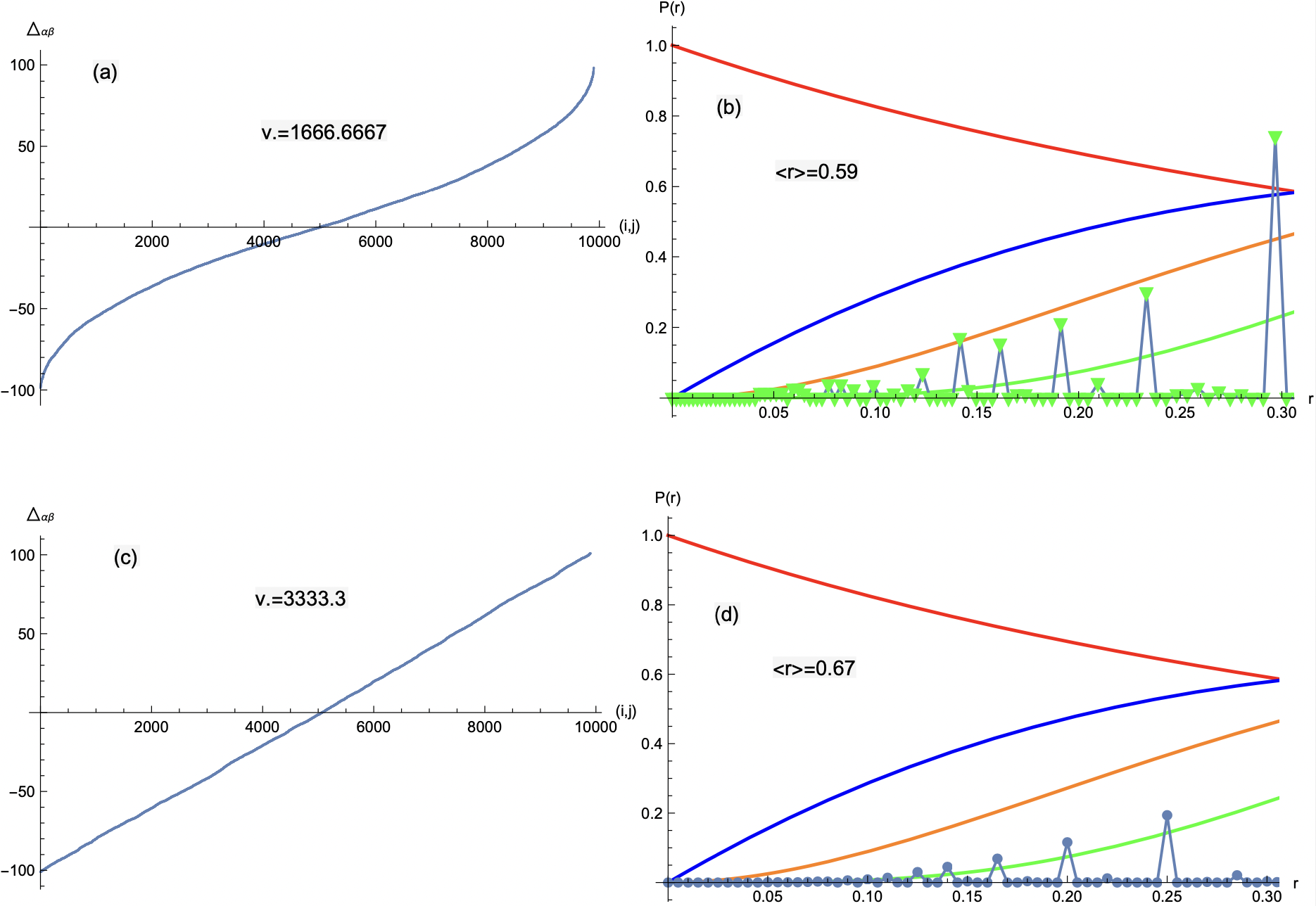
Figure 1: $\Delta_{\alpha\beta}$-spectrum for four-point interaction (a,b) which follows GUE distribution and two-point interaction (c,d) which follows GSE distribution. In this article we only show the results simulated by setting $N=100$.

where ${\bf Q}={\bf X}{\bf W^{Q}}$, ${\bf K}={\bf X}{\bf W^{K}}$, ${\bf V}={\bf X}{\bf W^{V}}$, are the query, key, and value matrices, which are all $N\times(N-1)$ type. ${\bf X}$ is the input $(\alpha,\beta)$ sequence. It is direct to know that when the potential difference DOF is unweighted (or selected) by the fermionic DOF, it behaves as a Gaussian variable, and the probabilities for $\Delta_{ij}=1,\cdots,(N-1)(i\neq j)$ are unequal, as shown in the simulaton-obtained spectrum in Fig.1(a,b), lower value of $\Delta_{ij}$ has bigger weight. In this case the net potential difference is zero and the variance is $\overline{\Delta_{ij}^{2}}\sim N^{2}/8$, and the level spacing distribution follows the GUE with $\langle r\rangle=0.59\sim 0.60$.

2.1 exact result

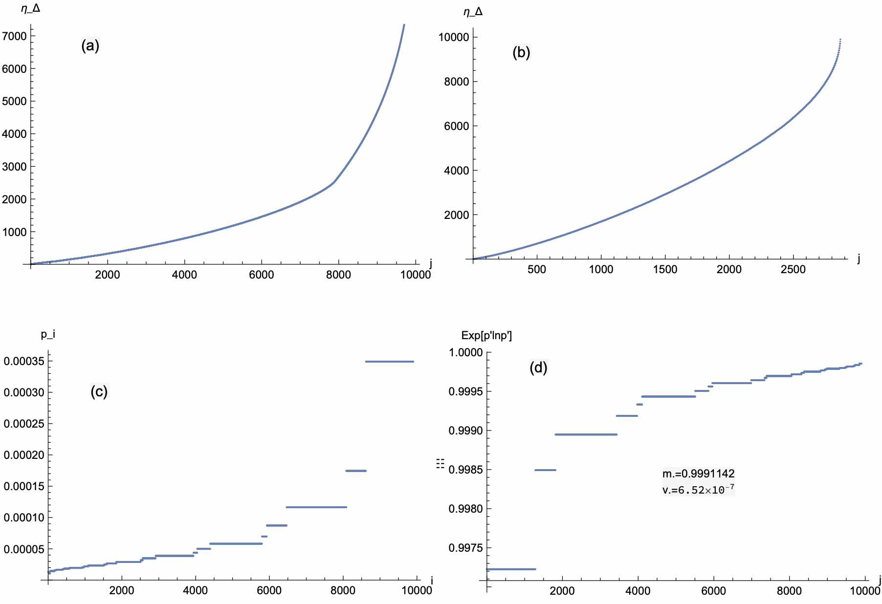
Figure 2: $\eta_{\Delta}$-spectrum for the unweighted $(\alpha,\beta)$-states (a) and the weighted one (b) which corresponds to inreducible group $\{\eta_{\Delta}\}$. For $N=100$, there will be nearly $O(M)\sim\frac{N^{2}}{4}$ flavors corresponding to distinct values of $\eta_{\Delta}$. (c) and (d) show the exact probabilities $p_{i}^{\eta}$ and $(p_{i}^{\eta})^{p_{i}^{\eta}}$ for each $(\alpha,\beta)$-state.

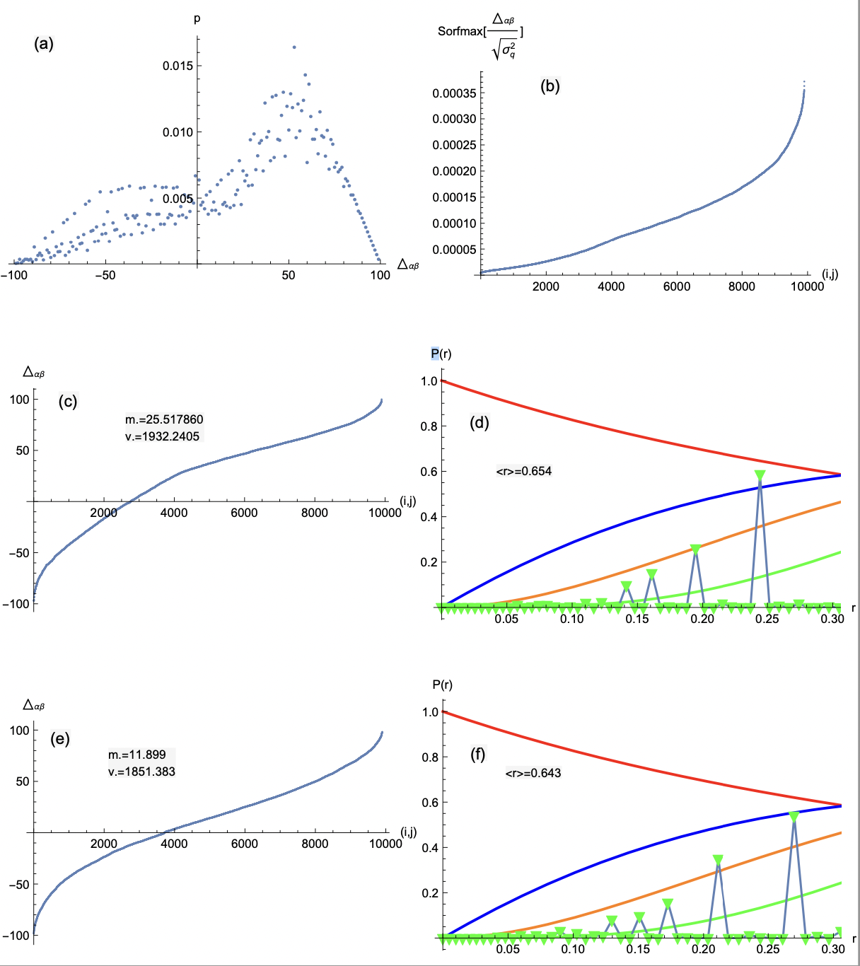
Figure 3: (a) Probability distribution of potential difference $\Delta_{\alpha\beta}$. (b) The softmax-renormalized results (the $QT^{T}$ matrix) which is available to inner product with the value matrix. (c,d) show the exactly calculated $\Delta_{\alpha\beta}$-spectrum and the level spacing distribution, while (e,f) show the predicted one using the learnable parameters in self-attention method.

To see the result when the $M$-DOF couples with the fermionic DOF, we firstly simulate the real case according to the calculated exact probabilities for each part of $(\alpha,\beta)$ according to the selection rule of fermions, $\partial_{{\alpha,\beta}}\eta_{\Delta}=0$, i.e., each value of $\eta_{\Delta}$ has the same weight in the final $\Delta_{\alpha,\beta}$-spectrum after the selection of fermionic $(i,j)$ parts. The calculated probabilities for each $(\alpha,\beta)$-state (i.e., the weight of each part of $(\alpha,\beta)$) arranged in order of value of $\eta_{\Delta}$ are shown in Fig.2(c). As we can see, now the probability distribution of potential difference changes and results in nonzero net value of potential differece. The resulting $\Delta_{\alpha,\beta}$-spectrum is shown in Fig.3(e,f), and the corresponding level spacing ratio follows a distribution between GUE and GSE.

3 predicted weight distribution using the algorithm

It is low efficiency to calculating one-by-one the probability of each part of $(\alpha,\beta)$ for large sample value $N$. Since there will be $\sim N^{2}/4$ distinct values of $\eta_{\Delta}$, which consist the group $\{\eta_{\Delta}\}$. By extracting the mean value and variance of $\eta_{\Delta}$ from the presence $\Delta_{\alpha\beta}$-spectrum, where we denote as ${\bf M}=[{\bf Q}{\bf K}^{T}]^{\eta_{\Delta}}$, and comparing to those quantities of the group $\{\eta_{\Delta}\}$ (where we denote as $m_{\eta}$ and $\sigma_{\eta}^{2}$, respectively), the actual probabilities (weights) for each $(\alpha,\beta)$-state can be predicted to high accuracy.

Macroscopically, there will be more repeating $\eta_{\Delta}$ in the low-value region as can be seem from the $\eta_{\Delta}$-spectrum, thus the mean value and variance of unbiased $\eta_{\Delta}$-spectrum will be always lower that the selected one ($\{\eta_{\Delta}\}$). Thus we, in first step, define the mean value $m_{0}$ as the maximal value of group $\eta_{\Delta}$, i.e., $m_{0}=N(N-1)$, and makeing the inner product ${\bf M}\cdot{\bf G}$, where $[{\bf Q}{\bf K}^{T}]_{\eta_{\Delta}}$ is the $N(N-1)$ extracted $\eta_{\Delta}$ arranging according to its value. Next,

$$G_{i\in[1,N(N-1)-|\delta_{i}|}={\rm exp}[\frac{-(\{M\}_{i}-m_{{\rm Max}[i]+\lambda_{i}})^{2}}{2\sigma_{M}^{2}}],$$ (3)

$$G_{i\in[(N(N-1)-|\delta_{i}|+1,N(N-1)]}=1,$$

where $|\delta_{i}|=0$ in the begining and the mean value $m_{{\rm Max}[i]+\lambda_{i}}$ is the ${\rm Max}[i]$-th element of the ascending-ordered $\{M\}_{i}$ group. We denote the index as $i=1,\cdots,N(N-1)$ representing the values of $\eta_{\Delta}$ in ascending order. $\sigma_{M}^{2}=\frac{1}{M^{\prime}}\sum_{i}^{M^{\prime}}(M_{i}-m_{0})^{2}$ is variance of elements in the group $\{M\}_{i}$ ($i=1,\cdots,M^{\prime}$) with $M^{\prime}\leq M$. $\delta_{i}\in[0,N(N-1))$ is learnable parameter (its variance step is defined according to the feed-back of mean value and variance of the weighted spectrum after the process of last time) which equals to zero in the begining, and it’s function here is to restricting the weighted-range to lower-$i$ regions, where has more number of repeating value of $\eta_{\Delta}$. While other elements of ${\bf G}$ are setted as 1. Here the mean value $m_{i}$ is defined according to the $(N(N-1)-\delta_{i})$-th value of ${\bf M}$, and $\lambda_{i}$ is a small quantity which is also a learnable parameter. Its sign ${\rm sgn}[\lambda_{i}]$ is negative when the ratio between mean value (variance) obtained from last iteration (we denote as the $l$-th learning) and that of the inreducible group $\{\eta_{\Delta}\}$ satifies $m_{l}/m_{\eta}\ll\sigma_{l}^{2}/\sigma_{\eta}^{2}$, and its sign should be positive in the opposite case that $m_{l}/m_{\eta}\gg\sigma_{l}^{2}/\sigma_{\eta}^{2}$. After each time of iteration (learning), the renewed spectrum be will obtained from the matrix ${\bf M}$ weighted by the rescaled $\prod_{j=1}^{l}G_{j}$ (by softmax process).

The iteration process of learning will stop when the $m_{l}$ and $\sigma_{l}^{2}$ are close enough to the standard values $m_{\eta}$ and $\sigma_{\eta}^{2}$, respectively. There are two ways to verify the final results, i.e., the obtained probabilities for each $(\alpha,\beta)$-state. First one is comparing the $\eta_{\Delta}$-spetrum and the level spacing distribution with the exactly calculated one, the second one is to measuring the distance between the predicted probabilities with the exactly calculated ones (denote as $p_{i}^{\eta}$). Instead of using the loss function $L=-\sum_{i}p_{i}^{\eta}{\rm ln}p_{i}$, we choose to calculate the mean value and variance of the group consist of the elements $p_{i}^{p_{i}^{\eta}}$, where both the predict and exact probabilities are arranged in ascending order of $\eta_{\Delta}$. While for the exact case, where all the predicted probabilities are the same with the real one, the mean value and variance of the group $\{(p_{i}^{\eta})^{p_{i}^{\eta}}\}$ are soly determined by the sample size $N$, where the mean value ($\sim 2(e^{1/M}-1)$) exponentially closes to zero and the standard deviation ($\sim 1-2(e^{1/M}-1)$) logarithmically closes to one with the increase of $N$.

4 numerical simulation results

According to the simulation, the variance of $\eta_{\Delta}$ spectrum $\sigma_{\eta}^{2}$ is lower but close to $\frac{N^{4}}{16}$ while that of the $\Delta_{\alpha\beta}$-spectrum is $\sigma_{\Delta}^{2}=\frac{N^{2}}{4}$ which is quite close to the flavor number of $\eta_{\Delta}$-DOF, i.e., $M\sim\frac{N^{2}}{4}$. Since the $\eta_{\Delta}$-DOF is a independent DOF relative to every $(i,j)$-part, this model is a three-DOF (or three-point all-to-all many-body system) system. As shown in Appendix.B, this can be illustrated in the fermion system by adding another scattering momentum-dependent DOF into the four-point fermion-fermion interacting system, and changes the variance of antisymmetry tensor from the four-point one ($\sim\frac{1}{4!}=\frac{g_{4}^{2}}{4N^{3}}$) to the three-point one ($\sim\frac{1}{3!}=\frac{g_{3}^{2}}{3N^{2}}$ where $g_{n}=\sqrt{\frac{n^{n-1}}{(n-1)!}}$ is a constant parameter with dimensions of energy).

The ratio between variance of $\Delta_{\alpha\beta}$-spectrum and $\eta_{\Delta}$ spectrum is close to $\frac{\sigma_{\Delta}^{2}}{\sigma_{\eta}^{2}}\sim\frac{4}{N^{2}}$. This is because for each fermion part, the probability for $M$ flavors of $\eta_{\Delta}$-DOF is $p_{\eta}=\frac{1}{M}\sim\frac{4}{N^{2}}$, while the unequivalent distribution of the probabilities (see Fig.3(a)) for each $\Delta_{\alpha\beta}$ (whose mean $\overline{p_{\Delta}}=\frac{1}{2N(N-1)}$) results in larger uncertainty, and this uncertainty results in stronger thermalization effect (compares to the original one) and smaller variance for the $\Delta_{\alpha\beta}$-spectrum which is $\leq\frac{N^{2}}{4})$. In this case the potential difference is a Chi-square variable and has nonzero expectation value. This part of nonzero potential difference corresponds to the UV cutoff in position space as well as the long-wavelength limit for the scattering momenta, which is a signature for the polarons following the Wigner-Dyson distribution. And the resulting distribution is of an intermediate region between GUE and GSE. While in original $\Delta_{\alpha\beta}$-spectrum as shown in Fig.1(a,b), the potential difference is a Gaussian variable with zero mean (and thus zero expectation value for the polaronic effect) and the many-body behavior follows the GUE distribution. Also, this case belongs to the four-point-type fermion interaction, with variance $\sigma_{4-p}^{2}\sim\frac{4N^{2}}{4!}=\frac{N^{2}}{6}$, and its level spacing follows GUE distribution ($\langle r\rangle\sim 0.59$). While the two-point-type fermion interaction (with much stronger thermalization), as shown in Fig.1(c,d), it has a variance which is twice of the four-point one, $\sigma^{2}_{2-p}=\frac{N^{2}}{2!}\frac{2}{3}=\frac{N^{2}}{3}$, and its level spacing follows GSE distribution ($\langle r\rangle\sim 0.67$). Then it is reasonable for the intermediate case we studied here, whoes variance $\sigma_{\Delta}^{2}\sim\frac{N^{2}}{4}$ is between the two-point one and four-point one, and follows the ensemble between GUE and GSE with $\langle r\rangle=0.63\sim 0.65$. More critically, the variance $\sigma_{\Delta}^{2}$ is in fact $N$-dependent even for $N\rightarrow\infty$. If we treating it as an inner product by four-point variance and two-point variance weighted by different probabilities, an experimental expression could be

$$\sigma_{\Delta}^{2}=(1-\frac{1}{{\rm ln}N^{2}}[\sigma^{2}_{2-p},\sigma_{4-p}^{2}]\cdot{\rm Softmax}[1,2]\approx(1-\frac{1}{{\rm ln}N^{2}}(0.2689\sigma^{2}_{2-p}+0.731\sigma_{4-p}^{2}).$$ (4)

For example, for $N=100,150,200$, the corresponding variances $\{\sigma_{2-p}^{2},\sigma_{\Delta}^{2},\sigma^{2}_{4-p}\}$ are $\{3333.3,\ 1954,\ 1666.5\}$, $\{7500,\ 4355,\ 3750\}$, and $\{13421,\ 7674.1,\ 6666,6\}$, respectively. There is a trendency which is persistent for artitaryly large-$N$: the variance of such intermediate state depends on both the other two variances, $\sigma_{2-p}^{2}$ and $\sigma_{4-p}^{2}$ whose values can be soly determined in large-$N$ limit, and with $N$ increasing, the $\sigma_{\Delta}^{2}$ will more and more close to the four-point one $\sigma_{4-p}^{2}$ (compares to $\sigma_{2-p}^{2}$) with a decreasing but never vanished velocity. This indeed reflects a spontaneous localization, and the suppressed thermalization with the increasing $N$.

5 algorithm

5.1 method

Here we show the principle for this algorithm to predicting the sample weight distribution through the mean value and variance estimated in few-position. During the steps of automatic iterations, the criterion is to matching the mean value and variance of the predicted spectrum with the reduced one (inreducible group, which has much small sample size). This base on the rule that for every weighted group that containing only two elements, its variance will never be changed when we modify there corresponding weights, even if the summation of there corresponding weights not equals to one, by the mean value will changes in this process.

For example, for a group ${k_{1},k_{2}}$ weighted by ${w_{1},w_{2}}$, the variance reads (we use the bias-corrected sample variance here)

$$\sigma^{2}=\frac{\sum_{i}w_{i}(k_{i}-m_{k})^{2}}{\sum_{i}w_{i}-\frac{\sum_{i}w_{i}^{2}}{\sum_{i}w_{i}}},$$ (5)

where $m_{k}=\sum_{i}k_{i}w_{i}/\sum_{i}w_{i}$ is the weighted mean value. This expression is equivalents to replacing $w_{2}$ by $(1-w_{1})$ and omit the $\sum_{i}w_{i}$ in the denominator, i.e., $\sigma^{2}=\frac{\sum_{i}w_{i}(k_{i}-m_{k})^{2}}{1-\sum_{i}w_{i}^{2}}$. Thus next we consider only the case $\sum_{i}w_{i}=1$. Then we introduce another one with modified weight distribution $\{w^{\prime}_{1},w^{\prime}_{2}\}:=\{w_{1}+w_{d},w_{2}-w_{d}\}$. These two groups have the same variance

$$\sigma^{2}=\frac{1}{2}(k_{1}-k_{2})^{2}=\frac{(k_{1}-k_{2})^{2}\prod_{i}w_{i}}{1-\sum_{i}w_{i}^{2}}=\frac{(k_{1}-k_{2})^{2}(\prod_{i}w_{i}-w_{d}^{2}+w_{d}(1-2w_{1}))}{1-\sum_{i}w^{\prime}_{i}{}^{2}}.$$ (6)

This can be explained using the method we discussed in Ref.[1], i.e., expressing thic common variance $\sigma^{2}$ in terms of a limiting result of the infinitely scaled variable $\chi$ (the detailed form of this variable does not have to known), which has the form $\sigma^{2}:=\lim_{\chi\rightarrow\infty}f=\frac{f}{1-\partial_{\chi}f}$. In above expression the summation of squared weights of these two groups can be treated as there corresponding derivative terms with respect to $\chi$,

$$\sum_{i}w_{i}^{2}=1-2w_{1}(1-w_{1}),\sum_{i}w^{\prime}_{i}{}^{2}=2(-w_{d}^{2}+(1-w_{1})w_{1}+w_{d}(1-2w_{1})).$$ (7)

For first group, by defining $\prod_{i}w_{i}=w_{1}(1-w_{1}):=f_{\chi}$, we have

$$\frac{1}{2}=\lim_{\chi\rightarrow\infty}f_{\chi}=\frac{f_{\chi}}{1-\partial_{\chi}f_{\chi}},$$ (8)

$$1-2f_{\chi}=\partial_{\chi}f_{\chi},$$

$$\frac{1}{2}(k_{1}-k_{2})^{2}=\lim_{\chi\rightarrow\infty}(k_{1}-k_{2})^{2}f_{\chi},$$

$$1-2f_{\chi}=\partial_{\chi}[(k_{1}-k_{2})^{2}f_{\chi}].$$

There are two possible cases which correspond to different representations. The first one is the representation in unit of $(k_{1}-k_{2})^{2}$ which is independent with $\chi$. This case will leads to $w_{i}=\frac{1}{2}\pm\frac{i}{2}$. The second one is the representation in unit of $\lim_{\chi\rightarrow\infty}f_{\chi}=\frac{1}{2}$. In this representation, the acceptable results, $w_{i}=\frac{1}{2}$ can be solved. Note that for this case, the derivative term $\partial_{\chi}f_{\chi}$ in the second line of above expression indeed corresponds to $\partial_{\chi}w_{1}=(1-w_{1})$ and $\partial_{\chi}w_{2}=\partial_{\chi}(1-w_{1})=w_{1}$, which mean the variable $\chi$ is scalable by $1$ (which is no more a constant here), and $\partial_{\chi}1=1$. Here $1=e^{i(2\pi-0^{+})}$, where $0^{+}$ denotes an infinitely small shiftment in phase and generate the imaginary part into the previous representation, and the cutoff of this infinitely small imaginary part (which is the UV cutoff in momentum space if we projecting this imaginary part into the position space) determines directly the largest quantity that could be independent with $\chi$, i.e., the unit quantity in this representation ($1/2$). Thus more rigorously we have $\partial_{\chi}f_{\chi}=1^{2}-2f_{\chi}$ with $1^{2}\neq 1$ and $\partial_{\chi}1\neq\partial_{\chi}1^{2}$. Here this cutoff is necessary to fix the tolerance of whole system, i.e., $\partial_{\chi}\frac{1}{2}=|\frac{1}{2}-\frac{1}{2+\frac{1-1^{2}}{f_{\chi}}}|=0$. Substituting the second line of above expressions into the expanded expression in the last line, we have

$$\partial_{\chi}(k_{1}-k_{2})^{2}=\frac{1-2f_{\chi}}{f_{\chi}}[1-(k_{1}-k_{2})^{2}]=\frac{\partial_{k}f_{\chi}}{f_{\chi}}[1-(k_{1}-k_{2})^{2}].$$ (9)

In the mean time, due to the invariant property of the infinite scale, $\partial_{\chi}\lim_{\chi\rightarrow\infty}f_{\chi}=0$, the first line of Eq.(LABEL:o0) results in the relation

$$\frac{1-2f_{\chi}}{2f_{\chi}}=-f_{\chi}\partial_{\chi}\frac{1}{2f_{\chi}}.$$ (10)

Substituting this into Eq.(9), we can obtain

$$\frac{1-(k_{1}-k_{2})^{2}}{\partial_{\chi}(k_{1}-k_{2})^{2}}=\frac{1}{2}\frac{-1}{f_{\chi}\partial_{\chi}\frac{1}{2f_{\chi}}}=\frac{f_{\chi}}{\partial_{\chi}f_{\chi}}.$$ (11)

Thus we can make sure that there must be another $\prod_{i}w_{i}$-related variable $\chi^{\prime}$ satisfying

$$\lim_{\chi^{\prime}\rightarrow\infty}f_{\chi^{\prime}}=\frac{\partial f_{\chi}}{\partial(k_{1}-k_{2})^{2}},$$ (12)

$$\partial_{\chi^{\prime}}f_{\chi^{\prime}}=(k_{1}-k_{2})^{2}.$$

Using the property $\frac{f_{\chi}}{\partial_{\chi}f_{\chi}}\equiv\lim_{\chi\rightarrow\infty}f_{\chi}\frac{f_{\chi}}{\lim_{\chi\rightarrow\infty}f_{\chi}-f_{\chi}}$, we have

$$f_{\chi}=\frac{-\partial_{\chi}f_{\chi}}{1-\partial_{\chi}f_{\chi}}\frac{1}{\partial_{\chi}\frac{1}{2f_{\chi}}},$$ (13)

$$=\frac{\partial f_{\chi}}{\partial(k_{1}-k_{2})^{2}}[1-(k_{1}-k_{2})^{2}].$$

Combined with Eq.(9), we obtain the following form of the limiting scale

$$\lim_{\chi\rightarrow\infty}f_{\chi}=\frac{1}{2}=f_{\chi}-f_{\chi}^{2}\partial_{\chi}\frac{1}{2f_{\chi}}.$$ (14)

Besides, using Eq.(11) and the derivative of the ratio between two limits $\frac{\lim_{\chi\rightarrow\infty}[(k_{1}-k_{2})^{2}f_{\chi}]}{\lim_{\chi\rightarrow\infty}f_{\chi}}=(k_{1}-k_{2})^{2}$, we obtain

$$\partial_{\chi}{\rm ln}\frac{1}{\lim_{\chi\rightarrow\infty}f_{\chi}}=\partial_{\chi}{\rm ln}2$$ (15)

$$=\frac{\partial_{\chi}f_{\chi}}{f_{\chi}}\frac{1-(k_{1}-k_{2})^{2}}{(k_{1}-k_{2})^{2}}$$

$$=\frac{\partial_{\chi}(k_{1}-k_{2})^{2}}{(k_{1}-k_{2})^{2}}.$$

Thus we have, $\frac{\partial_{\chi}2}{2}=\frac{\partial_{\chi}(k_{1}-k_{2})^{2}}{(k_{1}-k_{2})^{2}}$, thus in the limit of $\partial_{\chi}2\rightarrow 2$, $(k_{1}-k_{2})^{2}\rightarrow e^{i(2\pi-0^{+})}=e^{\chi}$ and $\frac{\partial_{\chi}(k_{1}-k_{2})^{2}}{(k_{1}-k_{2})^{2}-1}\rightarrow\frac{\partial_{\chi}(k_{1}-k_{2})^{2}}{(k_{1}-k_{2})^{2}}$. To looking for real solution, in this limit we have $(k_{1}-k_{2})^{2}=e^{\chi}\sim 1$, i.e., $\lim_{\chi\rightarrow\infty}|k_{1}-k_{2}|\gg|k_{1}-k_{2}|$. This fact reveals the reason why the variance of such binary group will always keep invariant when we modify the weight distribution or change the value of elements, as long as the distance between two elements is invariant. This is consistent with the fact that $|k_{1}-k_{2}|\propto\delta\chi$ as they all describe the distance in the position space, while the corresponding long wavelength limit in momentum space after fourier transformation can be realized by the factor $[1-(k_{1}-k_{2})^{2}]^{-1}$. Also, the unit quantity expressed in terms of the limiting relation as shown in eq.(14) allows the easier derivation along the distances in the position space. For example, if we consider beyond the binary groups by replacing $f_{\chi}=w_{1}(1-w_{i})$ as the variance for the binary group in its position, then the $[\partial_{\chi}\frac{1}{2f_{\chi}}]^{-1}$-term in Eq.(14) can indeed be regarded as the variance of another group (with more elements) in position next to the former one. To illustarting this, we set the binary group in the first position as $(k_{1},k_{N})$ whose variance denoted as $v_{1}$, and the one in the next position as $(k_{1},k_{1}+1,k_{N}-1,k_{N})$ whose variance denoted as $v_{2}$. The other groups with more elements are arranged in the same manner. Then the slope in the position space is equivalents to the variance ratio $\frac{v_{1}-v_{2}}{v_{2}-\frac{v_{2}^{2}}{v_{1}}}=\frac{v_{1}}{v_{2}}$, where $(v_{2}-\frac{v_{2}^{2}}{v_{1}})$ is the smallest step length here appearing in the same form with Eq.(14), i.e., the IR cutoff in the position space. Such unit length as well as the slope are not invariant between arbitaryly two positions with different numbers of element, and this length reduces to zero efficiently for higher-order position derivative. For example, by setting $k_{N}=13$, the first to fourth-order derivative are $-6.4918,\ 0.84579,\ 0.040513,\ 0.0093128$, respectively, and the highest-order one (the twelfth-order derivative) is $0.000030169$.

It can be checked that, in this representation, where both the elements and weights are dependent with $\chi$, the real solution of weights $w_{i}=\frac{1}{2}=\partial_{\chi}f_{\chi}=(k_{1}-k_{2})^{2}[1-\frac{1}{2\lim_{\chi\rightarrow\infty}(k_{1}-k_{2})^{2}}](f_{\chi}=\frac{1}{4})$ can be obtained, where $\partial_{\chi}\frac{1}{2f_{\chi}}=-4$. In the mean time the infinite $\chi$ corresponds to the simultaneous scalings of $w_{i}\rightarrow\frac{1}{2}$ and $w_{d}^{2}\rightarrow 0$ for the second group, which results in the same result of variance. Thus for such kind of binary groups, we can soly modify the mean value and keep the variance be invariant. To modify the variance, the simplest way is by introducing the third element, which can be viewed as a collection of all the other elements in the reducible group $\{\alpha,\beta\}$ other that the two elements in both sides of the position that the algorithm kernel working on. Once a position is initially determined, the elements in two sides of this position will be treated as a part of binary (summation of weights is one), then the mean value can be increased by giving more weight to the right-side one, which corresponds to larger value of $\eta_{\Delta}$. Then other elements enter this group play the role of third element to available the adjustment for the variance. In Eq.(LABEL:xo), the learnable mean value $m_{i+\lambda_{i}}$ at position $i=i^{\prime}$ can be adjusted with the range of $[\{M\}_{i^{\prime}},\{M\}_{N(N-1)}]$. As the subscript of this learnable mean parameter decreasing from the largest one $N(N-1)$ (corresponds to the position at the end of spectrum), the resulting mean value and variance of the updated $\eta_{\Delta}$-spectrum will both be increased at first and then keep decreasing until the subscript decreases to $i=i^{\prime}$. During this process, there will be a certain position will the mean value is enhanced while the variance is reduced (compares to the former spectrum before the update of parameters).

In this way, the learnable-parameter-dependent step lengths control the positions where the algorithm modifies the weight distribution step-by-step, and the ratio between mean value and variance can be modified until the spectrum exhibits features match enough to the one corresponding to the inreducible group.

5.2 criterion

Except the above-introduced method to estimate the fitness between the predicted mean value and variance with the exact ones, there is another criterion using the $\beta_{en}$-factor ($\beta_{en}=1,2,4$ for GOE, GUE, and GSE ensembles). As the joint probability density function for Gaussian ensembles[39] satisfies

$$P_{joint}=C_{\beta,N}\prod_{i<j}|k_{i}-k_{j}|^{\beta_{en}}e^{-\frac{1}{2}\sum_{i}^{N}(k_{i}-m_{k})},$$ (16)

where the normalization parameter reads

$$C_{\beta,N}=\frac{1}{(2\pi)^{N/2}}\prod_{j}^{N}\frac{\Gamma[1+\frac{\beta_{en}}{2}]}{\Gamma[1+j\frac{\beta_{en}}{2}]}.$$ (17)

Then accroding to the above-introduced algorithm, we start with an ascending-ordered original $\eta_{\Delta}$-group (unreducible) $\{M\}_{i=1,\cdots,N(N-1)}:=\{k_{1},\cdots,k_{N(N-1)}\}$ following GUE distribution (whose mean value and variance are denoted as $m_{o}$ and $\sigma^{2}_{o}$, respectively), in first round of learning, we obtain the weight distribution for all elements by lifting the mean value to the largest one ($k_{max}$), then this results in a new variance

$$\sigma_{M}^{2} =\frac{\sum^{N(N-1)}_{i}(k_{i}-k_{max})^{2}}{N(N-1)[1-\frac{1}{N(N-1)}]}=\frac{\sum^{N(N-1)}_{i}(|k_{max}-m_{o}|+|k_{i}-m_{o}|\theta(k_{o}-k_{i})-|k_{i}-m_{o}|\theta(k_{i}-k_{o}))^{2}}{N(N-1)[1-\frac{1}{N(N-1)}]}$$ (18)

$$=\frac{\sigma_{o}^{2}(N(N-1)-1)+N(N-1)|m_{o}-k_{max}|^{2}}{N(N-1)-1},$$

where the factor $|m_{o}-k_{max}|^{2}$ can be much easily obtained from the summation of all elements as well as the two mean values

$$|m_{o}-k_{max}|^{2}=N(N-1)[(k_{max}^{2}-m_{o}^{2})+2(m_{o}-k_{max})\sum_{i}k_{i}],$$ (19)

Also, the summation of squared elements can be obtained $\sum_{i}k_{i}^{2}=\sigma_{o}^{2}(N(N-1)-1)-N(N-1)m_{o}^{2}+2m_{o}\sum_{i}k_{i}$, and then we can know that all the antisymmetry-allowed combinations ($i<j$) in the second term of above joint probability density function have an available summation

$$\sum_{i<j}|k_{i}-k_{j}|^{2}=\sum_{i}k_{i}^{2}(N(N-1)-1)-[(\sum_{i}k_{i})^{2}-\sum_{i}k_{i}^{2}].$$ (20)

Then in this algorithm, we letting each element (eigenvalues) in the group $\{M\}_{i}$ weighted by the factors ${\rm softmax}\{e^{-(k_{i}-k_{max})^{2}/(2\sigma_{M}^{2})}\}_{i}$ (using the variance $\sigma_{M}^{2}$ defined-above), then if we substituting the resulting variance of these weigthed eigenvalues back to the joint eigenvalue probability density function of the original one in GOE ensemble (with the normalization constant $C_{2,N}$), we can obtain an increased factor of $\beta_{en}$ (between 2 and 4) for the Lebesgue measure[38], i.e., the second term of $P_{joint}$. Next we rewrite the maximal index in the group $\{M\}_{i}$ as $N(N-1)\equiv n$ for simplicity in notation.

We know the antisymmetry product $\prod_{i<j}|k_{i}-k_{j}|^{\beta_{en}}$ equivalents to the van der Monde determinant,

$$\prod_{i<j}|k_{i}-k_{j}|^{\beta_{en}}=({\rm Det}\begin{pmatrix}1&k_{1}&k_{1}&\cdots&k_{1}\\ 1&k_{2}&k_{2}^{2}&\cdots&k_{1}^{n-1}\\ \cdots&&&&\\ 1&k_{n}&k_{n}^{2}&\cdots&k_{N}^{n-1}\\ \end{pmatrix})^{\beta_{en}}.$$ (21)

To clarify the effect of the variant $\beta_{en}$ on this term, we using the tridiagonal matrix lemmas[39]. Assuming the above van der Monde matrix can be transformed into a tridiagonal symmetry matrix with diagonal element $T_{d}$ and subdiagonal elements $T_{i}(i=1,\cdots,N-1)$ arranged in the form

$$T_{n}=\begin{pmatrix}t_{d}&t_{n-1}&0&\cdots&0&0\\ t_{n-1}&T_{d}&t_{n-2}&\cdots&0&0\\ 0&t_{n-2}&T_{d}&\cdots&0&0\\ \cdots&&&&&\\ 0&0&0&\cdots&t_{1}&t_{d}\\ \end{pmatrix}.$$ (22)

For this matrix, we have ${\rm Det}T_{n}=t_{d}{\rm Det}T_{n-1}-t^{2}_{n-1}{\rm Det}T_{n-2}$, where $t_{n-1}$ is the $(n-1)\times(n-1)$ lower right-corner submatrix of $T_{N}$ and $k_{j}^{(n-1)}$ are its eigenvalues. There is another relation[39] $\prod_{i}(k_{j}^{(m)}-k_{i}^{(n)})=(k_{j}^{(m)}-t_{d})\prod_{i}(k_{j}^{(m)}-k_{i}^{(n-1)})-t_{n-1}^{2}\prod_{i}(k_{j}^{(m)}-k_{i}^{(n-2)})$, where $m\in[2,n]$ with corresponding $j\in[1,m]$. For $m=n$, both sides of this equation are zero.

For ascending ordered eigenvalues of $T_{M}$ ($M=n,n-1,\cdots,2$), the total number of eigenvalues for these (sub)matrices satisfy $\sum_{i=1}^{M+1}k_{i}^{(M+1)}-\sum_{j=1}^{M}k_{j}^{(M)}=t_{d}$, i.e., the summation of all eigenvalues for two adjacent (sub)matrices always differed by the diagonal element $t_{d}$, Also, $\prod_{i=1}^{(n)}(k_{i}^{n}-k_{1}^{(M^{\prime})})=\prod_{i=1}^{n}(k_{i}^{(n)}-k_{M^{\prime}}^{(M^{\prime})})$ where $M^{\prime}=N-1,\cdots,2$, and $k_{1}(k_{M^{\prime}})$ corresponds to the smallest (largest) eigenvalue of the submatrix $T_{M^{\prime}}$. We also know that $\prod_{i,j}(k_{i}^{(N)}-k_{j}^{(N-1)})=\prod_{i}^{n-1}t_{i}^{2i}$, and $\prod_{i,j}(k_{i}^{(n)}-k_{j}^{(n-2)})=t_{1}^{2}\prod_{i}^{n-1}t_{i}^{2i}$.

The product of the eigenvalue permutations of $T_{N}$ in ensemble $\beta_{en}$ satisfies the following relation according to the algebraic fact

$$\prod_{i<j}|k_{i}-k_{j}|^{2\beta_{en}}=\frac{\prod_{i=1}^{n-1}t_{i}^{2i}}{\prod_{i=1}^{n}Q_{i}^{2\beta_{en}}}=\frac{\prod_{1\leq i\leq n,1\leq j\leq n-1}(k^{(n)}_{i}-k_{j}^{(n-1)})}{\prod_{i}^{n}Q_{i}^{2\beta_{en}}},$$ (23)

where $\prod_{i}Q_{i}$ is the product of elements in the first row of eigenvector matrix of $T_{n}$.

According to the above discussion and simulations, we know that the self-modified parameters lifting the variance of eigenvalues by changing the weight distribution and thus lifting the ensemble index in normalized Lebesgue measure (i.e., the product of the eigenvalue permutations) of the joint eigenvalue probability density function. The ensemble index $\beta_{en}$ will finally be increased from 2 to a larger one $\beta^{\prime}_{en}$ which is between 2 and 4 and reveals a distribution between GUE and GSE. During this process, the changes of product term $\prod_{i<j}|k_{i}-k_{j}|^{2\beta_{en}}$ can be visualized by the product of the eigenvectors $\prod_{i=1}^{n}Q_{i}^{2\beta_{en}}$. When the change $\beta_{en}\rightarrow\beta_{en}^{\prime}$ happen, the variance of $\prod_{i=1}^{n}Q_{i}^{2\beta_{en}}$ reads

$$\prod_{i}Q_{i}^{2\beta}(\prod_{i}Q_{i}^{2(\beta^{\prime}_{en}-\beta_{en})}-1)=\frac{\prod_{i}t_{i}^{2i\beta_{en}}(\prod_{i}t_{i}^{2i(\beta^{\prime}_{en}-\beta_{en})}-\prod_{i<j}|k_{i}-k_{j}|^{2(\beta^{\prime}_{en}-\beta_{en})})}{\prod_{i<j}|k_{i}-k_{j}|^{2\beta^{\prime}_{en}}}.$$ (24)

Then if we rescale the change $\beta_{en}\rightarrow\beta_{en}^{\prime}$ to another one: $\beta^{\prime}_{en}\rightarrow\infty$, which can be realized by another two scalings that happen simultaneously: $\beta_{en}\rightarrow\infty-|\beta_{en}-\beta_{en}^{\prime}|$ and $\prod_{i}Q_{i}^{2}\rightarrow 0$ (and thus $\beta_{en}$ and $\beta_{en}^{\prime}$ are still independent with each other). From above equation, we can define the following function of $\beta^{\prime}_{en}$

$$f_{\beta^{\prime}_{en}}:=\frac{\prod_{i<j}|k_{i}^{(n)}-k^{(n)}_{j}|^{2(\beta^{\prime}_{en}-\beta_{en})})-\prod_{i}t_{i}^{2i\beta_{en}}(\prod_{i}t_{i}^{2i(\beta^{\prime}_{en}-\beta_{en})}}{\prod_{i<j}(k_{i}^{(n)}-k_{j}^{(n)})^{2\beta^{\prime}_{en}}}.$$ (25)

Then we have

$$\frac{f_{\beta^{\prime}_{en}}}{\lim_{\beta^{\prime}_{en}\rightarrow\infty}f_{\beta^{\prime}_{en}}}=1-\partial_{\beta^{\prime}_{en}}f_{\beta^{\prime}_{en}},$$ (26)

where

$$\lim_{\beta^{\prime}_{en}\rightarrow\infty}f_{\beta^{\prime}_{en}}=\prod_{i<j}(k_{i}^{(n)}-k_{j}^{(n)})^{-2\beta_{en}},$$ (27)

$$\partial_{\beta^{\prime}_{en}}f_{\beta^{\prime}_{en}}=\prod_{i}Q_{i}^{2\beta^{\prime}_{en}}\frac{{\rm ln}\prod_{i}Q_{i}^{2}}{\prod_{i}t_{i}^{2i\beta}}.$$

Since the above rescaling actions endow the $\beta_{en}$-dependence (instead of $\beta_{en}^{\prime}$) to the term $\prod_{i}Q_{i}^{2\beta^{\prime}_{en}}$, i.e., $-{\rm ln}\prod_{i}Q_{i}^{2\beta^{\prime}_{en}}\equiv\prod_{i<j}(k_{i}^{(n)}-k_{j}^{(n)})^{2\beta_{en}}$, which scales to infinity acompnied by $\beta^{\prime}_{en}\rightarrow\infty$, and this equility will not be broken even before the limit $\beta^{\prime}_{en}\rightarrow\infty$ is arrived, i.e., it is valid even when the $\beta_{en}^{\prime}$-dependence of $f_{\beta_{en}^{\prime}}$ not yet fade away.

Similar to the conformal field theories, the decrease of effective number of DOF under renormalization group is important to gain further understanding for the complex systems. Here we add more detailed explainations about the scaling behaviors in above subsection. Firstly we replacing the normal ensemble change $\beta_{en}=2\rightarrow\beta_{en}^{\prime}\in(2,4)$ by another ones: $\beta_{en}^{\prime}\rightarrow\infty$; $\prod_{i}Q_{i}^{2}\rightarrow 0,\prod_{i<j}(k_{i}^{(n)}-k_{j}^{(n)})^{2\beta_{en}}\rightarrow\infty$. Under this, the independence between $\beta_{en}(Q_{i})$ with $\beta_{en}^{\prime}$ are preserved just like the original case. But in the mean time, we have to endow the $Q_{i}$-related product term with the $\beta_{en}$-dependence, in other world, this combine the $Q_{i}$ and $\beta_{en}$ DOFs. To make sure alll these requirements are meeted, as the $\beta_{en}^{\prime}$ scales to infinity, $\beta_{en}$ has to scale to $(\infty-(\beta^{\prime}_{en}-\beta_{en}))$. There is an essential logical relation between $\beta_{en}$ and $\beta_{en}^{\prime}$. As $\beta_{en}^{\prime}$ scales to infinity at first, $\beta_{en}^{\prime}+\infty\rightarrow\infty$, the locked $\beta_{en}$ scales as $\beta_{en}\rightarrow\beta_{en}+\infty-(\beta_{en^{\prime}}-\beta_{en})$. That means in any moment, the detail value of $\beta_{en}$ cannot be obtained before $(\beta^{\prime}_{en}-\beta_{en})$, i.e., the derivative of $\beta_{en}$ with $\beta^{\prime}_{en}$, is known. Thus we have

$$\frac{\partial\beta_{en}}{\partial\beta_{en}^{\prime}}=\frac{\infty-(\beta_{en}^{\prime}-\beta_{en})}{\infty},$$ (28)

where the numerator is the variance of $\beta_{en}$ which can found to be depends on itself only. We have

$$\beta_{en}=\infty-(\beta_{en}^{\prime}-\beta_{en})=\frac{\infty-(\beta_{en}^{\prime}-\beta_{en})}{\frac{\infty}{\beta_{en}^{\prime}-\beta_{en}}}\frac{\partial(\beta_{en}^{\prime}-\beta_{en})}{\partial(1-I_{0})},$$ (29)

where $I_{0}=(\beta_{en}^{\prime}-\beta_{en})-\frac{(\beta_{en}^{\prime}-\beta_{en})^{2}}{\beta_{en}^{\prime}}$ is the unit step in this derivative and this derivative can be obtain using the method we introduced in Sec.4.2,

$$\frac{\partial(\beta_{en}^{\prime}-\beta_{en})}{\partial(1-I_{0})}=\frac{\infty-(\beta_{en}^{\prime}-\beta_{en})}{I_{0}}=\frac{\infty}{\beta_{en}^{\prime}-\beta_{en}}.$$ (30)

Thus that means the $I_{0}$ and $1$ in the denominator of first line are in fact not in the same domain, and once they appear together through the algebra-allowed limiting-scale-assistanted domain transition, we can in fact write $I_{0}$ more strictly as $1^{-}:=e^{i(2\pi-0^{-})}$, and similar to the derivative of $\frac{\partial\beta_{en}}{\partial\beta_{en}^{\prime}}$, their relations can be understood by $1\mapsto\beta_{en}^{\prime}+\infty$, $I_{0}\mapsto\infty$. We can resubstituting this $\beta_{en}$ back to the above expression of $\frac{\partial\beta_{en}}{\partial\beta_{en}^{\prime}}$ repeatly,

$$\frac{\partial(\beta_{en}^{\prime}-\beta_{en})}{\partial(1-I_{0})}=\frac{\partial-\frac{\partial(\beta_{en}^{\prime}-\beta_{en})}{\partial(1-I_{0})})}{\partial(1-I_{0})}=\cdots,$$ (31)

and we can obtain the vanishing variance of $\beta_{en}$ at a certain order $N$ as $\frac{\partial^{(N)}(\beta_{en}^{\prime}-\beta_{en})}{\partial(1-I_{0})^{N}}=0$, and whatever which IR cutoff we set (through this order $N$), the variance of $\beta_{en}$ will vanishes faster than the one in its next hierarchy $\beta_{en}^{\prime}$.

Similarly, the derivative of the function $f_{\beta_{en}^{\prime}}$ can be rewritten as

$$\frac{\partial f_{\beta_{en}^{\prime}}}{\partial\beta_{en}^{\prime}}=\frac{\prod_{i}Q_{i}^{2\beta_{en}}}{\partial(1-I_{0}^{\prime})},$$ (32)

where

$$I_{0}^{\prime}=\prod_{i}Q_{i}^{2\beta_{en}}-\frac{\prod_{i}Q_{i}^{4\beta_{en}}}{\prod_{i}Q_{i}^{2\beta^{\prime}_{en}}},$$ (33)

and we also have

$$\prod_{i}Q_{i}^{2\beta^{\prime}_{en}}=2(I+\prod_{i}Q_{i}^{2\beta_{en}})-1.$$ (34)

6 Conclusion

We reveal the relation between UV cutoff of polaronic momentum $\Lambda_{q}$ and its SYK behavior. The SYK behavior of a polaron system, as well as the relation between scattering momentum and the related statistical behaviors has rarely been investigated before. By projecting to a 2d square lattice, The algorithm designed by us allow the automatically optimization and prediction for the resulting spectrum. In this 2d lattice model with position space representation, the emergent nonzero expectation value of site potential difference $\Delta_{\alpha\beta}$ shows the existence of polaron. For eigenvalues arranged in ascending order in the position space, the learning program devotes to predict the weight distribution of each eigenvalue in the final spectrum, which is realized by modifying the relative distance between each pair of the two elements (groups) in both sides of the selected positions. Indeed this is equivalents to modifying the step length for each position, i.e., the IR cutoff in the position space, but this cutoff is nolonger a invariant constant here. One of the obvious advance of this is the much easier estimation of the derivative of potential difference in each position, which is directly related to the variance as well as mean value of the final spectrum. Also, the large distance in the lattice position space (like the scaled variable $\chi$) corresponds to the long wavelength limit in the momentum space.

In momentum space, as the polaron emerges at the pole of scattering amplitude, the polaronic momentum $q$, which is also the relative momentum during scattering between impurity and majority particles (or holes), reads $q=ia^{-1}$. The quantity $qa$ is also an important characteristic scale in predicting its many-body behaviors. As we show in the Appendix, the polaron system in momentum space with four-fermion interactions, the modified level distribution (from GUE to another one between GUE and GSE) can be described and explained in terms of the additional momentum $q$-dependent Guassian wave functions $\Phi_{ik}$ and $\Phi_{jl}$.

7 Appenidx.A: Emergent polaron in terms of momentum space representation

Similar to Eq.(1), we can illustrating this model in momentum space as, (for fermions with scaling dimension $1/4$),

$$H_{SYK}=\sum_{i<j;k<l}\Phi^{ij}_{-q}\Phi^{kl}_{q}c_{i}^{{\dagger}}c^{{\dagger}}_{k}c_{l}c_{j}=\sum_{i<j;k<l}J_{ik;jl}\Phi_{-q}\Phi_{q}c_{i}^{{\dagger}}c^{{\dagger}}_{k}c_{l}c_{j},$$ (35)

where $i,j,k,l=1\cdot\cdot\cdot N$. $J_{ijkl}$ is an antisymmetry tensor which follows a Gaussian distribution with zero mean. To adding the DOF related to scattering momenta, we introduce the following $s$-wave operators which can expressed in terms of the eigenfunctions of SYK Hamiltonian

$$\Phi^{ij}_{-q} =\Phi_{-q}c^{{\dagger}}_{i}c_{j},$$ (36)

$$\Phi^{kl}_{q} =\Phi_{q}c^{{\dagger}}_{k}c_{l}.$$

Here the Gaussian variables $(i,k)$ and $(j,l)$ with, respectively, the scattering momenta $-q$ and $q$, correspond to the $i$ and $j$ in Eq.(1), and the polaronic momentum wavefunction $\phi_{-q}\phi_{q}$ related to the potential difference-DOF in Eq.(1). The coupling satisfies

$$\delta_{ik}\delta_{jl}J_{i<j;k<l}=-\sum_{q}^{\Lambda_{q}}\Phi_{ij}^{-q}g_{q}\Phi_{kl}^{q}.$$ (37)

We restrict that, projecting to momentum space, the flavor number of the third DOF, which is the $O(M)\sim\frac{N^{2}}{4}$ in Eq.(1). As the variance $\sigma_{\Delta}^{2}\sim\frac{N^{2}}{4}=\frac{g_{(3)}^{2}}{3N^{2}}\frac{3N^{2}}{2}=\frac{g_{(3)}^{2}}{2}$, the inverse momentum cutoff reads $\Lambda_{q}^{-1}=\frac{2J}{N^{2}}$, where $g_{(3)}^{2}=\frac{N^{2}}{2}$ is the constant parameter as stated in Sec.3, and $J^{2}$ is the corresponding coupling in momentum space but also in dimensions of energy. This result is in consistent with the final variance in Eq.(46).

As we stated in above, the calculations related to the polaron dynamics usually requries momentum cutoff $\Lambda_{q}$. The polaron coupling reads (with $E_{b}$ the binding energy and $W$ the bandwidth)

$$g_{q}^{-1}=-\sum_{kp}^{\Lambda}\frac{1}{E_{b}+\varepsilon_{p}+\varepsilon_{k}+W},$$ (38)

which vanishes in $\Lambda\rightarrow\infty$ limit. Similarly, in two space dimension, the polaron corresponds to the pole $q=ia^{-1}$ where $a$ is the scattering length (or scattering amplitude), which proportional to the polaronic coupling strength, and the strongest polaronic coupling realized at $q\sim a^{-1}$ while the weakest coupling realized at $qa\ll 1$. This is a special property of polaron formation and is important during the following analysis. Now we know that $g_{q}$ is inversely proportional to the value of polaronic exchanging momentum $q$, then by further remove the $q$-dependence of polaronic coupling

$$g^{-1}=-\sum_{q}^{\Lambda_{q}}\sum_{kp}^{\Lambda}\frac{1}{E_{b}+\varepsilon_{p-q}+\varepsilon_{k+q}+W},$$ (39)

the integral in Eq.(39) is vanishingly small when $\Lambda_{q}\rightarrow\infty$. Note that in the following we may still use $g_{q}$ to denote the polaronic coupling to distinct it from the SYK one.

In opposite limit, when $\Lambda_{q}\rightarrow 0$, both the couplings $J_{ijkl}$ and $g_{q}$ become very strong (thus enters the SYK regime). Similar to the disorder effect from temperature (which is lower than the coherence scale but higher that other low energy cutoff) to Fermi liquid, the fermion frequency can be treated as a disorder to non-Fermi liquid SYK physics, (the pure SYK regime can be realized in $\omega,\omega_{c}\rightarrow 0$ limit and extended to zero temperature) thus we can write the essential range of parameter to realizes SYK physics,

$$\Lambda_{q}^{-1}\sim\frac{g_{q}}{\omega}v_{F}\gg N,$$ (40)

this is one of the most important result of this paper which relates the polaron physics to the SYK physics, and in the mean time, it is surely important to keep $N\gg U\gg\omega\gg\omega_{c}\gg U/N$. Here the $\omega\sim v_{F}q$ plays the role of disorder in frequency space. Note that here vanishingly small cutoff in momentum space $\Lambda_{q}$ corresponds to vanishing spacial disorder $\Lambda_{r}$ which is the lattice spacing in two-dimensional lattice in real space[14]. That is, in the presence of short range interaction, by reducing the distance between two lattice sites (and thus enlarging the size of hole), the size number as well as the coupling is increased. Thus in this case the polaron term becomes asymptotically Gaussian distributed due to the virtue of the central limit theorem.

In the $\Lambda_{q}=0$ limit (SYK), the Hamiltonian can be rewritten in the exact form of SYK_q=2 mode.

$$H_{p}= g_{q}\sum_{ik}\sum_{\sigma,\sigma^{\prime}}\Phi_{i}c^{{\dagger}}_{i}c_{i}\Phi_{k}c^{{\dagger}}_{k\sigma^{\prime}}c_{k}$$ (41)

$$\equiv g_{q}\sum_{ik}\sum_{\sigma,\sigma^{\prime}}b_{i}b_{k\sigma^{\prime}},$$

where $b_{i}=\Phi_{i}c^{{\dagger}}_{i}c_{i}$ and $[b_{i},H_{p}]=0$. After disorder average in Gaussian unitary ensemble (GUE), for Gaussian variable $\Phi_{ik}\Phi_{jl}$, we have

$$\overline{\Phi_{ik}\Phi_{jl}}=0,$$ (42)

and the replication process reads

$$g_{q}\Phi_{il}\Phi_{jk}\mathcal{O}_{il,jk}\rightarrow-\frac{J^{2}\delta_{ij}\delta_{jk}2\mathcal{O}_{il,jk}^{{\dagger}}\mathcal{O}_{il,jk}}{16N^{2}}=-\frac{J^{2}\delta_{ij}\delta_{jk}\mathcal{O}_{il,jk}^{{\dagger}}\mathcal{O}_{il,jk}}{8N^{2}}.$$ (43)

Note that before replication, the number of observable $\mathcal{O}$ should equals to the number of Gaussian variables, which is one in the above formula. While in the finite but small $\Lambda_{q}$ case

$$H_{p}= g_{q}\sum_{il;jk}\sum_{\sigma,\sigma^{\prime}}\Phi_{il}^{-q}\Phi_{jk}^{q}c^{{\dagger}}_{i}c_{l}c^{{\dagger}}_{j}c_{k},$$ (44)

where we have

$$g_{q}\Phi_{il}^{-q}\Phi_{jk}^{q}\mathcal{O}_{ik}^{{\dagger}}\mathcal{O}_{lj}2\mathcal{O}_{q}^{{\dagger}}\mathcal{O}_{q}\rightarrow \frac{J_{il;jk}^{2}\delta_{il}\delta_{jk}\Lambda_{q}^{2}4\mathcal{O}_{ik}\mathcal{O}_{ik}^{{\dagger}}\mathcal{O}_{lj}^{{\dagger}}\mathcal{O}_{lj}(2\mathcal{O}_{q}^{{\dagger}}\mathcal{O}_{q})^{2}}{16N^{2}}$$ (45)

$$= \frac{J_{il;jk}^{2}\delta_{il}\delta_{jk}\Lambda_{q}^{2}\mathcal{O}_{ik}\mathcal{O}_{ik}^{{\dagger}}\mathcal{O}_{lj}^{{\dagger}}\mathcal{O}_{lj}(\mathcal{O}_{q}^{{\dagger}}\mathcal{O}_{q})^{2}}{N^{2}}.$$

Note that each operator $\mathcal{O}$ must contains $q$ completely independent (uncorrelated) indices, and beforce replication, the indices of each operator $\mathcal{O}$ must not be completely the same. For example, in the finite (although small) $\Lambda_{q}$ case, $i$ ($l$) is completely independent of $k$ ($j$), but index $ik$ is not completely uncorrelated with $lj$ because mapping to their momentum space they have $i-l=k-j$ due to the fixed polaronic momentum $q$, in other word, the mechanism that transforms $i$ to $l$ is the same with that to transform $k$ to $j$, thus $ik$ can continuously mapped to $lj$.

In case of finite (but small) $\Lambda_{q}$ with approximately uncorrelated random Gaussian variables $\Phi_{ik}$ and $\Phi_{jl}$ ($\overline{\Phi_{ik}}=\overline{\Phi_{jl}}=0$, $\overline{g_{q}\Phi_{ik}^{2}}=\overline{g_{q}\Phi_{jl}^{2}}=\frac{J}{2N}2\Lambda_{q}=\frac{J}{N}\Lambda_{q}$), we can perform the disorder averages over fermion indices and the $q$ in the same time, which leads to the following mean value and variance of Chi-square random variable $g_{q}\Phi^{-q}_{il}\Phi^{q}_{jk}$

$$\overline{g_{q}\Phi^{-q}_{il}\Phi^{q}_{jk}}= g_{q}\overline{\Phi^{-q}_{il}}\overline{\Phi^{q}_{jk}}=0,$$ (46)

$$\overline{(g_{q}\Phi^{-q}_{il}\Phi^{q}_{jk})^{2}}= g_{q}^{2}\overline{(\Phi^{-q}_{il})^{2}}\overline{(\Phi^{q}_{jk})^{2}}$$

$$= \frac{J^{2}4\Lambda_{q}^{2}}{4N^{2}}$$

$$= \frac{J^{2}\Lambda_{q}^{2}}{N^{2}}.$$

The second line is valid because $(\Phi^{-q}_{il}\Phi^{q}_{jk})^{2}=(\Phi^{-q}_{il})^{2}(\Phi^{q}_{jk})^{2}$ when $\Phi^{-q}_{il}$ is independent of $\Phi^{q}_{jk}$, and we assume the variance of $\Phi^{-q}\Phi^{q}$ is zero throught out this paper. Note that this only valid in the case that the disorder average over $q$ fermion indices are done separately, i.e., the degree of freedom of $q$ will not affect the correlation between $\Phi_{il}$ and $\Phi_{jk}$, and vice versa. Besides, $q$ must be integrated in the same dimension of $N$, i.e., one dimension (which is the case we focus on in this paper), and thus $\Lambda_{q}$ is in the same scale with $N$. If the $q$-integral is be carried out in $d$-space dimension, then the above result becomes

$$\overline{(g_{q}^{2}\Phi^{-q}_{il}\Phi^{q}_{jk})^{2}}=\frac{J^{2}\Lambda_{q}^{2d}}{N^{2}}.$$ (47)

because the sample number of $q$ is related to spacial dimension $d$.

Next we take the spin degree of freedom into account. To understand the effects of perturbation broughted by finite small $q$ (where the polaronic coupling is still approximately viewed as a constant), we use the SU(2) basis to deal with the degree of freedom of spin (i.e., of impurity and majority particles), $\Phi_{\sigma=\pm}=\frac{1}{\sqrt{2}}(\Phi_{1}\pm i\Phi_{2})$, Then we have

$$g_{q}\sum_{\sigma,\sigma^{\prime}=\pm}\sum_{il;jk}\sum^{\Lambda_{q}}_{q}\Phi^{-q}_{il}\Phi^{q}_{jk}$$ (48)

$$= g_{q}\sum_{q}^{\Lambda_{q}}\sum_{il;jk}(\frac{1}{2}(\Phi^{-q}_{il1}+i\Phi^{-q}_{il2})(\Phi^{q}_{jk1}-i\Phi^{q}_{jk2})-\frac{1}{2}(\Phi^{-q}_{il1}-i\Phi^{-q}_{il2})(\Phi^{q}_{jk1}+i\Phi^{q}_{jk2}))$$

$$= g_{q}\sum_{q}^{\Lambda_{q}}\sum_{il;jk}(i\Phi_{il2}^{-q}\Phi_{jk1}^{q}-i\Phi_{il1}^{-q}\Phi_{jk2}^{q}).$$

And we obtain the variance

$$g_{q}\Phi_{il1}^{-q}\Phi_{jk1}^{q}2\mathcal{O}_{il}^{{\dagger}}\mathcal{O}_{il} =g_{q}\Phi_{il2}^{-q}\Phi_{jk2}^{q}2\mathcal{O}_{il}^{{\dagger}}\mathcal{O}_{il}=\frac{J}{4N}\delta_{il,jk}2\Lambda_{q}2\mathcal{O}_{il}^{{\dagger}}\mathcal{O}_{il},$$ (49)

$$\overline{g_{q}\Phi_{il1}^{-q}\Phi_{jk1}^{q}} =\overline{g_{q}\Phi_{il2}^{-q}\Phi_{jk2}^{q}}=\frac{J\Lambda_{q}}{N}\delta_{il,jk},$$

$$\overline{\Phi_{il1}^{-q}\Phi_{jk2}^{q}} =0,$$

where $J>0$. Thus $\Phi_{il1}^{-q}$ is orthogonal with $\Phi_{jk2}^{q}$ (as long as the $\Phi_{ik}$ is approximately treated as independent of $\Phi_{jl}$ in the small $\Lambda_{q}$ limit (e.g., the SYK limit)). Combined with Eq.(46), we know the variance ${\rm Var}(g_{q}\Phi_{il1}^{-q}\Phi_{il1}^{q})={\rm Var}(g_{q}\Phi_{jk2}^{-q}\Phi_{jk2}^{q})=0$, which is different to the result of next section.

In the small (but finite) $\Lambda_{q}$ limit, according to semicircle law, the spectral function of single fermion reads

$$\rho(\varepsilon)=\frac{1}{\pi J}\sqrt{1-\frac{\varepsilon^{2}}{4J^{2}}}=\frac{1}{2\pi J^{2}}\sqrt{4J^{2}-\varepsilon^{2}},$$ (50)

with

$$J^{2}=\overline{(g_{q}\Phi^{-q}_{1il}\Phi^{q}_{2jk})^{2}}\frac{N^{2}}{\Lambda_{q}^{2}}.$$ (51)

The mean value of eigenvalues is thus

$$|\int_{\varepsilon<0}d\varepsilon\varepsilon\rho(\varepsilon)|\approx\frac{4J}{3\pi}.$$ (52)

Then we obtain that the matrices $g_{q}\Phi^{-q}_{1il}\Phi^{q}_{2jk}$ and $\Phi^{-q}_{1il}$ and $\Phi^{q}_{2jk}$ are $\frac{N^{2}}{\Lambda_{q}}\times\frac{N^{2}}{\Lambda_{q}}$ (a $\infty\times\infty$) matrix, and now these matrices are automatically diagonalized. In such a configration constructed by us, $g_{q}\Phi^{-q}_{1il}\Phi^{q}_{2jk}$ can not be simply viewed as a product of matrices $g_{q}\Phi_{il}\Phi_{jk}$ and $g_{q}\Phi^{-q}\Phi^{q}$, since $g_{q}\Phi_{il}\Phi_{jk}$ is a $N^{2}\times N^{2}$ matrix while $g_{q}\Phi^{-q}\Phi^{q}$ is a $\Lambda_{q}^{-1}\times\Lambda_{q}^{-1}$ diagonal matrix ($q\neq 0$ here). Instead, it requires mapping $il(jk)\rightarrow\frac{il(jk)}{\sqrt{\Lambda_{q}}}$ and $q\rightarrow q\frac{1}{N^{2}}$ (to realizes $\delta\Lambda_{q}^{\prime}=\Lambda_{q}^{{}^{\prime}2}=\Lambda_{q}^{2}\frac{1}{N^{2}}$). This is the SYK phase with gapless SYK mode, and it requires $\Lambda_{q}^{-1}\gg N$.

7.1 Removable the correlation between $\Phi_{ik}$ and $\Phi_{jl}$ by summing over $q$

The SYK phase can be gapped out due to the broken symmetry by finite eigenvalue of $\overline{(g_{q}\Phi_{1ik}\Phi_{2jl})^{2}}$ (or $\overline{(g_{q}\Phi_{il}\Phi_{jk})^{2}}$). To understand this, it is more convenient to use another configuration, where we carry out the summation over $q$ first in Eq.(34), instead of carrying out the disorder averages over $ijkl$ and $q$ in the same time. Then the disorder average over fermion indices $i,j,k,l$ simply results in

$$\overline{(g_{q}\Phi_{1ik}\Phi_{2jl})^{2}}=\frac{J_{il;jk}^{{}^{\prime}2}}{4N^{2}},$$ (53)

which can be calculated as

$$\overline{(g_{q}\Phi_{1ik}\Phi_{2jl})^{2}}= \overline{(\sum_{q}^{\Lambda_{q}^{-1}}g_{q}\Phi^{-q}_{1il}\Phi^{q}_{1jk})^{2}}$$ (54)

$$= \overline{(g_{q}\Phi^{-\delta\Lambda_{q}}_{1il}\Phi^{\delta\Lambda_{q}}_{1jk}+g_{q}\Phi^{-2\delta\Lambda_{q}}_{1il}\Phi^{2\delta\Lambda_{q}}_{1jk}+\cdot\cdot\cdot)^{2}}$$

$$= \overline{(g_{q}\Phi^{-\delta\Lambda_{q}}_{1il}\Phi^{\delta\Lambda_{q}}_{1jk})^{2}+(g_{q}\Phi^{-2\delta\Lambda_{q}}_{1il}\Phi^{2}_{1jk})^{2\delta\Lambda_{q}}+\cdot\cdot\cdot}$$

$$= \frac{J^{2}}{4N^{2}}\sum_{q}(\Phi^{-q}\Phi^{q})^{2}$$

$$= \frac{J^{2}4\Lambda_{q}}{4N^{2}}$$

$$= \frac{J^{2}\Lambda_{q}}{N^{2}},$$

i.e., $J_{il;jk}^{{}^{\prime}2}=4\Lambda_{q}J_{il;jk}^{2}$. The third line is due to the fact about variance of Gaussian variables: ${\rm Var}(A+B)={\rm Var}\ A+{\rm Var}\ B$ where $A$ and $B$ are independent with each other. The fourth line is because

$${\rm Var}(\Phi^{q})= \overline{(\Phi^{q})^{2}}-(\overline{\Phi^{q}})^{2}=2\Lambda_{q}-0=2\Lambda_{q},$$ (55)

$${\rm Var}(\Phi^{-q}\Phi^{q})= \overline{(\Phi^{-q}\Phi^{q})^{2}}-(\overline{\Phi^{-q}\Phi^{q}})^{2}=4\Lambda^{2}_{q}-(2\Lambda_{q})^{2}=0,$$

$$\sum_{q}\Phi^{-q}\Phi^{q}= \overline{\Phi^{-q}\Phi^{q}}\Lambda_{q}^{-1}=2,$$

$$\sum_{q}(\Phi^{-q}\Phi^{q})^{2}= \overline{(\Phi^{-q}\Phi^{q})^{2}}\Lambda_{q}^{-1}=4\Lambda_{q},$$

where $\Phi^{-q}\Phi^{q}$ is obviously not a Gaussian variable (just like the $\Phi_{ik}\Phi_{jl}$ except in the SYK limit), and $\overline{\Phi^{-q}\Phi^{q}}=\overline{(\Phi^{q})^{2}}\neq\overline{\Phi^{-q}}\overline{\Phi^{q}}\neq 0$ because it is impossible to make $\Phi^{-q}$ and $\Phi^{q}$ orthogonal to each other due to the connection between them $q=-(-q)$. That is to say, although $\Phi^{-q}$ and $\Phi^{q}$ are Gaussian variables with zero mean $\overline{\Phi^{-q}}=\overline{\Phi^{q}}=0$, their product $\Phi^{-q}\Phi^{q}$ is not a Gaussian variable and do not have zero mean. This is different to the variance of Chi-square variable $\Phi_{1ik}\Phi_{2jl}$ which is finite due to the zero mean $\overline{\Phi_{1ik}\Phi_{2jl}}=\overline{\Phi_{1ik}}\overline{\Phi_{2jl}}=0$, by treating them to be approximately mutrually orthogonal (i.e., $\Phi_{ik}$ approximately independent with $\Phi_{jl}$). Here we note that following relations in new configuration

$$\overline{\sqrt{|g_{q}|}\Phi_{1ik}}= \overline{\sqrt{g_{q}}\Phi_{2jl}}=0,$$ (56)

$${\rm Var}(\sqrt{|g_{q}|}\Phi_{1ik})= \overline{g_{q}\Phi_{1ik}^{2}}=\frac{J}{2N}2=\frac{J}{N},$$

$${\rm Var}(\sqrt{|g_{q}|}\Phi_{2jl})= \overline{g_{q}\Phi_{2jl}^{2}}=\frac{J}{2N}2=\frac{J}{N},$$

$${\rm Var}(g_{q}\Phi_{1ik}\Phi_{1jk})= \overline{(g_{q}\Phi_{1ik}\Phi_{1jk})^{2}}-\overline{g_{q}\Phi_{1ik}\Phi_{1jk}}^{2}$$

$$= \frac{J^{2}}{4N^{2}}4\Lambda_{q}\delta_{il,jk}-(\frac{J}{2N}2)^{2}\delta_{il;jk}$$

$$= \frac{J^{2}}{N^{2}}(\Lambda_{q}-1)\delta_{il,jk},$$

$$\overline{g_{q}\Phi_{1ik}\Phi_{2jl}}= 0.$$

Under this configuration, by approximately treating $\Phi_{1ik}$ and $\Phi_{2jl}$ to be muturally orthogonal, they can be viewed as two vectors, and each of them contains $N^{2}$ components, then $(g_{q}\Phi_{1ik}\Phi_{2jl})$ is a $N^{2}\times N^{2}$ matrix with complex eigenvalues. But note that, away from the $\Lambda^{-1}_{q}\rightarrow\infty$ limit, this construction fail because exactly speaking, $(g_{q}\Phi_{1ik}\Phi_{2jl})$ (after summation over $q$) is a $N\times N\times N=N^{3}$ matrix (unlike the $N\times N$ SYK_q=2 or the $N\times N\times N\times N=N^{4}$ SYK_q=4) due to the polaron property, i.e., over the fermion indices $i,j,k,l$, one of them is always identified by the other three, so there are at most three independent indices (degrees of freedom).

A precondition to treat Gaussian variables $i\Phi_{ik}$ and $\Phi_{jl}$ murtually orthogonal (independent), is that it must away from the $\Lambda_{q}^{-1}\rightarrow\infty$ limit, since too small sample number will makes the matrix $g_{q}\Phi_{-q}\Phi_{q}$ leaves away from the Gaussian distribution according to central limit theorem, and thus the disorder average over $q$ can not be successively carried out, that is why we instead make the summation over $q$. Then, the relation $\Lambda_{q}^{-1}<N^{2}/2$ ($\Lambda_{q}>2/N^{2}$) indicates the large number of $N$, which preserves the Gaussian distribution of $\Phi_{ik}$ and $\Phi_{jl}$ and also makes the disorder average over fermion indices to matrix $g_{q}\Phi_{il}\Phi_{jk}$ more reliable, despite the indices $il$ and $jk$ are not completely independent but correlated by some certain mechanism before the summation over $q$.

Then we turning to the matrix

$$g_{q}\Phi^{-q}_{il}\Phi^{q}_{jk}=ig_{q}\Phi^{-q}_{1il}\Phi^{q}_{2jk}-ig_{q}\Phi^{-q}_{2il}\Phi^{q}_{1jk},$$ (57)

which is also a $N^{2}\times N^{2}$ matrix now and is Hermitian (whose eigenvectors and eogenvalues are much more easy to be solved) with all diagonal elements be zero. In this scheme, to make sure $g_{q}\Phi_{il}\Phi_{jk}$ is a $N^{2}\times N^{2}$ matrix, the disorder average over $i,j,k,l$ must be done after the summation over $q$. Then to diagonalizing the $N^{2}\times N^{2}$ matrix $g_{q}\Phi^{-q}_{il}\Phi^{q}_{jk}$, it requires $\Lambda_{q}^{-1}<N^{2}/2$ to make sure all the vectors $\Phi_{1ik}$ and $\Phi_{2jl}$ are orthogonal with each other within the matrix $g_{q}\Phi^{-q}_{il}\Phi^{q}_{jk}$. This is because there at most exists $N^{2}$ vectors can orthogonal with each other in $N^{2}$-dimensional space (formed by $N^{2}$-component vectors). In other word, the propose of this is to make sure vectors $\Phi^{-\delta\Lambda_{q}}_{il},\Phi^{-2\delta\Lambda_{q}}_{il},\cdot\cdot\cdot\Phi_{ik}^{-\Lambda_{q}},\Phi^{\delta\Lambda_{q}}_{jk},\Phi^{2\delta\Lambda_{q}}_{jk},\cdot\cdot\cdot\Phi_{jl}^{\Lambda_{q}}$ are orthogonal to each other.

Then there are $N^{2}-2\Lambda_{q}^{-1}$ eigenvectors with eigenvalues equal zero (correspond to the ground state), i.e.,

$${\rm Det}[g_{q}\Phi^{-q}_{il}\Phi^{q}_{jk}]=0,$$ (58)

and $2\Lambda_{q}^{-1}$ eigenvectors $\Phi_{\sigma}=\frac{\Phi_{1}^{-q}\pm i\Phi_{2}^{q}}{\sqrt{2}}$ with eigenvalue $\pm\frac{J}{2\Lambda_{q}^{-1/2}N}$. This can be verified by the rule that for Hermitian matrix the eigenvectors corresponding to different eigenvalues are orthogonal to each other,

$$(\frac{\Phi_{1}^{-q}+i\Phi_{2}^{q}}{\sqrt{2}})^{H}\cdot\frac{\Phi_{1}^{-q}-i\Phi_{2}^{q}}{\sqrt{2}}=\frac{1}{2}(\Phi_{1}^{-q}\cdot\Phi_{1}^{-q}-i\Phi_{1}^{-q}\cdot\Phi_{2}^{q}-i\Phi^{-q}_{1}\cdot\Phi^{q}_{2}-\Phi_{2}^{q}\cdot\Phi_{2}^{q})=0,$$ (59)

where $\Phi^{-q}_{1}\cdot\Phi^{q}_{2}=\Phi_{1}^{-q}\cdot\Phi_{2}^{q}=0$ since they are orthogonal to each other, and superscript $H$ denotes the transpose conjugation (Hermitian conjugate). The result of Eq.(35) is used here.

In the special case of $\Lambda_{q}^{-1}=N^{2}/2$, we have, in matrix $g_{q}\Phi_{il}\Phi_{jk}$, $N^{2}$ eigenvectors $\frac{\Phi_{1}^{-q}\pm i\Phi_{2}^{q}}{\sqrt{2}}$ with eigenvalue $\pm\frac{J\Lambda_{q}}{2\sqrt{2}}$. Then processing the disorder average over $ijkl$ to $g_{q}\Phi^{-q}_{\sigma}\Phi^{q}_{\sigma^{\prime}}$, we have the variance

$${\rm Var}(g_{q}\Phi^{-q}_{il}\Phi^{q}_{jk})=\overline{(g_{q}\Phi^{-q}_{il}\Phi^{q}_{jk})^{2}}=\overline{(ig_{q}\Phi^{-q}_{1il}\Phi^{q}_{2jk}-ig_{q}\Phi^{-q}_{2il}\Phi^{q}_{1jk})^{2}}=\frac{1}{4}\frac{J^{2}\Lambda_{q}}{N^{2}}=\frac{J^{2}}{2N^{4}},$$ (60)

since $\overline{g_{q}\Phi^{-q}_{il}\Phi^{q}_{jk}}=0$. The factor $1/4$ origin from the spin degrees of freedom, and can be verified by the square of eigenvalue $\lambda^{2}$. Note that here the overline denotes only the disorder average over $ijkl$ index. This result is in consistent with the property of Wigner matrix in GUE

$$\overline{\lambda^{2}}=\overline{(g_{q}\Phi^{-q}_{il}\Phi^{q}_{jk})^{2}}=\frac{J^{2}\Lambda_{q}}{4N^{2}}\sim O(N^{-2}),$$ (61)

in contracst with that in Gaussian orthogonal ensemble (GOE) which reads $O(N^{-2})(1+\delta_{il,jk})$. Here $\lambda$ denote the eigenvalues. The GUE with $\sum\lambda^{2}=\frac{J^{2}\Lambda_{q}}{4}$ thus corresponds to the SYK non-Fermi liquid case, with continuous distributed peaks in the SYK fermion spectral function, i.e., the level statistics agree with the GUE distribution, and the set of eigenvalues follow an ascending order. In GUE, we also have the relation

$$\langle\mathcal{O}_{il}\mathcal{O}_{jk}^{{\dagger}}\rangle=\langle c^{{\dagger}}_{i}c_{l}c^{{\dagger}}_{j}c_{k}\rangle=\langle c^{{\dagger}}_{i}c^{{\dagger}}_{j}c_{k}c_{l}\rangle=\langle c^{{\dagger}}_{i}c_{l}\rangle\langle c^{{\dagger}}_{j}c_{k}\rangle-\langle c^{{\dagger}}_{i}c_{k}\rangle\langle c^{{\dagger}}_{j}c_{l}\rangle,$$ (62)

at zero temperature. While the GOE correponds to the case of nonzero pairing order parameter (in which case pair condensation happen at temperature lower than the critical one), and thus admit the anomalous terms. In GOE we have

$$\overline{\lambda^{2}}= \overline{(g_{q}\Phi^{-q}_{il}\Phi^{q}_{jk})^{2}}=\frac{J^{2}\Lambda_{q}}{4N^{2}}+\frac{O(\delta_{il,jk})}{N^{2}},$$ (63)

$$\sum\lambda^{2}= \frac{J^{2}\Lambda_{q}}{4}+O(\delta_{il,jk}).$$

Thus the GOE has a level repulsion slightly larger than that of GUE in the small level spacing limit during the level statistic. Then if we turn to the many-body localized phase where the thermalization (chaotic) is being suppressed by the stronger disorder, the level statistic follows the Poisson distribution. Since $g\Phi_{il}\Phi_{jk}$ is not a positive-define matrix, the largest eigenvalues splitting happen which corresponds to the discrete spectrum with the level statistics agree with Poisson distribution, i.e., it has the largest eigenvalues $\lambda_{max}=\pm\frac{J\lambda_{q}^{1/2}}{2\sqrt{2}}$ and $\frac{N^{2}-2}{2}$ eigenvalues $\frac{1}{N^{2}-2}$ and $\frac{N^{2}-2}{2}$ eigenvalues $\frac{-1}{N^{2}-2}$. Such a distribution of eigenvalues implies the existence of off-diagonal long range order. When the pair condensation happen, the above relation becomes $\langle c^{{\dagger}}_{i}c^{{\dagger}}_{j}\rangle\langle c_{k}c_{l}\rangle$, with the pairing order parameter

$$\Delta_{0}=\langle c_{k}c_{l}\rangle=\frac{\sum_{kl}\sum_{\sigma\sigma^{\prime}}c_{k}c_{l}}{2N^{1/2}}$$ (64)

where the factor $(2N^{1/2})^{-1}$ origin from the result of disorder average

$$\overline{\Phi_{kl}^{2}} =\frac{J}{2N}2=\frac{J}{N},$$ (65)

$$\overline{\Phi_{kl,\sigma\sigma^{\prime}}^{2}} =\frac{J}{4N}.$$

The $N^{2}\times N^{2}$ positive-define matrix $\langle c^{{\dagger}}_{i}c^{{\dagger}}_{j}\rangle\langle c_{k}c_{l}\rangle$ has summation of eigenvalues corresponds to the total number of pairs $\sum\lambda\leq N^{2}$ and thus $\overline{\lambda}\leq 1$, i.e., $\lambda_{max}=N^{2}=Spc^{{\dagger}}_{i}c^{{\dagger}}_{j}\rangle\langle c_{k}c_{l}\equiv Spb_{ij}^{{\dagger}}b_{kl}$. We also found that, once the boson-fermion interacting term is taken into account, the maximum eigenvalue reduced to: For $ij\neq kl$, $\lambda_{max}={\rm Sp}b_{ij}^{{\dagger}}c^{{\dagger}}cb_{kl}\leq{\rm Sp}(b_{ij}^{{\dagger}}c^{{\dagger}}cb_{kl}+cb_{kl}b_{ij}^{{\dagger}}c^{{\dagger}})=0$; For $ij=kl$ ($\Lambda_{q}=0$), $\lambda_{max}={\rm Sp}b_{ij}^{{\dagger}}c^{{\dagger}}cb_{kl}\leq{\rm Sp}(b_{ij}^{{\dagger}}c^{{\dagger}}cb_{kl}+cb_{kl}b_{ij}^{{\dagger}}c^{{\dagger}})={\rm Sp}cc^{{\dagger}}={\rm Sp}(1-c^{{\dagger}}c)=1-{\rm Sp}c^{{\dagger}}c\leq 1$. The superconductivity emerge when $\Delta_{0}$ condenses, and in large -N limit, the renormalized Green’s function reads

$$G(i\omega)^{\prime}=\frac{G(i\omega)}{1+J^{2}|\Delta_{0}^{2}|G^{2}(i\omega)}.$$ (66)

In this case, the coupling $J$ within spectral function reads

$$J^{2}=2N^{4}\overline{(g_{q}\Phi^{-q}_{il}\Phi^{q}_{jk})^{2}},$$ (67)

In the $\Lambda_{q}^{-1}\ll N^{2}/2$ limit, we can easily know that $J$ is vanishingly small, and the polaronic dynamic then dominates over the SYK dynamic, and the system exhibits Fermi liquid feature. While for $0\ll\Lambda_{q}^{-1}<N^{2}/2$, the system exhibits disordered Fermi liquid feature with sharp Landau quasiparticles, and for positive define matrix $g_{q}\Phi_{il}\Phi_{jk}$, since every zero eigenvalue corresponds to a ground state, there are $N^{2}-2\Lambda_{q}^{-1}$ ground states, and thus the system exhibits degeneracy $2^{N^{2}-2\Lambda_{q}^{-1}}$. While in the case of $\mu\gg g_{q}$, the billinear term as a disorder will gap out the system and lift the degeneracy in ground state, although in some certain systems[22] the near nesting of Fermi surface sheets can prevent the increase of degeneracy by disorder. Here the bilinear term is absent but the finite value of variance ${\rm Var}(g_{q}\Phi_{il}\Phi_{jk})$ with $\Lambda_{q}^{-1}<N^{2}/2$ plays its role and drives the SYK non-Fermi liquid state toward the disordered Fermi liquid ground state.

Finally, we conclude that in $\Lambda_{q}^{-1}\ll N^{2}/2$ case, although $g_{q}\Phi_{il}\Phi_{jk}$ is a Hermitian matrix with randomly independent elements and large $N$, and each of its matrix elements follows the same distribution (distribution of Chi-square variables), the eigenvalue distribution does not follows the semicircle law. This is because, for $\Lambda_{q}^{-1}<N^{2}/2$, $N^{2}$-component vectors $\Phi^{-q}_{1},\Phi^{q}_{2}$ are mutually orthogonal, i.e., $\Phi^{q}_{1}\cdot\Phi^{q^{\prime}}_{2}=\Phi^{q}_{2}\cdot\Phi^{q^{\prime}}_{1}=\Phi^{q}_{1}\cdot\Phi^{q^{\prime}}_{1}=\Phi^{q}_{2}\cdot\Phi^{q^{\prime}}_{2}=\delta_{q,q^{\prime}}$, which leads to large degeneracy in ground state. In this case, the spectral function does not follows the semicircle law, but exhibits three broadened peaks locate on the energies $\varepsilon=0,\pm\frac{J\Lambda_{q}^{1/2}}{2N}$, with heights correspond to the numbers of the corresponding eigenvectors.

During the above basis transformation between the original polaron momentum basis and the SYK fermion indices basis, in the $\Lambda_{q}^{-1}\rightarrow\infty$ limit, only the statistical relations between $\phi_{i}$ and $\phi_{l}$ or $\phi_{j}$ and $\phi_{k}$ depends on the value of $\Lambda_{q}^{-1}$, but this dependence on $\Lambda_{q}^{-1}$ is also being replaced by number $N$ after the transformation. While the disorder average over $q$ is carried out seperately with that of $N$, which is allowed only under the condition $\Lambda_{q}^{-1}\gg N^{2}$, and in this case, the SYK physics cannot be realized if we do the summation over $q$ first which requires $\Lambda_{q}^{-1}<N^{2}/2$ to realize SYK physics.

8 Appendix.B: Introduction of the numerical method and algorithm

For eigenvalues arranged in ascending order in the target space, the learning program devotes to predict the weight distribution of each eigenvalue in the final spectrum, which is realized by modifying the relative distance between each pair of the two elements (groups) in both sides of the selected positions. Indeed this is equivalents to modifying the step length for each position, i.e., the IR cutoff in the position space, but this cutoff is nolonger a invariant constant here. Also, in terms of the effective (conditiona) entropy, the effective degrees of freedom and the mutual information can be measured and can be proved that follows the ensemble-dominated behaviors.

8.1 Two set of variables: minimal (IR) cutoff-dependent one and the cutoff-independent one

We start by introducing two sets of quantities. For discrete summation described by $f_{0}:=\sum_{\gamma}^{k-1}\frac{1}{z^{\gamma}}$, with $z$ a complex argument, we express its infinitely scaled form as

$$\lim_{k\rightarrow\infty}f_{0}=\frac{f_{0}}{1-\partial_{k}f_{0}},$$ (68)

where $\partial_{k}f_{0}=\frac{1}{z^{k}}$ and the dependence on background variable $k$ is vanished in terms of this scaled form, which leads to the relation

$$\frac{\partial_{k}f_{0}}{f_{0}}=\partial_{k}{\rm ln}(1-\partial_{k}f_{0}),$$ (69)

where the right-hand-side equals to $\partial_{k}{\rm ln}(\partial_{k}f_{0}-1)$ since ${\rm ln}(-1)=0$ here which is guaranteed by the finite IR cutoff in terms of the fix step length during the derivation. This infinitely scaled result can be reexpressed as

$$\lim_{k\rightarrow\infty}f_{0}=f_{0}-\frac{f_{0}^{2}}{I_{0}},$$ (70)

where $I_{0}=f_{0}\frac{\partial_{k}f_{0}-1}{\partial_{k}f_{0}}$. Now we have

$$\frac{I_{0}}{f_{0}}=\frac{\partial_{k}f_{0}-1}{\partial_{k}f_{0}},$$ (71)

$$\partial_{k}I_{0}=\partial_{k}f_{0}-\frac{1}{\partial_{k}f_{0}},$$

$$\partial_{k}{\rm ln}\frac{f_{0}}{I_{0}}=\partial_{k}f_{0}(\frac{I_{0}}{f_{0}^{2}}-\frac{1}{f_{0}}).$$

By considering the scaled form of function $h_{0}:=(I_{0}-f_{0})=f_{0}\frac{-1}{\partial_{k}f_{0}}$,

$$\lim_{k^{-}\rightarrow\infty}h_{0}=I_{0}=\frac{h_{0}}{1-\partial_{k^{-}}h_{0}}=\frac{I_{0}-f_{0}}{1-\frac{f_{0}}{I_{0}}},$$ (72)

$$\lim_{k\rightarrow\infty}h_{0}=\frac{I_{0}-f_{0}}{2f_{0}-I_{0}}f_{0}=\frac{h_{0}}{1-\partial_{k}h_{0}}=\frac{I_{0}-f_{0}}{1-\frac{I_{0}-f_{0}}{f_{0}}}.$$ (73)

Another scaling result with $k^{+}\rightarrow\infty$,

$$\lim_{k^{+}\rightarrow\infty}h_{0}=f_{0}-frac{f_{0}^{2}}{I_{0}}=\frac{h_{0}}{1-\partial_{k^{+}}h_{0}}=\frac{I_{0}-f_{0}}{1-\frac{f_{0}-I_{0}}{f_{0}}}.$$ (74)

will be discussed in Sec.3.

As show in these two scaled results, we can see that there are different boundaries of infinity seted by different variables. The reason why $\partial_{k}h_{0}\neq\frac{f_{0}}{I_{0}}=\frac{\partial_{k}f_{0}}{\partial_{k}f_{0}-1}$ is that for derivative with $k$ the step length with expression of $h_{0}$ is indeed streched in the above scaling form. That results in the distance-dependence during the derivation for two quantities that add or subtract. While for the fisrt formula (Eq.(72)), its derivative with respect to $k^{-}$

$$\partial_{k^{-}}h_{0}=\frac{f_{0}}{I_{0}}=\frac{\partial_{k}f_{0}}{\partial_{k}f_{0}-1},$$ (75)

is also related the result of $\partial_{k^{+}}\lim_{k\rightarrow\infty}f_{0}$: $\partial_{k^{-}}h_{0}=\frac{\partial_{k^{+}}\lim_{k\rightarrow\infty}f_{0}}{\partial_{k}f_{0}}$.

Next we introducing another set of variables with flexible step length (we define $h:=(I-f)$),

$$\lim_{k^{-}\rightarrow\infty}h=I=\frac{I-f}{1-\frac{f}{I}},$$ (76)

where $I=f\frac{\partial_{k}f-1}{\partial_{k}f}=(f_{0}-\frac{f_{0}^{2}}{I_{0}})e^{\alpha}$, with $e^{\alpha}$ denoting the streching action on the previous limiting result with fix step length, and $f=I\partial_{k}f_{0}$. Here $\partial_{k}h=\frac{f}{I}$, which means in this new set the variable scales to infinity does not have to be the derivative one. The $I$ satisfies

$$\partial_{k}I=\partial_{k^{+}}\lim_{k\rightarrow\infty}f_{0}=\frac{f}{I}\frac{f}{f-I},$$ (77)

and we also have have the following relations

$$\frac{I}{f}=\frac{\partial_{k}f}{\partial_{k}I}=\frac{\partial f}{\partial I}=\frac{\partial_{k}f-1}{\partial_{k}f},$$ (78)

$$\partial_{k}f=\frac{f}{f-I}=\frac{\partial_{k}f_{0}}{\partial_{k}f_{0}-1}.$$

Next we consider these two bases, and see what there target length and the corresponding relations are. For the first set with fix step length, from $\frac{\partial I_{0}}{\partial f_{0}}=1-\frac{1}{(\partial_{k}f_{0})^{2}}$ we obtain,

$$f_{0}\frac{\partial}{\partial f_{0}}{\rm ln}\frac{1}{1-z_{0}}=f_{0}\frac{\partial}{\partial f_{0}}[\frac{1}{1-z_{0}}(\frac{\partial}{\partial z_{0}})^{-1}]=-z_{0},$$ (79)

where $z_{0}:=\frac{1}{\partial_{k}f_{0}}$, and we can define the isolated derivative operator (see Sec.) here as the Dirac delta-type function $\delta_{0}:=(\frac{\partial}{\partial z_{0}})^{-1}=-z_{0}$, and we have

$$\partial_{k}\delta_{0}=\partial_{k}(\frac{\partial}{\partial z_{0}})^{-1}=\frac{-z_{0}}{f_{0}}.$$ (80)

Then we have the target length which satisfies

$$l_{0}^{-1}=\frac{\partial_{k}\delta_{0}}{\delta_{0}}=f_{0}^{-1}.$$ (81)

This is closely related to one of the property of Dirac delta function (as a function of $x$) $\frac{\delta^{\prime}(x)}{\delta(x)}=\frac{-1}{x}$ where the first order derivative of $\delta$ satisfies $x^{2}\delta^{\prime}(x)=0,\delta^{\prime}(-x)=-\delta^{\prime}(x)$, which are related to the setting of minimal cutoff and the sign-dependence of the target variable (not necessarily the background one). In terms of theproperty of delta function, we also have

$$\partial_{k}l_{0}=-\delta_{0},$$ (82)

thus the above formula Eq.(79) can be rewritten as

$$\frac{\partial}{\partial f_{0}}{\rm ln}\frac{1}{1+\delta_{0}}=\frac{\partial}{\partial f_{0}}\delta_{0}=\frac{\delta_{0}}{f_{0}}=\partial_{k}\delta_{0}=\frac{-z_{0}}{f_{0}}.$$ (83)

For the second set where the step lengths are flexible, we have (we denote $z=\frac{1}{\partial_{k}f}=\frac{\partial_{k}f_{0}-1}{\partial_{k}f_{0}}$)

$$f\frac{\partial}{\partial f}{\rm ln}\frac{1}{1-z}=1-\frac{1}{(1-z)^{2}}.$$ (84)

We can define another delta-type function $\delta:=(\frac{\partial}{\partial z})^{-1}=-z$, and we still have

$$\partial_{k}\delta=f^{-1}(1-\frac{1}{(1-z)^{2}}),$$ (85)

and the target length which satisfies

$$l^{-1}=\frac{\partial_{k}\delta}{\delta}=(zf)^{-1}(\frac{1}{(1-z)^{2}}-1).$$ (86)

Substituting the $f,z$ defined above into $l^{-1}$, we have

$$l=\frac{f_{0}}{1-(\partial_{k}f_{0})^{2}}e^{\alpha}.$$ (87)

If we also further expand the Eq.(84),

$$\frac{\partial}{\partial f}{\rm ln}\frac{1}{1-z}=\frac{\partial}{\partial f}{\rm ln}(\frac{z}{1-z}\frac{1}{z})$$ (88)

$$=\frac{1-z}{z}\frac{\partial}{\partial f}\frac{z}{1-z}+\frac{\partial}{\partial f}\frac{1}{z}$$

$$=\frac{1-z}{z}\frac{\partial}{\partial f}[\frac{1}{(1-z)^{2}}\delta]+\frac{\partial}{\partial f}\frac{1}{z}=\cdots,$$

where we can verify that the above relations are still valid, and, e.g., we have the relation

$$\frac{\partial}{\partial f}{\rm ln}\frac{1}{1-z}=z\frac{\partial}{\partial f}{\rm ln}\frac{1}{(1-z)^{2}}+z(1-z)\frac{\partial}{\partial f}{\rm ln}\frac{z}{1-z}=z\frac{\partial}{\partial f}{\rm ln}\frac{z}{(1-z)^{3}}-z^{2}\frac{\partial}{\partial f}{\rm ln}\frac{z}{1-z},$$ (89)

if we stop the expansion at the order of ${\rm Li}_{-1}(z)$.

Next we detecting more details about the exponential factor $e^{\alpha}$ in second set. Using Eq.(87) and $\partial_{k}l=-\delta=z$, we have

$$\frac{\partial}{\partial f}{\rm ln}\frac{e^{\alpha}}{1+\partial_{k}l_{0}}=\frac{1+\partial_{k}l_{0}}{e^{\alpha}}\frac{-(1-\partial_{k}f_{0})^{2}}{f_{0}\partial_{k}f_{0}}.$$ (90)

Since $I=(\lim_{k\rightarrow\infty}f_{0})e^{\alpha}=l$, using $\partial_{k}I=\frac{f}{I}\frac{f}{f-I}=\frac{1-\frac{l_{0}}{l}e^{\alpha}}{\partial_{k}f_{0}-1}$, we have

$$\partial_{k}{\rm ln}l+\partial_{k}{\rm ln}(1+\partial_{k}l_{0})=\frac{-1}{l_{0}e^{\alpha}}(\partial_{k}l_{0})^{2}.$$ (91)

Since $\partial_{k}{\rm ln}l=\frac{\partial_{k}l}{l}=\frac{1-(\partial_{k}f_{0})^{2}}{f_{0}e^{alpha}}\frac{\partial_{k}f_{0}-1}{\partial_{k}f_{0}}$, we can obtain

$$\partial_{k}{\rm ln}(1+\partial_{k}l_{0})=\frac{-1}{l_{0}e^{\alpha}}(\partial_{k}l_{0})^{2}-\partial_{k}{\rm ln}l=\frac{-1}{l_{0}e^{\alpha}}(1-\frac{1}{\partial_{k}f_{0}}+\partial_{k}f_{0}).$$ (92)

substituting this back to Eq.(90), we have

$$\partial_{k}{\rm ln}e^{\alpha}=\frac{-(\partial_{k}l_{0})^{2}}{l_{0}e^{\alpha}}.$$ (93)

8.2 Exact solutions without streching

8.2.1 scalings between streched and unstreched targets

Firsty we present the exact analytical sulutions for $H_{0}=I_{0}-f_{0}$ in the absent of step streching.

$$\lim_{k^{--}\rightarrow\infty}H_{0}=I_{0}=\frac{H_{0}}{1-\partial_{k^{-}}H_{0}}=\frac{I_{0}-f_{0}}{1-\frac{f_{0}}{I_{0}}},$$ (94)

$$\lim_{k^{-}\rightarrow\infty}H_{0}=\frac{I_{0}-f_{0}}{2f_{0}-I_{0}}f_{0}=\frac{H_{0}}{1-\partial_{k}H_{0}}=\frac{I_{0}-f_{0}}{1-\frac{I_{0}-f_{0}}{f_{0}}},$$

$$\lim_{k\rightarrow\infty}H_{0}=f_{0}-\frac{f_{0}^{2}}{I_{0}}=\frac{H_{0}}{1-\partial_{k^{+}}H_{0}}=\frac{I_{0}-f_{0}}{1-\frac{f_{0}-I_{0}}{f_{0}}}.$$

We can obtain following relations: For $H_{0}$:

$$\partial_{k^{-}}H_{0}=\frac{f_{0}}{I_{0}}=\frac{\partial_{k}f_{0}}{\partial_{k}f_{0}-1},$$ (95)

$$\partial_{k}H_{0}=\frac{I_{0}-f_{0}}{f_{0}}=\frac{-1}{\partial_{k}f_{0}},$$

$$\partial_{k^{+}}H_{0}=\frac{f_{0}-I_{0}}{f_{0}}=\frac{1}{\partial_{k}f_{0}},$$

where they satisfy

$$\frac{\partial_{k^{+}}H_{0}}{\partial_{k}H_{0}\partial_{k^{-}}H_{0}}=\frac{-I_{0}}{f_{0}};$$ (96)

For ratio $\frac{I_{0}}{f_{0}}$

$$\partial_{k^{-}}\frac{I_{0}}{f_{0}}=\frac{2f_{0}-I_{0}}{(f_{0}-I_{0})I_{0}},$$ (97)

$$\partial_{k}\frac{I_{0}}{f_{0}}=\frac{I_{0}}{f_{0}^{2}},$$

$$\partial_{k^{+}}\frac{I_{0}}{f_{0}}=\frac{(2f_{0}-I_{0})I_{0}^{2}}{(f_{0}-I_{0})^{2}f_{0}^{2}},$$

where they satisfy

$$\frac{\partial_{k^{+}}\frac{I_{0}}{f_{0}}}{\partial_{k}\frac{I_{0}}{f_{0}}\partial_{k^{-}}\frac{I_{0}}{f_{0}}}=\frac{I^{2}_{0}}{f_{0}-I_{0}}.$$ (98)

For individual $I_{0}$ and $f_{0}$,

$$\partial_{k^{-}}I_{0}=\frac{f_{0}((f_{0}-I_{0})^{2}+f_{0}^{2})}{(f_{0}-I_{0})^{2}I_{0}}=\frac{\partial_{k}f_{0}+\partial_{k}f_{0}^{3}}{\partial_{k}f_{0}-1},$$ (99)

$$\partial_{k}I_{0}=\frac{(2f_{0}-I_{0})I_{0}}{f_{0}(f_{0}-I_{0})}=\partial_{k}f_{0}-\frac{1}{\partial_{k}f_{0}},$$

$$\partial_{k^{+}}I_{0}=\frac{I_{0}(-f_{0}^{3}+5f_{0}^{2}I_{0}-4f_{0}I_{0}^{2}+I_{0}^{3})}{f_{0}(f_{0}-I_{0})^{3}}=\frac{1}{\partial_{k}f_{0}}-\partial_{k}f_{0}-(\partial_{k}f_{0})^{2}+(\partial_{k}f_{0})^{3},$$

with

$$\partial_{k^{-}}f_{0}=\frac{(\partial_{k}f_{0})^{3}}{\partial_{k}f_{0}-1},$$ (100)

$$\partial_{k^{+}}f_{0}=-\partial_{k}f_{0}-(\partial_{k}f_{0})^{2}+(\partial_{k}f_{0})^{3}.$$

For this set, they always satisfy

$$\frac{\frac{\partial_{k^{+}}\frac{I_{0}}{f_{0}}}{\partial_{k^{+}}H_{0}}}{\frac{\partial_{k}\frac{I_{0}}{f_{0}}}{\partial_{k}H_{0}}\frac{\partial_{k^{-}}\frac{I_{0}}{f_{0}}}{\partial_{k^{-}}H_{0}}}=\frac{I_{0}f_{0}}{I_{0}-f_{0}}.$$ (101)

The derivatives (by the next order) on different limiting scaled $H_{0}$ are

$$\partial_{k^{-}}\lim_{k^{--}\rightarrow\infty}H_{0}=\partial_{k^{-}}I_{0}=\frac{\partial_{k}f_{0}+\partial_{k}f_{0}^{3}}{\partial_{k}f_{0}-1},$$ (102)

$$\partial_{k}\lim_{k^{-}\rightarrow\infty}H_{0}=\frac{-2f_{0}(f_{0}-I_{0})}{(I_{0}-2f_{0})^{2}}=\frac{-2\partial_{k}f_{0}}{(1+\partial_{k}f_{0})^{2}},$$

$$\partial_{k^{+}}\lim_{k\rightarrow\infty}H_{0}=\frac{f_{0}}{I_{0}}\frac{f_{0}}{f_{0}-I_{0}}=\frac{(\partial_{k}f_{0})^{2}}{\partial_{k}f_{0}-1}.$$

The relation with the second set can be revealed by

$$\frac{\partial_{k^{+}}\lim_{k\rightarrow\infty}H_{0}}{\partial_{k^{-}}H_{0}}=\frac{1}{\partial_{k^{+}}H_{0}}=\partial_{k}f_{0}=\frac{\partial_{k}I}{\partial_{k}f}=\frac{\partial I}{\partial f}=\frac{f}{I},$$ (103)

where according to the definition illustrated in Eq.(76), we have

$$\partial_{k}e^{\alpha}=\partial_{k}\frac{I}{\lim_{k\rightarrow\infty}H_{0}}=\frac{(\partial_{k}f_{0})^{2}}{-f_{0}}=\frac{\partial_{k^{+}}\lim_{k\rightarrow\infty}H_{0}}{\lim_{k\rightarrow\infty}H_{0}}.$$ (104)

Here we note that, for second set, the derivatives with $k$ in the numerator and denominator can be simply removed to obtain the derivative for $I$ with $f$. But for the first set, as shown in Eq.(79), to accsessing

$$\frac{\partial_{k}I_{0}}{\partial_{k}f_{0}}=\frac{\partial I_{0}}{\partial f_{0}}=1-\frac{1}{(\partial_{k}f_{0})^{2}},$$ (105)

it requires

$$\frac{\partial}{\partial f_{0}}{\rm ln}\frac{1}{1-\frac{1}{\partial_{k}f_{0}}}=\frac{-1}{f_{0}\partial_{k}f_{0}}.$$ (106)

By letting $\delta=-\frac{1}{\partial_{k}f_{0}}$, we know there exists a scaling due to the cutoff,

$$\lim_{|-\delta|\rightarrow 0}{\rm ln}\frac{1}{1-\frac{1}{\partial_{k}f_{0}}}=\frac{1}{\partial_{k}f_{0}},$$ (107)

which is consistent with the $\partial_{k}l_{0}=\partial_{k}(l_{0}^{-1})^{-1}\rightarrow\frac{1}{\partial_{k}f_{0}}$. Thus as shown in Fig.1, we can alway has a trisection configuration with these two sets. The above formula (Eq.(103)) shows that the derivative on the infinitely scaled result of the target function $f_{0}$ by next order is related to the ratio between derivatives of $H_{0}$ by the neighbor orders. Similarly, for $I_{0}=\lim_{k^{--}\rightarrow\infty}H_{0}$, we have $\partial_{k^{-}}I_{0}=\frac{\partial_{k^{---}}H_{0}}{\partial_{k^{-}}H_{0}}$. after the necessary rescaling by exponential factor (similar to the ones described by Eq.(107,105), the $I_{0}$ in the first block of the first set, could satisfy

$$\frac{\partial_{k}\lim_{k\rightarrow\infty}H_{00}}{\partial_{k^{--}}H_{00}}=\frac{1}{\partial_{k}H_{00}}=\partial_{k^{-}}f_{00}=\frac{\partial_{k^{-}}I_{0}}{\partial_{k^{-}}f_{0}}=\frac{\partial I_{0}}{\partial f_{0}}\frac{f_{0}}{I_{0}},$$ (108)

where $f_{00}$ is another target function ($H_{00}=I_{00}-f_{00}$) and satisfies

$$I_{0}=e^{\beta}\lim_{k^{-}\rightarrow\infty}f_{00},$$ (109)

$$f_{0}=I_{0}\partial_{k^{-}}f_{00},$$

$$\partial_{k^{-}}e^{\beta}=\frac{(\partial_{k^{-}}f_{00})^{2}}{-f_{00}}.$$

Since in the absence of streching, we have

$$\partial_{k}{\rm ln}(-1)=\partial_{k}{\rm ln}(-f_{0})-\partial_{k}{\rm ln}(1-\partial_{k}f_{0}),$$ (110)

and consistently,

$$\partial_{k}{\rm ln}(-1)-\partial_{k}{\rm ln}[\lim_{k^{-}\rightarrow\infty}H_{0}]=\partial_{k}{\rm ln}(-1)-\partial_{k}{\rm ln}\frac{-f_{0}}{1+\partial_{k}f_{0}}=\partial_{k}{\rm ln}\frac{1+\partial_{k}f_{0}}{1-\partial_{k}f_{0}}.$$ (111)

By substituting solution in Eq.(114), we have

$$\partial_{k}\left(\frac{\partial_{k}f_{0}+1}{\partial_{k}f_{0}-1}\right)=\frac{-2}{I_{0}},$$ (112)

which is valid as long as $\partial_{k}{\rm ln}(-1)$ is be estimated as zero, like in Eqs.(110,111). The value of this term will be changed once $\partial_{k}{\rm ln}(-1)$ be endowed a finite value, as we show in the next section.

8.3 scalings between streched and unstreched targets

Now we know the above three scaled forms of function $h_{0}$ (Eqs.(72,73,74)) are indeed containing a streching process for the step length during the derivation, which results in nonzero ${\rm ln}(-1)$ term. If we remove the streching of step length and restrict ${\rm ln}(-1)=0$, they becomes

$$\lim_{k^{--}\rightarrow\infty}H_{0}=I_{0}=\frac{H_{0}}{1-\partial_{k^{-}}H_{0}}=\frac{I_{0}-f_{0}}{1-\frac{f_{0}}{I_{0}}},$$ (113)

$$\lim_{k^{-}\rightarrow\infty}H_{0}=\frac{I_{0}-f_{0}}{2f_{0}-I_{0}}f_{0}=\frac{H_{0}}{1-\partial_{k}H_{0}}=\frac{I_{0}-f_{0}}{1-\frac{I_{0}-f_{0}}{f_{0}}},$$

$$\lim_{k\rightarrow\infty}H_{0}=f_{0}-\frac{f_{0}^{2}}{I_{0}}=\frac{H_{0}}{1-\partial_{k^{+}}H_{0}}=\frac{I_{0}-f_{0}}{1-\frac{f_{0}-I_{0}}{f_{0}}}.$$

Here we add an additional expression here which can be obtained using the following method,

$$\lim_{k^{+}\rightarrow\infty}H_{0}=\frac{-f_{0}(f_{0}-I_{0})^{2}}{f_{0}^{2}-I_{0}^{2}+f_{0}I_{0}}=\frac{H_{0}}{1-\partial_{k^{++}}H_{0}}=\frac{I_{0}-f_{0}}{1-\frac{(2f_{0}-I_{0})I_{0}}{(I_{0}-f_{0})f_{0}}},$$ (114)

where $\partial_{k^{++}}H_{0}=\frac{(2f_{0}-I_{0})I_{0}}{(I_{0}-f_{0})f_{0}}$. Thus it is the existence of (background variable-dependent) ${\rm ln}(-1)$ that leads to

$$\lim_{k^{--}\rightarrow\infty}H_{0}\rightarrow\lim_{k^{-}\rightarrow\infty}h_{0},$$ (115)

$$\lim_{k^{-}\rightarrow\infty}H_{0}\rightarrow\lim_{k\rightarrow\infty}h_{0},$$

$$\lim_{k\rightarrow\infty}H_{0}\rightarrow\lim_{k^{+}\rightarrow\infty}h_{0},$$

in terms of their corresponding derivatives. Thus we can firstly regard that there are only one ${\rm ln}(-1)$ term for all these three scaling process, then the derivative for ${\rm ln}(-1)$ can be obtained as

$$\partial_{k^{-}}{\rm ln}(-1)=-\partial_{k^{-}}{\rm ln}(-\lim_{k^{--}\rightarrow\infty}H_{0}),$$ (116)

$$\partial_{k}{\rm ln}(-1)=-\partial_{k}{\rm ln}(-\lim_{k^{-}\rightarrow\infty}H_{0}),$$

$$\partial_{k^{+}}{\rm ln}(-1)=-\partial_{k^{+}}{\rm ln}(-\lim_{k\rightarrow\infty}H_{0}).$$

After containing the streching, the derivation terms also change as

$$\partial_{k^{-}}H_{0}\rightarrow\partial_{k}H_{0},$$ (117)

$$\partial_{k}H_{0}\rightarrow\partial_{k^{+}}H_{0},$$

$$\partial_{k^{+}}H_{0}\rightarrow\partial_{k^{++}}H_{0},$$

where $\partial_{k^{++}}H_{0}$ is presented in Eq.(114). And for each scaling, the derivatives on $I_{0}$ can be extracted

$$\partial_{k^{-}}I_{0}=\frac{f_{0}}{f_{0}-I_{0}}\frac{f_{0}}{I_{0}},$$ (118)

$$\partial_{k}I_{0}=\partial_{k}f_{0}-\frac{1}{\partial_{k}f_{0}}=\frac{f_{0}}{f_{0}-I_{0}}-\frac{f_{0}-I_{0}}{f_{0}}=\frac{(2f_{0}-I_{0})I_{0}}{(f_{0}-I_{0})f_{0}},$$

$$\partial_{k^{+}}I_{0}=\frac{I_{0}}{I_{0}-f_{0}},$$

$$\partial_{k^{++}}I_{0}=\frac{f_{0}I_{0}}{(I_{0}-f_{0})^{2}},$$

where we found from the second line of above formulas that, in the absence of streching, $\partial_{k}I_{0}=-\partial_{k^{++}}(I_{0}-f_{0})$.

Then the derivative for ${\rm ln}(-1)$ can be solved as

$$\partial_{k^{-}}{\rm ln}(-1)=\frac{1}{f_{0}}+\frac{f_{0}}{I_{0}}\frac{1}{f_{0}-I_{0}},$$ (119)

$$\partial_{k}{\rm ln}(-1)=\frac{-2}{f_{0}},$$

$$\partial_{k^{+}}{\rm ln}(-1)=\frac{f_{0}}{(f_{0}-I_{0})^{2}},$$

which correspond to the nonzero derivatives for the unstreched targets

$$\partial_{k^{-}}(\lim_{k^{--}\rightarrow\infty}H_{0})=-\frac{I_{0}}{f_{0}}-\frac{f_{0}}{f_{0}-I_{0}},$$ (120)

$$\partial_{k}(\lim_{k^{-}\rightarrow\infty}H_{0})=\frac{-2(f_{0}-I_{0})}{2f_{0}-I_{0}},$$

$$\partial_{k^{+}}(\lim_{k\rightarrow\infty}H_{0})=\frac{f_{0}}{I_{0}}\frac{f_{0}}{f_{0}-I_{0}},$$

respectively. Relating this to the first line of Eq.(LABEL:215), the real solution requires $f_{0}\approx I_{0}/2$ (e.g., $\frac{f_{0}}{I_{0}}\approx\frac{0.382158}{0.702899}$), while the complex solutions require ${\rm Re}\ f_{0}\approx{\rm Re}\ I_{0}$. Again using the relation Eq.(110,111) which are valid no matter if $\partial_{k}{\rm ln}(-1)$ is zero or no, we have

$$\partial_{k}\left(\frac{\partial_{k}f_{0}+1}{\partial_{k}f_{0}-1}\right)=\frac{2}{f_{0}}-\frac{4}{I_{0}},$$ (121)

whose real part is vanishly small if we use $f_{0}\approx I_{0}/2$, and it will be the same with the result in Eq.(112) only if $f_{0}\approx I_{0}$, i.e., the complex solution.

Then we found

$$\partial_{k^{-}}{\rm ln}(-1)=\frac{1}{f_{0}}+\frac{f_{0}}{I_{0}}\frac{1}{f_{0}-I_{0}},$$ (122)

$$\partial_{k}{\rm ln}(-1)=\frac{-2}{f_{0}},$$

$$\partial_{k^{+}}{\rm ln}(-1)=\frac{f_{0}}{(f_{0}-I_{0})^{2}},$$

where we found from the last line that $\partial_{k^{+}}{\rm ln}(-1)=\partial_{k^{++}}{\rm ln}I_{0}\doteq\partial_{k^{+}}{\rm ln}I_{0}$, (we using $\doteq$ to denoting the following expression containing the streching process). That corresponds

$$\partial_{k^{+}}{\rm ln}(-1)=\partial_{k^{+}}{\rm ln}\frac{1}{1+{\rm ln}I_{0}}=\partial_{k^{+}}{\rm ln}I_{0},$$ (123)

where ${\rm ln}I_{0}$ corresponds to the delta-function in this occasion (we denote as $\delta_{I}$), with $\partial_{k^{+}}\delta_{I}=\partial_{k^{+}}{\rm ln}(-1)$ and the coresponding target length $l_{0}^{-1}=\frac{\partial_{k^{+}}{\rm ln}(-1)}{{\rm ln}I_{0}}=\frac{\frac{f_{0}}{(f_{0}-I_{0})^{2}}}{{\rm ln}I_{0}}$, $\partial l_{0}=-{\rm ln}I_{0}$. While for other scalings, $\partial_{k}{\rm ln}(-1)$ and $\partial_{k^{-}}{\rm ln}(-1)$ do not satisfy such rule, which is due to the possible (odd-number) multiples of ${\rm ln}(-1)$ terms in the first and second lines of Eq.(LABEL:1611) (instead of a single ${\rm ln}(-1)$ term), as we cannot sure only one times of ${\rm ln}(-1)$ can totally cancels out the derivatives for the unstreched part.

Let us turn to the second set for these three scalings. As we already know (from last section), for the last scaling,

$$\partial_{k^{+}}(\lim_{k\rightarrow\infty}H_{0})=\partial_{k^{+}}(\lim_{k\rightarrow\infty}f_{0})=\partial_{k}I=\frac{f}{f-I}\frac{f}{I}=\lim_{k\rightarrow\infty}H_{0}\partial_{k}e^{\alpha},$$ (124)

with $\alpha$ must satisfies $\partial_{k}e^{\alpha}=\frac{-1}{f_{0}}(\partial_{k}f_{0})^{2}$, and all the other variables obey (choosing $\lim_{k\rightarrow\infty}H_{0}$ as an example) $\lim_{k\rightarrow\infty}H_{0}=f_{0}-\frac{f_{0}^{2}}{I_{0}}=(I_{0}-f_{0})\frac{f_{0}}{I_{0}}$.

We can also find such set of variables for the other scalings. For $\lim_{k^{--}\rightarrow\infty}H_{0}$, we have

$$\lim_{k^{--}\rightarrow\infty}H_{0}=I_{0}=\frac{I_{0}-f_{0}}{1-\frac{f_{0}}{I_{0}}}=(1-\frac{\overline{f_{0}}}{\overline{I_{0}}})\overline{f_{0}}.$$ (125)

It is hard to determine the suitable $\overline{f_{0}}$ and $\overline{I_{0}}$ inmediately, we just firstly assuming $\overline{f_{0}}=f_{0}$, then $\overline{I_{0}}=\frac{f_{0}^{2}}{f_{0}-I_{0}}$. As here $\overline{I_{0}}=f_{0}\frac{\overline{\partial_{k^{--}}f_{0}}}{\overline{\partial_{k^{--}}f_{0}}-1}$, we have $\overline{\partial_{k^{--}}f_{0}}=\frac{I_{0}-f_{0}}{I_{0}}$. Thus

$$\partial_{k^{-}}(\lim_{k^{--}\rightarrow\infty}H_{0})=(\lim_{k^{--}\rightarrow\infty}H_{0})\partial_{k^{--}}e^{\alpha^{\prime}}=\frac{-f_{0}}{I_{0}}[\overline{\partial_{k^{--}}f_{0}}]^{2}=-\frac{I_{0}}{f_{0}}(\frac{I_{0}-f_{0}}{I_{0}})^{2},$$ (126)

which is different from the previous result in the first line of Eq.(LABEL:167) obtained base on single ${\rm ln}(-1)$ term assumption. By an additional scaling is needed to offset the deviation caused by the previous assumption $\overline{f_{0}}=f_{0}$. The corresponding scaling in this occasion can be obtained from $\overline{\partial_{k^{--}}f_{0}}$ as

$$\lim_{k^{--}\rightarrow\infty}f_{0}=I_{0}=\lim_{k^{--}\rightarrow\infty}H_{0}.$$ (127)

We can see the result Eq.(126) will be transformed to the result shown in the first line of Eq.(LABEL:167) under this scaling.

Similarly, for $\lim_{k^{-}\rightarrow\infty}H_{0}$, we can still write

$$\lim_{k^{-}\rightarrow\infty}H_{0}=(1-\frac{\overline{f_{0}}}{\overline{I_{0}}})\overline{f_{0}}.$$ (128)

By firstly assuming $\overline{f_{0}}=f_{0}$, we have $\overline{I_{0}}=\frac{f_{0}(2f_{0}-I_{0})}{3f_{0}-2I_{0}}$, and $\overline{\partial_{k^{-}}f_{0}}=\frac{3f_{0}-2I_{0}}{f_{0}-I_{0}}$. Thus

$$\partial_{k}(\lim_{k^{-}\rightarrow\infty}H_{0})=(\lim_{k^{-}\rightarrow\infty}H_{0})\partial_{k^{-}}e^{\alpha^{\prime\prime}}=\frac{-1}{f_{0}}\left(\frac{3f_{0}-2I_{0}}{f_{0}-I_{0}}\right)^{2}\frac{I_{0}-f_{0}}{2f_{0}-I_{0}}f_{0},$$ (129)

Still, the corresponding scaling in this occasion can be obtained from $\overline{\partial_{k^{-}}f_{0}}$ as

$$\lim_{k^{-}\rightarrow\infty}f_{0}=\frac{I_{0}-f_{0}}{2f_{0}-I_{0}}f_{0}=\lim_{k^{-}\rightarrow\infty}H_{0},$$ (130)

and the result of Eq.(129) will be transformed to the result shown in the second line of Eq.(LABEL:167) under this scaling, where $(\overline{\partial_{k^{-}}f_{0}})^{2}\rightarrow-2$ during this process.

8.4 delta-function

One may notice that, for the first set, like Eq.(1), even there without the effective ${\rm ln}(-1)$ term (according to its dependence on background variables), which means it is indeed in a unstreched basis (like the $H_{0}$ in above section), the variable in the infinitely scaling side and the derivative side can be the same (like the $h_{0}$ in above section). The reason for this is the existence of finite IR cutoff in Eq.(1), which can be obtained from Eq.(2) as

$$\partial_{k}^{(2)}f_{0}=(\partial_{k}f_{0}-1)\frac{\partial_{k}f_{0}}{f_{0}}.$$ (131)

The cutoff indeed plays the role of ${\rm ln}(-1)$ terms here. To see this, we rewrite the Eq.(2) as (including the effective ${\rm ln}(-1)$ terms now)

$$\frac{\partial_{k}f_{0}}{-f_{0}}=\partial_{k}{\rm ln}\frac{1}{1-\partial_{k}f_{0}}=\partial_{k}[\frac{1}{1-\partial_{k}f_{0}}(\frac{\partial}{\partial(\partial_{k}f_{0})})^{-1}]=\partial_{k}\delta,$$ (132)

where $\delta=(\frac{\partial}{\partial(\partial_{k}f_{0})})^{-1}=-\partial_{k}f_{0}$, with the corresponding target length $l_{0}^{-1}=\frac{\partial_{k}\delta}{\delta}=f_{0}^{-1}$. The existence of nonzero ${\rm ln}(-1)$ terms and teh intrinsic properties for a well-defined delta-type function results in the scaling

$$\delta=(1-\partial_{k}f_{0}){\rm ln}\frac{1}{1-\partial_{k}f_{0}}\rightarrow-\partial_{k}f_{0},$$ (133)

where the expression before scaling is in the form of von Neumann entropy, and describes the definition of $\delta$ at the moment followed by the isolation of operator $\frac{\partial}{\partial(\partial_{k}f_{0})}$ with ${\rm Li}_{1}(\partial_{k}f_{0})={\rm ln}\frac{1}{1-\partial_{k}f_{0}}$. While the form after scaling reflect the $\delta$ defined according to its dependence with variable $k$. At this stage, we have

$$\frac{\partial_{k}{\rm ln}(-1)}{\partial_{k}(-\delta)}=\frac{1}{f_{0}\partial_{k}(-\delta)}-\frac{1}{-\delta}.$$ (134)

To detecting more properties, we next cancel the dependence with common variable $k$, by scaling it to a certain value ($<\infty$) to make $|\partial_{k}f_{0}|=|-\delta|\rightarrow 0$, then we have

$$\delta^{-1}\frac{\partial\delta}{\partial x}=\frac{-1}{x},$$ (135)

where $x:=\frac{\delta}{\delta-e^{\delta}}$. This is obtained from the the previous expression,

$$\delta^{-1}\frac{\partial_{k}\delta}{\partial_{k}{\rm ln}\frac{1}{1-\partial_{k}f_{0}}}=\frac{1-\partial_{k}f_{0}-\delta}{\delta},$$ (136)

where ${\rm Li}_{1}(\partial_{k}f_{0})={\rm ln}\frac{1}{1-\partial_{k}f_{0}}\rightarrow\partial_{k}f_{0}$ by letting $|\partial_{k}f_{0}|=\partial_{k}f_{0}e^{-i{\rm Arg}\partial_{k}f_{0}}\rightarrow 0$. In the mean time, this results in the above definition of $x$. Now the target variable becomes $x$ instead of $k$.

The strict cutoff nature for the delta function leads to

$$x^{2}\frac{\partial\delta}{\partial x}=0,$$ (137)

$$\int^{1}_{-1}dx\delta(\frac{1}{x})=0.$$

As we know the scaling in above formula has $|-\delta|=0^{+}$, thus to using this property, we need to modifies teh forst formula to the form $x^{2}\frac{\partial\delta}{\partial x}=0^{+}$. This can be done by using the second formula, where we can obtain

$$\int^{1}_{-1}dx\delta(\frac{1}{x})=\int^{1}_{-1}dx\frac{\partial\delta(\frac{1}{x})}{\partial\frac{1}{x}}x=[\delta(\frac{1}{x})x]^{1}_{-1}-\int^{1}_{-1}d(\frac{1}{x})\delta(\frac{1}{x})(-x^{2})=x^{2}\frac{\partial\delta}{\partial x}=0.$$ (138)

Since the first term in above formula has

$${}^{1}_{-1}=\int^{1}_{-1}[x\frac{\partial}{\partial\frac{1}{x}}\delta(\frac{1}{x})-x^{2}\delta(\frac{1}{x})],$$ (139)

the above cutoff at $\int^{1}_{-1}dx\delta(\frac{1}{x})=0$ indeed corresponds to cutoff at $x\frac{\partial}{\partial\frac{1}{x}}=0$. Thus a finite value of $x^{2}\frac{\partial\delta}{\partial x}=0^{+}$ can be realized by endowing $x\frac{\partial}{\partial\frac{1}{x}}\delta(\frac{1}{x})$ a value.

Now we focus on the first term of above formula, which can be reformed into

$$[\delta(\frac{1}{x})x]^{1}_{-1}=\int^{1}_{-1}d\frac{1}{x}[-\delta(\frac{1}{x})]=\int d\Delta\frac{\partial x^{2}}{\partial\Delta}\frac{\partial\delta}{\partial x}=[x^{2}\frac{\partial\delta}{\partial x}]^{\Delta_{1}}_{\Delta_{2}}-\int x^{2}\frac{\partial}{\partial\Delta}(\frac{\partial\delta}{\partial x}).$$ (140)

Relating this to the Eq.(138), we have the following spontaneous scalings

$$=0\rightarrow=[x^{2}\frac{\partial\delta}{\partial x}]^{\Delta_{1}}_{\Delta_{2}}=0^{+},$$ (141)

$$\int^{1}_{-1}\delta(\frac{1}{x})(-x^{2})d(\frac{1}{x})\rightarrow-\int x^{2}\frac{\partial}{\partial\Delta}(\frac{\partial\delta}{\partial x})d\Delta=\frac{-1}{2}[x^{2}\frac{\partial\delta}{\partial x}]^{\Delta_{1}}_{\Delta_{2}}=\frac{-1}{2}0^{+},$$

$$\int^{1}_{-1}[x\frac{\partial}{\partial\frac{1}{x}}\delta(\frac{1}{x})]d(\frac{1}{x})=-2\int^{1}_{-1}\delta(\frac{1}{x})(-x^{2})d(\frac{1}{x})\rightarrow 2\int x^{2}\frac{\partial}{\partial\Delta}(\frac{\partial\delta}{\partial x})d\Delta,$$

$$[\delta(\frac{1}{x})x]^{1}_{-1}=\int^{1}_{-1}\delta(\frac{1}{x})(x^{2})d(\frac{1}{x})\rightarrow\int d\Delta\frac{\partial x^{2}}{\partial\Delta}\frac{\partial\delta}{\partial x}.$$

Thus we have

$$d(\frac{1}{x}) =\frac{1}{\delta(\frac{1}{x})}\frac{\partial}{\partial\Delta}(\frac{\partial\delta}{\partial x})d\Delta,$$ (142)

$$=\frac{1}{\delta(\frac{1}{x})}\frac{1}{x^{2}}\frac{\partial x^{2}}{\partial\Delta}\frac{\partial\delta}{\partial x}d\Delta,$$

where we have

$$d(\frac{1}{x}) =\frac{1}{-\delta(\frac{1}{x})}\frac{\partial x^{2}}{\partial\Delta}\frac{\partial\delta}{\partial x}d\Delta$$ (143)

$$=\frac{1}{\delta(\frac{1}{x})}\frac{\partial}{\partial\Delta}(\frac{\partial\delta}{\partial x})d\Delta=\left[\frac{\partial\frac{1}{x}}{\partial\Delta}\right]d\Delta.$$

And we can obtain

$$\frac{\partial_{\Delta}(\frac{\partial\delta(x)}{\partial x})}{\frac{\partial\delta(x)}{\partial x}}=\frac{1}{x^{2}}\frac{\partial x^{2}}{\partial\Delta}=\frac{-1}{X_{2}},$$ (144)

$$\partial_{\Delta}{\rm ln}(-\delta(x))=\frac{\partial_{\Delta}(-\delta(x))}{-\delta(x)}=x\frac{\partial\frac{1}{x}}{\partial\Delta}\left[-\frac{\delta(\frac{1}{x})}{\delta(x)}-1\right]=\frac{-1}{X_{3}},$$

where the target variables read

$$X_{2}=\left[\frac{-1}{x^{2}}\frac{\partial x^{2}}{\partial\Delta}\right]^{-1},$$ (145)

$$X_{3}=\left(x\frac{\partial\frac{1}{x}}{\partial\Delta}\left[\frac{\delta(\frac{1}{x})}{\delta(x)}+1\right]\right)^{-1},$$

and the $\Delta_{1}$ and $\Delta_{2}$ defined according to

$$\lim_{\Delta\rightarrow X_{2}=\Delta_{1}}X_{2}^{2}\partial_{\Delta}(\frac{\partial\delta(x)}{\partial x})=0,$$ (146)

$$\lim_{\Delta\rightarrow X_{3}=\Delta_{2}}X_{3}^{2}\partial_{\Delta}(-\delta(x))=0.$$

8.5 argument correlation

Here we discuss the above derivatives on the limiting results of the scaled target functions by the next order. We see that, if the chain rule still works in the case, the derivatives operator of higher order must be correlated with its former operators of lower order. As an example, for the derivative in the form $\frac{\partial}{\partial k^{+}}\lim_{k\rightarrow\infty}f_{0}=\frac{\partial k}{\partial k^{+}}\frac{\partial}{\partial k}\lim_{k\rightarrow\infty}f_{0}$, the operator $\frac{\partial k}{\partial k^{+}}$ it cannot be treated as independent with $\frac{\partial}{\partial k}$, since $[\frac{\partial k}{\partial k^{+}},\frac{\partial}{\partial k}]\neq 0$, as long as the step length within $f_{0}$ is unstreched, but its correlation with $\frac{\partial}{\partial k}$ will be replaced by that with the target function $f_{0}$ once the step length in $f_{0}$ begin to strech, and as shown in Sec.1, we usually use the logarithmic terms to obtain the operable mutually independent individual terms after the streching. Logically this automatically generated correlation can also be understood causally: for the derivative with $k^{+}$ with $k^{+}\rightarrow\infty$ ($\delta k^{+}\rightarrow 0$), drived by nonzero $[k^{+},k]$, we have $k\rightarrow\infty^{-}$ and thus $\delta k\rightarrow 0^{+}$ due to the IR cutoff bounded by $\delta k^{+}$. To illustrating this, we now assume the correlation between the operator $\frac{\partial k}{\partial k^{+}}$ with its subsequent logarithmic functions vanish, the correlation between the derivation of logarithmic functions with $k$ will immediately be formed.

For unstreched ${\rm ln}f_{0}$, we have

$$\frac{\partial_{k}{\rm ln}f_{0}}{f_{0}^{-1}}=\lim_{\delta\rightarrow 0}\frac{-{\rm ln}[1-(-\frac{\delta}{f_{0}})]}{\frac{-\delta}{f_{0}}}=\lim_{\delta\rightarrow 0}\frac{{\rm Li}_{1}[\frac{-\delta}{f_{0}}]}{\frac{-\delta}{f_{0}}}=1,$$ (147)

where $\delta=|z|$ for the initial argument defined as $z:=\frac{-\delta}{f_{0}}$ and $f_{0}=-e^{-i{\rm Arg}z}$. Then the above case with $\partial_{k}{\rm ln}f_{0}=\frac{\partial_{k}f_{0}}{f_{0}}\frac{-1}{\partial_{k}f_{0}-1}$ can be explained by

$$\lim_{\delta\rightarrow 0}[\lim_{z\rightarrow\frac{-\delta}{f_{0}}(\frac{-\delta}{f_{0}}-1)+1}\frac{-(1-\partial_{k}f_{0}){\rm ln}[1-(-\frac{\delta}{f_{0}})]}{\frac{-\delta}{f_{0}}}=1,$$ (148)

where the scaling $\lim_{z\rightarrow\frac{-\delta}{f_{0}}(\frac{-\delta}{f_{0}}-1)+1}$ must happen in the mean time with $(1-\partial_{k}f_{0})\rightarrow\frac{\partial}{\partial(\frac{-\delta}{f_{0}})}$ once the correlation configuration is being reformed as mention above. This scaling-induced derivative operator with initial-$z$ transform the ${\rm Li}_{1}$ function to the ${\rm Li}_{0}$ one in Eq.148.

Thus we can consider two arguments with the conserved correlation in terms of a limiting scaled result,

$$[z_{1},z_{2}]:=\lim_{k\rightarrow\infty}F=\frac{[z_{1},z_{2}z_{3}]-z_{2}[z_{1},z_{3}]}{z_{3}}=F-\frac{F\partial_{k}F}{\partial_{k}F-1},$$ (149)

where $F:=\frac{[z_{1},z_{2}z_{3}]}{z_{3}}$, $\partial_{k}F=[1-\frac{Fz_{3}}{z_{2}[z_{1},z_{3}]}]^{-1}$. In terms of this, the correlation between two arguments $z_{1}$ and $z_{2}$ can be described by a third one $z_{3}$. In terms of this, we define

$${\rm Arg}[z_{1}z_{2}]=-i{\rm ln}\frac{z_{1}z_{2}}{|z_{1}z_{2}|}=i\frac{1}{\frac{z_{3}}{|z_{3}|}(1-\frac{z_{3}}{|z_{3}|})}.$$ (150)

Note that here the variable does not plays a key role until acted by a derivative operator $\partial_{k^{\prime}}$ with $k^{\prime}>k$.

We can define the IR cutoff in complex space for a sequenced (k-indexed) system as

$$\delta_{k-k^{\prime}}=\frac{1}{2\pi i}[\frac{1}{(k-i\eta^{+}/2)-(k^{\prime}-i\eta^{-}/2)}+\frac{1}{(k^{\prime}+i\eta^{-}/2)-(k+i\eta^{+}/2)}]$$ (151)

$$=\frac{1}{2\pi i}[\frac{1}{(k-k^{\prime}-i\eta^{+})}+\frac{1}{(k^{\prime}-k-i\eta^{+})}].$$

Then we have (we denote $z_{3}\equiv z=-z^{\prime}$)

$${\rm Arg}[z_{1}z_{2}] =\frac{i}{\frac{z^{\prime}}{|z^{\prime}|}}\frac{\partial}{\partial(1-\frac{z}{|z|})}(1-\frac{z^{\prime}}{|z^{\prime}|})+\frac{i}{\frac{z}{|z|}}\frac{\partial}{\partial(1-\frac{z^{\prime}}{|z^{\prime}|})}(1-\frac{z}{|z|})$$ (152)

$$=i\frac{1}{\frac{z^{\prime}}{|z^{\prime}|}}[\frac{-1}{(1-\frac{z}{|z|})^{2}}-\frac{\partial}{\partial(1-\frac{z}{|z|})}\frac{(\frac{z}{|z|})^{2}}{1-\frac{z^{\prime}}{|z^{\prime}|}}]+i\frac{1}{\frac{z}{|z|}}\frac{\partial}{\partial(1+\frac{z}{|z|})}(1-\frac{z}{|z|})$$

$$={\rm Arg}[z_{1}z_{2}]+\lim_{\eta\rightarrow 0}\delta_{k-k^{\prime}},$$

where $\eta\rightarrow 0$ guarantees the uncorrelated derivative operators $\frac{\partial}{\partial(1-\frac{z}{|z|})}$ and $\frac{\partial}{\partial(1+\frac{z}{|z|})}(\frac{\partial}{\partial(1-\frac{z^{\prime}}{|z^{\prime}|})})$, which results in the second and third terms in second line of above expression always sum up to zero. For example, if we letting $\frac{z}{|z|}=\partial_{k}f_{0}$, due to the restriction of finite cutoff in delta function, which correslponds to $\partial_{k}\lim_{k\rightarrow}f_{0}=0$, it can be verified that, the scaled derivative operators (i.e., after the correlation configuration is rebuilt to making all of them mutually correlated, and we denote by the subscript $1$), we have

$$[\frac{\partial}{\partial(1-\frac{z}{|z|})}]_{1}=f_{0}\frac{\partial\frac{1}{\partial_{k}f_{0}}}{\partial_{k}f_{0}},$$ (153)

$$[\frac{\partial}{\partial(1+\frac{z}{|z|})}]_{1}=[f_{0}\frac{\partial}{\partial f_{0}}\frac{\partial f_{0}}{\partial f_{0}-1}]_{1}$$

$$=-\frac{1}{\partial_{k}f_{0}}\frac{\partial}{\partial\frac{1}{\partial_{k}f_{0}}}{\rm ln}\frac{1}{1-\frac{1}{\partial_{k}f_{0}}},$$

Once $\eta$ in the delta function is deviated from the limit of vanishingly small, the initial value of the term ${\rm Arg}[z_{1}z_{2}]_{0}:=\frac{i}{\frac{z}{|z|}}\frac{1}{(1-\frac{z}{|z|})^{2}}$ will tends to zero, and in the mean time, the derivative operators $\frac{\partial}{\partial(1-\frac{z}{|z|})}$ and $\frac{\partial}{\partial(1+\frac{z}{|z|})}$ becomes correlated, during this process, we have (similar in principle to Eq.(148))

$$\lim_{{\rm Arg}[z_{1}z_{2}]_{0}\rightarrow 0}\frac{\delta_{k-k^{\prime}}}{\frac{{\rm Arg}[z_{1}z_{2}]_{1}}{2}}=\frac{\partial}{\partial(1-\frac{z}{|z|})}+\frac{\partial}{\partial(1+\frac{z}{|z|})},$$ (154)

where ${\rm Arg}[z_{1}z_{2}]_{0}$ is proportional to the correlation between the derivative operator with it subsequent function, while ${\rm Arg}[z_{1}z_{2}]_{1}$ depends on the directions of scaling when the correlation configuration is reformed, e.g., $\frac{1}{2}{\rm Arg}[z_{1}z_{2}]_{1}=\frac{i}{\frac{z}{|z|}}\frac{(\frac{z}{|z|})^{2}}{1-\frac{z}{|z|}}$ or $\frac{1}{2}{\rm Arg}[z_{1}z_{2}]_{1}=\frac{i}{\frac{z}{|z|}}(1-\frac{z}{|z|})$ depending which direction for the correlation between operators $\frac{\partial}{\partial(1-\frac{z}{|z|})}$ and $\frac{\partial}{\partial(1+\frac{z}{|z|})}$ is being formed. Now the initial correlations between each derivative operator with its subsequent function are transformed to the correlations between derivative (arbitaryly two adjusted) operators and that between the rest functions. For a consered value of ${\rm Arg}[z_{1}z_{2}]$ which can be realized by setting certained cutoff on the value of $\eta$ in delta function, the subgroup consist of all derivative operator and the subgroup consist of all subsequent functions are again be correlated. This is inevitable result due to conserved correlation, which can be expressed as a scaling limiting form (Eq.(149)), and would never change its properties as long as the derivative operator acts on it has a larger variable $k^{\prime}$ ($>k$) as we explained above (i.e., when its dependence on the variable of higher hierarchy is being considered). As long as the cutoff of delta function is certain, i.e., as long as the total correlation (measured in terms of commutations) is conserved, we always have $z=-z^{\prime}$, and ${\rm Arg}[z_{1}z_{2}]_{0}={\rm Arg}[z_{1}z_{2}]_{1}$ (the values before and after the reconstuction of the correlation configuration), and this conservation will be broke when the dependence of $[z_{1},z_{2}]$ on the variable of higher hierarchy is being detected, where $\partial_{k^{\prime}}[z_{1},z_{2}]\neq 0$, and this corresponding to the case with $z_{3}=\{z,z^{\prime}\}$ ($z\neq z^{\prime}$). Thus for ${\rm Arg}[z_{1}z_{2}]_{1}$, once the cutoff of delta function is deviated from the vanishingly small, the delta function here becomes the estimator of the value of ${\rm Arg}[z_{1}z_{2}]_{1}$, which is independent with each of the individual subgroup, but determines the total feature of all subgroup as long as $z^{\prime}=-z$ (i.e., $z_{3}$ has no further intrinsic degrees-of-freedom which can coupled with each subgroup independently).

8.6 scaling relation and isolated derivative operators in the flexible set

While for $z\neq z^{\prime}$, even after each derivative operator is being isolated, there is no correlation between them and commutate with each other. This is due to the missing of the restriction comes from the finite cutoff, which indeed origins from the strechtable feature in the base of $\frac{f^{\prime}}{I}=\frac{\partial I}{\partial f^{\prime}}$. In this case, the only restriction only comes from each subsystems during the derivations. For example, from the derivative of $I$,

$$1=I\frac{\partial{\rm ln}f^{\prime}}{\partial I}+I\frac{\partial{\rm ln}\frac{I}{f^{\prime}}}{\partial I},$$ (155)

with

$$\frac{\partial{\rm ln}f^{\prime}}{\partial I}=\frac{I}{(f^{\prime})^{2}},$$ (156)

$$\frac{\partial{\rm ln}\frac{I}{f^{\prime}}}{\partial I}=\frac{1}{I}-\frac{I}{(f^{\prime})^{2}}.$$

After the isolating scaling, the two operators $\partial_{I}$ are correlated, and they indeed are determined (and only determined) by each other rather that the other operators like $\partial_{I^{\prime}}$ with $I^{\prime}\neq I$.

For two possible scaling directions when the correlation configuration rebuilt, we have

$$\lim_{\frac{I}{f^{\prime}}\rightarrow 1}\frac{\frac{1}{I}-\frac{I}{(f^{\prime})^{2}}}{{\rm ln}\frac{I}{f^{\prime}}}=\frac{I}{(f^{\prime})^{2}}\frac{1}{{\rm ln}f^{\prime}},$$ (157)

$$\lim_{f^{\prime}\rightarrow 1}\frac{I}{(f^{\prime})^{2}}\frac{1}{{\rm ln}f^{\prime}}=\frac{\frac{1}{I}-\frac{I}{(f^{\prime})^{2}}}{{\rm ln}\frac{I}{f^{\prime}}},$$

which are scaled simultaneously For the first expression, we define $z=1-\frac{f^{\prime}}{I}$, $|z|={\rm ln}\frac{I}{f^{\prime}}$. While for the second expression, we define $z^{\prime}=1-\frac{1}{f^{\prime}}$, $|z^{\prime}|={\rm ln}f^{\prime}$. For first expression, a scaling always starts after the isolating but finished before $|z|\rightarrow 0$, reads,

$$-(1-\frac{(f^{\prime})^{2}}{(I)^{2}}){\rm ln}f^{\prime}\rightarrow 1-\frac{f^{\prime}}{I}=z,$$ (158)

where the process to isolating $\frac{\partial}{\partial f^{\prime}}$ from ${\rm ln}f^{\prime}$ reads

$$\lim_{f\rightarrow 1(|z^{\prime}|\rightarrow 0)}\frac{\frac{-I}{f^{\prime}+I}}{{\rm ln}f^{\prime}}=1,$$ (159)

which occurs after the scaling $\frac{-I}{f^{\prime}+I}\rightarrow z^{\prime}=1-\frac{1}{f^{\prime}}$. Note that this is for the case of $f^{\prime}\rightarrow 1$, and thus both the numerator and denominator scale to zero in this process. But this will results in

$$e^{i{\rm Arg}z^{\prime}}=\frac{z^{\prime}}{|z^{\prime}|}=\frac{1-\frac{1}{f^{\prime}}}{{\rm ln}f^{\prime}}=\frac{1-\frac{1}{f^{\prime}}}{\frac{-I}{f^{\prime}+I}}\rightarrow 1.$$ (160)

Thus for the isolated operator $(\frac{\partial}{\partial(1-f^{\prime})})^{-1}$, it follows the scaling of $f^{\prime}\rightarrow\infty$ (also before the isolation of $\frac{\partial}{\partial f^{\prime}}$)

$$\lim_{f^{\prime}\rightarrow\infty}\frac{-I}{f^{\prime}+I}\doteq H_{f^{\prime}}-\gamma.$$ (161)

Note that the Harmonic number $H_{f^{\prime}}$ at $f^{\prime}$-th order are indeed streched, and results in the scaling of the isolated $(\frac{\partial}{\partial(1-f^{\prime})})^{-1}$ from function ${\rm ln}f^{\prime}$ as (for $f^{\prime}\rightarrow\infty$) $\frac{-I}{f^{\prime}+I}\rightarrow-z^{\prime}=\frac{1}{f^{\prime}}-1\rightarrow-1$.

The isolated operator ($(1-f^{\prime})=1-e^{|z^{\prime}|}=-z^{\prime}e^{|z^{\prime}|}$) reads

$$(1-\frac{(f^{\prime})^{2}}{(I)^{2}})\frac{1}{f^{\prime}}[\frac{\partial}{\partial(1-f^{\prime})}]^{-1}=1-\frac{f^{\prime}}{I},$$ (162)

where (using its scaling)

$${}^{-1}=\frac{f^{\prime}I}{I+f^{\prime}}\rightarrow f^{\prime}-1,$$ (163)

which indeed corresponds to the streching process for this operator. And we have

$$-\frac{\partial}{\partial f^{\prime}}[\frac{\partial}{\partial(1-f^{\prime})}]^{-1}=\frac{\partial}{\partial f^{\prime}}{\rm ln}f^{\prime}=\frac{1}{f^{\prime}}(1-\frac{f^{\prime}}{I}).$$ (164)

This can be checked by considering the process before isolation of $\frac{\partial}{\partial f^{\prime}}$,

$$f^{\prime}\frac{\partial}{\partial f^{\prime}}{\rm ln}f^{\prime}$$ (165)

$$= f^{\prime}\frac{\partial}{\partial f^{\prime}}{\rm ln}(1-(1-f^{\prime}))$$

$$= -f^{\prime}\frac{\partial}{\partial f^{\prime}}[\frac{1}{f^{\prime}}(\frac{\partial}{\partial(1-f^{\prime})})^{-1}]$$

$$= \frac{\partial}{\partial f^{\prime}}{\rm ln}f^{\prime}-\frac{\partial}{\partial f^{\prime}}(\frac{\partial}{\partial(1-f^{\prime})})^{-1}$$

$$= 1-\frac{f^{\prime}}{I}=z,$$

where in third line $\frac{\partial}{\partial f^{\prime}}$ is being isolated from ${\rm ln}f^{\prime}$ (after the isolation of $(\frac{\partial}{\partial(1-f^{\prime})})^{-1}$) but still relative to the term $(\frac{\partial}{\partial(1-f^{\prime})})^{-1}$. This can be proved by checking the conserved exponential factor $e^{i{\rm Arg}z^{\prime}}$. Since

$${\rm ln}f^{\prime}=|z^{\prime}|=\frac{-1}{f^{\prime}}[\frac{\partial}{\partial(1-f^{\prime})}]^{-1},$$ (166)

$$e^{-i{\rm Arg}z^{\prime}}=\frac{|z^{\prime}|}{z^{\prime}}=(1-f^{\prime})^{-1}[\frac{\partial}{\partial(1-f^{\prime})}]^{-1},$$

we know

$$e^{i{\rm Arg}z^{\prime}}=\frac{\partial}{\partial(1-f^{\prime})}(1-f^{\prime}),$$ (167)

which is invarint no matter if $\frac{\partial}{\partial(1-f^{\prime})}$ has being isolated from the $(1-f^{\prime})$ or not.

Now we consider the case that $\frac{\partial}{\partial(1-f^{\prime})}$ has not being isolated from the $(1-f^{\prime})$ which happen after the scaling $[\frac{\partial}{\partial(1-f^{\prime})},e^{i{\rm Arg}z^{\prime}}]\rightarrow 0$, and $(1-f^{\prime})$ now has to streched into $(1-f^{\prime})\rightarrow(1-f^{\prime})e^{i{\rm Arg}z^{\prime}}$. Thus we have

$$e^{i{\rm Arg}z^{\prime}}=\frac{\partial}{\partial(1-f^{\prime})}(1-f^{\prime})=(1-f^{\prime})\frac{\partial}{\partial(1-f^{\prime})}{\rm ln}(1-f^{\prime})=(f^{\prime}-1)\frac{\partial}{\partial(1-f^{\prime})}[\frac{1}{1-f^{\prime}}(\frac{\partial}{\partial f^{\prime}})^{-1}]$$ (168)

$$=(f^{\prime}-1)\frac{\partial}{\partial(1-f^{\prime})}[(\frac{\partial}{\partial f^{\prime}})^{-1}],$$

and before $\frac{\partial}{\partial(1-f^{\prime})}$ has being isolated from $(1-f^{\prime})e^{i{\rm Arg}z^{\prime}}$ ($[\frac{\partial}{\partial(1-f^{\prime})},(1-f^{\prime})e^{i{\rm Arg}z^{\prime}}]\rightarrow 0$), two correlations scale to zero (to making sure Eq.(168) be valid),

$$\rightarrow 0,$$ (169)

$$[\frac{\partial}{\partial f^{\prime}},{\rm ln}\frac{z^{\prime}}{|z^{\prime}|}+{\rm ln}(1-f^{\prime})]=[\frac{\partial}{\partial f^{\prime}},2{\rm ln}(f^{\prime}-1)+{\rm ln}(-1)-{\rm ln}(f^{\prime}{\rm ln}f^{\prime})]\rightarrow 0.$$

Then we have

$$(\frac{\partial}{\partial f^{\prime}})^{-1}=-f^{\prime}{\rm ln}f^{\prime}\doteq f^{\prime}-1,$$ (170)

where

$$\lim_{f^{\prime}\rightarrow\infty}\frac{[\sum^{\infty}_{m=0}(f^{\prime})^{m}]^{-1}}{{\rm ln}f^{\prime}},$$ (171)

as a result of the scaling in opposite direction with the ${\rm ln}f^{\prime}$ in Eq.(159). Also, in terms of the streched $(1-f^{\prime})\equiv-(\frac{\partial}{\partial f^{\prime}})^{-1}$, we have ${\rm ln}f^{\prime}\rightarrow e^{i{\rm Arg}z^{\prime}}$, where the operator isolated from ${\rm ln}f^{\prime}$ has

$$-(\frac{\partial}{\partial f^{\prime}})^{-1}=f^{\prime}e^{i{\rm Arg}z^{\prime}}=f^{\prime}\frac{\partial}{\partial(1-f^{\prime})}{\rm ln}f^{\prime}=f^{\prime}\frac{\partial}{\partial(1-f^{\prime})}[\frac{1}{f^{\prime}}(1-f^{\prime})]$$ (172)

$$=-f^{\prime}\frac{\partial}{\partial(1-f^{\prime})}[\frac{1}{f^{\prime}}(\frac{\partial}{\partial f^{\prime}})^{(}-1)]={\rm ln}f^{\prime}(\frac{\partial}{\partial f^{\prime}})^{-1}-(-{\rm ln}f^{\prime})=f{\rm ln}f^{\prime}.$$

Similarly, for the second expression, a scaling always starts after the derivative operator isolating but finished before $|z^{\prime}|={\rm ln}f^{\prime}\rightarrow 0(f^{\prime}\rightarrow 1)$, reads,

$$\frac{-1}{1-\frac{(f^{\prime})^{2}}{(I)^{2}}}{\rm ln}\frac{I}{f^{\prime}}\rightarrow 1-\frac{1}{f^{\prime}}=z^{\prime},$$ (173)

which corresponds to the scaling

$$\lim_{\frac{I}{f^{\prime}}\rightarrow 1}\frac{\frac{f^{\prime}-1}{f^{\prime}}\frac{(f^{\prime})^{2}-(I)^{2}}{(I)^{2}}}{{\rm ln}\frac{I}{f^{\prime}}}=1,$$ (174)

as well as the one in the last moment $\frac{f^{\prime}-1}{f^{\prime}}\frac{(f^{\prime})^{2}-(I)^{2}}{(I)^{2}}\rightarrow 1-\frac{f^{\prime}}{I}$, which is in the opposite direction with that for the divided operator, $[\frac{\partial}{\partial(1-\frac{I}{f^{\prime}})}]^{-1}$, which corresponds to $\frac{f^{\prime}-1}{f^{\prime}}\frac{(f^{\prime})^{2}-(I)^{2}}{(I)^{2}}\rightarrow\frac{f^{\prime}}{I}-1$ fue to the $f^{\prime}\rightarrow\infty$ scaling. The isolated operator ($1-\frac{I}{f^{\prime}})=(1-e^{|z|})=-ze^{|z|}$) in this process reads

$${}^{-1}=(1-\frac{1}{f^{\prime}})(1-\frac{(f^{\prime})^{2}}{(I)^{2}})\frac{f^{\prime}}{I}=z^{\prime}e^{|z|}(1-e^{-2|z|})\rightarrow(1-\frac{f^{\prime}}{I})\frac{I}{f^{\prime}},$$ (175)

whose dependence with the function ${\rm ln}\frac{I}{f^{\prime}}$ scales to vanishingly small before the $\partial_{I}$ in first term (initially acting on ${\rm ln}f^{\prime}$) starting to correlated to the one in second term. Thus during this process we have

$${\rm ln}\frac{I}{f^{\prime}}=|z|=\frac{-f^{\prime}}{I}[\frac{\partial}{\partial(1-\frac{I}{f^{\prime}})}]^{-1},$$ (176)

$$e^{-i{\rm Arg}z}=\frac{|z|}{z}=(1-\frac{I}{f^{\prime}})^{-1}[\frac{\partial}{\partial(1-\frac{I}{f^{\prime}})}]^{-1}.$$

Still, we can rewrite the Eq.(173) as

$$\frac{I}{f^{\prime}}\frac{\partial}{\partial\frac{I}{f^{\prime}}}{\rm ln}\frac{I}{f^{\prime}}=-\frac{I}{f^{\prime}}\frac{\partial}{\partial\frac{I}{f^{\prime}}}[\frac{f^{\prime}}{I}(\frac{\partial}{\partial(1-\frac{I}{f^{\prime}})})^{-1}]=1-\frac{1}{f^{\prime}}=z^{\prime}.$$ (177)

Inversing the second lines of Eqs.(LABEL:X22,LABEL:X11), we have

$$e^{i{\rm Arg}z^{\prime}}=\frac{z^{\prime}}{|z^{\prime}|}=[\frac{\partial}{\partial(1-f^{\prime})}](1-f^{\prime}),$$ (178)

$$e^{i{\rm Arg}z}=\frac{z}{|z|}=[\frac{\partial}{\partial(1-\frac{I}{f^{\prime}})}](1-\frac{I}{f^{\prime}}),$$

where

$$\frac{\partial}{\partial(1-f^{\prime})}=\frac{\frac{-1}{f^{\prime}}}{{\rm ln}f^{\prime}},$$ (179)

$$\frac{\partial}{\partial(1-\frac{I}{f^{\prime}})}=\frac{\frac{-f^{\prime}}{I}}{{\rm ln}\frac{I}{f^{\prime}}},$$

as long as they are being isolated with their subsequent terms $(1-f^{\prime})$ and $(1-\frac{I}{f^{\prime}})$, respectively. If we now letting these derivative operators recorrelated to those functions, then the step lengths within these terms must be streched to keep the results invariant. As a result,

$$e^{i{\rm Arg}z^{\prime}}= \frac{z^{\prime}}{|z^{\prime}|}\doteq\frac{\partial}{\partial(1-f^{\prime})}(1-f^{\prime})$$ (180)

$$= (1-f^{\prime})\frac{\partial}{\partial(1-f^{\prime})}{\rm ln}(1-f^{\prime})$$

$$= (1-f^{\prime})\frac{\partial}{\partial(1-f^{\prime})}[\frac{-1}{1-f^{\prime}}(\frac{\partial}{\partial f^{\prime}})^{-1}]$$

$$= [\frac{\partial}{\partial(1-f^{\prime})}{\rm ln}(1-f^{\prime})](\frac{\partial}{\partial f^{\prime}})^{-1}]-\frac{\partial}{\partial(1-f^{\prime})}(\frac{\partial}{\partial f^{\prime}})^{-1}],$$

where from third line we see that the term $(\frac{\partial}{\partial f^{\prime}})^{-1}$ has been isolated from ${\rm ln}(1-f^{\prime})$ before the correlation between $\frac{\partial}{\partial(1-f^{\prime})}$ and ${\rm ln}(1-f^{\prime})$ is being built by the scaling $f^{\prime}\rightarrow 1$ (for the conservation purpose; in the last moment). Thus the equivalence between the isolated (by scaling $f^{\prime}\rightarrow 1$) $(\frac{\partial}{\partial f^{\prime}})^{-1}$ with $(1-f^{\prime}){\rm ln}\frac{1}{1-f^{\prime}}$ is realized by (and must happen before) the built correlation between $\frac{\partial}{\partial(1-f^{\prime})}$ with ${\rm ln}(1-f^{\prime})$. This is due to the same reason with Eq.(157), where the isolation of $\frac{\partial}{\partial I}$ with ${\rm ln}f^{\prime}$ must happen after the isolation of $\frac{\partial}{\partial(1-\frac{I}{f^{\prime}})}$ with ${\rm ln}\frac{I}{f^{\prime}}$; and the isolation of $\frac{\partial}{\partial I}$ with ${\rm ln}\frac{I}{f^{\prime}}$ must happen after the isolation of $\frac{\partial}{\partial(1-f^{\prime})}$ with ${\rm ln}f^{\prime}$, where we can express this by

$$[\frac{\partial}{\partial(1-\frac{I}{f^{\prime}})},{\rm ln}\frac{I}{f^{\prime}}]_{0}\rightarrow 0,$$ (181)

$$[\frac{\partial}{\partial I},{\rm ln}f^{\prime}]_{1}\rightarrow 0,$$

$$[\frac{\partial}{\partial(1-f^{\prime})},{\rm ln}f^{\prime}]_{0}\rightarrow 0,$$

$$[\frac{\partial}{\partial I},{\rm ln}\frac{I}{f^{\prime}}]_{1}\rightarrow 0,$$

with the subscript denoting the sequence. That explain why the operator $\frac{\partial}{\partial f^{\prime}}$ which initially defined by (streched) $-{\rm ln}(1-f^{\prime})$, will be isolated from it by the scaling $f^{\prime}\rightarrow 0$,

$$\lim_{f^{\prime}\rightarrow 0}[\frac{\partial}{\partial f^{\prime}}]^{-1}=\lim_{f^{\prime}\rightarrow 0}(1-f^{\prime}){\rm ln}\frac{1}{1-f^{\prime}}=-f^{\prime},$$ (182)

and recorrelated to the $-{\rm ln}(1-f^{\prime})$ by the scaling $f^{\prime}\rightarrow\infty$ (isolation of $\frac{\partial}{\partial(1-f^{\prime})}$). Note that due to the existence of ${\rm ln}(-1)$ term (which results in ${\rm ln}(-z)\neq{\rm ln}(z/(-1))$ with the scaled complex argument $z$), the above expression has a more precise form,

$$\lim_{f^{\prime}\rightarrow 0^{+(-)}}[\frac{\partial}{\partial f^{\prime}}]^{-1}=\lim_{f^{\prime}\rightarrow 0^{-(+)}}-f^{\prime},$$ (183)

which is also applicable for its derivative as we show below.

As can be seen from Eq.(180),

$$\lim_{f^{\prime}\rightarrow 0}\frac{\partial}{\partial(1-f^{\prime})}(\frac{\partial}{\partial f^{\prime}})^{-1}=\lim_{f^{\prime}\rightarrow 0}e^{i{\rm Arg}z^{\prime}}(-{\rm ln}(1-f^{\prime})-1)=-\frac{\partial}{\partial(1-f^{\prime})}{\rm ln}(1-f^{\prime})=\frac{-e^{i{\rm Arg}z^{\prime}}}{1-f^{\prime}},$$ (184)

which can be verified by substituting these results back to the last line of Eq.(180). Thus the isolation of ${\rm ln}(1-f^{\prime})$ and $\frac{\partial}{\partial f^{\prime}}$ with the operator $\frac{\partial}{\partial(1-f^{\prime})}$ indeed require two types of scaling in opposite directions. Also, the condition $\frac{\partial}{\partial(1-f^{\prime})}e^{i{\rm Arg}z^{\prime}}=0$ as mentioned above Eq.(168), results in

$$e^{i{\rm Arg}z^{\prime}}\frac{\partial}{\partial(1-f^{\prime})}{\rm ln}e^{i{\rm Arg}z^{\prime}}=e^{i{\rm Arg}z^{\prime}}\frac{\partial}{\partial(1-f^{\prime})}[{\rm ln}(-1)-{\rm ln}(f^{\prime}{\rm ln}f^{\prime})+{\rm ln}(1-f^{\prime})]$$ (185)

$$=e^{i{\rm Arg}z^{\prime}}\frac{\partial}{\partial(1-f^{\prime})}[{\rm ln}(-1)-{\rm ln}(f^{\prime}{\rm ln}f^{\prime})]+\frac{e^{i{\rm Arg}z^{\prime}}}{1-f^{\prime}}=0,$$

where we can obtain

$$\frac{\partial}{\partial(1-f^{\prime})}{\rm ln}\frac{-1}{f^{\prime}{\rm ln}f^{\prime}}=-f^{\prime}{\rm ln}f^{\prime}\frac{\partial}{\partial(1-f^{\prime})}\frac{-1}{f^{\prime}{\rm ln}f^{\prime}}=\frac{-1}{1-f^{\prime}},$$ (186)

which consistent with the result of Eq.(192). Also, since $-f^{\prime}{\rm ln}f^{\prime}=(\frac{\partial}{\partial(1-f^{\prime})})^{-1}$ (after the $f^{\prime}\rightarrow 1$ type scaling as we mentioned in Eq.(191)), we can know that the scaling

$$\lim_{f^{\prime}\rightarrow 1}f^{\prime}{\rm ln}f^{\prime}=1-f^{\prime},$$ (187)

happens at the same moment with $[\frac{\partial}{\partial(1-f^{\prime})},\frac{-1}{f^{\prime}{\rm ln}f^{\prime}}]\rightarrow 0$. Still, due to the same reason mentioned above, this expression is indeed a combination of two opposite scaling which happen symmetrically around a single moment when the target derivative operator is being isolated, as required by the conservation for each step,

$$\lim_{f^{\prime}\rightarrow 1^{+(-)}}f^{\prime}{\rm ln}f^{\prime}=\lim_{f^{\prime}\rightarrow 1^{-(+)}}1-f^{\prime}.$$ (188)

Ans similarly,

$$e^{i{\rm Arg}z}= \frac{z}{|z|}\doteq\frac{\partial}{\partial(1-\frac{I}{f^{\prime}})}(1-\frac{I}{f^{\prime}})$$ (189)

$$= \frac{1}{1-\frac{I}{f^{\prime}}}\frac{z}{|z|}(\frac{\partial}{\partial\frac{I}{f^{\prime}}})^{-1}-\frac{\partial}{\partial(1-\frac{I}{f^{\prime}})}(\frac{\partial}{\partial\frac{I}{f^{\prime}}})^{-1}.$$

To illustrating the scaling in opposite directions for the isolated derivative operator and the one divided from it, we pick the argument factor in Eq.(180) as an example. In second line of Eq.(180), the isolation of $\frac{\partial}{\partial(1-f^{\prime})}$ from ${\rm ln}(1-f^{\prime})$, required there is a effective (not being isolated) derivative operator $\frac{\partial}{\partial f^{\prime}}$ scaling with $f^{\prime}\rightarrow 0$,

$$-f^{\prime}\frac{\partial}{\partial f^{\prime}}[-{\rm ln}(1-f^{\prime})]=-f^{\prime}\frac{\partial}{\partial f^{\prime}}[(1-f^{\prime})(\frac{\partial}{\partial\frac{-f^{\prime}}{1-f^{\prime}}})^{-1}]=-\frac{f^{\prime}}{1-f^{\prime}},$$ (190)

where $(\frac{\partial}{\partial\frac{-f^{\prime}}{1-f^{\prime}}})^{-1}=\frac{{\rm ln}(1-f^{\prime})}{1-f^{\prime}}$ after it is being isolated from the function and $-{\rm ln}(1-f^{\prime})$ correlated to $\frac{\partial}{\partial f^{\prime}}$, since in this case the step length for function ${\rm ln}(1-f^{\prime})$ is determined by the derivative operator $\frac{\partial}{\partial f^{\prime}}$ which correlated to both the two terms within the bracket in the second line of above expression. This process is realized by the $f^{\prime}\rightarrow 0$ scaling,

$$\lim_{f^{\prime}\rightarrow 0}(\frac{\partial}{\partial\frac{-f^{\prime}}{1-f^{\prime}}})^{-1}=\lim_{f^{\prime}\rightarrow 0}\frac{{\rm ln}(1-f^{\prime})}{1-f^{\prime}}=\frac{f^{\prime}}{1-f^{\prime}},$$ (191)

Note that, since the equivalence between the isolated (by scaling $f^{\prime}\rightarrow 0$) $(\frac{\partial}{\partial\frac{-f^{\prime}}{1-f^{\prime}}})^{-1}$ with $\frac{{\rm ln}(1-f^{\prime})}{1-f^{\prime}}$ is realized by (and must happen before) the built correlation between $(\frac{\partial}{\partial f^{\prime}})^{-1}$ with $\frac{{\rm ln}(1-f^{\prime})}{1-f^{\prime}}$. While the equivalence between the isolated $(\frac{\partial}{\partial\frac{-f^{\prime}}{1-f^{\prime}}})^{-1}$ with $\frac{f^{\prime}}{1-f^{\prime}}$

In this case we also have (for the same kind of reason with Eq.(164))

$$\frac{\partial}{\partial f^{\prime}}(\frac{\partial}{\partial\frac{-f^{\prime}}{1-f^{\prime}}})^{-1}=-\frac{\partial}{\partial f^{\prime}}{\rm ln}(1-f^{\prime})=\frac{-1}{1-f^{\prime}}.$$ (192)

While the correlations between these two terms with the operator $\frac{\partial}{\partial f^{\prime}}$ will vanish after the scaling $f^{\prime}\rightarrow\infty$,

$$=[\frac{\partial}{\partial f^{\prime}},-{\rm ln}(1-f^{\prime})]=0.$$ (193)

Combining the results of Eq.(192), we finally obtain

$$-\frac{\partial}{\partial(1-f^{\prime})}[{\rm ln}(-f^{\prime}{\rm ln}f^{\prime})]=\frac{\partial}{\partial(1-f^{\prime})}[{\rm ln}(\frac{\partial}{\partial(1-f^{\prime})})^{-1}]=\frac{\partial}{\partial f^{\prime}}{\rm ln}(1-f^{\prime})$$ (194)

$$=\lim_{f^{\prime}\rightarrow 1}\frac{\partial}{\partial f^{\prime}}{\rm ln}[-(\frac{\partial}{\partial(1-f^{\prime})})^{-1}]=\lim_{f^{\prime}\rightarrow 1}\frac{\partial}{\partial f^{\prime}}[{\rm ln}(-1)+{\rm ln}(\frac{\partial}{\partial(1-f^{\prime})})^{-1}],$$

where both sides will tend to $-\infty$ under the scaling $f^{\prime}\rightarrow 1$, and the above results will be valid until $f^{\prime}$ further scales to vanishingly small, $f^{\prime}\rightarrow 0$, in which case operator $\frac{\partial}{\partial(1-f^{\prime})}$ is completely be isolated from the ${\rm ln}(1-f^{\prime})$. But the exponential factor $e^{i{\rm Arg}z^{\prime}}$ (defined according to the function ${\rm ln}f^{\prime}$) will becomes ill-defined in the limit of $f^{\prime}\rightarrow 0$. From Eq.(186), we can also obtain

$$\frac{\partial}{\partial(1-f^{\prime})}{\rm ln}(-1)-\frac{\partial}{\partial(1-f^{\prime})}[{\rm ln}(f^{\prime}{\rm ln}f^{\prime})]=\frac{\partial}{\partial(1-f^{\prime})}{\rm ln}\frac{-1}{f^{\prime}{\rm ln}f^{\prime}}=\frac{-1}{1-f^{\prime}},$$ (195)

where $f^{\prime}{\rm ln}f^{\prime}=-(\frac{\partial}{\partial(1-f^{\prime})})^{-1}$ and can be replaced by $(1-f^{\prime})$ when $f^{\prime}\rightarrow 1$. Thus there could be multiples on the term $\frac{\partial}{\partial(1-f^{\prime})}{\rm ln}(-1)$ with the times depending on the degree of streching within the ${\rm ln}(1-f^{\prime})$,

$$-\frac{\partial}{\partial(1-f^{\prime})}{\rm ln}\prod_{j=1}^{2k+1}(-1)^{j}-\frac{\partial}{\partial(1-f^{\prime})}(1-f^{\prime})=\frac{-1}{1-f^{\prime}},$$ (196)

where

$$-\frac{\partial}{\partial(1-f^{\prime})}{\rm ln}\prod_{j=1}^{2k+1}(-1)^{j}=\frac{1}{f^{\prime}-1}-\frac{1}{f^{\prime}{\rm ln}f^{\prime}},$$ (197)

which means the dependence of ${\rm ln}(-1)$ with $(1-f^{\prime})$ will not vanishes until the deviation of scaling direction in limit Eq.(187) is small enough to being ignore. For $f^{\prime}\rightarrow\infty$, this term vanishes which corresponding the case where the logarithmic function is not being streched. For $f^{\prime}\rightarrow 1$, we have

$$\lim_{f^{\prime}\rightarrow 1}-\frac{\partial}{\partial(1-f^{\prime})}{\rm ln}\prod_{j=1}^{2k+1}(-1)^{j}=\frac{1}{2},$$ (198)

but it becomes ill-defined as $f^{\prime}\rightarrow 0$, that is why we remove this term in the last line of Eq.(180). Thus combining the last line of Eq.(180) and Eq.(LABEL:99911), we can know

$$\frac{\partial}{\partial(1-f^{\prime})}{\rm ln}(-1)=\frac{1}{f^{\prime}-1}+\frac{\partial}{\partial(1-f^{\prime})}{\rm ln}(f^{\prime}{\rm ln}f^{\prime}),$$ (199)

and in the case of $f^{\prime}{\rm ln}f^{\prime}\rightarrow(1-f^{\prime})$ (a combination of a part of scalings in opposite direction $f^{\prime}\rightarrow 1^{+}$ and $f^{\prime}\rightarrow 1^{-}$ as a result of the ${\rm ln}(-1)$ terms which also contribute to the conserved correlations), the isolated term $\frac{\partial}{\partial f^{\prime}}$ in the Eq.(180) will scale to $\frac{1-f^{\prime}}{{\rm ln}f^{\prime}}$, i.e.,

$$\lim_{f^{\prime}\rightarrow 1}[\frac{\partial}{\partial f^{\prime}}]^{-1}=\frac{1-f^{\prime}}{{\rm ln}f^{\prime}}.$$ (200)

While when $f^{\prime}\rightarrow 0$, like in the last line of Eq.(180), the ill-defined $\frac{\partial}{\partial(1-f^{\prime})}{\rm ln}(-1)=\frac{1}{f^{\prime}-1}+\frac{e^{i{\rm Arg}z^{\prime}}}{1-f^{\prime}}$ term vanishes, which can be realized again by a combined scalings,

$$\lim_{f^{\prime}\rightarrow 1}e^{i{\rm Arg}z^{\prime}}=\lim_{f^{\prime}\rightarrow 1}\frac{1-\frac{1}{f^{\prime}}}{{\rm ln}f^{\prime}}=1,$$ (201)

where we perform $f^{\prime}\rightarrow 1^{+}$ for numerator and $f^{\prime}\rightarrow 1^{-}$ for denominator, and

$$\lim_{f^{\prime}\rightarrow 1^{+}}(1-\frac{1}{f^{\prime}})=-\infty,$$ (202)

$$\lim_{f^{\prime}\rightarrow 1^{-}}{\rm ln}f^{\prime}=-\infty^{-}+i\pi=-\infty^{-}+{\rm ln}(-1),$$

where in second expression the ${\rm ln}(-1)$ could be replaced by odd multiple of itself ${\rm ln}\prod_{j=1}^{2k+1}(-1)^{j}$, with the multiple times depending on the distance beween $-\infty^{-}$ in second expression and $-\infty$ in first expression.

Base on the Eqs.(168,192), we conclude the essential formulars here,

$$\frac{\partial}{\partial f^{\prime}}(\frac{\partial}{\partial\frac{f^{\prime}}{f^{\prime}-1}})^{-1}=\frac{\partial}{\partial f^{\prime}}[(1-f^{\prime})(\frac{\partial}{\partial\frac{f^{\prime}}{f^{\prime}-1}})^{-1}]=-\frac{\partial}{\partial f^{\prime}}{\rm ln}\frac{1}{1-f^{\prime}}=\frac{-1}{1-f^{\prime}},$$ (203)

$$\frac{\partial}{\partial(1-f^{\prime})}(\frac{\partial}{\partial f^{\prime}})^{-1}=\frac{\partial}{\partial(1-f^{\prime})}[\frac{1}{1-f^{\prime}}(\frac{\partial}{\partial f^{\prime}})^{-1}]=-\frac{\partial}{\partial(1-f^{\prime})}{\rm ln}(1-f^{\prime})=\frac{-e^{i{\rm Arg}z^{\prime}}}{1-f^{\prime}}=\frac{1}{f^{\prime}{\rm ln}f^{\prime}},$$

$$\frac{\partial}{\partial f^{\prime}}(\frac{\partial}{\partial(1-f^{\prime})})^{-1}=\frac{\partial}{\partial f^{\prime}}[\frac{1}{f^{\prime}}(\frac{\partial}{\partial(1-f^{\prime})})^{-1}]=-\frac{\partial}{\partial f^{\prime}}{\rm ln}f^{\prime}=\frac{1}{I}-\frac{1}{f^{\prime}}.$$

By further expanding the $\frac{\partial}{\partial(1-f^{\prime})}{\rm ln}(1-f^{\prime})$ in Eq.(192) into $\frac{\partial}{\partial(1-f^{\prime})}{\rm ln}(1-(1-f^{\prime}))\frac{{\rm ln}(1-f^{\prime})}{{\rm ln}f^{\prime}}$, we can obtain

$$\frac{\partial}{\partial(1-f^{\prime})}{\rm lnln}f^{\prime}=\frac{-1}{f^{\prime}{\rm ln}f^{\prime}}.$$ (204)

As $f^{\prime}\rightarrow 1^{+}(1^{-})$,

$$\frac{\partial}{\partial(1-f^{\prime})}{\rm ln}(-1)=\frac{1}{f^{\prime}-1}-\frac{1}{f^{\prime}{\rm ln}f^{\prime}},$$ (205)

$$\frac{\partial}{\partial(1-f^{\prime})}{\rm ln}f^{\prime}=\frac{-1}{{\rm ln}f^{\prime}}.$$

This case also related to the transition of Renyi entropy to the von Neumann entropy $\lim_{f^{\prime}\rightarrow 1}\frac{{\rm ln}F^{\prime}}{\frac{1}{f^{\prime}}-1}=-F^{\prime}{\rm ln}F^{\prime}$, which can be rewritten as

$$\lim_{f^{\prime}\rightarrow 1}\frac{\frac{1}{F^{\prime}}}{1-\frac{1}{f^{\prime}}},$$ (206)

with

$$\frac{1}{F^{\prime}}={\rm ln}f^{\prime}=\frac{-1}{f^{\prime}}[\frac{\partial}{\partial(1-f^{\prime})}]^{-1},$$ (207)

$$\lim_{f^{\prime}\rightarrow 1^{+}(1^{-})}F^{\prime}=\frac{-f^{\prime}}{f^{\prime}-1}.$$

When $f^{\prime}\rightarrow 0^{+}(0^{-})$,

$$\frac{\partial}{\partial(1-f^{\prime})}{\rm ln}(-1)=0,$$ (208)

$$\frac{\partial}{\partial(1-f^{\prime})}{\rm ln}f^{\prime}=\frac{-f^{\prime}}{f^{\prime}-1}.$$

With the derivative on the streched logarithmic function $\frac{\partial}{\partial(1-f^{\prime})}{\rm ln}(1-f^{\prime})=\frac{e^{i{\rm Arg}z^{\prime}}}{1-f^{\prime}}=\frac{-1}{f^{\prime}{\rm ln}f^{\prime}}$, we have $\lim_{(1-f^{\prime})\rightarrow\infty}[(1-f^{\prime})e^{i{\rm Arg}z^{\prime}}]=\frac{e^{i{\rm Arg}z^{\prime}}}{1-e^{i{\rm Arg}z^{\prime}}}$. Then using the $(1-f^{\prime})$-independence of this result, we obtain

$$-(1-f^{\prime})\frac{\partial}{\partial(1-f^{\prime})}{\rm ln}\frac{e^{i{\rm Arg}z^{\prime}}}{1-e^{i{\rm Arg}z^{\prime}}}=1.$$ (209)

Combined with Eq.(LABEL:99911), we have

$$-(1-f^{\prime})\frac{\partial}{\partial(1-f^{\prime})}{\rm ln}\frac{1-f^{\prime}}{1-e^{i{\rm Arg}z^{\prime}}}=0,$$ (210)

and thus

$$-(1-f^{\prime})\frac{\partial}{\partial(1-f^{\prime})}{\rm ln}(1-f^{\prime})=-(1-f^{\prime})\frac{\partial}{\partial(1-f^{\prime})}{\rm ln}(1-e^{i{\rm Arg}z^{\prime}})$$ (211)

$$=(1-f^{\prime})\frac{\partial}{\partial(1-f^{\prime})}[\frac{1}{1-e^{i{\rm Arg}z^{\prime}}}(\frac{\partial}{\partial e^{i{\rm Arg}z^{\prime}}})^{-1}]=-1,$$

Note that here the term ${\rm ln}(1-f^{\prime})$ is not the streched one (not be multipled by $e^{i{\rm Arg}z^{\prime}}$).

In the absence of ${\rm ln}(-1)$ term, we have

$$\frac{\partial}{\partial(1-f^{\prime})}{\rm ln}\frac{-1}{f^{\prime}{\rm ln}f^{\prime}}=\frac{\partial}{\partial(1-f^{\prime})}{\rm ln}(-1)-\frac{\partial}{\partial(1-f^{\prime})}{\rm ln}(f^{\prime}{\rm ln}f^{\prime})=-\frac{\partial}{\partial(1-f^{\prime})}{\rm ln}(f^{\prime}{\rm ln}f^{\prime})=\frac{-1}{f^{\prime}-1},$$ (212)

$$\frac{\partial}{\partial(1-f^{\prime})}{\rm ln}(1-f^{\prime})=\frac{\partial}{\partial(1-f^{\prime})}{\rm ln}(-1)+\frac{\partial}{\partial(1-f^{\prime})}{\rm ln}(f^{\prime}-1)=\frac{\partial}{\partial(1-f^{\prime})}{\rm ln}(f^{\prime}-1)=\frac{-1}{f^{\prime}{\rm ln}f^{\prime}}.$$

This indeed corresponds to the $e^{i{\rm Arg}z^{\prime}}=1$ limit, i.e., the marginal scaling (instead of the combine one) for both the $(f^{\prime}-1)$ and $f^{\prime}{\rm ln}f^{\prime}$. Also, $\frac{\partial}{\partial(1-f^{\prime})}e^{i{\rm Arg}z^{\prime}}\neq 0$ in the absence of nonzero ${\rm ln}(-1)$ terms. Using Eq.(209), which is still correct here, we can obtain the result satisfied with the ensemble average considered in a thermadynamical system,

$$\frac{\partial}{\partial(1-f^{\prime})}{\rm ln}\frac{e^{i{\rm Arg}z^{\prime}}}{1-e^{i{\rm Arg}z^{\prime}}}=\frac{1}{f^{\prime}{\rm ln}f^{\prime}-(f^{\prime}-1)}\frac{1-e^{i{\rm Arg}z^{\prime}}}{e^{i{\rm Arg}z^{\prime}}}=\frac{1}{e^{{\rm ln}f^{\prime}}-1},$$ (213)

which can be rewritten as

$$\frac{\partial}{\partial(1-f^{\prime})}{\rm ln}\frac{e^{i{\rm Arg}z^{\prime}}}{1-e^{i{\rm Arg}z^{\prime}}}=\frac{-\sum_{\gamma=0}^{\infty}e^{-i{\rm Arg}z^{\prime}\gamma}\frac{i{\rm Arg}z^{\prime}\gamma}{{\rm ln}f^{\prime}}}{-\sum_{\gamma=0}^{\infty}e^{-i{\rm Arg}z^{\prime}\gamma}},$$ (214)

with

$$i{\rm Arg}z^{\prime}={\rm ln}\frac{z^{\prime}}{|z^{\prime}|}={\rm ln}\frac{f^{\prime}-1}{f^{\prime}{\rm ln}f^{\prime}}=\frac{f^{\prime}}{f^{\prime}-1}\frac{(f^{\prime}-1)-f^{\prime}{\rm ln}f^{\prime}}{(f^{\prime}{\rm ln}f^{\prime})^{2}},$$ (215)

where two $(1-f^{\prime})$-independent terms can be extracted from the last line of Eq.(213),

$$\alpha=\frac{1-f^{\prime}}{1-e^{i{\rm Arg}z^{\prime}}},$$ (216)

$$\beta=\frac{f^{\prime}}{(1-f^{\prime})^{2}}(1-e^{-i{\rm Arg}z^{\prime}}),$$

where $\alpha$ is the derivative of the logarithm of the summation over microscopic states while $\beta$ is similar to the inverse temperature in a system satisfies the Bose-Einstein distribution. While the result of Eq.(213) indeed estimating if the step length has being streched or not, in terms of the $(-1)$ in scaled form ${\rm exp}[{\rm ln}(-1)-{\rm ln}(1-f^{\prime})]$. Also, it is related to the entropy and randomness of the targets with large amount in this system.

Note that Eq.(204) is valid in both the cases where ${\rm ln}(-1)$ plays role or not, i.e., it can coexist and independent with the ${\rm ln}(-1)$ term. From Eq.(204), we can obtain the following expression,

$$\lim_{(1-f^{\prime})\rightarrow\infty}{\rm lnln}f^{\prime}={\rm lnln}f^{\prime}\frac{f^{\prime}{\rm ln}f^{\prime}}{f^{\prime}{\rm ln}f^{\prime}+1},$$ (217)

whose $(1-f^{\prime})$-independence leads to

$$\frac{\partial}{\partial(1-f^{\prime})}\frac{f^{\prime}{\rm ln}f^{\prime}}{f^{\prime}{\rm ln}f^{\prime}+1}=\frac{1}{f^{\prime}{\rm ln}f^{\prime}+1}\frac{1}{{\rm lnln}f^{\prime}}.$$ (218)

Then we have

$$f^{\prime}{\rm ln}f^{\prime}\frac{\partial}{\partial(1-f^{\prime})}{\rm ln}\frac{f^{\prime}{\rm ln}f^{\prime}}{f^{\prime}{\rm ln}f^{\prime}+1}=f^{\prime}{\rm ln}f^{\prime}\frac{\partial}{\partial(1-f^{\prime})}\left(\frac{1}{1-(\frac{-1}{f^{\prime}{\rm ln}f^{\prime}})}[\frac{\partial}{\partial(\frac{-1}{f^{\prime}{\rm ln}f^{\prime}})}]^{-1}\right)=\frac{1}{{\rm lnln}f^{\prime}}.$$ (219)

As discussed before, as long as here $\frac{\partial}{\partial(1-f^{\prime})}$ has not being isolated, the above expression always equivalents to

$$f^{\prime}{\rm ln}f^{\prime}\frac{\partial}{\partial(1-f^{\prime})}[\frac{\partial}{\partial(\frac{-1}{f^{\prime}{\rm ln}f^{\prime}})}]^{-1}=\frac{1}{{\rm lnln}f^{\prime}},$$ (220)

which is guaranteed by the following expression,

$$-f^{\prime}\frac{\partial}{\partial(1-f^{\prime})}[\frac{\partial}{\partial(\frac{-1}{f^{\prime}{\rm ln}f^{\prime}})}]^{-1}=-f^{\prime}\frac{\partial}{\partial(1-f^{\prime})}{\rm Li}_{1}(\frac{-1}{f^{\prime}{\rm ln}f^{\prime}})=\frac{-1}{({\rm ln}f^{\prime}){\rm ln}({\rm ln}f^{\prime})},$$ (221)

which is the inversed entropy for the system distribution (or degree of streching) described by ${\rm ln}f^{\prime}$. Then by substituting this into Eq.(219), we obtain

$${}^{-1}=\frac{1}{f^{\prime}{\rm ln}f^{\prime}}.$$ (222)

As in this case the ${\rm ln}(-1)$ could be nonzero, and $e^{i{\rm Arg}z^{\prime}}\neq 1$ (whose derivative with respect to $(1-f^{\prime})$ is zero). Thus e can regarding $[\frac{\partial}{\partial(\frac{-1}{f^{\prime}{\rm ln}f^{\prime}})}]^{-1}$ as a Dirac delta function $\delta(1-f^{\prime})$, and $f^{\prime}{\rm ln}f^{\prime}$ as the text function. Then from Eq.(219), we have

$$-\int d(1-f^{\prime})f^{\prime}{\rm ln}f^{\prime}\frac{\partial}{\partial(1-f^{\prime})}\delta(1-f^{\prime})=\int d(1-f^{\prime})\delta(1-f^{\prime})\frac{\partial}{\partial(1-f^{\prime})}(f^{\prime}{\rm ln}f^{\prime})$$ (223)

$$=\int d(1-f^{\prime})\delta(1-f^{\prime})\frac{f^{\prime}{\rm ln}f^{\prime}}{1-f^{\prime}}+\int d(1-f^{\prime})\delta(1-f^{\prime})(1-f^{\prime})\frac{\partial}{\partial(1-f^{\prime})}\frac{f^{\prime}{\rm ln}f^{\prime}}{1-f^{\prime}}=\frac{-1}{{\rm lnln}f^{\prime}}.$$

As this expression is valid in both the ${\rm ln}(-1)=0$ and ${\rm ln}(-1)\neq 0$ cases. For the first case, with $e^{i{\rm Arg}z^{\prime}}$ can be trivially treated as 1, the operator $[\frac{\partial}{\partial(\frac{-1}{f^{\prime}{\rm ln}f^{\prime}})}]^{-1}$ follows exactly the property of Dirac delta function, and we have

$$-\lim_{{\rm ln}(-1)\rightarrow 0}\int d(1-f^{\prime})f^{\prime}{\rm ln}f^{\prime}\frac{\partial}{\partial(1-f^{\prime})}\delta(1-f^{\prime})=\lim_{{\rm ln}(-1)\rightarrow 0}\int d(1-f^{\prime})\frac{\partial}{\partial(1-f^{\prime})}{\rm ln}(f^{\prime}{\rm ln}f^{\prime})=\frac{1}{1-f^{\prime}},$$ (224)

in which case

$$(1-f^{\prime})\frac{\partial}{\partial(1-f^{\prime})}\delta(1-f^{\prime})=-\delta(1-f^{\prime})=\frac{-1}{f^{\prime}{\rm ln}}f^{\prime}.$$ (225)

For the second case with $e^{i{\rm Arg}z^{\prime}}\neq 1$, we have

$$\frac{-1}{{\rm lnln}f^{\prime}}=\int d(1-f^{\prime})[\frac{1}{1-f^{\prime}}+\frac{\partial}{\partial(1-f^{\prime})}{\rm ln}(-1)],$$ (226)

$$\int d(1-f^{\prime})\delta(1-f^{\prime})\frac{f^{\prime}{\rm ln}f^{\prime}}{1-f^{\prime}}=\int d(1-f^{\prime})\frac{e^{i{\rm Arg}z^{\prime}}}{1-f^{\prime}}.$$

One of the most salient feature of this algorithm is the different form of the limiting result due to the streched step length, that is, if we define $f_{\infty}=\lim_{k\rightarrow\infty}f_{k},F_{k}=f_{\infty}f_{k}$, it has

$$F_{\infty}:=\lim_{k\rightarrow\infty}F_{k}=\frac{f_{\infty}f_{k}}{1-f_{\infty}\partial_{k}f_{k}},$$ (227)

instead of the tradictional result with fix IR cutoff throughout all the target samples of the system $\frac{f_{\infty}f_{k}}{1-\partial_{k}f_{k}}$. Our criterion that the correlations between arbitary two quantities is only determined by the variable-dependence. It is easy to verified that the Eq.(227) shows the same $k$-independence with $\lim_{k\rightarrow\infty}f_{k}$, and as we discuss above, as long as $k^{\prime}<k$, we always have

$$\partial_{k^{\prime}}f_{\infty}=\partial_{k}f_{\infty}=0,$$ (228)

$$\partial_{k^{\prime}}F_{\infty}=\partial_{k}F_{\infty}=0,$$

but for $k^{\prime}>k$,

$$\partial_{k^{\prime}}f_{\infty}=\frac{(\partial_{k}f_{k})^{2}}{\partial_{k}f_{k}-1},$$ (229)

$$\lim_{k^{\prime}\rightarrow\infty}F_{k}=\frac{F_{k}}{1-(\partial_{k^{\prime}}f_{k})f_{\infty}-\frac{f_{k}(\partial_{k}f_{k})^{2}}{\partial_{k}f_{k}-1}}=\frac{F_{k}}{1-\partial_{k}f_{k}f_{\infty}[-(1+\partial_{k}f_{k})]}.$$

We can write the derivative of Eq.(227) as

$$\partial_{k}[{\rm ln}\frac{f_{\infty}f_{k}e^{F_{\infty}}}{1-f_{\infty}\partial_{k}f_{k}}]=0,$$ (230)

which can be connected to Eq.(210) by setting $f_{\infty}f_{k}e^{i{\rm Arg}z^{\prime}}=(1-f^{\prime})$, $\frac{-1}{f^{\prime}{\rm ln}f^{\prime}}=\frac{\partial_{k}f_{k}}{f_{k}}e^{-i{\rm Arg}z^{\prime}}$. As all these factors in Eq.(210) are divided from the exponential factor $e^{i{\rm Arg}z^{\prime}}$, there is not the streched step length. In this case, combined with Eq.(LABEL:99911), we can see as long as the step length is not be streched (in which case the ${\rm ln}(-1)$ terms plays no role),

$$\lim_{f^{\prime}\rightarrow 1^{-}}{\rm ln}\frac{-1}{f^{\prime}{\rm ln}f^{\prime}}=-{\rm ln}(1-f^{\prime}),$$ (231)

$$\lim_{f^{\prime}\rightarrow 1^{-}}{\rm ln}\frac{e^{i{\rm Arg}z^{\prime}}}{1-e^{i{\rm Arg}z^{\prime}}}=\frac{1}{1-e^{i{\rm Arg}z^{\prime}}}(\frac{\partial}{\partial e^{i{\rm Arg}z^{\prime}}})^{-1},$$

where the limiting scales becomes a marginal one, instead of the combined one ($f^{\prime}\rightarrow 1^{+}/1^{-}$) for the case where ${\rm ln}(-1)$ plays a role, as we introduced above.

8.7 examples for applications on solving a class of gradient-based problems

8.7.1 Example.1

The stretch step length in each position provides a great convenience for our estimation of background variable-dependence for each target in an arranged order. We still use Eq.(221) (and Eq.(204)) as an example, which can be rewritten as

$$\frac{\partial}{\partial(1-f^{\prime})}{\rm ln}\frac{1}{1-\partial_{1-f^{\prime}}l_{0}}=\delta(1-f^{\prime})\frac{\partial}{\partial(1-f^{\prime})}\frac{1}{1-\partial_{1-f^{\prime}}l_{0}}+\frac{1}{1-\partial_{1-f^{\prime}}l_{0}}\frac{\partial}{\partial(1-f^{\prime})}\delta(1-f^{\prime})$$ (232)

$$=\frac{\delta(1-f^{\prime})}{l_{0}}=\frac{\partial}{\partial(1-f^{\prime})}\delta(1-f^{\prime}),$$

where we define the step length here as $l_{0}:={\rm lnln}f^{\prime}$, and $\delta(1-f^{\prime})=(\frac{\partial}{\partial(\frac{-1}{f^{\prime}{\rm ln}f^{\prime}})})^{-1}=(\frac{\partial}{\partial(\partial_{1-f^{\prime}}l_{0})})^{-1}$ defined above. As

$$\frac{\partial}{\partial(1-f^{\prime})}\frac{1}{1-\partial_{1-f^{\prime}}l_{0}}=\frac{1}{1-\partial_{1-f^{\prime}}l_{0}}\frac{\partial}{\partial(1-f^{\prime})}{\rm ln}\frac{1}{1-\partial_{1-f^{\prime}}l_{0}}=\frac{1}{1-\partial_{1-f^{\prime}}l_{0}}\frac{\delta(1-f^{\prime})}{l_{0}},$$ (233)

we obtain

$$\frac{\delta(1-f^{\prime})}{\partial_{1-f^{\prime}}\delta(1-f^{\prime})}=l_{0}=\frac{\partial_{1-f^{\prime}}l_{0}}{\partial_{1-f^{\prime}}{\rm ln}(1-\partial_{1-f^{\prime}}l_{0})}.$$ (234)

Then if we when to solve the exact form of $l_{0}$ to a next order ($\partial^{(2)}_{1-f^{\prime}}l_{0}$) (where the step length becomes stable and constant), we can preform the derivative on both sides of above expression,

$$\partial_{1-f^{\prime}}l_{0}=-\delta(1-f^{\prime})=\partial_{1-f^{\prime}}\frac{\delta(1-f^{\prime})}{\partial_{1-f^{\prime}}\delta(1-f^{\prime})}=1-\delta(1-f^{\prime})\frac{\partial^{(2)}_{1-f^{\prime}}\delta(1-f^{\prime})}{(\partial_{1-f^{\prime}}\delta(1-f^{\prime}))^{2}},$$ (235)

where

$$\partial_{1-f^{\prime}}\delta(1-f^{\prime})=\frac{\delta(1-f^{\prime})}{l_{0}}=\frac{1}{f^{\prime}{\rm ln}f^{\prime}}\frac{1}{{\rm lnln}f^{\prime}},$$ (236)

$$\partial^{(2)}_{1-f^{\prime}}\delta(1-f^{\prime})=\partial_{1-f^{\prime}}\delta(1-f^{\prime})[l_{0}^{-1}-\partial_{1-f^{\prime}}{\rm ln}l_{0}],$$

by extending to the next order, we have the scaled $l_{0}$ (which has a smaller variance)

$$\frac{\partial_{1-f^{\prime}}\delta(1-f^{\prime})}{\partial^{(2)}_{1-f^{\prime}}\delta(1-f^{\prime})}=\frac{\partial_{1-f^{\prime}}\delta(1-f^{\prime})}{\partial_{1-f^{\prime}}\delta(1-f^{\prime})+1}\frac{1}{\partial_{1-f^{\prime}}\delta(1-f^{\prime})}$$ (237)

$$=\frac{l_{0}}{1-l_{0}\partial_{1-f^{\prime}}{\rm lnlnln}f^{\prime}}=\frac{l_{0}}{1-\partial_{1-f^{\prime}}l_{0}}$$

$$=\lim_{(1-f^{\prime})\rightarrow\infty}l_{0}:=l_{0}^{\prime}.$$

Here we can using the new set of variables as introduced in Eq.(LABEL:newset),

$$\frac{\partial\mathcal{F}^{\prime}}{\partial\mathcal{I}^{\prime}}=\frac{\mathcal{I}^{\prime}}{\mathcal{F}^{\prime}}=\frac{\partial\mathcal{F}^{\prime}-1}{\partial\mathcal{F}^{\prime}}=\frac{1}{-\delta(1-f^{\prime})},$$ (238)

where $\mathcal{I}^{\prime}:=\frac{\partial_{1-f^{\prime}}\delta(1-f^{\prime})}{\partial^{(2)}_{1-f^{\prime}}\delta(1-f^{\prime})}=l_{0}^{\prime}$ is the scaled $l_{0}$ but with shrinked step length as we discussed in Secs.4.5,4.6. $\mathcal{F}^{\prime}=\mathcal{I}^{\prime}\partial_{1-f^{\prime}}l_{0}=\mathcal{I}^{\prime}(-\delta(1-f^{\prime}))$.

Next we simply denote $\delta:=\delta(1-f^{\prime})=-\partial_{1-f^{\prime}}l_{0}$, $\delta^{\prime}:=\partial_{1-f^{\prime}}\delta(1-f^{\prime})$, $\delta^{\prime\prime}:=\partial^{(2)}_{1-f^{\prime}}\delta(1-f^{\prime})$, and omit the variable $(1-f^{\prime})$ in derivatives. Then the results in Eqs.(LABEL:A111,LABEL:A222) can be simply expressed as

$$\partial{\rm ln}\frac{1}{1+\delta}=\partial[\frac{1}{1+\delta}\delta]=\delta^{\prime},$$ (239)

$$\frac{\delta^{\prime}}{\delta^{\prime\prime}}=\frac{\delta}{1+\delta}\frac{1}{\delta^{\prime}}=\mathcal{I}^{\prime}.$$

Then in terms of the second order dervative of $l_{0}$, we can viewing (using the formulas in Eq.(LABEL:27set))

$$\partial\mathcal{I}^{\prime}=\frac{\mathcal{F^{\prime}}\partial\mathcal{F}^{\prime}}{\mathcal{I}^{\prime}}=\frac{(\delta^{\prime})^{2}}{\delta^{\prime\prime}}(-\delta)$$ (240)

$$=\frac{-\delta^{2}}{\delta+1}=\frac{-(\partial l_{0})^{2}}{1-\partial l_{0}},$$

as a new delta-function $\hat{\delta}$ (or the smeared one), which satisfies

$$e^{\hat{\delta}}=e^{\partial\mathcal{I}^{\prime}}\approx 1,$$ (241)

which scales to one with the same velocity for $\partial\mathcal{I}^{\prime}$ scales to a well-defined delta function $\hat{\delta}$. Since for $l_{0}$ in the original hierarchy, $\mathcal{I}^{\prime}$ is the infinitely scaled $l_{0}$ and thus should has vanishly small dependence on the background variable although their are shrinked step length within $\mathcal{I}^{\prime}$ which plays a minor effect here due to the cutoff appriximaion restricted by new delta function. Note that here $\partial\mathcal{F}^{\prime}=\frac{\delta}{\delta+1}$ and $\frac{\mathcal{F^{\prime}}}{\mathcal{I}^{\prime}}=-\delta$ as we show above.

Then as we know for a well defined delta function, it satisfies $x\delta^{\prime}(x)=-\delta(x),\delta^{\prime}(-x)=-\delta^{\prime}(x),x^{2}\delta^{\prime}(x)=0$. Thus by treating $\partial\mathcal{I}^{\prime}=\hat{\delta}$ as the new target delta function (determined by the order of derivative on $l_{0}$ we are going to solve), and treating the previous delta function $\delta$ as the new variable of the target delta function, then using Eq.(238), we have (similar in form with Eqs.(LABEL:A111,LABEL:op123x))

$$\frac{\partial\mathcal{F}^{\prime}}{\hat{\delta}}=\frac{\partial_{\delta}{\rm ln}e^{\hat{\delta}}}{\hat{\delta}}=\frac{\partial_{\delta}(e^{\hat{\delta}}\hat{\delta})}{\hat{\delta}}=\frac{1}{-\delta},$$ (242)

Checking with the rule $\frac{\partial\mathcal{F}^{\prime}}{\partial\mathcal{I}^{\prime}}=\frac{\mathcal{I}^{\prime}}{\mathcal{F}^{\prime}}$, we know the cutoff here corresponds to the scale ${\rm ln}\frac{1}{1-\delta^{2}}\rightarrow{\rm ln}(-1)$. Then we can obtain the solution as

$$\partial^{(2)}l_{0}=\frac{1}{\mathcal{I}^{\prime}}(\partial\mathcal{F}^{\prime}+\hat{\delta}\partial l_{0})=\delta^{\prime}(1-\delta^{2}).$$ (243)

And the cutoff brought by the second order derivative of $l_{0}$ results in two instantaneous scalings

$$e^{\hat{\delta}}={\rm exp}[\frac{-\delta^{2}}{\delta+1}]\rightarrow 1,$$ (244)

$${\rm ln}\frac{1}{1-\delta^{2}}\rightarrow{\rm ln}(-1).$$

Note that here $\hat{\delta}\partial l_{0}=\hat{\delta}(-\delta)=\frac{\delta^{3}}{\delta+1}=\delta^{2}\partial_{\delta}\hat{\delta}$ cannot be omitted (according the rule $x^{2}\delta^{\prime}(x)=0$) before it is divided by the $\mathcal{I}^{\prime}$ in denominator, and the term $(1-\delta^{2})$ contained in the final result, as we explained above, is due to the generated nonzero ${\rm ln}(-1)$ term, which has ${\rm ln}(1-\delta^{2})=-{\rm ln}(-1)$, and we cannot simply replaced $(1-\delta^{2})$ by $(-1)$ here as long as the dependence for ${\rm ln}(-1)$ on the background variable is nonzero (i.e., the streching of step length exist).

8.7.2 Example.2

For $\sum^{k-1}_{\gamma}\frac{1}{z^{\gamma}}$-type summation (where $k$ is an integer which plays the role of background variable here and $z$ can be directly determined by the result of infinitly scaled function), we here provide the solving process which is base on the results of Eqs.(LABEL:op123x,LABEL:A111).

Firstly, for Eqs.(LABEL:op123x,LABEL:A111), they can be expressed in a more general form basing on a target length $l_{0}$ and the background variable $k$,

$$\partial_{k}{\rm ln}\frac{1}{1-\partial_{k}l_{0}}=\frac{\delta}{l_{0}}=\partial_{k}\delta,$$ (245)

where $\delta=-\partial_{k}l_{0}=(\frac{\partial}{\partial(\partial_{k}l_{0})})^{-1}$. Then using the results under infinite scaled $k$, we have

$$\partial_{k}{\rm ln}(1-\partial_{k}\delta)=-\frac{\partial_{k}\delta}{{\rm ln}(1+\delta)}=\partial_{k}{\rm lnln}\frac{1}{1+\delta}.$$ (246)

While the result $\partial_{k}l_{0}=\partial_{k}\frac{1}{\partial_{k}{\rm ln}\delta}=-\delta$ leads to $\partial_{k}\delta=\partial_{k}{\rm ln}(\partial_{k}{\rm ln}\delta)=\partial_{k}{\rm ln}(\hat{\delta}+1)$ where the new delta function $\hat{\delta}=\partial_{k}{\rm ln}\delta-1$ can be defined according to the derivation $\partial_{k}l_{0}$. Combining with above Eq.(247), we have

$$-\partial_{k}{\rm ln}(1-\partial_{k}\delta)=\frac{\partial_{k}{\rm ln}(\hat{\delta}+1)}{{\rm ln}(1+\delta)},$$ (247)

where both sides scale to $\partial_{k}{\rm lnln}(1+\hat{\delta})$ simultaneously as $\hat{\delta}\rightarrow\delta$ ($(l_{0}^{-1}-1)\rightarrow\delta$).

For scaled summation $f_{\infty}:=\frac{f_{k}}{1-\partial_{k}f_{k}}=\frac{z}{z-1}$, (thus $z=[1-f_{\infty}^{-1}]^{-1}$), whose expanded form reads $f_{\infty}=f_{k}(1-\frac{\partial_{k}f_{k}}{\partial_{k}f_{k}-1})$, by considering the derivative of $f_{\infty}$, we have the following expression,

$$\partial_{k}{\rm ln}(1-\partial_{k}f_{k})=\frac{\partial_{k}f_{k}}{f_{k}}=\partial_{k}{\rm ln}f_{k},$$ (248)

From this expression (obtained from $\partial_{k}f_{\infty}=0$) and using the result of Eqs.(LABEL:op123x,LABEL:A111), we have

$$\frac{\partial_{k}f_{k}}{f_{k}}=-\partial_{k}{\rm ln}\frac{1}{1-\partial_{k}f_{k}}=-\partial_{k}[\frac{1}{1-\partial_{k}f_{k}}(\frac{\partial}{\partial(\partial_{k}f_{k})})^{-1}]=-f_{k}^{-1}(\frac{\partial}{\partial(\partial_{k}f_{k})})^{-1}=-\partial_{k}[(\frac{\partial}{\partial(\partial_{k}f_{k})})^{-1}],$$ (249)

where here the corresponding delta function satisfies

$$\delta_{1}:=(\frac{\partial}{\partial(\partial_{k}f_{k})})^{-1}=-\partial_{k}f_{k},$$ (250)

as a result of the IR cutoff of $f_{k}$, and thus we also have

$$\frac{\partial_{k}f_{k}}{f_{k}}=-\partial_{k}\delta_{1}=\partial_{k}f_{k}\partial_{k}{\rm ln}\frac{\partial_{k}f_{k}}{-1}=\partial_{k}^{(2)}f_{k}-\partial_{k}f_{k}\partial_{k}{\rm ln}(-1).$$ (251)

Also, consider the derivative of $f_{k}$, we have

$$\partial_{k}{\rm ln}\frac{1}{z^{X}}+\partial_{k}{\rm ln}\sum_{\gamma=0}^{k-1}\frac{1}{z^{\gamma-X}}=\frac{\partial_{k}f_{k}}{f_{k}},$$ (252)

where $X:=\sum_{\gamma=1}^{k-1}\gamma$. Using this expression and Eq.(248), we further obtain

$$\partial_{k}\delta_{1}=\partial_{k}{\rm ln}\frac{1}{z^{X}}=l_{1}^{-1}\delta_{1}=\partial_{k}{\rm ln}(\partial_{k}f_{k}-1),$$ (253)

$$\partial_{k}\delta_{2}=\partial_{k}{\rm ln}\sum_{\gamma=0}^{k-1}\frac{1}{z^{\gamma-X}}=l_{2}^{-1}\delta_{2}=\partial_{k}{\rm ln}(-1),$$

where

$$\delta_{1}=z^{X}-1=(\frac{\partial}{\partial(\partial_{k}l_{1})})^{-1},$$ (254)

$$l_{1}^{-1}=\partial_{k}{\rm ln}\delta_{1}=\frac{\partial_{k}{\rm ln}(\partial_{k}f_{k}-1)}{z^{X}-1},$$

$$\partial_{k}l_{1}=1-z^{X},\delta_{2}=z^{X}f_{k}-1=(\frac{\partial}{\partial(\partial_{k}l_{2})})^{-1},$$

$$l_{2}^{-1}=\partial_{k}{\rm ln}\delta_{2}=\frac{\partial_{k}{\rm ln}(-1)}{z^{X}f_{k}-1},$$

$$\partial_{k}l_{2}=1-z^{X}f_{k},$$

and we can further obtain

$$\partial^{(2)}l_{1}=-\delta_{1}(\partial_{k}{\rm ln}\delta_{2}-\partial_{k}{\rm ln}(-1))=\delta_{2}\partial_{k}(\delta-{\rm ln}\delta_{2})),$$ (255)

$$\partial^{(2)}l_{2}=-\partial_{k}\delta_{2}(1-\delta_{2}).$$

During this process, it can guaranteed that $\partial_{\gamma}X=0$ even after the streching operations, and that is why the original summation $f_{k}$ can be seperated out in the term $(1-\partial_{k}l_{2})$ in the second expression of Eq.(LABEL:221q). The independence for $X$ with $\gamma$ is due to its shifted summation upper boundary as the original expression $X=\sum^{k-1}_{\gamma=1}\gamma=\frac{1}{2}k(k-1)$ is being replaced by $X^{\prime}=\sum^{k-\frac{3}{2}}_{\gamma=0}\gamma$, while keeping its dependence with $k$ ($\partial_{k}X=k-\frac{1}{2}$) be invariant. While in terms of the rebuilt configuration, the derivative of the $X$ becomes $\partial_{k}X=k$, thus $X^{\prime}>X$ and their invariance satisfy $\delta X^{\prime}<\delta X$, similarly, their infinitely scaled results satisfy $\lim_{k\rightarrow\infty}X^{\prime}<\lim_{k\rightarrow\infty}X$, $\partial_{k}\lim_{k\rightarrow\infty}X^{\prime}>\partial_{k}\lim_{k\rightarrow\infty}X$, which means even for $k\rightarrow\infty$ we have $\partial_{k}X^{\prime}\neq 0$, i.e., the summation boundary-dependence will not vanishes and guarantees the independence with $\gamma$ (indices of the discrete targets).

8.7.3 example.3: gradient evaluation for loss function

For a loss function (summation over the data of a certain batch) in the form of above-mentioned target function,

$$F_{0}=\sum_{\gamma=0}^{k-1}\frac{1}{z^{\gamma}},$$ (256)

we know its derivative with back ground variable $k$ is $\frac{1}{z^{k}}$ when we set the IR cutoff at $\delta_{k}<1$ (we denote $\delta$ with the variables in subscript as its minimal shiftment, which is inverse proportional to this variable), while $\delta_{k-1},\delta_{k-2},\cdots,\delta_{1}=1$. Then we will know that $\delta_{k}=1-z^{k-1}$, and the step length satisfies $\frac{\partial 1}{\partial k}>0$, $\frac{\partial 1}{\partial(k-1)}=\frac{\partial 1}{\partial(k-2)}=\cdots=0$. We also know for $\delta_{k}\rightarrow 0$ limit, which is the exact solution, we have $\partial_{k}f_{0}=\frac{1}{z^{k-1}}{\rm ln}\left(\frac{1}{z}\right)\frac{1}{1-z}$, which can be rewritten in the following form

$$\partial_{k}F_{0}={\rm ln}\left(\frac{1}{z}\right)[\sum_{\gamma=1}^{k-1}\left(\frac{1}{z}\right)^{\gamma}+\sum^{\infty}_{\gamma=0}z^{\gamma}],$$ (257)

where the second term in right-hand-side within the bracket can be written as

$$\frac{1}{1-z} =\sum^{k-1}_{\gamma=1}\left(\frac{1}{z}\right)^{\gamma}\frac{\partial\gamma}{\partial k}-\sum_{\gamma=1}^{k-1}\left(\frac{1}{z}\right)^{\gamma}$$ (258)

$$=\frac{1}{z^{k-1}}\frac{1}{1-z}-(\frac{1}{z^{k-1}}-1)\frac{1}{1-z},$$

where in the first term of right-hand-side, we have $\frac{\partial\gamma}{\partial k}>1$ (or $\delta_{\gamma}>0$) for all $\gamma>k$.

Next we show how to using the above aglorithm to accessing the exact solution by starting from the one with larger and modulable shiftment of variables (or the step length). Using a specific factor $e^{-\alpha}$, we can fix $\delta_{k}=1$ and shift the cutoff to a certain order. For example, if we set $\delta_{k-1}=1$ and thus now $\frac{\partial(k-1)}{\partial k}=\frac{\partial k}{\partial k}=1$, we have

$$\partial_{k}F_{0} =e^{-\beta}{\rm ln}\left(\frac{1}{z}\right)\sum_{\gamma=1}^{k-1}\left(\frac{1}{z}\right)^{\gamma}$$ (259)

$$=e^{-\beta}{\rm ln}\left(\frac{1}{z}\right)(\frac{1}{z^{k-1}}-1)\frac{1}{1-z},$$

where

$$e^{-\beta}=e^{-\alpha}+\sum^{k-2}_{\gamma=1}\left(\frac{1}{z}\right)^{\gamma}\frac{\partial\gamma}{\partial k}\left[\frac{\frac{1}{z^{k-1}}-1}{1-z}\right]^{-1},$$ (260)

and as now the term within Eq.(259) have

$$\sum_{\gamma=1}^{k-1}\left(\frac{1}{z}\right)^{\gamma}=\frac{1}{z^{k-1}}\sum_{\gamma=0}^{(k-1)-1}z^{\gamma},$$ (261)

where we can treating the function $\sum_{\gamma=0}^{(k-1)-1}z^{\gamma}$ as the $I$-function (at the order $(k-1)$) of the second set, which satisfies

$$I_{k-1}:=\frac{1}{1-z}e^{\alpha},$$ (262)

$$\partial_{(k-1)}I_{k-1}=\frac{1}{1-z}\partial_{k-1}e^{\alpha}=\frac{(\partial_{k-1}f_{k-1})^{2}}{\partial_{k-1}f_{k-1}-1}=z^{k-1},$$

where the corresponding target function $f_{k-1}$ has

$$f_{k-1}:=\sum_{\gamma}^{(k-1)-\gamma^{\prime}}z^{\gamma},$$ (263)

$$\partial_{k-1}f_{k-1}=z^{k-\gamma^{\prime}},$$

where the detail form of $\gamma^{\prime}$ can be obtained from Eq.(262). For target functions, e.g. at the order $(k-1)$, we always have

$$\lim_{(k-1)\rightarrow\infty}f_{k-1}=\frac{1}{1-z},$$ (264)

i.e., $\frac{1}{1-z}$ can always be the infinitely scaled result of the target function no matter which cutoff we set, and according to our above results, we know

$$\partial_{k}\lim_{(k-1)\rightarrow\infty}f_{k-1}=\partial_{(k-1)}I_{k-1}=\frac{\partial_{k-2}H_{k-1}}{\partial_{k}H_{k-1}},$$ (265)

with the corresponding auxiliary function reads $H_{k-1}=f_{k-1}\frac{-1}{\partial_{k-1}f_{k-1}}$.

Similarly, continuun to shifting the cutoff to $\delta(k-2)=1$, we have

$$e^{-\beta}=e^{-\alpha^{\prime}}+\sum^{k-3}_{\gamma=1}\left(\frac{1}{z}\right)^{\gamma}\frac{\partial\gamma}{\partial k}\left[\frac{\frac{1}{z^{k-1}}-1}{1-z}\right]^{-1},$$ (266)

where the term within Eq.(259) now reads

$$\sum_{\gamma=1}^{k-1}\left(\frac{1}{z}\right)^{\gamma}=\frac{1}{z^{k-1}}+\frac{1}{z^{k-2}}I_{k-2}=\frac{1}{z^{k-1}}+\frac{1}{z^{k-2}}\sum_{\gamma=0}^{(k-2)-1}z^{\gamma},$$ (267)

where

$$I_{k-2}=\frac{1}{1-z}e^{\alpha^{\prime}},$$ (268)

$$\partial_{(k-2)}I_{k-2}=\frac{1}{1-z}\partial_{k-1}e^{\alpha^{\prime}}=\frac{(\partial_{k-2}f_{k-2})^{2}}{\partial_{k-2}f_{k-2}-1}=z^{k-2},$$

$$f_{k-2}=\sum_{\gamma}^{(k-2)-\gamma^{\prime\prime}}z^{\gamma},$$

$$\partial_{k-2}f_{k-2}=z^{k-1-\gamma^{\prime\prime}},$$

and still, we have

$$\partial_{(k-2)}I_{k-2}=\partial_{k-1}\lim_{(k-2)\rightarrow\infty}f_{k-2}=\partial_{k-1}\frac{1}{1-z}.$$ (269)

For each shiftment of the cutoff, the corresponding streching of the step length can be obtained by the corresponding well-defined delta-function, whose lower and upper bounds can be identified by the Jensen’s inequality. For example, for the process to shifting the cutoff to the $(k-1)$ order, we have

$$\frac{\partial(k-1)}{\partial k}=\frac{1}{{\rm ln}\left(\frac{1}{z}\right)}\frac{\partial{\rm ln}\left(\frac{1}{z}\right)^{k-1}}{\partial k}=\left(\frac{1}{z}\right)^{k}\frac{\partial\delta[k-1]}{\partial\left(\frac{1}{z}\right)^{k}}=-\delta=1^{+}\geq\frac{1}{{\rm ln}\left(\frac{1}{z}\right)}\partial_{k}\left[\sum_{\gamma=0}^{\infty}z^{(k-1)\gamma}{\rm ln}\left(\frac{1-z^{k-1}}{z^{k-1}}\right)^{\gamma}\right]=1,$$ (270)

where the well-define delta function here (by the cutoff at this order) is $\delta[k-1]=z^{k-1}-1$ (we use this notation to distinct from the shiftment notation), and the new variable is $X=\frac{1}{z^{k}}$, while the target length is $l_{0}^{-1}=\frac{\partial_{X}\delta[k-1]}{\delta[k-1]}=-z^{k}$ and $\partial_{X}l_{0}=-\delta[k-1]=1^{+}$. In this case, we shift the cutoff to $\delta_{k-1}=0$ when $\frac{\partial(k-1)}{\partial k}$ lequals its lower bound (which is always one for all order).

Now we already know the lower bound for $\sum_{\gamma=1}^{k-1}\frac{\partial\gamma}{\partial k}$ is $(k-1)$. For the upper bound, we have

$$\sum_{\gamma=1}^{k-1}\frac{\partial\gamma}{\partial k} =\frac{1}{{\rm ln}\left(\frac{1}{z}\right)}\partial_{k}\left[\sum_{\gamma=1}^{k-1}{\rm ln}\left(\frac{1}{z}\right)^{\gamma}\right]$$ (271)

$$=\frac{1}{{\rm ln}\left(\frac{1}{z}\right)}\partial_{k}\left[\sum_{\gamma=1}^{k-1}\frac{\gamma}{\gamma+1}{\rm ln}\left(\frac{1}{z}\right)^{\gamma+1}\right]$$

$$\leq\frac{1}{{\rm ln}\left(\frac{1}{z}\right)}\partial_{k}{\rm ln}\sum_{\gamma=1}^{k-1}\left[\frac{\gamma}{\gamma+1}\left(\frac{1}{z}\right)^{\gamma+1}\right]$$

$$=\frac{1}{{\rm ln}\left(\frac{1}{z}\right)}\partial_{k}\left[\sum_{\gamma=1}^{k-1}\left(\frac{1}{z}\right)^{\gamma}+\left(\frac{1}{z}\right)^{1+k}\Phi[1/z,1,1+k]+{\rm ln}\frac{z-1}{z}]\right]\sim\frac{1}{z^{k-2}}\frac{1}{1-z},$$

where $\Phi[\cdot]$ denotes the LerchPhi function.

No matter which IR cutoff we set, it always has

$$e^{-\beta} =1+\sum_{\gamma=1}^{k-1}\left[\left(\frac{1}{z}\right)^{\gamma}(\frac{\partial\gamma}{\partial k}-1)\right]\left[\sum^{k-1}_{\gamma=1}\left(\frac{1}{z}\right)^{\gamma}\right]^{-1}$$ (272)

$$=1+\frac{1}{1-z}\left[\frac{\frac{1}{z^{k-1}}-1}{1-z}\right]^{-1}$$

$$=\frac{\frac{1}{z^{k-1}}}{\frac{1}{z^{k-1}}-1},$$

according which we can solve the exponential factor of the second set for a certain order.

To the end of the shiftment of the cutoff, we have $\frac{\partial\gamma}{\partial k}=1$ for all $\gamma=1,\cdots,k$, and the corresponding factor in the derivation of loss function now is just the $e^{-\beta}$.

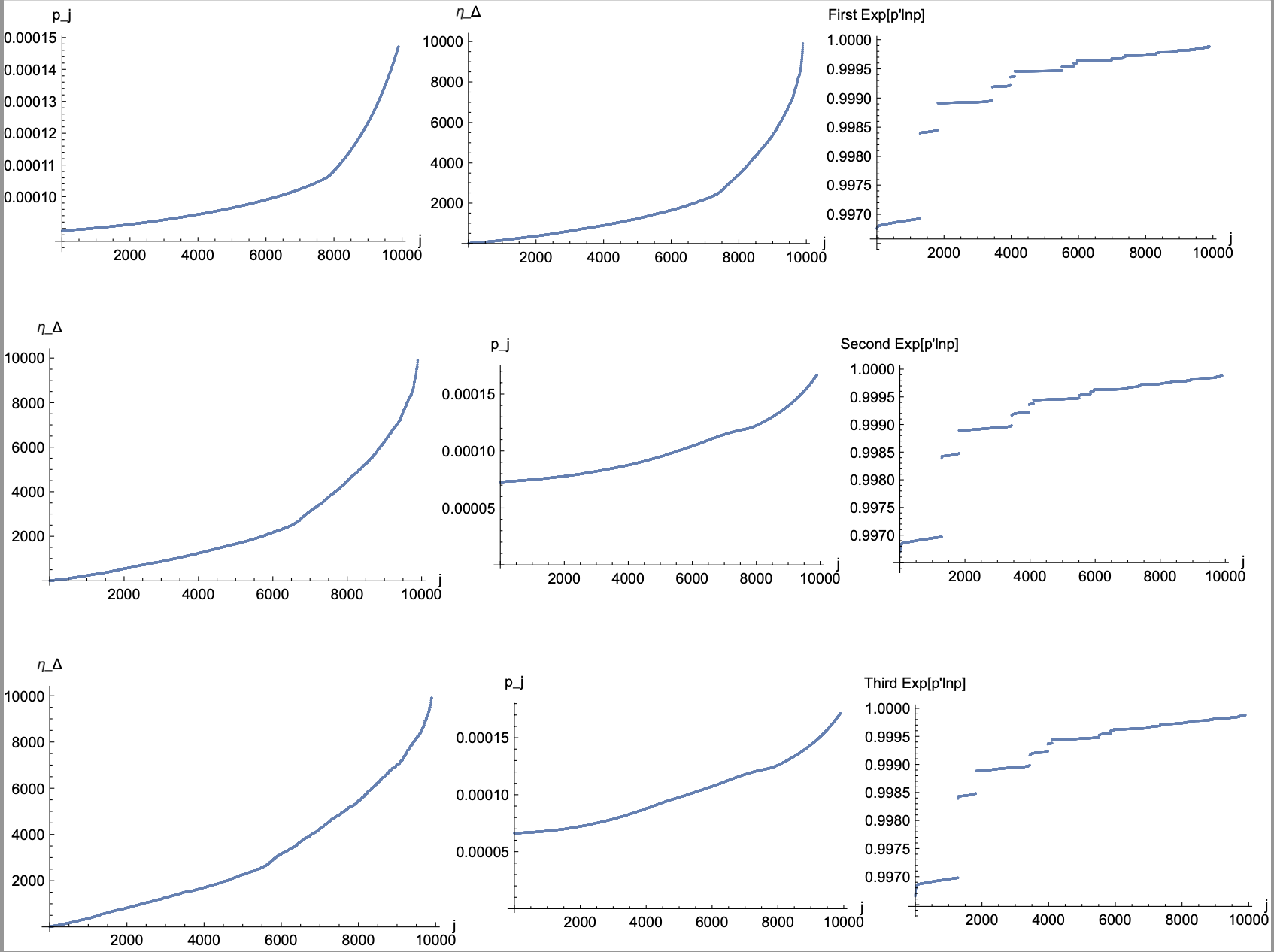
Figure 4: The first, second, and third rows show the three times of learning process using the self-attention method. The learnable parameters are automatically modified after each iteration. The first, second, and third columns are the predicted probability distributions, resulting $\eta_{\Delta}$-spectrums, and the $p_{i}^{p_{i}}$-spectrum which plays the role of loss function here to better identify the accuracy after each step.

Figure 5: Schematic diagram for the aglorithm. The black solid arrows stands the multiple operation. The red solid arrows stands the infinitely summation operation as shown by the formula within the red box. The black dashed arrows stands the operation of times $(-1)$ (becomes the negative one), and the blue line arrows of inverse operation ($F\rightarrow F^{(}-1)$). The six purple boxs within the orange box are the operations acting on the auxiliary function $H_{0}$. Each quantities can be expressed by the multiplication by all the quantities connected to it by an arrow (except the green arrows). The green arrows only indicating the results after the corresponding operations, e.g., $\lim_{k\rightarrow\infty}H_{0}$ and $I$ turn to teh same result after the derivative operation $\partial_{[K]}$ with the variable $[K]=k^{+}$ and $[K]=k$, respectively, as indicated near the corresponds green arrows.

References

- [1] Wu C H. Statistic behaviors of gauge-invariance-dominated 1D chiral current random model[J]. arXiv preprint arXiv:2207.07821, 2022.
- [2] Alexandrov A S. Transition from Fermi liquid to charged Bose liquid: A possible explanation of the isotope shift in high-T c oxides[J]. Physical Review B, 1992, 46(22): 14932.
- [3] Gu Y, Qi X L, Stanford D. Local criticality, diffusion and chaos in generalized Sachdev-Ye-Kitaev models[J]. Journal of High Energy Physics, 2017, 2017(5): 1-37.
- [4] Kohstall C, Zaccanti M, Jag M, et al. Metastability and coherence of repulsive polarons in a strongly interacting Fermi mixture[J]. Nature, 2012, 485(7400): 615-618.
- [5] Chowdhury D, Werman Y, Berg E, et al. Translationally invariant non-fermi-liquid metals with critical fermi surfaces: Solvable models[J]. Physical Review X, 2018, 8(3): 031024.
- [6] Culcer D. Linear response theory of interacting topological insulators[J]. Physical Review B, 2011, 84(23): 235411.
- [7] Sears V F, Svensson E C, Martel P, et al. Neutron-Scattering Determination of the Momentum Distribution and the Condensate Fraction in Liquid He 4[J]. Physical Review Letters, 1982, 49(4): 279.
- [8] Schick M. Two-dimensional system of hard-core bosons[J]. Physical Review A, 1971, 3(3): 1067.
- [9] Field B, Levinsen J, Parish M M. Fate of the Bose polaron at finite temperature[J]. Physical Review A, 2020, 101(1): 013623.
- [10] Christensen R S, Levinsen J, Bruun G M. Quasiparticle properties of a mobile impurity in a Bose-Einstein condensate[J]. Physical review letters, 2015, 115(16): 160401.
- [11] Allen S, Tremblay A M S. Nonperturbative approach to the attractive Hubbard model[J]. Physical Review B, 2001, 64(7): 075115.
- [12] Sedrakyan T A, Efetov K B. Supersymmetry method for interacting chaotic and disordered systems: The Sachdev-Ye-Kitaev model[J]. Physical Review B, 2020, 102(7): 075146.
- [13] Gu Y, Kitaev A, Sachdev S, et al. Notes on the complex Sachdev-Ye-Kitaev model[J]. Journal of High Energy Physics, 2020, 2020(2): 1-74.
- [14] Lantagne-Hurtubise é, Li C, Franz M. Family of Sachdev-Ye-Kitaev models motivated by experimental considerations[J]. Physical Review B, 2018, 97(23): 235124.
- [15] Pikulin D I, Franz M. Black hole on a chip: proposal for a physical realization of the Sachdev-Ye-Kitaev model in a solid-state system[J]. Physical Review X, 2017, 7(3): 031006.
- [16] Sachdev S. Bekenstein-Hawking entropy and strange metals[J]. Physical Review X, 2015, 5(4): 041025.
- [17] Buterakos D, Sarma S D. Coupled electron-impurity and electron-phonon systems as trivial non-Fermi liquids[J]. Physical Review B, 2019, 100(23): 235149.
- [18] Mahajan R, Barkeshli M, Hartnoll S A. Non-Fermi liquids and the Wiedemann-Franz law[J]. Physical Review B, 2013, 88(12): 125107.
- [19] Cha P, Patel A A, Gull E, et al. Slope invariant T-linear resistivity from local self-energy[J]. Physical Review Research, 2020, 2(3): 033434.
- [20] Xu C. Gapless bosonic excitation without symmetry breaking: An algebraic spin liquid with soft gravitons[J]. Physical Review B, 2006, 74(22): 224433.
- [21] Chen-Huan WU. SYK behaviors generated by on-site Hubbard-type four-fermion on-site random interactions and the related phase transitions. arXiv: 2105.12844.
- [22] Graser S, Maier T A, Hirschfeld P J, et al. Near-degeneracy of several pairing channels in multiorbital models for the Fe pnictides[J]. New Journal of Physics, 2009, 11(2): 025016.
- [23] Patel A A, Lawler M J, Kim E A. Coherent superconductivity with a large gap ratio from incoherent metals[J]. Physical review letters, 2018, 121(18): 187001.
- [24] Pikulin D I, Franz M. Black hole on a chip: proposal for a physical realization of the Sachdev-Ye-Kitaev model in a solid-state system[J]. Physical Review X, 2017, 7(3): 031006.
- [25] Wang Y. Solvable strong-coupling quantum-dot model with a non-Fermi-liquid pairing transition[J]. Physical review letters, 2020, 124(1): 017002.
- [26] Chen A, Ilan R, De Juan F, et al. Quantum holography in a graphene flake with an irregular boundary[J]. Physical review letters, 2018, 121(3): 036403.
- [27] Patel A A, Sachdev S. Critical strange metal from fluctuating gauge fields in a solvable random model[J]. Physical Review B, 2018, 98(12): 125134.
- [28] You Y Z, Ludwig A W W, Xu C. Sachdev-Ye-Kitaev model and thermalization on the boundary of many-body localized fermionic symmetry-protected topological states[J]. Physical Review B, 2017, 95(11): 115150.
- [29] Hu X, Pajerowski D M, Zhang D, et al. Freezing of a Disorder Induced Spin Liquid with Strong Quantum Fluctuations[J]. Physical Review Letters, 2021, 127(1): 017201.
- [30] Merz F, Chalker J T. Negative scaling dimensions and conformal invariance at the Nishimori point in the J random-bond Ising model[J]. Physical Review B, 2002, 66(5): 054413.
- [31] Levy R, Clark B K. Entanglement Entropy Transitions with Random Tensor Networks[J]. arXiv preprint arXiv:2108.02225, 2021.
- [32] Bi Z, Jian C M, You Y Z, et al. Instability of the non-Fermi-liquid state of the Sachdev-Ye-Kitaev model[J]. Physical Review B, 2017, 95(20): 205105.
- [33] Skinner B, Ruhman J, Nahum A. Measurement-induced phase transitions in the dynamics of entanglement[J]. Physical Review X, 2019, 9(3): 031009.
- [34] Ikegaya S, Kobayashi S, Asano Y. Symmetry conditions of a nodal superconductor for generating robust flat-band Andreev bound states at its dirty surface[J]. Physical Review B, 2018, 97(17): 174501.
- [35] Konig E J, Ostrovsky P M, Protopopov I V, et al. Metal-insulator transition in two-dimensional random fermion systems of chiral symmetry classes[J]. Physical Review B, 2012, 85(19): 195130.
- [36] Wei C, Sedrakyan T A. Optical lattice platform for the Sachdev-Ye-Kitaev model[J]. Physical Review A, 2021, 103(1): 013323.
- [37] Iyoda E, Katsura H, Sagawa T. Effective dimension, level statistics, and integrability of Sachdev-Ye-Kitaev-like models[J]. Physical Review D, 2018, 98(8): 086020.
- [38] Tracy C A, Widom H. The distributions of random matrix theory and their applications[J]. New trends in mathematical physics, 2009: 753-765.
- [39] Dumitriu I, Edelman A. Matrix models for beta ensembles[J]. Journal of Mathematical Physics, 2002, 43(11): 5830-5847.