An Einstein-Podolsky-Rosen argument based on weak forms of local realism not falsifiable by GHZ or Bell experiments

Abstract

The Einstein-Podolsky-Rosen (EPR) paradox gives an argument for the incompleteness of quantum mechanics based on the premises of local realism. A general view is that the argument is compromised, because EPR’s premises are falsified by Greenberger-Horne-Zeilinger (GHZ) and Bell experiments. In this paper, we present an EPR argument based on premises not falsifiable by these experiments. First, we propose macroscopic EPR and GHZ experiments using spins $\hat{S}_{\theta}$ defined by two macroscopically distinct states. The analyzers that realize the unitary operations $U_{\theta}$ determining the measurement settings $\theta$ are nonlinear devices known to create macroscopic superposition states. We note two definitions of macroscopic realism (MR). For a system with two macroscopically distinct states available to it, MR posits a predetermined outcome for a measurement $\hat{S}_{\theta}$ distinguishing between the states. Deterministic macroscopic realism (dMR) posits MR for the system defined prior to the interaction $U_{\theta}$ being carried out. Weak macroscopic realism (wMR) posits MR for the system after $U_{\theta}$, at the time $t_{f}$ $-$ when the system is prepared with respect to the measurement basis, ready for a final “pointer” measurement and readout. For this system, wMR posits that the outcome of $\hat{S}_{\theta}$ is determined, and not changed by interactions that might occur at a remote system $B$. The premise wMR also posits that if the outcome for $\hat{S}_{\theta}^{A}$ of a system $A$ can be predicted with certainty by a “pointer” measurement on the system $B$ defined at time $t_{f}^{B}$ after the unitary interaction that fixes the setting at $B$, then the outcome for $\hat{S}_{\theta}^{A}$ is determined for $A$ at this time $t_{f}^{B}$, regardless of whether the unitary interaction required to fix the setting as $\theta$ has taken place at $A$. We show that the GHZ predictions negate dMR but are consistent with wMR. Yet, an EPR paradox arises based on wMR. As considered by Schrödinger, it is possible to measure two complementary spins of system $A$ simultaneously, “one by direct, the other by indirect measurement”: If we assume wMR, then at time $t_{f}=t_{f}^{B}$, the outcomes of the two spins are both determined. We revisit the original EPR paradox and find a similar result: An EPR argument can be based on a weak contextual form of local realism (wLR) not falsifiable by GHZ or Bell tests.

I Introduction

In their argument of 1935, Einstein-Podolsky-Rosen (EPR) introduced premises, based on local realism, which if valid suggested quantum mechanics to be an incomplete description of physical reality epr . The argument considered two separated particles with correlated positions and anticorrelated momenta. The correlations imply that the outcome of a measurement of either position or momentum could be inferred with certainty for one particle, by an experimentalist making the appropriate measurement on the second particle. Assuming there is no disturbance to the first particle by the experimentalist’s actions, EPR argued from their premises that the position and momentum of the first particle are both simultaneously precisely determined prior to measurement, thereby creating an inconsistency with any quantum-state description for the localised particle.

Bell later proved that all local realistic theories could be falsified by quantum predictions bell-1969 ; bell-cs-review ; bell-1971 ; chsh ; bell-brunner-rmp . Moreover, Greenberger-Horne-Zeilinger (GHZ) ghz-1 ; mermin-ghz ; ghz-amjp ; clifton-ghz gave a falsification of EPR’s premises in an “all or nothing” situation. Bell and GHZ predictions have been experimentally verified ghz-pan ; ghz-exp-Bou . Consequently, the EPR paradox is most often regarded as an illustration of the incompatibility between local realism and quantum mechanics, rather than as a valid argument for the incompleteness of quantum mechanics epr-rmp ; mermin-ghz .

In this paper, we present a different perspective on the EPR paradox. We first propose a test of local realism versus quantum mechanics in a macroscopic GHZ set-up, where realism refers to a system being in one or other of two macroscopically distinct states. This provides a way to falsify local realism at a macroscopic level. Given such a falsification may raise questions for the interpretation of quantum measurement legggarg-1 ; s-cat-1935 , we then examine carefully the definitions of macroscopic realism, showing that a less restrictive definition of macroscopic realism is not falsified by GHZ or Bell experiments. This leads to a second conclusion: A modified EPR argument that quantum mechanics is incomplete can be given, based on an alternative and (arguably) nonfalsifiable premise.

Specifically, we show how the GHZ and EPR paradoxes can be realised for macroscopic qubits, where all relevant measurements $\hat{S}_{\theta}$ distinguish between two macroscopically distinct states. The EPR paradox is presented as Bohm’s version Bohm ; bohm-aharonov ; aspect-Bohm which examines two spatially-separated entangled spin-$1/2$ systems. The macroscopic version is a direct mapping of the original paradox, where a spin $|\uparrow\rangle$ and $|\downarrow\rangle$ is realised as two macroscopically distinct states, such as coherent states $|\alpha\rangle$ and $|-\alpha\rangle$, or collective multimode spin states $\prod_{k=1}^{N}|\uparrow\rangle_{k}$ and $\prod_{k=1}^{N}|\downarrow\rangle_{k}$. The necessary unitary transformations $U_{\theta_{i}}$ which determine the measurements settings $\theta_{i}$ for each system $i$ are realised by nonlinear interactions, or CNOT gates.

Leggett and Garg gave a definition of macroscopic realism (MR) for a system “with two or more macroscopically distinct states available to it”: MR asserts that the system “will at all times be in one or other of those states” legggarg-1 . Following previous work, we note different definitions are possible manushan-bell-cat-lg ; delayed-choice-cats . Deterministic macroscopic (local) realism (dMR) asserts there is a predetermined value $\lambda$ for the outcome of a measurement $S$ that will distinguish between the macroscopically distinct states. Locality is implied, since it is assumed that this value is not affected by spacelike-separated interactions or events.

However, the EPR-Bohm, Bell and GHZ experiments require choices of measurement settings $\theta_{i}$ at each site $i$, the choice establishing which spin component $S_{\theta_{i}}$ will be measured. This leads to different definitions of MR. The measurement basis is determined by the setting of a physical device (analogous to a Stern-Gerlach analyzer) which realizes a unitary operation $U_{\theta_{i}}=e^{-iH_{\theta_{i}}t/\hbar}$ where $H_{\theta_{i}}$ is the interaction Hamiltonian. After the interaction $U_{\theta_{i}}$ at a site $i$, there is a final stage of measurement that includes an irreversible coupling to an environment to give a readout of the spin $S_{\theta_{i}}$. We refer to this final stage as the “pointer measurement”.

In the macroscopic experiments we propose, the system after the selected interactions $U_{\theta_{i}}$ is in a superposition of macroscopically distinct states which have definite values for the outcomes $S_{\theta_{i}}$. Weak macroscopic realism (wMR) posits that each system $i$ prepared at a time $t_{f_{i}}$ after the interaction $U_{\theta_{i}}$ can be ascribed a predetermined value $\lambda_{\theta_{i}}$ for the final pointer part of the measurement $\hat{S}_{\theta_{i}}$, which will distinguish between the macroscopic states.

The premise wMR posits not only a weak form of realism, but also a weak form of locality. Consider the local system $i$ prepared at the time $t_{f_{i}}$ for the pointer measurement: There is no disturbance to the value $\lambda_{\theta_{i}}$ for the pointer measurement from interactions that might occur at a spacelike-separated site; nor from the pointer measurement (if it happened to be carried out) to a spacelike-separated system. In such a model, we will show that the nonlocal effects contributing to the GHZ and Bell contradictions with local realism emerge when there are further unitary interactions occurring at both sites.

The premise of deterministic local macroscopic realism (dMR) is similar to EPR and Bell’s form of local realism, because the premise applies to the system as it exists prior to the unitary interactions $U_{\theta_{i}}$. The macroscopic GHZ set-up hence enables an “all or nothing” falsification of dMR, which supports previous work revealing dMR to be falsifiable by macroscopic Bell tests macro-bell-lg ; manushan-bell-cat-lg ; delayed-choice-cats ; macro-bell-jeong ; wigner-friend-macro ; bell-contextual .

The main result of this paper is that weak macroscopic realism (wMR) is not falsified by the GHZ or Bell set-ups. Yet, an EPR-type argument can be put forward based on wMR. The argument applies to the EPR setup considered by Schrödinger, where two noncommuting observables are measured simultaneously “one by a direct, the other by indirect measurement” sch-epr-exp-atom ; s-cat-1935 . In our paper, the EPR-Bohm gedanken experiment is examined at the time $t_{f}$ after the unitary interactions $U_{\theta_{i}}$ have been carried out at each site, in order to measure spin $S_{z}$ of one system and $S_{y}$ of the other. The premise wMR posits a predetermined value for the pointer measurement of $S_{z}$ of the first system, since it can be shown to have two “macroscopically distinct states available to it” (with respect to the measurement basis $S_{z}$). But also for the EPR-Bohm state, the outcome for $S_{y}$ can be inferred for the first system by a pointer measurement on the other. Hence, wMR posits simultaneous precise values for both $S_{z}$ and $S_{y}$. This is not consistent with a local quantum state, the Pauli spin variances being constrained by $(\Delta\sigma_{z})^{2}+(\Delta\sigma_{y})^{2}\geq 1$ hofmann-take , which leads to the paradox. It is important to note that there is no actual violation of the uncertainty principle, because the quantum state defined at the time $t_{f}$ is different to the quantum state defined after the further interaction $U_{\theta^{\prime}_{i}}^{A}$ necessary to change the measurement setting from $z$ to $y$ at $A$.

The results motivate us to revisit the original microscopic EPR-Bohm paradox, and to demonstrate an EPR argument based on a weak contextual form of local realism (wLR), which we show is not falsified by GHZ or Bell set-ups. The definitions of wMR and wLR are both contextual, being defined for the system with a specified measurement basis. The weaker assumptions are motivated by Bohr’s criticism of EPR’s 1935 paper bell-cs-review ; bohr-epr . Clauser and Shimony state that “[Bohr’s] argument is that when the phrase ‘without in any way disturbing the system’ is properly understood, it is incorrect to say that system 2 is not disturbed by the experimentalist’s option to measure $a$ rather than $a^{\prime}$ on system 1.” This suggests that after the experimentalist’s option to measure say the spin component $a$, there is reason to justify no disturbance, the nonlocality stemming from the unitary interactions giving the options. We explain how wLR may be implied by wMR, by considering the system at the time of the reversible coupling to a macroscopic meter.

The layout of the paper is as follows. In Section II, we outline the definitions of local realism and macroscopic realism used in this paper. In Section III, we review the original EPR-Bohm and GHZ paradoxes, giving in Section IV the modified EPR-Bohm paradox based on the premise of wLR. In Sections V and VII, we present the proposals for macroscopic EPR-Bohm and GHZ paradoxes using cat states. Conclusions drawn from these paradoxes are given in Sections VI and VIII. The macroscopic GHZ paradox falsifies dMR, but shows consistency with wMR. Similarly, the GHZ paradox is consistent with wLR. In Section IX, we demonstrate consistency of wLR (and wMR) with violations of Bell inequalities. Further tests of wMR and wLR are devised in Section X.

II Definitions

We formalize the definitions of local realism and macroscopic realism relevant to this paper. Several different definitions are introduced. The difference between the definitions is clarified, once we recognise that there are two stages to a spin measurement $S_{\theta}$: First, there is the reversible measurement-setting stage involving a unitary interaction $U_{\theta}$ which determines the measurement setting $\theta$. Second, there is the stage that comes after, which includes a final irreversible readout of a meter. We refer to the later stage as the pointer [stage of] measurement.

Consider two separated spin-$1/2$ systems $A$ and $B$ prepared at time $t_{0}$ in the state $|\psi\rangle$. Local unitary interactions $U_{\theta}^{A}$ and $U_{\phi}^{B}$ prepare the systems for spin measurements $S_{\theta}^{A}$ and $S_{\phi}^{B}$. The $U_{\theta}$ are realised as reversible interactions of the system with a real device, such as a Stern-Gerlach analyzer or polarizing beam splitter, and are represented by a Hamiltonian $H_{\theta}$, where $U_{\theta}=e^{-iH_{\theta}t/\hbar}$. The $U_{\theta}$ takes place over a time interval $t$, and the states prior and after the interaction $U_{\theta}$ may therefore be regarded as different, in that they define the system at a different time. The state after the interaction at time $t_{f}$ is

$$|\psi(t_{f})\rangle=e^{-iH_{\theta}t_{f}/\hbar}|\psi\rangle$$ (1)

Specific examples are given in Sections IV and V, where we note that the “system” may include another (local) set of modes, or a meter that is originally decoupled to the spin system, in which case $|\psi\rangle$ is suitably defined. After the interaction $U$, the final irreversible stage of the measurement is made, which indicates the measurement outcome. This stage often involves a direct detection of a particle at a given location, as well as amplification and a coupling to a meter. The local system prepared after the interaction $U$ that fixes the measurement setting, but before the irreversible stage of the measurement, is considered to be prepared for the pointer measurement. The system is said to be prepared in the preferred basis, also referred to as the measurement, or pointer, basis.

A common realisation is the spin $1/2$ system $|\uparrow\rangle\equiv|1,0\rangle$ and $|\downarrow\rangle\equiv|0,1\rangle$ defined for two orthogonally polarized modes $a_{\pm}$. Here, $|n_{1},n_{2}\rangle\equiv|n_{1}\rangle_{+}|n_{2}\rangle_{-}$ where $|n\rangle_{\pm}$ is a number state for the mode $a_{\pm}$. A transformation $U_{\theta}$ can then be achieved with a polarizing beam splitter, with mode transformations ($\hat{a}_{\pm}$ are boson operators defining the modes)

$$\hat{c}_{+} = \hat{a}_{+}\cos\theta-\hat{a}_{-}\sin\theta$$

$$\hat{c}_{-} = \hat{a}_{+}\sin\theta+\hat{a}_{-}\cos\theta.$$ (2)

The $\hat{c}_{\pm}$ are boson operators for the outgoing modes emerging from the beam splitter. The interaction is described by the Hamiltonian $H_{\theta}=i\hbar k(\hat{a}_{+}\hat{a}_{-}^{\dagger}-\hat{a}_{+}^{\dagger}\hat{a}_{-})$ where $\theta=kt$. The choice $\theta=0$ ($\theta=\pi/4)$ corresponds to a measurement of $\sigma_{z}$ ($\sigma_{x}$). A single photon impinges on the beam splitter and is finally detected at one or other locations associated with the outgoing modes aspect-Bohm . The final detection and readout of the locations constitutes the pointer measurement.

More recently, an EPR experiment has been realised for pseudo-spin measurements in a BEC setting sch-epr-exp-atom . Here, the measurement setting is determined by an interaction of a field with a two-level atom, which forms the spin $1/2$ system.

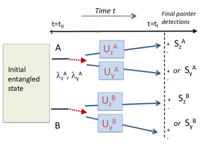
Figure 1: The set-up for an EPR-Bohm paradox. Two separated systems $A$ and $B$ are prepared in an entangled state $|\psi\rangle$ (Eq. (4)). A switch (red dashed arrow) gives the choice to measure either $S_{z}$ or $S_{y}$ for each of $A$ and $B$, by passing through an appropriately orientated analyzer symbolised by $U$ at each site. Here, $S_{z}$ and $S_{y}$ correspond to Pauli spins $\sigma_{z}$ and $\sigma_{y}$. EPR’s local realism asserts that because one can predict the result for $S_{z}$ (or $S_{y}$) at $A$ by measuring $S_{z}$ (or $S_{y}$) at $B$, the outcomes for $S_{z}$ and $S_{y}$ at $A$ are both predetermined, at the time $t_{0}$ (prior to the choices of measurement setting). The premises of macroscopic local realism and deterministic macroscopic realism apply when the outcomes $+$ and $-$ for both spins $S_{z}$ and $S_{y}$ are associated with macroscopically distinct states for the system at the time $t_{0}$.

II.1 Strong elements of reality: EPR’s Local realism and Macroscopic realism

II.1.1 EPR’s Local realism

The premises presented in the original 1935 argument given by EPR are based on the assumptions of local realism. The premises, which we refer to as EPR’s local realism (LR), are summarized as two Assertions for space-like separated systems, $A$ and $B$.

EPR’s Assertion LR (1): Realism

EPR’s reality criterion is: “If, without in any way disturbing a system, we can predict with certainty the value of a physical quantity, then there exists an element of physical reality corresponding to this physical quantity epr .”

This is interpreted as follows: “The "element of physical reality" is that predictable value, and it ought to exist whether or not we actually carry out the procedure necessary for its prediction, since that procedure in no way disturbs it mermin-ghz .” Hence, EPR Assertion LR (1) reads: If one can predict with certainty the outcome of a measurement $S$ on system $A$ without disturbing that system, then the outcome of the measurement is predetermined. The system $A$ can be ascribed a variable $\lambda^{A}$, the value of which gives the outcome for $S$ mermin-ghz .

EPR Assertion LR (2): No disturbance (Locality)

There is no disturbance to system $A$ from a spacelike-separated interaction or event (e.g. a measurement on system $B$).

The consequences of the two Assertions as applied to the EPR-Bohm set-up leads to the EPR-Bohm paradox (Section III). Consider the system of Figure 1: If the outcome of the measurement $S_{\theta}^{A}$ at $A$ can be predicted with certainty by a measurement at $B$, then the EPR Assertions imply the system $A$ at time $t_{0}$ can be ascribed a variable $\lambda_{\theta}^{A}$, the value of which gives the outcome of the measurement $S_{\theta}^{A}$. The assignment of the variable $\lambda_{\theta}^{A}$ can be made to the system $A$ regardless of the measurement device actually being prepared, either at $A$ or at $B$. In the Figure 1, this allows the assignment of both variables $\lambda_{z}^{A}$ and $\lambda_{y}^{A}$ to system $A$, at the time $t_{0}$, prior to the unitary interactions $U_{\theta}^{A}$ and $U_{\phi}^{B}$ that determine the measurement settings.

II.1.2 Macroscopic local realism and deterministic macroscopic realism

The assertions defining macroscopic local realism (MLR) are identical to those of EPR’s local realism, except that the assertions are weaker, being restricted to apply only to the subset of systems where the outcomes for all relevant measurements, $S_{\theta}^{A}$ and $S_{\phi}^{B}$, correspond to macroscopically distinct states of the system. This means that the systems upon which those measurements are made can be viewed as having two (or more) macroscopically distinct states available to them, so that the Leggett-Garg definition of macroscopic realism legggarg-1 can be applied, to separately posit deterministic macroscopic realism (dMR), as below. It would be argued that the assumption of realism is more robustly justified for macroscopically distinct states s-cat-1935 .

Assertion MLR (1a): EPR’s realism

This reads as for EPR Assertion LR (1). “If, without in any way disturbing a system, we can predict with certainty the value of a physical quantity, then there exists an element of physical reality corresponding to this physical quantity.”

Assertion dMR (1b): Leggett-Garg’s criterion for Macroscopic realism $-$ Deterministic macroscopic realism (dMR)

A system which has two or more macroscopically distinct states available to it can be ascribed a predetermined value $\lambda$ for the measurement $S$ that will distinguish between these states. The predetermined value $\lambda$ is not affected by spacelike-separated measurements (e.g. further unitary transformations $U_{\phi}$) that may occur at site $B$. Hence, locality is implied, which also follows from Assertion MLR(2) below.

Assertion MLR (2): No disturbance (Locality)

There is no macroscopic disturbance to system $A$ from a spacelike-separated interaction or event.

Similar to EPR’s local realism, deterministic macroscopic realism asserts there is a predetermined value $\lambda_{\theta}$ for the outcome of the measurement at the time $t_{0}$, for the system as it exists prior to, or irrespective of, the interaction $U_{\theta}$ (Figure 1).

II.2 Weak elements of reality: weak macroscopic realism and weak local realism

II.2.1 Weak macroscopic realism

Weak macroscopic realism (wMR) involves weaker (i.e. less restrictive) assumptions than macroscopic local realism. Macroscopic local realism implies wMR, but the converse is not true. The assertions for wMR are modified so that EPR’s local realism applies to the systems after the selection of the measurement settings, at time $t_{f}$ in the Figure 2.

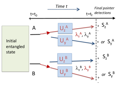
Figure 2: The assumption of weak local realism (wLR) gives rise to an EPR paradox: The set-up is for an EPR-Bohm paradox as in Figure 1. At time $t_{f}$, the measurement settings are set to $S_{z}^{A}$ and $S_{y}^{B}$, as indicated by the positions of the red dashed arrows. Weak local realism asserts that for the system $A$ at time $t_{f}$, after the unitary rotation $U_{z}^{A}$, the outcome for the final pointer measurement $S_{z}$ at $A$ is determined, given by the variable $\lambda_{z}^{A}$. Weak local realism also asserts that because one can predict the result for $S_{y}$ at $A$ by making a final pointer measurement $S_{y}$ at $B$, the outcome for $S_{y}$ at $A$ is also determined at time $t_{f}$ (after the rotation $U_{y}^{B}$ at $B$). This is despite that a further unitary evolution $U^{A}$ would be required at $A$ to perform the measurement $S_{y}^{A}$. This leads to the paradox. The premise of weak macroscopic realism applies similarly, assuming the outcomes $+$ and $-$ for the spins can be viewed as corresponding to macroscopically distinct states for the system at the time $t_{f}$.

Assertion wMR (1a): EPR’s criterion for realism

This assertion reads as for Assertion MLR (1a). “If, without in any way disturbing a system, we can predict with certainty the value of a physical quantity, then there exists an element of physical reality corresponding to this physical quantity epr .”

The conclusions from Assertion wMR (1a) will now be different from those of EPR, due to the modification of Assertion (2a) below. Suppose system $B$ at time $t_{f}$, after the unitary interaction $U_{\phi}^{B}$, is prepared for the pointer stage of measurement of spin $S_{\phi}^{B}$. Assertion wMR 2(a) asserts that there is no disturbance to system $A$ due to whether or not the pointer stage of measurement at $B$ actually takes place. The modification means that the prediction for the outcome of measurement $S$ at $A$, as based on a measurement at $B$, ensures a predetermination of the result at $A$ at the time $t_{f}$, provided the unitary interaction $U_{\phi}^{B}$ that fixes the measurement setting $\phi$ at $B$ has taken place.

The Assertion wMR (1a) can hence be rephrased: Consider the system of Figure 2: If the outcome of a measurement $S_{\theta}^{A}$ at $A$ can be predicted with certainty by a pointer measurement on the system at time $t_{f}$ at $B$, then there exists an element of physical reality corresponding to the outcome of $S_{\theta}^{A}$ at $A$. Thus, the system $A$ can be ascribed a hidden variable $\lambda_{\theta}^{A}$ that determines the outcome for $S_{\theta}^{A}$. This is true regardless of whether the pointer measurement at $B$ is actually carried out (because that would not disturb the system $A$), and regardless of whether the interaction $U^{A}$ at $A$ that fixes the measurement setting $\theta$ has actually been carried out at $A$ (and regardless of future unitary interactions at $A$). However, the predetermination is based on the system $B$ being prepared for a pointer measurement, and therefore only applies at the time $t_{f}$, when no further unitary interactions that would cause a change of measurement setting at $B$ have taken place.

Assertion wMR (1b): Macroscopic realism for the system prepared for the pointer measurement

Suppose a system $A$ that is prepared for the pointer measurement of $S$ can be considered to have two or more macroscopically distinct states available to it, where each of those states has a definite outcome for the pointer measurement. Weak macroscopic realism asserts that such a system can be ascribed a predetermined value $\lambda^{A}$ for the pointer measurement $S$ that will distinguish between these states.

The premise applies, so that the result of the pointer measurement for $S_{\theta}^{A}$ is predetermined at the time $t_{f}$, once the interaction $U_{\theta}^{A}$ determining the measurement setting at $A$ has taken place (Figure 2).

Assertion wMR (2a): Pointer locality: No disturbance from a pointer measurement

The pointer stage of a measurement gives no disturbance to a spacelike-separated system i.e. there is no disturbance to system $A$ from a pointer measurement on system $B$.

Assertion wMR (2b): Pointer locality: No disturbance to a pointer measurement

There is no disturbance to the predetermined value $\lambda^{A}$ for the pointer measurement at $A$ (as described in Assertion wMR (1b)) by spacelike-separated interactions or events (e.g. further unitary transformations $U_{\phi}^{B}$) that may occur at $B$.

The assertions when applied to EPR-Bohm set-up of Figure 2 will lead to an EPR-type paradox, as explained in Sections IV and V.

II.3 Weak local realism

The premise of weak local realism (wLR) is a weak form of local realism, which applies to the system prepared at time $t_{f}$ for the pointer measurement (Figure 2). This contrasts with definitions of local realism that apply to the system at time $t_{0}$, prior to the entire measurement process, and which can be falsified. It should be mentioned that weak local realism, as with weak macroscopic realism, does not exclude “nonlocality”, since, as we will see, these premises are consistent with the quantum predictions for Bell and GHZ experiments.

The assertions of wLR are as for weak macroscopic realism (wMR), except there is no longer the restriction that the outcomes correspond to macroscopically distinct states of the system being measured. A connection between wLR and wMR is given in the Section II.D. As with wMR, in this model, the pointer measurement constitutes a passive stage of the measurement.

We comment on the terminology local realism. The most general definition of local realism is given by Bell’s local hidden variable theories, also referred to as local realistic theories bell-cs-review . These theories allow for local interactions with local measurement devices, so that the value for the outcome of the measurement need not be predetermined (at time $t_{0}$ or $t_{f}$). This contrasts with the stricter definition, which we refer to as a non-contextual or deterministic local realism bell-cs-review , meaning the values for measurement outcomes are predetermined at the time $t_{0}$, prior to the entire measurement process including the unitary interactions $U$. However, general local realistic hidden variable theories imply EPR’s local realism. Moreover, for the EPR-Bohm system where the correlations between certain spin measurements are maximum, the local realistic theories also imply the stricter deterministic local realism, for spin measurements bell-1969 .

Generally speaking, however, we cannot assume wLR to be a “weaker” assumption than local realism, in the sense that it not necessarily a subset of those assumptions, since local realistic theories may allow non-passive interactions with the pointer measurement apparatus. To avoid confusion, we emphasize that weak local realism refers to a weaker version of the non-contextual deterministic form of local realism. In later Sections, we show that while all local realistic theories are ruled out by GHZ and Bell experiments, wLR theories are not, which motivates the terminology “weak”.

Assertion wLR (1a): EPR’s realism

The assertion is as for EPR Assertion LR (1). As with wMR, the conclusions drawn from this Assertion are impacted by Assertion (2a). Weak local realism asserts: If the outcome of the measurement $S_{\theta}^{A}$ at $A$ can be predicted with certainty at time $t_{f}$ by the final pointer stage of measurement at $B$ (the local dynamics $U$ of the measurement setting being already performed at $B$), then the system at $A$ at time $t_{f}$ can be ascribed a variable $\lambda_{\theta}^{A}$, the value of which gives the outcome of the measurement $S_{\theta}^{A}$. This is true regardless of whether the pointer measurement at $B$ is actually performed, and regardless of whether the unitary interaction $U_{\theta}^{A}$ has taken place at $A$, and regardless of any further unitary interactions at $A$ (Figure 2).

Assertion wLR (1b): Realism for the system prepared for the pointer measurement

The result of the pointer measurement for $S^{A}$ for system $A$ is predetermined (by a variable $\lambda^{A}$) once the local interaction $U_{\theta}^{A}$ for the measurement setting at $A$ has taken place.

Consider the system $A$ at time $t_{f}$, after the unitary rotation $U_{\theta}^{A}$. The system $A$ is prepared for the pointer stage of measurement of $S_{\theta}^{A}$, without the need for a further unitary rotation $U$. The premise wLR asserts that the system $A$ at time $t_{f}$ can be ascribed by a hidden variable $\lambda_{\theta}^{A}$ with value $+1$ or $-1$, that value determining the outcome of the pointer measurement for $S_{\theta}^{A}$ at $A$, if that pointer stage of measurement were to be carried out on the prepared state. In accordance with Assertion (2b), the predetermined value $\lambda_{\theta}^{A}$ is not affected by spacelike-separated events (e.g. further unitary transformations $U_{\phi}$) that may occur at $B$.

Assertion wLR (2a): Pointer locality: No disturbance from a pointer measurement

The assertion reads as for Assertion wMR (2a).

Assertion wLR (2b): Pointer locality: No disturbance to a pointer measurement

The assertion reads as for Assertion wMR (2b).

The Assertion wLR (1b) which asserts realism is less convincing for a microscopic system than for a macroscopic system, and might seem to contradict the results of Bell’s theorem. We later show that wLR is not contradicted by the Bell or GHZ predictions. The assertions when applied to the set-up of Figure 2 will nonetheless lead to an EPR-type paradox, as explained in Section IV.

II.4 Link between wLR and wMR

At first glance, weak local realism (wLR) is seen to be a stronger assumption than weak macroscopic realism (wMR), meaning it is a more restrictive (less convincing) assumption. However, if the time $t_{f}$ is carefully specified, we show that wLR can be justified by wMR.

Consider the system at time $t_{f}$ after the unitary rotations $U_{\theta}^{A}$ and $U_{\phi}^{B}$ that determine the measurement settings, say $\theta$ and $\phi$, respectively at $A$ and $B$. At this stage, or later, in the measurement process, there is a coupling of each local system to a macroscopic meter, via an interaction $H_{M}$. The final state after coupling is of the form

$$|\psi_{M}\rangle = c_{1}|p_{+}\rangle_{A}|\uparrow\rangle_{\theta}|p_{-}\rangle_{B}|\downarrow\rangle_{\phi}+c_{2}|p_{-}\rangle_{A}|\downarrow\rangle_{\theta}|p_{+}\rangle_{B}|\uparrow\rangle_{\phi}$$

$$+c_{3}|p_{+}\rangle_{A}|\uparrow\rangle_{\theta}|p_{+}\rangle_{B}|\uparrow\rangle_{\phi}+c_{4}|p_{-}\rangle_{A}|\downarrow\rangle_{\theta}|p_{-}\rangle_{B}|\downarrow\rangle_{\phi}$$

where $c_{i}$ are probability amplitudes, and $|p_{+}\rangle_{A/B}$ and $|p_{-}\rangle_{A/B}$ are macroscopic states for the pointer of the meter, indicating Pauli spin outcomes of $+1$ and $-1$ respectively, at $A$ and $B$. We see that $|\psi_{M}\rangle$ is a macroscopic superposition state. Weak macroscopic realism implies predetermined values $\lambda_{M}^{A}$ and $\lambda_{M}^{B}$ for the outcomes of measurements on the meter systems $-$ the pointers are already in some kind of definite state that will indicate the result of the measurement to be either “spin up” or “spin down”.

In view of the correlation, it can then be argued that the systems $A$ and $B$ (which may be microscopic) are similarly specified to be in states with a definite outcome for the final measurement of spin components $\theta$ and $\phi$, respectively. The interaction $H_{M}$ is reversible, and hence the definition of wLR can be rephrased to apply to the system at the time $t_{f}$ where it is assumed the stage of the measurement that couples each system to a meter has already occurred, just after or in association with the unitary interactions $U_{\theta}^{A}$ and $U_{\phi}^{B}$. Due to the reversibility of $H_{M}$, this does not change the results of the paper.

III EPR-Bohm and GHZ paradoxes

III.1 Bohm’s version of the EPR paradox

Bohm generalized the EPR paradox to spin measurements by considering two spatially separated spin $1/2$ particles prepared in the Bell state Bohm ; bell-1969

$$|\psi_{B}\rangle = \frac{1}{\sqrt{2}}(|\uparrow\rangle_{z}|\downarrow\rangle_{z}-|\downarrow\rangle_{z}|\uparrow\rangle_{z}).$$ (4)

The particles and their respective sites are denoted by $A$ and $B$. Here $|\uparrow\rangle_{z}$ and $|\downarrow\rangle_{z}$ are the eigenstates of the $z$ component $\sigma_{z}$ of the Pauli spin $\overrightarrow{\sigma}=(\sigma_{x},\sigma_{y},\sigma_{z})$, with eigenvalues $+1$ and $-1$ respectively. We use the standard notation, where the first and second states of the product $|\uparrow\rangle|\downarrow\rangle$ refer to the states of particle $A$ and particle $B$ respectively. The spin operators for the two particles are distinguished by superscripts e.g. $\sigma_{z}^{A}$ and $\sigma_{z}^{B}$.

III.1.1 A two-spin version

From (4), it is clear that the outcomes of spin-$z$ measurements on each particle are anticorrelated. Similarly, we may measure the component $\sigma_{y}$ of each particle. To predict the outcomes, we transform the state into the $y$ basis, noting the transformation

$$|\uparrow\rangle_{y} = \frac{1}{\sqrt{2}}(|\uparrow\rangle_{z}+i|\downarrow\rangle_{z})$$

$$|\downarrow\rangle_{y} = \frac{1}{\sqrt{2}}(|\uparrow\rangle_{z}-i|\downarrow\rangle_{z})$$ (5)

where $|\uparrow\rangle_{y}$ and $|\downarrow\rangle_{y}$ are the eigenstates of $\sigma_{y}$, with respective eigenvalues $+1$ and $-1$. Hence we find $|\uparrow\rangle_{z}=(|\uparrow\rangle_{y}+|\downarrow\rangle_{y})/\sqrt{2}$ and $|\downarrow\rangle_{z}=-i(|\uparrow\rangle_{y}-|\downarrow\rangle_{y})/\sqrt{2}$. The state becomes in the new basis

$$|\psi_{B}\rangle = \frac{i}{\sqrt{2}}(|\uparrow\rangle_{y}|\downarrow\rangle_{y}-|\downarrow\rangle_{y}|\uparrow\rangle_{y}).$$ (6)

Denoting the respective measurements at each site by $\sigma_{y}^{A}$ and $\sigma_{y}^{B}$, we see that the spin-$y$ outcomes at $A$ and $B$ are also anticorrelated.

An EPR-Bohm paradox follows from the following argument (Figure 1). By making a measurement of $\sigma_{z}^{B}$ on particle $B$, the outcome for the measurement $\sigma_{z}^{A}$ on particle $A$ is known with certainty. EPR present their Assertions of local realism (LR) epr , summarized in Section II.A.1. Invoking EPR Assertion LR (2) that there is no disturbance to system $A$ due to the measurement at $B$, EPR’s Assertion LR (1) therefore implies system $A$ can be ascribed a hidden variable $\lambda_{z}^{A}$ mermin-ghz , which predetermines the outcome for the measurement $\sigma_{z}^{A}$ should that measurement be performed. However, the outcomes at $A$ and $B$ are also anticorrelated for measurements of $\sigma_{y}$ at both sites. The assumption of EPR’s premises therefore ascribes two hidden variables $\lambda_{z}^{A}$ and $\lambda_{y}^{A}$ to the system $A$, which simultaneously predetermine the outcome of either $\sigma_{z}$ or $\sigma_{y}$ at $A$, should either measurement be performed. This description is not compatible with any quantum wavefunction $|\psi\rangle$ for the spin $1/2$ system $A$. The conclusion is that if EPR’s local realism is valid, then quantum mechanics gives an incomplete description of physical reality.

The above conclusions draw on the assumption that the subsystem $A$ is described quantum mechanically as a spin $1/2$ system. For such a system, the Pauli spin variances defined by $(\Delta\sigma_{i})^{2}=\langle\sigma_{i}^{2}\rangle-\langle\sigma_{i}\rangle^{2}$ satisfy the uncertainty relation $(\Delta\sigma_{x})^{2}+(\Delta\sigma_{y})^{2}+(\Delta\sigma_{z})^{2}\geq 2$ hofmann-take . Since $(\Delta\sigma_{z})^{2}\leq 1$, this implies hofmann-take

$$(\Delta\sigma_{y})^{2}+(\Delta\sigma_{z})^{2}\geq 1.$$ (7)

For a quantum state description of the system $A$, the values of $\sigma_{y}$ and $\sigma_{z}$ cannot be simultaneously precisely defined. A realisation has been given for two spin $1/2$ particles (photons) which showed near-perfect correlation for both of two orthogonal spins (orthogonal linear polarizations), for a subensemble where both photons are detected aspect-Bohm .

III.1.2 Three-spin version

A stricter argument not dependent on the assumption of a spin $1/2$ system is possible, if the experimentalist can measure the correlation of all three spin components Bohm ; epr-rmp ; bohm-test-uncertainty . Consider the spin-$x$ measurements $\sigma_{x}^{A}$ and $\sigma_{x}^{B}$. The eigenstates of $\sigma_{x}$ are

$$|\uparrow\rangle_{x} = \frac{1}{\sqrt{2}}(|\uparrow\rangle_{z}+|\downarrow\rangle_{z})$$

$$|\downarrow\rangle_{x} = \frac{1}{\sqrt{2}}(|\uparrow\rangle_{z}-|\downarrow\rangle_{z}).$$ (8)

The state (4) becomes in the spin-$x$ basis

$$|\psi_{B}\rangle = \frac{1}{\sqrt{2}}(|\downarrow\rangle_{x}|\uparrow\rangle_{x}-|\uparrow\rangle_{x}|\downarrow\rangle_{x}).$$ (9)

The spin-$x$ outcomes at $A$ and $B$ are also anticorrelated. According to the EPR premises, it is therefore possible to assign a hidden variable $\lambda_{x}^{A}$ to the subsystem $A$ that predetermines the outcome of the measurement $\sigma_{x}^{A}$. Hence, local realism implies that the system $A$ would at any time be described by three precise values, $\lambda_{x}^{A}$, $\lambda_{y}^{A}$ and $\lambda_{z}^{A}$, which predetermine the outcomes of measurements $\sigma_{x}$, $\sigma_{y}$ and $\sigma_{z}$ respectively. Each of $\lambda_{x}$, $\lambda_{y}$ and $\lambda_{z}$ has the value $+1$ or $-1$ . Since always $|\lambda_{z}^{A}|=1$, such a hidden variable description cannot be given by a local quantum state $|\psi\rangle$ of $A$, as this would be a violation of the quantum uncertainty relation

$$\Delta\sigma_{x}\Delta\sigma_{y}\geq|\langle\sigma_{z}\rangle|,$$ (10)

which applies to all quantum states. Hence, we arrive at an EPR paradox, where local realism implies an inconsistency with the completeness of quantum mechanics.

III.2 GHZ paradox

The Greenberger-Horne-Zeilinger (GHZ) argument shows that local realism can be falsified, if quantum mechanics is correct ghz-1 ; mermin-ghz ; ghz-amjp ; clifton-ghz . The GHZ state

$$|\psi_{GHZ}\rangle = \frac{1}{\sqrt{2}}(|\uparrow\rangle_{z}|\uparrow\rangle_{z}|\uparrow\rangle_{z}-|\downarrow\rangle_{z}|\downarrow\rangle_{z}|\downarrow\rangle_{z})$$ (11)

involves three spatially separated spin $1/2$ particles, $A$, $B$ and $C$. We denote the Pauli spin measurement $\sigma_{\theta}$ at the site $J\in\{A,B,C\}$ by $\sigma_{\theta}^{J}$. Consider measurements of $\sigma_{x}$ at each site. To obtain the predicted outcomes, we rewrite in the spin-$x$ basis. The GHZ state becomes

$$|\psi_{GHZ}\rangle = \frac{1}{\sqrt{2}}(|\downarrow\rangle_{x}|\uparrow\rangle_{x}|\uparrow\rangle_{x}+|\uparrow\rangle_{x}|\downarrow\rangle_{x}|\uparrow\rangle_{x}$$ (12)

$$+|\uparrow\rangle_{x}|\uparrow\rangle_{x}|\downarrow\rangle_{x}+|\downarrow\rangle_{z}|\downarrow\rangle_{z}|\downarrow\rangle_{z}).$$

From this we see $\langle\sigma_{x}^{A}\sigma_{x}^{B}\sigma_{x}^{C}\rangle=-1.$ Now we also consider the measurement $\sigma_{x}^{A}\sigma_{y}^{B}\sigma_{y}^{C}$ on the system in the GHZ state. The GHZ state in the spin-$y$ basis is:

$$|\psi_{GHZ}\rangle = \frac{1}{\sqrt{2}}(|\uparrow\rangle_{x}|\uparrow\rangle_{y}|\uparrow\rangle_{y}+|\downarrow\rangle_{x}|\downarrow\rangle_{y}|\uparrow\rangle_{y}$$ (13)

$$+|\downarrow\rangle_{x}|\uparrow\rangle_{y}|\downarrow\rangle_{y}+|\uparrow\rangle_{x}|\downarrow\rangle_{y}|\downarrow\rangle_{y}).$$

This shows $\langle\sigma_{x}^{A}\sigma_{y}^{B}\sigma_{y}^{C}\rangle=1.$ Similarly, $\langle\sigma_{y}^{A}\sigma_{x}^{B}\sigma_{y}^{C}\rangle=1$ and $\langle\sigma_{y}^{A}\sigma_{y}^{B}\sigma_{x}^{C}\rangle=1$.

The GHZ argument is well known. The outcome for $\sigma_{x}$ at $A$ can be predicted with certainty by performing measurements $\sigma_{x}^{B}$ and $\sigma_{x}^{C}$. The measurements do not disturb the system $A$ because the measurements at $A$ and those at $B$ and $C$ are spacelike-separated events. Similarly, the outcome for $\sigma_{y}^{A}$ can be predicted, without disturbing the system $A$, by measurements of $\sigma_{y}^{B}$ and $\sigma_{x}^{C}$. Hence, there exist hidden variables $\lambda_{x}^{A}$ and $\lambda_{y}^{A}$ that can be simultaneously ascribed to system $A$, these variables predetermining the outcome for measurements $\sigma_{x}^{A}$ and $\sigma_{y}^{A}$ at $A$. The variables assume the values of $+1$ or $-1$. A similar argument can be made for particles $B$ and $C$. The contradiction with EPR’s local realism arises because the product $\lambda_{x}^{A}\lambda_{x}^{B}\lambda_{x}^{C}$ must equal $-1$, in order that the prediction $\langle\sigma_{x}^{A}\sigma_{x}^{B}\sigma_{x}^{C}\rangle=-1$ holds. Similarly, $\lambda_{x}^{A}\lambda_{y}^{B}\lambda_{y}^{C}=\lambda_{y}^{A}\lambda_{x}^{B}\lambda_{y}^{C}=\lambda_{y}^{A}\lambda_{y}^{B}\lambda_{x}^{C}=1$ in order that the prediction $\langle\sigma_{x}^{A}\sigma_{y}^{B}\sigma_{y}^{C}\rangle=\langle\sigma_{y}^{A}\sigma_{x}^{B}\sigma_{y}^{C}\rangle=\langle\sigma_{y}^{A}\sigma_{y}^{B}\sigma_{x}^{C}\rangle=1$ holds. Yet, we see algebraically that $\lambda_{x}^{A}\lambda_{x}^{B}\lambda_{x}^{C}=\lambda_{x}^{A}\lambda_{x}^{B}\lambda_{x}^{C}(\lambda_{y}^{B})^{2}(\lambda_{y}^{A})^{2}(\lambda_{y}^{C})^{2}$, and hence

$$\lambda_{x}^{A}\lambda_{x}^{B}\lambda_{x}^{C} = (\lambda_{x}^{A}\lambda_{y}^{B}\lambda_{y}^{C})(\lambda_{x}^{B}\lambda_{y}^{A}\lambda_{y}^{C})(\lambda_{x}^{C}\lambda_{y}^{B}\lambda_{y}^{A})$$ (14)

$$= 1$$

which gives a complete “all or nothing” contradiction. The conclusion is that local realism does not hold.

IV An EPR paradox based on weak local realism

An argument can be formulated that quantum mechanics is incomplete, based on the wLR premise. The argument follows along similar lines to the original EPR argument, and is depicted in Figure 2. The argument applies to the set-up considered by Schrödinger, involving simultaneous measurements, one direct and the other indirect sch-epr-exp-atom ; s-cat-1935 .

The system at time $t_{0}$ is prepared in the Bell state $|\psi_{B}\rangle$. Let us choose the measurement setting $\phi\equiv y$ such that the system $B$ is prepared for the pointer measurement of $\sigma_{y}^{B}$ (denoted $S_{y}^{B}$ on the diagram). From the anticorrelation of state (6), the outcome for $\sigma_{y}^{A}$ (i.e. $S_{y}^{A}$) can be predicted with certainty, by measurement on system $B$. This constitutes Schrödinger’s “indirect measurement”, of $\sigma_{y}^{A}$ (i.e. $S_{y}^{A}$). Therefore, by Assertions wLR (1a) and (2a), the system $A$ at time $t_{f_{B}}=t_{f}$, after $U_{y}^{B}$ has been performed, can be ascribed a definite value for the variable $\lambda_{y}^{A}$. We note that a further unitary interaction $U^{A}$ is required at $A$ after time $t_{f}$ so that the system is prepared for a pointer measurement $\sigma_{y}^{A}$. Regardless, the final outcome is already determined at time $t_{f_{B}}$ by the value of $\lambda_{y}^{A}$. This inferred variable is depicted as $\lambda_{y}^{A}$ in black in Figure 2.

However, at the time $t_{f}$, the system $A$ is itself prepared for a pointer measurement of $\sigma_{z}^{A}$ (i.e. $S_{z}^{A}$). Hence, by Assertion wLR (1b) and (2b), there is a hidden variable $\lambda_{z}^{A}$ that predetermines the value for the measurement $\sigma_{z}^{A}$, should it be performed. This constitutes Schrödinger’s “direct measurement”, of $\sigma_{z}^{A}$ (i.e. $S_{z}^{A}$). This variable is depicted as $\lambda_{z}^{A}$ in red in Figure 2. According to the premises, the system $A$ at the time $t_{f}$ therefore can be ascribed two definite spin values, $\lambda_{z}^{A}$ and $\lambda_{y}^{A}$. This assignment cannot be given by any localised quantum state for a spin $1/2$ system, and hence the argument can be put forward similarly to the original argument that quantum mechanics is incomplete.

In an experiment, it would be demonstrated that the result of $S_{y}^{A}$ can be inferred from the measurement at $B$ with certainty. It would also be established that system $A$ is given quantum mechanically as a spin $1/2$ system. A description for a realistic experiment is given in Appendix D (see also Ref. sch-epr-exp-atom ).

Comment:

The above argument is based on a two-spin version of the EPR-Bohm argument. The three-spin version could not be formulated using wLR, because this would require preparation of three pointer measurements, which is not possible for the bipartite system. The original three-spin EPR-Bohm paradox requires the assumption of EPR’s LR, which can be falsified. The two-spin version is based on wLR which has not been falsified. On the other hand, the two-spin version of the EPR-Bohm paradox allows a counterargument against the incompleteness of quantum mechanics: It could be proposed that a local quantum state description is possible for $A$, but that this description is a complex one, not describing a spin $1/2$ particle.

V Macroscopic EPR-Bohm paradox using cat states

In this section, we strengthen the EPR argument by presenting cases where one may invoke macroscopic local realism. We do this by demonstrating an EPR-Bohm paradox which uses two macroscopically distinct states. First, we consider where the distinct states are coherent states. In the second example, the distinct states are a collection of multi-mode spin states with spins either all “up’, or all “down”. The unitary operations $U_{\theta}$ that fix the measurement settings are chosen to preserve the macroscopic two-state nature of the system, and are realised by Kerr interactions and CNOT gates.

V.1 Two-spin EPR-Bohm paradox with coherent states

We first consider a realisation of the two-spin EPR paradox described Section III.A.1 using coherent and cat states. This requires macroscopic spins defined in terms of the two macroscopically distinct coherent states.

V.1.1 The initial state, unitary rotations, and definition of macroscopic spins

We consider the system to be prepared at time $t_{1}$ in the entangled cat state cat-bell-wang-1 ; cat-det-map

$$|\psi_{Bell}\rangle=\mathcal{N}(|\alpha\rangle|-\beta\rangle-|-\alpha\rangle|\beta\rangle).$$ (15)

Here $|\alpha\rangle$ and $|\beta\rangle$ are coherent states for single-mode fields $A$ and $B$, and we take $\alpha$ and $\beta$ to be real, positive and large. $\mathcal{N}=\frac{1}{\sqrt{2}}\{1-\exp(-2\left|\alpha\right|^{2}-2\left|\beta\right|^{2})\}^{-1/2}$ is the normalization constant. The phase of the coherent amplitudes $\alpha$ and $\beta$ are defined as real relative to an fixed axis, which is usually defined by a phase specified in the preparation process. For example, this is may be fixed by the phase of a pump field, as in the coherent state superpositions generated by nonlinear dispersion yurke-stoler-1 .

For each system $A$ and $B$, one may measure the field quadrature phase amplitudes $\hat{X}_{A}={\color[rgb]{1,0,0}{\color[rgb]{0,0,1}{\color[rgb]{0,0,0}\frac{1}{\sqrt{2}}}}}(\hat{a}+\hat{a}^{\dagger})$, $\hat{P}_{A}={\color[rgb]{1,0,0}{\color[rgb]{0,0,1}{\color[rgb]{0,0,0}\frac{1}{i\sqrt{2}}}}}(\hat{a}-\hat{a}^{\dagger})$, $\hat{X}_{B}=\frac{1}{\sqrt{2}}(\hat{b}+\hat{b}^{\dagger})$ and $\hat{P}_{A}={\color[rgb]{1,0,0}{\color[rgb]{0,0,1}{\color[rgb]{0,0,0}\frac{1}{i\sqrt{2}}}}}(\hat{a}-\hat{a}^{\dagger})$, which are defined in a rotating frame yurke-stoler-1 . The boson destruction mode operators for modes $A$ and $B$ are denoted by $\hat{a}$ and $\hat{b}$. As $\alpha$ $\rightarrow\infty$, the probability distribution $P(X_{A})$ for the outcome $X_{A}$ of the measurement $\hat{X}_{A}$ consists of two well-separated Gaussians which can be associated with the distributions for the coherent states $|\alpha\rangle$ and $|-\alpha\rangle$. (Any central component due to interference vanishes for large $\alpha$, $\beta$). Hence, the outcome $X_{A}$ distinguishes between the states $|\alpha\rangle$ and $|-\alpha\rangle$. Similarly, $\hat{X}_{B}$ distinguishes between the states $|\beta\rangle$ and $|-\beta\rangle$.

We define the outcome of the “spin” measurement $\hat{S}^{A}$ to be $S^{A}=+1$ if $X_{A}\geq 0$, and $-1$ otherwise. Similarly, the outcome of the measurement $\hat{S}^{B}$ is $S^{B}=+1$ if $X_{B}\geq 0$, and $-1$ otherwise. The result is identified as the spin of the system i.e. the qubit value. For each system, the coherent states become orthogonal in the limit of large $\alpha$ and $\beta$, in which case the superposition maps to the two-qubit Bell state $|\psi_{Bell}\rangle=\frac{1}{\sqrt{2}}(|+\rangle_{a}|-\rangle_{b}-|-\rangle_{a}|+\rangle_{b})$, given by (4). At time $t_{1}$, the outcomes $S^{A}$ and $S^{B}$ are anticorrelated.

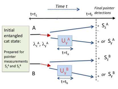
Figure 3: Macroscopic version of the EPR-Bohm paradox: The system is prepared in a cat state, e.g. (15), for which the final outcomes $+$ and $-$ correspond to the macroscopically distinct amplitudes $\alpha$ and $-\alpha$. At each site $A$ and $B$, a switch (dashed arrow) allows the independent and random choice to evolve the systems by $U_{y}$, or not. With no evolution, $S_{z}$ is measured. If the rotation $U_{y}$ takes place, $S_{y}$ is measured. The outcomes for $S_{z}^{A}$ and $S_{z}^{B}$ (and $S_{y}^{A}$ and $S_{y}^{B}$) are anticorrelated.

In order to realise the EPR-Bohm paradox, it is necessary to identify the noncommuting spin observables and the appropriate unitary rotations $U$ at each site required to measure these. For this purpose, we examine the systems $A$ and $B$ as they evolve independently according to local transformations $U_{A}(t_{a})$ and $U_{B}(t_{b})$, defined as

$$U_{A}(t_{a})=e^{-iH_{NL}^{A}t_{a}/\hbar},\ \ U_{B}(t_{b})=e^{-iH_{NL}^{B}t_{b}/\hbar}$$ (16)

where

$$H_{NL}^{A}=\Omega\hat{n}_{a}^{k},\ \ H_{NL}^{B}=\Omega\hat{n}_{b}^{k}.$$ (17)

Here, $t_{a}$ and $t_{b}$ are the times of evolution at each site, $\hat{n}_{a}=\hat{a}^{\dagger}\hat{a}$ and $\hat{n}_{b}=\hat{b}^{\dagger}\hat{b}$, and $\Omega$ is a constant. We consider $k=2$, noting that $k=4$ allows a Bell test manushan-bell-cat-lg . The dynamics of this evolution is well known yurke-stoler-1 ; collapse-revival-bec-2 ; collapse-revival-super-circuit-1 ; wright-walls-gar-1 . If the system $A$ is prepared in a coherent state $|\alpha\rangle$, then after a time $t_{a}=\pi/2\Omega$ the state of the system $A$ becomes manushan-cat-lg ; manushan-bell-cat-lg ; macro-bell-lg ; yurke-stoler-1 ; cat-states-super-cond ; cat-states-mirrahimi

$$U_{\pi/4}^{A}|\alpha\rangle = e^{-i\pi/4}(|\alpha\rangle+i|-\alpha\rangle)/\sqrt{2}.$$ (18)

Here we define $U_{\pi/4}^{A}=U_{A}(\pi/2\Omega)$. A similar transformation $U_{\pi/4}^{B}$ is defined at $B$ for $t_{b}=\pi/2\Omega$. This state is a superposition of two macroscopically distinct states, and is referred to as a cat state after Schrödinger’s paradox s-cat-1935 ; scat-rmp-frowis . Further interaction for the whole period $t_{a}=2\pi/\Omega$ returns the system to the coherent state $|\alpha\rangle$.

The macroscopic version of the EPR-Bohm paradox is depicted in Figure 3. We consider the spin-$1/2$ observables $\hat{S}_{z}=|+\rangle\langle+|-|-\rangle\langle-|$, $\hat{S}_{x}=|+\rangle\langle-|+|-\rangle\langle+|$ and $\hat{S}_{y}=\frac{1}{i}(|+\rangle\langle-|-|-\rangle\langle+|)$, defined for orthogonal states $|\pm\rangle$ of a two-level system, which we also denote by $|\uparrow\rangle_{z}$ and $|\downarrow\rangle_{z}$. Here, we identify the eigenstates $|\pm\rangle$ of $\hat{S}_{z}^{A}$ ($\hat{S}_{z}^{B}$) as the coherent states $|\pm\alpha\rangle$ ($|\pm\beta\rangle$) respectively, with $\alpha$ and $\beta$ real, and in the limit of large $\alpha$ and $\beta$ where orthogonality is justified. In this limit, we define

$$\hat{S}_{z}^{A} = |\alpha\rangle\langle\alpha|-|-\alpha\rangle\langle-\alpha|$$

$$\hat{S}_{x}^{A} = |\alpha\rangle\langle-\alpha|+|-\alpha\rangle\langle\alpha|$$

$$\hat{S}_{y}^{A} = \frac{1}{i}(|\alpha\rangle\langle-\alpha|-|-\alpha\rangle\langle\alpha|)$$ (19)

for system $A$. The scaling corresponds to Pauli spins $\overrightarrow{\sigma}=(\sigma_{x},\sigma_{y},\sigma_{z})$. The spins $\hat{S}_{z}^{B}$, $\hat{S}_{x}^{B}$ and $\hat{S}_{y}^{B}$ for system $B$ are defined in identical fashion on replacing $\alpha$ with $\beta$. We omit operator “hats”, where the meaning is clear.

V.1.2 Performing the measurement of spins $S_{z}$ and $S_{y}$

The EPR-Bohm paradox requires measurement of $S_{z}^{A}$ and $S_{z}^{B}$. The system in the state (15) is prepared for the pointer stage of the measurements of $S_{z}$. This is because for this system, a measurement of (the sign of) $\hat{X}_{A}$ and $\hat{X}_{B}$ is all that is required to complete the $S_{z}^{A}$ and $S_{z}^{B}$ measurement. The local measurement constitutes an optical homodyne, in which the fields are combined with a strong field across a beamsplitter with a relative phase shift $\vartheta$, followed by direct detection in the arms of the beam splitter yurke-stoler-1 . Here, $\vartheta$ is chosen to measure $\hat{X}_{A}$ ($\hat{X}_{B}$), the axis so that $\alpha$ ($\beta$) as real. The $\vartheta$ is defined by the preparation process, usually involving a pump field.

The EPR-Bohm argument also requires measurements of $S_{y}^{A}$ and $S_{y}^{B}$ on the Bell state (15) prepared at time $t_{1}$ (Figure 3). Here, it is required to adjust the measurement-setting by applying a local unitary transformation $U_{y}$ at each site.

The eigenstates of $\hat{S}_{y}$ are often written in the form $|\uparrow\rangle_{y}=(|\uparrow\rangle_{z}+i|\downarrow\rangle_{z})/\sqrt{2}$ and $|\downarrow\rangle_{y}=(|\uparrow\rangle_{z}-i|\downarrow\rangle_{z})/\sqrt{2}$, but the normalization can vary by a phase factor. We can abbreviate as $|\pm\rangle_{y}=\frac{1}{\sqrt{2}}(|\pm\rangle+i|\mp\rangle)$, denoting $|\uparrow\rangle$ as $|+\rangle$, and $|\downarrow\rangle$ as $|-\rangle$, interchangeably. We choose

$$|\uparrow\rangle_{y} = \frac{e^{-i\pi/4}}{\sqrt{2}}(|\uparrow\rangle_{z}+i|\downarrow\rangle_{z})$$

$$|\downarrow\rangle_{y} = \frac{e^{-i\pi/4}}{\sqrt{2}}(|\downarrow\rangle_{z}+i|\uparrow\rangle_{z})=\frac{e^{i\pi/4}}{\sqrt{2}}(|\uparrow\rangle_{z}-i|\downarrow\rangle_{z}),$$

and will denote the eigenstates at different sites by a subscript. We have temporarily dropped for convenience the superscripts and subscripts indicating the $A$ and $B$, since the transformations are local and apply independently to both sites. It is readily verified that the $\hat{S}_{y}|\uparrow\rangle_{y}=|\uparrow\rangle_{y}$ and $\hat{S}_{y}|\downarrow\rangle_{y}=|\downarrow\rangle_{y}$ i.e. $\hat{S}_{y}^{A}|\pm\rangle_{y,A}=\pm|\pm\rangle_{y,A}$ and $\hat{S}_{y}^{B}|\pm\rangle_{y,B}=\pm|\pm\rangle_{y,B}$.

Now we consider how to perform the measurement of $\hat{S}_{y}$. As explained in Section II, the first stage of measurement involves a unitary operation $U_{y}$, giving a transformation to the measurement basis, so that the system is then prepared for the second stage of measurement, which is the “pointer [stage of] measurement” of $\hat{S}_{y}$. The pointer stage constitutes a measurement of the sign $\hat{S}$ of $\hat{X}$, which for large $\alpha$ ($\beta$) will (after $U_{y}$ has been applied) directly yield the outcome $\pm 1$ for the system prepared in $|\pm\rangle_{y}$. To establish $U_{y}$, following the procedure of Eqs. (4-6) and (11-13), any state

$$|\psi\rangle=c_{+}|\uparrow\rangle_{z}+c_{-}|\downarrow\rangle$$ (21)

written in the $z$ basis can be transformed into the $y$ basis, by substituting

$$|\uparrow\rangle_{z} \rightarrow (e^{i\pi/4}|\uparrow\rangle_{y}+e^{-i\pi/4}|\downarrow\rangle_{y})/\sqrt{2}$$

$$|\downarrow\rangle_{z} \rightarrow -i(e^{i\pi/4}|\uparrow\rangle_{y}-e^{-i\pi/4}|\downarrow\rangle_{y})/\sqrt{2},$$ (22)

This gives

$$|\psi\rangle=d_{+}|+\rangle_{y}+d_{-}|-\rangle_{y}$$ (23)

where $d_{\pm}=(c_{\pm}\mp ic_{-})e^{\pm i\pi/4}$. To obtain the transformed state (23), ready for the pointer stage of measurement of $S_{y}$, the system is thus evolved according to

$$U_{y}|\psi_{Bell}\rangle$$ (24)

where $U_{y}\equiv U_{\pi/4}^{-1}=U^{-1}(\pi/2\Omega)$. We explain this result further in the Appendix A for the purpose of clarity.

The $U_{y}$ is the inverse of the transformation $e^{-iH_{NL}t/\hbar}$ where $t=\pi/2\Omega$, given by (18). The $U_{y}$ is achieved by evolving the local system for a time $t=-\pi/2\Omega\equiv 3\pi/2\Omega$, since the solutions are periodic.

Comment

The states $|+\rangle_{y}$ and $|-\rangle_{y}$ refer to the macroscopically distinct coherent states $|\alpha\rangle$ and $|-\alpha\rangle$ defined at the time $t$ after the local unitary rotation $U_{y}$ has taken place. This is important in identifying the macroscopic nature of the paradox. We then see that the premises of weak macroscopic realism defined in Section II.A.2 will apply (Figure 2).

V.1.3 EPR-Bohm argument

The EPR-Bohm argument is as follows (Figure 3). Consider the system prepared in the Bell state (15) at time $t_{1}$ ($\alpha$, $\beta\rightarrow\infty$). One first measures $S_{z}^{A}$ and $S_{z}^{B}$ for this state at time $t_{1}$. The anticorrelation of the Bell state means that the result for $S_{z}^{A}$ at $A$ can be predicted with certainty by the measurement at $B$.

The EPR-Bohm argument continues, by considering measurements of $S_{y}^{A}$ and $S_{y}^{B}$ on the Bell state (15) prepared at time $t_{1}$ (Figure 3). The measurement of $S_{y}^{A}$ ($S_{y}^{B}$) is thus made by applying the local unitary rotation $U_{y}^{A}$ ($U_{y}^{B}$) to the Bell state prepared at $t_{1}$, followed by a measurement of the sign of $X_{A}$ ($X_{B}$). The state of the system prepared after the unitary rotations $U_{y}^{A}$ and $U_{y}^{B}$ is also given as the Bell state (15), which we write as

$$|\psi_{Bell}\rangle_{y,y}=\frac{1}{\sqrt{2}}(|-\rangle_{y}|+\rangle_{y}-|+\rangle_{y}|-\rangle_{y})$$ (25)

where we have taken $\alpha$, $\beta$ large. As with the original paradox given in Section III.A.1, as seen by Eq. (6), the final measurements of $X_{A}$ and $X_{B}$ therefore reveal an anticorrelation between $S_{y}^{A}$ and $S_{y}^{B}$, and the result for $S_{y}^{A}$ can be revealed, with certainty, by measurement of $S_{y}^{B}$ at site $B$. Here, we note the Comment in the above section, that $|\pm\rangle_{y}$ are the macroscopically distinct coherent states $|\alpha\rangle$ and $|-\alpha\rangle$ (or $|\beta\rangle$ and $|-\beta\rangle$) that are realised at the time $t_{f}$ in Figure 3, which corresponds to the time after the transformation $U_{y}$ has been carried out at each location.

The Bohm-EPR argument continues. The correlation between the spins enables an experimentalist at $B$ to determine with certainty either $S_{z}^{A}$ or $S_{y}^{A}$, for the system prepared at $t_{1}$, by choosing the suitable measurement at the site $B$. Assuming EPR’s local realism, this implies that both the spins of system $A$ are predetermined with certainty. Following along the lines of the two-spin paradox of Section III.A.1, this constitutes Bohm’s EPR paradox, because it is not possible to define a local quantum state $\varphi$ for the spin $1/2$ system $A$ at the time $t_{1}$ with simultaneously specified values for both $\hat{S}_{z}^{A}$ and $\hat{S}_{y}^{A}$. The paradox is the inconsistency between macroscopic local realism and the completeness of quantum mechanics.

In the gedanken experiment, it is assumed that the system $A$ is described quantum mechanics as a spin $1/2$ system, which is valid as $\alpha\rightarrow\infty$, where the two coherent states $|\alpha\rangle$ and $|-\alpha\rangle$ are orthogonal. In the same limit, the spin outcomes for $\hat{S}_{z}^{A}$ and $\hat{S}_{z}^{B}$, and also for $\hat{S}_{y}^{A}$ and $\hat{S}_{y}^{B}$, are perfectly anticorrelated, so that this realisation of the EPR-Bohm paradox strictly follows in the macroscopic limit, where $\alpha\rightarrow\infty$. Proposals for finite $\alpha$ that also account for imperfect anticorrelation of the spins are presented in Appendices C and D.

V.2 Two- and three-spin paradox with spins and CNOT gates

A useful realization uses multimode spin states and CNOT gates. This allows a realisation of both types of EPR-Bohm paradox presented in Section III.A, the two- and three-spin versions, at an increasingly macroscopic level depending on the number of modes. Here, because the spin qubits correspond to macroscopically distinct states, the paradoxes will reveal an inconsistency between macroscopic local realism and the completeness of quantum mechanics.

By analogy with the microscopic example of Section III.A.2, the three-spin paradox requires a transformation $U_{x}$ at each site, where (apart from phase factors)

$$U_{x}^{-1}|\uparrow\rangle \rightarrow \frac{1}{\sqrt{2}}(|\uparrow\rangle+|\downarrow\rangle)$$

$$U_{x}^{-1}|\downarrow\rangle \rightarrow \frac{1}{\sqrt{2}}(|\uparrow\rangle-|\downarrow\rangle),$$ (26)

as well as that for $U_{y}$, given as

$$U_{y}^{-1}|\uparrow\rangle_{z} \rightarrow \frac{1}{\sqrt{2}}(|\uparrow\rangle+i|\downarrow\rangle)$$

$$U_{y}^{-1}|\downarrow\rangle_{z} \rightarrow \frac{1}{\sqrt{2}}(|\uparrow\rangle-i|\downarrow\rangle).$$ (27)

The important step is to find a Hamiltonian that gives a realisation of $U_{x}$ and $U_{y}$. In the previous section, for the cat-states involving the coherent states, a transformation $U_{y}$ was specified but not for $U_{x}$. We note that cat-state superpositions $|\alpha\rangle\pm|-\alpha\rangle$ can be created using conditional measurements cat-state-phil ; cat-states-super-cond ; cat-det-map , and open dissipative systems cat-states-wc ; cat-even-odd-transient ; transient-cat-states-leo ; cat-dynamics-ry ; cats-hach ; cat-states-mirrahimi ; cat-det-map ; cat-states-super-cond . However, we prefer to use simple unitary transformations. A realisation based on NOON states is given in Appendix B.

A realisation can be achieved using an array of spins. The qubits of (27) become the macroscopically distinct states $|\uparrow\rangle\equiv|\uparrow\rangle^{\otimes N}$ and $|\downarrow\rangle\equiv|\downarrow\rangle^{\otimes N}$, for large $N$, so that the initial Bell state (4) becomes the two-site GHZ state

$$|\psi_{Bell}\rangle_{z,z}=\frac{1}{\sqrt{2}}(|\uparrow\rangle_{z,A}^{\otimes N}|\uparrow\rangle_{z,B}^{\otimes N}-|\downarrow\rangle_{z,A}^{\otimes N}|\downarrow\rangle_{,B}^{\otimes N}).$$ (28)

The premises of macroscopic realism can be applied to the macroscopically distinct states. Here, $|\uparrow\rangle_{z,J}^{\otimes N}=\prod_{k=1}^{N}|\uparrow\rangle_{J,k}$ where $|\uparrow\rangle_{J,k}$ is the eigenstate of the Pauli spin $\sigma_{z}^{k}$ for the mode labelled $k$ at site $J$, the collection of modes $k=1,..N$ forming the system labelled $J$. The $|\uparrow\rangle_{J}^{\otimes N}$ and $|\downarrow\rangle_{J}^{\otimes N}$ represent macroscopically distinct states, with collective Pauli spin values of $N$ or $-N$, and are eigenstates of the spin product $S_{z}^{J}=\prod_{k=1}^{N}\sigma_{z}^{k}$.

In order to realise the paradox, the transformations $U$ needed at each site $J$ are, for $U_{x}$ and $U_{y}$, of the form (26)-(27), but where we replace $|\uparrow\rangle\equiv|\uparrow\rangle^{\otimes N}$ and $|\downarrow\rangle\equiv|\downarrow\rangle^{\otimes N}$. Generally, one can first consider how to achieve

$$|\uparrow\rangle^{\otimes N}\rightarrow\cos\frac{\theta}{2}|\uparrow\rangle^{\otimes N}+e^{i\vartheta}\sin\frac{\theta}{2}|\downarrow\rangle^{\otimes N}.$$ (29)

Following the experiment described in IBM-macrorealism-1 , the unitary transformations $U_{x}$ and $U_{y}$ are made in two steps.

The first step is a rotation on the single-mode spin $|\uparrow\rangle_{1}\equiv\begin{pmatrix}1\\ 0\end{pmatrix}$, $|\downarrow\rangle_{1}\equiv\begin{pmatrix}0\\ 1\end{pmatrix}$, given by the unitary matrix $U_{\theta,\vartheta}=\begin{pmatrix}\cos\frac{\theta}{2}&-\sin\frac{\theta}{2}\\ e^{i\vartheta}\sin\frac{\theta}{2}&e^{i\vartheta}\cos\frac{\theta}{2}\end{pmatrix}$ where $\vartheta=0$ or $\pi/2$, which transforms the spin as

$$|\uparrow\rangle_{1} \rightarrow U_{\theta,\vartheta}|\uparrow\rangle_{1}=\cos\frac{\theta}{2}|\uparrow\rangle_{1}+e^{i\vartheta}\sin\frac{\theta}{2}|\downarrow\rangle_{1}$$

$$|\downarrow\rangle_{1} \rightarrow U_{\theta,\vartheta}|\downarrow\rangle_{1}=-\sin\frac{\theta}{2}|\uparrow\rangle_{1}+e^{i\vartheta}\cos\frac{\theta}{2}|\downarrow\rangle_{1}.$$ (30)

Here, we drop the subscript $J$ representing the site, for notational simplicity. Choosing $\theta=\pi/2$ gives the starting point for the transformation $U_{x}$ or $U_{y}$ at each site, with $\vartheta=0$ or $\pi/2$ respectively.

A common physical realisation of the spin qubit involves two polarisation modes: $|\uparrow\rangle\equiv|1,0\rangle$ and $|\downarrow\rangle\equiv|0,1\rangle$ defined for two modes $a_{\pm}$ as in Appendix B. The transformation $U_{\theta,\vartheta}$ can then be achieved with a polarizing beam splitter, with mode transformations ($\hat{a}_{\pm}$ are boson operators defining the modes)

$$\hat{c}_{+} = \hat{a}_{+}\cos\theta-\hat{a}_{-}\sin\theta$$

$$e^{i\vartheta}\hat{c}_{-} = \hat{a}_{+}\sin\theta+\hat{a}_{-}\cos\theta.$$ (31)

The $\hat{c}_{\pm}$ are boson operators for the outgoing modes emerging from the beam splitter. The interaction is described by the Hamiltonian $H=i\hbar k(\hat{a}_{+}\hat{a}_{-}^{\dagger}-\hat{a}_{+}^{\dagger}\hat{a}_{-})$ where $\theta=kt$, for $\vartheta=0$. The addition of a $\vartheta=\pi/2$ phase shift (or not) relative to the two outputs gives the mode transformations with the dependence on $\vartheta=0$ or $\pi/2$. If the input is $|\uparrow\rangle$, the output state is

$$|1,0\rangle_{in} = \hat{a}_{+}^{\dagger}|0\rangle$$ (32)

$$= \cos\theta|1,0\rangle_{out}+e^{i\vartheta}\sin\theta|0,1\rangle_{out}.$$

If the input is $|\downarrow\rangle$, the output is found according to

$$|0,1\rangle_{in} = \hat{a}_{-}^{\dagger}|0\rangle$$ (33)

$$= -\sin\theta|1,0\rangle_{out}+e^{i\vartheta}\cos\theta|0,1\rangle_{out}$$

which gives a starting point for the transformation $U_{x}$ (where $\vartheta=0$) and $U_{y}$ (where $\vartheta=\pi/2$) at each site $J$.

The second step of the transformations $U_{x}$ and $U_{y}$ involves a sequence of CNOT gates. Consider the example of two qubits, with the initial state $|00\rangle\equiv|\uparrow\rangle|\uparrow\rangle$. The transformation $U_{\theta,\vartheta}$ on the first qubit evolves the state into:

$$U_{\theta,\vartheta}|\uparrow\rangle|\uparrow\rangle =\cos\frac{\theta}{2}|\uparrow\rangle|\uparrow\rangle+e^{i\vartheta}\sin\frac{\theta}{2}|\downarrow\rangle|\uparrow\rangle.$$ (34)

The subsequent CNOT gate then flips the second (target) qubit to $|1\rangle\equiv|\downarrow\rangle$ if the first (control) qubit is $|1\rangle$. For $n>2$, the CNOT gates will be performed between the first qubit and all other qubits. This gives

$$U_{\theta,\vartheta}|\uparrow\rangle^{\otimes N} =\cos\frac{\theta}{2}|\uparrow\rangle^{\otimes N}+e^{i\vartheta}\sin\frac{\theta}{2}|\downarrow\rangle^{\otimes N}.$$ (35)

In this way, the transformations (26)-(27) for $U_{x}$ and $U_{y}$ can be achieved macroscopically (for large $N$) for each site.

In the two-spin experiment, either $U_{y}$ or $U_{z}$ is selected at each site, in order to measure $S_{y}^{J}$ or $S_{z}^{J}$. We specify that the initial state $|\psi_{Bell}\rangle_{z,z}$ (Eq. (28)) has been prepared for the pointer measurement of $S_{z}^{J}$. This means that a direct detection of the qubit value (such as a direct detection of a photon in the mode $a_{+}$ or $a_{-}$) is all that is required to complete the measurement of $S_{z}^{J}$.

The experiment of IBM-macrorealism-1 used the IBM quantum computer to perform the operations with $N=2-6$, enabling a test of macrorealism. In a macroscopic realisation, similar operations have been performed using Rydberg atoms, for $N\sim 20$ omran-cats .

The analysis given in Section V.A above follows for this example, on replacing the macroscopically distinct states $|\alpha\rangle$ and $|-\alpha\rangle$ with $|\uparrow\rangle^{\otimes N}$ and $|\downarrow\rangle^{\otimes N}$. One can define the macroscopic spins and the eigenstates $|\pm\rangle_{y}$ and $|\pm\rangle_{x}$ of $S_{y}$ and $S_{x}$ similarly. Following the Comment in Section V.A, the states after the transformations $U_{y}$ and $U_{x}$ are thus superpositions of the two macroscopically distinct states $|\uparrow\rangle^{\otimes N}$ and $|\downarrow\rangle^{\otimes N}$ (for large $N$), which are prepared for the pointer measurement. Hence, the premises of weak macroscopic realism defined in Section II.A.2 apply (Figure 2). The application of the premises macroscopic local realism and deterministic macroscopic realism is explained in the next section. The macroscopic paradoxes map onto the microscopic ones discussed in Section III, and the predictions for the correlations follow accordingly.

VI Conclusions from the macroscopic EPR-Bohm paradox

The EPR-Bohm paradoxes of Section V involving cat states give a stronger version of the EPR argument. The predetermined values for the spins are macroscopically distinct, being the amplitudes $\alpha$ and $-\alpha$, or else the collective Pauli spin values of $N$ and $-N$. Two types of EPR paradox based on macroscopic realism can be put forward. The first is based on MLR (or deterministic macroscopic realism), which can be falsified. The second is based on weak macroscopic realism.

VI.1 EPR paradox based on deterministic macroscopic realism

Macroscopic local realism (MLR) is EPR’s local realism when applied to the system of Figure 3, where the outcomes $+$ and $-$ imply macroscopically distinct states for the system defined at time $t_{1}$ (Section II.A.2). The Locality Assertion LR (2) becomes more convincing, since any disturbance of $A$ due to the measurement at $B$ would then require a macroscopic change of the state at $A$. The application of EPR’s local realism to the system for both measurements $S_{z}$ and $S_{y}$ leads to the conclusion that system $A$ is described simultaneously by both hidden variables $\lambda_{z}^{A}$ and $\lambda_{y}^{A}$ at the time $t_{1}$ (and for the three-spin paradox, similarly for $S_{x}$). The macroscopic paradox therefore indicates inconsistency between MLR and the completeness of quantum mechanics. It is important however, that we justify the application of MLR to both measurements.

According to the definition given by Leggett and Garg, the premises of MLR and dMR require identification of two macroscopically distinct states that the system at that time “has available to it”. At the time $t_{1}$, the systems of Section V.A and V.B are superpositions of two states $|\uparrow\rangle_{z}$ and $|\downarrow\rangle_{z}$ ($|\alpha\rangle$ and $|-\alpha\rangle$, or $|\uparrow\rangle^{\otimes N}$ or $|\downarrow\rangle^{\otimes N}$) that can be regarded as macroscopically distinct (for large $\alpha$ and $N$). These states are prepared for the pointer measurement $S_{z}$.

The application of the premises to the set-up also requires that the states $|\uparrow\rangle_{y}$ and $|\downarrow\rangle_{y}$ distinguished by the measurement $\hat{S}_{y}$ be regarded as macroscopically distinct at this time $t_{1}$. The eigenstates can be represented as superpositions e.g. $|\uparrow\rangle_{z}\pm|\downarrow\rangle_{z}$ of the macroscopically distinct states say, $|\alpha\rangle$ and $|-\alpha\rangle$, at this time. It is argued that the superpositions represented by the different probability amplitudes are macroscopically distinct, because two basis states are. The distinction can be made macroscopic in terms of the pointer basis, by applying a unitary transformation $U_{y}$ which does not involve amplification.

The macroscopic versions of the EPR-Bohm paradox can be based on deterministic macroscopic realism alone, defined in Section II.A.2. The term “deterministic” is used, because in the context of the EPR-Bohm setup, the premise implies that the system (at the time $t_{1}$) is simultaneously specified by both hidden variables, $\lambda_{z}^{A}$ and $\lambda_{y}^{A}$. The outcome for measurement of either $S_{z}^{A}$ or $S_{y}^{A}$ at $A$ is considered predetermined, without regard to the measurement apparatus, as in classical mechanics.

We now argue that the assumption of deterministic macroscopic realism (dMR) is equivalent to that of macroscopic local realism (MLR) for the macroscopic EPR set-up. In the EPR set-up, for any macroscopic spin $S_{\theta}^{A}$ ($\theta\equiv z,y$), one may determine which of two macroscopically distinct states the macroscopic system $A$ is in, without disturbing system $A$, by performing a spacelike separated measurement on $B$. Thus, for the Bohm example where we realize anticorrelated outcomes between $A$ and $B$, dMR is implied by MLR. The converse is also true. The premise of dMR is that system $A$ already be in a state with predetermined value $\lambda$ for the spin $S^{A}$ (whether $S_{z}^{A}$ or $S_{y}^{A}$), prior to the measurement being performed. The locality assumption at a macroscopic level is naturally part of the definition of dMR: The value of $\lambda^{A}$ cannot be affected by measurements performed on a spacelike separated system $B$. The anticorrelation allows determination of the predetermined value for $A$, given a measurement at $B$. Thus, it follows that dMR implies MLR. Hence, we use the terms dMR and MLR interchangeably in this paper.

We mention that Leggett and Garg motivated tests of macroscopic realism legggarg-1 . However, in order to establish a test, the additional assumption of noninvasive measurability was introduced for single systems. Therefore, reports of violations of Leggett-Garg inequalities (e.g. asadian-lg ; emary-review ; IBM-macrorealism-1 ; leggett-garg-uola ; NSTmunro-1-1 ; manushan-cat-lg ) do not imply falsification of macroscopic realism, but rather of the combined premises of macrorealism.

The EPR-Bohm paradox for cat states thus illustrates inconsistency between dMR (or MLR) and the notion that quantum mechanics is a complete theory. However, dMR (and MLR) can be falsified by violations of Bell inequalities for cat states manushan-bell-cat-lg ; manushan-cat-lg ; macro-bell-lg ; macro-bell-jeong . We show in Section VII that dMR (and MLR) can also be falsified in a macroscopic GHZ set-up.

VI.2 An EPR paradox based on weak macroscopic realism

It is also possible to make an argument for the incompleteness of quantum mechanics, based on the premise of weak macroscopic realism (wMR) (Figure 4). The macroscopic paradox follows along the same lines as that for weak local realism, given in Section IV, except that the outcomes $+$ and $-$ for the spins $S_{z}$ and $S_{y}$ can be shown to correspond to macroscopically distinct states for the system measured at time $t_{f}$. The EPR-Bohm paradox based on wMR is stronger than that based on deterministic macroscopic realism, or macroscopic local realism, because the assumption of wMR is weaker and is not falsified by the GHZ or Bell predictions.

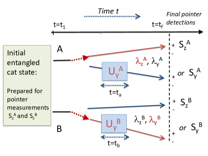
Figure 4: A macroscopic EPR-Bohm paradox based on weak macroscopic realism: The system is as described for Figure 3. At the time $t_{f}$, the sketch depicts the choice to measure $S_{z}^{A}$ and $S_{y}^{B}$. Hence, wMR ascribes to system $A$ at time $t_{f}$ a predetermined value $\lambda_{z}^{A}$ for the outcome for $S_{z}^{A}$, since the system has been prepared for a pointer measurement of $S_{z}^{A}$. The final outcomes for $S_{z}^{A}$ and $S_{z}^{B}$ (and $S_{y}^{A}$ and $S_{y}^{B}$) are anticorrelated. Hence, wMR also ascribes a hidden variable $\lambda_{y}^{A}$ for system $A$ that predetermines the outcome $S_{y}^{A}$.

The argument for the inconsistency between wMR and the notion of the completeness of quantum mechanics is illustrated in Figure 4. At time $t_{f}$ the system $B$ has undergone the evolution $U_{y}^{B}$ to prepare the system $B$ for the pointer measurement of $S_{y}^{B}$, whereas system $A$ is prepared for the pointer measurement of $S_{z}^{A}$. The premise wMR asserts by Assertion (1b) that at time $t_{f}$, a value $\lambda_{z}^{A}$ predetermines the outcome for $S_{z}^{A}$ at $A$, and similarly, a value $\lambda_{y}^{B}$ predetermines the outcome for $S_{y}^{B}$ at $B$. By Assertion (1a), because of the anticorrelation between $A$ and $B$, the value of $\lambda_{y}^{A}=-\lambda_{y}^{B}$ also predetermines the outcome for $S_{y}^{A}$ at $A$, at the time $t_{f}$ (even though a further unitary rotation at $A$ would be necessary to carry out the measurement). Thus, wMR asserts that the system $A$ at the time $t_{f}$ can be simultaneously assigned values $\lambda_{z}^{A}$ and $\lambda_{y}^{A}$ predetermining the results of measurements $S_{z}^{A}$ and $S_{y}^{A}$. Hence, there is an EPR paradox.

The quantum correlations of the macroscopic EPR-Bohm, Bell and GHZ paradoxes are consistent with wMR, because the systems are prepared for a pointer measurement of $S_{z}$ at one time $t_{1}$, and then can be prepared for a pointer measurement of $S_{y}$ at a later time $t_{f}$, after further unitary rotations $U_{A}$ or $U_{B}$. The hidden variables for the EPR-Bohm paradox are tracked in Figure 4. We note wMR does not assert that at the time $t_{f}$, the value of an arbitrary third measurement $S_{\theta}$ is predetermined prior to the unitary rotation, since that rotation $U$ has not been performed at site $A$ or $B$.

For a bipartite system, it is the introduction of a third measurement setting that leads to the falsification of dMR, as evident by the Bell tests which require three or more different measurement settings bell-1969 ; manushan-bell-cat-lg . A falsification is possible for dMR, because the premise dMR asserts that the system $A$ (or $B$) has simultaneously predetermined values for the outcomes of all pointer measurements, at the time $t_{1}$, prior to unitary dynamics $U$ that finalizes the choice of measurement setting.

The ideal experiment realizing the paradox based on wMR would establish that the outcome for $S_{y}^{A}$ can be inferred with certainty from the measurement at $B$. It would also establish that systems $A$ and $B$ are in a superposition (or mixture) of the two relevant macroscopically distinct states. It is also necessary to demonstrate that the system $A$ is a spin $1/2$ system, as in Eqs. (19), e.g. demonstrating both measurements $S_{z}^{A}$ and $S_{y}^{A}$ and the relation (7). Conditions for a realistic experiment are given in Appendix D.

VII GHZ cat gedanken experiment

The GHZ argument outlined in Section III.B becomes macroscopic when the spins $|\uparrow\rangle$ and $|\downarrow\rangle$ correspond to macroscopically distinct states. The macroscopic set-up begins with the preparation at time $t_{1}$ of the GHZ state

$$|\psi_{GHZ}\rangle = \frac{1}{\sqrt{2}}(|\uparrow\rangle_{z,A}|\uparrow\rangle_{z,B}|\uparrow\rangle_{z,C}-|\downarrow\rangle_{z,A}|\downarrow\rangle_{z,B}|\downarrow\rangle_{z,C})$$

where $|\uparrow\rangle_{z,J}\equiv|\uparrow\rangle_{z,J}^{\otimes N}$ and $|\downarrow\rangle_{z,J}\equiv|\downarrow\rangle_{z,J}^{\otimes N}$, defined in Section V.B, are eigenstates of $S_{z}^{J}=\prod_{k=1}^{N}\sigma_{z}^{k}$ with eigenvalues $1$ and $-1$ respectively. Here, $J\equiv A,B,C$ denotes the site. As explained in Section V.B, the system is prepared at $t_{1}$ for a pointer measurement of $S_{z}^{A}S_{z}^{B}S_{z}^{C}$. One then considers the measurements of $S_{x}^{A}S_{x}^{B}S_{x}^{C}$ and $S_{x}^{A}S_{y}^{B}S_{y}^{C}$. By analogy with the microscopic example, this involves applying the transformations $U_{x}$ or $U_{y}$ given by (26)-(27) at each site. After the interactions $U_{x}^{A}$, $U_{x}^{B}$ and $U_{x}^{C}$, the system is prepared for the pointer measurement of $S_{x}^{A}S_{x}^{B}S_{x}^{C}$. The state in the new basis is

$$|\psi_{GHZ}\rangle = \frac{1}{2}(|\downarrow\rangle_{x,A}|\uparrow\rangle_{x,B}|\uparrow\rangle_{x,C}+|\uparrow\rangle_{x,A}|\downarrow\rangle_{x,B}|\uparrow\rangle_{x,C}$$

$$+|\uparrow\rangle_{x,A}|\uparrow\rangle_{x,B}|\downarrow\rangle_{x,C}+|\downarrow\rangle_{x.A}|\downarrow\rangle_{x.B}|\downarrow\rangle_{x,C})$$

The product of the spins is $S_{x}^{A}S_{x}^{B}S_{x}^{C}=-1$.

If we evolve the state (LABEL:eq:ghz-cat) with $U_{x}^{A}$, $U_{y}^{B}$ and $U_{y}^{C}$, the system is prepared for a pointer measurement of $S_{x}^{A}S_{y}^{B}S_{y}^{C}$. In the new basis,

$$|\psi_{GHZ}\rangle = \frac{1}{4}(|\uparrow\rangle_{y,A}|\uparrow\rangle_{y,B}|\uparrow\rangle_{y,C}+|\downarrow\rangle_{y,A}|\downarrow\rangle_{y,B}|\uparrow\rangle_{y,C}$$

$$+|\downarrow\rangle_{y,A}|\uparrow\rangle_{y,B}|\downarrow\rangle_{y,C}+|\uparrow\rangle_{y,A}|\downarrow\rangle_{y,B}|\downarrow\rangle_{y,C}).$$

Always, $S_{x}^{A}S_{y}^{B}S_{y}^{C}=1$. Similarly, we consider $S_{y}^{A}S_{y}^{B}S_{x}^{C}$ and $S_{y}^{A}S_{x}^{B}S_{y}^{C}$, and arrive at the GHZ contradiction, as for the microscopic case. The unitary interactions $U_{x}$ and $U_{y}$ were shown possible using CNOT gates in Section V.B.

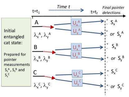
Figure 5: Set-up for the GHZ paradox with cat states. The outcome of $S_{x}$ (and $S_{y}$) at each of the sites $A$, $B$ and $C$ can be predicted with certainty, by choosing certain spacelike separated measurements at the other two sites. EPR’s (macroscopic) local realism implies the outcomes are predetermined by variables $\lambda_{x}$ and $\lambda_{y}$ at the time $t_{1}$, as indicated on the diagram, which gives the GHZ contradiction. The hidden variables can also be deduced from the premise of deterministic macroscopic realism. The GHZ contradiction is a falsification of deterministic macroscopic realism.

VIII Conclusions from the GHZ-cat gedanken experiment

The macroscopic GHZ set-up enables a falsification of the MLR premises, and hence is a stronger version of the GHZ experiment. This is because the states $|\uparrow\rangle_{z,J}\equiv|\uparrow\rangle_{z,J}^{\otimes N}$ and $|\downarrow\rangle_{z,J}\equiv|\downarrow\rangle_{z,J}^{\otimes N}$ are macroscopically distinct for large $N$, and the transformations $U_{x}$ and $U_{y}$ given by (26)-(27) create superpositions of the macroscopically distinct states. Applying the justification given in Section VI.A that the eigenstates $|\uparrow\rangle_{y,J}$ and $|\downarrow\rangle_{y,J}$ (and $|\uparrow\rangle_{x,J}$ and $|\downarrow\rangle_{x,J}$) are also macroscopically distinct, the hidden variables $\lambda_{x}^{A}$, $\lambda_{y}^{A}$, $\lambda_{x}^{B}$, $\lambda_{y}^{B}$, $\lambda_{x}^{C}$, $\lambda_{y}^{C}$ defined for the GHZ system in Section III.B are deduced based on MLR. MLR asserts that the spacelike measurement at $B$ or $C$ cannot induce a macroscopic change to the system $A$. This is a weaker assumption than local realism, which rules out all changes. The GHZ contradiction explained in Section VI.A falsifies MLR.

VIII.1 Falsification of deterministic macroscopic realism

The GHZ paradox as applied to the cat states is also a falsification of deterministic macroscopic realism (dMR). We may present the GHZ paradox directly from the premise of dMR. The premise dMR asserts that the system $A$ (as it exists at time $t_{1}$) can be ascribed a hidden variable $\lambda_{\theta}$, the value of which gives the outcome of the macroscopic spin $S_{\theta}^{A}$, should that measurement be performed, because the eigenstates of $S_{\theta}^{A}$ are assumed macroscopically distinct. The premise dMR asserts that the value of $\lambda_{\theta}$ is not affected by measurements on spacelike separated systems. One may determine which of the two macroscopically distinct states (given by $\lambda_{\theta}=1$ or $-1$) the system $A$ is in, by the measurements on $B$ and $C$. Deterministic macroscopic realism asserts that the hidden variable $\lambda_{\theta}$ applies to the system $A$, prior to the selection of the measurement settings at $B$ and $C$. The set-up is as in Figure 5, where a switch controls whether $S_{x}^{A}$ or $S_{y}^{A}$ will be inferred at $A$, by measuring either $S_{x}^{B}S_{x}^{C}$, or $S_{x}^{B}S_{y}^{C}$. The argument is that the measurement set-up at $B$ and $C$ does not disturb the outcome at $A$, and hence both values, $\lambda_{x}^{A}$ and $\lambda_{y}^{A}$, are simultaneously determined at $A$, at the time $t_{1}$.

The GHZ paradox thus demonstrates that dMR will fail, assuming the paradox can be experimentally realised in agreement with quantum predictions. This is a strong result, giving an “all or nothing” contradiction with dMR. Other macroscopic versions of the GHZ paradox ghz-macro-1 ; ghz-macro-2 ; ghz-macro-3 ; mermin-inequality refer to multidimensional systems, and usually do not address the macroscopic distinction between the spin states. The falsification of MLR and dMR undermines the macroscopic EPR-Bohm argument for the incompleteness of quantum mechanics, given in Section V, which is based on the assumption that these premises are valid.

VIII.2 Consistency of GHZ quantum predictions with wMR and wLR

The conclusion that macroscopic realism does not hold would be a startling one. This motivates consideration of the less restrictive definition of weak macroscopic realism (wMR), defined in Section II.B. The premise wMR can be applied to the GHZ set-up to show there is no inconsistency of wMR with the quantum predictions. This is in agreement with previous work manushan-bell-cat-lg ; delayed-choice-cats , where consistency with wMR was shown for Bell violations using cat states.

To demonstrate the consistency with wMR, we consider state (LABEL:eq:ghz-cat) at time $t_{1}$, and then suppose the systems $B$ and $C$ are prepared so that pointer measurements of $S_{x}^{B}$ and $S_{x}^{C}$, at the time $t_{f}$ will yield the outcomes of $S_{x}^{B}$ and $S_{x}^{C}$ (as in Figure 6). Weak macroscopic realism asserts that the systems are each assigned a predetermined value $\lambda_{x}^{B}$ and $\lambda_{x}^{C}$ respectively for the outcomes of those pointer measurements, at the time $t_{f}$. The premise of wMR also assigns an inferred value

$$\lambda_{x}^{A}\equiv\lambda_{x,inf}^{A}=\lambda_{x}^{B}\lambda_{x}^{C}$$ (39)

to the system $A$, since the values $\lambda_{x}^{B}$ and $\lambda_{x}^{C}$ enable a prediction with certainty for the outcome of the measurement $S_{x}^{A}$, if performed at $A$.

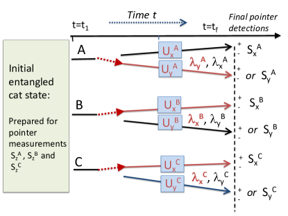
Figure 6: Weak macroscopic realism (wMR) applied to the GHZ experiment. The premise wMR asserts validity of hidden variables for systems at time $t_{f}$ prepared for the pointer measurements. Sketched is the set-up where $S_{y}$ is measured at $A$, and $S_{x}$ at $B$ and $S_{x}$ at $C$. The wMR premise asserts hidden variables for the system $A$ at the time $t_{f}$ that predetermine the final outcome of $S_{y}$ at $A$, and also predetermine the outcome of $S_{x}$ at $A$. This is because the prediction for $S_{x}$ at $A$ can be given with certainty by the pointer measurements at $B$ and $C$. Similar logic implies hidden variables that predetermine the outcomes for both $S_{x}$ and $S_{y}$ for sites $B$ and $C$. However, there is no contradiction with wMR. This is because the hidden variables $\lambda_{x}^{A}$, $\lambda_{y}^{B}$ and $\lambda_{y}^{C}$ give the outcomes of pointer measurements to be made after a further local unitary interaction $U$, assuming there are no further unitary interactions at the other sites.

It is also the case however that wMR applies directly to $A$. If the system $A$ undergoes rotation $U_{y}$, as depicted in Figure 6, then it is prepared in a pointer superposition with respect to $S_{y}^{A}$. Hence the system $A$ is ascribed a hidden variable $\lambda_{y}^{A}$ to predetermine the outcome $S_{y}^{A}$ based on the pointer preparation of the system A itself.

At first glance, this seems to suggest a GHZ contradiction for wMR. Suppose one prepares the systems $B$ and $C$ for the pointer measurements of $S_{x}^{B}$ and $S_{x}^{C}$, at time $t_{f}$ (Figure 6). Hence, for the systems $B$ and $C$ at time $t_{f}$, the outcomes for $S_{x}^{A}$, $S_{x}^{B}$ and $S_{x}^{C}$ are all predetermined, and given by variables $\lambda_{x}^{A}\equiv\lambda_{x,inf}^{A}$, $\lambda_{x}^{B}$ and $\lambda_{x}^{C}$ respectively. Additionally, one can prepare system $A$ in pointer measurement for $y$, and the outcome for $S_{y}^{A}$ is also determined (Figure 6). Then, one can infer the values for the outcomes of measurements $S_{y}^{B}$ and $S_{y}^{C}$, should they be performed by carrying out the appropriate unitary interaction at $B$ and $C$. We have for the inferred values:

$$\lambda_{x,inf}^{A} = -\lambda_{x}^{B}\lambda_{x}^{C}$$

$$\lambda_{y,inf}^{C} = \lambda_{x}^{B}\lambda_{y}^{A}$$

$$\lambda_{y,inf}^{B} = \lambda_{x}^{C}\lambda_{y}^{A}.$$ (40)

For each system, the value of either $S_{x}$ or $S_{y}$ is determined (by the pointer preparation), and the value of the other measurement is determined, by inference of the other (pointer) values. Hence, it appears that there is the GHZ contradiction, because it is as though the outcomes of both $S_{x}$ and $S_{y}$ are determined at each site (at the same time), and these outcomes are either $+1$ or $-1$, hence creating the contradiction of Eq. (14).

However, there is no contradiction with wMR. The value for either $S_{x}$ or $S_{y}$ (the one that is inferred at each site) will require a local unitary rotation $U$ (a change of measurement setting) before the final read-out given by a pointer measurement. The unitary interaction $U$ occurs over a time interval. The unitary rotation means that the value $\lambda$ that predetermines the outcome of the pointer measurement at time $t_{f}$ no longer (necessarily) applies at the later time, $t_{m}$, after the interaction $U$. The system at $t_{m}$ is prepared with respect to a different pointer measurement. Hence, at time $t_{m}$, the earlier predictions of the inferred values $\lambda_{inf}$ for the other sites no longer apply. The paradox as arising from Eq. (14) assumes all values of $\lambda$ apply, to the state at time $t_{f}$.

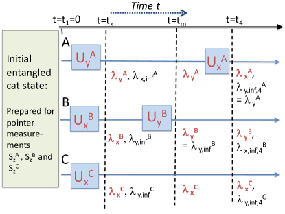
Figure 7: Tracking the hidden variables as given by the premise of weak macroscopic realism (wMR). The dynamics is entirely consistent with the predictions of wMR, despite there being a GHZ paradox. These variables $\lambda$ give the outcomes for the appropriate measurement if performed. The variables in bold red are implied by Assertion (1b) of wMR, that the system is prepared at that time $t_{i}$ at that site, with respect to the pointer basis. The variables indicated by the subscript $inf$ are deduced by Assertion (1a), that the outcome for the measurement can be predicted by the pointer measurements at the other sites, at that time $t_{i}$. The hidden variables that are implied by wMR at the times $t_{i}$ are indicated beside the dashed vertical line labelled $t_{i}$.

In Figure 7, we give more details of the way in which the hidden variables implied by wMR can be tracked and found consistent with the predictions of quantum mechanics. Suppose the system is prepared ready for pointer measurements $S_{y}^{A}$, $S_{x}^{B}$ and $S_{x}^{C}$ at the time $t_{k}$, and the hidden variables $\lambda_{y}^{A}$, $\lambda_{x}^{B}$ and $\lambda_{x}^{C}$ (in bold red) determine those pointer outcomes. The decision is then made to measure instead $S_{y}^{A}$, $S_{y}^{B}$ and $S_{x}^{C}$. This requires a further unitary rotation $\mathbf{U}_{y}^{B}=U_{y}U_{x}^{-1}$ at site $B$. At time $t_{m}$, after $\mathbf{U}_{y}^{B}$ has taken place, the system is described by a different set of hidden variables, $\lambda_{y}^{A}$, $\lambda_{y}^{B}$ and $\lambda_{x}^{C}$. The outcome of the measurement of $S_{y}$ is however determined with certainty by the pointer measurements for $A$ and $C$, as $\lambda_{y}^{B}=\lambda_{y,inf}^{B}=\lambda_{y}^{A}\lambda_{x}^{C}$. At time $t_{m}$, we then see that system $B$ is no longer prepared in a pointer state for $S_{x}$. Hence, at time $t_{m}$, the earlier value of the inferred result $\lambda_{x,inf}^{A}$ at $A$ (which depended on $\lambda_{x}^{B}$) is not relevant. A further unitary rotation $\mathbf{U}_{x}^{A}=U_{x}U_{y}^{-1}$ at $A$ that prepares the system $A$ for a final pointer measurement $S_{x}$ will not (necessarily) give the results that applied at time $t_{k}$ (which was prior to the $U_{y}$ at $B$ taking place). Consider the hidden variables that are defined (based on the premise of wMR) at this time, $t_{4}$, after the evolution $\mathbf{U}_{x}^{A}$. At the time $t_{4}$, the system is ascribed the variables $\lambda_{x}^{A}$, $\lambda_{y}^{B}$ and $\lambda_{x}^{C}$, with $\lambda_{y}^{A}$ also determined, for a future single unitary transformation at $A$. The outcome for $S_{y}$ at $A$ is predetermined (by the pointer outcomes at $B$ and $C$) according to wMR, given by

$$\lambda_{y,inf,4}^{A} = \lambda_{y}^{B}\lambda_{x}^{C}=\lambda_{y,inf}^{B}\lambda_{x}^{C}$$ (41)

$$= \lambda_{x}^{C}\lambda_{y}^{A}\lambda_{x}^{C}$$

$$= \lambda_{y}^{A},$$

which gives consistency with the earlier value at $t_{k}$. However, the outcome for $S_{x}$ at $B$ is inferred from the pointer values at time $t_{4}$:

$$\lambda_{x,inf,4}^{B} = -\lambda_{x}^{A}\lambda_{x}^{C}.$$ (42)

For consistency with the values defined at $t_{k}$, we could propose $\lambda_{x}^{A}=\lambda_{x,inf}^{A}=-\lambda_{x}^{B}\lambda_{x}^{C}$, in which case we would obtain $\lambda_{x,inf,4}^{B}=-\lambda_{x}^{A}\lambda_{x}^{C}=\lambda_{x}^{B}(\lambda_{x}^{C})^{2}=\lambda_{x}^{B}$, giving an apparent consistency with the earlier value. However, the value of $S_{y}$ at $C$ at time $t_{4}$ is inferred to be

$$\lambda_{y,inf,4}^{C} = \lambda_{y}^{B}\lambda_{x}^{A}=\lambda_{y,inf}^{B}\lambda_{x}^{A}$$ (43)

$$= (\lambda_{x}^{C}\lambda_{y}^{A})\lambda_{x}^{A}.$$

Now if we propose $\lambda_{x}^{A}=\lambda_{x,inf}^{A}=-\lambda_{x}^{B}\lambda_{x}^{C}$, we obtain $\lambda_{y,inf,4}^{C}=(\lambda_{x}^{C}\lambda_{y}^{A})(-\lambda_{x}^{B}\lambda_{x}^{C})=-\lambda_{y}^{A}\lambda_{x}^{B}$. We see here that this is different to the earlier value, $\lambda_{y,inf}^{C}=\lambda_{y}^{A}\lambda_{x}^{B}$. Hence, it is not possible to gain consistency between wMR and the values $\lambda$ asserted by the premise of dMR. While dMR is falsified by the GHZ paradox, we see that the GHZ contradiction does not apply to wMR.

We note that according to wMR, the value $\lambda_{y}^{A}$ for system $A$ prepared for the pointer measurement $S_{y}^{A}$, for example, is not changed by unitary rotations that may take place at $B$ or $C$ (Figure 7, at time $t_{m}$). However, if there is a further unitary rotation at $A$, and also at $B$ (i.e. two unitary rotations, at different sites) the value $\lambda_{x,inf}^{A}$ for $S_{x}^{A}$ can change (Figure 7, at time $t_{4}$).

IX Consistency of weak local realism with Bell violations

It has been shown possible to falsify deterministic macroscopic realism for the cat-state system described in Section V.A manushan-bell-cat-lg . This was demonstrated by a violation of Bell inequalities constructed for the macroscopic spins, $|\alpha\rangle$ and $|-\alpha\rangle$. Similarly, in Ref. manushan-bell-cat-lg , it was shown that wMR was not falsified by the Bell violations. This proof was expanded in wigner-friend-macro . Essentially, the same proof holds to show consistency of wLR with Bell violations wigner-friend-macro . For the sake of completeness, we present below the proof demonstrating consistency of wLR with Bell violations. This is relevant, since we note that an identical proof holds to show consistency of wMR with macroscopic Bell violations, where the spins are realised by the macroscopically distinct states $|\uparrow\rangle_{J}\equiv|\uparrow\rangle_{J}^{\otimes N}$ and $|\downarrow\rangle_{z,J}\equiv|\downarrow\rangle_{z,J}^{\otimes N}$ and the unitary operations of the analyzer are realised by the CNOT gates as proposed in Section V.B.

The Bell test involves the EPR-Bohm system. The Pauli spin components defined as

$$\hat{S}_{\theta}^{A} = \hat{S}_{x}^{A}\sin\theta+\hat{S}_{z}^{A}\cos\theta$$

$$\hat{S}_{\phi}^{B} = \hat{S}_{x}^{B}\sin\phi+\hat{S}_{z}^{B}\cos\phi$$ (44)

can be measured by adjusting the analyzer (Stern-Gerlach apparatus or polarizing beam splitter) and the expectation value given by $E(\theta,\phi)=\langle\hat{S}_{\theta}^{A}\hat{S}_{\phi}^{B}\rangle$ measured. According to the EPR-Bohm argument based on EPR’s local realism, each spin component $\hat{S}_{\theta}^{A}$ and $\hat{S}_{\phi}^{B}$ is represented by a hidden variable ($\lambda_{\theta}^{A}$ and $\lambda_{\phi}^{B}$), because the value can be predicted with certainty by a spacelike-separated measurement bell-1971 . This leads to the constraint $-2\leq S\leq 2$ where $S=E(\theta,\phi)-E(\theta,\phi^{\prime})+E(\theta^{\prime},\phi)+E(\theta^{\prime},\phi^{\prime})$, known as the Clauser-Horne-Shimony-Holt-(CHSH) Bell inequality, which is violated for the Bell state (4) bell-1971 ; chsh ; bell-cs-review . The violation therefore falsifies EPR’s premises based on local realism. More generally, the violation shows failure of all local realistic theories defined as those satisfying Bell’s local realism assumptions bell-1971 ; chsh .

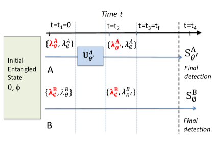
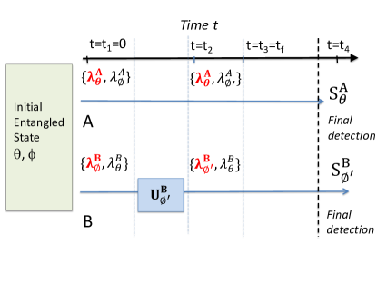
Figure 8: Tracking the hidden variables according to weak local realism (wLR) through the dynamics of the Bell test, which shows violation of the Bell inequality. First, the moment $\langle S_{\theta}^{A}S_{\phi}^{B}\rangle$ is measured. We take the initial time $t_{1}$ to be after the passage through the analysers set at $\theta$ and $\phi$, so that measurement settings $\theta$ and $\phi$ have been determined and the system prepared for the final pointer measurements $S_{\theta}^{A}$ and $S_{\phi}^{B}$. At each time $t_{i}$, wLR implies that certain hidden variables $\lambda$ are valid, depending on the preparation of the system at that time. The hidden variables are depicted in the brackets. Those in red bold are implied by wLR Assertion 1b. Those in black (and not bold) are implied by Assertion 1a.

In the Figure 8, we track the hidden variables that predetermine the values of the spin measurements at each time, based on wLR. We illustrate without loss of generality with one possible time sequence, based on the preparation at the initial time for pointer measurements in the directions $\theta$ and $\phi$. Assuming wLR, the values of $S_{\theta}^{A}$ and $S_{\phi}^{B}$ that are realised by the pointer stage of measurement (if made at that time) are predetermined, given by $\lambda_{\theta}^{A}$ and $\lambda_{\phi}^{B}$ at the time $t_{1}$. Hence

$$E(\theta,\phi)=\langle\lambda_{\theta}^{A}\lambda_{\phi}^{B}\rangle.$$ (45)

To measure $E(\theta^{\prime},\phi)$, there is a further rotation $U_{\theta^{\prime}}^{A}$ at $A$. At time $t_{2}$, the state is prepared for the pointer measurements of $S_{\theta^{\prime}}^{A}$ and $S_{\phi}^{B}$. The hidden variables $\lambda_{\theta^{\prime}}^{A}$ and $\lambda_{\phi}^{B}$ specify the outcomes for those pointer measurements should they be performed. Based on the premise wLR Assertion (1b), these variables are assigned to describe the state of the system at the time $t_{2}$. We note that also because of the anticorrelation evident for spins prepared in the Bell state (4), the wLR Assertion (1a) implies that the hidden variable $\lambda_{\phi}^{B}$ also specifies the outcome of a measurement $S_{\phi}^{A}$, if performed on the system defined at time $t_{2}$. The prediction for wLR is

$$E(\theta^{\prime},\phi)=\langle\lambda_{\theta^{\prime}}^{A}\lambda_{\phi}^{B}\rangle.$$ (46)

Similarly, the measurements of $S_{\theta}^{A}$ and $S_{\phi^{\prime}}^{B}$ require a further rotation $U_{\phi^{\prime}}^{B}$ at $B$, after the initial preparation at $t_{1}$, with no rotation at $A$. A variable $\lambda_{\phi^{\prime}}^{B}$ is defined to give the outcome for $S_{\phi^{\prime}}^{B}$, if that measurement were to be performed at $t_{2}$ after the rotation $U_{\phi^{\prime}}^{B}$. Hence, wLR implies

$$E(\theta,\phi^{\prime})=\langle\lambda_{\theta}^{A}\lambda_{\phi^{\prime}}^{B}\rangle.$$ (47)

Figure 9: Tracking the hidden variables through the dynamics of the Bell test, which shows violation of the Bell inequality. The description is as for Figure 8, but here the moment $\langle S_{\theta^{\prime}}^{A}S_{\phi^{\prime}}^{B}\rangle$ is measured. We note that the conditioning for $\lambda_{\phi^{\prime}}$ necessitates that a rotation $U_{\phi^{\prime}}^{B}$ has also occurred at $B$, as well as $U_{\theta^{\prime}}^{A}$. The nonlocality emerges only after rotations at both sites.

The difference between Bell’s local hidden variable theories and the assertions of wLR are evident when considering measurement of $S_{\theta^{\prime}}^{A}$ and $S_{\phi^{\prime}}^{B}$. This measurement requires two further rotations after the preparation at time $t_{1}$. A possible sequence is given in Figure 9. Suppose the rotation $U_{\theta^{\prime}}^{A}$ is performed first, and at time $t_{2}$, the hidden variables defining the state are $\lambda_{\theta^{\prime}}^{A}$ and $\lambda_{\phi}^{B}$. The pointer measurements are not actually performed, and a rotation $U_{\phi^{\prime}}^{B}$ is then made at $B$. The final state at time $t_{3}$ is given by hidden variables $\lambda_{\theta^{\prime}}^{A}$ and $\lambda_{\phi^{\prime}|\theta^{\prime}}^{B}$. Here, we use subscripts $|\theta^{\prime}$ to specify that $\lambda_{\phi^{\prime}|\theta^{\prime}}^{B}$ is the variable defined for the state specified at the time $t_{3}$, conditioned on the rotation $U_{\theta^{\prime}}^{A}$ at $A$. This is necessary in the context of a wLR model, because the premise of wLR specifies the necessity of locality for the hidden values of the pointer measurements only. The value $\lambda_{\theta^{\prime}}^{A}$ is defined for the pointer measurement of $S_{\theta^{\prime}}^{A}$, and is independent of the choice for $\phi^{\prime}$, since this value $\lambda_{\theta^{\prime}}^{A}$ is (according to wLR) not affected by the unitary rotation $U_{\phi^{\prime}}^{B}$ at the other site $B$. However, we cannot conclude from the wLR assertions that the value of $\lambda_{\phi^{\prime}}^{B}$ defined for the measurement $S_{\phi^{\prime}}^{B}$ on the state after the rotation $U_{\theta^{\prime}}^{A}$ is the same as that defined for pointer measurement $S_{\phi^{\prime}}^{B}$ in Figure 8, where there was no rotation at $A$. Hence we write

$$E(\theta^{\prime},\phi^{\prime})=\langle\lambda_{\theta^{\prime}}^{A}\lambda_{\phi^{\prime}|\theta^{\prime}}^{B}\rangle.$$ (48)

We see that wLR does not imply the CHSH-Bell inequality, which is derived based on the full Bell locality assumption that $\lambda_{\phi^{\prime}}^{B}$ is independent of the value of $\theta^{\prime}$ i.e. is independent of whether the rotation $U_{\theta^{\prime}}^{A}$ has been performed at $A$ or not.

It is well known that the where the values for $\lambda_{\theta}$, $\lambda_{\phi}$, $\lambda_{\theta^{\prime}}$, and $\lambda_{\phi^{\prime}}$ are either $+1$ or $-1$, and if Bell locality is assumed so that $\lambda_{\phi^{\prime}|\theta}^{B}=\lambda_{\phi^{\prime}}^{B}$, then the value of $S$ is bounded by $-2$ and $2$, leading to the CHSH-Bell inequality bell-cs-review . However, where we consider $\lambda_{\phi^{\prime}|\theta}^{B}$ to be an independent variable, $+1$ or $-1$, the bound for $S$ becomes the algebraic bound of $4$. Hence, wLR does not constrain $S$ to be bounded by the Bell inequality.

Nonlocality and deeper models

The wLR and wMR premises allow for nonlocal effects, as evident by the violation of the Bell inequality. This is the meaning of “weak”, that the premises do not encompass the full local realism assumptions of EPR.

The nonlocal effect arises in the above analysis because it cannot be assumed that the value $\lambda_{\phi^{\prime}}^{B}$ is independent of the value $\theta^{\prime}$, which determines the unitary rotation at $A$. The $\lambda_{\theta^{\prime}}^{A}$ is independent of $\phi^{\prime}$, because the setting $\theta^{\prime}$ is fixed (the unitary rotation $U_{\theta^{\prime}}^{A}$ has occurred before $U_{\phi^{\prime}}^{B}$ at $A$), but it cannot be excluded that the $\lambda_{\phi^{\prime}}^{B}$ can depend on $\theta^{\prime}$ because it occurred earlier. It seems to matter which order the unitary rotations are taken, despite that the two rotations occur at spatially separated locations. The predictions will not however depend on the order of rotation. The joint distribution for values $\lambda_{\theta^{\prime}}^{A}$, $\lambda_{\phi^{\prime}}^{B}$ depends on both $\theta^{\prime}$ and $\phi^{\prime}$, the final settings. We note that the conditioning for $\lambda_{\phi^{\prime}}$ necessitates that a rotation $U_{\phi^{\prime}}^{B}$ has also occurred at $B$, since time $t_{1}$. Rotations at both sites are required for the nonlocality to emerge. This feature of wMR and wLR is proved for the GHZ set-up in Section X. We make two comments.

First, the wLR and wMR premises remove the possibility of a strong sort of nonlocality. In these models, the choice to measure $\phi^{\prime}$ instead of $\phi$ at $B$ does not change the value of $\lambda_{\theta}^{A}$ at $A$ once the unitary rotation has occurred at $A$ to fix the measurement setting as $\theta$ at $A$. There is hence no instantaneous nonlocal effect. Similarly, for the system prepared in the Bell state, the value for $S_{\phi}^{A}$ at $A$ is fixed once the rotation $U_{\phi}^{B}$ has occurred at $B$, because the value for $S_{\phi}^{A}$ can be predicted with certainty, even when the unitary rotation $U_{\phi}^{A}$ at $A$ has not occurred. While this gives a nonlocal effect, a further local interaction $U_{\phi}^{A}$ is required at $A$ for the nonlocality to be confirmed.

Second, there is motivation to examine deeper models and tests of quantum mechanics q-contextual-1 ; bohm-hv ; Maroney ; maroney-timpson ; hall-cworlds ; griffiths-histories ; grangier-auffeves-context ; brukner-wigner ; spekkens-toy-model ; q-measurement ; simon-q ; objective-fields-entropy-1 ; castagnoli-2021 ; sabine-retro-toy ; griffiths-nonlocal-not ; roman-schn ; philippe-grang-context-1 ; fr-paradox ; wigner-weak ; bohmian-fr ; losada-wigner-friend for consistency with wLR and wMR. Maroney and Timpson proposed models for macroscopic realism that allow violation of Leggett-Garg inequalities Maroney ; maroney-timpson . In their “supra eigenstate support MR model”, for which there is a predetermination of the outcome of the measurement that distinguishes between two macroscopic distinct states, it is explained that the “state” of the system cannot be an operational eigenstate, meaning it cannot be a preparable state for the system. It is clear from their context that the system is considered to be prepared for a pointer measurement, an example being the observation of a ball in a box. This would give consistency with wMR. The authors gave the de Broglie-Bohm theory as an example of such a model. The de Broglie-Bohm theory is a nonlocal theory for quantum mechanics bohm-hv .

Another model of quantum mechanics that appears consistent with wMR is the objective field theory, motivated by solutions from quantum field theory and the Q function q-contextual-1 ; q-measurement ; simon-q ; objective-fields-entropy-1 . Solutions have been given where the second stage of a measurement is modeled dynamically as amplification of field amplitudes. Here, there is no direct nonlocal mechanism, but rather a retrocausality based on future boundary conditions, which leads to hidden causal loops castagnoli-2021 . The joint distribution for values $\lambda_{\theta^{\prime}}^{A}$, $\lambda_{\phi^{\prime}}^{B}$ is shown to depend on $\theta^{\prime}$ and $\phi^{\prime}$, the final settings, and Bell’s local hidden variable model does not apply. In recent work, it is reported how, for EPR and Bell correlations based on continuous-variable measurements, the premise of wMR is upheld q-measurement . The premise of wMR does not allow retrocausality at a macroscopic level because the hidden variable $\lambda$ is fixed at the given time, being independent of any future event.

X Further predictions for wMR/ wLR

We present further predictions for wMR. These provide a means to experimentally test wMR. The predictions are identical to those of quantum mechanics. However, wMR differs from standard quantum mechanics which does not account for predetermined values of a measurement. The analyses apply in identical fashion to wLR.

X.1 Moments involving a further single rotation are consistent with local realism

Prediction of wMR: We consider the entangled cat-state GHZ system $|\psi\rangle$ (Eq. (LABEL:eq:ghz-cat)) which is then prepared at time $t_{k}$ for pointer measurements $S_{y}^{A}$, $S_{x}^{B}$ and $S_{x}^{C}$ at the respective sites (as in Figure 10). The GHZ contradiction with local realism is realised by first further changing the measurement settings, to measure $S_{x}^{A}$, $S_{x}^{B}$ and $S_{x}^{C}$, which involves one unitary rotation $\mathbf{U}_{x}^{A}$. Also required are measurements $S_{x}^{A}$, $S_{y}^{B}$ and $S_{y}^{C}$, which involve two further rotations, one at each site $B$ and $C$, as well as $\mathbf{U}_{x}^{A}$ (Figure 11). The prediction is that results violating local realism do not arise from the correlations involving only one unitary $U_{x}^{A}$ after the preparation at $t_{k}$. The violations arise from the correlations involving the two further rotations. A similar result was proved for Bell violations manushan-bell-cat-lg .

Proof: We denote the state prepared at the time $t_{k}$ by $|\psi\rangle_{y,x,x}$. A final pointer measurement if conducted at time $t_{k}$ at $A$ gives the outcome for $S_{y}^{A}$. According to wMR, at time $t_{k}$, the values for $S_{x}^{A}$, $S_{y}^{A}$, $S_{x}^{B}$ and $S_{x}^{C}$ are each predetermined, being given by the variables $\lambda_{inf,x}^{A}$, $\lambda_{y}^{A}$, $\lambda_{x}^{B}$ and $\lambda_{x}^{C}$. A single unitary rotation $\mathbf{U}_{x}^{A}=U_{y}^{-1}U_{x}$ at $A$ will enable the result $\lambda_{inf,x}^{A}$ to be revealed. According to wMR, the prediction for $S_{x}^{A}S_{x}^{B}S_{x}^{C}$ is predetermined at time $t_{k}$, for the system prepared in the state $|\psi\rangle_{y,x,x}$. There are hidden variables for each measurement, defined for the system at $t_{k}$. Therefore, if wMR is valid, the prediction for $S_{x}^{A}S_{x}^{B}S_{x}^{C}$, conditioned on the initial state $|\psi\rangle_{y,x,x}$, must be entirely consistent with local realism.$\square$

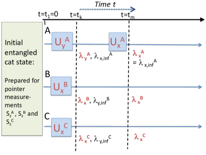
Figure 10: Predictions of weak macroscopic realism (wMR) are consistent with local realism for the single rotation $\mathbf{U_{x}^{A}}$ after preparation at time $t_{k}$. The notation is as for Figure 7. The system at time $t_{k}$ is prepared such that pointer measurements will yield outcomes for measurements of $S_{y}^{A}$, $S_{x}^{B}$ and $S_{x}^{C}$. The prediction for $S_{x}^{A}$ can be inferred from the pointer measurements at $B$ and $C$ and hence is also predetermined at the time $t_{k}$, according to wMR. This measurement requires a further unitary interaction $U_{x}^{A}$. Final pointer measurements at the time $t_{m}$ will yield the result for measurement $S_{x}^{A}S_{x}^{B}S_{x}^{C}$, which by wMR is consistent with local realism. Quantum mechanics also predicts consistency with local realism for the single rotation (see text).

Proof of agreement with quantum prediction: Here, we prove that the prediction of quantum mechanics also shows consistency with local realism for the set-up of just one rotation after preparation (Figure 10). To do this, we compare the predictions of quantum mechanics for the prepared state $|\psi\rangle_{y,x,x}$ against those of a mixed state $\rho_{mix}^{A-BC}$. The state $|\psi\rangle_{y,x,x}$ prepared at time $t_{k}$ in the basis for $S_{y}^{A}$, $S_{x}^{B}$ and $S_{x}^{B}$ is

$$|\psi\rangle_{y,x,x} = \frac{1}{4}\{(|\uparrow\rangle_{y}+|\downarrow\rangle_{y})(|\uparrow\rangle_{x}+|\downarrow\rangle_{x})(|\uparrow\rangle_{x}+|\downarrow\rangle_{x})$$ (49)

$$+i(|\uparrow\rangle_{y}-|\downarrow\rangle_{y})(|\uparrow\rangle_{x}-|\downarrow\rangle_{x})(|\uparrow\rangle_{x}-|\downarrow\rangle_{x})\}$$

$$= \frac{1}{\sqrt{2}}(|\psi_{-}^{A}\rangle|\psi_{+}^{BC}\rangle+|\psi_{+}^{A}\rangle|\psi_{-}^{BC}\rangle)$$

where

$$|\psi_{+}^{BC}\rangle = (|\uparrow\rangle_{x}|\uparrow\rangle_{x}+|\downarrow\rangle_{x}|\downarrow\rangle_{x})/\sqrt{2}$$

$$|\psi_{-}^{BC}\rangle = (|\downarrow\rangle_{x}|\uparrow\rangle_{x}+|\uparrow\rangle_{x}|\downarrow\rangle_{x})/\sqrt{2}$$

and

$$|\psi_{+}^{A}\rangle = \{(1-i)|\uparrow\rangle_{y}+(1+i)|\downarrow\rangle_{y}\}/2$$

$$|\psi_{-}^{A}\rangle = \{(1+i)|\uparrow\rangle_{y}+(1-i)|\downarrow\rangle_{y}\}/2.$$

The state $|\psi\rangle_{y,x,x}$ is a superposition involving entanglement between the system $A$ and the system denoted $BC$, which comprises the systems $B$ and $C$. If the unitary rotation $\mathbf{U}_{x}^{A}$ is performed at $A$, then the prediction for the pointer measurements is $S_{x}^{A}S_{x}^{B}S_{x}^{C}=-1$. Now we compare with the system initially prepared in the mixture

$$\rho_{mix}^{A-BC}=|\psi_{-}^{A}\rangle\langle\psi_{-}^{A}|\rho_{+}^{BC}+|\psi_{+}^{A}\rangle\langle\psi_{+}^{A}|\rho_{-}^{BC}.$$ (50)

Here, $\rho_{+}^{BC}=|\psi_{+}^{BC}\rangle\langle\psi_{+}^{BC}|$ and $\rho_{-}^{BC}=|\psi_{-}^{BC}\rangle\langle\psi_{-}^{BC}|$. This mixture has no entanglement between the system $A$ and the combined systems $B$ and $C$ i.e. it is fully separable with respect to the bipartition that we denote by $A-BC$. If we transform to the $x$ basis at $A$, then we write

$$\rho_{mix}^{A-BC}=|\downarrow\rangle_{x}\langle\downarrow|{}_{x}\rho_{+}^{BC}+|\uparrow\rangle_{x}\langle\uparrow|{}_{x}\rho_{-}^{BC}.$$ (51)

The prediction is $S_{x}^{A}S_{x}^{B}S_{x}^{C}=-1$, which is identical to the prediction for the system prepared in $|\psi\rangle_{y,x,x}$. The quantum prediction for the single unitary interaction $\mathbf{U}_{x}^{A}$ on $|\psi\rangle_{y,x,x}$ is therefore consistent with local realism $-$ since the prediction for $\rho_{mix}^{A-BC}$ is fully local with respect to $A$, arising from a local interaction at $A$.$\square$

The GHZ test showing violation of local realism indeed requires two further rotations, $\mathbf{U}_{y}^{B}$ and $\mathbf{U}_{y}^{C}$ at the sites $B$ and $C$, which allows measurement of $S_{x}^{A}S_{y}^{B}S_{y}^{C}$ (Figure 11). This is because wMR does not (necessarily) predict for the system at time $t_{k}$, a predetermination of the outcomes for both $S_{x}^{A}$ and $S_{y}^{B}$. Hence, there is no contradiction between the predictions of quantum mechanics and wMR. The hidden variables that are predicted by wMR are tracked in the Figure 11. An experiment could be performed, by comparing the observed moments for the GHZ state with those generated by the mixed states.

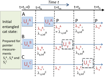
Figure 11: Predictions of weak macroscopic realism (wMR) are consistent with those of quantum mechanics for multiple rotations. The notation is as for Figure 7. Here, further unitary interactions $\mathbf{U}_{y}^{B}$ and $\mathbf{U}_{y}^{C}$ prepare the system for measurement of $S_{x}^{A}S_{y}^{B}S_{y}^{C}$ at the time $t_{5}$. However, at the time $t_{m}$, there is no longer the pointer preparation for $S_{y}^{A}$, and the values that were inferred for measurements $S_{y}^{B}$ and $S_{y}^{C}$ no longer apply. The predictions lead to the GHZ paradox, but are consistent with wMR. The premise wMR also predicts that the results for $S_{x}^{A}S_{y}^{B}S_{y}^{C}$ are independent of when the final irreversible stage of the pointer measurement for $S_{x}^{A}$ is performed, relative to the unitary transformations at $B$ and $C$. The different timings are indicated by the $P$ symbol.

X.2 The timing of the pointer stage of measurement

Prediction of wMR: Consider the system of Figure 11, prepared at time $t_{k}$ so that pointer measurements at $A$, $B$ and $C$ will give the outcomes for $S_{y}^{A}$, $S_{x}^{B}$ and $S_{x}^{C}$. At $A$, the system is then prepared for a pointer measurement of $S_{x}$. At $B$, a unitary rotation then prepares system $B$ for a pointer measurement of $S_{y}^{B}$, and then similarly at $C$. If wMR is valid, then the predictions for the correlations are not dependent on whether the final pointer stages $P$ of the measurement for $S_{x}^{A}$ at $A$ occur before or after the unitary rotations at $B$ and $C$. Here, the final pointer stages of the measurement (denoted $P$ in the Figure) involve a coupling to an environment, whereby the measurement becomes irreversible.

Proof: The premise wMR asserts that the value $\lambda$ for the outcome of the pointer measurement is fixed locally for the appropriately prepared system, provided there is no further unitary $U$ on that system which changes the measurement setting. This prediction agrees with that of quantum mechanics. Quantum calculations do not distinguish the timing of the measurement stage $P$.

XI Conclusion

The main conclusion of this paper is that the negation of local realism, as evidenced by a Bell or GHZ experiment, does not appear to fully resolve the EPR paradox. In summary, we have proposed how EPR-Bohm and GHZ experiments may be realised in mesoscopic and macroscopic regimes, using cat states and suitable unitary interactions. These are significant tests in a setting where all relevant measurements are coarse-grained, distinguishing only between two macroscopically distinct states. The macroscopic EPR-Bohm test illustrates an incompatibility between the assumptions of deterministic macroscopic realism (dMR) and the notion that quantum mechanics is a complete description of physical reality. We explain it is also possible to consider the weaker assumption, weak macroscopic realism (wMR), and to demonstrate a similar inconsistency with the notion that quantum mechanics is a complete theory, using a two-spin version of the EPR-Bohm argument. Yet, while dMR can be falsified by the GHZ experiment, the predictions of the GHZ test agree with those of wMR. Similarly, there is no incompatibility between wMR and violations of macroscopic Bell inequalities. In defining wMR, it is necessary to consider that the measurement occurs in two stages, a reversible stage establishing the measurement setting, and an irreversible stage referred to as the pointer stage of measurement.

Similar conclusions can be drawn for the original EPR and GHZ paradoxes. This paper motivates consideration of a weaker assumption, weak local realism (wLR), in the setting of the original paradox. The EPR argument can be modified to show inconsistency between wLR and the notion that quantum mechanics is a complete description of physical reality. Yet, we show that the predictions of quantum mechanics for the GHZ and Bell experiments are consistent with those of wLR. The definitions of wMR and wLR apply to systems after the choice of measurement basis, and hence do not conflict with the contextuality of quantum mechanics kochen-spekker . Our work may be seen as a supplement to other arguments presented for the incompleteness of quantum mechanics bell-against ; bell-speakable ; s-cat-1935 ; harrigan-spekkens ; delayed-choice-cats ; philippe-grang-context-1 , and may motivate a study of alternative models for quantum mechanics.

In addition to the cat-state experiments, we propose further tests of wLR and wMR. These tests examine correlations after single unitary rotations, and adjust the timing of the unitary interactions that lead to the GHZ contradiction. The predictions of wMR and wLR agree with those of quantum mechanics. The EPR and GHZ paradoxes apply where one can predict with certainty the outcome of a measurement, given measurements at spacelike-separated sites. Experimental factors may prevent the realisation of predictions that are certain. The tests can nonetheless be carried out using inequalities mermin-inequality ; ardehli ; belinski-klyshko ; epr-rmp ; bohm-test-uncertainty ; epr-r2 . Proposals for realistic tests are given in the Appendix.

The proposed experiments could be realised in the microscopic regime using standard techniques where the unitary interactions are performed with polarizing beam splitters. Potential macroscopic realizations are given in Sections V and VII. The two-mode cat states involving coherent states have been generated in cavities cat-det-map ; cat-bell-wang-1 , and GHZ states generated for $N\sim 20$ omran-cats . Mesoscopic realisations of the unitary transformations are in principle feasible using dynamical interactions involving a nonlinear medium, or else CNOT gates.

Appendix

XI.1 The unitary operation $U_{y}$ for measurement of $S_{y}$

Consider the system $A$ originally in the eigenstate for $S_{y}:$

$$|\uparrow\rangle_{y}=\frac{e^{-i\pi/4}}{\sqrt{2}}(|\uparrow\rangle_{z}+i|\downarrow\rangle_{z}),$$ (52)

which is

$$|\uparrow\rangle_{y}\equiv\frac{e^{-i\pi/4}}{\sqrt{2}}(|\alpha\rangle_{z}+i|-\alpha\rangle_{z})$$ (53)

in our realisation. The state after the operation $U_{y}$ is $|\alpha\rangle_{y}$, since we see from (18) that

$$U_{y}|\uparrow\rangle_{y} = U_{\pi/4}^{-1}\frac{e^{-i\pi/4}}{\sqrt{2}}(|\uparrow\rangle_{z}+i|\downarrow\rangle_{z})$$ (54)

$$= |\alpha\rangle$$

The pointer measurement $\hat{S}$ on this state (for large $\alpha$) gives $+1$, corresponding to the outcome required for the eigenstate $|\uparrow\rangle_{y}$. Similarly, consider the system prepared in $|\downarrow\rangle_{y}$

$$|\downarrow\rangle_{y}=\frac{e^{-i\pi/4}}{\sqrt{2}}(|\downarrow\rangle_{z}+i|\uparrow\rangle_{z}$$ (55)

which is

$$|\downarrow\rangle_{y}\equiv\frac{e^{-i\pi/4}}{\sqrt{2}}(|-\alpha\rangle_{z}+i|\alpha\rangle_{z})$$ (56)

The state after the operation $U_{y}$ is $|-\alpha\rangle_{y}$, since from (18), we see that

$$U_{y}|\downarrow\rangle_{y} = |-\alpha\rangle$$ (57)

for which the pointer measurement $X$ gives the outcome $-1$, as required for this eigenstate. Hence, the system that is originally in the linear superposition (23) transforms after $U_{y}$ to

$$U_{y}|\psi\rangle = d_{+}U_{y}|+\rangle_{y}+d_{-}U_{y}|-\rangle_{y}$$ (58)

$$\rightarrow d_{+}|\alpha\rangle+d_{-}|-\alpha\rangle$$

As $\alpha\rightarrow\infty$, the probability of an outcome $+1$ ($-1$) for the measurement $\hat{S}$ of the sign of $\hat{X}_{A}$ is $|d_{+}|^{2}$ ($|d_{-}|^{2}$) respectively, as required.

XI.2 Example of mesoscopic qubits: NOON states

We may also consider where the macroscopic spins are two-mode number states $|N\rangle|0\rangle$ and $|0\rangle|N\rangle$, for $N$ large. We denote two distinct modes by symbols $+$ and $-$, and simplify the notation so that $|N\rangle|0\rangle\equiv|N,0\rangle$ and $|0\rangle|N\rangle\equiv|0,N\rangle$. The macroscopic qubits become $|\uparrow\rangle\rightarrow|N,0\rangle$ and $|\downarrow\rangle\rightarrow|0,N\rangle$. For the GHZ paradoxes, we will consider three sites, labelled $A$, $B$ and $C$. There are two modes (labelled $J+$ and $J-$) identified for each site $J\equiv A$, $B$, $C$. The initial state would be of the form (LABEL:eq:ghz-cat). For each site, we use the transformation macro-bell-lg

$$(U_{y}^{J})^{-1}|N,0\rangle_{J} = e^{i\varphi}(\cos\theta|N,0\rangle_{J}+i\sin\theta|0,N\rangle_{J})$$

$$(U_{y}^{J})^{-1}|0,N\rangle_{J} = ie^{i\varphi}(\sin\theta|N,|0\rangle_{J}-i\cos\theta|0,N\rangle_{J})$$

where $|N,0\rangle_{J}$ and $|N,0\rangle_{J}$ are the two-mode number states at site $J$, and $\varphi$ is a phase-shift. The transformation has been realised to an excellent approximation for $N\lesssim 100$ macro-bell-lg , using the interaction josHam-collett-steel-2-1 ; nonlinear-Ham-1

$$H_{nl}^{J}=\kappa(\hat{a}_{J+}^{\dagger}\hat{a}_{J-}+\hat{a}_{J+}\hat{a}_{J-}^{\dagger})+g\hat{a}_{J+}^{\dagger 2}\hat{a}_{J+}^{2}+g\hat{a}_{J-}^{\dagger 2}\hat{a}_{J-}^{2}$$ (60)

so that $U_{y}^{J}=e^{-iH_{nl}^{J}t/\hbar}$. Here, $\hat{a}_{J+}$, $\hat{a}_{J-}$ are the boson destruction operators for the field modes $J+$ and $J-$, and $\kappa$ and $g$ are the interaction constants. The $\theta$ is a function of the interaction time $t$ and can be selected so that $\theta=\pi/4$. To realize $U_{x}^{J}$ at each site $J\equiv A,B$, $C$, we suppose the field modes $J+$ and $J-$ are spatially separated at the site $J$, so that a phase shift $\theta_{p}$ can be applied along one arm, that of mode $J-$, as used in the detection of NOON states noon-mitchell ; noon-dowling ; noon-afek ; herald-noon-1-2 . For a suitable choice of $\theta_{p}$, this induces an overall relative phase shift between the modes, allowing realisation of the final transformation

$$(U_{x}^{J})^{-1}|N,0\rangle_{J}\rightarrow\cos\theta|N,0\rangle_{J}+\sin\theta|0,N\rangle_{J}.$$ (61)

XI.3 Considerations for a realistic test of the EPR-Bohm paradox

The EPR-Bohm paradox for the two-spin set-up of Section III.A.1 can be signified when

$$(\Delta_{inf}\hat{\sigma}_{y}^{A})^{2}+(\Delta_{inf}\hat{\sigma}_{z}^{A})^{2}<1$$ (62)

where $(\Delta_{inf}\hat{\sigma}_{\theta}^{A})^{2}$ is the variance associated with the estimate inferred for the outcome of $\hat{\sigma}_{\theta}^{A}$ given a result for a measurement of $\hat{\sigma}_{\phi}^{B}$ on system $B$. The value of $\phi$ is chosen optimally to minimize the error epr-r2 ; epr-rmp . Hence, $\phi=\theta$. A sufficient condition that the inequality be satisfied is that

$$(\Delta(\hat{\sigma}_{y}^{A}+\hat{\sigma}_{y}^{B}))^{2}+(\Delta(\hat{\sigma}_{z}^{A}+\hat{\sigma}_{z}^{B}))^{2}<1.$$ (63)

Then the estimate of the outcomes for $\hat{\sigma}_{\theta}^{A}$ is taken to be $-\sigma_{\theta}^{B}$, where $\sigma_{\theta}^{B}$ is the outcome of the measurement $\hat{\sigma}_{\theta}^{B}$, for $\theta=x,y$. The bound of $1$ is half that given by Hofmann and Takeuchi for the entanglement criterion, Eq (24) of their paper hofmann-take , as expected for an EPR-steering inequality epr-steer ; epr-rmp . Clearly, for the EPR-Bohm test given in Sections III and V.B, the inequality is satisfied since there is a perfect anticorrelation between the outcomes, implying the left-side has a value of zero. Similar inequalities can be derived for the three-spin set-up epr-rmp .

For the EPR-Bohm test of Section V.A, the inequality is also satisfied in the limit of $\alpha$ large. However, for finite $\alpha$, the states $|\alpha\rangle$ and $|-\alpha\rangle$ are not truly orthogonal. We propose a realistic experiment as follows. Two orthogonal states $|+\rangle$ and $|-\rangle$ are defined. The spin operators are $\hat{\sigma}_{z}=|+\rangle\langle+|-|-\rangle\langle-|$ and $\hat{\sigma}_{y}=(|+\rangle\langle-|-|-\rangle\langle+|)/i$, where $+$ indicates a state with an outcome for $\hat{X}$ that is non-negative, $x\geq 0$, and $-$ indicates a state with an outcome for $\hat{X}$ that is negative, $x<0$. The notation $x\in+$ implies $x\geq 0$; the notation $x\in-$ implies $x<0$. The state being measured is $|\psi_{Bell}\rangle$, which can be expressed as

$$c_{1}|\alpha\rangle+c_{2}|-\alpha\rangle = c_{+}|+\rangle_{z}+c_{-}|-\rangle_{z}$$ (64)

where

$$|\pm\rangle=\frac{\sum_{x\in\pm}(c_{1}\langle x|\alpha\rangle+c_{2}\langle x|-\alpha\rangle)}{[\sum_{x\in\pm}|c_{1}\langle x|\alpha\rangle+c_{2}\langle x|-\alpha\rangle|^{2}]^{1/2}}|x\rangle$$ (65)

and $c_{\pm}=[\sum_{x\in\pm}|c_{1}\langle x|\alpha\rangle+c_{2}\langle x|-\alpha\rangle|^{2}]^{1/2}$. The measurement of $S_{z}$ corresponds to first determining whether the outcome $x$ of $\hat{X}$ is non-negative or negative.

$$P(\pm) = |c_{\pm}|^{2}=\sum_{x\in\pm}|c_{1}\langle x|\alpha\rangle+c_{2}\langle x|-\alpha\rangle|.^{2}$$ (66)

The overlap function for $\hat{x}=(\hat{a}+\hat{a}^{\dagger})/\sqrt{2}$ where $\alpha$ is real and positive is $\langle x|\alpha\rangle\sim e^{-(x-\sqrt{2}\alpha)^{2}/2}/\pi^{1/4}$ yurke-stoler-1 . Hence,

$$P(+) = \sum_{x\geq 0}|c_{1}\langle x|\alpha\rangle+c_{2}\langle x|-\alpha\rangle|^{2}$$

$$= (\sum_{x\geq 0}|c_{1}|^{2}|\langle x|\alpha\rangle|^{2}+|c_{2}|^{2}|\langle x|-\alpha\rangle|^{2}$$

$$+c_{1}c_{2}^{*}\langle x|\alpha\rangle\langle-\alpha|x\rangle+c_{1}^{*}c_{2}\langle x|-\alpha\rangle\langle\alpha|x\rangle).$$

The leading term is $P(+)=\sum_{x\geq 0}|c_{1}|^{2}|\langle x|\alpha\rangle|^{2}$. The second term is an integral in the tail of the Gaussian, $e^{-(x-\sqrt{2}\alpha)^{2}}/\pi^{1/2}$, which has mean $\mu=\sqrt{2}\alpha$ and standard deviation $\sigma=1/\sqrt{2}$. Taking a conservative value of $\alpha>2$, the probability of the tail is much less than $0.03$. The third and fourth terms are damped by a term of order $e^{-\alpha^{2}}$, and are also negligible for $\alpha>2$. A similar result holds for $P(-)$. The error in assuming $\langle x|-\alpha\rangle=0$ for $x\geq 0$ and $\langle x|\alpha\rangle=0$ for $x<0$ introduces errors of much less than $10$% in the variances of (63). Since the uncertainty bound for the inequality is of order $1$, the errors are negligible for $\alpha>2$.

The measurement of $S_{y}$ requires the rotation

$$U(c_{+}|+\rangle_{z}+c_{-}|-\rangle_{z}) = \frac{1}{\sqrt{2}}(c_{+}-ic_{-})e^{i\pi/4}|+\rangle_{y}$$

$$+\frac{1}{\sqrt{2}}(c_{+}+ic_{-})e^{-i\pi/4}|-\rangle_{y}.$$

so that the probability for an outcome $x\in+$ is

$$|c_{+}-ic_{-}|^{2} = |c_{+}|^{2}+|c_{-}|^{2}$$

$$= \sum_{x\in+}|c_{1}\langle x|\alpha\rangle+c_{2}\langle x|-\alpha\rangle|^{2}$$

$$+\sum_{x\in-}|c_{1}\langle x|\alpha\rangle+c_{2}\langle x|-\alpha\rangle|^{2}.$$

As above, the leading terms are

$$P(+)=\sum_{x\in+}|c_{1}|^{2}|\langle x|\alpha\rangle|^{2}+\sum_{x\in-}|c_{2}|^{2}|\langle x|-\alpha\rangle|^{2},$$ (69)

the remaining terms being negligible for $\alpha>2$. The actual measurement is approximate, being the application of $U$ where:

$$U(c_{1}|\alpha\rangle+c_{2}|-\alpha\rangle) = \frac{c_{1}}{\sqrt{2}}(e^{i\pi/4}|\alpha\rangle+e^{-i\pi/4}|-\alpha\rangle)$$

$$-\frac{ic_{2}}{\sqrt{2}}(e^{i\pi/4}|\alpha\rangle+e^{-i\pi/4}|-\alpha\rangle).$$

This gives

$$\sum_{x\geq 0}\{\frac{(c_{1}-ic_{2})}{\sqrt{2}}e^{i\pi/4}\langle x|\alpha\rangle+\frac{(c_{1}+ic_{2})}{\sqrt{2}}e^{-i\pi/4}\langle x|-\alpha\rangle\}|x\rangle$$

$$+\sum_{x<0}\{\frac{(c_{1}-ic_{2})}{\sqrt{2}}e^{i\pi/4}\langle x|\alpha\rangle+\frac{(c_{1}+ic_{2})}{\sqrt{2}}e^{-i\pi/4}\langle x|-\alpha\rangle\}|x\rangle.$$

Hence,

$$P(+) = \frac{1}{2}\sum_{x\geq 0}|(c_{1}-ic_{2})e^{i\pi/4}\langle x|\alpha\rangle$$ (71)

$$+(c_{1}+ic_{2})e^{-i\pi/4}\langle x|-\alpha\rangle|^{2}.$$

The leading term is given by (69), as required. Any errors in the approximate measurement procedure lead to errors which compared to the uncertainty bound of $1$ are negligible for $\alpha>2$.

XI.4 Considerations for a realistic test of the EPR-Bohm paradox based on weak local realism

The EPR-Bohm paradox based on wLR (or wMR) as described in the set-ups of Figures 2 and 4 can be signified when

$$(\Delta_{inf}\hat{\sigma}_{y}^{A})^{2}+(\Delta_{d}\hat{\sigma}_{z}^{A})^{2}<1.$$ (72)

for measurements on the system prepared at the time $t_{f}$. Here $(\Delta_{inf}\hat{\sigma}_{y}^{A})^{2}$ is the square of the error in the inferred value for $\hat{\sigma_{y}}^{A}$ given the result for the measurement $\hat{\sigma}_{y}^{B}$ on system $B$. The $(\Delta_{d}\hat{\sigma}_{z}^{A})^{2}$ is the square of the error in distinguishing the spin states for the state of system $A$ as prepared at the time $t_{f}$. The inference variance can be measured using standard techniques, as in Appendix C. It is also necessary to confirm that system $A$ is given quantum mechanically as a spin $1/2$ system, which includes defining the two spin eigenstates and demonstrating both spin measurements $\hat{\sigma}_{y}^{A}$ and $\hat{\sigma}_{z}^{A}$ (and their non-commutativity) for the entangled system at time $t_{f}$, as well as confirming the lower bound of the inequality (7). The experiment of Ref. sch-epr-exp-atom reports simultaneous measurement along these lines. There is no violation of the uncertainty principle for the state of system $A$ at time $t_{f}$, because the system $A$ is in one or other spin state with equal probability, implying $(\Delta\hat{\sigma}_{z}^{A})^{2}=1$. In the macroscopic proposals, the pseudo-spin states are the coherent states $|\alpha\rangle$ and $|-\alpha\rangle$, or else $|\uparrow\rangle_{z}\equiv|\uparrow\rangle_{z}^{\otimes N}$ and $|\downarrow\rangle_{z}\equiv|\downarrow\rangle_{z}^{\otimes N}$. Noise can diminish the effectiveness of the measurement $\hat{\sigma}_{z}^{A}$ , increasing $(\Delta_{d}\hat{\sigma}_{z}^{A})^{2}$. The analysis in Appendix C indicates that the error due to the overlap of the coherent states becomes negligible for $\alpha>2$, so that $(\Delta_{d}\hat{\sigma}_{z}^{A})^{2}\rightarrow 0$.

References

- (1) A. Einstein, B. Podolsky, and N. Rosen, Can Quantum-Mechanical Description of Physical Reality Be Considered Complete?, Phys. Rev. 47, 777 (1935).
- (2) J. S. Bell, On the Einstein-Podolsky-Rosen paradox, Physics 1,195 (1964).
- (3) J. F. Clauser, M. A. Horne, A. Shimony and R. A. Holt, Proposed experiment to test local hidden-variable theories, Phys. Rev. Lett. 23, 880 (1969).
- (4) J. S. Bell, Introduction to the hidden-variable question, in: Foundations of Quantum Mechanics ed B d’Espagnat (New York: Academic) pp171-181 (1971).
- (5) J. F. Clauser and A. Shimony, Bell’s theorem: experimental tests and implications, Rep. Prog. Phys. 41, 1881 (1978).
- (6) N. Brunner, D. Cavalcanti, S. Pironio, V. Scarani, and S. Wehner, Bell nonlocality, Rev. Mod. Phys. 86, 419 (2014).
- (7) D. M. Greenberger, M. Home, A. Zeilinger, Going Beyond Bell’s Theorem, in Quantum Theory, and Conceptions of the Universe, M. Kafatos, ed., Kluwer, Dordrecht, The Netherlands (1989), p. 69.
- (8) D. M. Greenberger, M. A. Horne, A. Zeilinger, Bell’s theorem without inequalities, American Journal of Physics 58, 1131(1990).
- (9) N. David Mermin, What’s wrong with these elements of reality? Phys. Today 43 (6), 9 (1990).
- (10) R. K. Clifton, M. L. G. Redhead, J. N. Butterfield, Generalization of the Greenberger-Horne-Zeilinger algebraic proof of nonlocality, Foundations of Physics 21, 149 (1991).
- (11) D. Bouwmeester, J.-W. Pan, M. Daniell, H. Weinfurter, A. Zeilinger, Observation of three-photon Greenberger-Horne-Zeilinger entanglement, Phys. Rev. Lett. 82, 1345 (1999).
- (12) J.-W. Pan, D. Bouwmeester, M. Daniell, H. Weinfurter, A. Zeilinger, Experimental test of quantum nonlocality in three-photon Greenberger–Horne–Zeilinger entanglement, Nature 403, 515 (2000).
- (13) M. D. Reid, P. D. Drummond, W. P. Bowen, E. G. Cavalcanti, P. K. Lam, H. A. Bachor, U. L. Andersen and G. Leuchs, The Einstein-Podolsky-Rosen paradox: From concepts to applications. Rev. Mod. Phys. 81, 1727 (2009).
- (14) E. Schrödinger, Die gegenwärtige Situation in der Quantenmechanik, Die Naturwissenschaften, 23, 807-812; 823-828; 844-849 (1935).
- (15) A. Leggett and A. Garg, Quantum mechanics versus macroscopic realism: is the flux there when nobody looks?, Phys. Rev. Lett. 54, 857 (1985).
- (16) D. Bohm, Quantum Theory (Prentice-Hall, New York, 1951).
- (17) D. Bohm and Y. Aharonov, Discussion of Experimental Proof for the Paradox of Einstein, Rosen and Podolsky, Phys. Rev. 108, 1070 (1957).
- (18) A. Aspect, P. Grangier, G. Roger, Experimental Realization of Einstein-Podolsky-Rosen Bohm Gedankenexperiment: A new violation of Bell’s inequalities. Phys. Rev. Lett. 49, 91 (1982).
- (19) M. Thenabadu and M.D. Reid, Bipartite Leggett-Garg and macroscopic Bell inequality violations using cat states: distinguishing weak and deterministic macroscopic realism, Phys. Rev. A 105, 052207 (2022). M. D. Reid and M Thenabadu, Weak versus deterministic macroscopic realism, arXiv:2101.09476 [quant-ph].
- (20) M. Thenabadu and M. D. Reid, Macroscopic delayed-choice and retrocausality: quantum eraser, Leggett-Garg and dimension witness tests with cat states, Phys. Rev. A 105, 062209 (2022).
- (21) J. S. Bell, On the Problem of Hidden Variables in Quantum Mechanics, Rev. Mod. Phys. 38, 447-52 (1966).
- (22) H. Jeong, M. Paternostro and T. C. Ralph, Failure of Local Realism Revealed by Extremely-Coarse-Grained Measurements, Phys. Rev. Lett. 102, 060403 (2009).
- (23) M. Thenabadu, G-L. Cheng, T. L. H. Pham, L. V. Drummond, L. Rosales-Zárate and M. D. Reid, Testing macroscopic local realism using local nonlinear dynamics and time settings, Phys. Rev. A 102, 022202 (2020).
- (24) R. Rushin Joseph, M. Thenabadu, C. Hatharasinghe, J. Fulton, R-Y Teh, P. D. Drummond and M. D. Reid, Wigner’s Friend paradoxes: consistency with weak-contextual and weak-macroscopic realism models, arXiv 2211.02877 [quant-ph].
- (25) P. Colciaghi, Y. Li, P. Treutlein, and T. Zibold, Einstein-Podolsky-Rosen experiment with two Bose-Einstein condensates, Physical Review X13, 021031 (2023).
- (26) H. Hofmann and S. Takeuchi, Violation of local uncertainty relations as a signature of entanglement, Phys. Rev. A 68, 032103 (2003).
- (27) N. Bohr, Can quantum-mechanical description of physical reality be considered complete?, Phys. Rev. 48, 696 (1935).
- (28) C. Wang et al., A Schrödinger cat living in two boxes, Science 352, 1087 (2016).
- (29) Zaki Leghtas, Gerhard Kirchmair, Brian Vlastakis, Michel H. Devoret, Robert J. Schoelkopf, and Mazyar Mirrahimi, Deterministic protocol for mapping a qubit to coherent state superpositions in a cavity. Phys. Rev. A 87, 042315 (2013).
- (30) B. Yurke and D. Stoler, Generating quantum mechanical superpositions of macroscopically distinguishable states via amplitude dispersion, Phys. Rev. Lett. 57, 13 (1986).
- (31) E. Wright, D. Walls and J. Garrison, Collapses and Revivals of Bose-Einstein Condensates Formed in Small Atomic Samples, Phys. Rev. Lett. 77, 2158 (1996).
- (32) M. Greiner, O. Mandel, T. Hånsch and I. Bloch, Collapse and revival of the matter wave field of a Bose-Einstein condensate, Nature 419, 51 (2002).
- (33) G. Kirchmair et al., Observation of the quantum state collapse and revival due to a single-photon Kerr effect, Nature 495, 205 (2013).
- (34) M. Thenabadu and M. D. Reid, Leggett-Garg tests of macrorealism for dynamical cat states evolving in a nonlinear medium, Phys. Rev. A 99, 032125 (2019).
- (35) B. Vlastakis, G. Kirchmair, Z. Leghtas, S. E. Nigg, L. Frunzio, S. M. Girvin, M. Mirrahimi, M. H. Devoret, R. J. Schoelkopf, Deterministically encoding quantum information using 100-photon schrödinger cat states, Science 342, 607 (2013).
- (36) M. Mirrahimi, Z. Leghtas, V. V. Albert, S. Touzard, R. J. Schoelkopf, L. Jiang, M. H. Devoret, Dynamically protected cat-qubits: a new paradigm for universal quantum computation, New Journal of Physics 16, 045014 (2014).
- (37) F. Frowis, P. Sekatski, W. Dur, N. Gisin, and N. Sangouard, Macroscopic quantum states: measures, fragility, and implementations, Rev. Mod. Phys. 90, 025004 (2018).
- (38) A. Ourjoumtsev, H. Jeong, R. Tualle-Brouri, P. Grangier, Generation of optical ‘Schrödinger cats’ from photon number states, Nature 448,784 (2007).
- (39) M. Wolinsky, H. J. Carmichael, Quantum noise in the parametric oscillator: From squeezed states to coherent-state superpositions, Phys. Rev. Lett. 60 1836 (1988).
- (40) L. Krippner, W. J. Munro, M. D. Reid, Transient macroscopic quantum superposition states in degenerate parametric oscillation: Calculations in the large-quantum-noise limit using the positive p representation, Phys. Rev. A 50, 4330 (1994).
- (41) E. E. Hach III, C. C. Gerry, Generation of mixtures of schrödinger-cat states from a competitive two-photon process, Phys. Rev. A 49, 490 (1994).
- (42) L. Gilles, B. M. Garraway, P. L. Knight, Generation of nonclassical light by dissipative two-photon processes, Phys. Rev. A 49, 2785 (1994).
- (43) R. Y. Teh, F.-X. Sun, R. Polkinghorne, Q. Y. He, Q. Gong, P. D. Drummond, M. D. Reid, Dynamics of transient cat states in degenerate parametric oscillation with and without nonlinear kerr interactions, Phys. Rev. A 101, 043807 (2020).
- (44) H.-Y. Ku, N. Lambert, F.-J. Chan, C. Emary, Y.-N. Chen, F. Nori, Experimental test of non-macrorealistic cat states in the cloud, npj Quantum Information 6, 98 (2020).
- (45) A. Omran, H. Levine, A. Keesling, G. Semeghini, T. T. Wang, S. Ebadi, H. Bernien, A. S. Zibrov, H. Pichler, S. Choi, et al., Generation and manipulation of Schrödinger cat states in Rydberg atom arrays, Science 365, 570 (2019).
- (46) C. Emary, N. Lambert, and F. Nori, Leggett-Garg inequalities, Rep. Prog. Phys 77, 016001 (2014).
- (47) A. Asadian, C. Brukner, and P. Rabl, Probing Macroscopic Realism via Ramsey Correlation Measurements, Phys. Rev. Lett. 112, 190402 (2014).
- (48) G. C. Knee, K. Kakuyanagi, M.-C. Yeh, Y. Matsuzaki, H. Toida, H. Yamaguchi, S. Saito, A. J. Leggett and W. J. Munro, A strict experimental test of macroscopic realism in a superconducting flux qubit, Nat. Commun. 7, 13253 (2016).
- (49) R. Uola, G. Vitagliano and C. Budroni, Leggett-Garg macrorealism and the quantum nondisturbance conditions, Phys. Rev. A 100, 042117 (2019).
- (50) M. D. Reid and W. J. Munro, Macroscopic boson states exhibiting the Greenberger-Horne-Zeilinger contradiction with local realism, Phys. Rev. Lett. 69, 997 (1992).
- (51) Adan Cabello, Multiparty multilevel Greenberger-Horne-Zeilinger states, Phys. Rev. A 63, 022104 (2001).
- (52) W. Son, Jinhyoung Lee, and M. S. Kim, Generic Bell Inequalities for Multipartite Arbitrary Dimensional Systems, Phys. Rev. Lett. 96, 060406 (2006).
- (53) N. D. Mermin, Extreme Quantum Entanglement in a Superposition of Macroscopically Distinct States, Phys. Rev. Lett. 65, 1838 (1990).
- (54) D. Bohm, A suggested interpretation of quantum theory in terms of “hidden” variables”, Phys. Rev. 85, pp 166-179 (1952).
- (55) R. Spekkens, Evidence for the epistemic view of quantum states: A toy theory, Phys Rev A 75, 032110 (2007).
- (56) M. J. Hall, D-A. Deckert, and H. J. Wiseman, Quantum Phenonema modeled by interactions between Many Classical Worlds, Phys. Rev. X4, 041013 (2014).
- (57) A. Auffèves and P. Grangier, Contexts, Systems and Modalities: A new ontology for quantum mechanics, Found. Phys. 46, 121 (2016).
- (58) P. Grangier, Contextual Inferences, Nonlocality, and the Incompleteness of Quantum Mechanics, Entropy 23, 1660 (2021).
- (59) O. J. E. Maroney, Measurements, disturbance and the three-box paradox, Studies in History and Philosophy of Science Part B: Studies in History and Philosophy of Modern Physics, 58, 41 (2017).
- (60) O. J. E. Maroney and C. G. Timpson, Quantum- vs. Macro- Realism: What does the Leggett-Garg Inequality actually test?, arXiv:1412.6139 (2017).
- (61) P. D. Drummond and M. D. Reid, Retrocausal model of reality for quantum fields, Phys. Rev. Research 2, 033266 (2020).
- (62) P. D. Drummond and M. D. Reid, Objective Quantum Fields, Retrocausality and Ontology, Entropy 23, 749 (2021).
- (63) S. Frederich, Introducing the Q-based interpretation of quantum theory, The British Journal for the Philosophy of Science, 0, ja (2021), pp null. arXiv 2106.13502 (2021).
- (64) M. D. Reid and P. D. Drummond, A quantum phase-space equivalence leads to hidden causal loops in a model for measurement consistent with macroscopic realism, arXiv 2205.06070 and arXiv:2303.02373.
- (65) G. Castagnoli, Unobservable causal loops explain both the quantum computational speedup and quantum nonlocality, Phys. Rev. A 104, 032203 (2021).
- (66) R. B. Griffiths, Consistent Quantum Theory (Cambridge University Press, Cambridge, 2002).
- (67) Robert B. Griffiths, Nonlocality claims are inconsistent with Hilbert-space quantum mechanics, Phys. Rev. A 101, 022117 (2020).
- (68) Sandro Donadi and Sabine Hossenfelder, Toy model for local and deterministic wave-function collapse, Phys. Rev. A 106, 022212 (2022).
- (69) R. Schnabel, The solution to the Einstein-Podolsky-Rosen paradox, arXiv:2208.13831.
- (70) C. Brukner, A No-Go Theorem for Observer-Independent Facts, Entropy 20, 350 (2018).
- (71) D. Frauchiger and R. Renner, Quantum theory cannot consistently describe the use of itself, Nat. Commun. 9, 1 (2018).
- (72) M. Losada, R. Laura, and O. Lombardi, Frauchiger-Renner argument and quantum histories, Phys. Rev. A 100, 052114 (2019).
- (73) A. Matzkin and D. Sokolovski, Wigner Friend scenarios with non-invasive weak measurements, Phys. Rev. A 102, 062204 (2020).
- (74) D. Lazarovici and M. Hubert, How Quantum Mechanics can consistently describe the use of itself, Sci. Rep. 9, 470 (2019).
- (75) S. Kochen and E. Specker, The problem of hidden variables in quantum mechanics, Journal of mathematics and mechanics 17, 59 (1967).
- (76) J. Bell, Against measurement, Phys. World 3, 8 pp 33 (1990).
- (77) J. Bell, Speakable and unspeakable in quantum mechanics: Collected papers on quantum philosophy, (Cambridge University Press, 2004).
- (78) N. Harrigan and R. Spekkens, Einstein, incompleteness, and the epistemic view of quantum states, Found. Phys. 40, 125 (2010).
- (79) P. Grangier, Contextual Inferences, Nonlocality, and the Incompleteness of Quantum Mechanics, Entropy 23, 1660 (2021) and references therein.
- (80) E. G. Cavalcanti, P. D. Drummond, H. A. Bachor, and M. D. Reid, Spin entanglement, decoherence and Bohm’s EPR paradox, Optics Express 17 (21), 18693 (2009).
- (81) M. D. Reid, Demonstration of the Einstein-Podolsky-Rosen Paradox using Nondegenerate Parametric Amplification, Phys. Rev. A 40, 913 (1989).
- (82) M. Ardehali, Bell inequalities with a magnitude of violation that grows exponentially with the number of particles, Phys. Rev. A 46, 5375 (1992).
- (83) A. V. Belinskiı, D. N. Klyshko, Interference of light and bell’s theorem, Phys.-Usp. 36, 653 (1993).
- (84) H. J. Lipkin, N. Meshkov, and A. J. Glick, Validity of many-body approximation methods for a solvable model: exact solutions and perturbation theory, Nucl. Phys. 62 188 (1965).
- (85) M. Steel and M. J. Collett, Quantum state of two trapped Bose-Einstein condensates with a Josephson coupling, Phys. Rev. A 57, 2920 (1998).
- (86) M. W. Mitchell, J. S. Lundeen, and A. M. Steinberg, Super-resolving phase measurements with a multiphoton entangled state, Nature 429, 161 (2004).
- (87) I. Afek, O. Ambar, and Y. Silberberg, High-NOON States by Mixing Quantum and Classical Light, Science 328, 879 (2010).
- (88) J. P. Dowling, Quantum optical metrology –the lowdown on high-n00n states, Contemporary Physics 49, 125 (2008).
- (89) S. Slussarenko, M. M. Weston, H. M. Chrzanowski, L. K. Shalm, V. B. Verma, S. W. Nam, G. J. Pryde, Unconditional violation of the shot-noise limit in photonic quantum metrology, Nature Photonics 11, 700 (2017).
- (90) E. G. Cavalcanti, S. J. Jones, H. M. Wiseman, M. D. Reid, Experimental criteria for steering and the Einstein-Podolsky-Rosen paradox, Phys. Rev. A 80, 032112 (2009)