History states of one-dimensional Quantum Walks

Abstract

We analyze the application of the history state formalism to quantum walks. The formalism allows one to describe the whole walk through a pure quantum history state, which can be derived from a timeless eigenvalue equation. It naturally leads to the notion of system-time entanglement of the walk, which can be considered as a measure of the number of orthogonal states visited in the walk. We then focus on one-dimensional discrete quantum walks, where it is shown that such entanglement is independent of the initial spin orientation for real Hadamard-type coin operators and real initial states (in the standard basis) with definite site-parity. Moreover, in the case of an initially localized particle it can be identified with the entanglement of the unitary global operator that generates the whole history state, which is related to its entangling power and can be analytically evaluated. Besides, it is shown that the evolution of the spin subsystem can also be described through a spin history state with an extended clock. A connection between its average entanglement (over all initial states) and that of the operator generating this state is also derived. A quantum circuit for generating the quantum walk history state is provided as well.

I Introduction

Quantum Walks (QW) were first introduced in Aharonov et al. (1993) as a quantum counterpart of classical random walks. While related ideas can be traced back to the works of Feynman on the discretized Dirac equation Feynman et al. (2010), interest on QW has grown enormously in the last decades due to their relevance in the field of quantum computation and information Kempe (2003); Venegas-Andraca (2012). They are useful for the development of quantum algorithms Ambainis (2003), with QW based methods Shenvi et al. (2003); Childs and Goldstone (2004); Berry and Wang (2010) achieving similar speedup to that of the renowned Grover search algorithm Grover (1997). It has also been proven that both continuous and discrete time QW are universal for quantum computation Childs (2009); Lovett et al. (2010). They have been employed in network analysis Sánchez-Burillo et al. (2012) and quantum simulation Lloyd (1996); Berry and Childs (2012); Schreiber et al. (2012); Qiang et al. (2016), as well as for modeling some biological processes Engel et al. (2007); Rebentrost et al. (2009). Besides, QW can be simulated by means of different experimental platforms, such as cold atoms in optical lattices Karski et al. (2009); Preiss et al. (2015); Mugel et al. (2016), trapped ions Schmitz et al. (2009); Zähringer et al. (2010) and photonic setups Gräfe et al. (2016); Flamini et al. (2019); Wang2 et al. (2019); Xu et al. (2019); cardano et al. (2020); QQW et al. (2020); colandrea et al. (2022). Entanglement in QW is also a topic of interest, so far mainly focused on that between coin (spin) and position degrees of freedom Carneiro et al. (2005); Venegas-Andraca et al. (2005); Abal et al. (2006); Omar et al. (2006); Maloyer and Kendon (2007); Annabestani et al. (2010); Romanelli (2010); Ide et al. (2011); Allés et al. (2012); Vieira et al. (2014); Orthey and Amorim (2017); QQW et al. (2020); colandrea et al. (2022).

The aim of this work is to apply the history state formalism Page and Wootters (1983); Rovelli (1990); Isham (1994); Giovannetti et al. (2015); Moreva et al. (2014); McClean and Aspuru-Guzik (2015); Boette et al. (2016); Boette and Rossignoli (2018) to QW. In this formalism, originally proposed by Page and Wootters Page and Wootters (1983), time is incorporated through a reference quantum clock and the system evolution emerges from an entangled system-clock history state which fulfills a timeless Wheeler-DeWitt-like equation DeWitt (1967). The approach has attracted much interest in recent years in different areas, including nonrelativistic quantum mechanics (QM) Giovannetti et al. (2015); Moreva et al. (2014); McClean and Aspuru-Guzik (2015); Boette et al. (2016); Dias and Parisio (2017); Boette and Rossignoli (2018); Nikolova et al. (2018); Coles et al. (2019); Pabón et al. (2019); Cirac et al. (2022) as well as quantum gravity and relativistic QM Rovelli (1990); Isham (1994); Gambini et al. (2009); Zhao et al. (2018); Diaz and Rossignoli (2019); Diaz et al. (2019).

In this work we will focus on one-dimensional discrete QW Ambainis et al. (2001); Konno (2002); Kempe (2003); Venegas-Andraca (2012); Tregenna et al. (2003), in which a spin $1/2$ quantum particle undergoes a unitary evolution in a discrete homogeneous lattice in discrete time steps, according to a translation rule controlled at each step by the value of its spin component and the action of a quantum gate on the spin. We will analyze the walk from the new perspective provided by the history state formalism, here applied in its discrete version McClean and Aspuru-Guzik (2015); Boette et al. (2016); Boette and Rossignoli (2018). The ensuing history state is a pure state of the composite system comprising both the position and spin degrees of freedom on one side (system $S$), and a quantum clock system $T$ on the other. It contains the information of the whole QW and satisfies a timeless eigenvalue equation, such that the state of $S$ at step $n$ can be obtained by conditioning the history state with the corresponding clock state. It can be generated from an initial product state through a quantum circuit.

The corresponding system-time entanglement is a measure of the degree of evolution of $S$, i.e., of the number of orthogonal states visited in the QW, and will be shown to be fully determined by the overlaps between the evolved states. Notice that this entanglement is not the spin-position entanglement usually considered Carneiro et al. (2005); Venegas-Andraca et al. (2005); Abal et al. (2006). We then show that for real Hadamard-type coin operators such entanglement becomes independent of the initial spin state for a wide class of initial position states, including the standard case of an initially localized particle. In the latter, it is also shown that this entanglement is the operator entanglement of the quantum gate generating the history state from the initial product state. Such entanglement defines in fact the entangling power of this operator, which determines the average over all initial spin states of the history state entanglement. In the case of the quadratic entropy it can be evaluated analytically, and an asymptotic expression for large $N$ can be derived in terms of the coin operator parameter, showing explicitly the deviation from the maximum entropy (i.e., maximally entangled) limit. The associated entanglement spectrum is also analyzed.

Besides, it is also possible to define a spin history state by considering a different partition of the whole system, with the spin on one side and a composite clock (the original clock plus the position degree of freedom) on the other. In the case of an initially localized particle the ensuing spin-rest entanglement is shown to be related to that of the unitary operator generating the spin history state. An upper bound to the average spin-rest entanglement is thus obtained, arising from the reduced Schmidt rank of the previous operator.

We first briefly review in Section II the main features of discrete one dimensional QW and their exact evolution. The history state formalism for the QW is introduced in section III, where the main results, together with analytic expressions for overlaps and system–time entanglement entropy are provided. The connection with operator entanglement and the spin history state are discussed in section IV. Illustrative numerical results are shown in both III and IV. Finally conclusions are drawn in V.

II Quantum walks in one dimension

II.1 Generalities

Standard one-dimensional quantum walks are processes in which a quantum “particle” (quantum system) with spin $\frac{1}{2}$ and hence internal Hilbert space $\mathcal{H}_{s}=\mathbb{C}^{2}$, moves along a one-dimensional lattice spanned by position eigenstates $|x\rangle$, $x\in\mathbb{Z}$, which generate the position Hilbert space $\mathcal{H}_{p}$. The full Hilbert space of the system is then $\mathcal{H}_{S}=\mathcal{H}_{p}\otimes\mathcal{H}_{s}$. At each time step two operations are performed such that their composition gives the unitary evolution from one time to the next. The first one acts on the spin component (quantum coin) and leaves the position unchanged. This is usually taken as a kind of generalized Hadamard transform Tregenna et al. (2003), represented in the standard basis (eigenstates $\{|\!\!\uparrow\rangle,|\!\!\downarrow\rangle\}$ of $\sigma_{z}$) as

$$C=\begin{pmatrix}\sqrt{\rho}&\sqrt{1-\rho}\,e^{i\gamma}\\ \sqrt{1-\rho}\,e^{i\phi}&-\sqrt{\rho}\,e^{i(\gamma+\phi)}\end{pmatrix},$$ (1)

where $\gamma,\phi$ are arbitrary angles and $0\leq\rho\leq 1$, such that $C^{\dagger}C=\mathbbm{1}$. We will here focus on traceless real coin operators, such that it results in a Hadamard-type operator

$$C=\begin{pmatrix}\cos\theta&\sin\theta\\ \sin\theta&-\cos\theta\end{pmatrix}=\sigma_{z}\cos\theta+\sigma_{x}\sin\theta\equiv\sigma_{\theta},$$ (2)

with $\sigma_{x}=\begin{pmatrix}0&1\\ 1&0\\ \end{pmatrix}$, $\sigma_{y}=\begin{pmatrix}0&-\imath\\ \imath&0\\ \end{pmatrix}$, $\sigma_{z}=\begin{pmatrix}1&0\\ 0&-1\\ \end{pmatrix}$ the Pauli matrices and $\cos^{2}\theta=\rho$. The usual Hadamard gate is recovered for $\theta=\pi/4$. Any traceless hermitian unitary coin operator $C$ can be written in the form (2) by adequately chosing the $x$ axis.

The second operation is a conditional one-step displacement to the right (left) if spin is up (down) along $z$, generated by the translation operator $T$ ($T^{\dagger}$). The total operator generating the step is then given by

$$U = \tfrac{1}{2}\left[T\otimes(\mathbbm{1}+\sigma_{z})\sigma_{\theta}+T^{\dagger}\otimes(\mathbbm{1}-\sigma_{z})\sigma_{\theta}\right]$$ (3)

$$= \sum_{x}[|x+1\rangle\langle x|\otimes|\!\uparrow\rangle\langle\uparrow\!|\sigma_{\theta}+|x-1\rangle\langle x|\!\downarrow\rangle\langle\downarrow\!|\sigma_{\theta}]\,,\;\;$$ (4)

and verifies the unitary condition $U^{\dagger}U=\mathbbm{1}_{p}\otimes\mathbbm{1}_{s}$.

II.2 Exact evolution and overlaps

Assuming an initial state which is localized in space, i.e., with support in some finite interval, it is convenient, for obtaining a closed exact analytic expression of the evolved states, to consider a finite position basis $\{|x\rangle,x=0,\ldots,M-1\}$, with $\langle x|x^{\prime}\rangle=\delta_{xx^{\prime}}$, which contains the initial state as well as the evolved states up to, say, $N$ steps (i.e. $M>2N$ for an initially localized particle, where $N$ is the number of steps). Then we define the associated discrete Fourier transformed (DFT) basis

$$|k\rangle=\frac{1}{\sqrt{M}}\sum_{x=0}^{M-1}e^{i2\pi xk/M}|x\rangle,\;\;k=0,\ldots,M-1\,,$$ (5)

satisfying $\langle k|k^{\prime}\rangle=\delta_{kk^{\prime}}$ and $|\!-k\rangle=|M\!-\!k\rangle$. These states are the eigenstates of the cyclic translation operator defined by $T|x\rangle=|x+1\rangle$, with $T|M-1\rangle=|0\rangle$, such that

$$T|k\rangle=e^{-i2\pi k/M}|k\rangle\,.$$ (6)

The operator (4) can then be rewritten as

$$U = \exp[-i\frac{2\pi}{M}K\otimes\sigma_{z}](\mathbbm{1}\otimes\sigma_{\theta})$$ (7a)

$$= \begin{pmatrix}e^{-i2\pi K/M}&0\\ 0&e^{i2\pi K/M}\end{pmatrix}\begin{pmatrix}\cos\theta&\sin\theta\\ \sin\theta&-\cos\theta\end{pmatrix}\,,$$ (7b)

where $K$ is the discrete “momentum” operator satisfying $K|k\rangle=k|k\rangle$, such that $T=\exp[-i2\pi K/M]$.

For each value $k$ of $K$, (7b) represents, in the standard spin basis, a unitary operator $U_{k}$ in spin space fulfilling ${\rm Det}[U_{k}]=-1$, with eigenvalues

$$\lambda_{k}^{\pm} = \pm e^{\mp i\omega_{k}}$$ (8a)

$$= \pm\sqrt{1-\cos^{2}\theta\sin^{2}\phi_{k}}-i\cos\theta\sin\phi_{k}\,,$$ (8b)

where $\phi_{k}=2\pi\,k/M$, and eigenvectors

$$|s^{\pm}_{k}\rangle = \alpha^{\pm}_{k}|\!\!\uparrow\rangle+\beta^{\pm}_{k}|\!\!\downarrow\rangle\,,\;\;\frac{\beta^{\pm}_{k}}{\alpha^{\pm}_{k}}=\frac{e^{i\phi_{k}}\lambda_{k}^{\pm}-\cos\theta}{\sin\theta}\,,\;\;\;\;$$ (9)

satisfying $\langle s_{k}^{\nu}|s_{k^{\prime}}^{\nu^{\prime}}\rangle=\delta_{kk^{\prime}}\delta^{\nu\nu^{\prime}}$. Thus,

$$U = \sum_{k=0}^{M-1}|k\rangle\langle k|\otimes U_{k}\,,$$ (10a)

$$U_{k} = e^{-i\omega_{k}}|s_{k}^{+}\rangle\langle s_{k}^{+}|-e^{i\omega_{k}}|s_{k}^{-}\rangle\langle s_{k}^{-}|\,.$$ (10b)

Whereas in the position representation (4) it is the spin which appears as controlling the position displacement, in the momentum representation (10a) based on the eigenbasis of $T$, it is the momentum $K$ which controls the spin evolution at each step.

Using (10) we can now determine the evolution of a general initial product state

$$|\Psi_{0}\rangle =|\psi_{0}\rangle\otimes|\chi_{0}\rangle\,,$$ (11a)

$$|\psi_{0}\rangle =\sum_{x}\psi_{0}(x)|x\rangle=\sum_{k}c_{k}|k\rangle\,,$$ (11b)

$$|\chi_{0}\rangle =\alpha|\!\!\uparrow\rangle+\beta|\!\!\downarrow\rangle\,,$$ (11c)

where $\psi_{0}(x)$ is the initial position state, with

$$c_{k}=\langle k|\psi_{0}\rangle=\frac{1}{\sqrt{M}}\sum_{x}e^{-i2\pi xk/M}\psi_{0}(x)$$ (12)

the DFT of $\psi_{0}(x)$ (sums over $k,x$ are from $0$ to $M-1$) and $\ket{\chi_{0}}$ the initial spin state. The state after $n$ steps is

$$|\Psi_{n}\rangle=U^{n}|\Psi_{0}\rangle=\sum_{k}c_{k}|k\rangle\otimes U^{n}_{k}|\chi_{0}\rangle\,,$$ (13)

where the evolved spin state for momentum $k$ is

$$U_{k}^{n}|\chi_{0}\rangle =e^{-in\omega_{k}}\langle s_{k}^{+}|\chi_{0}\rangle|s_{k}^{+}\rangle+e^{in\omega_{k}}\langle s_{k}^{-}|\chi_{0}\rangle|s_{k}^{-}\rangle\,.$$ (14)

A quantity of most importance in this work is the overlap between the evolved states,

$$\langle\Psi_{n^{\prime}}|\Psi_{n}\rangle = \langle\Psi_{0}|U^{n-n^{\prime}}|\Psi_{0}\rangle=\langle\Psi_{0}|\Psi_{n-n^{\prime}}\rangle$$ (15a)

$$= \sum_{k}|c_{k}|^{2}\langle\chi_{0}|U_{k}^{n-n^{\prime}}|\chi_{0}\rangle$$ (15b)

$$= \sum_{k}|c_{k}|^{2}\!\!\sum_{\nu=\pm 1}\!\!\nu^{n-n^{\prime}}e^{i\nu(n^{\prime}-n)\omega_{k}}|\langle s_{k}^{\nu}|\chi_{0}\rangle|^{2}\,,\;\;\;\;\;\;\;\;$$ (15c)

which depends just on $n-n^{\prime}$.

For future use we notice that for $-k\equiv M-k$, $\lambda_{-k}^{\pm}=\lambda_{k}^{\pm\,*}$ ($\omega_{-k}=-\omega_{k}$) and $|s^{\pm}_{-k}\rangle=|s^{\pm}_{k}\rangle^{*}$ in the standard basis ($\alpha_{-k}^{\pm}=\alpha_{k}^{\pm\,^{*}}$, $\beta_{-k}^{\pm}=\beta_{k}^{\pm\,*}$ in (9)). Moreover,

$$U_{-k}=-\sigma_{y}U_{k}\sigma_{y}\,,$$ (16)

entailing $U_{-k}^{n}=(-1)^{n}\sigma_{y}U_{k}^{n}\sigma_{y}$. It is also evident from (7b) that for $M$ even,

$$U_{k+M/2}=-U_{k}\,.$$ (17)

We finally notice that in the special case $\theta=\pi/2$, $\lambda_{k}^{\pm}=\pm 1$ ($\omega_{k}=0$) and $U_{k}^{2}=\mathbbm{1}_{s}$ $\forall$ $k$, i.e.  $U^{2}=\mathbbm{1}$: the system always returns to its initial configuration after two steps, as $C=\sigma_{x}$ (Eq. (2)) flips the coin at each step.

III Quantum walk history states

III.1 Definition and main properties

Let us now consider a quantum walk with $N-1$ steps, starting from an initial state $|\Psi_{0}\rangle$ at time $t_{0}=0$ and ending in a state $|\Psi_{N-1}\rangle$ at time $t_{N-1}=(N-1)\tau$, where $\tau$ is a certain time scale. We then consider a quantum clock system $T$ with an orthogonal set of states $\ket{n}$, $n=0,\ldots,N-1$, representing the scaled time $n=t_{n}/\tau$ at which the $n^{\rm th}$ step takes place. They are eigenstates of a clock operator $T_{c}$ satisfying $T_{c}|n\rangle=n|n\rangle$, and could represent, for instance, the scaled position of the clock’s needle.

We now define the quantum walk history state as

$$\left|\text{\large$\Psi$}\right\rangle=\frac{1}{\sqrt{N}}\sum_{n=0}^{N-1}|\Psi_{n}\rangle\otimes\ket{n}\,,$$ (18)

where $|\Psi_{n}\rangle$ is the system state (13) at step $n$. The state (18) contains the whole information of the walk. For example, the time average of an observable $O_{S}$ of the particle over the complete walk can be expressed as

$$\langle O_{S}\rangle := \frac{1}{N}\sum_{n=0}^{N-1}\langle\Psi_{n}|O_{S}|\Psi_{n}\rangle$$ (19a)

$$= \langle\text{\large$\Psi$}|O_{S}\otimes\mathbbm{1}_{T}|\text{\large$\Psi$}\rangle\,,$$ (19b)

whereas matrix elements between system states at any two times can be written as

$$\langle\Psi_{n^{\prime}}|O_{S}|\Psi_{n}\rangle =N\langle\text{\large$\Psi$}|(O_{S}\otimes|n^{\prime}\rangle\langle n|)|\text{\large$\Psi$}\rangle\,.$$ (20)

Using Eqs. (13) and (18), the quantum walk history state can be generated from an initial product state $|\psi_{0}\rangle|\chi_{0}\rangle|n=0\rangle$ through the schematic circuit of Fig. 1, where $FT$ implements the transformation $|x\rangle\rightarrow\frac{1}{\sqrt{M}}\sum_{k}e^{-i2\pi xk/M}|k\rangle$. For a particle initially localized at $x=0$, $c_{k}=1/\sqrt{M}$ $\forall$ $k$ and one may replace the FT gate by a simpler Hadamard gate $H^{\otimes m^{\prime}}$, with $2^{m^{\prime}}=M$.

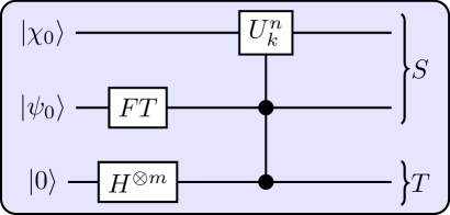
Figure 1: Schematic circuit representing the generation of the history state (18) through Eq. (13): The Quantum Fourier Transform (FT) is applied to the initial position state $|\psi_{0}\rangle$, while $H^{\otimes m}$ denotes the Hadamard operator over $m$ qubits with $2^{m}=N$, such that $H^{\otimes m}|0\rangle=\frac{1}{\sqrt{N}}\sum_{n=0}^{N-1}|n\rangle$. Finally the controlled-$U$ gate $U_{k}^{n}$ acts over the initial spin state $\ket{\chi_{0}}$.

History states actually determine the system evolution when they satisfy a proper timeless eigenvalue equation Boette and Rossignoli (2018). Defining the system-clock unitary operator

$${\cal U}=\sum_{n=1}^{N}U_{n,n-1}\otimes|n\rangle\langle n-1|,$$ (21)

where $U_{n,n-1}=U$ for $1\leq n\leq N-1$ and (identifying $|N\rangle$ with $|0\rangle$) $U_{N,N-1}=(U^{N-1})^{\dagger}$, the state (18) is first seen to be an exact eigenstate of ${\cal U}$ with eigenvalue $1$:

$${\cal U}|\text{\large$\Psi$}\rangle=|\text{\large$\Psi$}\rangle\,.$$ (22)

Conversely, if $|\text{\large$\Psi$}\rangle$ is any state satisfying Eq. (22), i.e. a state which remains fully invariant under ${\cal U}$, then

$$\langle n|\text{\large$\Psi$}\rangle=\langle n|{\cal U}|\text{\large$\Psi$}\rangle=U_{n,n-1}\langle n-1|\text{\large$\Psi$}\rangle\,,$$ (23)

implying that system states $|\Psi_{n}\rangle:=\sqrt{N}\langle n|\text{\large$\Psi$}\rangle$ will fulfill the discrete unitary evolution $|\Psi_{n}\rangle=U_{n,n-1}|\Psi_{n-1}\rangle$, i.e., Eq. (13) for constant $U_{n,n-1}=U$ ($1\leq n\leq N-1$). Normalization $1=\langle\text{\large$\Psi$}|\text{\large$\Psi$}\rangle=\sum_{n}\langle\text{\large$\Psi$}|n\rangle\langle n|\text{\large$\Psi$}\rangle$ then entails $\langle\Psi_{n}|\Psi_{n}\rangle=1$. The whole system evolution up to step $N-1$ is thus determined by Eq. (22) and the initial state $|\Psi_{0}\rangle$. The same holds for general unitaries $U_{n,n-1}$ provided $U_{N,N-1}\ldots U_{1,0}=\mathbbm{1}_{S}$.

Writing ${\cal U}=\exp[-i{\cal J}]$, Eq. (22) implies ${\cal J}|\Psi\rangle=0$ (or $2k\pi$, $k$ integer), which is a discrete Wheeler-DeWitt-type equation DeWitt (1967). In fact, if $U_{n,n-1}=U$ $\forall$ $n=1,\ldots,N$ (such that $U^{N}=\mathbbm{1}$) then ${\cal J}=H\otimes\mathbbm{1}_{T}+\mathbbm{1}_{S}\otimes P_{c}$, where $e^{-iH}=U$ determines the step evolution in $S$ and $e^{-iP_{c}}=\sum_{n=1}^{N}|n\rangle\langle n-1|$ generates the unit translation in the time basis ($|n-1\rangle\rightarrow|n\rangle$) Boette and Rossignoli (2018).

We also mention that the other eigenvalues of ${\cal U}$ are $e^{-i2\pi k/N}$ ($k=0,\ldots,N-1$) Boette et al. (2016); Boette and Rossignoli (2018). Hence, $|\Psi\rangle$ can also be seen as the ground state of the hermitian operator $-\frac{1}{2}({\cal U}+{\cal U^{\dagger}})$, which has eigenvalues $-\cos\frac{2\pi k}{N}$. This enables the use of variational methods for its determination McClean and Aspuru-Guzik (2015); Cirac et al. (2022).

III.2 System-time entanglement

The entanglement $E(S,T)$ of the history state (18) can be regarded as a measure of the “degree of evolution” of system $S$, i.e., of the number of orthogonal states visited in the walk: If $|\Psi_{0}\rangle$ is an eigenstate of $U$, i.e. a stationary state satisfying $U|\Psi_{0}\rangle=e^{i\gamma}|\Psi_{0}\rangle$, the history state becomes separable: $|\text{\large$\Psi$}\rangle=|\Psi_{0}\rangle(\frac{1}{\sqrt{N}}\sum_{n}e^{in\gamma}|n\rangle)$, and $E(S,T)=0$ Boette et al. (2016). This case arises here in finite cyclic realizations when $|\psi_{0}\rangle$ in (14) remains invariant under translations, i.e., when it is a state $|k\rangle$, and $|\chi_{0}\rangle$ coincides with one of the eigenstates $|s_{k}^{\pm}\rangle$ of $U_{k}$, such that $U^{n}|\Psi_{0}\rangle=e^{\mp in\omega_{k}}|\Psi_{0}\rangle$ for $|\Psi_{0}\rangle=|k\rangle\otimes|s_{k}^{\pm}\rangle$.

The opposite situation is an evolution where at each step the system evolves into a new orthogonal state such that $\langle\Psi_{n}|\Psi_{n^{\prime}}\rangle=\delta_{nn^{\prime}}$, in which case $E(S,T)$ is maximum. This evolution arises here in the trivial limit $\theta\rightarrow 0$ for an initially localized state $\psi_{0}(x)=\delta_{xx_{0}}$ with definite spin along the $z$ axis ($\sigma_{z}|\chi_{0}\rangle=\pm|\chi_{0}\rangle$), such that the particle advances always in the same direction.

In the general case $E(S,T)$ will be determined by the overlaps (15). We can expand (18) as ($\nu=\pm 1$)

$$|\text{\large$\Psi$}\rangle =\frac{1}{\sqrt{N}}\sum_{k,\nu,n}\langle k,s_{k}^{\nu}|\Psi_{n}\rangle|k,s_{k}^{\nu}\rangle\otimes|n\rangle$$

$$=\sum_{m=1}^{n_{s}}\sqrt{\lambda_{m}}|m_{S}\rangle\otimes|m_{T}\rangle\,,$$ (24)

where $|k,s_{k}^{\pm}\rangle=|k\rangle\otimes|s_{k}^{\pm}\rangle$ and (24) is its Schmidt representation, obtained from the singular value decomposition (SVD) $M=VDW^{\dagger}$ of the matrix of elements $M_{k\nu,n}=\langle k,s_{k}^{\nu}|\Psi_{n}\rangle/\sqrt{N}$. Here $D_{mm^{\prime}}=\sqrt{\lambda_{m}}\delta_{mm^{\prime}}$ with $\lambda_{m}$ the eigenvalues of the positive semidefinite matrices $MM^{\dagger}$ or equivalently $M^{\dagger}M$ (fulfilling ${\rm Tr}\,M^{\dagger}M=\sum_{m}\lambda_{m}=1$) while $V$, $W$ are unitary matrices diagonalizing $MM^{\dagger}$ and $M^{\dagger}M$ respectively, satisfying $VD=MW$.

In (24) $|m_{S}\rangle=\sum_{k,\nu}V_{k\nu,m}|k,s_{k}^{\nu}\rangle$, $|m_{T}\rangle=\sum_{n}W^{*}_{nm}|n\rangle$ are orthogonal system and clock states respectively ($\langle m_{S(T)}|m^{\prime}_{S(T)}\rangle=\delta_{mm^{\prime}}$) while $n_{s}$ is the Schmidt rank, i.e.  the number of nonzero eigenvalues $\lambda_{m}$, which is just the rank of the matrix $M$. $|\text{\large$\Psi$}\rangle$ is then entangled iff $n_{s}\geq 2$ and separable (product state) if $n_{s}=1$.

Eq. (24) shows that the states $|m_{S(T)}\rangle$ are the eigenvectors of the reduced system and clock states

$$\rho_{S(T)}={\rm Tr}_{T(S)}\,|\text{\large$\Psi$}\rangle\langle\text{\large$\Psi$}|=\sum_{m=1}^{n_{s}}p_{m}|m_{S(T)}\rangle\langle m_{S(T)}|\,,$$ (25)

which determine the average along the walk of any local observable ($\langle\text{\large$\Psi$}|O_{S}\otimes\mathbbm{1}|\text{\large$\Psi$}\rangle\!\!=\!\!{\rm Tr}_{S}\,\rho_{S}O_{S}$), and have the same nonzero eigenvalues $\lambda_{m}$. Their entropies are then identical and define the entanglement entropy of the history state $|\text{\large$\Psi$}\rangle$ (system-time entanglement Boette et al. (2016))

$$E(S,T)=S(\rho_{S})=S(\rho_{T})=\sum_{m}f(\lambda_{m})\,,$$ (26)

where the last expression holds for a general trace-form entropy $S(\rho)={\rm Tr}\,f(\rho)$, where $f$ is a concave nonnegative function satisfying $f(0)=f(1)=0$. Eq. (26) vanishes iff the history state is separable.

The reduced states (25) can be here also written as

$$\rho_{S} = \frac{1}{N}\sum_{n=0}^{N-1}|\Psi_{n}\rangle\langle\Psi_{n}|\,,$$ (27a)

$$\rho_{T} = \frac{1}{N}\sum_{n,n^{\prime}}\langle\Psi_{n^{\prime}}|\Psi_{n}\rangle|n\rangle\langle n^{\prime}|\,.$$ (27b)

Eq.  (27b) shows explicitly that $\rho_{T}$, and hence its eigenvalues $\lambda_{m}$ and the entanglement (26) of the history state, are fully determined by the overlaps (15).

The standard choice for $S$ is the von Neumann entropy

$$S(\rho)=-{\rm Tr}\,\rho\log_{2}\rho,$$ (28)

which will satisfy

$$0\leq E(S,T)\leq\log_{2}N,$$ (29)

such that $2^{E(S,T)}$ is essentially a measure of the number of distinct orthogonal states visited in the evolution. Another convenient choice is the quadratic entropy (also denoted as linear entropy or $q=2$ Tsallis entropy Tsallis (2009)), which is simply determined by the purity ${\rm Tr}\,\rho^{2}$:

$$S_{2}(\rho)=1-{\rm Tr}\,\rho^{2}\,,$$ (30)

and corresponds to $f(\rho)=\rho(\mathbbm{1}-\rho)$. It does not require the explicit determination of eigenvalues and can be measured without requiring a full state tomography Nakazato et al. (2012). It can be here directly evaluated in terms of the overlaps (15): Using (27) together with (26) and (30) we obtain

$$E_{2}(S,T) = 1-\frac{1}{N^{2}}\sum_{n,n^{\prime}}|\langle\Psi_{n^{\prime}}|\Psi_{n}\rangle|^{2}$$ (31a)

$$= 1-\frac{1}{N}[1+2\sum_{n=1}^{N-1}(1-\frac{n}{N})|\langle\Psi_{0}|\Psi_{n}\rangle|^{2}]\,,\;\;\;\;\;\;\;$$ (31b)

where (31b) holds when $|\langle\Psi_{n^{\prime}}|\Psi_{n}\rangle|$ depends just on $|n-n^{\prime}|$, as in Eq. (15) (with factor $\propto 1-\frac{n}{N}$ accounting for the pertinent multiplicity). It obviously satisfies

$$0\leq E_{2}(S,T)\leq 1-\frac{1}{N},$$ (32)

such that $\frac{1}{1-E_{2}(S,T)}$ is here the effective number of orthogonal states visited. A directly related quantity is the $q=2$ Renyi entropy $S_{2}^{R}(\rho)=-\log_{2}(1-S_{2})=-\log_{2}{\rm Tr}\,\rho^{2}$ Beck and Schlögl (1993), which satisfies the same bound (29).

The upper limit in (29)–(32) is reached for $\theta\rightarrow 0$ in (2) and an initially localized particle with definite $\sigma_{z}$. On the other hand, for $\theta=\pi/2$ the evolution becomes periodic with period $2$ (as $U^{2}=\mathbbm{1}$) and hence the system-time entanglement entropy will stay trivially bounded $\forall$ $N$:

$$E(S,T)\leq 1\,,\;\;\;E_{2}(S,T)\leq 1/2\;\;\;(\theta=\pi/2),$$ (33)

with the upper limit reached for an orthogonal intermediate state. Thus, by varying $\theta$ in the interval $[0,\pi/2]$ we can reach, for an initially localized particle, all possible rates of system-time entanglement increase with $N$, from the maximum rate for $\theta=0$ to the null increase for $\theta=\pi/2$, entailing in general a decrease of $E(S,T)$ with increasing $\theta$ in this interval.

III.3 Independence of system-time entanglement from initial spin state

III.3.1 Real initial states with definite site parity

We now examine the entanglement (26) for some general types of initial states $|\Psi_{0}\rangle$. We first notice that if $|\Psi_{0}\rangle$ has a definite position parity, such that its support are just even (or odd) sites $x$,

$$(e^{i\pi X}\otimes\mathbbm{1})|\Psi_{0}\rangle=\pm|\Psi_{0}\rangle,$$ (34)

where $X$ is the discrete position operator $X|x\rangle=x|x\rangle$, the overlap $\langle\Psi_{n}|\Psi_{n^{\prime}}\rangle$ will vanish for $n-n^{\prime}$ odd since at each step the particle will move to sites of opposite parity:

$$(e^{i\pi X}\otimes\mathbbm{1})|\Psi_{n}\rangle=\pm(-1)^{n}|\Psi_{n}\rangle\,.$$ (35)

Eq. (34) is trivially fulfilled for an initially localized particle $\psi_{0}(x)=\delta_{x,x_{0}}$. In momentum space, Eq.  (34) implies $c_{k+M/2}=\pm c_{k}$ ($M$ even) and (35) follows from (17) and (13).

Then, for real $\psi_{0}(x)$ and $\alpha,\beta$ in (11), such that $c_{-k}=c_{k}^{*}$ and $\langle s_{-k}^{\pm}|\chi_{0}\rangle=\langle s_{k}^{\pm}|\chi_{0}\rangle^{*}$, we obtain, using $\sum_{\nu=\pm}|\langle s_{k}^{\nu}|\chi_{0}\rangle|^{2}=1$ and Eq. (15c),

$$\!\!\langle\Psi_{0}|\Psi_{n}\rangle = \sum_{k}|c_{k}|^{2}\cos(n\omega_{k})(|\langle s^{+}_{k}|\chi_{0}\rangle|^{2}+(-1)^{n}|\langle s^{-}_{k}|\chi_{0}\rangle|^{2})$$ (38)

$$= \left\{\begin{array}[]{ccl}\!\!\sum\limits_{k}|c_{k}|^{2}\cos(n\omega_{k})\!\!&,&\!\!n\,{\rm even}\\ 0\!&,&\!\!n\,{\rm odd}\end{array}\right.\!.$$

Thus, the overlap becomes independent of the initial (real) spin state $|\chi_{0}\rangle$ $\forall$ $n$. This implies a system-time entanglement entropy independent of $|\chi_{0}\rangle$.

Previous result can be seen more clearly using Eq. (16) and (15b): since $\sigma_{y}|\chi_{0}\rangle$ is orthogonal to $|\chi_{0}\rangle$ for $|\chi_{0}\rangle$ real ($\alpha,\beta$ real in (11c), equivalent to $\langle\bm{\sigma}\rangle$ in the $x,z$ plane) and $\langle\chi_{0}|U_{-k}^{n}|\chi_{0}\rangle=(-1)^{n}\langle{\chi}_{0}|\sigma_{y}U_{k}^{n}\sigma_{y}|{\chi}_{0}\rangle$, for $|c_{-k}|=|c_{k}|$ and $n$ even we obtain

$$\langle\Psi_{0}|\Psi_{n}\rangle = \frac{1}{2}\sum_{k}|c_{k}|^{2}(\langle\chi_{0}|U_{k}^{n}|\chi_{0}\rangle+\langle{\chi}_{0}|\sigma_{y}U_{k}^{n}\sigma_{y}|\chi_{0}\rangle)$$ (39)

$$= \frac{1}{2}\,\sum_{k}|c_{k}|^{2}\,{\rm Tr}\,U_{k}^{n}={\textstyle\frac{1}{2}}\langle\psi_{0}|{\rm Tr}_{s}\,U^{n}|\psi_{0}\rangle\,,\;\;\;\;\;$$

which shows that the even overlap depends just on the trace of $U_{k}^{n}$, i.e. on the partial trace of $U^{n}$ over spin, and is hence independent of the initial spin state $|\chi_{0}\rangle$. Eq. (39) leads again to (38) for $n$ even and also $n$ odd, as ${\rm Tr}\,U_{k}^{n}=e^{-in\omega_{k}}+(-1)^{n}e^{in\omega_{k}}=(-1)^{n}{\rm Tr}\,U^{n}_{-k}$ and hence the sum in (39) vanishes for $n$ odd when $|c_{-k}|=|c_{k}|$.

With previous expressions, the sum over $N$ in the quadratic system-time entanglement (31b) can be evaluated analytically:

$$\!E_{2}(S,T) = {1-\!\!\!\sum\limits_{\genfrac{}{}{0.0pt}{}{k,k^{\prime}}{\nu=\pm 1}}\!\!\frac{|c_{k}c_{k^{\prime}}|^{2}\sin^{2}\frac{N(\omega_{k}+\nu\omega_{k^{\prime}})}{2}}{N^{2}\sin^{2}(\omega_{k}+\nu\omega_{k^{\prime}})}},\;N\,{\rm even}\;\;$$ (40a)

$$= {1-\!\!\!\!\!\!\!\sum\limits_{\genfrac{}{}{0.0pt}{}{k,k^{\prime}}{\nu,\nu^{\prime}=\pm 1}}\!\!\!\!\!\frac{|c_{k}c_{k^{\prime}}|^{2}\sin^{2}\frac{(N+\nu^{\prime})(\omega_{k}+\nu\omega_{k^{\prime}})}{2}}{2N^{2}\sin^{2}(\omega_{k}+\nu\omega_{k^{\prime}})}},\;N\,{\rm odd}\;\;\;\;\;\;\;\;\;$$ (40b)

Here $\frac{\sin^{2}mu}{m^{2}\sin^{2}u}$ is understood as its limit $1$ if $\sin u=0$ ($m$ integer), being a polynomial of degree $m-1$ in $\cos u$ ($\frac{\sin(n+1)u}{\sin u}=\sum_{k=0}^{\lfloor{n/2}\rfloor}(-1)^{k}\binom{n-k}{k}(2\cos u)^{n-2k}$ is a Chebyshev polynomial of the second kind Abramowitz and Stegun (1965)).

As a check, for $\theta=\pi/2$, $\omega_{k}=0$ $\forall$ $k$ and hence, for any initial $\psi_{0}(x)$ with definite parity, (40a)–(40b) lead to

$$E_{2}(S,T) = \left\{\begin{array}[]{ccl}\frac{1}{2}&,&N\,{\rm even}\\ \frac{1}{2}(1-\frac{1}{N^{2}})&,&N\,{\rm odd}\\ \end{array}\right.\;\;\;(\theta=\pi/2)\,.\;\;$$ (43)

This means that the system just moves between two orthonormal states (periodic evolution) as previously stated, entailing a non-increasing system-time entanglement entropy. The spectrum of $\rho_{S}(T)$ is simply $(\frac{1}{2},\frac{1}{2})$ for $N$ even and $(\frac{N+1}{2N},\frac{N-1}{2N})$ for $N$ odd.

III.3.2 Initially localized particle

For $\psi_{0}(x)=\delta_{xx_{0}}$, $c_{k}=\frac{1}{\sqrt{M}}e^{-i2\pi x_{0}k/M}$ and $|c_{k}|^{2}=\frac{1}{M}$ $\forall\,k$. Overlaps and system-time entanglement are then determined just by the full trace of $U^{n}$ and hence the coin operator angle $\theta$, as implied by (38)-(39):

$$\langle\Psi_{0}|\Psi_{n}\rangle=\frac{{\rm Tr}\,[U^{n}]}{2M}=\left\{\begin{array}[]{cl}\!\!\frac{1}{M}\!\sum_{k}\cos(n\omega_{k}),&n\,{\rm even}\\ 0,&n\,{\rm odd}\end{array}\right..$$ (44)

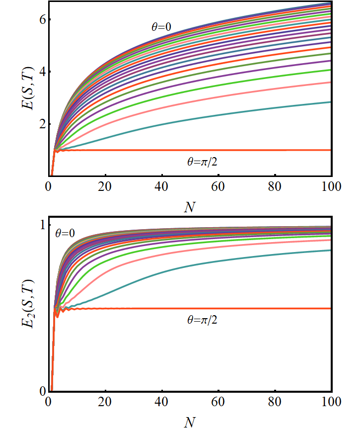
Figure 2: System-time entanglement according to the von Neumann (top) and quadratic (bottom) entropies, as a function of the total number $N$ of steps of the quantum walk for different values $\theta=0,\pi/20.,\ldots,\pi/2$, of the coin operator parameter, for an initially localized particle and any real initial spin state.

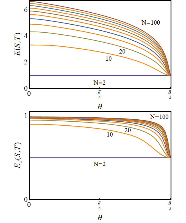
Figure 3: System-time entanglement according to the von Neumann (top) and quadratic (bottom) entropies, as a function of the coin operator angle $\theta$ for different number of steps $N=2,10,20,\ldots,100$, for the same initial states of Fig. 2.

We can now evaluate (44) exactly $\forall$ $\theta$ and $N$, using (8). Since the result is independent of $M$ (for $M>2N$ if $x_{0}=M/2$) it can be obtained either summing over $k$ or letting $M\rightarrow\infty$ and replacing the sum by an integral over $\phi=2\pi k/M$ (with $d\phi=2\pi/M)$. We obtain

$$\langle\Psi_{0}|\Psi_{2n}\rangle = P_{n}(\cos^{2}\theta)\,,$$ (45a)

$$P_{n}(u) = {\textstyle\sum\limits_{j=0}^{n}(-1)^{j}\binom{n}{j}\binom{n+j-1}{j}}u^{j}$$ (45b)

$$= 1-n^{2}u+\tfrac{1}{4}n^{2}(n^{2}-1)u^{2}+\ldots\hskip 14.22636pt$$ (45c)

where $P_{n}(u)=F_{2,1}(-n,n,1,u)=P^{0,-1}_{n}(1-2u)$ is a polynomial of degree $n$ in $u$, with $F_{2,1}$ the hypergeometric function and $P^{\alpha,\beta}_{n}$ the Jacobi polynomial Abramowitz and Stegun (1965). It satisfies $P_{n}(0)=1$ and $P_{n}(1)=0$ $\forall$ $n\geq 1$.

For large $n$ and $\theta\in(0,\pi/2)$, we can also obtain from (45) and the asymptotics of Jacobi polynomials, the exact asymptotic expression

$$\langle\Psi_{0}|\Psi_{2n}\rangle\approx(-1)^{n}\sqrt{\frac{\tan\theta}{n\pi}}\cos(2n\theta+\pi/4)+O(n^{-3/2})\,,$$ (46)

which shows that the overlap fades away as $n^{-1/2}$ for large $n$ and its modulus essentially increases as $\tan^{1/2}\theta$ for increasing $\theta\in(0,\pi/2)$.

Through Eqs. (44)–(45) the quadratic system-time entanglement entropy (31) can be evaluated exactly as:

$$E_{2}^{N}(S,T) = 1-\tfrac{1}{(2MN)^{2}}\sum_{n,n^{\prime}}|{\rm Tr}[U^{n-n^{\prime}}]|^{2}$$ (47a)

$$= {\textstyle 1-\frac{1}{N}[1+2\!\!\!\sum\limits_{n=1}^{\lfloor\frac{N-1}{2}\rfloor}\!\!(1-\frac{2n}{N})P^{2}_{n}(\cos^{2}\theta)].}\;\;\;\;\;\;$$ (47b)

As a check, it is verified that for $\theta=0$, we obtain from (47b) maximum entropy $\forall$ $N$ ($P_{n}(1)=0$ for $n\geq 1$):

$$E_{2}(S,T)=1-\frac{1}{N},\;\;\;\;(\theta=0)\,,$$ (48)

in agreement with previous considerations (any entropy is obviously also maximum in this case). And for $\theta=\pi/2$, we recover from (47b) Eq. (43) for both $N$ even or odd, as $P_{n}(0)=1$ $\forall$ $n\geq 1$. Exact results as a function of $N$ and $\theta$ are depicted in Figs. 2–3.

For large $N$, we may use Eq. (46) for $n\neq 0$ and approximate the sum over $n$ in (47b) by an integral over $u=2n/N$, which leads to the asymptotic expression

$$\!\!\!\!\!E_{2}^{N}(S,T) \approx 1-{\textstyle\frac{1}{N}\left[1+\frac{2}{\pi}\left(\ln\frac{N}{2}+{\rm Si}(4\theta)-c\right)\tan\theta\right]},\;\;\;\;$$ (49)

where ${\rm Si}(x)=\int_{0}^{x}\frac{\sin t}{t}dt$ and $c=1+\frac{\pi}{2}$ (neglecting terms $O(N^{-2})$). The deviation from maximum entropy $S_{2}^{\rm max}=1-\frac{1}{N}$ is then $O(\frac{\ln N}{N})$ and proportional to $\tan\theta$, in agreement with previous considerations. This result can also be obtained from (40) using $\frac{\sin^{2}(Nu/2)}{N\sin^{2}u/2}{\mathop{\rightarrow}\limits_{N\rightarrow\infty}}2\pi\delta(u)$ for $|u|<\pi$ and integrating over $\phi=\frac{2\pi k}{m}$. An exact summation using (46) is given in the appendix.

III.3.3 Entanglement spectrum

For an initially localized particle, we may also examine the entanglement spectrum, i.e., the common eigenvalues of the reduced densities (27) which determine the entropies of Figs. 2–3, by diagonalizing the overlap matrix (Eqs. (44)–(45))

$$\langle\Psi_{n^{\prime}}|\Psi_{n}\rangle=\left\{\begin{array}[]{ccl}P_{\frac{|n-n^{\prime}|}{2}}(\cos^{2}\theta)&,&n-n^{\prime}\;{\rm even}\\ 0&,&n-n^{\prime}\;{\rm odd}\end{array}\right.\,,$$ (50)

for $0\leq n,n^{\prime}\leq N-1$. This leads to two similar blocks ($n,n^{\prime}$ even or odd respectively), identical for $N$ even.

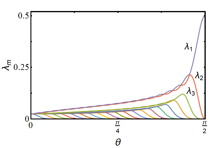
Figure 4: Entanglement spectrum of the history state (eigenvalues $\lambda_{1}\geq\lambda_{2}\geq\ldots$ of the reduced densities $\rho_{S}$ or $\rho_{T}$) obtained from the overlap matrix (50) for an initially localized particle and $N=40$ as a function of the coin operator parameter $\theta$.

For sufficiently large $N$ the eigenvalues of each block (identical for $N$ even) come essentially in almost degenerate pairs for $\theta$ not close to $\pi/2$, with the number of non-negligible eigenvalues decreasing with increasing $\theta$, as depicted in Fig. 4. The largest eigenvalue lies close to the Gershgorin upper bound, i.e., using Eq. (46),

$$\lambda_{\rm max}(\theta) \approx {\textstyle\frac{1}{N}[1+\sqrt{\frac{\tan\theta}{\pi}}\sum\limits_{n=1}^{\frac{N}{2}-1}\frac{|\cos(2n\theta+\pi/4)|}{\sqrt{n}}]}$$ (51a)

$$\approx {\textstyle\frac{1}{N}[1+\sqrt{\frac{\tan\theta}{2\pi}}H_{\frac{1}{2}}(\tfrac{N}{2}-1)]}$$ (51b)

$$\approx {\frac{1}{N}+\sqrt{\frac{\tan\theta}{N\pi}}\left[1+\frac{\zeta(\frac{1}{2})}{\sqrt{2N}}\right]}\,,$$ (51c)

where $H_{1/2}(m)=\sum_{n=1}^{m}\frac{1}{\sqrt{n}}$ ($\approx 2\sqrt{m}+\zeta(\frac{1}{2})$ for large $m$) is the generalized harmonic number ($\zeta(1/2)\approx-1.46$ is the Riemann zeta function at $1/2$). Thus, there is always a deviation $O(N^{-1/2})$ from the maximally mixed distribution, proportional to $\tan^{1/2}\theta$.

IV Relation with operator entanglement

IV.1 Entanglement of unitary operators

We will show here that the system-time entanglement entropy for the initially localized particle, which is independent of the initial (real) spin state, is the entanglement entropy of the global unitary operator which generates the quantum walk.

First, let us consider a complete set of local orthogonal operators $O_{i}^{S}$ ($O_{j}^{T}$) of the system (clock) satisfying

$${\rm Tr}_{S}\,[O_{i}^{S{\dagger}}O_{i^{\prime}}^{S}]=d_{S}\delta_{ii^{\prime}}\,,\;\;\;\;{\rm Tr}_{T}\,[O_{j}^{T{\dagger}}O_{j^{\prime}}^{T}]=d_{T}\delta_{jj^{\prime}}\,,$$ (52)

where $d_{S(T)}$ is the Hilbert space dimension of $S$ ($T$). Any operator ${\cal U}$ on the whole system can be expanded as

$${\cal U}=\sum_{i,j}{M}_{ij}\,O_{i}^{S}\otimes O_{j}^{T}\,,$$ (53)

where ${M}_{ij}=\frac{1}{d_{S}d_{T}}{\rm Tr}\,[(O_{i}^{\dagger}\otimes O_{j}^{\dagger})\,{\cal U}]$. Then $\frac{1}{d_{S}d_{T}}{\rm Tr}\,[{\cal U}^{\dagger}{\cal U}]=\sum_{i,j}|{M}_{ij}|^{2}={\rm Tr}[{M}^{\dagger}{M}]$. If ${\cal U}$ is unitary, ${\rm Tr}\,[{M}^{\dagger}{M}]=1$ and the $|{M}_{ij}|^{2}$ become standard probabilities.

Hence, in the same way as done for the history state, through the SVD ${M}=VDW^{\dagger}$, with $D_{mm^{\prime}}={\lambda}_{m}\delta_{mm^{\prime}}$ and $V$, $W$ unitary, we can also obtain the Schmidt representation of the operator ${\cal U}$,

$${\cal U}=\sum_{m=1}^{\tilde{n}_{s}}\sqrt{\tilde{\lambda}_{m}}\,\tilde{O}_{m}^{S}\otimes\tilde{O}_{m}^{T}\,,$$ (54)

where $\lambda_{m}$ are the eigenvalues of $M^{\dagger}M$ or $MM^{\dagger}$ and $\tilde{O}_{m}^{S}=\sum_{i}V_{im}O_{i}^{S}$, $\tilde{O}_{m}^{T}=\sum_{j}W^{*}_{jm}O_{j}^{T}$ are new local orthogonal operators satisfying (52), with $\tilde{n}_{s}$ the rank of $\tilde{M}$. If ${\cal U}$ is unitary the eigenvalues $\lambda_{m}$ are again standard probabilities ($\lambda_{m}\geq 0$, $\sum_{m}\lambda_{m}=1$). Thus, for a general trace-form entropy, the entanglement entropy of the unitary operator ${\cal U}$ can be defined as

$$E({\cal U})=\sum_{m}f(\lambda_{m})\,,$$ (55)

vanishing iff ${\cal U}$ is a product of local unitaries ($\tilde{n}_{s}=1$).

The analogy with state entanglement is straightforward if the Choi isomorphism for representing operators is employed. Any operator ${\cal U}$ on ${\cal H}_{ST}={\cal H}_{S}\otimes{\cal H}_{T}$ can be associated to a pure state $|{\cal U}\rangle$ in ${\cal H}_{ST}\otimes{\cal H}_{ST}$ given by

$$|{\cal U}\rangle=({\cal U}\otimes\mathbbm{1}_{ST})|\mathbbm{1}\rangle=\frac{1}{\sqrt{d_{S}d_{T}}}\sum_{\mu}({\cal U}|\mu\rangle)\otimes|\mu\rangle$$ (56)

where $|\mathbbm{1}\rangle=\frac{1}{\sqrt{d_{S}d_{T}}}\sum_{\mu}|\mu\rangle\otimes|\mu\rangle$ is a maximally entangled state in ${\cal H}_{ST}\otimes{\cal H}_{ST}$. In this way, an exact map for inner products is obtained:

$$\langle{\cal U}^{\prime}|{\cal U}\rangle=\frac{1}{d_{S}d_{T}}{\rm Tr}\,[{\cal U}^{\prime{\dagger}}{\cal U}]\,,$$ (57)

with $\langle{\cal U}|{\cal U}\rangle=1$ for a unitary operator ${\cal U}$. Thus, Eqs. (53)–(54) can be recast, noting that $|\mathbbm{1}\rangle=|\mathbbm{1}_{S}\rangle\otimes|\mathbbm{1}_{T}\rangle$, as

$$|{\cal U}\rangle = \sum_{i,j}M_{ij}|O_{i}^{S}\rangle\otimes|O^{T}_{j}\rangle=\sum_{m}\sqrt{\lambda_{m}}|\tilde{O}_{m}^{S}\rangle\otimes|\tilde{O}^{T}_{m}\rangle\;\;\;\;$$ (58)

with $|O_{i}^{S}\rangle=(O_{i}^{S}\otimes\mathbbm{1}_{S})|\mathbbm{1}_{S}\rangle=\frac{1}{d_{S}}\sum_{\mu}(O_{i}^{S}|\mu_{S}\rangle)\otimes|\mu_{S}\rangle$ and similarly for $|O_{j}^{T}\rangle$, such that $M_{ij}=(\langle O_{i}^{S}|\otimes\langle O_{j}^{T}|)|{\cal U}\rangle$. We can now rewrite (55) as

$$E({\cal U})=S(\rho^{\cal U}_{S})=S(\rho^{\cal U}_{T})\,,$$ (59)

where $\rho^{\cal U}_{S(T)}={\rm Tr}_{T(S)}\,|{\cal U}\rangle\langle{\cal U}|=\sum_{m}\lambda_{m}|\tilde{O}_{m}^{S(T)}\rangle\langle\tilde{O}_{m}^{S(T)}|$ are the local reduced densities derived from $|{\cal U}\rangle$. In particular, the quadratic entropy becomes

$$E_{2}({\cal U}) =1-{\rm Tr}\,(\rho_{S(T)}^{\cal U})^{2}=1\!-\!{\rm Tr}\,[(MM^{\dagger})^{2}]\,.$$ (60)

IV.2 Operator entanglement and quantum walk

If a system initially in a state $|\Psi_{0}\rangle$ undergoes a discrete unitary evolution through times $n=0,\ldots,N-1$ and states $|\Psi_{n}\rangle=U_{n}|\Psi_{0}\rangle$, its history state can be generated from an initial system-clock product state as (see Fig. 1)

$$|\text{\large$\Psi$}\rangle=\frac{1}{\sqrt{N}}\sum_{n=0}^{N-1}U_{n}|\Psi_{0}\rangle\otimes|n\rangle={\cal W}(|\Psi_{0}\rangle\otimes|\tilde{0}\rangle)\,,$$ (61)

where $|\tilde{0}\rangle=H^{\otimes m}|0\rangle=\frac{1}{\sqrt{N}}\sum_{n=0}^{N-1}|n\rangle$ and

$${\cal W}=\sum_{n=0}^{N-1}U_{n}\otimes|n\rangle\langle n|$$ (62)

is a controlled-$U_{n}$ unitary operator on the whole system. Its state representation (56) is

$$|{\cal W}\rangle=\frac{1}{\sqrt{N}}\sum_{n=0}^{N-1}|U_{n}\rangle\otimes|T_{n}\rangle$$ (63)

where $|T_{n}\rangle=(\sqrt{N}|n\rangle\langle n|\otimes\mathbbm{1})|\mathbbm{1}\rangle=|n\rangle\otimes|n\rangle$ and $|U_{n}\rangle=\frac{1}{\sqrt{d_{S}}}\sum_{\mu}(U_{n}|\mu_{S}\rangle)\otimes|\mu_{S}\rangle$. Therefore, the unitary operator ${\cal W}$ generating the history state from a product state can itself be represented as an operator history state (63).

The reduced operator state of the clock is here

$$\rho^{\cal W}_{T}={\rm Tr}_{S}|{\cal W}\rangle\langle{\cal W}|=\frac{1}{N}\sum_{n,n^{\prime}}\langle U_{n}|U_{n^{\prime}}\rangle|T_{n}\rangle\langle T_{n}|\,,$$ (64)

in full analogy with (27b), showing again that the entanglement of the generating operator (62)–(63),

$$E({\cal W})=S(\rho_{S}^{\cal W})=S(\rho_{T}^{\cal W})\,,$$ (65)

is fully determined by the overlaps $\langle U_{n^{\prime}}|U_{n}\rangle$. In the present random walk, $U_{n}=U^{n}$ and

$$\langle U_{n^{\prime}}|U_{n}\rangle=\frac{1}{2M}{\rm Tr}[U^{n-n^{\prime}}]\,,$$ (66)

is exactly the overlap (44)-(45)–(50) between the evolved system states for an initially localized particle with real initial spin state.

Thus, the operator entanglement (65) is exactly that of the previous system-clock history state for the initially localized particle, for any choice of entropy. In particular, the quadratic operator entanglement

$$E_{2}({\cal W})=1-{\rm Tr}\,(\rho_{T}^{\cal W})^{2}=1-\frac{1}{N^{2}}\sum_{n,n^{\prime}}|\langle U_{n^{\prime}}|U_{n}\rangle|^{2}\,,$$ (67)

is just the quadratic $S$–$T$ entropy (47). And the entanglement spectrum of ${\cal W}$ coincides with that of the history state (Fig. 4).

The quadratic entropy (67) has an additional meaning: It determines the entangling power of the unitary operator ${\cal W}$, i.e. the average quadratic entanglement $E_{2}(S,T)$ it generates when applied to initial product system-clock states:

$$\langle E_{2}(S,T)\rangle = \int_{\cal H}(1-{\rm Tr}\,\rho_{S}^{2})\,d\Psi_{0}$$ (68)

$$= \frac{d_{S}}{d_{S}+1}E_{2}({\cal W}),$$

with the average taken over the whole set of initial system states $|\Psi_{0}\rangle$ with the Haar measure $d\Psi_{0}$ Boette and Rossignoli (2018). Thus, for $d_{S}\gg 1$ the quadratic $S$–$T$ entanglement entropy (47), equal to (67), is very close to the average value (68).

IV.3 Spin history states in the quantum walk

If we now consider as system only the spin degree of freedom, we first notice from Eq. (13) that for a particle initially localized at $x=0$, the state after $n$ steps

$$|\Psi_{n}\rangle=\frac{1}{\sqrt{M}}\sum_{k}|k\rangle\otimes U_{k}^{n}|\chi_{0}\rangle\,,$$ (69)

is exactly a spin history state, with respect to the momentum states $|k\rangle$. The “evolution” operators are here the $k$-projected unitaries $U_{k}^{n}$ acting on the spin, having a nontrivial $k$-dependence. Thus, the spin-position entanglement at step $N$ is that of a spin history state. The same holds for any initial localization $x_{0}$ ($|k\rangle\rightarrow e^{-i2\pi kx_{0}/M}|k\rangle$).

Therefore, its average $\langle E_{2}(s,p)\rangle$ over all initial spin states is determined by the entanglement of the operator $U^{n}$ generating such spin history [from the initial product state $|\Psi_{0}\rangle=(\frac{1}{\sqrt{M}}\sum_{k}|k\rangle)|\chi_{0}\rangle$], itself an operator history state, as is apparent from Eq. (10a):

$$U^{n}=\sum_{k=0}^{M-1}|k\rangle\langle k|\otimes U_{k}^{n}\,.$$ (70)

The associated operator state is $\frac{1}{\sqrt{M}}\sum_{k}|P_{k}\rangle|U_{k}^{n}\rangle$ with $|P_{k}\rangle=|k\rangle\otimes|k\rangle$ and $|U_{k}^{n}\rangle=\frac{1}{\sqrt{2}}\sum_{\nu=\pm}U_{k}^{n}|\nu\rangle|\nu\rangle$ ($|\nu=\pm\rangle$ are orthogonal spin states). Its entanglement is then determined by the overlaps (see Eqs. (10) and (74) below)

$$\langle U_{k^{\prime}}^{n}|U_{k}^{n}\rangle = \tfrac{1}{2}{\rm Tr}\,[U_{k^{\prime}}^{-n}\,U_{k}^{n}]\,.$$ (71)

While the unitaries $U_{k}^{n}$ belong to a four-dimensional space spanned by the identity and the three Pauli operators, limiting the Schmidt rank of (70) to $n_{s}\leq 4$ $\forall$ $M$, they actually live within a three-dimensional subspace spanned by the identity $\mathbbm{1}_{s}$, the coin operator $\sigma_{\theta}\equiv C$ and the orthogonal Pauli operator $\sigma_{y}$: From (7)–(8) we see that

$$U_{k}=\cos\phi_{k}\,\sigma_{\theta}-i\sin\phi_{k}\exp[i\theta\sigma_{y}]\,,$$ (72)

since $\sigma_{z}\sigma_{\theta}=\cos\theta\,\mathbbm{1}_{s}+i\sin\theta\,\sigma_{y}$. And from (10b) and (72) it follows that

$$|s_{k}^{\pm}\rangle\langle s_{k}^{\pm}| = \tfrac{1}{2}(\mathbbm{1}\pm\sigma_{k})\,,$$ (73a)

$$\sigma_{k} = \frac{\cos\phi_{k}}{\cos\omega_{k}}\sigma_{\theta}+\frac{\sin\phi_{k}\sin\theta}{\cos\omega_{k}}\sigma_{y}\,,$$ (73b)

with $\sigma_{k}^{2}=\mathbbm{1}$. Hence all powers

$$U_{k}^{n} = e^{-in\omega_{k}}|s_{k}^{+}\rangle\langle s_{k}^{+}|+(-1)^{n}e^{in\omega_{k}}|s_{k}^{-}\rangle\langle s_{k}^{-}|$$ (74a)

$$= \cos(n\omega_{k})\mathbbm{1}-i\sin(n\omega_{k})\sigma_{k}\;\;\;\;\;\;\;(n\;{\rm even})\,,$$

$$= -i\sin(n\omega_{k})\mathbbm{1}+\cos(n\omega_{k})\sigma_{k}\;\;\;\;\;(n\;{\rm odd})\,,$$ (74b)

are spanned just by $\{\mathbbm{1}_{s},\sigma_{\theta},\sigma_{y}\}$ $\forall$ $k,n$, with ${\rm Tr}\,\sigma_{\theta}\sigma_{y}=0$. This entails a Schmidt rank $n_{s}\leq 3$ of the $n^{\rm th}$ power (70), implying at most $3$ non-zero eigenvalues ${\lambda}_{m}$ in its associated entanglement spectrum, as seen in Fig. 5, and a von Neumann entanglement entropy $E(U^{n})\leq\log_{2}3$.

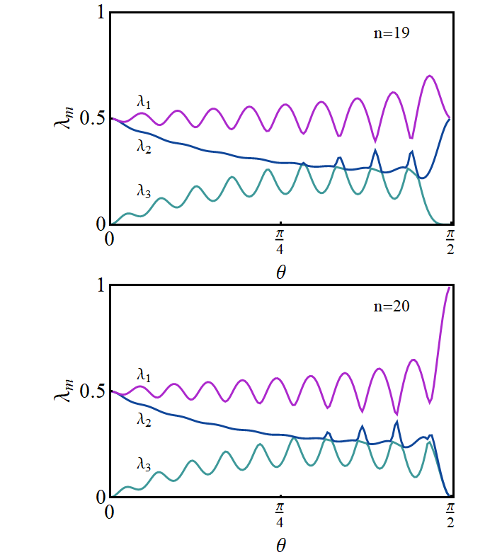
Figure 5: Entanglement spectrum of the unitary operator (70) for an odd (top) and even (bottom) $n$ as a function of the coin operator parameter $\theta$.

For $U$ itself ($n=1$) just $\{\sigma_{\theta},e^{i\theta\sigma_{y}}\}$ are needed as seen from (72), implying $n_{s}=2$, as also evident from the original expression (3). Its entanglement spectrum is just $(1/2,1/2,0)$. However, for $n\geq 2$ the rank is $n_{s}=3$ if $\theta\in(0,\pi/2)$ (and $M>3$). Exceptions occur for $\theta=0$, in which case $\omega_{k}=\phi_{k}$ and $\sigma_{k}=\sigma_{\theta}=\sigma_{z}$ $\forall\,k$, leading to $n_{s}=2$ and an entanglement spectrum $(1/2,1/2,0)$ $\forall$ $n\geq 1$, as verified in Fig. 5, and also for $\theta=\pi/2$, where $\omega_{k}=0$ $\forall$ $k$ and $\sigma_{\theta}=\sigma_{x}$, leading to $n_{s}=1$ $\forall$ $n$ even (as $U_{k}^{n}=\mathbbm{1}$ $\forall$ $k$) and $n_{s}=2$ for $n$ odd (as $U_{k}^{n}=\sigma_{k}$), with spectrum $(1/2,1/2,0)$, as also seen in Fig. 5.

Therefore, the entangling power of $U^{n}$ remains bounded by this rank $n_{s}\leq 3$: Rescaling the quadratic entropy as $S_{2}(\rho)=2(1-{\rm Tr}\,\rho^{2})$, such that $S_{2}(\rho)=1$ for a maximally mixed single spin state, it implies $E_{2}(U^{n})\leq 4/3$. Hence, applying the relation (68) to the spin history, the average over all initial spin states of the spin-position entanglement after $n$ steps satisfies

$$\langle E_{2}(s,p)\rangle=(2/3)E_{2}(U^{n})\leq 8/9\,.$$ (75)

This bound is obviously lower than the maximum $\langle E_{2}(s,p)\rangle=1$ reached for a full rank maximally entangled operator $U_{n}$ ($E_{2}(U_{n})=3/2$ for the rescaled $S_{2}$), for which $|\Psi_{n}\rangle$ in  (69) would be maximally entangled ($E_{2}(s,p)=1$) for any spin state $|\chi_{0}\rangle$, in agreement with the general results of Boette and Rossignoli (2018). The variation of $\langle E_{2}(s,p)\rangle\propto E_{2}(U)$ with $\theta$ is depicted in Fig. 6.

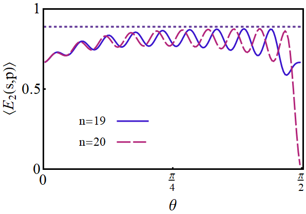
Figure 6: The average over all initial spin states of the spin-position quadratic entanglement entropy $\langle E_{2}(s,p)\rangle=(2/3)E_{2}(U^{n})$ (Eq. (75)), as a function of the coin operator parameter $\theta$, for the even and odd cases of Fig. 5. The dotted line indicates the upper bound $8/9$.

Similarly, the full history state (18) for the initially localized particle can also be regarded, when viewed from the spin, as a spin history state with respect to a composite clock, comprising both the original clock and the position degrees of freedom:

$$|\text{\large$\Psi$}\rangle=\frac{1}{\sqrt{NM}}\sum_{k,n}|kn\rangle\otimes U_{k}^{n}|\chi_{0}\rangle,$$ (76)

where $|kn\rangle=|k\rangle\otimes|n\rangle$ and for clarity we have altered the order in the tensor product. In this case the unitary operator generating the full spin history is

$${\cal W}_{s}=\sum_{k,n}|kn\rangle\langle kn|\otimes U_{k}^{n}\,.$$ (77)

The average (over all initial spin states) $\langle E_{2}(s,pT)\rangle$ of the spin–rest entanglement in the state (76) is then determined by the entanglement of the operator (77), in turn determined by the full set of overlaps

$$\langle U_{k^{\prime}}^{n^{\prime}}|U_{k}^{n}\rangle = \tfrac{1}{2}{\rm Tr}\,[U_{k^{\prime}}^{-n^{\prime}}\,U_{k}^{n}]\,,$$ (78)

for $0\leq k,k^{\prime}\leq M$, $0\leq n,n^{\prime}\leq N-1$.

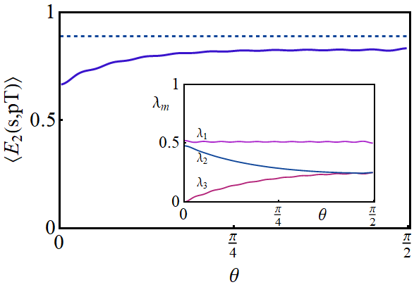
Figure 7: Average over all initial spin states of the spin–rest quadratic entanglement entropy, $\langle E_{2}(s,pT)\rangle=(2/3)E_{2}({\cal W}_{s})$ (Eq. (79)), as a function of the coin operator parameter $\theta$, for $N=20$. The dotted line indicates the upper bound $8/9$. Inset: Entanglement spectrum of the unitary operator ${\cal W}_{s}$, Eq.  (77) generating the full spin history, as a function of the coin operator parameter $\theta$.

Nonetheless, since all $U_{k}^{n}$ are spanned just by $\{\mathbbm{1}_{s},\sigma_{\theta},\sigma_{y}\}$ (Eq. (72)), the Schmidt rank of (77) is again $n_{s}=3$ (or $n_{s}\leq 3$ in general), and the previous bound, i.e. $E_{2}({\cal W}_{s})\leq 4/3$ still holds. This entails again

$$\langle E_{2}(s,pT)\rangle=(2/3)E_{2}({\cal W}_{s})\leq 8/9\,.$$ (79)

This average is depicted as a function of $\theta$ in Fig. 7, together with the entanglement spectrum of ${\cal W}_{s}$.

V Conclusions

We have analyzed the history state formalism in the context of discrete QW. The history state captures the whole evolution of the system, enabling for instance the evaluation of time averages as single quantum expectation values. It satisfies a timeless eigenvalue equation and can be generated through a quantum circuit from an initial system-clock product state. The associated system-clock entanglement entropy is a measure of the number of orthogonal system states visited in the whole QW and is fully determined by the overlaps between the evolved states. Stationary system states then lead to separable history states, while QW in which the system evolves into a new orthogonal state at each step correspond to maximally entangled history states.

We have then shown that in one dimensional QW with real Hadamard-type coin operators, such entanglement is strictly independent of the initial spin orientation for real initial states with definite position parity. We also analyzed its connection with operator entanglement, showing that in the standard case of an initially localized particle it coincides exactly with the entanglement of the unitary operator generating the whole QW. Exact analytic results for overlaps and quadratic entropies as a function of the number $N$ of steps and the coin parameter were as well derived, including asymptotic expressions for large $N$. The latter show a monotonously decreasing entropy with increasing coin operator parameter $\theta\in[0,\pi/2]$, with $S_{2}(0)-S_{2}(\theta)\propto\tan\theta\frac{\ln N}{N}$ for the quadratic entropy. The associated history state entanglement spectrum shows, accordingly, a decreasing rank for increasing $\theta$, with a deviation $O(\frac{\tan\theta}{N})^{\frac{1}{2}}$ from $N^{-1}$ in the largest eigenvalue.

Finally, we have examined the QW from the spin perspective, showing that for an initially localized particle it is also described by a history state with a composite clock and a $k$-dependent unitary. The average over all initial spin states of the ensuing spin-rest entanglement can then be related to that of the global unitary generating this history. For the present Hadamard-type coin operator it has a limited rank with just three non-zero eigenvalues in its entanglement spectrum, leading to a bounded average spin-rest entanglement.

In summary, the history state formalism provides a novel perspective for analyzing QW. The associated system-time entanglement entropy constitutes a new measure for characterizing the whole evolution, which could be employed, for instance, in relation with the identification of dynamical phase transitions Wang2 et al. (2019) and topological phases Kitagawa et al. (2010); Xu et al. (2019); cardano et al. (2020); QQW et al. (2020); colandrea et al. (2022), of great current interest. The formalism also opens the way to efficient direct evaluation of time averages and quadratic entanglement entropies through its simulation in a quantum circuit Boette et al. (2016); Boette and Rossignoli (2018); Pabón et al. (2019), while a variational determination of the history state becomes as well possible. Finally, the extension of the formalism to open systems with nonunitary dynamics and to more complex scenarios is in principle feasible and is currently under investigation.

Appendix A Quadratic entanglement entropy summation

The sum for the quadratic entanglement entropy (47b) can be done exactly for large $n$ using the approximation (46) and neglecting terms $O(n^{-\frac{3}{2}})$. This yields

$$E_{2}(S,T) \approx 1-[1+\tfrac{\tan\theta}{\pi}F(N,\theta)]/N\,,$$ (80)

with

$$F(N,\theta) = 2\sum_{n=1}^{\eta}(\tfrac{1}{n}-\tfrac{2}{N})\cos^{2}(2n\theta+\pi/4)$$ (82)

$$= H(\eta)+{\rm Im}[e^{4i\theta\eta}L(e^{4i\theta},\eta)]+2\theta-\tfrac{\pi}{2}$$

$$-\tfrac{2}{N}[\eta-\tfrac{\sin(2\theta(\eta+1))\sin(2\theta\eta)}{\sin(2\theta)}]\,,$$

where $\eta=\lfloor\frac{N-1}{2}\rfloor$, $H(\eta)=\sum_{n=1}^{\eta}1/n$ is the harmonic number and $L(z,\eta):=\sum_{k=1}^{\infty}{z^{k}}/(k+\eta)$ is directly related to the Lerch zeta function Abramowitz and Stegun (1965).

References

- Aharonov et al. (1993) Y. Aharonov, L. Davidovich, and N. Zagury, “Quantum random walks,” Phys. Rev. A 48, 1687 (1993).
- Feynman et al. (2010) R.P. Feynman, A.R. Hibbs, and D.F. Styer, Quantum mechanics and path integrals (Courier Corp., 2010).
- Kempe (2003) J. Kempe, “Quantum random walks: An introductory overview,” Contemp. Phys. 44, 307 (2003).
- Venegas-Andraca (2012) S. E. Venegas-Andraca, “Quantum walks: a comprehensive review,” Quantum Inf. Process. 11, 1015 (2012).
- Ambainis (2003) A. Ambainis, “Quantum walks and their algorithmic applications,” Int. J. Quantum Inform. 1, 507 (2003).
- Shenvi et al. (2003) N. Shenvi, J. Kempe, and K. Birgitta Whaley, “Quantum random-walk search algorithm,” Phys. Rev. A 67, 052307 (2003).
- Childs and Goldstone (2004) A. M. Childs and J. Goldstone, “Spatial search by quantum walk,” Phys. Rev. A 70, 022314 (2004).
- Berry and Wang (2010) S. D. Berry and J. B. Wang, “Quantum-walk-based search and centrality.” Phys. Rev. A 82, 042333 (2010).
- Grover (1997) L.K. Grover, “Quantum mechanichs helps in searching for a needle in a haystack,” Phys. Rev. Lett. 79, 325 (1997).
- Childs (2009) A.M. Childs, “Universal computation by quantum walk,” Phys. Rev. Lett. 102, 180501 (2009).
- Lovett et al. (2010) N. B. Lovett et al., “Universal quantum computation using the discrete-time quantum walk,” Phys. Rev. A 81, 042330 (2010).
- Sánchez-Burillo et al. (2012) E. Sánchez-Burillo, J. Duch, J. Gómez-Gardeñes, and D. Zueco, “Quantum navigation and ranking in complex networks.” Sci. Rep. 2, 605 (2012).
- Lloyd (1996) S. Lloyd, “Universal quantum simulators.” Science 273, 1073 (1996).
- Berry and Childs (2012) A. M. Childs and D. W. Berry, “Black-box hamiltonian simulation and unitary implementation.” Quantum Inf. Comput. 12, 29 (2012).
- Schreiber et al. (2012) A. Schreiber et al., “A 2d quantum walk simulation of two-particle dynamics.” Science 336, 55 (2012).
- Qiang et al. (2016) X. Qiang et al., “Efficient quantum walk on a quantum processor.” Nat. Commun. 7, 11511 (2016).
- Engel et al. (2007) G. Engel et al., “Evidence for wavelike energy transfer through quantum coherence in photosynthetic systems.” Nature 446, 782 (2007).
- Rebentrost et al. (2009) P. Rebentrost et al., “Environment-assisted quantum transport.” New J. Phys. 11, 033003 (2009).
- Karski et al. (2009) M. Karski et al., “Quantum walk in position space with single optically trapped atoms,” Science 325, 174 (2009).
- Preiss et al. (2015) P.M. Preiss et al., “Strongly correlated quantum walks in optical lattices,” Science 347, 1229 (2015).
- Mugel et al. (2016) S. Mugel et al., “Topological bound states of a quantum walk with cold atoms,” Phys. Rev. A 94, 023631 (2016).
- Schmitz et al. (2009) H. Schmitz et al., “Quantum walk of a trapped ion in phase space,” Phys. Rev. Lett. 103, 090504 (2009).
- Zähringer et al. (2010) F. Zähringer et al., “Realization of a quantum walk with one and two trapped ions,” Phys. Rev. Lett. 104, 100503 (2010).
- Gräfe et al. (2016) M. Gräfe et al., “Integrated photonic quantum walks,” J. Opt. 18, 103002 (2016).
- Flamini et al. (2019) F. Flamini, N. Spagnolo, and F. Sciarrino, “Photonic quantum information processing: a review,” Rep. Prog. Phys. 82, 016001 (2019).
- Wang2 et al. (2019) K. Wang et al., “Simulating dynamic quantum phase transitions in photonic quantum walks,” Phys. Rev. Lett. 122, 020501 (2019).
- Xu et al. (2019) X.Y. Xu et al., “Measuring the winding number in a large-scale chiral quantum walk,” Phys. Rev. Lett. 120, 260501 (2018).
- cardano et al. (2020) A. D’Errico et al., “Two-dimensional topological quantum walks in the momentum space of structured light,” Optica 7, 108 (2020).
- QQW et al. (2020) Q.Q. Wang et al., “Robustness of entanglement as an indicator of topological phases in quantum walks,” Optica 7, 53 (2020).
- colandrea et al. (2022) F. Di Colandrea et al., “Ultra-long photonic quantum walks via spin-orbit metasurfaces,” arXiv:2203.15051 (2022) .
- Carneiro et al. (2005) O. Carneiro et al., “Entanglement in coined quantum walks on regular graphs,” New. J. Phys. 7, 156 (2005).
- Venegas-Andraca et al. (2005) S. E. Venegas-Andraca, J. L. Ball, K. Burnett, and S. Bose, “Quantum walks with entangled coins,” New. J. Phys. 7, 221 (2005).
- Abal et al. (2006) G. Abal, R. Siri, A. Romanelli, and R. Donangelo, “Quantum walk on the line: Entanglement and nonlocal initial conditions,” Phys. Rev. A 73, 042302 (2006), Erratum: ibid, Phys. Rev. A 73, 069905 (2006).
- Omar et al. (2006) Y. Omar, N. Paunković, L. Sheridan, and S. Bose, “Quantum walk on the line with two entangled particles,” Phys. Rev. A 74, 042304 (2006).
- Maloyer and Kendon (2007) O. Maloyer, V. Kendon, “Decoherence vs. entanglement in coined quantum walks,” New. J. Phys. 9, 87 (2007).
- Annabestani et al. (2010) A. Annabestani, M. R. Abolhasani, and G. Abal, “Asymptotic entanglement in 2d quantum walks,” J. Phys. A 43, 075301 (2010).
- Romanelli (2010) A. Romanelli, “Distribution of chirality in the quantum walk: Markov process and entanglement,” Phys. Rev. A 81, 062349 (2010).
- Ide et al. (2011) Y. Ide, N. Konno, and T. Machida, “Entanglement for discrete-time quantum walks on the line,” Quant. Inf. Comp. 11, 855 (2011).
- Allés et al. (2012) B. Allés, S. Gündüç, and Y. Gündüç, “Maximal entanglement from quantum random walks,” Quant. Inf. Process. 11, 211 (2012).
- Vieira et al. (2014) R. Vieira, E.P.M. Amorim, and G. Rigolin, “Entangling power of disordered quantum walks,” Phys. Rev. A 89, 042307 (2014), “Dynamically disordered quantum walk as a maximal entanglement generator”, Phys. Rev. Lett. 111 180503 (2013).
- Orthey and Amorim (2017) A. C. Orthey and E.P.M. Amorim, “Asymptotic entanglement in quantum walks from delocalized initial states,” Quantum Inf. Process. 16, 224 (2017).
- Page and Wootters (1983) D.N. Page and W.K. Wootters, “Evolution without evolution: Dynamics described by stationary observables,” Phys. Rev. D 27, 2885 (1983), W.K. Wootters, “Time replaced by quantum correlations”, Int. J. Th. Phys. 23, 701 (1984).
- Rovelli (1990) C. Rovelli, “Quantum mechanics without time: a model,” Phys. Rev. D 42, 2638 (1990).
- Isham (1994) C. J. Isham, “Quantum logic and the histories approach to quantum theory,” J. Math. Phys. 35, 2157 (1994).
- Giovannetti et al. (2015) V. Giovannetti, S. Lloyd, and Maccone L., “Quantum time,” Phys. Rev. D 92, 045033 (2015).
- Moreva et al. (2014) E. Moreva, G. Brida, M. Gramegna, V. Giovannetti, L. Maccone, and M. Genovese, “Time from quantum entanglement: An experimental illustration,” Phys. Rev. A 89, 052122 (2014).
- McClean and Aspuru-Guzik (2015) J.R. McClean and A. Aspuru-Guzik, “Clock quantum Monte Carlo technique: An imaginary-time method for real-time quantum dynamics,” Phys. Rev. A 91, 012311 (2015); J.R. McClean, J.A. Parkhill, A. Aspuru-Guzik, “Feynman’s clock, a new variational principle, and parallel-in-time quantum dynamics”, PNAS 110, E3901 (2013).
- Boette et al. (2016) A. Boette, R. Rossignoli, N. Gigena, and M. Cerezo, “System-time entanglement in a discrete-time model,” Phys. Rev. A 93, 062127 (2016).
- Boette and Rossignoli (2018) A. Boette and R. Rossignoli, “History states of systems and operators,” Phys. Rev. A 98, 032108 (2018).
- DeWitt (1967) B. DeWitt, “Quantum theory of gravity. I. The canonical theory,” Phys. Rev. 160, 1113 (1967).
- Dias and Parisio (2017) E.O. Dias and F. Parisio, “Space-time-symmetric extension of nonrelativistic quantum mechanics,” Phys. Rev. A 95, 032133 (2017).
- Nikolova et al. (2018) A. Nikolova et al., “Relational time in anyonic systems,” Phys. Rev. A 97, 030101(R) (2018).
- Coles et al. (2019) P.J. Coles, V. Katariya, S. Lloyd, I. Marvian, and M.M. Wilde, “Entropic energy-time uncertainty relation,” Phys. Rev. Lett. 122, 100401 (2019).
- Pabón et al. (2019) D. Pabón et al., “Parallel-in-time optical simulation of history states,” Phys. Rev. A 99, 062333 (2019).
- Cirac et al. (2022) S. Barison, F. Vicentini, I. Cirac, and G. Carleo, “Variational dynamics as a ground-state problem on a quantum computer,” arXiv:2204.03454 (2022).
- Gambini et al. (2009) R. Gambini, R. A. Porto, J. Pullin, and S. Torterolo, “Conditional probabilities with Dirac observables and the problem of time in quantum gravity,” Phys. Rev. D 79, 041501(R) (2009).
- Zhao et al. (2018) Z. Zhao et al., “Geometry of quantum correlations in space-time,” Phys. Rev. A 98, 052312 (2018).
- Diaz and Rossignoli (2019) N. L. Diaz and R. Rossignoli, “History state formalism for Dirac’s theory,” Phys. Rev. D 99, 045008 (2019).
- Diaz et al. (2019) N. L. Diaz, J. M. Matera, and R. Rossignoli, “History state formalism for scalar particles,” Phys. Rev. D 100, 125020 (2019); N.L. Diaz, J.M. Matera, R. Rossignoli, “Spacetime quantum actions”, Phys. Rev. D 103, 065011 (2021).
- Ambainis et al. (2001) A. Ambainis, E. Bach, A. Nayak, A. Vishwanath, and J. Watrous, “One-dimensional quantum walks,” in Proceedings of the Thirty-third Annual ACM Symposium on Theory of Computing, STOC’01, ACM Press, NY, 37 (2001).
- Konno (2002) N. Konno, “Quantum random walks in one dimension,” Quantum Inf. Proc. 1, 345 (2002).
- Tregenna et al. (2003) B. Tregenna, W. Flanagan, R. Maile, and V. Kendon, “Controlling discrete quantum walks: coins and initial states,” New J. Phys. 5, 83 (2003).
- Tsallis (2009) C. Tsallis, Introduction to Non-Extensive Statistical Mechanics (Springer–Verlag, N.Y., 2009).
- Nakazato et al. (2012) H. Nakazato, T. Tanaka, K. Yuasa, G. Florio, and S. Pascazio, “A measurement scheme for purity based on two-body gates,” Phys. Rev. A 85, 042316 (2012).
- Beck and Schlögl (1993) C. Beck and F. Schlögl, Thermodynamic of Chaotic Systems (Cambridge Univ. Press, UK, 1993).
- Abramowitz and Stegun (1965) M. Abramowitz and I.A. Stegun, eds., Handbook of Mathematical Functions with Formulas, Graphs, and Mathematical Tables, Applied Mathematics Series, Vol. 55 (Dover Publications, 1965); F.W. Olver, D.W. Lozier, R. Boisvert, C.W. Clark eds, NIST Handbook of Mathematical Functions, Cambridge Univ. Press (2010).
- Kitagawa et al. (2010) T. Kitagawa, M. S. Rudner, E. Berg, and E. Demler, “Exploring topological phases with quantum walks,” Phys. Rev. A 82, 033429 (2010).