Two-site anyonic Josephson junction

Abstract

Anyons are particles with intermediate quantum statistics whose wavefunction acquires a phase $e^{i\theta}$ by particle exchange. Inspired by proposals of simulating anyons using ultracold atoms trapped in optical lattices, we study a two-site anyonic Josephson junction, i.e. anyons confined in a one-dimensional double-well potential. We show, analytically and numerically, that many properties of anyonic Josephson junctions, such as Josephson frequency, imbalanced solutions, macroscopic quantum self-trapping, coherence visibility, and condensate fraction, crucially depend on the anyonic angle $\theta$. Our theoretical predictions are a solid benchmark for near future experimental quantum simulations of anyonic matter in double-well potentials.

I Introduction

In three spatial dimensions the quantum concept of particle indistinguishability leads to two superselection sectors: one sector related to bosonic particles whose wavefunction is symmetric by the exchange of two particles, and the other sector related to fermionic particles whose wavefunction is anti-symmetric by the exchange of two particles. In 1982 it was conjectured by Wilczek wilczek the existence of two-dimensional quasi-particles, called anyons, whose wavefunction acquires a phase $e^{i\theta}$ by particle exchange, with $\theta\in[0,\pi]$. Indeed, the fractional quantum Hall effect in a two-dimensional electron system can be explained in terms of anyons laughlin ; halperin . The physics of anyons remained confined to the two-dimensional case until a model of fractional statistics in arbitrary dimension was proposed by Haldane haldane , also on the basis of previous theoretical investigations gentile . Triggered by the experimental realization of artificial spin-orbit and Rabi couplings with atoms spielman1 ; spielman2 , sophisticated experimental techniques have been proposed roncaglia ; santos ; strater ; pelster ; zhang to simulate anyons by using ultracold atoms trapped in one-dimensional optical lattices veronica ; pelster2 .

In this paper we consider a two-site anyonic Hubbard model, which describes $N$ anyons confined in a quasi one-dimensional double-well potential. This system can be also seen as the anyonic analog of the familiar Josephson junction josephson ; barone ; vari . By using the Jordan-Wigner transformation and coherent states we derive dynamical equations for the relative phase and population imbalance of the anyonic system. These equations crucially depend on the anyonic angle $\theta$ and they reduce to the familiar ones of bosonic Josephson junctions smerzi ; albiez for $\theta=0$. We show analytically the role of the anyonic angle $\theta$ on stationary configurations, Josephson frequecy, solution with non-zero imbalance, and macroscopic quantum self-trapping. We also consider many-body quantum properties of the exact ground state finding that the coherence visibility and the condensate fraction are strongly affected by the anyonic angle, while the entanglement entropy is not.

II The Model

Anyons are quasi-particles whose statistics interpolate between fermions and bosons depending on the angle $\theta\in[0,\pi]$. In the one-dimensional case, creation $\hat{a}_{j}^{\dagger}$ and annihilation $\hat{a}_{j}$ operators of anyons on the site $j$ satisfy the following commutation rules

$$\hat{a}_{j}\hat{a}^{+}_{k}-e^{-i\theta sgn(j-k)}\hat{a}_{k}^{+}\hat{a}_{j}=\delta_{jk}\,,$$ (1)

$$\hat{a}_{j}\hat{a}_{k}-e^{i\theta sgn(j-k)}\hat{a}_{k}\hat{a}_{j}=0\,,$$ (2)

with $i=\sqrt{-1}$ the imaginary unit and $sgn(x)$ the sign function such that $sgn(0)=0$. Clearly, for $\theta=0$ or $\theta=\pi$ one recovers the familar commutation rules of bosons or fermions. The anyons with the statistical exchange phase $\theta=\pi$ are actually pseudo-fermions, i.e. they are fermions off-site but bosons on-site.

In this paper we want to analyze anyonic Josephson junctions, which can be modelled by the two-site anyon-Hubbard Hamiltonian

$$\hat{H}=-J(\hat{a}^{\dagger}_{1}\hat{a}_{2}+\hat{a}^{\dagger}_{2}\hat{a}_{1})+\sum_{j=1,2}{U\over 2}\bigl{[}\hat{a}_{j}^{+}{\hat{a}}_{j}(\hat{a}_{j}^{+}\hat{a}_{j}-1)\bigl{]}\,,$$ (3)

where $J$ and $U$ are, respectively, the familiar tunneling (hopping) energy and on-site energy veronica . By using the Jordan-Wigner transformation roncaglia

$$\hat{a}_{1}=\hat{b}_{1}e^{i\theta\hat{N}_{2}}\qquad\hat{a}_{2}=\hat{b}_{2}\;,$$ (4)

we map anyons into bosons, with $\hat{b}_{j}$ and $\hat{b}_{j}^{+}$ annihilation and creation operators satisfying bosonic commutation rules, and $\hat{N}_{j}={\hat{b}}^{+}_{j}{\hat{b}}_{j}$ the number operator ($j=1,2$). Notice that ${\hat{b}}^{+}_{j}{\hat{b}}_{j}={\hat{a}}^{+}_{j}{\hat{a}}_{j}$. The Hamiltonian (3) then becomes

$$\hat{H}=-J(e^{-i\theta\hat{N}_{2}}\hat{b}^{\dagger}_{1}\hat{b}_{2}+\hat{b}^{\dagger}_{2}\hat{b}_{1}e^{i\theta\hat{N}_{2}})+\sum_{j=1,2}{U\over 2}\bigl{[}\hat{N}_{j}(\hat{N}_{j}-1)\bigl{]}\,.$$ (5)

Quite remarkably this $\theta$-dependent Bose-Hubbard Hamiltonian could be realized experimentally by trapping bosonic atoms in a quasi-1D optical double-well potential. In particular, the $\theta$ terms could be obtained by using an assisted Raman-tunneling scheme roncaglia ; santos or, alternatively, by a combination of lattice tilting and a periodic driving strater .

III Mean-field analysis with coherent states

We want to investigate the time evolution of the anyonic system. The time evolution of a generic quantum state $|\psi(t)\rangle$ of the system described by the Hamiltonian is given by the Schrödinger equation

$$i\hbar\frac{\partial}{\partial t}|\psi(t)\rangle=\hat{H}|\psi(t)\rangle\;.$$ (6)

This time evolution equation can be derived by minimizing of the action

$$S=\int dt\langle\psi(t)|\left(i\hbar\frac{\partial}{\partial t}-\hat{H}\right)|\psi(t)\rangle\;$$ (7)

characterized by the Lagrangian

$$L=\langle\psi(t)|i\hbar\frac{\partial}{\partial t}|\psi(t)\rangle-\langle\psi(t)|\hat{H}|\psi(t)\rangle\;.$$ (8)

A simple, but meaningful, mean-field approach is based on coherent states, which are eigenstates of the bosonic annihilation operator, namely

$$\hat{b}_{j}|{\beta_{j}}\rangle = \beta_{j}|{\beta_{j}}\rangle$$ (9)

$$\langle{\beta_{j}}|\hat{b}_{j}^{\dagger} = \beta_{j}^{*}\langle{\beta_{j}}|$$ (10)

where $j=1,2$ and $\beta_{j}\in\mathbb{C}$. These Glauber coherent states are not eigenstates of number operators but there are extremely reliable in describing many-body properties of bosonic Josephson junctions in the case of a large number $N$ of bosons ($N\gg 1$) under the condition $|U/(2J)|\ll N$ sala2021 . From these definitions it follows that $\langle\beta_{j}|{\hat{b}_{j}^{\dagger}\hat{b}_{j}}|\beta_{j}\rangle=|\beta_{j}|^{2}$. Moreover,

$$|\beta_{j}\rangle=e^{-\frac{1}{2}|\beta_{j}(t)|^{2}}e^{\beta_{j}\hat{b}_{j}^{\dagger}}|0\rangle\;,$$ (11)

where $|0\rangle$ is the vacuum state. In the Euler representation the complex eigenvalue $\beta_{j}(t)$ reads

$$\beta_{j}(t)=\sqrt{N_{j}(t)}\,e^{i\phi_{j}(t)}\;,$$ (12)

where $N_{j}(t)=|\beta_{j}(t)|^{2}$ is the average number of bosons in the $j$-th site at time $t$ and $\phi_{j}(t)$ is the corresponding bosonic phase.

By using these coherent states, the state $|\psi(t)\rangle$ is given by $|\psi(t)\rangle=|\beta_{1}(t)\rangle|\beta_{2}(t)\rangle$, and the Lagrangian of Eq. (8) becomes

$$L = \hbar(N_{1}-N_{2})({\dot{\phi}}_{2}-{\dot{\phi}}_{1})$$ (13)

$$+ 2J\sqrt{N_{1}N_{2}}\cos{(\phi_{2}-\phi_{1}-N_{2}\theta)}$$

$$- \frac{U}{4}\left(N^{2}_{1}+N^{2}_{2}\right)\;.$$

Let us now introduce the population imbalance $z(t)$ and the phase difference $\phi(t)$

$$z(t) = \frac{N_{1}(t)-N_{2}(t)}{N}$$ (14)

$$\phi(t) = \phi_{2}(t)-\phi_{1}(t)$$ (15)

where $N=N_{1}(t)+N_{2}(t)$ is constant. It is then possible to rewrite Eq. (13) in terms of the variables just introduced, i.e.

$$L=N\hbar z\dot{\phi}+NJ\sqrt{1-z^{2}}\cos\left[\phi-\frac{N(1-z)}{2}\theta\right]-\frac{N^{2}U}{8}z^{2}\;.$$ (16)

In the Lagrangian (16), the dynamical variable $\phi(t)$ can be interpreted as a generalized coordinate, while $z(t)$ can be interpreted as a generalized momentum. Finding the extremes of the action $S$, we then derive the Euler-Lagrange equations of the Lagrangian (16):

$$\hbar\dot{\phi} = J\frac{z}{\sqrt{1-z^{2}}}\cos\left(\phi-\theta_{z}\right)$$ (17)

$$+ J\sqrt{\frac{1+z}{1-z}}\theta_{z}\sin\left(\phi-\theta_{z}\right)+\frac{NU}{4}z$$

$$\hbar\dot{z} = -J\sqrt{1-z^{2}}\sin\left(\phi-\theta_{z}\right)$$ (18)

where

$$\theta_{z}(t)={N\theta\over 2}\left(1-z(t)\right)\;.$$ (19)

It is important to stress that these equations crucially depend on the anyonic angle $\theta$. Moreover, they reduce to the familiar Josephson-Smerzi equations smerzi only for $\theta=0$.

III.1 Symmetric configuration and Josephson frequency

We first consider the simplest symmetric configuration described by (17) and (18), namely $\phi=0$ and $z=0$. Imposing that this configuration is a stationary point, i.e. ${\dot{\phi}}=0$ and ${\dot{z}}=0$, from Eqs. (17) and (18) we obtain

$$\sin\left({N\theta\over 2}\right)=0\;.$$ (20)

Thus, the configuration $(\phi=0,z=0)$ is a stationary point only if

$$\theta=\frac{2\pi}{N}k\qquad k\in\mathbb{Z}$$ (21)

where $k\in[0,N/2]$.

The linearized equations around the configuration $(\phi=0,z=0)$ are given by

$$\hbar\dot{\phi} = (-1)^{k}\pi kJ\phi+\left[(-1)^{k}J(1+\pi^{2}k^{2})+\frac{UN}{2}\right]z$$ (22)

$$\hbar\dot{z} = (-1)^{k+1}J\phi-(-1)^{k}\pi kJz$$ (23)

The stability analysis of these equations shows that the stationary configuration $(\phi=0,z=0)$ with $\theta=\frac{2\pi}{N}k$ is dynamically stable (a center, using the terminology of dynamical system theory) when the adimensional interaction strength

$$\Lambda={NU\over 4J}$$ (24)

satisfies specific conditions. In particular, the configuration is stable for $\Lambda>-1$ if $k$ is even or for $\Lambda<1$ if $k$ is odd. Under these conditions the frequency of oscillation reads

$$\Omega={J\over\hbar}\sqrt{1+(-1)^{k}\Lambda}\;.$$ (25)

This is a generalized formula of the familiar Josephson frequency and the solutions of Eqs. (22) and (23) are given by

$$\phi(t) = \phi(0)\left(\cos\left(\Omega t\right)+\frac{\pi kJ(-1)^{k}}{\hbar\Omega}\sin\left(\Omega t\right)\right)$$ (26)

$$+ z(0)\frac{[(-1)^{k}(1+\pi^{2}k^{2})+\Lambda]J}{\hbar\Omega}\sin\left(\Omega t\right)$$

$$z(t) = \phi(0)\frac{J(-1)^{k+1}}{\hbar\Omega}\sin\left(\Omega t\right)$$ (27)

$$+ z(0)\left(\cos\left(\Omega t\right)-\frac{\pi kJ(-1)^{k}}{\hbar\Omega}\sin\left(\Omega t\right)\right)$$

The stability analysis shows that, instead, the initial condition $(\phi=0,z=0)$ with $\theta=\frac{2\pi}{N}k$ is dynamically unstable for $\Lambda>-1$ if $k$ is odd or for $\Lambda<1$ if $k$ is even.

III.2 Imbalanced solutions

Returning to Eqs. (17) and (18) and studying in full generality their stationary solutions we find the following symmetric ones

$$(\tilde{z}_{-},\tilde{\phi}_{n}) = \left(0,2n\pi+\frac{N}{2}\theta\right)$$ (28)

$$(\tilde{z}_{+},\tilde{\phi}_{n}) = \left(0,(2n+1)\pi+\frac{N}{2}\theta\right)$$ (29)

with $n\in\mathbb{Z}$. We see that the presence of the $\theta$ angle changes the equilibrium points of the system and, as seen in the case $(0,0)$, equilibrium points of the anyonic system remain there only for certain values of $\theta$. In addition, we find that these equilibrium points are dynamically stable (centers) for $\Lambda>-1$ if $k$ is even or for $\Lambda<1$ if $k$ is odd.

Furthermore, due to nonlinear intraparticle interactions, we find another class of stationary points that break the z-symmetry of the system:

$$\phi_{n,\pm} =(2n+1)\pi+\frac{N}{2}\left(1\mp\sqrt{1-\frac{1}{\Lambda^{2}}}\right)\theta$$ (30)

$$z_{\pm} =\pm\sqrt{1-\frac{1}{\Lambda^{2}}}\qquad\text{if}\qquad\Lambda>0$$ (31)

and

$$\phi_{n,\pm} =2n\pi+\frac{N}{2}\left(1\mp\sqrt{1-\frac{1}{\Lambda^{2}}}\right)\theta$$ (32)

$$z_{\pm} =\pm\sqrt{1-\frac{1}{\Lambda^{2}}}\qquad\text{if}\qquad\Lambda<0$$ (33)

with $n\in\mathbb{Z}$ e $|{\Lambda}|>1$.

For a system characterized by initial data $(\phi(0),z(0))$ and $\Lambda>0$, we can then derive the critical values of $\Lambda$ and $\theta$ which characterize the point where imbalanced solutions appear. We call these values $\Lambda_{I}$ and $\theta_{I}$ and they have the following expressions:

$${\color[rgb]{0,0,0}\Lambda_{I}} =\frac{1}{\sqrt{1-z(0)^{2}}}$$ (34)

$${\color[rgb]{0,0,0}\theta_{I}} =\hskip 5.69054pt\frac{\phi(0)-(2n+1)\pi}{\frac{N}{2}\left(1-z(0)\right)}$$ (35)

with $n\in\mathbb{Z}$. When $\Lambda>{\color[rgb]{0,0,0}\Lambda_{I}}$ and

$${\color[rgb]{0,0,0}\theta_{I}}<\theta<{\color[rgb]{0,0,0}\theta_{I}}+\frac{\pi}{\frac{N}{2}\left(1-z(0)\right)}\;,$$ (36)

there is the apparence of these solutions with non-zero imbalance. The critical values for the case with $\Lambda<0$ can be derived in a similar way from (32) and (33). It is important to stress that Eqs. (34) and (35) are a non trivial generalization of the bosonic results ($\theta=0$) obtained several years ago by Smerzi et al. smerzi . However, contrary to Ref. smerzi , here the solutions with a non-zero imbalance do not correspond to a spontaneously broken symmetry. Indeed, the system is not symmetric with respect to parity transformations. The two sites are different as a result of the asymmetric tunnel coupling.

III.3 Macroscopic quantum self-trapping

It is important to stress that another relevant effect is obtained under the condition

$$H(\phi(0),z(0))>1\;,$$ (37)

where

$$H=-NJ\sqrt{1-z^{2}}\cos\left[\phi-\frac{N(1-z)}{2}\theta\right]+\frac{N^{2}U}{8}z^{2}\;.$$ (38)

In fact, if this inequality is satisfied then the population imbalance $z(t)$ cannot be zero during the oscillation. This phenomenon is known as macroscopic quantum self-trapping (MQST) smerzi ; albiez and we find that, in terms of the dimensionless strength $\Lambda$, the self-trapping regime occurs for values of $\Lambda$ greater than the critical value given by

$$\Lambda_{MQST}(\theta)=\frac{1+\sqrt{1-z(0)^{2}}\cos\left(\phi(0)+\frac{N}{2}\left(1-z(0)\right)\theta\right)}{z(0)^{2}/2}\;.$$ (39)

As expected, for $\theta=0$ one recovers the $\Lambda_{MQST}$ obtained by Smerzi et al. smerzi .

IV Exact results

In the previous section we have used a time-dependent variational ansatz with coherent states. As discussed in sala2021 , this mean-field approach is quite reliable in the description of the short-time collective dynamics of the bosonic Josephson junction for $0\leq|U/J|\ll N$. However, in the regime where $|U/J|\gg N$, a full many-body quantum treatment is needed. Thus, in the case of a small number $N$ of bosons the method based on the Glauber coherent state is not reliable. However, in this small-particle-number regime exact results (analytical or numerical) are not computional demanding. In this way one can explore quantum correlations of the ground state which cannot be extracted from a simple mean-field treatement. Among the quantum properties of the ground state which are highly correlated there are the entanglement entropy, the coherent visibility and the condensate fraction sala2011 ; minguzzi ; bruno . Working with a fixed number $N$ of particles, the ground state can be written as

$$|GS\rangle=\sum_{j=0}^{N}c_{j}|j,N-j\rangle\;,$$ (40)

where the Fock state $|j,N-i\rangle=|j\rangle_{1}\otimes|N-j\rangle_{2}$ means that there are $j$ particles in the site $1$ and $N-j$ inside the site $2$. The quantum coherence of the ground state $|GS\rangle$ of the anyonic system can be obtained from the knowledge of the complex coefficients $c_{j}$ sala2011 ; minguzzi .

By using the basis $|j,N-j\rangle$, the generic matrix element of the Hamiltonian (5) reads

$$\langle j,N-j|{\hat{H}}|j^{\prime},N-j^{\prime}\rangle=$$ (41)

$$- J\big{[}\sqrt{j(N-j+1)}e^{-i\theta(N-j)}\delta_{j,j^{\prime}+1}$$

$$+ \sqrt{(j+1)(N-j)}e^{i\theta(N-j-1)}\delta_{j,j^{\prime}-1}\big{]}$$

$$+ {U\over 2}\delta_{j,j^{\prime}}\left[j(j-1)+(N-j)(N-j-1)\right]$$

From the diagonalization of the Hamiltonian one derives the ground state of the system, i.e. the complex coefficients $c_{j}$. Because we are looking for the ground states, we do not entirely diagonalize the matrix. We obtain just the lowest eigenvalue using the Arnoldi method arnoldi encoded in the software Mathematica mathematica . In the case of few bosons it is possible to perform the calculation analytically. For instance, the ground state of $N=2$ anyons is given by

$$|GS\rangle=\biggl{(}e^{i\theta}|0,2\rangle+\frac{\xi+\sqrt{\xi^{2}+16}}{2\sqrt{2}}|1,1\rangle+|2,0\rangle\biggr{)}\;,$$ (42)

where $\xi=U/(2J)$. Similarly, for $N=3$ the ground state reads

$$|GS\rangle = \biggl{(}e^{3i\theta}|0,3\rangle+e^{i\theta}\frac{1+\xi+\sqrt{4+2\xi+\xi^{2}}}{\sqrt{3}}|1,2\rangle$$ (43)

$$+ \frac{1+\xi+\sqrt{4+2\xi+\xi^{2}}}{\sqrt{3}}|2,1\rangle+|3,0\rangle\biggr{)}\;.$$

What emerges is that the transition probabilities remain unchanged but phase terms appear between the Fock states.

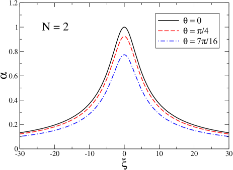
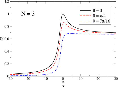
Figure 1: (Color online). Coherence visibility $\alpha$ as a function of the adimensional interaction strength $\xi=U/(2J)$ for $N=2$ (upper panel) and $N=3$ (lower panel) anyons with anyonic angle $\theta=0$ (solid line), $\theta=\pi/4$ (dashed line), and $\theta=7\pi/16$ (dot-dashed line).

A useful tool to characterize the ground state of a two-site many-body quantum system is the coherence visibility sala2011 ; minguzzi . We start considering the two site field operator ${\hat{\Psi}}(x)=\sum_{j=1,2}\Phi_{j}(x)\hat{b}_{j}$, with $\Phi_{j}(x)=\langle x|j\rangle$. Consequently the one-body density matrix, defined as $\rho_{1}(x,x^{\prime})=\langle GS|{\hat{\Psi}}^{+}(x){\hat{\Psi}}(x^{\prime})|GS\rangle$, becomes $\rho_{1}(x,x^{\prime})=\sum_{i,j=1,2}\Phi_{j}^{*}(x)\Phi_{i}(x^{\prime})\langle GS|\hat{b}_{j}^{+}\hat{b_{i}}|GS\rangle$. The momentum distribution $n(p)$, i.e. the number of particle which has momentum between $p$ and $p+dp$, could be obtained as $n(p)=\int dx\int dx^{\prime}exp[-ip(x-x^{\prime})]\rho_{1}(x,x^{\prime})$. Inserting the previous two mode ansatz, one obtain $n(p)=\sum_{i,j=1,2}\tilde{\Phi}_{j}^{*}(p)\tilde{\Phi}_{i}(p)\langle GS|{\hat{b}}_{j}^{+}\hat{b}_{i}|GS\rangle$, where the tilde means the Fourier transform of the wavefuncion. Exploiting the symmetry of the potential, and calling $d$ the distance between the minimum of the two wells, we can assume the existence of a wavefunction $\Phi(x)$ such that $\Phi_{1}(x)=\Phi(x+d/2)$ and $\Phi_{2}(x)=\Phi(x-d/2)$. Finally, defining $n_{0}(p)=N|\tilde{\Phi}(p)|^{2}$ the momentum distribution becomes

$$n(p)=n_{0}(p)\bigl{[}1+\alpha\cos({p\over\hbar}d-\delta)\bigr{]}\;,$$ (44)

where

$$\alpha=\frac{2}{N}|\gamma|$$ (45)

is the coherence visibility and

$$\gamma=\langle GS|\hat{b}_{1}^{+}\hat{b}_{2}|GS\rangle=|\gamma|\,e^{i\delta}\;$$ (46)

with $\delta$ the phase which appears in Eq. (44).

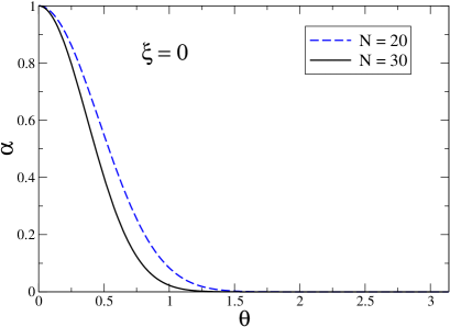
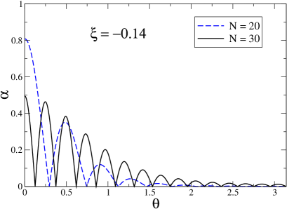
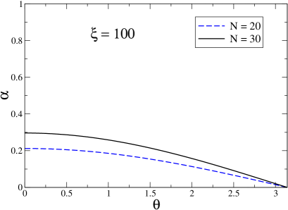
Figure 2: (Color online). Coherence visibility $\alpha$ as a function of the anyonic angle $\theta$ for three values of the adimensional interaction strength $\xi=U/(2J)$: $\xi=0$ (upper panel), $\xi=-0.14$ (middle panel), and $\xi=100$ (lower panel). In each panel there are two curves which correspond to $N=20$ (dashed line) and $N=30$ (solid line) anyons.

In Fig. 1 we report the coherence visibility $\alpha$ as a function of the adimensional interaction strength $\xi=U/(2J)$. In the upper panel we consider $2$ anyons while in the lower panel $3$ anyons. In each panel the three curves correspond to different values of the anyonic angle: solid line for $\theta=0$, dashed line for $\theta=\pi/4$, and dot-dashed line for $\theta=7\pi/16$. The figure shows that the system is maximally coherent for $\theta=0$. However, quite remarkably, the coherence visibility $\alpha$ is strongly dependent on the choice of $N$, $\theta$ and $\xi$.

In Fig. 2 we plot the coherence visibility $\alpha$ vs the anyonic angle $\theta$ for $20$ (solid line) and $30$ (dashed line) anyons. In the noninteracting case (upper panel) the decrease of $\alpha$ is very rapid approaching $\theta=\pi$ (pseudo-fermionic case) and it becomes sharper as the number of particles increases. For attractive interaction (middle panel) there are many anyonic angles for which the system is fully incoherent. Finally, in the case of strong repulsion (lower panel) the loss of coherence is less drastic and smoother by increasing the number of particles. Notice that the strength $\xi=U/(2J)$ of the attractive interaction is quite small compared to the repulsive case. This is due to the fact that in the attractive case we find numerically a rapid growth in the quasi-degeneracy between the many-body ground state and the many-body first excited state. It is important to stress that our numerical results strongly suggest that the functional dependence of the complex coefficients $c_{j}$ of Eq. (40) with respect to the anyonic angle $\theta$ is given by $c_{j}(\theta)=|c_{j}(0)|e^{i\phi_{j}(\theta)}$ with $\phi_{j}(\theta)=(j^{2}\theta/2)-j\theta(N-1/2)$ plus an arbitrary constant which does not affect the physics. This is an empirical formula, which seems to be valid for any interaction strength $\xi$ and particle number $N$.

The coherence visibility $\alpha$ of the ground state $|GS\rangle$ is strictly related to the Bose-Einstein condensate fraction $f_{0}$, which can be calculated by using the Penrose-Onsager criterion penrose . In our case $f_{0}$ is the largest eigenvalue of the $2\times 2$ one-body density matrix, whose elements are $\langle GS|{\hat{a}}_{j}^{+}{\hat{a}}_{k}|GS\rangle/N$ with $j,k=1,2$. It is then straightforward to prove (see also bruno ) that

$$f_{0}={1\over 2}\left(\alpha+1\right)\;.$$ (47)

Thus, for a full coherent ground state $|GS\rangle$, where $\alpha=1$, the condensate fraction is $f_{0}=1$. Instead for a fully incoherent ground state $|GS\rangle$, where $\alpha=0$, the condenstate fraction is $f_{0}=1/2$, which corresponds to the maximally fragmented Bose-Einstein condensate between the two sites. In Figs. 1 and 2 one can easily determine the condensate fraction $f_{0}$ of the system from the value of $\alpha$ using Eq. (47). We stress that the Penrose-Onsager definition of the condensate fraction was thought for large number of particles. In our context it is a useful tool to characterize the fragmentation of the ground state.

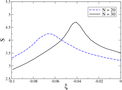
Figure 3: (Color online). Entanglement entropy $S$ as a function of the adimensional interaction strength $\xi=U/(2J)$. The two curves which correspond to $N=20$ (dashed line) and $N=30$ (solid line) anyons. As discussed in the text, $S$ does not depend on the anyonic angle $\theta$.

A relevant consequence of the fact that the transition probabilities $|c_{j}|^{2}$ of the ground state (40) do not depend on anyonic angle $\theta$ is that the entanglement entropy $S$ does not change with respect to the one calculated with $\theta=0$. In fact, the entanglement entropy

$${\color[rgb]{0,0,0}S=-\sum_{j=0}^{N}|c_{j}|^{2}\log_{2}(|c_{j}|^{2})}$$ (48)

depends on the square modulus of the coefficients $c_{i}$ and consequently their phase dependence is washed out. For the sake of completeness, in Fig. 3 we report $S$ as function of the adimensional interaction strength $\xi=U/(2J)$ for $N=20$ and $N=30$ (see also Ref. sala2011 ). In our problem, the entanglement entropy $S$ is the von Neumann entropy of the reduced matrix ${\hat{\rho}}_{j}=Tr_{k}[{\hat{\rho}}]$ of the site $j$ ($j=1$ or $j=2$), obtained performing the partial trace of the density matrix ${\hat{\rho}}=|GS\rangle\langle GS|$ of the ground state $|GS\rangle$ with respect to the states of the site $k$ ($k\neq i$). In the repulsive case ($\xi>0$) the entanglement entropy $S$ diminishes by increasing $\xi$ and $S\to 0$ when $|GS\rangle\to c_{N/2}|N/2,N/2$ for $\xi\to+\infty$, with $N$ even. Instead, in the attractive case ($\xi<0$), as shown in Fig. 3, the entanglement entropy $S$ has a maximum which depends on the particle number $N$. At the maximum, $S$ is slightly smaller that $log_{2}(N+1)$, that is the value obtained from Eq. (48) when all the probabilities $|c_{j}|^{2}$ are equal. The entanglement entropy $S\to 1$ when $|GS\rangle\to(c_{0}|0,N\rangle+c_{N}|N,0\rangle)$ for $\xi\to-\infty$, with $N$ even.

V Conclusions

We have investigated the two-site anyonic Hubbard model, which describes $N$ anyons trapped in a one-dimensional double-well potential, i.e. the anyonic version of the well-known Josephson junction. We have derived dynamical equations for the relative phase and population imbalance of the anyonic system using Jordan-Wigner transformation and coherent states. From these mean-field dynamical equations we have also shown that the choice of the anyonic angle $\theta$ is critical for the existence of stationary configurations. We have also obtained a generalized formula of the Josephson frequency, also analyzing the spontaneous symmetry breaking and the conditions for achieving the macroscopic quantum self-trapping. Finally, we have studied many-body quantum features of the exact ground state of the system. We have found that the anyonic angle has no effect on the entenglement entropy, while, on the contrary, the coherence visibility of the momentum distribution and the condensate fraction are strongly dependent on the anyonic angle. In particular, the effective statistical repulsion induced by $\theta$ reduces the coherence and the condensate fraction of the bosons. As previously stressed, our theoretical predictions could be observed if these synthetic pseudo-anyons are obtained by using one of the proposed experimental schemes roncaglia ; santos ; strater . Clearly, with only two lattice sites, particles cannot change their position, they can only hop on top of each other. However, in our configuration the connection to anyons is given by the fact that two particles can exchange their position in two ways, either picking up a phase plus theta or minus theta. From this point of view our model shows a interesting, and theoretically relevant, analogy with the braiding of two anyons in two spatial dimensions.

The authors thank Axel Pelster and Martin Bonkhoff for useful discussions and suggestions.

References

- (1) F. Wilczek, Quantum Mechanics of Fractional-Spin Particles, Phys. Rev. Lett. 49, 957 (1982).
- (2) R.B. Laughlin, Anomalous quantum Hall effect: an incompressible quantum fluid with fractionally charged excitations, Phys. Rev. Lett. 50, 1395 (1983).
- (3) B.I. Halperin, Statistics of Quasiparticles and the Hierarchy of Fractional Quantized Hall States, Phys. Rev. Lett. 52, 1583 (1984).
- (4) F.D.M. Haldane, Fractional Statistics in Arbitrary Aimensions: Generalization of the Pauli Principle, Phys. Rev. Lett. 67, 937 (1991).
- (5) G. Gentile, Osservazioni sopra le statistiche intermedie, Nuovo Cimento 17, 493 (1940).
- (6) Y.-J. Lin, K. Jimenez-Garcia, and I.B. Spielman, A spin-orbit coupled Bose-Einstein condensate, Nature 471, 83 (2011).
- (7) V. Galitski and I.B. Spielman, Spin-orbit coupling in quantum gases, Nature 494, 49 (2013).
- (8) T. Keilmann, I. McCulloch, and M. Roncaglia, Statistically induced phase transitions and anyons in 1D optical lattices, Nature Commun. 2, 361 (2011).
- (9) S. Greschner and L. Santos, Anyon Hubbard Model in One-Dimensional Optical Lattices, Phys. Rev. Lett. 115, 053002 (2015).
- (10) C. Strater, S.C.L. Srivastava, and A. Eckard, Floquet realization and signatures of one-dimensional anyons in a optical lattice, Phys. Rev. Lett. 117, 205303 (2016).
- (11) G. Tang, S. Eggert, and A. Pelster, Ground-state properties of anyons in a one-dimensional lattice, New J. Phys. 17, 123016 (2015).
- (12) W. Zhang, S. Greschner, E. Fan, T.C. Scott, and Y. Zhang, Ground-state properties of the one-dimensional unconstrained pseudo-anyon Hubbard model, Phys. Rev. A 95, 053614 (2017).
- (13) M. Lewenstein, A. Sanpera, and V. Ahufinger, Ultracold Atoms in Optical Lattices: Simulating Quantum Many-Body Systems (Oxford Univ. Press, 2012).
- (14) M. Bonkhoff, K. Jägering, S. Eggert, A. Pelster, M. Thorwart, and T. Posske, Bosonic Continuum Theory of One-Dimensional Lattice Anyons, Phys. Rev. Lett. 126, 163201 (2021).
- (15) B. D. Josephson, Possible new effects in superconductive tunnelling, Phys. Lett. 1, 251 (1962).
- (16) A. Barone and G. Paterno, Physics and Applications of the Josephson effect (Wiley, New York, 1982).
- (17) E. L. Wolf, G.B. Arnold, M.A. Gurvitch, and John F. Zasadzinski, Josephson Junctions: History, Devices, and Applications (Pan Stanford Publishing, Singapore, 2017).
- (18) A. Smerzi, S. Fantoni, S. Giovanazzi, and S.R. Shenoy, Quantum Coherent Atomic Tunneling between Two Trapped Bose-Einstein Condensates, Phys. Rev. Lett. 79, 4950 (1997).
- (19) M. Albiez, R. Gati, J. Fölling, S. Hunsmann, M. Cristiani, and M.K. Oberthaler, Direct Observation of Tunneling and Nonlinear Self-Trapping in a Single Bosonic Josephson Junction, Phys. Rev. Lett. 95, 010402 (2005).
- (20) S. Wimberger, G. Manganelli, A. Brollo, and L. Salasnich, Finite-size effects in a bosonic Josephson junction, Phys. Rev. A 103, 023326 (2021).
- (21) G. Mazzarella, L. Salasnich, A. Parola, and F. Toigo, Coherence and entanglement in the ground state of a bosonic Josephson junction: From macroscopic Schrödinger cat states to separable Fock states, Phys. Rev. A 83, 053607 (2011).
- (22) G. Ferrini, A. Minguzzi and F.W.J. Hekking, Number squeezing, quantum fluctuations, and oscillations in mesoscopic Bose Josephson junctions, Phys. Rev. A 78, 023606 (2008).
- (23) A. Escriva, A. Richaud, B. Julia-Diaz, and M. Guilleumas, Static properties of two linearly coupled discrete circuits, J. Phys. B: At. Mol. Opt. Phys. 54, 115301 (2021).
- (24) W. E. Arnoldi, The principle of minimized iterations in the solution of the matrix eigenvalue problem, Quarterly Appl. Math. 9, 17 (1951).
- (25) S. Wolfram, The Mathematica Book (Wolfram Media, 2003).
- (26) O. Penrose and L. Onsager, Bose-Einstein condensation and liquid helium, Phys. Rev. 104, 576 (1956).