DoF-NeRF: Depth-of-Field Meets Neural Radiance Fields

Abstract.

Neural Radiance Field (NeRF) and its variants have exhibited great success on representing 3D scenes and synthesizing photo-realistic novel views. However, they are generally based on the pinhole camera model and assume all-in-focus inputs. This limits their applicability as images captured from the real world often have finite depth-of-field (DoF). To mitigate this issue, we introduce DoF-NeRF, a novel neural rendering approach that can deal with shallow DoF inputs and can simulate DoF effect. In particular, it extends NeRF to simulate the aperture of lens following the principles of geometric optics. Such a physical guarantee allows DoF-NeRF to operate views with different focus configurations. Benefiting from explicit aperture modeling, DoF-NeRF also enables direct manipulation of DoF effect by adjusting virtual aperture and focus parameters. It is plug-and-play and can be inserted into NeRF-based frameworks. Experiments on synthetic and real-world datasets show that, DoF-NeRF not only performs comparably with NeRF in the all-in-focus setting, but also can synthesize all-in-focus novel views conditioned on shallow DoF inputs. An interesting application of DoF-NeRF to DoF rendering is also demonstrated. The source code will be made available at https://github.com/zijinwuzijin/DoF-NeRF.

Figure 1. Given a set of shallow depth-of-field (DoF) images, (c) performance of NeRF deteriorates due to its (a) pinhole camera model assumption. We present DoF-NeRF, a novel NeRF-based framework using (b) explicit DoF simulation to represent (d) all-in-focus scenes from shallow DoF inputs. An application of DoF-NeRF to (e) DoF rendering is also presented.

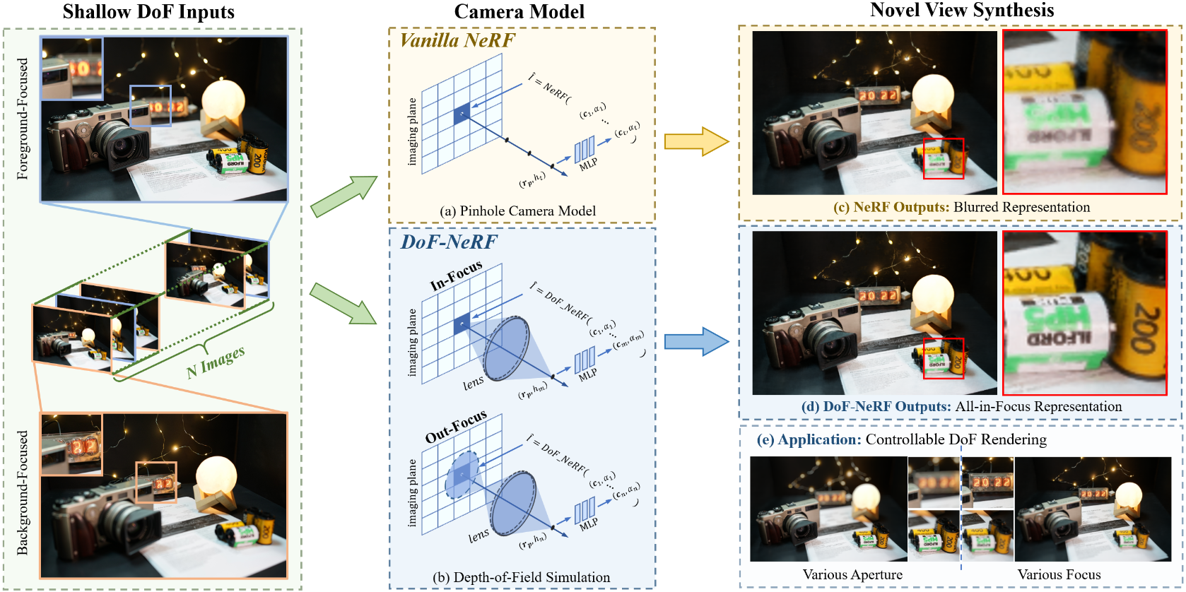
Fig 1

1. Introduction

Novel view synthesis (Debevec et al., 1996; Gortler et al., 1996; Levoy and Hanrahan, 1996) is a long-standing problem in computer vision and graphics. As synthesizing novel views of a 3D scene from a sparse set of input images is a fundamental task for applications in augmented reality (AR) and virtual reality (VR), a substantial amount of work has been conducted to seek for solutions. Recently Neural Radiance Field (NeRF) (Mildenhall et al., 2020), an implicit multi-layer perceptron (MLP) based model that regresses colors and densities from 3D coordinates and 2D viewing directions, shows an impressive level of fidelity on novel view synthesis. In particular, NeRF uses classical volume rendering techniques (Kajiya and Von Herzen, 1984) to synthesize photo-realistic novel views by integrating the output colors and densities along emitted rays. Since the process of volume rendering is fully differentiable, NeRF can be optimized by minimizing the difference between the captured images and the rendered views.

However, NeRF and its variants (Martin-Brualla et al., 2021; Zhang et al., 2020; Deng et al., 2022) are generally based on the pinhole camera model and assume all-in-focus inputs, i.e., both foreground and background are clear. In reality, images captured from the real world often have finite depth-of-field (DoF). Namely, points of light that do not lie on the focal plane are imaged to a circular region on the sensor plane, rather than to single points. The size of the circular region (dubbed circle of confusion, or CoC) is affected by the diameter of the aperture (aperture size) and the distance from the camera to the focal plane (focus distance). Hence, photos captured with a small aperture usually present wide DoF, i.e., all objects are clear. In contrast, as the aperture diameter increases, objects that near the focal plane remain clear, but those far from the plane are blurred with a large CoC. This shallow DoF effect is ubiquitous in photography especially when shooting with a wide-aperture lens or taking close-up photos.

While NeRF has shown astonishing results for novel view synthesis, its performance deteriorates when processing shallow DoF inputs. This can boil down to the assumption of the pinhole camera model—when predicting pixel colors, NeRF only considers the emission of spatial points on the ray passing through the pixel and neglects the scattered radiance from neighboring rays. To resolve this issue, we present DoF-NeRF, a novel NeRF-based framework that enables NeRF to tackle shallow DoF inputs. Specifically, we introduce three key changes: (1) a differentiable representation of CoC to simulate the radiance scattered between rays; (2) learnable parameters to enable direct manipulation of the DoF effect; (3) a patch-based ray selecting method for efficient optimization. Our key insight is to simulate the DoF effect by an optical-conforming radiance scattering method parameterized with two learnable parameters: aperture size and focus distance. The two parameters of each training view can guide the optimization of NeRF to generate a clear 3D scene representation. Our optical modeling of DoF can not only synthesize all-in-focus novel views conditioned on shallow DoF inputs, but also provide highly controllable DoF rendering from novel viewpoints. Our main contributions include the following.

• We present DoF-NeRF, a novel neural rendering framework that can represent clear 3D scenes given shallow DoF inputs.

• We introduce the Concentrate-and-Scatter technique, a plug-and-play rendering modification for NeRF-based methods to simulate the DoF effect.

• We also contribute a new dataset for novel view synthesis of shallow DoF scenes. This dataset contains triplets of all-in-focus, foreground-focused, and background-focused from sparse viewpoints for each scene. Both real-world and synthetic data are included for further study.

Figure 2. Basic principle of DoF-NeRF. The vanilla NeRF (a) adopts a pinhole camera model which ignores the DoF effect. DoF-NeRF computes the observed color of ray $\bm{r}_{\bm{p}}$ by adding (b) color diffusion $\hat{I}_{ray}(\bm{p})$: the predicted radiance of spatial points on ray $\bm{r}_{\bm{p}}$ is diffused to a CoC on the imaging plane, and (c) radiance scattering $\hat{I}_{scatter}(\bm{p})$: the scattered radiance of spatial points on neighboring rays, e.g., $\bm{r}_{\bm{p}_{1}},\bm{r}_{\bm{p}_{2}}$ may affect the observed color of $\bm{r}_{\bm{p}}$. An indicator function is used to distinguish points by the CoC diameter and the distance to ray $\bm{r}_{\bm{p}}$. The observed color of ray $\bm{r}_{\bm{p}}$ is the combination of $\hat{I}_{ray}(\bm{p})$ and $\hat{I}_{scatter}(\bm{p})$.

Illus. of DoF-NeRF pipeline

2. Related Work

2.1. Novel View Synthesis

Novel view synthesis is a task of synthesizing novel camera perspectives from a set of input views and their corresponding camera poses. The research into novel view synthesis has a long history in computer vision and graphics community. Various approaches are investigated, including image-based rendering (Debevec et al., 1996; Gortler et al., 1996; Levoy and Hanrahan, 1996) and explicit geometric representations such as voxel grids (Liao et al., 2018; Jimenez Rezende et al., 2016; Xie et al., 2019), point clouds (Achlioptas et al., 2018; Fan et al., 2017), triangle meshes (Kanazawa et al., 2018; Ranjan et al., 2018; Wang et al., 2018), and multiplane images (MPIs) (Zhou et al., 2018; Flynn et al., 2019; Tucker and Snavely, 2020). Recent studies (Sitzmann et al., 2019b; Mildenhall et al., 2019; Sitzmann et al., 2019a; Lombardi et al., 2019) have shown the superiority of implicit representations in rendering high quality novel views. For example, Mildenhall et al. propose Neural Radiance Field (NeRF) (Mildenhall et al., 2020), an implicit MLP-based model that maps 3D coordinates plus 2D viewing directions to opacity and color values, which is capable of representing a complex 3D scene and rendering photo-realistic novel views.

However, drawbacks of NeRF remain, including entailing immense posed images and its high computational requirements for rendering novel views. To mitigate these issues, researchers have introduced improvements upon NeRF to extend its performance and applicability, such as faster training (Deng et al., 2022; Sun et al., 2022), faster inference (Reiser et al., 2021; Garbin et al., 2021), optimizing NeRF with low-light (Mildenhall et al., 2022) or high dynamic range (Huang et al., 2022) images, improving generalization (Schwarz et al., 2020; Niemeyer and Geiger, 2021), and representing dynamic scenes (Li et al., 2021; Xian et al., 2021a). Recently, Self-Calibrating NeRF (Jeong et al., 2021) combines the pinhole camera, radial distortion, and a generic non-linear camera distortion for self-calibration by modeling distortion parameters. However, all these methods neglect the DoF effect. In this paper, we extend NeRF to simulate the aperture of lens and model the DoF effect by optimizing two learnable parameters, i.e., aperture size and focus distance. This enables the synthesis of all-in-focus novel views with shallow DoF inputs as well as the rendering of 3D scenes with arbitrary aperture and focus distance settings.

2.2. DoF Rendering

Rendering DoF effects from a single all-in-focus image has been well studied in previous work. Some work (Dutta et al., 2021; Ignatov et al., 2019, 2020b, 2020a; Qian et al., 2020) directly regresses a shallow DoF image using neural networks. However, these methods cannot adjust DoF effects as they are trained on EBB! dataset (Ignatov et al., 2020a) which only provides pairs of wide and shallow DoF images. The DoF effects in (Busam et al., 2019; Peng et al., 2021; Wadhwa et al., 2018; Xian et al., 2021b; Xiao et al., 2018; Zhang et al., 2019) are controllable but usually require an extra disparity map. Although the disparity map can be predicted by depth estimation, its accuracy is not guaranteed. Another challenge is the revealing of invisible background objects during rendering, because no image of other views is provided.

To address these problems, several methods focusing on synthesizing DoF effects on NeRF models have been proposed recently. RawNeRF (Mildenhall et al., 2022) adopts a multi-plane representation to render DoF effects, while NeRFocus (Wang et al., 2022) proposes a frustum-based volume rendering to approximate the imaging of a thin lens model. However, both studies mentioned above still assume all-in-focus inputs. In this work, through appropriate optical modeling, we optimize the aperture diameters and the focus distances during training and render clear novel views with shallow DoF inputs.

3. Preliminary

In this section, we briefly review the principle of NeRF. To represent a scene, NeRF optimizes a continuous function parameterized by an MLP network $G_{\Theta}:(\bm{x},\bm{d})\rightarrow(\bm{c},\alpha)$ which maps a spatial position $\bm{x}=(x,y,z)$ and viewing direction $\bm{d}=(\theta,\varphi)$ to its corresponding emitted color $\bm{c}$ and transparency $\alpha$. the observed color $\hat{I}_{n}(\bm{p})$ of the pixel $\bm{p}$ can be represented as an integral of all emitted colors weighted by the opaqueness along the camera ray $\bm{r}_{\bm{p}}(h)$, or can be written as the weighted radiance at $N_{s}$ sample points along a ray:

(1) $$\hat{I}_{n}(\bm{p})=\sum_{i=1}^{N_{s}}T_{i}(1-\alpha(\bm{r}_{\bm{p}}(h_{i}),\Delta_{i}))\bm{c}(\bm{r}_{\bm{p}}(h_{i}),\bm{d})\,,$$

where $\Delta_{i}=h_{i+1}-h_{i}$ and

(2) $$T_{i}=\prod_{j=1}^{i-1}\alpha(\bm{r}_{\bm{p}}(h_{j}),\Delta_{j})$$

denotes the accumulated transmittance along the ray, i.e., the probability of the emitted light travelling from $h_{1}$ to $h_{i}$ without hitting other particles. Computing the color value of each pixel on the imaging plane via volume rendering above composites a complete image.

To optimize the continuous function $G_{\Theta}$ from a set of input images $\mathcal{I}=\{I_{1},I_{2},...I_{N}\}$, NeRF adopts the photometric error between the synthesized views $\hat{\mathcal{I}}$ and corresponding observations $\mathcal{I}$:

(3) $$\mathcal{L}=\sum_{n=1}^{N}\|I_{n}-\hat{I}_{n}\|_{2}^{2}\,.$$

Note that, vanilla NeRF assumes a linear pinhole camera model where the color value of a pixel $\bm{p}=(u,v)$ on the imaging plane is only determined by a single camera ray $\bm{r}(h)=\bm{o}+h\bm{d}$ that travels from the camera center $\bm{o}$ and passes through the pixel $\bm{p}$ along the viewing direction $\bm{d}$. Therefore, NeRF ignores the interference between rays and does not model the aperture structure, leading to its incapability to simulate the DoF effect.

4. Approach

Instead of assuming the linear pinhole camera model in volume rendering, we extend NeRF to incorporate the representation of CoC to simulate the DoF. This allows NeRF to approximate the DoF effect under arbitrary aperture size and focus distance configuration such that all-in-focus scenes can be represented with shallow DoF inputs.

The emergence of DoF consists of two steps: radiance of the spatial points scattering to a particular area and center ray accepting the scattered radiance from neighboring rays. We implement these two steps by combining optical models and classical volume rendering (Fig. 2). To optimize NeRF with shallow DoF images, we introduce two learnable parameters: the aperture parameters $\mathcal{K}=\{K_{1},K_{2},...K_{N}\}$ and the focus distances $\mathcal{F}=\{F_{1},F_{2},...F_{N}\}$ for $N$ images in the training set $\mathcal{I}$. The aperture parameters and focus distances are jointly optimized in the training process.

In what follows, we first introduce our explicit aperture modeling and then explain how DoF-NeRF is optimized. The table of notations can be found in the appendix.

4.1. DoF in Radiance Field

The physical model of imaging and DoF has been well studied in geometric optics (Hecht, 2017; Li et al., 2005). Assume that we neglect the ray distortions caused by the lens. In an ideal optical system, a spatial point $\bm{p}$ with the point-to-lens distance (object distance) $h_{t}$ is projected to a circular region (CoC) on the imaging plane. The diameter of the region $\delta(h_{t})$ can be determined by the focal length $f$, aperture diameter $D$, and focus distance $F$, which amounts to the following equation

(4) $$\delta(h_{t})=fD\times\frac{\left|h_{t}-F\right|}{h_{t}(F-f)}\,.$$

Since the focus distance $F$ and object distance $h_{t}$ are often much larger than the focal length $f$, we can modify Eq. (4) such that

(5) $$\delta(h_{t})=fD\times\frac{\left|h_{t}-F\right|}{Fh_{t}}=fD\times\left|\frac{1}{F}-\frac{1}{h_{t}}\right|=K\times\left|\frac{1}{F}-\frac{1}{h_{t}}\right|\,,$$

where the product of focal length and aperture diameter can be replaced by an aperture parameter $K=f\times D$.

For simplicity, we assume that the emitted radiance $\hat{C}(\bm{p},h_{t})$ of the spatial point evenly disperses to a CoC of diameter $\delta(h_{t})$:

(6) $$\hat{C}(\bm{p},h_{t})=\frac{\left(1-\alpha\left(\bm{r}_{\bm{p}}(h_{t}),\Delta_{t}\right)\right)\bm{c}\left(\bm{r}_{\bm{p}}(h_{t}),\bm{d}\right)}{S(h_{t})}\,,$$

where $S(h_{t})=\pi\delta^{2}(h_{t})/4$ denotes the area of the CoC.

Different from the pinhole camera assumption, the observed color of the ray $\bm{r}_{\bm{p}}$ can also be affected by spatial points whose CoC radius is larger than the distance to the ray $\bm{r}_{\bm{p}}$. Apparently, points on neighboring rays only contribute to the radiance accumulation without affecting the transmittance $T(\bm{r}_{\bm{p}})$. Given $M$ rays specific to pixels $\bm{\mathcal{P}}=\{\bm{p}_{1},\bm{p}_{2},...,\bm{p}_{M}\}$ on which the scattered radiance of spatial points may affect the color prediction of center ray $\bm{r}_{\bm{p}}$, we can compute the color $\hat{I}$ of pixel $\bm{p}$ by summing up emitted radiance. without changing the transmittance coefficient. Specifically, computing the observed color $\hat{I}(\bm{p})$ can be split into two parts: $\hat{I}_{ray}(\bm{p})$ and $\hat{I}_{scatter}(\bm{p})$ which respectively represent the diffused radiance on ray $\bm{r}_{\bm{p}}$ and the scattered radiance from other rays. This takes the form

(7) $$\hat{I}_{ray}(\bm{p})=\sum_{i=1}^{N_{s}}T_{i}\hat{C}(\bm{p},h_{i})\,,$$

(8) $$\hat{I}_{scatter}(\bm{p})=\sum_{j=1}^{M}\sum_{i=1}^{N_{s}}\mathds{1}_{\delta(h^{\prime}_{i})>2\|\bm{p}-\bm{p}_{j}\|_{2}^{2}}T^{\prime}_{ij}\hat{C}(\bm{p}_{j},h^{\prime}_{i})\,,$$

(9) $$\hat{I}(\bm{p})=\hat{I}_{ray}(\bm{p})+\hat{I}_{scatter}(\bm{p})\,,$$

where $h_{i}$ and $h^{\prime}_{i}$ denote the depth of the $i$-th sample point on the center ray and neighboring rays, respectively; $T_{i}$ denotes the accumulated transmittance of the $i$-th sample point on the ray $\bm{r}_{\bm{p}}$ , and $T^{\prime}_{ij}$ denotes the transmittance of scattered radiance from the $i$-th sample point on the ray specific to pixel $\bm{p}_{j}$. An indicator function $\mathds{1}$ is used to distinguish points by the CoC diameter $\delta(h^{\prime}_{i})$ and the distance to ray $\bm{r}_{\bm{p}}$.

Figure 3. Visualization of volume coefficients $K_{volume}$. In (a), we randomly choose $3$ rays from the 3D scene and visualize the volume coefficient $K_{volume}$ of sample points on each ray according to the depth. Different colors in (a) denote different rays. In (b) the histogram shows the value distribution of $K_{volume}$ of $1024$ selected rays, and the polyline shows the accumulated $K_{volume}$ of points in each bin of the histogram.

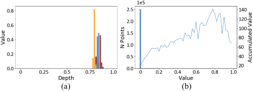
vis. of K_volume

However, computing the color of the ray $\bm{r}_{\bm{p}}$ directly following Eq. (6)$\sim$(9) can be rather inefficient. It requires traversing all the spatial points on neighboring rays to obtain the color of the center rays.

To mitigate this issue, we analyze a fact of the volume rendering and propose our solution in what follows. For spatial points on the ray $\bm{r}_{\bm{p}}$, we evaluate their contributions to the color prediction with a volume rendering coefficient $K_{volume}$:

(10) $$K_{volume}(\bm{r}_{\bm{p}},h_{t})=T_{t}\left(1-\alpha\left(\bm{r}_{\bm{p}}(h_{t}),\Delta_{t}\right)\right)\,.$$

We randomly choose $1024$ rays from input views and visualize the distribution of the volume coefficients (see Fig. 3). For most rays, points with large volume coefficients gather in a narrow depth interval. The distribution of the volume coefficient indicates that most spatial points do not affect the observed color but incur considerable computational overhead.

Figure 4. Illustration of our concentrate-and-scatter rendering. To reduce the cost of computation, we first concentrate the emitted radiance of points on the ray $\bm{r}_{\bm{p}}$ (right side of the imaging plane) to the concentration depth $h_{c}$ (orange point) and calculate the corresponding CoC diameter. Then we scatter the concentrated radiance to the neighboring areas within its CoC diameter (left side of the imaging plane).

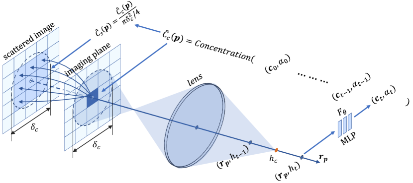
Illus. of con-n-scat method

Nonetheless, simply ignoring those points may lead to the brightness change of rendered images. In the view of the volume coefficients distribution, we introduce the idea of concentrate-and-scatter rendering. As shown in Fig. 4, the core idea is to concentrate the emitted radiance of all the spatial points along the ray to the concentration depth $h_{c}$, and to scatter the concentrated radiance to its corresponding CoC. Since the scattered radiance does not affect the transmittance on the ray $\bm{r}_{\bm{p}}$, the concentration of the radiance follows the original volume rendering. For $N_{s}$ sampled points along the ray $\bm{r}_{\bm{p}}$, the concentration depth $h_{c}$, CoC diameter $\delta_{c}$ of the concentration point, and the scattered radiance $\hat{C}_{s}(\bm{p})$ can be formulated by

(11) $$h_{c}(\bm{p})=\frac{\sum_{i=1}^{N_{s}}K_{volume}(\bm{r}_{\bm{p}},h_{t})h_{i}}{\sum_{i=1}^{N_{s}}K_{volume}(\bm{r}_{\bm{p}},h_{t})}\,,$$

(12) $$\delta_{c}(\bm{p})=K\left|\frac{1}{F}-\frac{1}{h_{c}}\right|\,,$$

(13) $$\hat{C}_{s}(\bm{p})=\frac{\sum_{i=1}^{N_{s}}K_{volume}(\bm{r}_{\bm{p}},h_{t})\bm{c}(\bm{r}_{\bm{p}}(h_{i}),\bm{d})}{\pi\delta_{c}^{2}(\bm{p})/4}\,.$$

For $P$ rays with respect to the pixels $\bm{\mathcal{P}}=\{\bm{p}_{1},\bm{p}_{2},...\bm{p}_{P}\}$ whose radiance may affect the color prediction of ray $\bm{r}_{\bm{p}}$, including the ray $\bm{r}_{\bm{p}}$ itself, the observed color of ray $\bm{r}_{\bm{p}}$ can be defined by

(14) $$\hat{I}(\bm{p})=\sum_{j=1}^{P}\mathds{1}_{\delta_{c}(\bm{p})>2\|\bm{p}-\bm{p}_{j}\|_{2}^{2}}\hat{C}_{s}(\bm{p}_{j})\,.$$

We implement the algorithm with the CuPy package to achieve a significant speedup. The detail of the algorithm can be found in the appendix.

4.2. Ray Selection

When optimizing the scene representation, vanilla NeRF randomly chooses $N_{rand}$ rays from all input views. Since the simulation of the DoF effect requires to consider radiance scattered from neighboring rays, a straight-forward approach is to compute several rays that may affect the center ray. This method is of low efficiency in training as it only considers the observed color of the center ray in a single iteration. Yet another approach is to compute the concentrated radiance of all rays from one imaging plane and to scatter every pixels on the whole imaging plane. However, it entails to compute every ray of the whole imaging plane in each iteration, which leads to an unacceptable cost in computing.

Figure 5. Illustration of our patch-based optimization. Instead of randomly choosing rays (a) as in NeRF, we optimize DoF-NeRF by selecting rays from a concentrated area in each iteration (b).

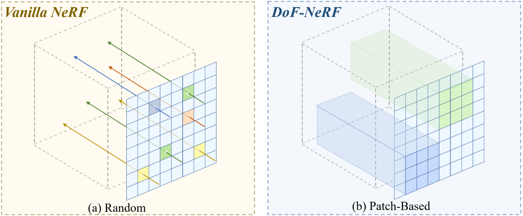
Illus. of con-n-scat method

We adopt a patch-based ray selection method (Fig. 5) which can be considered as a compromise between the two approaches above. We construct a group of anchors, where each anchor is set every $N_{anchor}$ pixels on the imaging plane of inputs and determines the center of an $N_{patch}\times N_{patch}$ patch. In each iteration, we randomly choose one patch and guide rays passing though pixels in the selected patch. Observed colors of the pixels are computed using the concentrate-and-scatter rendering mentioned above.

Input: $N$ images $\mathcal{I}=\{I\}_{i=1}^{N}$

Output: NeRF Model $G_{\Theta}$, aperture $[\hat{K}]_{i=1}^{N}$, focus distance $[\hat{F}]_{i=1}^{N}$

1 import torch.nn as nn

2 $[\hat{K}]$ = nn.Parameter(shape=(N, 1), requires_grad=True)

3 $[\hat{F}]$ = nn.Parameter(shape=(N, 1), requires_grad=True)

4 $G_{\Theta}$ = NeRF_Model(requires_grad=True)

5 for i in range($N_{iters}$) do

6       if $i<N_{pretrain}$ then

7             $[\bm{r}]_{i},I_{i}$=random_rays($\mathcal{I}$)

8             $\hat{I}_{i}$=Volume_Rendering($G_{\Theta},[\bm{r}]_{i}$) # Sec. 3

9             $\mathcal{L}$=loss($\hat{I}_{i},I_{i}$) # Eq. 3

10             $\mathcal{L}$.backward( )

11             optimizer.update($\hat{\Theta}$)

12            

13      else

14             $[\bm{r}]_{i},I_{i}$=patch_rays($\mathcal{I}$) # Sec. 4.2

15             $[\hat{\bm{C}}]_{i},[h_{c}]_{i}$=Concentration($G_{\Theta},[\bm{r}]_{i}$) # Eq. 13

16             $[\delta_{c}]_{i}$=CoC_Radius($[h_{c}],\hat{K}_{i},\hat{F}_{i}$) # Eq. 12

17             $\hat{I}_{i}$=Scatter($[\hat{\bm{C}}]_{i},[\delta_{c}]_{i}$) # Eq. 14

18             $\mathcal{L}$=loss($\hat{I}_{i},I_{i}$) # Eq. 3

19             $\mathcal{L}$.backward( )

20             optimizer.update($\hat{\Theta},[\hat{K}],[\hat{F}]$)

21            

22       end if

23      

24 end for

25

Algorithm 1 Joint Optimization of DoF-NeRF

4.3. Joint Optimization

Although using randomly chosen rays in the simulation of DoF effect is unpractical, it shows high efficiency in optimizing the geometric representation of 3D scenes. The patch-based method, however, often leads to divergence or sub-optimal results due to the gathering of rays. Thus, we resort to a two-stage optimization process to reduce the complexity of learning geometry representation, aperture size, and focus distance.

At the first stage, we train the NeRF network with the aperture parameter set to $0$, which degenerates the rendering model to a linear pinhole camera. In this stage, the aperture parameters and focus distances are not optimized, and the classical ray-choosing and volume rendering are adopted. This stage aims to generate a coarse 3D representation where the rendered foreground and background may be blurred due to the shallow DoF inputs. At the second stage, we further optimize the NeRF network with the concentrate-and-scatter method using patch-based ray selection. The aperture parameters, focus distances, and the NeRF network parameters are jointly optimized. We summarize our learning algorithm in Algorithm 1.

Figure 6. Comparison of NeRF and our approach in all-in-focus rendering with shallow DoF inputs. The first and third column shows the images rendered by NeRF and our approach, respectively. PSNR is shown at the upper left corner. We zoom in all the yellow boxes in the second and fourth column with error maps ($0$ to $0.1$ pixel intensity range) shown at the lower right corner. The first two rows show the result of scenes from the synthetic dataset, and the third and fourth rows are scenes from the real-world dataset.

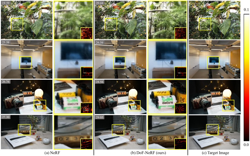
Visualization of main exp in synthetic dataset.

Table 1. Comparison of NeRF (Mildenhall et al., 2020) and our framework in the real-world dataset.

Scene	Model	PSNR$(\uparrow)$	SSIM$(\uparrow)$	LPIPS$(\downarrow)$
amiya	NeRF	26.924	0.9092	0.1633
	ours	28.311	0.9289	0.1370
camera	NeRF	25.593	0.8862	0.1574
	ours	27.714	0.9134	0.1259
plant	NeRF	28.272	0.8961	0.1581
	ours	30.317	0.9290	0.1178
turtle	NeRF	33.531	0.9566	0.0939
	ours	34.965	0.9647	0.0823

5. Results and Discussions

5.1. Dataset and Evaluation

We evaluate our method on both a real-world dataset and a synthetic dataset. The real-world dataset consists of $7$ scenes, where each contains $20\sim 30$ image triplets. Each triplet includes an all-in-focus image taken with small aperture and two images taken with large aperture focusing on the foreground and background, respectively. We generate camera parameters by COLMAP (Schonberger and Frahm, 2016) using all-in-focus images. The synthetic dataset is generated based on depth estimation and a recent single-image DoF rendering framework: for each image in the Real Forward-Facing dataset (Mildenhall et al., 2020), we use DPT (Ranftl et al., 2021) to generate the disparity map and BokehMe (Peng et al., 2022) to render shallow DoF images. Details of the datasets can be found in the appendix.

Table 2. Comparison of NeRF (Mildenhall et al., 2020) and our framework in the synthetic dataset.

Scene	Model	PSNR $(\uparrow)$	SSIM$(\uparrow)$	LPIPS$(\downarrow)$
fortress	NeRF	28.142	0.7826	0.2011
	ours	29.168	0.8099	0.1830
leaves	NeRF	19.450	0.6541	0.3190
	ours	20.025	0.7000	0.2766
room	NeRF	26.668	0.8743	0.1961
	ours	29.443	0.9135	0.1502
trex	NeRF	24.433	0.8379	0.1723
	ours	25.726	0.8744	0.1564

Figure 7. Comparison of DS-NeRF (Deng et al., 2022) and our approach in the synthetic dataset. For each scene, the zoom-in of rendered images and error maps ($0$ to $0.2$ pixel intensity range) are presented. They are respectively obtained from DS-NeRF (first row) and our model (second row). For each subfigure, PSNR is shown on the lower left.

Visualization of main exp in synthetic dataset.

Following (Mildenhall et al., 2020), we adopt PSNR, SSIM (Wang et al., 2004) and LPIPS (Zhang et al., 2018) as evaluation metrics. In all the experiments, all images are of $497\times 331$ resolution for the real-world dataset and $504\times 378$ for the synthetic dataset. $1/9$ of the images are held out for testing. $50\%$ foreground-focused images and $50\%$ background-focused images make up the training images. Both our method and vanilla NeRF adopt the same mixing order of images in each scene.

5.2. Improvement over Vanilla NeRF

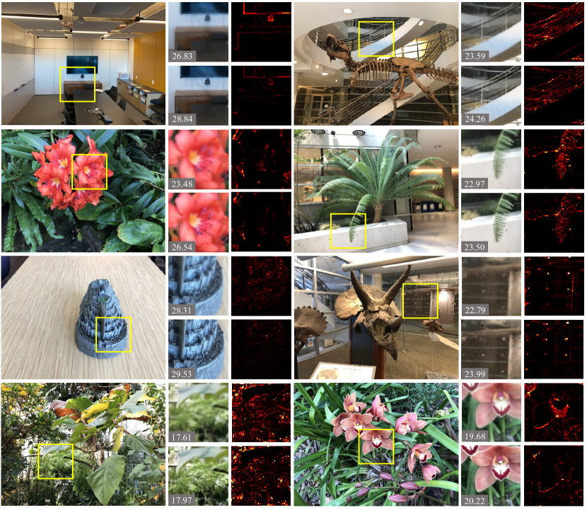
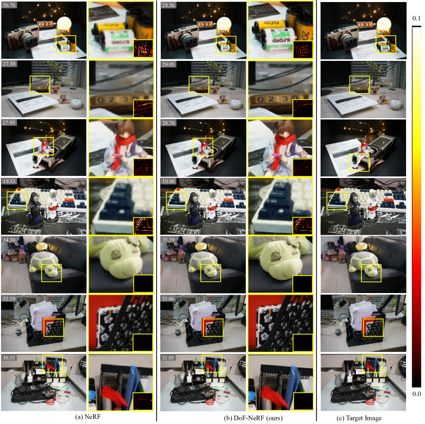
In this section, we compare DoF-NeRF qualitatively and quantitatively with vanilla NeRF on the real-world and synthetic datasets. We set the aperture parameters of the DoF-NeRF to zero and render all-in-focus novel views for evaluation. As shown in Table 1 and Table 2, one can observe that our method demonstrates better perceptual qualities than vanilla NeRF when rendering all-in-focus novel views on both two datasets. This implies that our explicit aperture modeling enables NeRF to tackle shallow DoF inputs and benefits all-in-focus novel view synthesis. We also provide the qualitative comparisons in Fig. 6. As can be seen, vanilla NeRF is prone to generate blurry renderings and miss some texture details. In contrast, our DoF-NeRF can synthesize photo-realistic all-in-focus novel views with fine-grained details.

5.3. Improvement over DS-NeRF

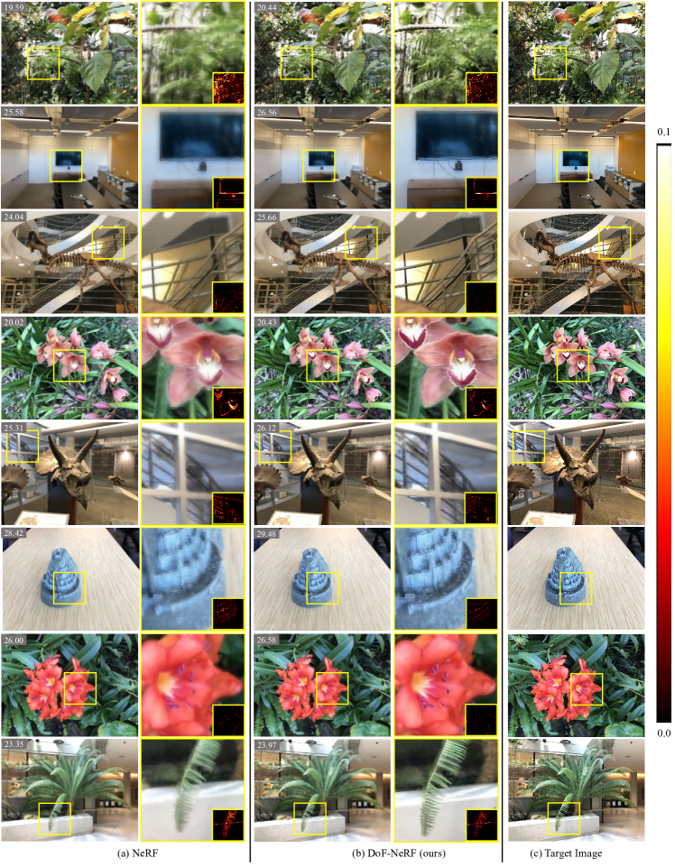
Since our DoF-NeRF is a modification of volume rendering, it can work on variants of NeRF as a plug-and-play module. To show this, we substitute the NeRF architecture with DS-NeRF (Deng et al., 2022) and use the same optimization technique. We then compare DS-NeRF and our model in the synthetic dataset. As shown in Table 3, the inclusion of our DoF module results in better rendering quality with shallow DoF images as inputs. The qualitative results are visualized in Fig. 7.

5.4. Comparison on All-in-Focus Inputs

Here we present the comparison on the all-in-focus dataset. To additionally validate the effectiveness of our method in the all-in-focus setting, we design an experiment where wide DoF images from the Real Forward-Facing dataset (Mildenhall et al., 2020) are used as inputs and adopt the same initialization, training, and rendering settings as the experiments conducted on the shallow DoF data. Table 4 reports the quantitative comparison on the all-in-focus dataset. Although our framework is originally designed for shallow DoF inputs, experiments indicate that it shows comparable performance against vanilla NeRF using all-in-focus images as inputs.

Table 3. Comparison of DS-NeRF (Deng et al., 2022) and our framework in the synthetic dataset.

Scene	Model	PSNR$(\uparrow)$	SSIM$(\uparrow)$	LPIPS$(\downarrow)$
fortress	DS-NeRF	28.493	0.7609	0.2373
	ours	29.704	0.8112	0.1970
leaves	DS-NeRF	17.872	0.5096	0.4358
	ours	18.312	0.5689	0.3840
room	DS-NeRF	26.8301	0.8641	0.2287
	ours	29.550	0.9045	0.1817
trex	DS-NeRF	22.334	0.7063	0.3438
	ours	23.600	0.7764	0.2773

Table 4. Comparison of NeRF (Mildenhall et al., 2020) and our framework in the all-in-focus dataset.

Scene	Model	PSNR$(\uparrow)$	SSIM$(\uparrow)$	LPIPS$(\downarrow)$
fortress	NeRF	33.973	0.9411	0.0469
	ours	34.007	0.9422	0.0454
leaves	NeRF	21.586	0.7854	0.1629
	ours	21.487	0.7861	0.1599
room	NeRF	33.852	0.9593	0.0721
	ours	33.760	0.9584	0.0735
trex	NeRF	30.287	0.9501	0.0601
	ours	30.222	0.9499	0.0605

5.5. DoF Rendering

Figure 8. Visualization of adjustable DoF rendering. Apart from (a) all-in-focus rendering, we can manipulate DoF effect by changing aperture and focus settings. We set $F$ to $2.0$ and $K$ to (b) $8$ and (c) $15$ respectively to render images with various aperture parameters. By holding $K$ at $15$, we change $F$ to (d) $5.0$ to create images with different focus distance.

Rendering various views.

Apart from representing all-in-focus 3D scenes with shallow DoF inputs, it is also possible to render the DoF effect with the optical modeling for volume rendering. By changing the aperture or focus settings, we can manipulate the DoF effect in novel view synthesis. In Fig. 8, we visualize the effect of aperture parameter and focusing distance by using different rendering settings.

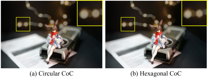
With different lens designs and configurations various CoC styles can be created. Our method can easily simulate this phenomenon by changing the shape of blur kernel. For example, we use a deformable polygonal kernel to create various DoF effects in Fig. 9.

Figure 9. Visualization of adjustable CoC shape rendering, such as (a) circular and (b) hexagonal.

Rendering various views.

5.6. Parameter Analysis

Figure 10. Visualization of inferred aperture and focus parameters. The orange lines represent the initialized values, and we scale the aperture parameters by $10$. Some parameters remain unchanged because the corresponding views are held out for testing and not optimized during training.

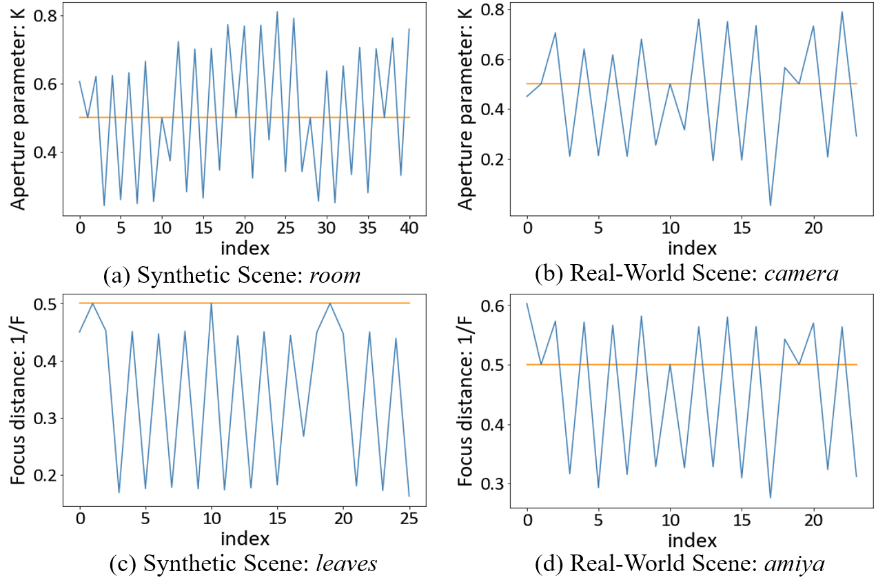
In this section, we construct image sets with mixing patterns to verify the validity of the estimated aperture parameters and focus distances, because accurate apertures and focus distances cannot be obtained in both the real-world dataset and synthetic dataset. Specifically, when validating the focus distance, we use foreground-focused images as even-indexed views, and background-focused images as odd-indexed views. When validating the aperture parameter, on odd-indexed views we use all-in-focus images, which can be seen as images taken using small aperture; on even-indexed views we use shallow DoF images, which can be seen as images taken using wide aperture. We visualize the value of apertures and focus distances of every image before and after optimization in Fig. 10. The results show that the prediction of both aperture parameters and focus distances are optimized to the similar mixing pattern of the training set, which demonstrates that the estimated aperture parameters and focus distances are reasonable and valid.

Table 5. Ablation studies of components of our model. “Aperture” and “Focus” denote learnable aperture parameters and focus distances respectively.

Scene	Model	Aperture	Focus	PSNR$(\uparrow)$	SSIM$(\uparrow)$	LPIPS$(\downarrow)$
camera	NeRF	–	–	25.742	0.8723	0.1657
	ours	$\checkmark$	$\times$	26.639	0.8989	0.1338
	ours	$\times$	$\checkmark$	25.855	0.8786	0.1532
	ours	$\checkmark$	$\checkmark$	26.962	0.9045	0.1280

To validate the design choice of our approach, we also conduct an ablation study on the scene camera. From the results of different combinations in Table 5, one can observe that, i) explicit modeling of the aperture parameters and the focus distance benefits novel view synthesis, and ii) the aperture parameter and the focus distance can promote each other when they are jointly optimized.

6. Conclusion

In this work, we present DoF-NeRF, a novel framework for recovering sharp 3D scenes from sparse shallow DoF images. To achieve this, we model the CoC to simulate the radiance scattered between rays and introduce learnable parameters to enable direct manipulation of the DoF effect. Comprehensive experiments are conducted on both synthetic and real-world datasets, where DoF-NeRF not only performs comparably with NeRF in the all-in-focus setting, but also can synthesize all-in-focus novel views conditioned on shallow DoF inputs. Moreover, by changing the aperture parameter or the focus distance, DoF-NeRF can achieve controllable DoF rendering from novel viewpoints.

Appendix A Appendix Summary

The appendix involves the following contents:

• Table of notations (Table 6).

• Physical model of DoF.

• Algorithm details of the concentrate-and-scatter method.

• Implementation details.

• Datasets details.

• Full experimental reports and more qualitative results.

• More synthesis of DoF effect.

Table 6. Table of notations

Notation	Description
$N$	Number of the images in the training set
$N_{s}$	Number of the sample points on a single ray
$N_{patch}$	Size of the ray patches
$N_{anchor}$	Distance between adjacent anchors
$N_{iters}$	Number of iterations for joint optimization
$N_{pretrain}$	Number of iterations for the first-stage optimization
$\bm{x}$	Spatial location
$\bm{d}$	Viewing direction
$\bm{o}$	Camera origin
$\bm{p}$	Pixel on the imaging plane
$\bm{r}_{\bm{p}}$	Ray specific to pixel $\bm{p}$
$\bm{c}$	Radiance predicted by MLP
$\alpha$	Transparency predicted by MLP
$f$	Focal length
$D$	Aperture diameter
$K$	Aperture parameter
$F$	Focus distance
$h$	Depth of a spatial point along a ray
$\Delta$	Distance between adjacent sample points
$h_{c}$	Concentrated depth
$\delta$	Diameter of CoC
$\delta_{c}$	Diameter of CoC at the concentrated depth
$\mathcal{I}$	Set of input images
$\mathcal{P}$	Set of pixels
$\mathcal{K}$	Set of aperture parameters
$\mathcal{F}$	Set of focus distances
$G_{\Theta},\Theta$	MLP network of NeRF and its parameters
$\mathcal{L}$	Loss
$I$	Input image
$T$	Accumulated transmittance
$\hat{I}(\bm{p})$	Predicted color of a pixel $\bm{p}$
$\hat{I}_{ray}(\bm{p})$	Diffused radiance of a pixel $\bm{p}$
$\hat{I}_{scatter}(\bm{p})$	Scattering radiance from other rays
$\hat{C}$	Scattering radiance of a spatial point
$\hat{C}_{s}(\bm{p})$	Diffused radiance of a pixel $\bm{p}$
$K_{volume}$	Volume rendering coefficient

Appendix B optics principle of DoF

Figure 11. Principle of CoC and DoF.

Visualization of real-world dataset.

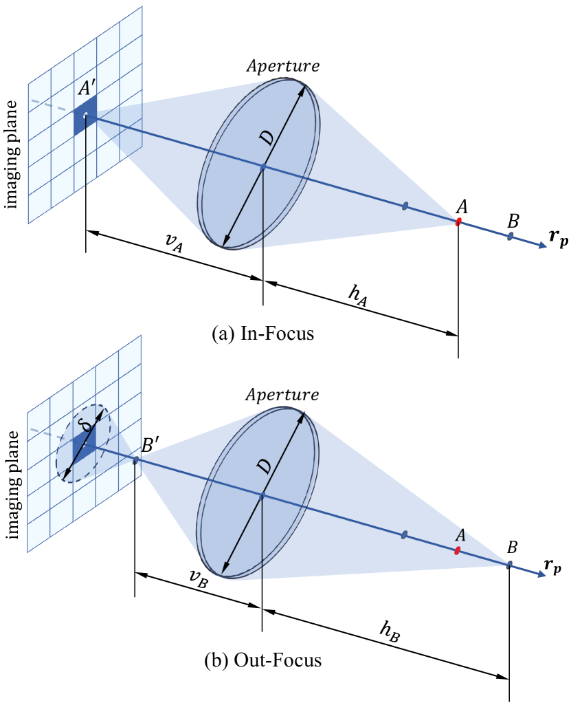
In this section, we provide a detailed derivation of CoC diameters. Given an ideal optical lens system with focal length $f$ and aperture diameter $D$, lights emitted from spatial points $A$ and $B$ on the ray $\bm{r}_{\bm{p}}$ with object distance $h_{A}$ and $h_{B}$ converge on points $A^{\prime}$ and $B^{\prime}$ with imaging distance $v_{A}$ and $v_{B}$, respectively (Fig. 11). The relation between $h_{A}$ and $v_{A}$ (similarly, $h_{B}$ and $v_{B}$) follows the Gaussian formula

(15) $$\vspace{-5pt}\frac{1}{h_{A}}+\frac{1}{v_{A}}=\frac{1}{f}\,,$$

(16) $$\frac{1}{h_{B}}+\frac{1}{v_{B}}=\frac{1}{f}\,.$$

As shown in Fig 11, point $A$ is imaged to the converging point $A^{\prime}$ on the imaging plane. In contrast, point $B$ is projected to a CoC with diameter $\delta_{B}$ on the imaging plane. According to the properties of similar triangles, $\delta_{B}$ can be computed by

(17) $$\frac{\delta_{B}}{D}=\frac{v_{A}-v_{B}}{v_{B}}\,.$$

Substituting Eq.(15) and Eq.(16) into Eq.(17) takes the form

(18) $$\delta_{B}=fD\times\frac{h_{B}-h_{A}}{h_{B}(h_{A}-f)}\,.$$

As the lens system focuses on point $A$, we can replace $h_{A}$ with focus distance $F$:

(19) $$\delta_{B}=fD\times\frac{h_{B}-F}{h_{B}(F-f)}\,.$$

For an out-focus point $C$ with object distance $h_{C}$ smaller than focus distance $F$, the diameter of CoC $\delta_{C}$ is formed as

(20) $$\delta_{C}=fD\times\frac{F-h_{C}}{h_{C}(F-f)}\,.$$

Thus the diameter of CoC can be formulated by

(21) $$\delta=fD\times\frac{\left|F-h_{t}\right|}{h_{t}(F-f)}\,,$$

where $h_{t}$ denotes the object distance of a spacial point. Since the focus distance $F$ and object distance $h_{t}$ are often much larger than the focal length $f$, we can modify Eq. (21) such that

(22) $$\delta(h_{t})=fD\times\frac{\left|h_{t}-F\right|}{Fh_{t}}=fD\times\left|\frac{1}{F}-\frac{1}{h_{t}}\right|\,.$$

Appendix C Algorithm Details

Here we present the implementation details of the Concentrate-and-Scatter algorithm.

As mentioned in the main paper, the concentration of the radiance follows the original volume rendering. We implement the radiance scattering method by a pixel-wise rendering algorithm (see Algorithm 2). Assuming that the aperture shape is circular, we first compute the signed defocus map $S$ with concentrated depth $H_{c}$, aperture parameter $K$ and focus distance $F$. We apply a gamma transformation to transform radiance $C$ to linear space. Two accumulation buffers $W$ and $I$ are initialized with zero. Function TraversePatch() is adopted to traverse all pixels of $C$. The scattering radius $r_{i}$ can be calculated by the absolute value of $S_{i}$. We then traverse the neighboring pixels of $p_{i}$ by the function TraverseNeighbor(). We calculate the weight $w_{i}$ from $p_{i}$ to its neighboring pixel $p_{j}$. For pixel $p_{i}$, its radiance can only scatter to $p_{j}$ if scattering radius $r_{i}$ is larger than the distance $l_{ij}$ between $p_{i}$ and $p_{j}$.

To produce smooth and natural DoF effect, a soft CoC kernel in the calculation of weight $w_{ij}$ is adopted. We additionally divide $w_{ij}$ by the square of $r_{i}$ due to the uniform distribution of radiance. The calculated $w_{ij}$ and radiance $C_{i}$ weighted by $w_{ij}$ are then accumulated in $W_{j}$ and $I_{j}$, respectively. After traversing all pixels, the rendering result $B_{cr}$ can be obtained by the element-wise division of $I$ and $W$. A inverse gamma transformation is applied subsequently.

To create polygonal CoC, we can modify row 8 by multiplying a factor $k_{ij}$ to $r_{i}$. The factor $k_{ij}$ is defined by

(23) $$k_{ij}=\frac{sin\left(\frac{\pi}{2}-\frac{\pi}{n}\right)}{sin\left(\frac{\pi}{2}-\frac{\pi}{n}+mod\left(\left|arctan\left(\frac{l_{ij}^{y}}{l_{ij}^{x}}\right)+\phi\right|,\frac{2\pi}{n}\right)\right)}\,,$$

where $n$ denotes the number of aperture blades and $\phi$ represents the rotation angle of polygonal CoC. $l_{ij}^{x}$ and $l_{ij}^{y}$ denote the horizontal and vertical component of distance $l_{ij}$.

1

Input: Concentrated radiance $C$, concentrated depth $H_{c}$, aperture parameter $K$, focus distance $F$, gamma value $\gamma$

Output: Scattering result $B_{cr}$

2 $S\leftarrow K\cdot(\frac{1}{H_{c}}-\frac{1}{F})$ ;

3 $C\leftarrow(C)^{\gamma}$ ;

4 $W\leftarrow[0]$ ;

5 $I\leftarrow[0]$ ;

6 for $p_{i}\leftarrow$ TraversePatch ($C$) do

7       $r_{i}\leftarrow\lvert S_{i}\rvert$ ;

8       for $p_{j}\leftarrow$ TraverseNeighbor ($p_{i},r_{i}$) do

9             $w_{ij}\leftarrow\frac{0.5+0.5\tanh{(4(r_{i}-l_{ij}))}}{{r_{i}}^{2}+0.2}$ ;

10             $W_{j}\leftarrow W_{j}+w_{ij}$ ;

11             $I_{j}\leftarrow I_{j}+w_{ij}\cdot C_{i}$ ;

12            

13       end for

14      

15 end for

16$B_{cr}\leftarrow\dfrac{I}{W}$ ;

17 $B_{cr}\leftarrow(B_{cr})^{\frac{1}{\gamma}}$ ;

Algorithm 2 Pixel-wise scattering method

Appendix D Implementation Details

We use a batch size of 1024 rays for NeRF and DS-NeRF. The learning rate of NeRF and DS-NeRF is set to $0.0005$ and decays exponentially to one-tenth for every $250000$ steps. For NeRF and DS-NeRF, we use 64 samples for the coarse network and 64 samples for the fine network. As explained in the main paper, we adopt a two-stage optimization: each stage takes $200k$ iterations, where $N_{pretrained}$ and $N_{iters}$ are set to $200k$ and $400k$, respectively. For all-in-focus inputs, we change $N_{pretrained}$ and $N_{iters}$ to $400k$ and $800k$, respectively. At the second optimization stage, we set $N_{patch}$ to 48 and $N_{anchor}$ to 16. The aperture and focus parameters are both initialized with 0.5 for DoF-NeRF. For ablation study, the aperture and focus parameters are set to 0.5 for initialization and fixed according to the experiment settings.

Appendix E Dataset Details

E.1. Real-World Dataset

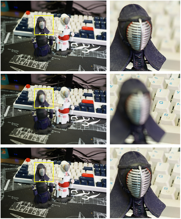
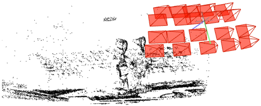
The real-world dataset consists of 7 scenes: amiya, camera, plant, kendo, desk, shelf, and turtle. Each scene contains $20\sim 30$ image triplets. Each triplet includes a wide DoF image taken with small aperture and two images taken with large aperture focusing on the foreground and background respectively (Fig. 12).

Figure 12. Visualization of the scene kendo in the real-world dataset. Each row respectively represents the foreground-focusing shallow DoF image, background-focusing shallow DoF image, and wide DoF image. We zoom in the yellow boxes in the images and present them on the right.

Visualization of real-world dataset.

Figure 13. Visualization of the predicted camera poses and reconstructed sparse point cloud by COLMAP (Schonberger and Frahm, 2016).

Visualization of colmap camera poses.

Figure 14. Visualization of the scene leaves in the synthetic dataset. The first row shows the original image from the Real Forward-Facing dataset (Mildenhall et al., 2020) and the predicted disparity map from DPT (Ranftl et al., 2021). The second and third rows are the shallow DoF images rendered by BokehMe (Peng et al., 2022). We zoom in the yellow boxes in the images and present them on the right.

Visualization of synthetic dataset.

All images are taken by a Sony ILCE-7RM2 camera with an FE 35mm f/1.8 lens. We secure the camera to a tripod and use remote control when taking images, in order to preserve identical camera parameters. Instead of using the maximum aperture to create shallow DoF, we use the aperture of $f/4$ to avoid distinct lens distortion and vignette. The camera parameters are generated by COLMAP (Schonberger and Frahm, 2016). As an example, we visualize the predicted camera poses and sparse point cloud of the scene kendo in Fig. 13. The original resolution of the images in the real-world dataset is $3976\times 2652$. We set the resolution to $497\times 331$ for training and evaluation.

E.2. Synthetic Dataset

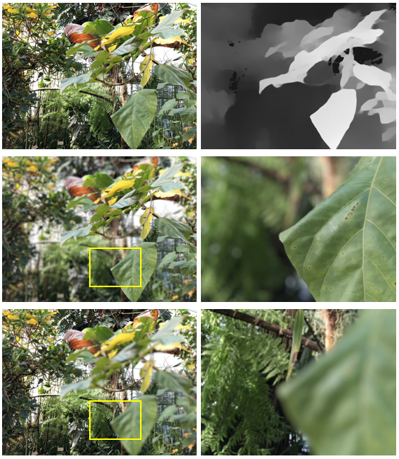
The synthetic dataset is generated from the Real Forward-Facing dataset (Mildenhall et al., 2020) which consists of 8 scenes: fern, flower, fortress, horns, leaves, orchids, room, and trex. Since the images are captured with a handheld cellphone, the original images from the Real Forward-Facing dataset are used as wide DoF images in the triplets. The shallow DoF images are generated based on depth estimation and a recent single-image bokeh rendering framework. For each wide DoF image, we use DPT (Ranftl et al., 2021) to generate the disparity map and BokehMe (Peng et al., 2022) to synthesize the shallow DoF images. The blur parameter of BokehMe is set to 20 and the focus distances are set to 0.1 and 0.9 to simulate background focused and foreground focused shallow DoF images (Fig. 14). The original resolution of the images in the synthetic dataset is $4032\times 3024$. We set the resolution to $504\times 378$ for training and evaluation.

Appendix F Experimental Results

In this section, we present full reports of experiments conducted in main paper and more qualitative comparisons.

Table 7. Comparison of NeRF (Mildenhall et al., 2020) and our framework in the real-world dataset.

Scene	Model	PSNR$(\uparrow)$	SSIM$(\uparrow)$	LPIPS$(\downarrow)$
amiya	NeRF	26.924	0.9092	0.1633
	ours	28.311	0.9289	0.1370
camera	NeRF	25.593	0.8862	0.1574
	ours	27.714	0.9134	0.1259
plant	NeRF	28.272	0.8961	0.1581
	ours	30.317	0.9290	0.1178
turtle	NeRF	33.531	0.9566	0.0939
	ours	34.965	0.9647	0.0823
kendo	NeRF	18.457	0.6643	0.2906
	ours	19.311	0.6970	0.2773
desk	NeRF	29.618	0.9374	0.1099
	ours	30.548	0.9426	0.1047
shelf	NeRF	31.552	0.9515	0.0811
	ours	32.002	0.9565	0.0723

We extend Table 2 and Table 1 in the main paper by conducting experiments in other scenes of the synthetic dataset and real-world dataset. Table 7 and Table 8 report the rendering quality of vanilla NeRF and our model in the real-world dataset and synthetic dataset, respectively. Fig. 17 and Fig. 18 respectively show additional qualitative results using the real-world and synthetic shallow DoF inputs. Given shallow DoF inputs, our method demonstrates better perceptual qualities than vanilla NeRF when rendering all-in-focus novel views on both the real-world dataset and synthetic dataset.

Table 8. Comparison of NeRF (Mildenhall et al., 2020) and our framework in the synthetic dataset.

Scene	Model	PSNR $(\uparrow)$	SSIM$(\uparrow)$	LPIPS$(\downarrow)$
fortress	NeRF	28.142	0.7826	0.2011
	ours	29.168	0.8099	0.1830
leaves	NeRF	19.450	0.6541	0.3190
	ours	20.025	0.7000	0.2766
room	NeRF	26.668	0.8743	0.1961
	ours	29.443	0.9135	0.1502
trex	NeRF	24.433	0.8379	0.1723
	ours	25.726	0.8744	0.1564
fern	NeRF	23.202	0.7232	0.3125
	ours	23.407	0.7311	0.3055
flower	NeRF	26.339	0.8209	0.1999
	ours	27.075	0.8474	0.1678
horns	NeRF	24.260	0.7554	0.2983
	ours	24.829	0.7766	0.2759
orchids	NeRF	19.755	0.6401	0.2932
	ours	20.048	0.6678	0.2718

Table 9. Comparison of DSNeRF (Deng et al., 2022) and our framework in the synthetic dataset.

Scene	Model	PSNR$(\uparrow)$	SSIM$(\uparrow)$	LPIPS$(\downarrow)$
fortress	DSNeRF	28.493	0.7609	0.2373
	ours	29.704	0.8112	0.1970
leaves	DSNeRF	17.872	0.5096	0.4358
	ours	18.312	0.5689	0.3840
room	DSNeRF	26.8301	0.8641	0.2287
	ours	29.550	0.9045	0.1817
trex	DSNeRF	22.334	0.7063	0.3438
	ours	23.600	0.7764	0.2773
fern	NeRF	23.100	0.7050	0.3355
	ours	23.640	0.7307	0.3116
flower	NeRF	25.388	0.7683	0.2517
	ours	26.392	0.8131	0.2024
horns	NeRF	21.562	0.5938	0.4625
	ours	22.487	0.6491	0.4111
orchids	NeRF	19.435	0.6017	0.3247
	ours	19.872	0.6500	0.2876

Table 9 shows the rendering quality of our method using DS-NeRF as baseline on all scenes from the synthetic dataset. Our method can work as a plug-and-play module to improve the performance of NeRF-based method with shallow DoF inputs. Qualitative results are visualized in Fig. 16.

Although our framework is originally designed for shallow DoF inputs, Table 10 indicates that it shows comparable performance against vanilla NeRF using all-in-focus images as inputs.

Table 10. Comparison of NeRF (Mildenhall et al., 2020) and our framework in the all-in-focus dataset.

Scene	Model	PSNR$(\uparrow)$	SSIM$(\uparrow)$	LPIPS$(\downarrow)$
fortress	NeRF	33.973	0.9411	0.0469
	ours	34.007	0.9422	0.0454
leaves	NeRF	21.5860	0.7854	0.1629
	ours	21.4869	0.7861	0.1599
room	NeRF	33.852	0.9593	0.0721
	ours	33.760	0.9584	0.0735
trex	NeRF	30.287	0.9501	0.0601
	ours	30.222	0.9499	0.0605
fern	NeRF	26.582	0.8490	0.1480
	ours	26.565	0.8497	0.1470
flower	NeRF	30.135	0.9221	0.0643
	ours	30.093	0.9224	0.0626
horns	NeRF	28.205	0.8879	0.1332
	ours	28.165	0.8888	0.1313
orchids	NeRF	20.831	0.7362	0.1896
	ours	20.795	0.7374	0.1876

Table 11 shows the results of the ablation study conducted on scene room from the synthetic dataset and on the scene camera from the real-world dataset.

Table 11. Ablation studies of components of our model. “Aperture” and “Focus” denote learnable aperture parameters and focus distances respectively.

Scene	Model	Aperture	Focus	PSNR$(\uparrow)$	SSIM$(\uparrow)$	LPIPS$(\downarrow)$
room	NeRF	–	–	27.279	0.8863	0.1803
	ours	$\checkmark$	$\times$	27.799	0.8992	0.1640
	ours	$\times$	$\checkmark$	28.070	0.9032	0.1671
	ours	$\checkmark$	$\checkmark$	28.361	0.9076	0.1556
camera	NeRF	–	–	25.742	0.8723	0.1657
	ours	$\checkmark$	$\times$	26.639	0.8989	0.1338
	ours	$\times$	$\checkmark$	25.855	0.8786	0.1532
	ours	$\checkmark$	$\checkmark$	26.962	0.9045	0.1280

Appendix G DoF Rendering

Figure 15. More synthesis of controllable DoF effect. DoF-NeRF can manipulate the DoF rendering by changing (a) aperture size and focus distance, (b) camera poses, (c) perspective, and (d) aperture shape.

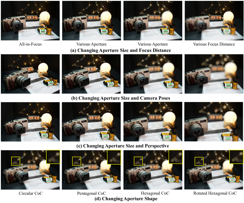
In this section, we present more synthesis of controllable DoF rendering (Fig. 15). Benefiting from the explicit modeling of DoF effect, DoF-NeRF enables direct manipulation of DoF effect by adjusting virtual aperture size and focus distance. Compared with single-image DoF rendering method, DoF-NeRF is capable of rendering DoF effect from novel viewpoints by adjusting the corresponding camera parameters. With different lens designs and configurations such as the shape of aperture, various CoC styles can be created. Our concentrate-and-scatter method can easily simulate this phenomenon by changing the shape of blur kernel. For example, we use a deformable polygonal kernel to create various DoF effects.

Appendix H Cost of Training and Testing

We compare the training and testing time of DoF-NeRF and vanilla NeRF on the same machine using a single NVIDIA RTX 3090 GPU. The following report are measured on the Scene Camera from the real-world dataset.

H.1. Training

We train each model for a total of $400k$ iterations, i.e., $400k$ iterations for vanilla NeRF, $200k$ iterations each for the first and second stage of DoF-NeRF. The batch size is set to $1024$ rays for NeRF and the first stage of DoF-NeRF. We set $N_{patch}$ to $32$ in order to calculate the same amount of rays in every iteration.

• Vanilla NeRF takes $6h26min$.

• DoF-NeRF takes $6h41min$, $3.8\%$ longer than vanilla NeRF.

Both models take about 6GB GPU memory during training.

H.2. Testing

We render 120 images from different viewpoints using NeRF and DoF-NeRF model. All the synthesized images are of $497\times 331$ resolution.

• Vanilla NeRF takes $403s$, i.e., $3.36s$ per image.

• DoF-NeRF takes $405s$, i.e., $3.38s$ per image, $0.60\%$ longer than vanilla NeRF.

Figure 16. Additional comparison of DS-NeRF (Deng et al., 2022) and our approach in the synthetic dataset. For each scene, the zoom-in of rendered images and error maps ($0$ to $0.2$ pixel intensity range) are presented. They are respectively obtained from DS-NeRF (first row) and our model (second row). For each subfigure, PSNR is shown on the lower left.

Figure 17. Additional comparison of NeRF (Mildenhall et al., 2020) and our approach with shallow DoF inputs on the real-world dataset. The first and third column show the images rendered by NeRF and our approach, respectively. PSNR is shown at the upper left corner. We zoom in all the yellow boxes and present them in the second and fourth column with error maps ($0$ to $0.1$ pixel intensity range) shown at the lower right corner.

Figure 18. Additional comparison of NeRF (Mildenhall et al., 2020) and our approach with shallow DoF inputs on the synthetic dataset. The first and third column show the images rendered by NeRF and our approach, respectively. PSNR is shown at the upper left corner. We zoom in all the yellow boxes and present them in the second and fourth column with error maps ($0$ to $0.1$ pixel intensity range) shown at the lower right corner.