Possible zero sound in layered perovskites with ferromagnetic s-d exchange interaction

Abstract

We analyze the conditions for observation of zero sound in layered perovskites with transition metal ion on chalcogenide oxidizer. We conclude that propagation of zero sound is possible only for a ferromagnetic sign of the s-d interaction. If the s-d exchange integral J$\!{}_{sd}$ has antiferromagnetic sign, as it is perhaps in the case for layered cuprates, zero sound is a thermally activated dissipation mode, which generates only “hot spots” in the Angle Resolved Photoemission Spectroscopy (ARPES) data along the Fermi contour. We predict that zero sound will be observable for transition metal perovskites with 4s and 3d levels close to the p-level of the chalcogenide. The simultaneous lack of superconductivity, the appearance of hot spots in ARPES data, and the proximity of the three named levels, represents the significant hint for the choice of material to be investigated.

I Introduction

The theoretical prediction of zero sound by Landau [1, 2] and subsequent experimental observations [3, 4] in ³He was a powerful evidence of the applicability of Landau picture of Fermi quasi-particles excitations and their self-consistent motion to (strongly correlated) Fermi liquids. The zero Fermi sound in metals, more precisely zero spin sound, was observed in Cr metal [6, 7]. These experiments stimulated studies in the framework of the Hubbard model. Fuseya et al. [8] reached the important, to our further analysis, conclusion that Landau parameter, i.e. the averaged on the Fermi surface Fermi liquid interaction kernel $f(\mathbf{p},\mathbf{q})$, can change its sign close to half filling of the conduction band. Later on Tsuruta [9] used two dimensional $t$-$t^{\prime}$ Hubbard model to study zero spin sound in antiferromagnetic metals. Here, we consider that this approach can be useful to study zero sound propagation and its importance from a materials science perspective. The purpose of the present paper is to explore the possibility of zero sound propagation in a layered perovskite with the structure of high-$T_{c}$ having a CuO₂ conduction plane.

Postulating the interaction kernel $f(\mathbf{p},\mathbf{q})$ [10, Eq. (2.1)] between electrons with different momenta $\mathbf{p}$ and $\mathbf{q}$, we can explain different electronic phenomena in superconductivity and magnetism. The Fermi liquid approach provides results for the magnetic susceptibility, heat capacity, and effective masses. For illustration, in many cases the interaction is modeled by a separable kernel $f(\mathbf{p},\mathbf{q})\propto\chi(\mathbf{p})\chi(\mathbf{q})$ and for our Hamiltonian separability holds.

The $s$-$d$ exchange lies in the origin of the magnetic properties of transition metal compounds. Its most usual version was proposed by Schubin and Wonsovsky [11], Zener [12, 13, 14] and Kondo [15]. The purpose of the present study is to analyze whether the $s$-$d$ exchange can lead to propagation of zero sound in transition metal compounds.

We anticipate here, that an anti-ferromagnetic sign of the $s$-$d$ coupling $J_{sd}$ leads to a singlet superconductivity while a ferromagnetic sign of $J_{sd}$ is able to explain the repulsion necessary for the propagation of zero sound. We wish to emphasize that zero sound has not yet been observed in normal metals [16]. This may be traced back to the fact that the $s$-$d$ exchange interaction was not used as a guide for the choice of appropriate materials.

In the next section we introduce the notions and notations developed to explain the electronic properties of the CuO₂ plane and its superconductivity, and analyze how a similar Hamiltonian would be used to predict zero sound in layered cuprates. Finally, we conclude that layered transition metal compounds may serve as the best candidates to search for zero sound in normal metals.

II The s-d LCAO Hamiltonian for the CuO₂ plane in momentum $\mathbf{p}$-representation

The Hamiltonian in the $\mathbf{r}$-representation is given in Ref. [17, Eq. (1.2)], here we start with the Hamiltonian in the $\mathbf{p}$-representation

$$\hat{H}^{\prime}= \sum_{\mathbf{p},\,\alpha}\hat{\Psi}_{\mathbf{p}}^{\dagger}\left(H_{\mathrm{LCAO}}-\mu\mathbb{1}\right)\hat{\Psi}_{\mathbf{p}}$$

$$-\frac{J_{sd}}{\mathcal{N}}\sum_{\begin{subarray}{c}\mathbf{p}^{\prime}+\mathbf{q}^{\prime}=\mathbf{p}+\mathbf{q}\\ \alpha,\,\beta\end{subarray}}\hat{S}_{\mathbf{q}^{\prime},\beta}^{\dagger}\hat{D}_{\mathbf{p}^{\prime},\alpha}^{\dagger}\hat{S}_{\mathbf{p},\alpha}\hat{D}_{\mathbf{q},\beta},$$ (1)

where

$$H_{\mathrm{LCAO}}\equiv\begin{pmatrix}\epsilon_{d}&0&t_{pd}s_{x}&-t_{pd}s_{y}\\ 0&\epsilon_{s}&t_{sp}s_{x}&t_{sp}s_{y}\\ t_{pd}s_{x}&t_{sp}s_{x}&\epsilon_{\mathrm{p}}&-t_{pp}s_{x}s_{y}\\ -t_{pd}s_{y}&t_{sp}s_{y}&-t_{pp}s_{x}s_{y}&\epsilon_{\mathrm{p}}&\end{pmatrix},$$

$$s_{x}\equiv 2\sin(p_{x}/2),\qquad s_{y}\equiv 2\sin(p_{y}/2),\\$$

$$\hat{\Psi}_{\mathbf{p}}^{\dagger}\equiv\begin{pmatrix}\hat{D}^{\dagger}_{\mathbf{p},\alpha}&\hat{S}^{\dagger}_{\mathbf{p},\alpha}&\hat{X}^{\dagger}_{\mathbf{p},\alpha}&\hat{Y}^{\dagger}_{\mathbf{p},\alpha}\end{pmatrix},$$

and the summation is actually an integration in the momentum space and $\mathcal{N}\gg 1$ is the total number of elementary cells for which we assume periodic boundary conditions

$$\frac{1}{\mathcal{N}}\sum_{\mathbf{p}}\dots\;\;\equiv\iint\limits_{\{p_{x},p_{y}\}\in(0,2\pi)}\frac{\mathrm{d}p_{x}\mathrm{d}p_{y}}{(2\pi)^{2}}\dots$$

where the momentum variables are dimensionless phases $p_{x},p_{y},q_{x},q_{y}\in(0,2\pi)$; the dimensional momentum is $\mathbf{P}=(\hbar/a_{0})\,\mathbf{p}.$ In this LCAO Hamiltonian $\epsilon_{s}$, $\epsilon_{d}$ and $\epsilon_{p}$ are the single site energies of an electron in Cu4$s$, Cu3$d_{x^{2}-y^{2}}$ and O2$\mathrm{p}$ states, $t_{sp}$, $t_{pd}$ and $t_{pd}$ are hopping amplitudes between neighboring orbitals. The $s$-$d$ interaction is parameterized by the exchange integral $J_{sd}$ which we consider as a perturbation. Schematically, the atomic wave functions are depicted in Fig. 1. The chemical potential is denoted by $\mu$ and for the operator of the number of electrons we have the standard expression

$$\hat{N} =-\partial_{\mu}\hat{H}^{\prime}$$

$$=\sum_{\mathbf{p},\,\alpha}(\hat{D}_{\mathbf{p},\alpha}^{\dagger}\hat{D}_{\mathbf{p},\alpha}+\hat{S}_{\mathbf{p},\alpha}^{\dagger}\hat{S}_{\mathbf{p},\alpha}+\hat{X}_{\mathbf{p},\alpha}^{\dagger}\hat{X}_{\mathbf{p},\alpha}+\hat{Y}_{\mathbf{p},\alpha}^{\dagger}\hat{Y}_{\mathbf{p},\alpha}),$$

which we treat self-consistently.

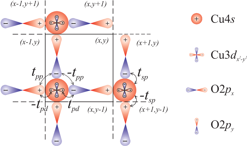
Figure 1: Single electron processes in the conducting CuO₂ plane of layered cuprates after Ref. [17, Fig. 1.1]. LCAO is the basis of the chemical intuition. We have Hilbert space spanned over Cu$4s$, Cu$3d_{x^{2}-y^{2}}$, O$2p_{x}$, and O$2p_{y}$ states. The LCAO Hamiltonian is parameterized by transfer integrals $t_{pd}$, $t_{sp}$, and $t_{pp}$ and single site energies $\epsilon_{d}$, $\epsilon_{s}$, $\epsilon_{p}$.

II.1 Conduction band reduction

In order to derive the effective Hamiltonian describing the zero sound, we perform successive conduction band reductions. The first one is the number of particles. For notions and notations we follow the description of the electronic properties of the CuO₂ plane. In the hole doped phase of the CuO₂ plane we have 2 completely filled oxygen bands O$2p$ and one partially filled Cu3$d_{x^{2}-y^{2}}$band, $f$ is the relative number of holes in the Brillouin zone, i.e. the hole filling factor defined as the ratio of the area of the hole pocket around the $(\pi,\,\pi)$ point and the area of the Brillouin zone is $(2\pi)^{2}$. For the averaged number of electrons we have

$$\langle\hat{N}\rangle/{\mathcal{N}}=2\times 2+2(1-f).$$ (2)

For $f=\frac{1}{2}$ we have a pattern insulator, while for optimal doping we have

$$f_{\mathrm{opt}}=\frac{1}{2}+0.08.$$ (3)

The single electron component of the Hamiltonian is diagonalized in the $\mathbf{p}$-representation and we have to perform the summation over all four bands $b=1,2,3,4$

$$\hat{H}^{\prime(0)} =\sum_{\mathrm{b},\mathbf{p},\alpha}(\epsilon_{\mathrm{b},\mathbf{p}}-\mu)\hat{c}_{\mathrm{b},\mathbf{p},\alpha}^{\dagger}\hat{c}_{\mathrm{b},\mathbf{p},\alpha}$$

$$\rightarrow\sum_{\mathbf{p},\alpha}(\epsilon_{\mathbf{p}}-\mu)\,\hat{c}_{\mathbf{p},\alpha}^{\dagger}\hat{c}_{\mathbf{p},\alpha}.$$ (4)

The spectrum $\mathbf{p}$ in the LCAO approximation is determined by the secular equation

$$\mathrm{det}[H_{\mathrm{LCAO}}-\epsilon_{\mathbf{p}}\openone]=\mathcal{A}xy+\mathcal{B}(x+y)+\mathcal{C}=0,$$

where the variables

$$x=\sin^{2}\left(\frac{p_{x}}{2}\right),\qquad y=\sin^{2}\left(\frac{p_{y}}{2}\right),$$

are functions only of the momentum $\mathbf{p}$, and

$$\mathcal{A} =32\left(t_{sp}^{2}-\frac{1}{2}\varepsilon_{s}t_{pp}\right)^{2}(2t_{pd}^{2}+t_{pp}\varepsilon_{d}),$$

$$\mathcal{B} =-4\varepsilon_{\mathrm{p}}(t_{sp}^{2}\varepsilon_{d}+t_{pd}^{2}\varepsilon_{s}),$$

$$\mathcal{C} =\varepsilon_{d}\varepsilon_{s}\varepsilon_{\mathrm{p}}^{2},$$

are polynomials of the energy $\epsilon$. This analytical representation of the energy dispersion $\epsilon_{\mathbf{p}}$ allows to express explicitly its derivatives

$$\mathbf{v}_{\mathbf{p}}=\frac{\partial\epsilon_{\mathbf{p}}}{\partial\mathbf{p}},\quad\mathbf{V}_{\mathbf{p}}=\frac{a_{0}}{\hbar}\mathbf{v}_{\mathbf{p}}=\frac{\mathrm{d}\mathbf{r}}{\mathrm{d}t},\quad\mathbf{P}=\frac{\hbar}{a_{0}}\mathbf{p},$$ (5)

where $\mathbf{P}$ is dimensional momentum and $V_{\mathbf{p}}$ is the velocity in the usual units length per time.

In order to study the low frequency electronic processes, we restrict the Hamiltonian summation only to the conduction band $b=3$ and the index will be dropped; $b=1$ and $b=2$ denote completely filled oxygen bands, while $b=4$ is the index for the completely empty Cu$4s$ band. Performing this first reduction, the interaction $s$-$d$-exchange Hamiltonian reads

$$\hat{H}_{sd}=-\frac{J_{sd}}{\mathcal{N}}\!\!\!\sum_{\begin{subarray}{c}\mathbf{p}^{\prime}+\mathbf{q}^{\prime}=\mathbf{p}+\mathbf{q}\\ \alpha,\,\beta\end{subarray}}\!\!\!S_{\mathbf{q}^{\prime}}D_{\mathbf{p}^{\prime}}{\color[rgb]{0,0,1}\hat{c}^{\dagger}_{\mathbf{q}^{\prime}\beta}\hat{c}^{\dagger}_{\mathbf{p}^{\prime}\alpha}}{\color[rgb]{1,0,0}\hat{c}_{\mathbf{p}\alpha}\hat{c}_{\mathbf{q}\beta}}S_{\mathbf{p}}D_{\mathbf{q}},$$ (6)

where the real amplitudes

$$\begin{pmatrix}\tilde{D}_{\mathbf{p}}\\ \tilde{S}_{\mathbf{p}}\\ \tilde{X}_{\mathbf{p}}\\ \tilde{Y}_{\mathbf{p}}\end{pmatrix}\!\!=\!\!\begin{pmatrix}-\varepsilon_{s}\varepsilon_{\mathrm{p}}^{2}+4\varepsilon_{p}t_{sp}^{2}(x+y)-32t_{pp}\tau_{sp}^{2}xy\\ -4\varepsilon_{\mathrm{p}}t_{sp}t_{pd}(x-y)\\ -(\varepsilon_{s}\varepsilon_{\mathrm{p}}-8\tau_{sp}y)t_{pd}s_{x}\\ (\varepsilon_{s}\varepsilon_{\mathrm{p}}-8\tau_{sp}x)t_{pd}s_{y}\end{pmatrix}$$ (7)

describe the amplitude of a band electron to be projected on Cu4$s$, Cu3$d_{x^{2}-y^{2}}$, O2$p_{x}$ and O2$p_{y}$. For brevity we introduce the notations $\varepsilon_{s}=\epsilon-\epsilon_{s}$, $\varepsilon_{d}=\epsilon-\epsilon_{d}$, $\varepsilon_{\mathrm{p}}=\epsilon-\epsilon_{\mathrm{p}}$. The amplitudes have to be normalized to

$$C_{\Psi}=\frac{1}{\sqrt{D_{\mathbf{p}}^{2}+S_{\mathbf{p}}^{2}+X_{\mathbf{p}}^{2}+Y_{\mathbf{p}}^{2}}},$$

and finally $S_{\mathbf{p}}=C_{\Psi}\tilde{S}_{\mathbf{p}}$, $D_{\mathbf{p}}=C_{\Psi}\tilde{D}_{\mathbf{p}}$. For convenience we introduce the notation describing the $s$-$d$ hybridization amplitude $\chi_{\mathbf{p}}\equiv S_{\mathbf{p}}D_{\mathbf{p}}$ of the band electron. In the next subsection we juxtapose different further reductions of the exchange Hamiltonian treated in a self-consistent way.

II.2 BCS versus Fermi liquid reduction

Our first step is to perform BCS reduction of the exchange Hamiltonian Eq. (6). In the sum we have to take into account only the annihilation and creation operators with opposite momenta and spins

$${\color[rgb]{0,0,1}\mathbf{q}^{\prime}=-\mathbf{p}^{\prime}},\qquad{\color[rgb]{1,0,0}\mathbf{q}=-\mathbf{p}},\qquad\beta=\overline{\alpha}.$$ (8)

In averaging of this BCS reduced Hamiltonian we apply the self-consistent approximation

$$\langle{\color[rgb]{0,0,1}\hat{c}^{\dagger}_{\mathbf{q}^{\prime}\beta}\hat{c}^{\dagger}_{\mathbf{p}^{\prime}\alpha}}{\color[rgb]{1,0,0}\hat{c}_{\mathbf{p}\alpha}\hat{c}_{\mathbf{q}\beta}}\rangle \rightarrow\delta_{\mathbf{q}^{\prime}+\mathbf{p}^{\prime},0}\,\delta_{\mathbf{q}+\mathbf{p},0}\,\langle{\color[rgb]{0,0,1}\hat{c}^{\dagger}_{\mathbf{q}^{\prime}\beta}\hat{c}^{\dagger}_{\mathbf{p}^{\prime}\alpha}}{\color[rgb]{1,0,0}\hat{c}_{\mathbf{p}\alpha}\hat{c}_{\mathbf{q}\beta}}\rangle$$

$$\approx\delta_{\mathbf{q}^{\prime}+\mathbf{p}^{\prime},0}\,\delta_{\mathbf{q}+\mathbf{p},0}\,\langle{\color[rgb]{0,0,1}\hat{c}^{\dagger}_{\mathbf{q}^{\prime}\beta}\hat{c}^{\dagger}_{\mathbf{p}^{\prime}\alpha}}\rangle\langle{\color[rgb]{1,0,0}\hat{c}_{\mathbf{p}\alpha}\hat{c}_{\mathbf{q}\beta}}\rangle$$

$$=\langle{\color[rgb]{0,0,1}\hat{c}^{\dagger}_{-\mathbf{p}^{\prime}\overline{\alpha}}\hat{c}^{\dagger}_{\mathbf{p}^{\prime}\alpha}}\rangle\langle{\color[rgb]{1,0,0}\hat{c}_{\mathbf{p}\alpha}\hat{c}_{-\mathbf{p}\overline{\alpha}}}\rangle=\langle\hat{B}_{\mathbf{p^{\prime}}}\rangle\langle\hat{B}_{\mathbf{p}}\rangle,$$

where

$$\hat{B}_{\mathbf{p}}\equiv\hat{c}_{-\mathbf{p},-}\hat{c}_{\mathbf{p}+}=u_{\mathbf{p}}v_{\mathbf{p}}(1-\hat{b}_{-\mathbf{p},-}^{\dagger}\hat{b}_{-\mathbf{p}-}-\hat{b}_{\mathbf{p},+}^{\dagger}\hat{b}_{\mathbf{p}+})+\dots\;.$$ (9)

Colors (on-line) describe factorization of means in the effective Hamiltonian. The self-consistent approximation is reduced to substitution of averaged product of four operators to the product of averaged two operators. In order to emphasize the basis of the BCS approximation we use different colors. Those colors can be traced back to the conduction band reduced exchange Hamiltonian Eq. (6). We use standard notations for Bogolyubov $u$-$v$ rotation and the new $\hat{B}$ operators with average expressed in terms of new Fermion number operators $\hat{n}_{\mathbf{p},\alpha}=\hat{b}_{\mathbf{p}\alpha}^{\dagger}\hat{b}_{\mathbf{p}\alpha}$. In this way the average exchange Hamiltonian is incorporated in the standard BCS scheme

$$\langle\hat{H}_{sd}^{\mathrm{(BCS)}}\rangle=\frac{1}{\mathcal{N}}\sum_{\mathbf{p}^{\prime},\,\mathbf{p}}\langle\hat{B}_{\mathbf{p^{\prime}}}\rangle f(\mathbf{p}^{\prime},\mathbf{p})\langle\hat{B}_{\mathbf{p}}\rangle,$$ (10)

where the kernel

$$f(\mathbf{p}^{\prime},\mathbf{p})=-2J_{sd}\chi_{\mathbf{p}^{\prime}}\chi_{\mathbf{p}}.$$

is separable due to the fact that the exchange interaction is localized on a single ion in the elementary cell of the crystal.

Now we address the Fermi liquid reduction of the same exchange Hamiltonian Eq. (6) which we rewrite

$$\hat{H}_{sd}=-\frac{J_{sd}}{\mathcal{N}}\!\!\sum_{\begin{subarray}{c}\mathbf{p}^{\prime}+\mathbf{q}^{\prime}=\mathbf{p}+\mathbf{q}\\ \alpha,\,\beta\end{subarray}}\!\!S_{\mathbf{q}^{\prime}}D_{\mathbf{p}^{\prime}}{\color[rgb]{1,0,0}\hat{c}^{\dagger}_{\mathbf{q}^{\prime}\beta}}{\color[rgb]{0,0,1}\hat{c}^{\dagger}_{\mathbf{p}^{\prime}\alpha}\hat{c}_{\mathbf{p}\alpha}}{\color[rgb]{1,0,0}\hat{c}_{\mathbf{q}\beta}}S_{\mathbf{p}}D_{\mathbf{q}}.$$ (11)

In order to point out the difference between BCS and Fermi liquid reduction now the colors mark the operators which will be grouped in the next self-consistent approximation. In the Fermi-liquid (FL) reduced Hamiltonian we have to take into account only the terms with

$${\color[rgb]{0,0,1}\mathbf{p}^{\prime}=\mathbf{p}},\qquad{\color[rgb]{1,0,0}\mathbf{q}^{\prime}=\mathbf{q}}.$$ (12)

In FL reduction we have again to apply the self-consistent approximation for the relevant terms

$$\langle{\color[rgb]{1,0,0}\hat{c}^{\dagger}_{\mathbf{q}^{\prime}\beta}}{\color[rgb]{0,0,1}\hat{c}^{\dagger}_{\mathbf{p}^{\prime}\alpha}\hat{c}_{\mathbf{p}\alpha}}{\color[rgb]{1,0,0}\hat{c}_{\mathbf{q}\beta}}\rangle \rightarrow\delta_{\mathbf{q}^{\prime},\mathbf{q}}\,\delta_{\mathbf{p}^{\prime},\mathbf{p}}\,\langle{\color[rgb]{0,0,1}\hat{c}^{\dagger}_{\mathbf{p}^{\prime}\alpha}\hat{c}_{\mathbf{p}\alpha}}{\color[rgb]{1,0,0}\hat{c}^{\dagger}_{\mathbf{q}^{\prime}\beta}}{\color[rgb]{1,0,0}\hat{c}_{\mathbf{q}\beta}}\rangle$$

$$\approx\delta_{\mathbf{q}^{\prime},\mathbf{q}}\,\delta_{\mathbf{p}^{\prime},\mathbf{p}}\,\langle{\color[rgb]{0,0,1}\hat{c}^{\dagger}_{\mathbf{p}^{\prime}\alpha}\hat{c}_{\mathbf{p}\alpha}}\rangle\langle{\color[rgb]{1,0,0}\hat{c}^{\dagger}_{\mathbf{q}^{\prime}\beta}}{\color[rgb]{1,0,0}\hat{c}_{\mathbf{q}\beta}}\rangle$$

$$=\langle{\color[rgb]{0,0,1}\hat{c}^{\dagger}_{\mathbf{p}\alpha}\hat{c}_{\mathbf{p}\alpha}}\rangle\langle{\color[rgb]{1,0,0}\hat{c}^{\dagger}_{\mathbf{q}\beta}}{\color[rgb]{1,0,0}\hat{c}_{\mathbf{q}\beta}}\rangle=\langle n_{\mathbf{p},\alpha}\rangle\langle n_{\mathbf{q},\beta}\rangle.$$

Analogously to the BCS reduction, now for the FL reduction we obtain the averaged Hamiltonian

$$\langle\hat{H}_{{}_{\mathrm{sd}}}^{\mathrm{(FL)}}\rangle=\frac{1}{\mathcal{N}}\sum_{\mathbf{p},\mathbf{q},\,\alpha,\beta}\langle\hat{n}_{\mathbf{p},\alpha}\rangle f(\mathbf{p},\mathbf{q})\langle\hat{n}_{\mathbf{q},\beta}\rangle,$$ (13)

which is expressed by the same kernel

$$f(\mathbf{p},\mathbf{q})=-2J_{sd}\chi_{\mathbf{p}}\chi_{\mathbf{q}},\\$$

applied between the average numbers of the Fermi particles

$$\hat{n}_{\mathbf{p},\alpha} =\hat{c}^{\dagger}_{\mathbf{p\alpha}}\hat{c}_{\mathbf{p\alpha}},$$

$$\langle\hat{n}_{\mathbf{p},\alpha}\hat{n}_{\mathbf{q},\beta}\rangle \approx\langle\hat{n}_{\mathbf{p},\alpha}\rangle\langle\hat{n}_{\mathbf{q},\beta}\rangle.$$

This coincidence of the kernels of BCS and FL approach is one of the central results of the present study. This coincidence can be explored for application in the study of other layered transition metal perovskites as well.

We wish to emphasize that for the interaction kernel we have analytical results at hand and for the $s$-$d$ hybridization function, we have [17]

$$\chi_{\mathbf{p}}=\ S_{\mathbf{p}}D_{\mathbf{p}}$$

$$=\ 4\varepsilon_{\mathrm{p}}t_{sp}t_{pd}(x-y)$$

$$\times\left[\varepsilon_{s}\varepsilon_{\mathrm{p}}^{2}-4\varepsilon_{\mathrm{p}}t_{sp}^{2}\,(x+y)+32t_{pp}\tau_{sp}^{2}\,xy\right]$$

$$\times\left\{\left[4\varepsilon_{\mathrm{p}}t_{sp}t_{pd}\,(x-y)\right]^{2}\right.$$

$$\qquad+\left[\varepsilon_{s}\varepsilon_{\mathrm{p}}^{2}-4\varepsilon_{\mathrm{p}}t_{sp}^{2}\,(x+y)+32t_{pp}\tau_{sp}^{2}\,xy\right]^{2}$$

$$\qquad+4x\left[(\varepsilon_{s}\varepsilon_{\mathrm{p}}-8\tau_{sp}^{2}y)t_{pd}\right]^{2}$$

$$\qquad\left.+4y\left[(\varepsilon_{s}\varepsilon_{\mathrm{p}}-8\tau_{sp}^{2}x)t_{pd}\right]^{2}\right\}^{-1}.$$ (14)

This hybridization function in the quasi-momentum representation is depicted in Fig. 2.

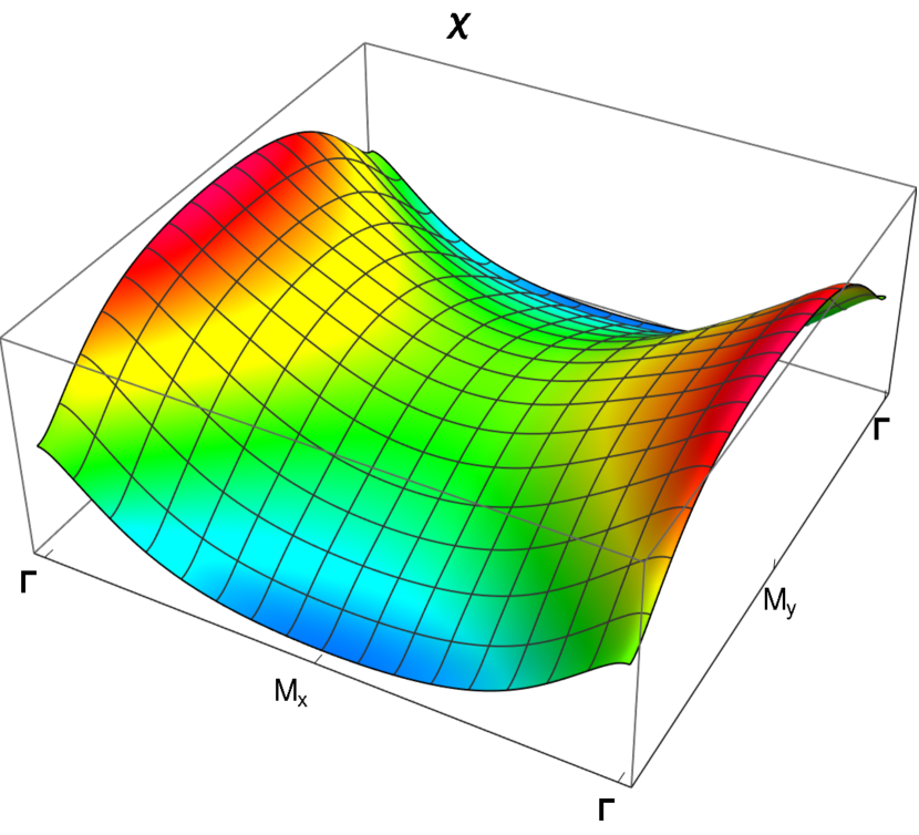
Figure 2: The hybridization function $\chi_{\mathbf{p}}=S_{p}D_{p}$ representing the amplitude electron from conduction Cu3$d_{x^{2}-y^{2}}$ band being simultaneously a Cu$4s$ electron. This is the main ingredient of the matrix elements of the s-d exchange interaction.

One can see that at fixed electron energy this saddle can be approximated by single sinusoidal approximation $\chi\propto\cos(2\theta)$ where $\theta=\arctan(p_{y},p_{x})$. Close to the $(\pi,\,\pi)$-point the single particle spectrum $\epsilon_{\mathbf{p}}$ has a parabolic form $\epsilon_{\mathbf{p}}\approx\epsilon_{\pi,\,\pi}-p^{2}/2\tilde{m}_{\mathrm{eff}}$ and qualitatively this approximation can be extended to the Fermi contour of the optimally doped cuprates.

The band velocity $\mathbf{v}=\partial_{\mathbf{p}}\epsilon_{\mathbf{p}}$ calculated from the real LCAO Hamiltonian is drawn in Fig. 3.

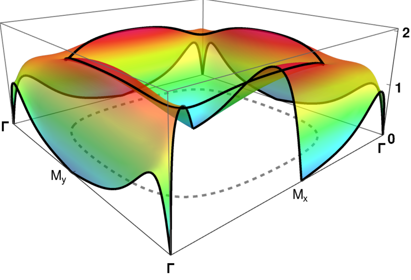
Figure 3: Velocity $v_{\mathbf{p}}$ of the conduction band as a function of quasi-momentum $p_{x},\,p_{y}\in(0,2\pi)$ with dimension energy given in eV. The variable $V=(a_{0}/\hbar)v$ has dimension m/s. In the special points $\Gamma=(0,\,0)$, $\mathrm{M}=(\pi,\,0)$, $\mathrm{X}=(\pi,\,\pi)$ the band velocity $\mathbf{V}=\partial\epsilon_{\mathbf{P}}/\partial\mathbf{P}$ is zero; $\mathbf{P}=(\hbar/a_{0})\mathbf{p}$.

Here we can see that the circular Fermi contour is only a rough initial approximation.

The averaged BCS Hamiltonian has to be minimized with respect to $u_{\mathbf{p}}$ and then the BCS spectrum

$$E_{\mathbf{p}}=\frac{\partial\langle\hat{H}^{\mathrm{(BCS)}}\rangle}{\partial{\langle n_{\mathbf{p},\alpha}\rangle}}=\sqrt{(\epsilon_{\mathbf{p}}-\mu)^{2}+\Delta_{\mathbf{p}}^{2}}.$$ (15)

In the next Section we analyze the possible propagation of zero sound in layered perovskites using the single particle spectrum obtained from the FL reduced Hamiltonian Eq. (13).

III Zero sound dispersion

For a concise introduction to the Fermi liquid approach we recommend the well-known monographs by Nozieres [18], Abrikosov [16], Abrikosov, Gor’kov and Dzyaloshinski [19], Lifshitz and Pitaevskii [10] and [20, Sec. 76].

Introducing for brevity $n_{\mathbf{p},\alpha}\equiv\langle\hat{n}_{\mathbf{p},\alpha}\rangle$, the averaged FL Hamiltonian Eq. (13) reads

$$H_{\mathrm{{}_{FL}}}\equiv\langle\hat{H}^{\mathrm{(FL)}}\rangle=\sum_{\mathbf{p},\,\alpha}\epsilon_{\mathrm{p}}n_{\mathrm{p},\alpha}+\frac{1}{\mathcal{N}}\!\sum_{\mathbf{p},\mathbf{q},\,\alpha,\beta}n_{\mathbf{p},\alpha}f(\mathbf{p},\mathbf{q})n_{\mathbf{q},\beta}.$$ (16)

Notice that the spin indices may be omitted if we consider spin non-polarized phenomena, such that $n_{\mathbf{q},+}=n_{\mathbf{q},-}$. Introducing $n_{\mathbf{q}}\equiv n_{\mathbf{q},+}+n_{\mathbf{q},-}=2n_{\mathbf{q},+}=2n_{\mathbf{q},-}$ for the FL energy spectrum we get

$$\varepsilon(\mathbf{p},\mathbf{r})=\frac{\partial H_{{}_{\mathrm{FL}}}}{\partial\hat{n}_{\mathbf{p}}}=\ \epsilon_{\mathbf{p}}+\frac{1}{\mathcal{N}}\sum_{\mathbf{q}}f(\mathbf{p},\mathbf{q})n_{\mathbf{q}}(\mathbf{r})$$

$$=\ \epsilon_{\mathbf{p}}+\frac{(-2J_{sd})}{\mathcal{N}}\chi_{\mathbf{p}}\sum_{\mathbf{q}}\chi_{\mathbf{q}}n_{\mathbf{q}}(\mathbf{r},t),$$ (17)

where the space variable $\mathbf{r}\equiv a_{0}\mathbf{n}$ can be introduced only in the quasi-classical WKB approximation. The $s$-$d$ hybridization function Eq. (14) determines both the gap anisotropy $\Delta_{\mathbf{p}}(T)=\Xi(T)\chi_{\mathbf{p}}$ and the FL interaction. A detailed analysis of the gap anisotropy and the hot/cold spot anisotropy of ARPES data described by the hybridization function $\chi_{\mathbf{p}}$ in Eq. (14) is presented in Ref. [21]. Now we consider the momentum distribution $n_{\mathbf{p}}(\mathbf{r},t)$ of the charge carriers as dynamic variables. Assuming a local deformation of the Fermi contour in two dimensions

$$n_{\mathbf{p}}(\mathbf{r},t) =2\,\theta(\epsilon_{\mathrm{{}_{F}}}+\nu_{\mathbf{p}}(\mathbf{r},t)-\epsilon_{\mathbf{p}}),$$

$$n_{\mathbf{p},+}^{(0)} =n_{\mathbf{p},-}^{(0)}=\theta(\epsilon_{\mathrm{{}_{F}}}-\epsilon_{\mathbf{p}}),$$

$$\delta n_{\mathbf{p}} =n_{\mathbf{p}}(\mathbf{r},t)-n_{\mathbf{p}}^{(0)}$$

and using the collisionless Boltzmann equation, we derive the integral equation for the deformation of the Fermi contour. In the linearized with respect to small $\nu$ equation we assume plane wave perturbations, i.e.

$$\delta n_{\mathbf{p}}(\mathbf{r},t)\approx 2\,\delta(\epsilon_{\mathrm{{}_{F}}}-\epsilon_{\mathbf{p}})\nu_{\mathbf{p}}\exp[\mathrm{i}(\mathbf{K}\cdot\mathbf{r}-\omega t)],$$ (18)

with wavevector $\mathbf{K}=\mathbf{k}/a_{0}$ and frequency $\omega$.

The WKB energy $\varepsilon(\mathbf{p},\mathbf{r})$ from Eq. (17) is actually an effective Hamiltonian which gives the force acting on the electrons

$$\mathbf{F}_{\!\mathbf{p}}(\mathbf{r},t)=-\frac{\partial\varepsilon(\mathbf{p},\mathbf{r})}{\partial\mathbf{r}}=\frac{\mathrm{d}\mathbf{P}}{\mathrm{d}t}$$ (19)

and together with the substitution Eq. (18) of $n_{\mathbf{p}}(\mathbf{r},t)$ gives

$$\mathbf{F}_{\!\mathbf{p}}(\mathbf{r},t)=-\mathrm{i}\mathbf{K}\int\limits_{\mathrm{BZ}}\!\!f(\mathbf{p},\mathbf{p}^{\prime})\,\delta n_{\mathbf{p}^{\prime}}\frac{\mathrm{d}p_{x}^{\prime}\mathrm{d}p_{y}^{\prime}}{(2\pi)^{2}}.$$ (20)

The substitution of the small deformation of the Fermi contour $\delta n_{\mathbf{p}}$ from Eq. (17) and Eq. (18) in the collisionless Boltzmann equation

$$\frac{\mathrm{d}}{\mathrm{d}t}\delta n_{\mathbf{p}}(\mathbf{r},t)=\!\frac{\partial\delta n_{\mathbf{p}}}{\partial t}+\frac{\partial\delta n_{\mathbf{p}}}{\partial\mathbf{P}}\cdot\,\mathbf{F}_{\!\mathbf{p}}+\frac{\partial\delta n_{\mathbf{p}}}{\partial\mathbf{r}}\cdot\mathbf{V}_{\!\mathbf{p}}=0$$ (21)

after some algebra leads to the dispersion equation

$$\left(\omega-\mathbf{K}\cdot\mathbf{V}_{\mathrm{F}}(\mathbf{p})\right)\nu_{\mathbf{\mathbf{p}}}=\frac{\mathbf{K}\cdot\mathbf{V}_{\mathrm{F}}(\mathbf{p})}{(2\pi)^{2}}\oint\limits_{\mathrm{FC}}f(\mathbf{p},\mathbf{p}^{\prime})\nu_{\mathbf{p}^{\prime}}\frac{\mathrm{d}p_{l}^{\prime}}{v_{\mathrm{{}_{F}}}(p_{l}^{\prime})},$$ (22)

where

$$K_{x}=K\cos{\beta},\quad K_{y}=K\sin{\beta},\quad\mathbf{k}=a_{0}\mathbf{K}.$$

To proceed further we introduce the averaging on the Fermi contour

$$\langle F\rangle\equiv\frac{1}{\rho_{{}_{F}}}\oint\limits_{\mathrm{FC}}F(\mathbf{p})\,\frac{\mathrm{d}p_{l}}{(2\pi)^{2}v_{\mathrm{{}_{F}}}(\mathbf{p})},\\$$

where

$$\rho_{{}_{F}}\equiv\oint\limits_{\mathrm{FC}}1\,\frac{\mathrm{d}p_{l}}{(2\pi)^{2}v_{\mathrm{{}_{F}}}(\mathbf{p})}$$

is the density of electronic states per elementary cell and spin. For the separable kernel of the $s$-$d$ interaction the dispersion equation for the zero sound reads

$$\hbar\omega\langle\chi\nu\rangle-\mathbf{k}\cdot\langle\mathbf{v}\chi\nu\rangle=(-2J_{sd})\rho_{{}_{F}}\mathbf{k}\cdot\langle\mathbf{v}\chi^{2}\rangle\langle\chi\nu\rangle,$$

where the momentum argument of all those average values is omitted for brevity. In order to analyze qualitatively the solutions of this integral equation for $\nu(\mathbf{p})$ we approximate the Fermi contour with a circle $\epsilon_{\mathbf{p}}=\mathbf{P}^{2}/2m_{\mathrm{eff}}$ and assume that the separable kernel behaves as a single sinusoidal on the Fermi contour

$$V_{\mathbf{p},\mathbf{q}^{\prime}}\approx I_{sd}\,\cos(2\theta)\cos(2\theta^{\prime}),$$ (23)

where

$$I_{sd}\approx-2J_{sd}\,\left[\frac{t_{sp}t_{pd}}{(\epsilon_{s}-\epsilon_{d})(\epsilon_{d}-\epsilon_{\mathrm{p}})}\right]^{2},$$

$$p_{x}=p\cos{\theta},\quad p_{y}=p\sin{\theta},$$

$$q_{x}^{\prime}=q^{\prime}\cos{\theta^{\prime}},\quad q_{y}^{\prime}=q^{\prime}\sin{\theta^{\prime}},$$

$$\frac{p^{2}}{2\tilde{m}_{\mathrm{eff}}}=\frac{q^{2}}{2\tilde{m}_{\mathrm{eff}}}=\epsilon_{\mathrm{{}_{F}}}.$$

It is worth mentioning that many authors just postulate such a separable kernel for the pairing interaction $\chi\propto\cos(2\theta)$, while we have derived it from the $s$-$d$ microscopic Hamiltonian.

If we analyze the propagation of zero sound along the nodal lines of the hybridization function $\beta=\pi/4$ the electric current and charge density oscillations are zero. In the general case for significant charge density oscillations the zero sound is actually a plasmon.

The deformation of the Fermi circle in this special case $\beta=\pi/4$ is depicted in Fig. 4.

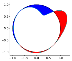
Figure 4: Deformation of the Fermi contour in two dimensional momentum space $\mathbf{p}/\pi$ for zero sound propagating along “cold spots” [22] diagonal $\beta=\pi/4$ in layered perovskites. For this special case of propagation along the nodal lines of the separable kernel of interaction, the electric charge, spin and current oscillations are zero. Moreover, we have a shear deformation of the Fermi surface in momentum space.

For propagation of zero sound along other directions it is necessary to take into account the Coulomb repulsion and zero sound will behave partially as a plasmon in a layered structure. For a general review on plasmons in cuprate superconductors see Ref. [23].

IV Conclusion and discussion

We investigated the propagation of the zero sound in a class of layered transition metal perovskites involving a $s$-$d$ interaction. We started and focused our attention on the CuO₂ plane that is a well-studied system. We were able to compare BCS and Fermi liquid reductions of the Hamiltonian and as a property of CuO₂ plane these two model Hamiltonian coincided. Moreover, we studied the influence of the sign of $J_{sd}$ coupling. For anti-ferromagnetic sign we have tendency to superconductivity, while for ferromagnetic sign we expect zero sound to be observed.

Unfortunately at the moment, starting with a theoretical scheme, it is difficult to conclude in which layered compounds the zero sound will have the longest lasting propagation and what material is technologically suitable to produce a clean $ac$-surface. It is most likely that a thin layer geometry would provide a solution.

Owing to the research outlined throughout this paper we conclude: First of all, zero sound exists only when $J_{sd}$ is negative and the $s$-$d$ interaction has a ferromagnetic sign. However, the $s$-$d$ exchange can create superconductivity only for antiferromagnetic sign (positive $J_{sd}$) of the exchange interaction. We arrive to the conclusion that in the normal phase of high-$T_{c}$ cuprates propagation of zero sound is impossible. Zero sound for high-$T_{c}$ cuprates is a dissipation mode, but thermal excitation of all those modes creates intensive scattering and Ohmic resistivity due to the exchange interaction and this strong angular dependence of the scattering rate is the cause of so called “hot spots” phenomenologically postulated for the interpretation of the experimental data [24]. Here we wish to add that thermal fluctuations of plasmons could also contribute to the hot spots along the Fermi contour [23].

Thermally agitated plasmons are related to electron density fluctuations which create electron scattering and ohmic resistivity due to exchange interaction. However, not for all doping levels the cuprates are superconducting and we do not exclude $J_{sd}$ to change its sign for some compounds.

Our main motivation to write this paper is to attract the attention of experimentalists with appropriate samples at hand to probe the zero-sound propagation in the $ab$-plane of transition metal layered perovskites. If Angle Resolved Photoemission Spectroscopy (ARPES) data are available for these materials, hot spots along the Fermi contour or even smearing of this contour will be a significant hint for intensive $s$-$d$ exchange which can lead to propagation of zero sound. In normal metals, the anisotropy of the electron-electron interaction is not strong enough to ensure zero sound propagation, but for layered perovskites such a phenomenon is most likely to occur. Another hint for intensive $s$-$d$ exchange can come from band calculations, the hybridization is strongest if all those 3 levels: for transition ion 4$s$ and 3$d$ and $p$-states for the chalcogen are close to each other and we have almost a triple coincidence (full overlapping).

From the practical point of view, a possible route towards the excitation of the zero sound could be achieved by an intense perturbation from one side of a narrow strip, and detection on the opposite side of the sample. This, however is still a remote possibility.

Last but not least, already a half century ago different kinds of zero sound are extensively studied by theoretical means. This topic continues to attract a great deal of interest within the scientific community. Here we mention but a few papers that are somehow directly linked to our study. Recent considerations include the two-dimensional zero-sound [25] and shear [26] zero sound for $p$-type interaction [27], and we finally conclude that except for ³He thin films and even two dimensional structures with large exchange interaction with ferromagnetic sign soon will become an interesting object for realization of the old idea of Landau [1, 2].

In this paper we have devised the theoretical framework for the possible emergence of zero sound in some layered perovskites involving ferromagnetic $s$-$d$ exchange interaction. We will continue our effort to extend the investigation to other transition-metal compounds along with distinct geometries to put the test the plausibility of the present theory. From the experimental side we hope that the current technological progress would make it possible to synthesize appropriate compounds allowing for the propagation of zero sound.

References

• Landau [1956] L. D. Landau, The Theory of a Fermi Liquid, Sov. Phys. JETP 3, 920 (1956), ZhETF 30(6), 1058 Dec (1956), http://www.jetp.ras.ru/cgi-bin/r/index/r/30/6/p1058?a=list, (in Russian).
• Landau [1957] L. D. Landau, Oscillations in a Fermi Liquid, Sov. Phys. JETP 5, 101 (1957), ZhETF 32(1), 59 Dec (1957), http://www.jetp.ras.ru/cgi-bin/r/index/r/32/1/p59?a=list, (in Russian).
• Keen et al. [1965] B. E. Keen, P. W. Matthews, J. Wilks, and B. Bleaney, The acoustic impedance of liquid helium-3, Proc. R. Soc. A: Math. Phys. Eng. Sci. 284, 125 (1965).
• Abel et al. [1966] W. R. Abel, A. C. Anderson, and J. C. Wheatley, Propagation of Zero Sound in Liquid ${\mathrm{He}}^{3}$ at Low Temperatures, Phys. Rev. Lett. 17, 74 (1966).
• Mishonov et al. [2022a] T. M. Mishonov, N. I. Zahariev, H. Chamati, and A. M. Varonov, Possible zero sound in layered perovskites with ferromagnetic $s$-$d$ exchange interaction, SN Appl. Sci. 4, 228 (2022a).
• Fukuda et al. [1996] T. Fukuda, Y. Endoh, K. Yamada, M. Takeda, S. Itoh, M. Arai, and T. Otomo, Dynamical Magnetic Structure of the Spin Density Wave State in Cr, J. Phys. Soc. Jpn. 65, 1418 (1996).
• Endoh et al. [1997] Y. Endoh, T. Fukuda, K. Nakajima, and K. Kakurai, Polarized Neutron Studies for Cr Excitations, J. Phys. Soc. Jpn. 66, 1615 (1997).
• Fuseya et al. [2000] Y. Fuseya, H. Maebashi, S. Yotsuhashi, and K. Miyake, Anomalous Fermi Liquid Effects in Two-Dimensional Hubbard Model near Half-Filling, J. Phys. Soc. Jpn. 69, 2158 (2000).
• Tsuruta et al. [2010] A. Tsuruta, K. Hattori, R. Ohta, and K. Miyake, Zero Spin Sound in Antiferromagnetic Metals: Case of Two-Dimensional t–t’ Hubbard Model, J. Phys. Soc. Jpn. 79, 084710 (2010).
• Lifshitz and Pitaevskii [1980a] E. M. Lifshitz and L. P. Pitaevskii, Statistical Physics. Part 2, Landau-Lifshitz course of theoretical physics, Vol. 9 (Pergamon, New York, 1980).
• Schubin and Wonsowsky [1934] S. Schubin and S. Wonsowsky, On the electron theory of metals, Proc. R. Soc. London, Ser. A 145, 159 (1934).
• Zener [1951a] C. Zener, Interaction Between the $d$ Shells in the Transition Metals, Phys. Rev. 81, 440 (1951a).
• Zener [1951b] C. Zener, Interaction between the $d$-Shells in the Transition Metals. II. Ferromagnetic Compounds of Manganese with Perovskite Structure, Phys. Rev. 82, 403 (1951b).
• Zener [1951c] C. Zener, Interaction between the $d$-Shells in the Transition Metals. III. Calculation of the Weiss Factors in Fe, Co, and Ni, Phys. Rev. 83, 299 (1951c).
• Kondo [1966] J. Kondo, Anomalous Scattering Due to s‐d Interaction, J. Appl. Phys. 37, 1177 (1966).
• Abrikosov [1988] A. A. Abrikosov, Fundamentals of the Theory of Metals (North Holland, Amsterdam, 1988).
• Mishonov and Penev [2010] T. M. Mishonov and E. S. Penev, Theory of High Temperature Superconductivity. A Conventional Approach (World Scientific, New Jersey, 2010).
• Nozières and Pines [1966] P. Nozières and D. Pines, The Theory of Quantum Liquids, 1st ed. (CRC Press, Boca Raton, 1966).
• Abrikosov et al. [1963] A. A. Abrikosov, L. P. Gor’kov, and I. Y. Dzyaloshinskii, Methods of quantum field theory in statistical physics (Prentice Hall, Englewood Cliffs, N.J., 1963).
• Lifshitz and Pitaevskii [1980b] E. M. Lifshitz and L. P. Pitaevskii, Physical Kinetics, Landau-Lifshitz course of theoretical physics, Vol. 10 (Pergamon, New York, 1980).
• Mishonov et al. [2022b] T. M. Mishonov, N. I. Zahariev, H. Chamati, and A. M. Varonov, Hot spots along the Fermi contour of high-$T_{c}$ cuprates explained by $s$-$d$ exchange interaction, SN Appl. Sci. 4, 242 (2022b).
• Ioffe and Millis [1998] L. B. Ioffe and A. J. Millis, Zone-diagonal-dominated transport in high-${T}_{c}$ cuprates, Phys. Rev. B 58, 11631 (1998).
• Greco et al. [2019] A. Greco, H. Yamase, and M. Bejas, Origin of high-energy charge excitations observed by resonant inelastic X-ray scattering in cuprate superconductors, Commun. Phys. 2, 3 (2019).
• Hlubina and Rice [1995] R. Hlubina and T. M. Rice, Resistivity as a function of temperature for models with hot spots on the Fermi surface, Phys. Rev. B 51, 9253 (1995).
• Khoo and Villadiego [2019] J. Y. Khoo and I. S. Villadiego, Shear sound of two-dimensional Fermi liquids, Phys. Rev. B 99, 075434 (2019)arXiv:1806.04157 [cond-mat.str-el] .
• Valentinis et al. [2021] D. Valentinis, J. Zaanen, and D. van der Marel, Propagation of shear stress in strongly interacting metallic Fermi liquids enhances transmission of terahertz radiation, Sci. Rep. 11, 7105:13 (2021).
• Ding and Zhang [2019] S. Ding and S. Zhang, Fermi-Liquid Description of a Single-Component Fermi Gas with $p$-Wave Interactions, Phys. Rev. Lett. 123, 070404 (2019).
• Valentinis [2021] D. Valentinis, Optical signatures of shear collective modes in strongly interacting Fermi liquids, Phys. Rev. Research 3, 023076 (2021).
• Valentinis et al. [2022] D. Valentinis, G. Baker, D. A. Bonn, and J. Schmalian, Kinetic theory of the non-local electrodynamic response in anisotropic metals: skin effect in 2D systems (2022), arXiv:2204.13344 [cond-mat.str-el] .
• Baker et al. [2022] G. Baker, T. W. Branch, J. Day, D. Valentinis, M. Oudah, P. McGuinness, S. Khim, P. Surówka, R. Moessner, J. Schmalian, A. P. Mackenzie, and D. A. Bonn, Non-local microwave electrodynamics in ultra-pure PdCoO2 (2022), arXiv:2204.14239 [cond-mat.mes-hall] .