Hot spots along the Fermi contour of high-$T_{c}$ cuprates analyzed by s-d exchange interaction

Abstract

We perform a thorough theoretical study of the electron properties of a generic CuO₂ plane in the framework of Shubin-Kondo-Zener s-d exchange interaction that simultaneously describes the correlation between T$\!{}_{c}$ and the Cu4s energy. To this end, we apply the Pokrovsky theory [J. Exp. Theor. Phys. 13, 447-450 (1961)] for anisotropic gap BCS superconductors. It takes into account the thermodynamic fluctuations of the electric field in the dielectric direction perpendicular to the conducting layers. We microscopically derive a multiplicatively separable kernel able to describe the scattering rate in the momentum space, as well as the superconducting gap anisotropy within the BCS theory. These findings may be traced back to the fact that both the Fermi liquid and the BCS reductions lead to one and the same reduced Hamiltonian involving a separable interaction, such that a strong electron scattering corresponds to a strong superconducting gap and vice versa. Moreover, the superconducting gap and the scattering rate vanish simultaneously along the diagonals of the Brillouin zone. We would like to stress that our theoretical study reproduces the phenomenological analysis of other authors aiming at describing Angle Resolved Photoemission Spectroscopy measurements. Within standard approximations one and the same s-d exchange Hamiltonian describes gap anisotropy of the superconducting phase and the anisotropy of scattering rate of charge carriers in the normal phase.

I Introduction

Since the discovery of high temperature superconductivity, the cuprates are one of the most studied materials. Nevertheless, the theoretical challenge to predict the critical temperature, say $T_{c}$, of certain materials still remains open [1] despite the significant number of theoretical studies on this topic. The purpose of our work is to give a microscopic explanation of hot/cold spots phenomenology [3, 4] of the normal phase of the optimally and over doped cuprates using Shubin-Kondo-Zener s-d exchange interaction in the CuO₂ which allows to explain $T_{c}$–Cu$4s$ energy correlation [5]. Hot spots are the regions with strong scattering and short lifetime, while cold spots are the regions with the longest lifetime or the weakest scattering. Röhler [6] noted that the Cu$4s$-3$d_{x^{2}-y^{2}}$ hybridization seems to be the crucial quantum chemical parameter controlling related electronic degree of freedom. For optimally doped and overdoped cuprates the used LCAO (linear combination of atomic orbitals) approximation for the electron bands [7] agrees with Local Density Approximation (LDA) band calculations [8, 9] and Angle Resolved Photoemission Spectroscopy (ARPES) measurements [10, 11]. The named experiments on optimally doped cuprates demonstrated that for momenta parallel to $(\pi,\,\pi)$, the electron spectral function exhibits a reasonably well defined quasiparticle peak, suggesting relatively weak scattering.

In this paper, we provide a microscopic derivation of this phenomenology devised in Refs. [3, 4]. The best conditions for the applicability of this phenomenology are satisfied for optimally and overdoped systems of layered cuprates. To achieve our task, we use the life-time $\tau_{\mathbf{p}}$, mean free path $l_{\mathbf{p}}$, and other quantities of the kinetics of the normal phase when we describe a normal metal. This is the case of optimally and overdoped cuprates far from Mott [12] metal-insulator transition and negligible, if any, pseudogap. In short, hot/cold spot phenomenology is applicable roughly speaking when cuprates exhibit a Fermi liquid behavior. Then, we can apply a standard set of notions for normal metals [13]. There is an emerging consensus that high-$T_{c}$ superconductivity is generated by an exchange interaction and in Section II, we introduce the simplest exchange interaction compatible with the gap anisotropy. In Section III, we briefly present the theoretical details, notations and notions of the s-d exchange interaction following Ref. [7]. ARPES experiments measure hot and cold spots regions accurately as it is shown in Section IV.

II The $s$-$d$ LCAO Hamiltonian

We start with the Linear Combination of Atomic Orbitals (LCAO) Hamiltonian [7, Eqs. (1.2), (2.9) and Figs. 1.1, 2.1]

$$\hat{H}^{\prime}= \sum_{\mathbf{n},\alpha}\left\{\hat{D}_{\mathbf{n},\alpha}^{\dagger}\left[(\epsilon_{d}-\mu)\hat{D}_{\mathbf{n},\alpha}\right.\right.$$

$$\left.-t_{pd}\left(-\hat{X}_{\mathbf{n},\alpha}+\hat{X}_{x-1,y,\alpha}+\hat{Y}_{\mathbf{n},\alpha}-\hat{Y}_{x,y-1,\alpha}\right)\right]$$

$$+\hat{S}_{\mathbf{n},\alpha}^{\dagger}\left[\left(\epsilon_{s}-\mu\right)\hat{S}_{\mathbf{n},\alpha}\right.$$

$$-t_{sp}\left.\left(-\hat{X}_{\mathbf{n},\alpha}+\hat{X}_{x-1,y,\alpha}-\hat{Y}_{\mathbf{n},\alpha}+\hat{Y}_{x,y-1,\alpha}\right)\right]$$

$$+\hat{X}_{\mathbf{n},\alpha}^{\dagger}[-t_{sp}(-\hat{S}_{\mathbf{n},\alpha}+\hat{S}_{x+1,y,\alpha})$$

$$-t_{pp}(\hat{Y}_{\mathbf{n},\alpha}-\hat{Y}_{x+1,y,\alpha}-\hat{Y}_{x,y-1,\alpha}+\hat{Y}_{x+1,y-1,\alpha})$$

$$-t_{pd}(-\hat{D}_{\mathbf{n},\alpha}+\hat{D}_{x+1,y,\alpha})+(\epsilon_{\mathrm{p}}-\mu)\hat{X}_{\mathbf{n},\alpha}]$$

$$+\hat{Y}_{\mathbf{n},\alpha}^{\dagger}[-t_{sp}(-\hat{S}_{\mathbf{n},\alpha}+\hat{S}_{x,y+1,\alpha})$$

$$-t_{pp}(\hat{X}_{\mathbf{n},\alpha}-\hat{X}_{x-1,y,\alpha}-\hat{X}_{x,y+1,\alpha}+\hat{X}_{x-1,y+1,\alpha})$$

$$-t_{pd}(\hat{D}_{\mathbf{n},\alpha}-\hat{D}_{x,y+1,\alpha})+(\epsilon_{\mathrm{p}}-\mu)\hat{Y}_{\mathbf{n},\alpha}]$$

$$-J_{sd}\sum_{\beta}\left.\hat{S}_{\mathbf{n},\beta}^{\dagger}\hat{D}_{\mathbf{n},\alpha}^{\dagger}\hat{S}_{\mathbf{n},\alpha}\hat{D}_{\mathbf{n},\beta}\right\},$$ (1)

where $\hat{S}_{\mathbf{n},\alpha}$, $\hat{D}_{\mathbf{n},\alpha}$, $\hat{X}_{\mathbf{n},\alpha}$, and $\hat{Y}_{\mathbf{n},\alpha}$ are Fermi annihilation operators at site or unit cell $\mathbf{n}=(x,y)$, $x,\,y=0,\pm 1,\pm 2,\pm 3,\dots$ of the CuO₂ lattice, $\mu$ is the chemical potential, $\alpha$ and $\beta$ are spin indices. and $J_{sd}$ is the anti-ferromagnetic Shubin-Zener-Kondo exchange amplitude. For the operator of electron number analogously we have

$$\hat{N}=-\partial_{\mu}\hat{H}^{\prime}.$$ (2)

We would like to point out that the LCAO approach is suitable tool to treat the Mott metal-insulator transition, see e.g. Ref. [14] and references therein.

In momentum representation

$$\hat{\Psi}_{\mathbf{n},\alpha}\equiv\begin{pmatrix}\hat{D}_{\mathbf{n},\alpha}\\ \hat{S}_{\mathbf{n},\alpha}\\ \hat{X}_{\mathbf{n},\alpha}\\ \hat{Y}_{\mathbf{n},\alpha}\end{pmatrix}\!=\!\frac{1}{\sqrt{N}}\sum_{\mathrm{b},\mathbf{p}}\mathrm{e}^{\mathrm{i}\mathbf{p}\cdot\mathrm{n}}\begin{pmatrix}D_{\mathrm{b},\mathbf{p}}\\ S_{\mathrm{b},\mathbf{p}}\\ \mathrm{e}^{\mathrm{i}\varphi_{x}}X_{\mathrm{b},\mathbf{p}}\\ \mathrm{e}^{\mathrm{i}\varphi_{y}}Y_{\mathrm{b},\mathbf{p}}\end{pmatrix}\hat{c}_{\mathrm{b},\mathbf{p},\alpha}$$ (3)

where the phases

$$\mathrm{e}^{\mathrm{i}\varphi_{x}}=\mathrm{e}^{\mathrm{i}p_{x}/2},\qquad\mathrm{e}^{\mathrm{i}\varphi_{y}}=\mathrm{e}^{\mathrm{i}p_{y}/2}$$ (4)

are chosen to provide real values for the eigenfunctions of Hamiltonian (1) in real space representation. Further, we will omit details of the standard substitution of the plane waves (3). From the technical point of view, we obtain sums over the different momenta with conserved total one

$$\sum_{\begin{subarray}{c}\mathbf{p}^{\prime},\,\mathbf{q}^{\prime},\,\mathbf{p},\,\mathbf{q}\\ \alpha,\,\beta\end{subarray}}\!\!\!\delta_{\mathbf{p}^{\prime}+\mathbf{q}^{\prime},\,\mathbf{p}+\mathbf{q}}\,S_{\mathbf{q}^{\prime}}D_{\mathbf{p}^{\prime}}\langle{\color[rgb]{0,0,0}\hat{c}^{\dagger}_{\mathbf{q}^{\prime}\beta}\hat{c}^{\dagger}_{\mathbf{p}^{\prime}\alpha}}{\color[rgb]{0,0,0}\hat{c}_{\mathbf{p}\alpha}\hat{c}_{\mathbf{q}\beta}}\rangle S_{\mathbf{p}}D_{\mathbf{q}}.$$ (5)

The BCS reduction of the Hamiltonian requires to take into account only annihilation operators with opposite momenta and simultaneously in self-consistent approximation to approximate the averaged product of creation and annihilation operators with the product of averaged two creation and two annihilation operators

$$\delta_{\mathbf{p}^{\prime}+\mathbf{q}^{\prime},\,\mathbf{p}+\mathbf{q}}\,S_{\mathbf{q}^{\prime}}D_{\mathbf{p}^{\prime}}\langle{\color[rgb]{0,0,1}\hat{c}^{\dagger}_{\mathbf{q}^{\prime}\beta}\hat{c}^{\dagger}_{\mathbf{p}^{\prime}\alpha}}{\color[rgb]{1,0,0}\hat{c}_{\mathbf{p}\alpha}\hat{c}_{\mathbf{q}\beta}}\rangle S_{\mathbf{p}}D_{\mathbf{q}}$$

$$\approx\delta_{\mathbf{q}^{\prime}+\mathbf{p}^{\prime},0}\,\delta_{\mathbf{q}+\mathbf{p},0}\,\chi_{\mathbf{p}^{\prime}}\langle{\color[rgb]{0,0,1}\hat{c}^{\dagger}_{-\mathbf{p}^{\prime}\overline{\alpha}}\hat{c}^{\dagger}_{\mathbf{p}^{\prime}\alpha}}\rangle\langle{\color[rgb]{1,0,0}\hat{c}_{\mathbf{p}\alpha}\hat{c}_{-\mathbf{p}\overline{\alpha}}}\rangle\chi_{\mathbf{p}}$$

Additionally in these anomalous averages, we have to perform a Fermi liquid (FL) reduction

$$\delta_{\mathbf{p}^{\prime}+\mathbf{q}^{\prime},\,\mathbf{p}+\mathbf{q}}\,S_{\mathbf{q}^{\prime}}D_{\mathbf{p}^{\prime}}\langle{\color[rgb]{1,0,0}\hat{c}^{\dagger}_{\mathbf{q}^{\prime}\beta}}{\color[rgb]{0,0,1}\hat{c}^{\dagger}_{\mathbf{p}^{\prime}\alpha}\hat{c}_{\mathbf{p}\alpha}}{\color[rgb]{1,0,0}\hat{c}_{\mathbf{q}\beta}}\rangle S_{\mathbf{p}}D_{\mathbf{q}}$$

$$\approx\delta_{\mathbf{q}^{\prime},\mathbf{q}}\,\delta_{\mathbf{p}^{\prime},\mathbf{p}}\,\chi_{\mathbf{p}}\langle{\color[rgb]{0,0,1}\hat{c}^{\dagger}_{\mathbf{p}^{\prime}\alpha}\hat{c}_{\mathbf{p}\alpha}}\rangle\langle{\color[rgb]{1,0,0}\hat{c}^{\dagger}_{\mathbf{q}^{\prime}\beta}}{\color[rgb]{1,0,0}\hat{c}_{\mathbf{q}\beta}}\rangle\chi_{\mathbf{q}}$$

where

$$\chi_{\mathbf{p}}\equiv S_{\mathbf{p}}D_{\mathbf{p}},\qquad S_{\mathbf{p}}=S_{-\mathbf{p}}.$$ (6)

One of the main result we report here is the coincidence of BCS [7] and FL multiplicatively separable kernels of the reduced Hamiltonians. Moreover, two fermion operators in averaging brackets have to be considered as averaged number of particles.

III Notions and notations

The critical temperature $T_{c}$ and the superconducting gap $\Delta$ are calculated within the standard BCS approach

$$2J_{sd}\,\int_{0}^{2\pi}\int_{0}^{2\pi}\frac{\chi_{\mathbf{p}}^{2}}{2E_{\mathbf{p}}}\tanh\left(\frac{E_{\mathbf{p}}}{2T}\right)\frac{\mathrm{d}p_{x}\mathrm{d}p_{y}}{(2\pi)^{2}}=1,$$ (7)

with

$$E_{\mathbf{p}}\equiv \ \sqrt{\eta_{\mathbf{p}}^{2}+\Delta_{\mathbf{p}}^{2}},$$

$$\eta_{\mathbf{p}}\equiv \epsilon_{\mathbf{p}}-\epsilon_{\mathrm{{}_{F}}},\qquad\Delta_{\mathbf{p}}=\Xi(T)\,\chi_{\mathbf{p}},$$

where $\Xi(T)$ is the superconducting order parameter, $\epsilon_{\mathbf{p}}$ is energy of the conduction band, which obeys the secular equation

$$\mathcal{A}xy+\mathcal{B}(x+y)+\mathcal{C}=0.$$ (8)

Here, we have introduced

$$x=\sin^{2}\left(\frac{p_{x}}{2}\right),\qquad y=\sin^{2}\left(\frac{p_{y}}{2}\right)$$ (9)

and

$$\mathcal{A}\left(\epsilon\right) =32\tau_{sp}^{2}\left(2t_{pd}^{2}+t_{pp}\varepsilon_{d}\right),\quad\tau_{sp}^{2}=t_{sp}^{2}-\frac{1}{2}\varepsilon_{s}t_{pp},\$$

$$\mathcal{B}(\epsilon) =-4\varepsilon_{\mathrm{p}}(t_{sp}^{2}\varepsilon_{d}+t_{pd}^{2}\varepsilon_{s}),$$

$$\mathcal{C}(\epsilon) =\varepsilon_{d}\varepsilon_{s}\varepsilon_{\mathrm{p}}^{2},$$

with $\varepsilon_{s}=\epsilon-\epsilon_{s}$, $\varepsilon_{d}=\epsilon-\epsilon_{d}$, $\varepsilon_{\mathrm{p}}=\epsilon-\epsilon_{\mathrm{p}}$. The main detail of the LCAO-$J_{sd}$ theory for the electron processes in CuO₂ plane is the function $\chi_{\mathbf{p}}$, the separable exchange interaction

$$\chi_{\mathbf{p}}= \;S_{\mathbf{p}}D_{\mathbf{p}}=4\varepsilon_{\mathrm{p}}t_{sp}t_{pd}(x-y)$$

$$\times\left[\varepsilon_{s}\varepsilon_{\mathrm{p}}^{2}-4\varepsilon_{\mathrm{p}}t_{sp}^{2}\,(x+y)+32t_{pp}\tau_{sp}^{2}\,xy\right]$$

$$\times\left\{\left[4\varepsilon_{\mathrm{p}}t_{sp}t_{pd}\,(x-y)\right]^{2}\right.$$

$$\qquad+\left[\varepsilon_{s}\varepsilon_{\mathrm{p}}^{2}-4\varepsilon_{\mathrm{p}}t_{sp}^{2}\,(x+y)+32t_{pp}\tau_{sp}^{2}\,xy\right]^{2}$$

$$\qquad+4x\left[(\varepsilon_{s}\varepsilon_{\mathrm{p}}-8\tau_{sp}^{2}y)t_{pd}\right]^{2}$$

$$\qquad\left.+4y\left[(\varepsilon_{s}\varepsilon_{\mathrm{p}}-8\tau_{sp}^{2}x)t_{pd}\right]^{2}\right\}^{-1},$$ (10)

where $S_{\mathbf{p}}$ and $D_{\mathbf{p}}$ are the amplitudes for the band electron to be in the Cu4$s$ and Cu3$d_{x^{2}-y^{2}}$ orbitals, respectively. In other words, $\chi(p_{x},p_{y})$ is the magnitude of s-d hybridization, the main ingredient of the matrix elements of s-d exchange interaction. This hybridization amplitude $\chi_{\mathbf{p}}$ enters into the interaction kernel

$$f(\mathbf{p},\mathbf{q})\equiv-2J_{sd}\chi_{\mathbf{p}}\chi_{\mathbf{q}}$$ (11)

which is one and the same in the BCS and Fermi liquid reductions of the exchange s-d Hamiltonian. Let us note that this result is corroborated by the proof of Pokrovsky [15, 16] that in the weak coupling limit of the BCS theory any arbitrary pairing can be approximated by a separable kernel. In this case $\chi_{\mathbf{p}}$ is the eigenfunction of the pairing kernel corresponding to maximal in modulus eigenvalue. For more computational details the interested reader may consult an unabridged version of the present study [17]. In the following we give a microscopic explanation of the hot spots observed by ARPES experiments and postulated phenomenologically in Refs. [3, 4]. In some sense this is a hint for the importance of the s-d exchange interaction in shaping the electronic properties of the CuO₂ plane. Now we are in position to address analytically the gap anisotropy and the kinetics of the normal phase that has been postulated in the past. We will present some results of the self-consistent treatment of this $J_{sd}\,$-LCAO Hamiltonian (1) and compare to ARPES data.

Before proceeding further with our analysis, we would like to point out that the “Tight binding” and “LCAO” methods are to some extent equivalent. Generally, the tight binding method is mainly used in a more mathematical physics context, while LCAO suggests that the parameters of the lattice Hamiltonian could be evaluated starting from the atomic structure and the corresponding wave functions. For example, the transfer (or hopping integrals) $t_{pp}$, $t_{pd}$ and $t_{sp}$ can be evaluated as surface integrals of the wave functions of neighboring atoms. The corresponding problem for H${}_{2}^{+}$ ion is provided in many textbooks on quantum mechanics, for example see Ref. [18]. Following the same reasoning, we obtain for the Hubbard $U$ integral

$$U_{dd} =\left\langle\frac{e^{2}}{r_{12}}\right\rangle$$

$$=\iint\frac{e^{2}}{r_{12}}\left|\psi_{\mathrm{Cu}3d}\left(\mathbf{r}_{1}\right)\right|^{2}\left|\psi_{\mathrm{Cu}3d}\left(\mathbf{r}_{2}\right)\right|^{2}\mathrm{d}^{3}\mathbf{r}_{1}\mathrm{d}^{3}\mathbf{r}_{2}$$

describing the Coulomb repulsion of two electrons in one Cu atom [12, Eq. (19), page 81]. As the Cu3$d$ orbital is the closest of all orbitals to the nucleus from the 4 band LCAO model, the corresponding $U_{dd}$ integral is the largest. In brief, the lattice Hamiltonian accounts for the atomic structure via the atomic wave functions. This trivial consideration above is readily applied to the Mott transition or charge transfer Mott transition, as well as the role of the exchange interaction are discussed very recently in Ref. [19]. The use of LCAO for Mott transition and related topics is known for at least half a century, see e.g. the monograph by Mott  [12, Eq. (10), p. 9; Eq. (12), p. 12, Eq. (26), p. 25; Eq. (19), p. 81, Eq. (24), p. 100, Eq. (40), p. 116, p. 129] on metal-insulator transitions. Last but not least, the Mott transition is not closely related to our present study. Hot/cold spots and BCS approach are better applicable to over-doped cuprates, which are more or less normal metals.

IV Results

The performed calculations in the framework of the derived s-d LCAO Hamiltonian were performed with values of the single site energies $\epsilon_{d}=0$ eV, $\epsilon_{p}=-0.9$ eV, $\epsilon_{s}=4.0$ eV and the hopping integrals $t_{sp}=2.0$ eV, $t_{pd}=1.5$ eV [8, 5], $t_{pp}=0.2$ eV [20]. The in-plane lattice constant $a_{0}=3.6$ Å, while the filling factor $f_{h}=0.58$ is chosen to correspond to the optimally hole doped cuprates. Before addressing our final purpose of hot/cold spots of layered cuprates, we rederive some well-known results for their superconducting properties. In order to explain the normal state phenomenology, we use the s-d exchange model that is able to provide an adequate explanation of the gap symmetry and the anisotropy.

IV.1 Evaluation of the critical temperature $T_{c}$

The remarkable correlation between the critical temperature $T_{c}$ and the electronic parameter $r$ [5] covers the whole temperature range of cuprate high-$T_{c}$ superconductivity and its explanation is an indispensable ingredient of the theory of high-$T_{c}$ superconductivity. The dimensionless parameter is defined by [5]

$$r\equiv\frac{1}{2(1+s)},\quad s(\epsilon_{\mathrm{{}_{F}}})\equiv\dfrac{(\epsilon_{s}-\epsilon_{\mathrm{{}_{F}}})(\epsilon_{\mathrm{{}_{F}}}-\epsilon_{\mathrm{p}})}{(2t_{sp})^{2}}.$$ (12)

Here $\epsilon_{s}$, $\epsilon_{d}$, and $\epsilon_{\mathrm{p}}$ are single site energies for Cu4$s$, Cu3$d_{x^{2}-y^{2}}$ and O2$p$ atomic levels, and $\epsilon_{\mathrm{{}_{F}}}$ is the Fermi energy. Following Ref. [5] the transfer integrals between these four atomic orbitals are denoted by $t_{pd}$, $t_{sp}$, $t_{pp}$.

The $r$-$T_{c}$ correlation for the Hamiltonian (1) compared to some experimental studies taken from Ref. [5] is depicted in Fig. 1. The continuous line in Fig. 1 is the result of our calculations according to the gap equation (7) supposing that $J_{sd}$ is approximately the same for all layered cuprates at a fixed set of LCAO parameters. Then for a fixed value of $J_{sd}$ varying only Cu4$s$ level $\epsilon_{s}$ we calculated $T_{c}$ from the same equation (7). For some novel materials the $\epsilon_{s}$ parameter is determined by fitting the Fermi contour at fixed other parameters and then the parameter $r$ is calculated according to (12). This is an acceptable approximation since $T_{c}$ and the shape of the Fermi contour are very sensitive to $\epsilon_{s}$ as pointed out in Ref. [5].

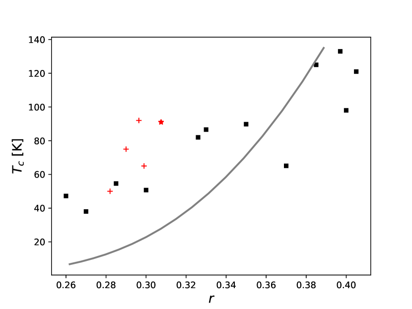
Figure 1: Correlation between the $r$ parameter and $T_{c}$: ($\blacksquare$) Pavarini et al. [5, Fig. 5], (+) Vishik et al. [21] for underdoped cuprates, ($\mathbf{\star}$) Kaminski et al. [22] and Zonno et al. [23] from ARPES data; the solid line [24] is our traditional BCS interpretation for s-d exchange amplitude $J_{sd}$ approximately equal for all cuprates, which is a fitting parameter of the theory and can be used to determine the intensity of the scattering rate in the normal phase. The value of $J_{sd}$ used to obtain the curve in the figure is 7.23 eV.

The band-structure correlations between the shape of the Fermi contour and the critical temperature for optimally hole doped cuprates reveal two important conclusions: 1) we have a usual metal with single conduction band or 2) the electron conductivity is determined by a lower Hubbard band, and the Fermi operator approximation provides a satisfactory accuracy to be included in the standard BCS scheme. The $d$-wave superconducting gap was also confirmed by ARPES measurements, see Damascelli et. al. [25, V. Superconducting Gap, Figs. 46, 50] and references therein. High-$T_{c}$ cuprates are doped Mott insulators, but as it was pointed out by Lee, Nagaosa and Wen [26]: beyond optimal doping (called the overdoped region), the normal metal properties gradually reappear. Just in this region the hot/cold spots phenomenology [3, 4] and the $r$–$T_{c}$ correlation are both applicable, which allows BCS treatment. Recently Lee, Kivelson and Kim [27] used Bogolyubov-de Gennes BCS approach to analyse cold spots and glassy nematicity in underdoped cuprates. This significantly extends the hot/cold spots phenomenology for cuprates; it seems that the underdoped regime requires to take into account more parameters in comparison to the simple BCS picture of the overdoped regime. That is why we have included the experimental data for underdoped cuprates in Fig. 1 to the band trend of the model under consideration. The authors of Ref. [27] show the existence of glassy charge order in the pseudogap phase of HTS cuprates. Momentum and real space probes show charge density wave (CDW) order with moderate finite correlation length. Results from diffraction, local probes, and transport suggest nematic order. Most of the theory has focused on long-range ordered states, or dynamically fluctuating order parameter. Whereas glass order implies short-range heterogeneities. The authors concluded that the self-consistent BCS approach is an acceptable approximation for the study of many characteristics of underdoped cuprates.

Electron band calculations of Fermi surfaces (contours) of the cuprates perfectly describe the experimentally observed ARPES Fermi contours, while the realistic LCAO approximation of the ab initio bands are not that accurate, since they neglect correlations. Moreover in Hubbard model description of the electron structure the ratio of $t$-$t^{\prime}$ parameters is taken from electron band calculations. In any case the Cu4$s$ energy $\epsilon_{s}$ is included in a unique way in the LCAO approximation of the band structure.

Let us recall the $J_{sd}$ exchange interaction is widely used to explore the magnetism in d-metals, such as transition metals and their compounds. In the present study, we have solved the corresponding integral equations and have found that the $J_{pd}$ exchange amplitude gives a gap anisotropy and hot/cold spots that do not agree with the experimental data. It was shown [28, 29, 30] that the matrix elements of the $J_{pd}$ pairing added to the $J_{sd}$ pairing contribute only a de-pairing perturbation. In this way the experimental data determine which exchange amplitude is dominant. In short, if we account for $J_{pd}$ or $J_{ps}$ in the BCS gap equation the solution will possess again a crystal symmetry albeit a different one.

IV.2 From the Hubbard repulsion to the $s$-$d$ anti-ferromagnetic exchange interaction

It is obvious that hybridization is a one body problem, yet to determine the hybridization amplitude $\chi_{\mathbf{p}}$ it is necessary to compute the matrix elements of the exchange interaction. The s-d exchange interaction was proposed eighty years ago but up to date there are no reliable formulas for the calculation of the exchange amplitude $J_{\mathrm{sd}}$ that is a parameter of the theory. The exchange amplitudes defining the physics of high-$T_{c}$ superconductors are also parameters of the theory. To show that $J_{\mathrm{sd}}$ is anti-ferromagnetic in nature, we start with the well-known microscopic formula, see e.g. Ref. [31, Eq. (7.17)] and the more recent textbook [32],

$$J= 2\left|V_{0\mathbf{k}_{{}_{\mathrm{F}}}}\right|^{2}\frac{U}{E_{0}(E_{0}+U)}$$

$$\rightarrow-J_{sd}\simeq 2\left|t_{pd}\right|^{2}\frac{U_{dd}}{(\epsilon_{d}-\epsilon_{\mathrm{{}_{F}}})[(\epsilon_{d}-\epsilon_{\mathrm{{}_{F}}})+U_{dd}]}.$$ (13)

Here we make some qualitative replacements: 1) the definition of the sign is a matter of convention, we use positive $J_{sd}$ corresponding to singlet pairing and a tendency to anti-ferromagnetism; 2) the Hubbard $U$ is actually the Coulomb interaction $U_{dd}$ when two electrons are simultaneously on Cu3$d_{x^{2}-y^{2}}$ state; 3) the amplitude of electron transfer between Kondo impurity $V_{0\mathbf{k}_{{}_{\mathrm{F}}}}$ and an electron on the Fermi surface is just the lattice transfer integral $t_{pd}$; 4) the electron energy on the Kondo impurity $E_{0}$ is according to our interpretation the energy level of the Cu3$d_{x^{2}-y^{2}}$ state $\epsilon_{d}$. For more details, we recommend the monograph by White and Geballe [31, Chap. 7, Sec. 1] and cited therein works by Anderson, Wolff, Schrieffer, and Wilson. To proceed further, we use the Single Impurity Anderson Model (SIAM) [33] for the virtual bound state in order to describe qualitatively the anti-ferromagnetism in the CuO₂ lattice, where each Cu ion is viewed as Kondo impurity. In short, this is not a proof but only a qualitative explanation why the phenomenology of the s-d interaction can be successful for a simultaneous description of the gap anisotropy and hot/cold phenomenology.

Nowadays it is known that the s-d four-fermion interaction explains fairly well the gap anisotropy in the overdoped cuprates [34, 35, 36, 37]. The study of the two-impurity Anderson model (TIAM) gives new insights showing that the anti-ferromagnetic contribution to $J_{\mathrm{RKKY}}$ is determined by $\left(t^{\mathrm{eff}}\right)^{2}/U$ where $U$ denotes the Coulomb interaction [34] and RKKY (Ruderman-Kittel-Kasuya-Yosida). The single-impurity problem was extended to lattice models [35], multi-impurity Anderson models and periodic Anderson models [36] and multi impurity arrays [37]. It would be interesting to explore this matter in CuO₂ to unveil the influence of strong electron correlations on electron-electron scattering for overdoped cuprates. In the next section we use the s-d exchange interaction to describe the anisotropy of the scattering rate in the normal phase of overdoped cuprates.

IV.3 Charge carriers scattering by density fluctuations. Who could be blind to the beauty of the blue sky?

One of the main properties of the high-$T_{c}$ cuprates is their strong electrodynamic anisotropy, they possess conducting $a$-$b$ planes and almost dielectric behavior in the $c$-direction perpendicular to CuO₂ planes. In the layered metal, the conducting CuO₂ layers (single or multiple) are separated by insulating layers. In some sense the $c$-direction perpendicular to the layers can be dubbed dielectric direction. Conducting layers (CuO₂)₂, double for YBa₂Cu₃O_7-δ and Bi₂Sr₂Ca₁Cu₂O₈, serve like plates of a plane capacitor. In 1907 Albert Einstein [38] pointed out that in a plane capacitor with a short circuit between its plates, thermodynamic fluctuations of the electric voltage between the plates is proportional to the thermal fluctuations of the electric field $E_{z}$ perpendicular to the plates

$$\frac{1}{2}CU^{2}=\frac{1}{2}T,\quad U=c_{0}E_{z},\quad C=\frac{\varepsilon_{0}b_{0}^{2}}{c_{0}},$$ (14)

where $b_{0}^{2}$ is the area of the plates and we qualitatively assume $b_{0}\sim a_{0}$ to be equal to the lattice constant, $c_{0}$ is the distance between conducting planes, and $\varepsilon_{0}=1/4\pi$ or in SI $\varepsilon_{0}=1/4\pi c^{2}\,10^{-7}$. Having a plane capacitor system, state-of-the-art statistical consideration requires the fluctuation of the electrical field $E_{z}$ to be taken into account. For a layered metal with weak coupling between layers, fluctuations of the transverse electric field have to be taken into account. On the other hand the thermodynamic fluctuations of the electric field are proportional to the thermodynamic fluctuation of the two dimensional electron density of metallic CuO₂ layers $q_{e}\,\delta n_{\mathrm{2D}}=\varepsilon_{0}E_{z}$. The thermodynamic fluctuations of two dimensional electron density $\delta n_{\mathrm{2D}}$ are a corner stone of the theory of Ohmic resistivity $\varrho$. We have strong pairing interaction in the superconducting phase, but what happens in the normal phase? A plane wave of charge carrier scatters off the density fluctuations by the exchange interaction. This is analogous to the Rayleigh scattering [39] of the sunlight in the Earth atmosphere [40]. Who could be blind to the blue sky [40]. In short, 2D electrons scatter off by the fluctuation of the 2D electron density. The linear dependence of the resistivity in the metallic $ab$-plane $\varrho_{ab}\propto T$ in this construction is just a demonstration of the classical fluctuation of the electric field $E_{z}$ in the dielectric $c$-direction. Statistics of waves scattered by thermal density fluctuations; we have common mechanism for the color of the blue sky and Ohmic resistance of the layered transition metal perovskites.

Let us mark some details of this chain of considerations [41, Eqs. (2.2) and (39.20)]: first we perform Fermi liquid reduction of the exchange Hamiltonian and the reduced Fermi liquid Hamiltonian $\hat{H}_{{}_{\mathrm{FL}}}$ determines the single particle spectrum

$$\varepsilon(\mathbf{p},\mathbf{r})= \epsilon_{\mathbf{p}}+\frac{\partial\hat{H}_{{}_{\mathrm{FL}}}}{\partial\hat{n}_{\mathbf{p},\alpha}}\rightarrow\ \epsilon_{\mathbf{p}}+\frac{1}{N}\sum_{\mathbf{q}.\beta}f(\mathbf{p},\mathbf{q})n_{\mathbf{q},\beta}(\mathbf{r})$$

$$= \epsilon_{\mathbf{p}}+\frac{(-2J_{sd})}{N}\chi_{\mathbf{p}}\sum_{\mathbf{q}}\chi_{\mathbf{q}}n_{\mathbf{q}}(\mathbf{r},t).$$ (15)

In the quasi-classical Wentzel-Kramers-Brillouin (WKB) approximation in the spectrum (15), we substitute the thermal fluctuations of the Fourier components $\delta n_{\mathbf{q}}$ of the 2D electron density proportional to the whole electron density at some space point $\mathbf{r}$ via

$$\frac{1}{N}\sum_{\mathbf{q}}\chi_{\mathbf{q}}\,\delta n_{\mathbf{q}}(\mathbf{r},t)\simeq\delta n(\mathbf{r}).$$ (16)

The thermodynamic fluctuations suggest that the dispersion of the 2D electron density is proportional to the temperature

$$\langle[\delta n(\mathbf{n})]^{2}\rangle\propto T.$$ (17)

Thus, using the space $\mathbf{r}$ dependent component of the Fermi liquid correction to the spectrum (15) as a random scattering potential with the aid of the second Fermi golden rule of the perturbation theory, we obtain scattering rate proportional to the temperature and square of the hybridization amplitude $\Gamma_{\mathbf{p}}\propto T\chi_{\mathbf{p}}^{2}$. As the s-d hybridization function may be approximated with an acceptable accuracy with a single sinusoidal, introducing $\tilde{\theta}=\theta-\tfrac{\pi}{2}$ for the angular dependence of the scattering rate

$$-\mathrm{Im}(\epsilon_{\mathbf{p}})\propto\Gamma_{\mathbf{p}} =\frac{\Gamma_{0}}{4}\sin^{2}(2\tilde{\theta})+\frac{1}{\tau_{0}}\approx\Gamma_{0}\tilde{\theta}^{2}+\frac{1}{\tau_{0}},$$

where $\Gamma_{0}=k_{1}T$, we obtain the results of the Ioffe and Millis phenomenology [4, Eqs. (4-5)]. Analyzing kinetics of the normal phase Ioffe and Millis [4] postulate a separable kernel [4, Eq. (22)] which naturally can be derived from the s-d interaction.

The idea of thermal fluctuations of the electric charge and the associated density fluctuations of the two dimensional charge carriers density can be most easily interpreted in terms of a plane capacitor model. Two layer unit cell cuprates have in this sense a plane capacitor performed by the double (CuO₂)₂ layer. However, even around a single CuO₂ plane thermal fluctuations of the electrostatic potential will be in some sense uniform. Every 2D fluctuating mode will have again $\frac{1}{2}T$ energy according to the equipartition theorem. The only condition for the applicability of the classical statistics is that the temperature should be higher than the typical frequency of the eigenmodes, but 2D plasmons are gapless. For thin films in the superconducting phase the plasmon frequency can be significantly smaller than the superconducting gap and temperature, as it was theoretically predicted [42] and later experimentally confirmed [43]. The idea that linear Ohmic thermal resistance can be created by thermal fluctuations of the electric potential may be exploited in many physical phenomena. Only the the corresponding electrostatic task will be slightly different. We conclude that it is praiseworthy to perform the relevant calculations to the specific system under consideration, here however, we continue with the simplest implementation of a plane capacitor. The comparison of the detailed electrostatic problem to experimentally observed Ohmic resistance can be considered as a final explanation of this long standing problem. Appropriate layered structures with single layer copper oxide planes are available for many years [44]. In the opposite case of perovskites with moderate anisotropy when $c$-polarized plasmons have frequency higher than the temperature the electric field-density fluctuations are frozen and Ohmic resistivity $\varrho_{ab}\propto T^{2}$ according to Baber [45], and Landau-Pomeranchuk [46] theory. For a qualitative consideration and state-of-the-art calculation see the monographs by Mott [12, page 72] and Lifshitz and Pitaevskii [41, Sec. 1] and [47, Sec. 75, 76].

IV.4 Some remarks on ARPES

Taking into account the thermodynamic fluctuations of $E_{z}$ according to the Herapath-Waterston equipartition theorem [48, 49, 50], we obtain that the resistivity is proportional to the temperature, i.e. $\varrho\propto T$. Formally, the scattering of the density fluctuations is described by an imaginary correction to the electron spectrum

$$\epsilon_{\mathbf{p}}\rightarrow\epsilon_{\mathbf{p}}=\Sigma^{\prime}(\mathbf{p},\omega)+\mathbf{i}\Sigma^{\prime\prime}(\mathbf{p},\omega),$$ (18)

where

$$-\Sigma^{\prime\prime}=\Gamma_{\mathbf{p}}=k_{1}T\,\frac{\Gamma_{0}}{4}\sin^{2}(2\tilde{\theta})+\frac{1}{\tau_{0}}.$$

Here we wish to recall the well-known relation between the Green function $G$ and the self-energy $\Sigma$, and the one particle spectral function $A$

$$G(\mathbf{p},\omega)=\frac{1}{\hbar\omega-\epsilon_{\mathbf{p}}-\Sigma}\,,$$

$$A(\mathbf{p},\omega)=-\frac{1}{\pi}\frac{\Sigma^{\prime\prime}}{[\hbar\omega-\epsilon_{\mathbf{p}}-\Sigma^{\prime}]^{2}+[\Sigma^{\prime\prime}]^{2}}\,,$$

$$\int_{-\infty}^{\infty}A(\mathbf{p},\omega)\mathrm{d}(\hbar\omega)=1,$$

see the well known monographs [41, Sec. 14 Self-energy function], [51, Sec. 10 Dyson equation] and the review [25, Eqs. (13-20)]. The Boltzmann equation approach does not require meticulously calculated spectral density $A(\mathbf{p},\omega)$, but only a simple analytical approximation for the imaginary component of the self-energy

$$\frac{1}{\tau_{\mathbf{p}}}=\Gamma_{\mathbf{p}}=Z_{\mathbf{p}}|\Sigma^{\prime\prime}|,\qquad Z_{\mathbf{p}}\leq 1.$$ (19)

For weak scattering of gas particles on static inhomogeneities the kinetic approach gives the Lorentzian approximation

$$A(\mathbf{p},\omega)=\frac{1}{\pi}\frac{\hbar/\tau_{\mathbf{p}}}{(\hbar\omega-\varepsilon_{\mathbf{p}})^{2}+(\hbar/\tau_{\mathbf{p}})^{2}}.$$ (20)

We recall the basic notion of electron spectra just to establish a bridge between the CuO₂ plane thermal fluctuations of the electric potential and ARPES spectra. An exact extraction of the width of the approximating Lorentzian from experimental data is far beyond the purpose of this initial study.

In the nice review by Lee, Nagaosa and Wen [26] on the physics of high-$T_{c}$ superconductors, such as doped Mott insulators, it is emphasized that the normal state of the optimally doped ones exhibits unusual properties. Linear in $T$ resistivity is quoted as a nice illustration of non-Fermi liquid behavior since the early days of high-$T_{c}$ superconductivity. We wish to comment that this relationship is valid even for optimal $T_{c}$, because this linearity is a simple proof of the applicability of the equipartition theorem for transverse electric field in layered metals. Nothing strange that statistical physics is applicable to a layered metal; this situation is known as “strange metal”, i.e. applicability of the Fermi liquid theory to layered metals. A non-Fermi liquid is just a layered Fermi gas with exchange interaction and electric field between the layers. This problem however is far from the linear resistivity solution explained by Rosch [52] as a property of nearly antiferromagnetic metals close to the quantum critical point. Later on Lee [53] showed that the low temperature $T$-linear resistivity may be traced back to umklapp scattering from a critical mode.

Concerning the applicability of the BCS theory to the high-$T_{c}$ superconductivity, we wish to stress that recently Lee, Kivelson and Kim [27] have used the de Gennes–Bogolyubov approach to explain cold-spots and glassy nematicity in underdoped cuprates. Comparing ARPES, scanning tunneling microscopy (STM) and optical measurements with their BCS calculations, they observe consonance between cold-spot of glassy nematics and the gap nodes of d-wave superconductivity. In the directions where the exchange interaction is zero, one may observe the small contribution of the Coulomb scattering by density fluctuations which is also $\propto T$. In such a way, following a chain of standard approximations and supposing that $\tau_{\mathrm{cold}}=\tau_{0}$, we arrive at the widely accepted anisotropy of the lifetime

$$\frac{1}{\tau(\theta)}=\frac{1}{\tau_{\mathrm{hot}}}\cos^{2}(2\theta)+\frac{1}{\tau_{\mathrm{cold}}}.$$ (21)

By introducing the averaged over the Fermi contour relaxation time

$$\tau_{\mathrm{Drude}}\equiv\ \langle\tau(\theta)\rangle=\int_{0}^{2\pi}\tau(\theta)\,\frac{\mathrm{d}\theta}{2\pi}$$

$$= \dfrac{1}{\sqrt{\dfrac{1}{\tau_{\mathrm{cold}}\tau_{\mathrm{hot}}}+\dfrac{1}{\tau_{\mathrm{cold}}^{2}}}}\approx\sqrt{\tau_{\mathrm{cold}}\tau_{\mathrm{hot}}}\gg\tau_{\mathrm{hot}},$$

the conductivity takes the standard Drude form

$$\sigma_{ab}=q_{e}^{2}n_{e}\frac{\tau_{\mathrm{Drude}}}{m_{c}},\qquad\frac{1}{\tau_{\mathrm{hot}}}\equiv\frac{\Gamma_{0}}{4},$$

where $m_{c}$ is the optical mass in CuO₂ plane; $\tau_{\mathrm{cold}}$ is created by the Coulomb scattering and the small $\tau_{\mathrm{hot}}$ by the exchange one. In order to check whether we are on the correct track we draw the hybridization probability $\chi_{\mathrm{p}}^{2}$ from Fig. 2 together with ARPES data for the width of the spectral lines in Fig. 3.

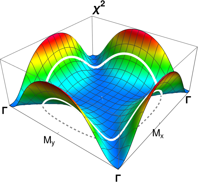
Figure 2: The hybridization probability $\chi_{\mathbf{p}}^{2}=S_{\mathbf{p}}^{2}D_{\mathbf{p}}^{2}$. Heights around the $M$ points correspond to hot spots, while the navigation channels in the deep blue sea along the diagonals between the $\Gamma$ points correspond to cold spots in agreement with both Refs. [3, 4]. Fermi contour (dotted line) is projected on the $\chi_{\mathbf{p}}^{2}$ surface.

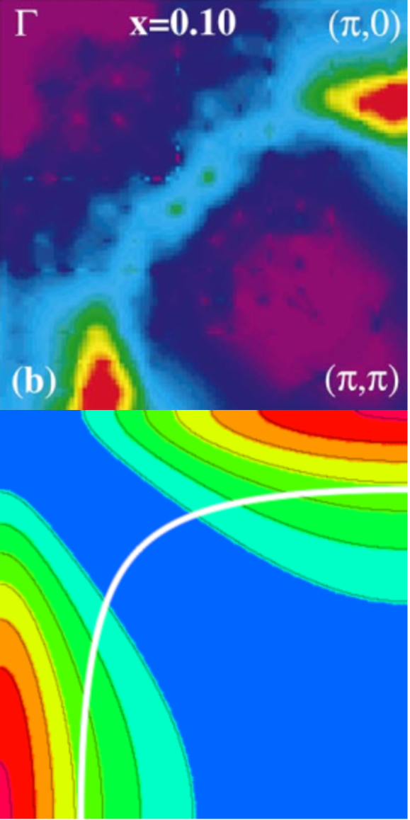
Figure 3: Comparison of the scattering rate calculation in the framework of the s-d exchange calculation (bottom) with the ARPES data from Armitage et al. [54, Fig. 3 (b)] (top); reproduced with permission. The momentum $\mathbf{p}$ dependence of the ARPES intensity for electron energies is close to the Fermi one. Continuous line in the theoretical calculation (bottom) denotes the Fermi contour. The maxima in both figures correspond to hot spots from the phenomenology of Ref. [3]. The coincidence of hot and cold spots is the indispensable qualitative agreement before a detailed theory can be developed.

The comparison depicted in Fig. 3 shows a qualitative similarity, which is encouraging. Originally the hot/cold spot phenomenology was proposed for optimally doped and hole overdoped cuprates. This phenomenology was supported by ARPES studies. However, even for electron doped cuprates, see Fig. 3, the lifetime anisotropy $1/\tau_{\mathbf{p}}$ is qualitatively similar, which is a hint that the microscopic origin is the same.

V Discussion and conclusion

We investigated the electronic properties of a generic CuO₂ plane in the framework of Shubin-Kondo-Zener s-d exchange interaction that simultaneously describes the correlation between T$\!{}_{c}$ and the Cu4s energy. To achieve our goal, we employed the Pokrovsky theory for anisotropic gap BCS superconductors. We used a microscopic model to computed a multiplicatively separable kernel able to simultaneously describe the scattering rate and the superconducting gap anisotropy. Our theoretical approach reproduces the phenomenological analysis of Refs. [3, 4] performed to describe Angle Resolved Photoemission Spectroscopy data.

We conclude that the electric charge fluctuations should be analyzed in the framework of the standard theory of electromagnetic fluctuations in continuous media [41, Chap. 8] and [51, Chap. 6].

The complete theory of ARPES is far beyond our reach, we only wish to point out that hot/cold phenomenology can be derived from a microscopic Hamiltonian describing the superconducting spectrum of the optimally doped and overdoped cuprates. Moreover, it may seem that the named theory is also applicable to underdoped cuprates if additional features like glassy nematicity is included as it has been performed in Ref. [27, Lee, Kivelson and Kim].

Roughly speaking, electrons have only an electric charge and all exchange processes are the result of some projection or Hamiltonian reduction taking into account the Fermi statistics. Every exchange amplitude has to be analyzed in terms of its importance to a variety of viable physical processes. For example, recently the Cu-Cu d-d superexchange was used by Peng et al. for the interpretation of the observation of robust anti-nodal paramagnon modes following spin-wave-like dispersion by resonant inelastic x-ray scattering deep in the normal phase in overdoped cuprates [55]. Moreover, zero sound modes were predicted [56] for layered perovskites with ferromagnetic s-d exchange interaction. Going back to the anti-ferromagnetic s-d exchange interaction, which dominates in many magnetic materials, in the present work we suggest that it can be simultaneously responsible for the gap anisotropy of the superconducting phase and hot/cold spot phenomenology in the normal phase. It would be worthwhile to derive the phenomenological s-d Hamiltonian starting from Hubbard model applied to the CuO₂ plane.

References

- Gozar and Bozovic [2016] A. Gozar and I. Bozovic, High temperature interface superconductivity, Physica C: Supercond. and Appl. 521-522, 38 (2016).
- Mishonov et al. [2022a] T. M. Mishonov, N. I. Zahariev, H. Chamati, and A. M. Varonov, Hot spots along the Fermi contour of high- cuprates explained by - exchange interaction, SN Appl. Sci. 4, 242 (2022a).
- Hlubina and Rice [1995] R. Hlubina and T. M. Rice, Resistivity as a function of temperature for models with hot spots on the Fermi surface, Phys. Rev. B 51, 9253 (1995).
- Ioffe and Millis [1998] L. B. Ioffe and A. J. Millis, Zone-diagonal-dominated transport in high- cuprates, Phys. Rev. B 58, 11631 (1998).
- Pavarini et al. [2001] E. Pavarini, I. Dasgupta, T. Saha-Dasgupta, O. Jepsen, and O. K. Andersen, Band-Structure Trend in Hole-Doped Cuprates and Correlation with , Phys. Rev. Lett. 87, 047003 (2001).
- Röhler [2000] J. Röhler, Plane dimpling and Cu hybridization in YBa2Cu3Ox, Physica B: Cond. Matter 284-288, 1041 (2000).
- Mishonov and Penev [2010] T. M. Mishonov and E. S. Penev, Theory of High Temperature Superconductivity. A Conventional Approach (World Scientific, New Jersey, 2010).
- Andersen et al. [1995] O. Andersen, A. Liechtenstein, O. Jepsen, and F. Paulsen, LDA energy bands, low-energy hamiltonians, , , , and , J. Phys. Chem. Solids 56, 1573 (1995), Procs. Conf. Spectroscopies in Novel Superconductors.
- Andersen et al. [1996] O. K. Andersen, S. Y. Savrasov, O. Jepsen, and A. I. Liechtenstein, Out-of-plane instability and electron-phonon contribution to s- and d-wave pairing in high-temperature superconductors; LDA linear-response calculation for doped CaCuO2 and a generic tight-binding model, J. Low Temp. Phys. 105, 285 (1996).
- Shen and Dessau [1995] Z.-X. Shen and D. Dessau, Electronic structure and photoemission studies of late transition-metal oxides - Mott insulators and high-temperature superconductors, Phys. Rep. 253, 1 (1995).
- Randeria [1996] M. Randeria, High- superconductors: New insights from angle-resolved photoemission, J. Supercond. 9, 471 (1996), arXiv:cond-mat/9709107 [cond-mat.supr-con] .
- Mott [1990] N. F. Mott, Metal-Insulator Transitions, 2nd ed. (Taylor & Francis, London, 1990).
- Abrikosov [1988] A. A. Abrikosov, Fundamentals of the Theory of Metals (North Holland, Amsterdam, 1988).
- Abrikosov [2003] A. Abrikosov, Metal–insulator transition in layered cuprates (SDW model), Physica C: Supercond. 391, 147 (2003).
- Pokrovskii [1961] V. L. Pokrovskii, Thermodynamics of Anisotropic Superconductors, J. Exp. Theor. Phys. 13, 447 (1961), ZhETF 40(2), 641 Aug (1961), http://www.jetp.ras.ru/cgi-bin/r/index/r/40/2/p641?a=list (in Russian).
- Pokrovskii and Ryvkin [1961] V. L. Pokrovskii and M. Ryvkin, Thermodynamics of Anisotropic Superconductors, J. Exp. Theor. Phys. 16, 67 (1961), ZhETF 43(1), 92 Jan (1963), http://www.jetp.ras.ru/cgi-bin/r/index/r/43/1/p92?a=list, (in Russian).
- Mishonov et al. [2021] T. M. Mishonov, N. I. Zahariev, and A. M. Varonov, Hot and cold spots along the Fermi contour of high- cuprates in the framework of Shubin-Kondo-Zener - exchange interaction (2021), arXiv:2111.06716 [cond-mat.supr-con] .
- Landau and Lifshitz [1977] L. D. Landau and E. M. Lifshitz, Quantum Mechanics: Non-Relativistic Theory, 3rd ed., Landau-Lifshitz Course of Theoretical Physics, Vol. 3 (Pergamon, New York, 1977).
- Barišić and Sunko [2022] N. Barišić and D. K. Sunko, High-tc cuprates: a story of two electronic subsystems, J. Supercond. Nov. Magn. 10.1007/s10948-022-06183-y (2022).
- Mishonov et al. [1996] T. M. Mishonov, R. K. Koleva, I. N. Genchev, and E. S. Penev, Quantum chemical calculation of oxygen-oxygen electron hopping amplitude - first principles evaluation of conduction bandwidth in layered cuprates, Czech J. Phys. 46, 2645 (1996).
- Vishik et al. [2010] I. M. Vishik, W. S. Lee, R.-H. He, M. Hashimoto, Z. Hussain, T. P. Devereaux, and Z.-X. Shen, ARPES studies of cuprate Fermiology: superconductivity, pseudogap and quasiparticle dynamics, New J. Phys. 12, 105008 (2010).
- Kaminski et al. [2005] A. Kaminski, H. M. Fretwell, M. R. Norman, M. Randeria, S. Rosenkranz, U. Chatterjee, J. C. Campuzano, J. Mesot, T. Sato, T. Takahashi, T. Terashima, M. Takano, K. Kadowaki, Z. Z. Li, and H. Raffy, Momentum anisotropy of the scattering rate in cuprate superconductors, Phys. Rev. B 71, 014517 (2005), arXiv:cond-mat/0404385 [cond-mat.str-el] .
- Zonno et al. [2021] M. Zonno, F. Boschini, and A. Damascelli, Time-resolved ARPES on cuprates: Tracking the low-energy electrodynamics in the time domain, J. Electron Spectrosc. 251, 147091 (2021), arXiv:2106.11316 [cond-mat.supr-con] .
- Dimitrov et al. [2011] Z. Dimitrov, S. Varbev, K. Omar, A. Stefanov, E. Penev, and T. Mishonov, Correlation between and the Cu Level Reveals the Mechanism of High-Temperature Superconductivity, Bulg. J. Phys. 38, 106 (2011).
- Damascelli et al. [2003] A. Damascelli, Z. Hussain, and Z.-X. Shen, Angle-resolved photoemission studies of the cuprate superconductors, Rev. Mod. Phys. 75, 473 (2003).
- Lee et al. [2006] P. A. Lee, N. Nagaosa, and X.-G. Wen, Doping a Mott insulator: Physics of high-temperature superconductivity, Rev. Mod. Phys. 78, 17 (2006), arXiv:cond-mat/0410445 [cond-mat.str-el] .
- Lee et al. [2016] K. Lee, S. A. Kivelson, and E.-A. Kim, Cold-spots and glassy nematicity in underdoped cuprates, Phys. Rev. B 94, 014204 (2016).
- Mishonov and Groshev [1994] T. Mishonov and A. Groshev, Two-electron exchange between adjacent oxygen atoms as a possible origin of the pairing in layered cuprates, Physica B 194–196, 1427 (1994).
- Mishonov et al. [1998] T. M. Mishonov, A. V. Groshev, and A. A. Donkov, Pairing in layered cuprates by two-electron exchange between adjacent oxygen ions, Bulg. J. Phys. 25, 62 (1998).
- Mishonov et al. [2002] T. M. Mishonov, J. P. Wallington, E. S. Penev, and J. O. Indekeu, Reduced pairing hamiltonian for interatomic two-electron exchange in layered cuprates, Mod. Phys. Lett. B 16, 693 (2002), cond-mat/0205616 .
- White and Geballe [1979] R. M. White and T. H. Geballe, Long–Range Order in Solids, Solid State Physics (Academic Press, New York, 1979).
- White [2007] R. M. White, Quantum Theory of Magnetism, 3rd ed., Springer Series in Solid-State Sciences (Springer, Berlin, 2007).
- Anders [2012] F. Anders, The Kondo Effect, in Correlated electrons: from models to materials, Vol. 2, edited by E. Pavarini (Forschungszentrum Jülich GmbH Zenralbibliothek, Verlag, Jülich, 2012) Chap. 11.
- Eickhoff et al. [2018] F. Eickhoff, B. Lechtenberg, and F. B. Anders, Effective low-energy description of the two-impurity Anderson model: RKKY interaction and quantum criticality, Phys. Rev. B 98, 115103 (2018).
- Eickhoff and Anders [2020] F. Eickhoff and F. B. Anders, Strongly correlated multi-impurity models: The crossover from a single-impurity problem to lattice models, Phys. Rev. B 102, 205132 (2020).
- Eickhoff and Anders [2021a] F. Eickhoff and F. B. Anders, Kondo holes in strongly correlated impurity arrays: RKKY-driven Kondo screening and hole-hole interactions, Phys. Rev. B 104, 045115 (2021a).
- Eickhoff and Anders [2021b] F. Eickhoff and F. B. Anders, Spectral properties of strongly correlated multi-impurity models in the Kondo insulator regime: Emergent coherence, metallic surface states, and quantum phase transitions, Phys. Rev. B 104, 165105 (2021b).
- Einstein [1905] A. Einstein, Über die von der molekularkinetischen Theorie der Wärme geforderte Bewegung von in ruhenden Flüssigkeiten suspendierten Teilchen, Annalen der Physik 322, 549 (1905).
- Rayleigh [1899] L. Rayleigh, XXXIV. On the transmission of light through an atmosphere containing small particles in suspension, and on the origin of the blue of the sky, Phil. Mag. 47, 375 (1899).
- Mishonov and Mishonov [2000] T. M. Mishonov and M. T. Mishonov, Simple model for the linear temperature dependence of the electrical resistivity of layered cuprates, Physica A 278, 553 (2000).
- Lifshitz and Pitaevskii [1980a] E. M. Lifshitz and L. P. Pitaevskii, Statistical Physics. Part 2, Landau-Lifshitz course of theoretical physics, Vol. 9 (Pergamon, New York, 1980).
- Mishonov and Groshev [1990] T. M. Mishonov and A. Groshev, Plasmon excitations in josephson arrays and thin superconducting layers, Physical Review Letters 64, 2199 (1990).
- Buisson et al. [1994] O. Buisson, P. Xavier, and J. Richard, Observation of Propagating Plasma Modes in a Thin Superconducting Film, Phys. Rev. Lett. 73, 3153 (1994).
- Logvenov et al. [2009] G. Logvenov, A. Gozar, and I. Bozovic, High-Temperature Superconductivity in a Single Copper-Oxygen Plane, Sci 326, 699 (2009).
- Baber [1937] W. G. Baber, The contribution to the electrical resistance of metals from collisions between electrons, Proc. R. Soc. London, Ser. A 158, 383 (1937).
- Landau and Pomeranchuk [1936] L. Landau and I. Pomeranchuk, Über die Eigenschaften der Metalle bei sehr niedrigen Temperaturen, Phys. Z. Sowjetunion 10, 649 (1936), (in German).
- Lifshitz and Pitaevskii [1980b] E. M. Lifshitz and L. P. Pitaevskii, Physical Kinetics, Landau-Lifshitz course of theoretical physics, Vol. 10 (Pergamon, New York, 1980).
- Herapath [1821] J. Herapath, A Mathematical Inquiry into the Causes, Laws, and principal Phenomena of Heat, Gases, Gravitation, Ann. Phil. New Series 1, 273 (1821).
- Waterston and Beaufort [1851] J. J. Waterston and F. Beaufort, On the Physics of media that are composed of free and perfectly elastic molecules in a state of motion, Proc. R. Soc. Lond. 5, 604 (1851).
- Waterston et al. [1892] J. J. Waterston, F. Beaufort, and J. W. Strutt, I. n the physics of media that are composed of free and perfectly elastic molecules in a state of motion, Phil. Trans. R. Soc. Lond. A 183, 1 (1892).
- Abrikosov et al. [1963] A. A. Abrikosov, L. P. Gor’kov, and I. Y. Dzyaloshinskii, Methods of quantum field theory in statistical physics (Prentice Hall, Englewood Cliffs, N.J., 1963).
- Rosch [2000] A. Rosch, Magnetotransport in nearly antiferromagnetic metals, Phys. Rev. B 62, 4945 (2000).
- Lee [2021] P. A. Lee, Low-temperature T-linear resistivity due to umklapp scattering from a critical mode, Phys. Rev. B 104, 035140 (2021), arXiv:2012.09339 [cond-mat.str-el] .
- Armitage et al. [2002] N. P. Armitage, F. Ronning, D. H. Lu, C. Kim, A. Damascelli, K. M. Shen, D. L. Feng, H. Eisaki, Z.-X. Shen, P. K. Mang, N. Kaneko, M. Greven, Y. Onose, Y. Taguchi, and Y. Tokura, Doping Dependence of an -Type Cuprate Superconductor Investigated by Angle-Resolved Photoemission Spectroscopy, Phys. Rev. Lett. 88, 257001 (2002), arXiv:cond-mat/0201119 [cond-mat.str-el] .
- Peng et al. [2018] Y. Y. Peng, E. W. Huang, R. Fumagalli, M. Minola, Y. Wang, X. Sun, Y. Ding, K. Kummer, X. J. Zhou, N. B. Brookes, B. Moritz, L. Braicovich, T. P. Devereaux, and G. Ghiringhelli, Dispersion, damping, and intensity of spin excitations in the monolayer cuprate superconductor family, Phys. Rev. B 98, 144507 (2018).
- Mishonov et al. [2022b] T. M. Mishonov, N. I. Zahariev, H. Chamati, and A. M. Varonov, Possible zero sound in layered perovskites with ferromagnetic - exchange interaction, SN Appl. Sci. 4, 228 (2022b).