Is there a tensionless Kardar-Parisi-Zhang universality class above one dimension?
An Ising model approach

Abstract

The Kardar-Parisi-Zhang (KPZ) equation is a paradigm of generic scale invariance, for which it represents a conspicuous universality class. Recently, the tensionless case of this equation has been shown to provide a different universality class by itself. This class describes the — intrinsically anomalous — scaling of one-dimensional (1D) fronts for several physical systems that feature ballistic dynamics. In this work, we show that the evolution of certain 1D fronts defined for a 2D Ising system also belongs to the tensionless KPZ universality class. Nevertheless, the Ising fronts exhibit multiscaling, at variance with the continuous equation. The discrete nature of these fronts provides an alternative approach to assess the dynamics for the 2D front case (for a 3D Ising system), since the direct integration of the tensionless KPZ equation blows up in this case. In spite of the agreement between the 1D scaling of the Ising fronts and the tensionless KPZ equation, the fluctuation statistics in 1D and the full behavior in 2D are strongly conditioned by boundary effects.

I Introduction

The Kardar-Parisi-Zhang (KPZ) equation Kardar86 is a paradigm for nonequilibrium systems in which generic scale invariance (GSI) occurs Grinstein95 ; Tauber14 . It is the representative of an universality class for space-time criticality — characterized by how the amplitude of the field fluctuations scales in space and time and how these fluctuations are statistically distributed Barabasi95 ; Krug97 ; Kriechebauer10 ; Corwin12 ; Halpin-Healy15 ; Takeuchi18 — in absence of parameter tuning, which describes a wide variety of systems with strong correlations. Some of these systems include turbulent liquid crystals Takeuchi11 , stochastic hydrodynamics Mendl13 , colloidal aggregation Yunker13 , reaction-diffusion systems Nesic14 , random geometry Santalla15 ; Santalla17 , active matter Chen16 , thin films Orrillo17 , superfluidity Altman15 , quantum entanglement Nahum17 , electronic fluids Protopopov21 , and both integrable and non-integrable quantum spin chains Gopalakrishnan19 ; Ljubotina19 ; DeNardis21 . Specifically, the KPZ equation describes the evolution of a scalar field $h(\vec{x},t)$ representing e.g. the height of an interface above point $\vec{x}$ on a substrate in $\mathbb{R}^{d}$ at time $t$, as Kardar86

$$\partial_{t}h=\nu\nabla^{2} h+\frac{\lambda}{2}(\nabla h)^{2}+\eta(\vec{x},t),$$ (1)

$$\langle\eta(\vec{x},t)\eta(\vec{x}^{\prime},t^{\prime})\rangle =2D\,\delta(\vec{x}-\vec{x}^{\prime})\delta(t-t^{\prime}),$$

where $\nu,D>0$, and $\lambda$ are parameters, and $\eta(\vec{x},t)$ is zero-average, Gaussian white noise.

While the nonlinear term in Eq. (1) approximates growth of the front or interface profile $h$ along the local normal direction and the noise term introduces the stochasticity of microscopic growth events in space and time, the diffusive linear term induces a local smoothening mechanism in which $\nu$ plays the role of a surface tension parameter Barabasi95 ; Krug97 . In absence of this smoothening mechanism, Eq. (1) becomes the so-called tensionless KPZ equation, namely,

$$\partial_{t}h=\frac{\lambda}{2}(\nabla h)^{2}+\eta.$$ (2)

For one-dimensional (1D) substrates where $d=1$, solutions to Eq. (2) can not be derived from the exact results available for the full KPZ equation Kardar86 ; Kriechebauer10 ; Corwin12 ; Halpin-Healy15 , which require the Cole-Hopf transformation $H(x,t)=\exp[\lambda h(x,t)/(2\nu)]$. In higher dimensions, there are not exact analytical solutions even for the $\nu\neq 0$ KPZ equation. Hence, numerical approaches are necessary to assess the behavior of Eq. (2). Alternatively, discrete models in the same universality class could provide a description of the solutions of this equation.

Equation (2) has been proved to be marginally unstable to perturbations of a flat solution Golubovic91 ; Cuerno95 . Hence, the numerical integration is ardous and well-posedness of the equation has been questioned Tabei04 ; Bahraminasab04 . However, successful integration has been recently achieved for 1D substrates Rodriguez-Fernandez22b ; Cartes22 . Specifically, in Ref. Rodriguez-Fernandez22b the scaling exponents and fluctuation statistics have been determined for Eq. (2) in 1D, leading to the identification of a new universality class Rodriguez-Fernandez22b , determined by intrinsic anomalous kinetic roughening Schroeder93 ; DasSarma94 ; Lopez97 ; Ramasco00 and exponent values $\alpha=\beta=z=1$, and $\alpha_{s}=1/2$, see Sec. II below for their precise definitions. This scaling may be compatible with that found in experimental physical systems like quantum spin chains Wei21 , in which different parameter conditions exhibit scaling which seems consistent with either the $\nu=0$ or $\nu\neq 0$ KPZ equations. The scaling behavior elucidated for Eq. (2) also seems consistent to a varying degree of detail with the kinetic roughening behavior obtained for growth models related with isotropic percolation Asikainen02 ; Asikainen02b , colloidal aggregates Yunker13 , and in the equilibrium state of certain magnetic systems Dashti-Naserabadi19 . However, very little is known regarding this universality class of Eq. (2) in higher dimensions, including the $d=2$ case, where numerical simulations of Eq. (2) present stability issues Rodriguez-Fernandez22 . This coincides with expectations from some previous results reported in the literature Bahraminasab04 , in which a surface described by the 2D KPZ equation is argued to become multivalued in the $\nu\to 0$ limit.

In this work, we assess an alternative approach to the tensionless KPZ universality class along a route that avoids direct numerical integration of Eq. (2). Specifically, we formulate and study a discrete model, in principle free from the numerical instabilities that may arise due to discrete approximations of continuous equations, and which may potentially belong to the same universality class of Eq. (2). To this end, we consider the scaling behavior of the 1D interface associated with an equilibrium 2D Ising model at its critical temperature $T=T_{c}$, that has been studied in Ref. Dashti-Naserabadi19 . While the relation between the Ising model and the KPZ equation had been studied much earlier for the $\nu\neq 0$ case Grossmann91 , the precise model put forward in Ref. Dashti-Naserabadi19 seems to suit our present $\nu=0$ condition. Specifically, the authors of that work observe the same static type of intrinsically anomalous scaling and the same exponent values as those found to describe the spatial behavior of the fluctuations in the tensionless KPZ equation Rodriguez-Fernandez22b . However, no time-related exponents are measured in Ref. Dashti-Naserabadi19 . In our present paper, we study the full dynamics of this process in order to determine if the scaling behavior corresponds to that in the tensionless KPZ equation not only in space, but also in time. We perform simulations of the evolution of Ising spin domains in 2D and 3D, using both a Metropolis algorithm and an alternative coarse-grained approach based on the Ginzburg-Landau equation, using the boundary conditions proposed in Ref. Dashti-Naserabadi19 and described in Fig. 1.

This paper is organized as follows. In section II, we describe the observables that we will measure in the characterization of the scaling of kinetic roughening processes. In section III, we describe the boundary conditions of the Ising model we will deal with, the definition of the front, and the two different approaches followed for the simulation of the evolution of the system. Then, we describe the numerical results obtained both for 1D and 2D fronts (related with 2D and 3D Ising systems, respectively) via our Ginzburg-Landau approach in sections IV and V. The results we have obtained via a Metropolis Monte Carlo approach are presented in an Appendix. We provide a discussion of our results in section VI, which is followed by a summary and our conclusions in section VII.

II Observables

The observables which are going to be used in the characterization of the front dynamics are (i) the global roughness,

$$W(t)=\Big{\langle}\sqrt{{\frac{1}{L^{d}}}\int_{[0,L]^{d}}[h(\vec{x},t)-\bar{h}(t)]^{2}d\vec{x}}\Big{\rangle},$$ (3)

where bar denotes spatial average, $L$ is the lateral system size, and brackets denote average over different realizations of the noise, (ii) the structure factor

$$S(\vec{k},t)=\langle|\hat{h}(\vec{k},t)|^{2}\rangle,$$ (4)

where $\hat{h}(\vec{k},t)$ is the Fourier transform of $h(\vec{x},t)$ and $\vec{k}$ is $d$-dimensional wave vector, and (iii) the height-difference correlation function,

$$G_{2}(\vec{r},t)=\sqrt{\langle[\overline{h(\vec{x}+\vec{r},t)-h(\vec{x},t)}]^{2}\rangle}.$$ (5)

In a kinetic roughening process Barabasi95 , the global roughness scales as $W\sim t^{\beta}$ — with $\beta$ being the so-called growth exponent — up to a saturation value $W_{sat}\sim L^{\alpha}$ which is reached at steady state — here, $\alpha$ is the so-called roughness exponent, which is related to the fractal dimension $D_{f}$ of the front considered as a self-affine fractal, as $\alpha=d+1-D_{f}$ Barabasi95 . The time $t_{sat}$ required for the system to reach the steady state scales as $t_{sat}\sim t^{z}$. Here, $z=\alpha/\beta$ is the so-called dynamic exponent, which characterizes the time dependence of the lateral correlation length $\xi$ along the front as $\xi\sim t^{1/z}$ Barabasi95 . It is possible to define a scaling function $f_{W}$ that summarizes these scaling laws into the single expression

$$W(L,t)\sim L^{\alpha}f_{W}\left(\frac{t}{L^{z}}\right),$$ (6)

namely,

$$f_{W}(u)\sim\left\{\begin{array}[]{lcc}u^{\beta}&\mathrm{if}&u\ll 1,\\ \mathrm{Constant}&\mathrm{if}&u\gg 1\end{array}\right.,$$ (7)

The local roughness measured over windows of size $l<L$ also scales with the window size $l$, with a local exponent $\alpha_{loc}$. Equivalently, the height-difference correlation function, Eq. (6), scales as $G_{2}\sim|\vec{r}|^{\alpha_{loc}}$. In general, $\alpha_{loc}=\alpha$ (e.g. in the KPZ equation for $\nu\neq 0$ Barabasi95 ). However, there are some kinetic roughening systems (e.g., the tensionless KPZ equation Rodriguez-Fernandez22b ) in which the local and the global scalings of the roughness with the window size are different, i.e. $\alpha_{loc}\neq\alpha$. Such a behavior is called anomalous scaling or anomalous kinetic roughening Schroeder93 ; DasSarma94 ; Lopez97 . The structure factor scales in this case as Ramasco00

$$S(\vec{k},t)\sim|\vec{k}|^{-(2\alpha+d)}f_{S}(|\vec{k}|^{z}t),$$ (8)

where $f_{S}$ behaves as

$$f_{S}(u)\sim\left\{\begin{array}[]{lcc}u^{2\alpha+d}&{\rm if}&u\ll 1\\ u^{2(\alpha-\alpha_{s})}&{\rm if}&u\gg 1.\end{array}\right.$$ (9)

Here, $\alpha_{s}$ is an exponent measured in Fourier space which is equal to $\alpha_{loc}$ when $\alpha_{loc}<1$ Ramasco00 . For $\alpha=\alpha_{loc}$, the scaling behavior described by Eq. (9) is the standard Family-Vicsek Barabasi95 . Anomalous scaling has been conjectured, via perturbative arguments, not to be in the asymptotic regime of continuum models which feature local interactions and time-dependent noise Lopez05 .

Additionally, we will also check multiscaling behavior, where higher moments of the height-difference correlation function, namely

$$G_{q}(\vec{r},t)=\langle|h(\vec{x}+\vec{r},t)-h(\vec{x},t)|^{q}\rangle^{1/q}$$ (10)

do not scale with the same roughness exponent for different values of $q$, i.e. for which $G_{q}(r)\sim r^{\alpha_{q}}$ with a $q$-dependent $\alpha_{q}$. In those cases, the morphologies are said to be multi-affine Barabasi95 . This kind of surfaces appear in e.g. surface growth models related with isotropic percolation Asikainen02 ; Asikainen02b .

III System description

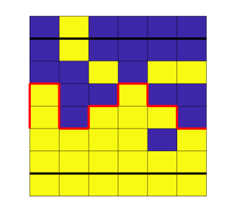
Figure 1: Definition of the height profile $h(x)$ (red solid line) from a certain $6\times 6$ spin domain (yellow and blue colors correspond to $+1$ and $-1$ spin values, respectively). The spin rows below and above the bottom and top black solid lines illustrate the Dirichlet and Neumann boundary conditions, respectively, see the main text. All units are arbitrary.

The physical system that we study in this work is in principle the same as that proposed in Ref. Dashti-Naserabadi19 . We define a 1D (2D) interface or front $h(x,(y))$ from a 2D (3D) spin domain $\{s_{i,(j),k}\}$, where $s_{i,(j),k}=\pm 1$ are Ising spins, $i,j,k=1,2,...,L$. Dirichlet (fixed) and Neumann (free) boundary conditions are fixed on each boundary in one of the system dimensions (the “vertical” or “growth” one); specifically, $s_{i,(j),0}=+1$ and $s_{i,(j),L+1}=s_{i,(j),L}$, respectively. Periodic boundary conditions are considered in the other (transverse or substrate) dimensions, i.e., $s_{0,(j),k}=s_{L,(j),k}$, $s_{L+1,(j),k}=s_{1,(j),k}$, $s_{i,(0),k}=s_{i,(L),k}$, and $s_{i,(L+1),k}=s_{i,(1),k}$. We will refer to this set of boundary conditions as magnet. Then, a set $\mathcal{C}_{i,(j),k}$ is defined, such that $\mathcal{C}_{i,(j),k}=1$ for all the spins aligned with the $+1$ spins fixed at the Dirichlet bottom boundary, which are connected to each other via nearest-neighbor paths, and $\mathcal{C}_{i,(j),k}=0$ otherwise. The height of the interface at a certain time $t$ is finally defined as

$$h(x,(y))=\sum_{k=1}^{L}\mathcal{C}_{i,(j),k}.$$ (11)

An illustrative 2D spin domain with $L=6$ under these boundary conditions, as well as its corresponding $h(x)$ interface profile, is depicted in Fig. 1.

III.1 Metropolis approach

The most straightforward way for the study of the dynamical evolution of the spin configurations of a ferromagnetic system consists in the use of Monte Carlo simulations Newman99 . A Metropolis algorithm can be used in order to simulate the full evolution of the spin field, while the equilibrium state of the model described in the previous paragraph was studied in Ref. Dashti-Naserabadi19 using Wolff’s algorithm. For each Monte Carlo step, one random spin in a position $\vec{r}=i,j,(k)$ is chosen and flipped with probability $P_{\vec{r}}$, such that

$$P_{\vec{r}}=\left\{\begin{array}[]{lcc}e^{-\Delta E_{\vec{r}}/k_{B}T}&{\rm if}&\Delta E_{i,j,(k)}>0,\\ \\ 1/2&{\rm if}&\Delta E_{i,j,(k)}=0,\\ \\ 1&{\rm if}&\Delta E_{i,j,(k)}<0,\end{array}\right.$$ (12)

where

$$H[\{s_{\vec{r}}\}]=-J\sum_{\vec{r}}s_{\vec{r}}\big{(}\sum_{\vec{r}^{\prime}\in\mathcal{N}(\vec{r})}\ s_{\vec{r}^{\prime}}\big{)}$$ (13)

is the Ising Hamiltonian, $\mathcal{N}(\vec{r})$ is the set of all the nearest-neighbours for the position $\vec{r}$ on the square lattice, $J>0$ is a ferromagnetic coupling, and $k_{B}$ is Boltzmann’s constant. Hence, $\Delta E_{\vec{r}}=2Js_{\vec{r}}\left(\sum_{\vec{r}^{\prime}\in\mathcal{N}(\vec{r})}\ s_{\vec{r}^{\prime}}\right)$ is the energy change due to the spin flip at position $\vec{r}$. The time scale is set to $t=N/L^{d}$, where $N$ is the number of Monte Carlo steps.

This method yields a behavior in which boundary effects strongly affect the evolution of the front $h(x,(y),t)$, so that its scaling can not be unambiguously assessed for the system sizes we have been able to simulate. The details about these results are described in Appendix A. In view of this fact, we alternatively employ a coarse-grained approach that allows us to access the effective behavior of larger systems via the time-dependent Ginzburg-Landau equation.

III.2 Ginzburg-Landau approach

The Ginzburg-Landau (GL) equation Garcia-Ojalvo_Book

$$\partial_{t}m=\frac{1}{2}\left(\nabla^{2}m+m-m^{3}\right)+\tilde{D}\eta,$$ (14)

where $m(\vec{x},t)$ denotes the local magnetization field and $\eta$ is an uncorrelated white noise term, is an effective coarse-grained model, well-known to describe the evolution of the scalar magnetization of an Ising ferromagnet around thermal equilibrium Garcia-Ojalvo_Book ; Taverniers14 . We use this model in order to simulate the full dynamic evolution of our Ising system. We also define here a coarse-grained spin lattice $\{s_{\vec{r}}\}$ by discretizing $s_{\vec{r}}=+1$ if $m(\vec{r})>0$ and $s_{\vec{r}}=-1$ otherwise, from which we will define the field $h(x,(y))$ using Eq. (11). The same boundary conditions as those proposed in Ref. Dashti-Naserabadi19 are considered, see Fig. 1.

Our purpose is to assess the behavior of this coarse-grained spin system at the noise amplitude value $\tilde{D}=\tilde{D_{c}}$ corresponding to the Ising critical temperature $T_{c}$. For such a value of the noise, the relative fluctuation of the local magnetization field,

$$M=\frac{\langle m^{2}(\vec{x})\rangle-\langle m(\vec{x})\rangle^{2}}{L^{d}{\tilde{D}}},$$ (15)

exhibits a divergence at steady state as $M\sim L^{\gamma/\nu}$. Here, $\gamma=7/4$ and $\nu=1$ are the exact Ising critical exponents in two dimensions Garcia-Ojalvo_Book and $\gamma\simeq 1.23$ and $\nu\simeq 0.63$ are the approximate values in three dimensions Cardy_book .

Numerical simulations of Eq. (14) have been carried out in real space. A straightforward finite-difference scheme in space and an Euler scheme in time have been employed Garcia-Ojalvo_Book , using $\Delta t=0.1$ and $\Delta x=1$. A homogeneous initial condition $m(i,(j),k)=-1$ for all $i,j,k=1,2,...,L$ has been considered, while the opposite spin value has been considered at the Dirichlet boundary corresponding to $i=0$.

IV Dynamics at $T=T_{c}$ for a one-dimensional interface

IV.1 Scaling exponents and front fluctuations

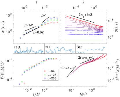
Figure 2: Time evolution for the roughness $W(t,L)$ and the structure factor $S(k,t)$ of the field $h(x,t)$ defined from the simulations of Eq. (14) for a 2D domain. Time values increase bottom to top in $S(k,t)$ and coincide with those shown for $W(t)$. The data collapses for the roughness $W(t,L)$ and structure factor $S(k,t)$ are also shown. Morphologies $h(x)$ for random deposition (R.D.), nonlinear growth (N.L.), and saturation (Sat.) regimes are depicted. All units are arbitrary.

The full critical dynamics of the field $h(x,t)$ is evaluated at $\tilde{D}=\tilde{D}_{c}$. In Ref. Rodriguez-Fernandez22 it is shown that $\tilde{D}_{c}\simeq 0.9$ corresponds to the critical temperature $T=T_{c}$ of the 2D Ising model not only with periodic boundary conditions Garcia-Ojalvo_Book but also with the magnet boundary conditions shown in Fig. 1.

In Fig. 2, the evolution of both the surface roughness $W(t)$ and the structure factor $S(k,t)$ are depicted, together with the data collapses corresponding to the scaling exponents of the tensionless KPZ equation Rodriguez-Fernandez22b , namely $\alpha=1$, $\alpha_{s}=1/2$, and $z=1$, hence $\beta=1$, which are accurate for large times prior to saturation to steady state. A random deposition-like Barabasi95 regime [with $\beta\simeq 0.62>1/2$ and $k$-independent $S(k)$] is observed at short times, as for the tensionless KPZ equation Rodriguez-Fernandez22b . In this case, the effective growth exponent is slightly larger than the exact random deposition value $1/2$. Morphologies for $h(x,t)$ profiles, for times in the random deposition, nonlinear growth, and steady state regimes are also depicted.

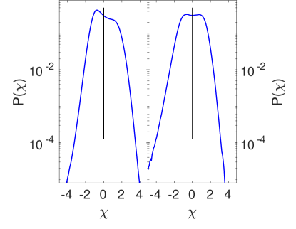
Figure 3: Probability density function for the height fluctuations $\chi=(h-\bar{h})/{\rm std}(h)$ over 5000 realizations from simulations of the GL model in 2D at critical noise $\tilde{D}=0.9\simeq\tilde{D}_{c}$ and $L=128$, for $t=200$ (left panel) and $t=1600$ (right panel). All units are arbitrary.

In order to assess the full equivalence between this model and the tensionless KPZ equation in terms of universality classes of kinetic roughening, i.e. scaling exponents and fluctuations statistics, the fluctuations of the height field $h(x,t)$ should be measured at different times. For the tensionless KPZ equation, the probability density function (PDF) is non-symmetric during the growth regime, while at steady state it becomes symmetric, very flat in its central part and with Gaussian tails Rodriguez-Fernandez22b . Numerical results on the PDF of the height fluctuations for our 1D fronts are shown in Fig. 3. The fluctuations distribution is distorted by the Dirichlet and Neumann boundary conditions at the bottom and the top of the domain, respectively. At relatively short times before saturation to steady state, when some parts of the height profile are still close to the bottom (Dirichlet) boundary, the negative range of the fluctuations become over-represented, see the left panel of Fig. 3. At longer times, the approach to the upper (Neumann) boundary appears to induce a second over-representation, now for a positive range of fluctuations. To avoid this effect as much as possible in the construction of the fluctuation histograms, we have discarded morphologies in which the upper part of the $h(x,t)$ field touches the upper boundary of the domain. This makes us reject noise realizations very easily, requiring a large number of runs to assess the system behavior at moderate and long times. At steady state, the resulting fluctuations are both symmetric and relatively flat close to the origin (see right panel of Fig. 3), but both medium-low and medium-large values are over-represented. Hence, in spite of these rejections, the boundary effects may still be playing an important role in the shape of the fluctuation PDF for the system size studied. We expect much larger system sizes to enable avoidance of these boundary effects and to allow for an unbiased assessment of the actual fluctuation PDF; however, this would be very intensive in computational resources, both in terms of memory and processing.

In order to further illustrate the interplay of the morphology with the boundary conditions, we show in Fig. 4 the time evolution of the mean value of $h$, as well as some morphologies $h(x,t)$ at different times, both in the growth regime and at saturation to steady state. We identify only a narrow interval of $t$ (from $t_{2}$ to $t_{3}$, approximately) for which $\overline{h}\pm{\rm std}(h)$ is close to no system boundary. However, as seen in the depicted morphologies $h(x,t_{2})$ and $h(x,t_{3})$, there are still individual realizations for which some parts of the surface $h(x,t)$ are close to the top and/or bottom boundaries, thus influencing the shape of the fluctuation PDF.

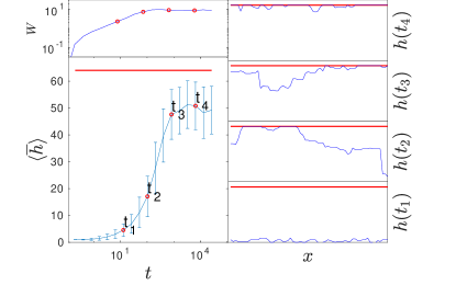
Figure 4: Time evolution of the average mean height profile $\langle\bar{h}\rangle$, as obtained over 100 noise realizations, from numerical simulations of the GL model (left bottom panel), compared to the maximum achievable height (domain lateral size, horizontal red solid line). Error bars correspond to the roughness of the front for each time. Left top panel shows the corresponding evolution of the height roughness $W(t)$. One realization of the $h(x,t)$ morphology for each one of the highlighted times, $t_{1}$ to $t_{4}$, in the left panels is shown in the right panels. All units are arbitrary.

IV.2 Multiscaling

In spite of having the same scaling exponents values and intrinsically anomalous roughening behavior, morphologies in the nonlinear growth regime from the tensionless KPZ equation (see Ref. Rodriguez-Fernandez22b ) and from the GL model in 2D (see Fig. 2) exhibit quite different shapes to the naked eye, due in particular to the abundance of prominent slopes in the latter, while in the former the slope distribution is Gaussian Rodriguez-Fernandez22b . We assess the PDF of the slope field $u=\partial_{x}h$ for the GL interfaces in Fig. 5.

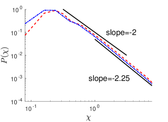
Figure 5: Histogram of slope values [$\chi=(u-\bar{u})/{\rm std}(u)$, where $u=\partial_{x}h$] from morphologies of the 2D GL growth model within the nonlinear regime identified in Fig. 2. Dashed red and dashed-dotted blue lines correspond to $L=128$ and $L=256$, respectively. All units are arbitrary.

We observe in the figure that the tail of the PDF decays approximately as a power law ${P}(\chi)\sim\chi^{-2}$. In Ref. Asikainen02 ; Asikainen02b , this type of slope statistics has been shown to imply multiscaling behavior, as different $q$-moments of the height-difference distribution, Eq. (10), were then shown not to scale with the same roughness exponent $\alpha$ for different values of $q$. Specifically, in Refs. Asikainen02 ; Asikainen02b a surface growth model related with isotropic percolation (invasion percolation without trapping) was studied numerically, finding that the statistics was well described by the power law ${P}(\chi)\sim\chi^{-2}$. In that case, a scaling analysis based on isotropic percolation implies that $\alpha_{q}=1/q$ for arbitrary $q$. This seems to be also the case in our present numerical simulations, quite accurately for $q>1$, as shown in Fig. 6. Such a multi-fractal property of the morphologies defined in our GL model is a remarkable qualitative difference between them and the morphologies described by the tensionless KPZ equation, in which the fast decay of the fluctuations in $h$ induced by Gaussian-distributed slopes $u=\partial_{x}h$ prevents multi-fractality from taking place Asikainen02 ; Asikainen02b .

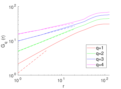
Figure 6: First, second, third, and fourth moments (bottom to top) of the height-difference correlation function $G_{q}(r)$ from numerical simulations of the 2D GL model in the nonlinear growth regime identified in Fig. 2. Dashed straight lines correspond to the exact values of the slopes $\alpha_{q}=1/q$, as predicted in Refs. Asikainen02 ; Asikainen02b . All units are arbitrary.

V Dynamics at $T=T_{c}$ for a two-dimensional interface

The study of the behavior of the tensionless KPZ equation for 2D substrates was not possible by numerically integrating the tensionless KPZ, Eq. (2), directly due to finite-time blow-up phenomena Rodriguez-Fernandez22 . We consider here an alternative approach by studying the dynamics of the spin configurations in three spatial dimensions which lead to the time evolution of two-dimensional interfaces $h(x,y,t)$. The noise amplitude that corresponds to the critical temperature in a 3D system is assessed again in analogy to our work for 2D spin domains. In this case, the critical $\tilde{D}$ takes the value $\tilde{D}_{c}\simeq 1.25$ Rodriguez-Fernandez22 .

In principle, we can now assess the behavior of the corresponding $h(x,y,t)$ profiles in terms of their kinetic roughening universality class. The evolution of the front roughness $W(t)$ is depicted for different system sizes in Fig. 7. The growth of the roughness is suddenly interrupted and $W$ starts to decay for $t\gtrsim 20$. This behavior is induced by the upper boundary as we can appreciate in Fig. 8. The mean height $\overline{h}$ suddenly approaches the upper boundary at the same time in which the growth of the roughness is interrupted. For longer times the surface becomes pinned to this boundary, leading to the decrease in the roughness from that time on, much as it happens in our Metropolis approach both for 1D and 2D fronts (see Appendix A). Both under the GL approach and under the Monte Carlo approach assessed in the Appendix, the peak value for $W(t)$ reached in the 2D interfaces increases with the system size. Hence, it may diverge to infinity for an infinite system, being a discrete analogue of finite time blow-up in a continuous system.

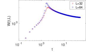
Figure 7: Time evolution of the roughness $W$ for the height profiles obtained from numerical simulations of the GL model in three-dimensional domains, using boundary conditions as described in Fig. 1, and for different values of the lateral system size $L$.

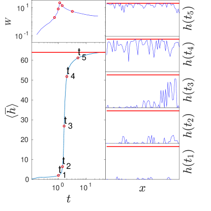
Figure 8: Time evolution of the average mean height profile $\langle\bar{h}\rangle$ obtained over 10 realizations of the noise from numerical simulations of the 3D GL model (left bottom panel) compared to the maximum achievable height (domain lateral size, horizontal red solid line). Left top panel shows the corresponding evolution of the surface roughness $W(t)$. One realization of a longitudinal cut $h(x,1,t)$ for each one of the highlighted times, $t_{1}$ to $t_{4}$ in the left panels, is shown in the right panels. All units are arbitrary.

VI Discussion

We have assessed the tensionless KPZ universality class Rodriguez-Fernandez22b in an alternative way with respect to the explicit tensionless KPZ equation itself, namely, via a discrete growth model defined for an Ising spin system. In principle, this approach allows us to circumvent the finite-time blow-up occurring in the numerical integration of the 2D tensionless KPZ equation, and it may eventually do so for even higher dimensions. This 2D case could have a potential interest in the context of surface growth, where many experimental systems are over 2D substrates, as for e.g. thin film deposition Seshan18 .

For one-dimensional fronts, we have found that the full dynamics of the discrete model defined in an Ising system based on the equilibrium model described in Ref. Dashti-Naserabadi19 exhibits the same kinetic roughening behavior in terms of scaling exponents as the tensionless KPZ equation. To reach this result, we have represented the dynamics of the Ising system via a Ginzburg-Landau formulation which leads to an equivalent spin system. The interface thus defined has been shown to feature the same type of intrinsic anomalous scaling and the same exponent values as the tensionless KPZ equation. However, the PDF of the front fluctuations of the spin system (specially the tails, more influenced by boundary effects) does not fully reproduce the features of the PDF for the tensionless KPZ equation. Likewise, the latter does not display multiscaling properties, in contrast with the fronts of the spin system. There are previous analogous cases in the literature in which discrete and continuum models in the same universality class do not behave equally with respect to e.g. the occurrence of anomalous scaling. For instance, for morphologically unstable diffusion-limited growth systems related with the paradigmatic diffusion-limited agregation (DLA) process Meakin1998 , discrete models display intrinsic anomalous scaling Castro1998 ; Castro2000 , while their continuum limits do not Nicoli2008 ; Castro2012 . Likewise, under morphologically stable conditions, discrete models for the spreading of precursor ultrathin films show anomalous scaling, not seen in continuum equations that provide the continuum limit Marcos2022 . Hence, the discrepancy between the tensionless KPZ equation and our present results for 1D interfaces may be related with the fact that the latter have not yet reached their true scaling limit. In this way, much larger system sizes —at the corresponding higher computational cost— should be assessed in order to shed more light on the precise origin of these discrepancies.

On the other hand, the anomalous scaling exhibited by the Ising system studied both in Ref. Dashti-Naserabadi19 and in our present work could be considered unexpected under the conjecture proposed in Ref. Lopez05 . That conjecture, which is based on perturbative arguments, states that intrinsic anomalous scaling cannot be asymptotic for continuum models with local interactions and time-dependent noise. In the case of the tensionless KPZ equation Rodriguez-Fernandez22b , the observed anomalous scaling can be justified by the fact that the intrinsic coupling $g=\lambda^{2}D/\nu^{3}$ becomes infinite for $\nu=0$, hence perturbative arguments do not apply to Eq. (2). The equivalence between the Ising system and the tensionless KPZ equation — at least in terms of the full set of scaling exponents— that we assess in this paper suggests that non-perturbative effects might be also playing a role in the asymptotic behavior of the discrete model.

For the 2D fronts, we obtain a very fast increase of the surface roughness due to the fast evolution of the interface height, in such a way that no non-trivial scaling behavior develops. This is the case both, for our Ginzburg-Landau and our Metropolis approaches. Here, note that, while Ref. Dashti-Naserabadi19 reports a 3D surface roughness which does scale (at equilibrium) with system size under analogous conditions, it does so as if the systen was above the upper critical dimension, which is unexpected taking into account that 2D sections of that same system behave as the 1D interfaces of 2D Ising systems.

Considering the detailed dynamical behavior that we obtain, the $\beta>0.5$ exponent value observed for the random deposition-like regime of our 1D fronts at early times might be anticipating the singular behavior that arises in higher dimensions. Recall that the 1D tensionless KPZ equation proper features $\beta=1/2$ at early, preasymptotic times Rodriguez-Fernandez22b , while larger values of $\beta$ are usually taken as indicative of morphological instabilities for systems with time-dependent noise, as $\beta=1/2$ characterizes the roughness increase for the random deposition process Barabasi95 .

The description of the Ising system via the GL equation seems feasible in the one-dimensional case and has been extended to the study of the evolution of two-dimensional interfaces. However, the interaction of the interface with the free boundary of the spin system does not allow us to follow the long-time evolution in these 2D substrates. This is the case both for the GL and also for the discrete approach to the dynamics based on our Metropolis algorithm. While we are able to avoid the crash between the interface and the upper boundary in the simulations of the 1D fronts by scaling up the effective system size by considering a coarse-grained approach, this seems not to be possible for the 2D fronts. Indeed, in the latter case this phenomenon also occurs even under the coarse-grained GL approach, with the peak values for $W(t)$ increasing with the system size under both approaches.

VII Summary and conclusions

In summary, we have shown that the 1D interfaces defined over certain Ising spin systems do reproduce the scaling behavior of the tensionless KPZ equation in terms of the (intrinsically anomalous) scaling Ansatz and the scaling exponent values. Although discrepancies remain with respect of the detailed behavior of the height PDF at the tails, we believe that the 1D fronts of our spin system are in the same universality class of kinetic roughening as Eq. (2). On the other hand, the corresponding 2D fronts present a “discrete blow-up” which could be happening in analogy to that found in the 2D tensionless KPZ equation. In the spin model, this “blow-up” is due to the interaction with the system boundaries. We have employed a Ginzburg-Landau approach to the dynamic behavior of the Ising system which provides better results than those obtained from a simple Metropolis algorithm. The non-trivial scaling that we find for the 1D fronts is not only anomalous —as it is for the tensionless KPZ equation— but also exhibits multi-affinity, this effect being conjectured to be related to the discrete nature of the spins and the single-valued approximation of the fronts.

In order to extract more definitive conclusions on the behavior of the 2D fronts, improved simulations of our non-equilibrium system seem required which access substantially larger system sizes, perhaps via cluster algorithms akin to those employed at equilibrium in Ref. Dashti-Naserabadi19 . In the mean time, the results summarized in the previous paragraph seem to reinforce the physical nature of the numerical blow-up previously observed Tabei04 ; Bahraminasab04 ; Rodriguez-Fernandez22b in the simulations of the 2D tensionless KPZ equation, as well as the conclusion that the tensionless KPZ universality class may not be well defined for dimensions higher than one.

VIII Acknowledgments

This work has been partially supported by Ministerio de Ciencia, Innovación y Universidades (Spain), Agencia Estatal de Investigación (AEI, Spain), and Fondo Europeo de Desarrollo Regional (FEDER, EU) through Grants No. PGC2018-094763-B-I00 and No. PID2019-106339GB-I00, and by Comunidad de Madrid (Spain) under the Multiannual Agreements with UC3M in the line of Excellence of University Professors (EPUC3M14 and EPUC3M23), in the context of the V Plan Regional de Investigación Científica e Innovación Tecnológica (PRICIT). E. R.-F. acknowledges financial support through contract No. 2022/018 under the EPUC3M23 line.

Appendix A Simulation results using the Metropolis algorithm

The evolution of the interface field $h$ defined as described in Section III, i.e. using Eqs. (11) and (12) for both, 2D and 3D spin lattices, has been measured at $T=T_{c}$, where $T_{c}=2/\ln{(1+\sqrt{2})}\simeq 0.44$ is the exact value for the 2D square lattice and $T_{c}\simeq 0.22$ for the 3D cubic lattice Dashti-Naserabadi19 .

We find very fast growth of the roughness $W$ with time, as shown in Fig. 9 for different lateral system sizes $L$ for both 2D and 3D spin domains, hence 1D and 2D fronts. Such a fast growth process is interrupted when the mean height approaches the boundary of the system, leading to an abrupt decrease in the roughness from that time on. This behavior is very similar to that found in our Ginzburg-Landau approach for 3D domains. As the GL equation provides a coarse-grained description involving continuum, instead of discrete, values of the local degrees of freedom, it might be describing effectively larger system sizes with a comparable computational cost.

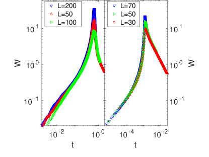
Figure 9: Time evolution of the roughness $W$ for the height profiles obtained in the Metropolis evolution of an Ising system in both, two and three-dimensional domains (left and right panels, respectively) with boundary conditions as described in Fig. 1 and for different values of the lateral system size $L$. All units are arbitrary.

References

- (1) M. Kardar, G. Parisi, and Y.-C. Zhang, Dynamic Scaling of Growing Interfaces, Phys. Rev. Lett. 56, 889 (1986).
- (2) G. Grinstein, Generic scale invariance and self-organized criticality, in Scale Invariance, Interfaces, and Non-Equilibrium Dynamics, edited by A. McKane, M. Droz, J. Vannimenus, and D. Wolf (Springer, Cambridge, England, 1995).
- (3) U. C. Täuber, Critical Dynamics (Cambridge University Press, Cambridge, England, 2014).
- (4) A.-L. Barabási and H. E. Stanley, Fractal concepts in surface growth (Cambridge University Press, Cambridge, England, 1995).
- (5) J. Krug, Origins of scale invariance in growth processes, Adv. Phys. 46, 139 (1997).
- (6) T. Kriecherbauer and J. Krug, A pedestrian’s view on interacting particle systems, KPZ universality and random matrices, J. Phys. A: Math. Theor. 43, 403001 (2010).
- (7) I. Corwin, The Kardar-Parisi-Zhang Equation and Universality Class, Random Matrices: Theor. Appl. 1, 1130001 (2012).
- (8) T. Halpin-Healy and K. A. Takeuchi, A KPZ Cocktail-Shaken, not Stirred…, J. Stat. Phys. 160, 794 (2015).
- (9) K. A. Takeuchi, An appetizer to modern developments on the Kardar-Parisi-Zhang universality class, Physica A 504, 77 (2018).
- (10) K. A. Takeuchi, M. Sano, T. Sasamoto, and H. Spohn, Growing interfaces uncover universal fluctuations behind scale invariance, Sci. Rep. 1, 34 (2011).
- (11) C. B. Mendl and H. Spohn, Dynamic correlators of Fermi-Pasta-Ulam chains and nonlinear fluctuating hydrodynamics, Phys. Rev. Lett. 111, 230601 (2013).
- (12) P. J. Yunker, M. A. Lohr, T. Still, A. Borodin, D. J. Durian, and A. G. Yodh, Effects of Particle Shape on Growth Dynamics at Edges of Evaporating Drops of Colloidal Suspensions, Phys. Rev. Lett. 110, 035501 (2013).
- (13) S. Nesic, R. Cuerno, E. Moro, Macroscopic response to microscopic intrinsic noise in three-dimensional Fisher fronts, Phys. Rev. Lett. 113, 180602 (2014).
- (14) S. N. Santalla, J. Rodríguez-Laguna, T. Lagatta, and R. Cuerno, Random geometry and the Kardar-Parisi-Zhang universality class, New J. Phys. 17, 33018 (2015).
- (15) S. N. Santalla, J. Rodríguez-Laguna, A. Celi, and R. Cuerno, Topology and the Kardar-Parisi-Zhang universality class, J. Stat. Mech. 023201 (2017).
- (16) L. Chen, C. F. Lee, and J. Toner, Mapping two-dimensional polar active fluids to two-dimensional soap and one-dimensional sandblasting, Nature Comm. 7, 12215 (2016).
- (17) P. A. Orrillo, S. N. Santalla, R. Cuerno, L. Vázquez, S. B. Ribotta, L. M. Gassa, F. J. Mompean, R. C. Salvarezza, and M. E. Vela, Morphological stabilization and KPZ scaling by electrochemically induced co-deposition of nanostructured NiW alloy films, Sci. Rep. 7, 17997 (2017).
- (18) E. Altman, L. M. Sieberer, L. Chen, S. Diehl, and J. Toner, Two-dimensional superfluidity of exciton polaritons requires strong anisotropy, Phys. Rev. X 5, 011017 (2015).
- (19) A. Nahum, J. Ruhman, S. Vijay, and J. Haah, Quantum entanglement growth under random unitary dynamics, Phys. Rev. X 7, 031016 (2017).
- (20) I. V. Protopopov, R. Samanta, A. D. Mirlin, and D. B. Gutman, Anomalous Hydrodynamics in a One-Dimensional Electronic Fluid, Phys. Rev. Lett. 126, 256801 (2021).
- (21) S. Gopalakrishnan and R. Vasseur, Kinetic Theory of Spin Diffusion and Superdiffusion in XXZ Spin Chains, Phys. Rev. Lett. 122, 127202 (2019).
- (22) M. Ljubotina, M. Žnidarič, and T. Prosen, Kardar-Parisi-Zhang Physics in the Quantum Heisenberg Magnet, Phys. Rev. Lett. 122, 210602 (2019).
- (23) J. De Nardis, S. Gopalakrishnan, R. Vasseur, and B. Ware, Stability of Superdiffusion in Nearly Integrable Spin Chains, Phys. Rev. Lett. 127, 057201 (2021).
- (24) L. Golubović and R. Bruinsma, Surface diffusion and fluctuations of growing interfaces, Phys. Rev. Lett. 66, 321 (1991).
- (25) R. Cuerno and K. B. Lauritsen, Renormalization-group analysis of a noisy Kuramoto-Sivashinsky equation, Phys. Rev. E 52, 4853 (1995).
- (26) S. M. A. Tabei, A. Bahraminasab, A. A. Masoudi, S. S. Mousavi, and M. R. Tabar, Intermittency of height fluctuations in stationary state of the Kardar-Parisi-Zhang equation with infinitesimal surface tension in d+1 dimensions, Phys. Rev. E 70, 031101 (2004).
- (27) A. Bahraminasab, S. M. A. Tabei, A. A. Masoudi, S. S. Mousavi, and M. R. Tabar, Zero tension Kardar-Parisi-Zhang equation in (d + 1)-dimensions, J. Stat. Phys. 116, 1521 (2004).
- (28) C. Cartes, E. Tirapegui, R. Pandit, and M. Brachet, The Galerkin-truncated Burgers equation: Crossover from inviscid-thermalized to Kardar-Parisi-Zhang scaling, Phil. Trans. R. Soc. A. 380 20210090 (2022).
- (29) E. Rodríguez-Fernández, S. N. Santalla, M Castro, and R. Cuerno, Anomalous ballistic scaling in the tensionless or inviscid Kardar-Parisi-Zhang equation, Phys. Rev. E (in press, 2022); arXiv:2205.08816 [cond-mat.stat-mech].
- (30) M. Schroeder, M. Siegert, D. E. Wolff, J. D. Shore, and M. Plischke, Scaling of growing surfaces with large local slopes, EPL 24, 563 (1993).
- (31) S. Das Sarma, S. V. Ghaisas, and J. M. Kim, Kinetic super-roughening and anomalous dynamic scaling in nonequilibrium growth models, Phys. Rev. E 49, 122 (1994).
- (32) J. M. López, M. A. Rodríguez, and R. Cuerno, Superroughening versus intrinsic anomalous scaling of surfaces, Phys. Rev. E 56, 3993 (1997).
- (33) J. J. Ramasco, J. M. López, and M. A. Rodríguez, Generic Dynamic Scaling in Kinetic Roughening, Phys. Rev. Lett. 84, 10 (2000).
- (34) D. Wei, A. Rubio-Abadal, B. Ye, F. Machado, J. Kemp, K. Srakaew, S. Hollerith, J. Rui, S. Gopalakrishnan, N. Y. Yao, I. Bloch, and J. Zeiher, Quantum gas microscopy of Kardar-Parisi-Zhang superdiffusion, Science 376, 716 (2022).
- (35) J. Asikainen, S. Majaniemi, M. Dubé, and T. Ala-Nissila, Interface dynamics and kinetic roughening in fractals, Phys. Rev. E 65, 052104 (2002).
- (36) J. Asikainen, S. Majaniemi, M. Dubé, J. Heinonen, and T. Ala-Nissila, Dynamical scaling and kinetic roughening of single valued fronts propagating in fractal media, Eur. Phys. J. B 30, 253 (2002).
- (37) H. Dashti-Naserabadi, A. A. Saberi, S. H. E. Rahbari, and H. Park, Two-dimensional super-roughening in the three-dimensional Ising model, Phys. Rev. E 100, 060101(R) (2019).
- (38) E. Rodríguez-Fernández, Ph.D. thesis, Universidad Carlos III de Madrid (unpublished) (2022).
- (39) B. Grossmann, H. Guo, and M. Grant, Kinetic roughening of interfaces in driven systems, Phys. Rev. A 43, 1727 (1991).
- (40) J. M. López, M. Castro, and R. Gallego, Scaling of Local Slopes, Conservation Laws, and Anomalous Roughening in Surface Growth, Phys. Rev. Lett. 94, 166103 (2005).
- (41) M. E. Newman and G. T. Barkema, Monte Carlo methods in statistical physics (Clarendon Press, Oxford, 1999).
- (42) J. Garcia-Ojalvo and J. M. Sancho, Noise in Spatially Extended Systems (Springer, Heildelberg, 1999).
- (43) S. Taverniers, F. J. Alexander, and D. M. Tartakovsky, Noise propagation in hybrid models of nonlinear systems: The Ginzburg-Landau equation, J. Comput. Phys. 262, 313 (2014).
- (44) J. Cardy, Scaling and Renormalization in Statistical Physics (Cambridge University Press, Cambridge, 1996).
- (45) K. Seshan and D. Schepis, Handbook of thin film deposition, (William Andrew, Amsterdam, 2018).
- (46) P. Meakin, Fractals, scaling and growth far from equilibrium (Cambridge University Press, Cambridge, UK, 1998).
- (47) M. Castro, R. Cuerno, A. Sánchez, and F. Domínguez-Adame, Anomalous scaling in a nonlocal growth model in the Kardar-Parisi-Zhang universality class, Phys. Rev. E 57, R2491 (1998).
- (48) M. Castro, R. Cuerno, A. Sánchez, and F. Domínguez-Adame, Multiparticle biased diffusion-limited aggregation with surface diffusion: A comprehensive model of electrodeposition, Phys. Rev. E 62, 161 (2000).
- (49) M. Nicoli, M. Castro, and R. Cuerno, Unified moving-boundary model with fluctuations for unstable diffusive growth, Phys. Rev. E 78, 021601 (2008).
- (50) M. Castro, R. Cuerno, M. Nicoli, L. Vázquez, and J. G. Buijnsters, Universality of cauliflower-like fronts: From nanoscale thin films to macroscopic plants, New J. Phys. 14, 103039 (2012).
- (51) J. M. Marcos, P. Rodríguez-López, J. J. Meléndez, R. Cuerno, and J. J. Ruiz-Lorenzo, Spreading fronts of wetting liquid droplets: Microscopic simulations and universal fluctuations, Phys. Rev. E 105, 054801 (2022).