Scattering Amplitude Techniques in Classical Gauge Theories and Gravity

by

Yilber Fabian Bautista Chivata

A Dissertation Submitted to
The Faculty of Graduate Studies
In Partial Fulfilment of the Requirements
for the Degree of
Doctor of Philosophy

Graduate Program in Physics
York University
Toronto, Ontario
July 2022

© Yilber Fabian Bautista Chivata, 2022

The following served on the Examining Committee for this thesis. The decision of the Examining Committee is by majority vote.

External Examiner:	Donal O’Connell
	Professor, School of Physics and Astronomy
	University of Edinburgh

Supervisor(s):	Sean Tulin
	Associate Professor, Department of Physics and Astronomy
	York University

Committee Members:	Matthew C Johnson
	Associate Professor, Department of Physics and Astronomy
	York University
	Associate Faculty, Perimeter Institute for Theoretical Physics
	Tom Kirchner
	Professor of Physics, Department of Physics and Astronomy
	York University

Internal-External Member:	EJ Janse van Rensburg
	Professor of Mathematics & Statistics, Department of Mathematics and Statistics
	York University

I hereby declare that I am the sole author of this thesis. This is a true copy of the thesis, including any required final revisions, as accepted by my examiners.

I understand that my thesis may be made electronically available to the public.

Statement of Contributions

Yilber Fabian Bautista was the sole author of chapter 2, chapter 8 as well as the Preliminaries chapter 1 and the general Introduction , which were not written for publication.

This thesis consists in part of five manuscripts written for publication, as well as current work in progress by the author and his collaborators.

1. Y.F. Bautista and A. Guevara: From Scattering Amplitudes to Classical Physics: Universality, Double Copy and Soft Theorems. [hep-th:1903.12419]

2. Y.F. Bautista and A. Guevara: On the Double Copy for Spinning Matter. JHEP 11 (2021) 184 [hep-th:1908.11349]

3. Y.F. Bautista, A. Guevara, C. Kavanagh and J. Vines: From Scattering in Black Hole Backgrounds to Higher-Spin Amplitudes: Part I. [hep-th:2107.10179]

4. Y.F. Bautista and N. Siemonsen: Post-Newtonian Waveforms from Spinning Scattering Amplitudes. JHEP 01 (2022) 006 [hep-th:2110.12537]

5. Y.F. Bautista and A. Laddha: Soft Constraints on KMOC Formalism. [hep-th:2111.11642]

6. Y.F. Bautista, A. Guevara, C. Kavanagh and J. Vines: From Scattering in Black Hole Backgrounds to Higher-Spin Amplitudes: Part II. In preparation.

7. Y.F. Bautista, A. Laddha and Y. Zhang: Subleading-Soft Constraints on KMOC Formalism. In preparation.

Each of the chapters of this thesis takes elements of the different manuscripts as follows:

Research presented in chapter 2 takes elements of works 1,3 and 5.

Research presented in chapter 3 is based in works 5 and 7.

Research presented in chapter 4 takes elements of works 1,3,4.

Research presented in chapter 5 is based in work 4.

Research presented in chapter 6 is based in work 2.

Research presented in chapter 7 takes elements of works 3 and 6.

Abstract

In this thesis we present a study of the computation of classical observables in gauge theories and gravity directly from scattering amplitudes. In particular, we discuss the direct application of modern amplitude techniques in the one, and two-body problems for both, scattering and bounded scenarios, and in both, classical electrodynamics and gravity, with particular emphasis on spin effects in general, and in four spacetime dimensions. Among these observables we have the conservative linear impulse and the radiated waveform in the two-body problem, and the differential cross section for the scattering of waves off classical spinning compact objects. Implication of classical soft theorems in the computation of classical radiation is also discussed. Furthermore, formal aspects of the double copy for massive spinning matter, and its application in a classical two-body context are considered. Finally, the relation between the minimal coupling gravitational Compton amplitude and the scattering of gravitational waves off the Kerr black hole is presented.

To Cindy:
                                                         For her unconditional support
                                                                 through the years we spent together.

Introduction

The more than 100 years old prediction made by Einstein for the existence of Gravitational Waves (GWs) [8], and the recent direct confirmation by the LIGO and VIRGO collaborations [9], started the so called era of gravitational wave astronomy. This new window into the universe not only allows us to test General Relativity (GR) to an unprecedented degree of accuracy, but also permits observational investigation of theories of modified gravity [10], while adding important new elements to the multi-messenger astronomy club, the latter of which aims to look for the existence physics beyond the standard model [11]. In a nutshell, GWs are perturbations of space and time that propagate through the universe carrying energy, linear and angular momentum which can be measured in terrestrial detectors. Since the first event detected by the LIGO collaboration in the fall of $2015$, an order of $100$ binary events have been subsequently detected including events from Binary Black Hole (BBH) [9], Binary Neutron Star (BNS)[12], and the more exotic, Black Hole-Neutron Star (BH-NS) system [13].

LIGO/VIRGO successful direct detection of GWs accounts for just the beginning of the gravitational wave era. Indeed, it is of common knowledge an upgrade of the LIGO/VIRGO detectors will take place within the next decade; this will be known as the era of the advance LIGO and VIRGO detectors, A+/Virgo+, and as a result, earth base gravitational wave instruments expect to observe an order of $10$ binary events every two weeks [14], increasing the statistical power in the measurement of classical gravitational observables in terrestrial detectors. Furthermore, the near future space-based LISA mission is expected to join the Gravitational-Wave (GW) instruments club in the couple of decades, bringing into the table access to binary merges of super massive black holes happening at large red-shift values ($z\sim 7$) [15]; such events will be further added to the BBH gravitational wave catalog. Additional GW observatories such as KAGRA [16], LIGO-India [17], the Einstein Telescope [18] and the Cosmic Explorer [19], will make of GW astronomy a highly active area of research in the coming decades. These will be instruments aiming to prove larger portions of the GW spectrum, ranging from frequencies of $10^{3}Hz$ (Sound frequencies) to $10^{-3}Hz$ (the m-sound ) .

In order to analyze data obtained from these different observatories, more refined theoretical predictions – which are the basis of GW templates production – will be needed. Traditionally, the production of GW template has been a collaborative effort that takes elements from Numerical Relativity (NR) [20], Black Hole Perturbation Theory (BHPT) and Gravitational Self-Force (GSF) [21, 22], the post-Newtonian (PN) formalism [23, 24] and the Effective One Body (EOB) method [25, 26, 27, 28]. More recently, however, efforts have been focused on the BBH scattering problem, in order to connect classical computations performed in the context of the Post-Minkowskian (PM) theory [29, 30, 31, 32, 33, 34, 35, 36, 37, 38, 39, 40, 41, 42], with those approaches based on the classical limit of Quantum Field Theory (QFT) scattering amplitudes [43, 44, 45, 46, 47, 48, 49, 50, 51, 52, 53, 54, 55, 56, 7, 57, 58, 59, 60, 61, 62, 63].

The theoretical predictions relevant for GW observatories fall into the category formed by the so called two-body. The two-body problem for coalescing compact objects – describing events such as those observed in LIGO/VIRGO detectors – is customary divided into three stages. The earliest one is known as the inspiral stage. This phase comprehends the majority of the coalescing process and is characterized by the non-relativistic motion of the binary components; in addition, the gravitational attraction between the two bodies falls into the weak regime which makes of perturbation theory a suitable candidate to deal with the problem. The next stage is the merge. In this phase the two body collapse due to their strong gravitational pull; the objects move with relativistic velocities and the problem becomes non-perturbative, making of NR the, so far, suitable tool to study the complex dynamics of the system. The final phase is known as the ring down, where a Kerr Black Hole (BH) is formed from the combination of the two coalescing compact bodies. This BH radiates GWs product of the excitation of its quasi-normal modes until a static configuration is reached. The main tool tho study this final stage is BHPT. See Figure 1 for a reconstruction example of the coalescing process for the first GW detection GW150914.

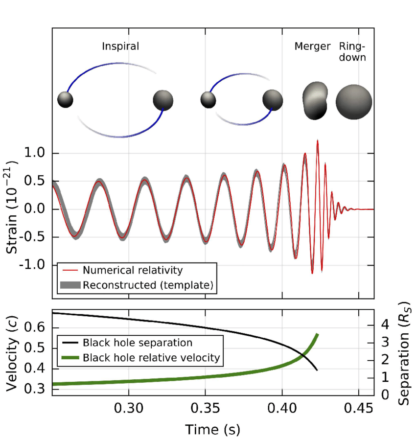
Figure 1: GW150914 signal interpretation as as seen at Hanford observatory. The three stages of the coalescing process are indicated. The lower plot shows the velocity of the components as function of their spatial separation. Figure reproduced from [2].

To be more precise, the let us consider in more detail several of the scales involved in the two-body problem. As already mentioned, a significant part of the observed GW signal is encapsulated by the inspiral phases where there are $\sim 10^{5}$ cycles for the two bodies going around each other. This makes the use of NR computationally expensive and therefore, analytic methods are more suitable to study such a phase. The traditional method to deal with such endeavor has been the PN formalism. It assumes both a weak field approximation (expanding in powers of $G$, the Newton constant, or more precisely $GM/c^{2}b$, with $b$ the separation between the bodies), as well as a non-relativistic approximation (expansion in powers of $v^{2}/c^{2}$, with $v$ the typical velocities of the coalescing bodies). The current state of art results for the two-body (conservative) dynamics is 5PN order [64] (See also Figure 3). Let us now imagine the scenario where one of the compact objects is much more massive than its companion, i.e. where the mass ratio condition $m_{1}/m_{2}\gg 1$ is satisfied. Systems with such a property are known as extreme mass ratio systems. A more suitable tool to study them is GSF, where the problem is effectively reduced to solve for the geodesic motion of the small massive object in the gravitational background field of its massive companion. One of the advantages of GSF over the PN approximation is that in principle GSF is non-perturbative in the sense it only assumes an expansion in powers of $m_{1}/m_{2}$, but can keep all orders in $G$ if desired, therefore accounting for parts of higher PN orders. See Figure 2 for typical systems where these methods are used. An alternative analytic approach to the two-body problem in the inspiral stage is provided by the PM approximation, which assumed the problem can be treated using an expansion in powers of $GM/c^{2}b$ only. In reality, this approach is more suitable for the scattering problem as opposite to the bounded orbits scenario. Nevertheless, since the PM approximation contains all powers in the velocity expansion, it naturally encapsulates PN information for the bounded scenario by means of the virial theorem $GM/c^{2}b=v^{2}/c^{2}$ (See Figure 3). PM methods include worldline and classical methods, as well as the more recent QFT approach as mentioned above. Let us finally mention the EOB method (now days enlarged by the Tutti-Frutti method [64]) is the formalism that allows to put together the information provided by the different approximations to the problem.

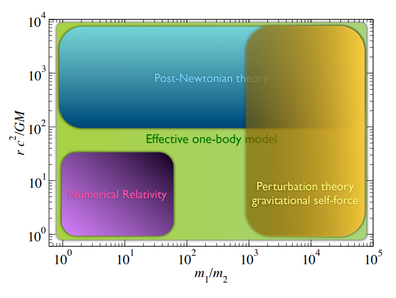
Figure 2: Validity of the different methods producing gravitational wave templates in a typical BBH system. Figure reproduced from [3].

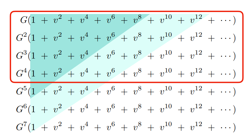
Figure 3: State of the art results for the GR two-body conservative potential. The horizontal lines in the red box indicate the state of the art PM results, whereas the vertical lines correspond then to the PN information currently available from PM methods. The dark blue triangle indicate the state of the art PM-PN overlap analytic information available for gravitational wave template production, whereas the light triangle indicates the required orders in $v$ and $G$, needed by future detectors. Figure reproduced from [4].

Of special interest for this thesis is the scattering amplitudes treatment of the two-body problem. This approach has recently gained attention since it provides with a scalable way of dealing with the two-body problem to very high orders in perturbation theory, while including spin [54, 57, 55] and tidal effects [65]. This is possible due to having at hand all of the QFT machinery developed for particle colliders such as double copy [66, 67], unitarity methods [51], leading singularity computations [7], the spinor helicity formalism [68], integration by parts identities [69, 70] and differential equations [71, 72, 73, 74, 75] for loop integration, among some others. This arsenal of tools makes of scattering amplitude methods a great candidate for hard core computations in gravity, and although these methods are valid only in scattering scenarios, extrapolations to bounded scenarios are partially understood [36, 37, 76]; we will get back to this in a moment.

At first it might seem a bit odd to use the QFT machinery to deal with problems which are of a purely classical nature. Let us however remember the correspondence principle states classical physics should emerge from quantum physics in the limit of large quantum numbers; that is, in the limit of macroscopic conserved charges such as mass, electric charge, orbital angular momentum, spin angular momentum, etc. In the context of the two-body problem, the transition from quantum to classical physics has been extensively studied [46, 77], and with the introduction of the Kosower, Maybee and O’connell (KMOC) formalism [78], a more precise map from the classical limit of scattering amplitude to classical observables in gauge theories an gravity has been established. Among the objectives of the amplitudes program in the two-body problem we have [4]:

• The production of state of the art predictions for the inspiral stage of the two-body problem in General Relativity and its possible modifications.

• Unraveling of hidden theoretical structures in the gravity, while looking for a scalable framework for computing classical observables beyond the inspiral phase.

• The connection of non-perturbative solutions in classical gravity, to perturbative scattering amplitudes realizations.

From a QFT setup, classical compact objects are understood as point particles dotted with a spin multipole structure. Additional finite size effects such as tidal deformability can be taken into account by including higher dimensional (non-minimal coupling) operators in the QFT description [65, 79]. Then, the amplitudes formulation of the two-body problem relies mostly (but not only) on the computation of the $2\to 2$ and $2\to 3$ scattering amplitudes for spinning massive particles interchanging and radiating gravitons:

(1)

The classical limit of these amplitudes are then associated to conservative and radiative effects in the two-body problem, respectively [80, 78]. These will be some of the main objects of study for the present thesis. Here it is precise to mention, for BHs, this Effective Field Theory (EFT) description can so far only account for physics happening away from the BH’s horizon. In fact, the amplitudes description of a Kerr BH actually describes a naked singularity rather than an actual BH, whose radius $a$, agrees with the spin vector of the Kerr BH [81]. This means dissipation effects at the horizon are yet to be understood in a QFT formulation of the problem, although there are already some hints from the classical worldline approach [82, 83, 40], as well as the amplitudes formulation of the scattering of waves off the Kerr BH [84, 85].

In practice, the two-body dynamics is studied in two separated sectors as given by the two amplitudes in (1): The first one corresponds to the conservative sector where not radiative effects are accounted for (although radiation reaction effects are encapsulated in the conservative amplitude). One of the greatest achievements from the amplitudes computation is the solution for the conservative dynamics at 4PM order (3 loops), for binary systems composed of scalar objects [86, 87], and at 2PM including spin effects up to quartic order [88], with recent new results at 3PM at the spin quadrupole level [89]. Preliminary results at 2PM but up to fifth [90] and seventh [91] order in spin have recently appeared. The second sector corresponds to the radiative sector which has into account radiation effects encoded in the energy and angular momentum emitted from the binary towards future null infinity in the form of GWs. The current state of art from the amplitudes approach to the radiative dynamics is 3PM order for scattering scenarios [92, 93, 94].

In the conservative sector, the transition from scattering to bounded systems can be made in several ways. Without a particular hierarchy, the first path one could take is by computing the Hamiltonian of the two-body system. The instantaneous potential for the gravitational interaction between the two bodies can be calculated for instance via a UV-EFT scattering amplitude matching procedure [44, 46], or via the scattering angle and the radial action [36, 37], or by using a relativistic Lippmann-Schwinger equation [49], or the spinor helicity variables in conjunction with the holomorphic classical limit [57, 55]. The second way for transitioning from scattering to bounded orbit systems is via a direct analytically continuation of the scattering observables [36, 37, 76].

The radiative sector is a bit more complicated. The traditional way of including radiation effects for coalescing compact objects in a Hamiltonian is via the EOB method. In this method, radiation reaction forces are included "by hand" in the particles Equations of Motion (EoM) [95]. This is an effect entering at the 2.5-PN order at the level of the EoM, and a 5-PN effect at the level of the radiated energy flux – one of the important radiation observable –. These terms added "by hand" in the EoM are dictated by balance equation [96], which have into account the lost of linear and angular momentum in the form of radiation emitted in the coalescing process. Once such terms are included in the EoM, they can also be added to the two-body Hamiltonian, the latter of which is the object used to compute all other observables for a given – bounded or unbounded – system. From an amplitude perspective, for the radiative dynamics, analytic continuation methods applied to scattering observables seem to still be valid when including radiation effects in the PM worldline EFT [97]. However, at 5PN order, back reaction makes non universal the unbounded and bounded problems, leading to non local in time terms; these are also known as tail terms [98, 99, 100], and it still needs to be understood how to account for them from an amplitudes approach. This then motivates to look for alternative continuation methods that can deal with the radiative bounded scenario directly from the scattering amplitudes. In this thesis we will take the first steps towards finding one of such methods, following the ideas of the authors in [101]; we will come back to this discussion below.

	GR	QED
quantum:	$\lambda_{c}\sim\frac{\hbar}{m}$	$\lambda_{c}\sim\frac{\hbar}{m}$
classical particle size:	$r_{S}=2GM$	$r_{Q}=\frac{e^{2}Q_{i}^{2}}{4\pi m}$
particle separation:	$b$	$b$

Table 1: Parameter comparison for the two-body problem in GR and electrodynamics. Here we have used units in which $c=1$. Table adapted from [1].

From the discussion above it might seen as if the amplitude methods are useful only for the two body problem in gravity. Let us take the opportunity to stress however, amplitude computations indeed extended beyond the two-body problem. In fact, with the introduction of the KMOC formalism, a variety of classical problems in gauge theories and gravity can now be approached from a pure QFT perspective. For instance, computation of related problems in classical electrodynamics as a toy model for gravity are now doable in a QFT setup [78, 102, 1, 92]. Perhaps the closest scenario to the discussion above is the relativistic two-body problem now in classical Electrodynamics. That is, one can compute classical observables for the relativistic scattering of two point-charges, in what is been called the post-Lorentzian (PL) expansion by the authors of ref. [1]. In Table 1 we have drawn a parallel of the relevant scales available for the two-body problem in GR and Electrodynamics, when approached from a QFT perspective. The scale controlling the quantum effects is the Compton wavelength of the participating particles $\lambda_{c}$, which is related to the Plank constant and the particle’s mass. The typical classical particle size $r_{S}$ and $r_{Q}$ corresponding to the Schwarzschild radius and charge radius, respectively. Finally, we have the particles separation $b$. Extracting classical information from a QFT scattering process in the PM approximation requires $\lambda_{C}\ll r_{S}\ll b$ as mentioned above. The first inequality corresponds to take the point particle limit, whereas the second inequality is equivalent to a large angular momentum expansion, which effectively permits to deal with the problem in a perturbative fashion. The electrodynamics analog to the PM expansion is then the PL expansion, which corresponds to the regime where $\lambda_{c}\ll r_{Q}\ll b$. Additional considerations have to be made when including radiation and spin effects. For the former, one requires the wavelength of the emitted wave to be much bigger than the size of the system; this in turn allows to recover the source multipole expansion for the radiation field. For the latter, combinations of the BH spin and the frequency of the emitted wave of the form $\omega a$ should remain finite. This then translates to take the large spin limit, as required by the correspondence principle.

Other problems in GR with immediate analog in classical electrodynamics include Gravitational and electromagnetic Bremsstrahlung radiation in a $2\to 3$ scattering process [78, 102, 1, 92]. The map of the 3-particle amplitude to the linearized effective Kerr metric [103, 58] and the root Kerr charge configuration [104], the Thomson scattering [105], and the scattering of waves off the Schwarzschild/Kerr black hole [84, 85] in bounded scenarios, the computation of the Maxwell dipole and the Einstein quadrupole radiation formulas directly from scattering amplitudes [31, 101] , the memory effect in gravity and electrodynamics [102, 106, 107], among some others. In this thesis we will approach several of these problems, with particular interests in spin effects both, in electrodynamics and in classical gravity.

Let us now take the opportunity to summarize the content of this thesis, while highlighting the contributions made by the author towards approaching some of the aforementioned problems. We however stress that if it is true a vast majority of the content of this thesis will be aimed to provide results relevant to the two-body problem, this thesis also aims to provide a more general understanding of the QFT description of purely classical problems, but at the same time, to provide some formal derivations in pure QFT scenarios, specially in the context of the double copy.

This thesis is organized as follows: In chapter 1 we present a preliminary compilation of several modern amplitude methods that are relevant for understanding the main body of this thesis. In particular, in section 1.2 we review the KMOC formalism in the context of the two body problem. This will provide us with a robust framework for computing observables in (classical) gauge theories and gravity directly from the (classical limit of) QFT amplitudes. In this section we provide a detail discussion on how to take the classical limit of QFT formulas in order to obtain the desired classical information. We focus on two main observables: The first one is the linear impulse acquired by a classical object in a $2\to 2$ scattering process, at generic order in perturbation theory. This observable is directly related to the scattering angle and therefore to the Hamiltonian of the system, as discussed above, so it is of main importance for the two-body problem. The second observable we discuss is the radiated classical electromagnetic/gravitational field in an inelastic $2\to 3$ scattering process, similarly, to generic order in perturbation theory. This will give us directly the waveform emitted from the scatter objects towards future null infinity. This waveform can be used to compute the (gravitational) wave energy flux, which is one of the main observables measured in a (gravitational) wave observatory. We then move to section 1.3 where we introduce some generalities of the Double copy for massless particles. In particular, we introduce the concept of Yang-Mills (YM) partial amplitudes and discuss their double copy formulation in the Kawai-Lewellen-Tye (KLT) form. We also discuss the color-kinematics duality and the Bern-Carrasco-Johansson (BCJ) formulation of the double copy of YM amplitudes. We provide simple examples for the double copy of the 3 and 4-point amplitudes. Understanding of the double copy for massless particles will be of special use when formulating the double copy for massive particles with spin, specially in chapter 4, chapter 6, and chapter 7. We move then to section 1.4 where we review the spinor helicity formalism for both massless and massive particles in 4 dimensions. We discuss the spinor helicity representation of massless and massive momenta, as well as polarization vectors. In the massless case we discuss how little group arguments fix completely the all helicity 3-point amplitude. In the massive case we discuss the exponential representation of the minimal coupling 3-point and the Compton amplitudes for spinning particles. Spinor-helicity variables will be of special use in chapter 6, chapter 7 and appendix B. We conclude in section 1.5 with a small outlook of the chapter.

Having acquired some preliminary knowledge of several of the modern amplitude techniques introduced in chapter 1, as a warm up in chapter 2 we begin the study of classical observables in Scalar Quantum Electrodynamics (SQED) from an amplitudes setup. This will provide some flavour on the amplitude formalism when dealing with classical observables, while avoiding the complications introduced by spin or higher Lorentz index structures. We start in section 2.2 by deriving from the SQED Lagrangian the three level amplitudes for a scalar matter line emitting one or two photons. We give this amplitudes special names $A_{n},\,\,n=3,4$, since they will be the building blocks for more complex amplitudes, as well as the topic of extensive studies in the proceeding chapters. We discuss immediate application of these amplitudes in a classical context. In particular, for $A_{3}$ we discuss how despite this being an amplitude with photon emissions, it does not carries any radiative content in Lorentz signature. For the case of $A_{4}$, we connect its classical limit to the Thomson scattering process in classical Electrodynamics (The analogous process in GR will be studied in chapter 7). Additional properties of these amplitudes such as soft exponentiation and the definition of orbit multipole moments are discussed. The latter correspond to the amplitude analog of the multipolar expansion in classical electrodynamics. It is then argue that $A_{4}$ has indeed non trivial orbit multipoles as opposite to $A_{3}$, which makes $A_{4}$ carry radiative degrees of freedom that $A_{3}$ does not possess. Soft exponentiation then allows us to argue these amplitudes can be derived directly from soft theorems and Lorentz invariance, without the need of a Lagrangian formulation. We move then to section 2.3 where a first application of the $A_{n}$ amplitudes in the two-body problem in SQED is introduced. At leading order in perturbation theory, we show how the classical content of the conservative and radiative two-body amplitudes is controlled by $A_{n}$ from the factorization properties:

(2)

These factorization properties are indeed more universal, and holds for spinning particles in both Quantum Electrodynamics (QED) and Gravity, which unify the computation of leading order radiation in classical electrodynamics and gravity in the compact formula (2.45). One can then obtain many of the physical features of the two-body problem from understanding the universality (and double copy ) properties of $A_{n}$ amplitudes. For instance, we show how the soft exponentiation of $A_{n}$ induces an all orders soft exponentiation of the two-body radiative amplitude, whose leading soft piece reproduces the memory waveform in SQED This memory waveform is universal (independent of the spin of the massive matter), for both QED and GR, as it is dictated only by the Weinberg soft theorem (In chapter 4 we argue how this universality can be seen from the spin multipole expansion for both QED and GR). We illustrate the computation of the leading order (section 2.3) and Next to leading order (section 2.4) classical impulse in a $2\to 2$ scattering process, using the KMOC formalism, and introducing some integration techniques that will be used in chapter 3. This allows us to shows how one can recover the classical result of Saketh et al [76] for the 2PL linear impulse, purely from amplitudes arguments. We also show how 3PL radiation results reproduce known classical results for colorless radiation computed from the worldline formalism by Goldberger and Ridgway [80]. Finally, we conclude in section 2.5 with an outlook of the chapter.

Continuing with the SQED theme, in chapter 3 we study low energy Bremsstrahlung radiation for the scattering two-body problem, from an amplitudes perspective. It is well known classical soft theorems predict the form of the wave emitted in a $N$-particle scattering process in the limit in which the frequency of the emitted wave is much smaller than the momenta of the other objects involved. Classical soft theorems are non perturbative statements and to prove them from perturbative approaches becomes a highly non-trivial task. However, they can also be used to probe perturbative approaches to the computation of classical radiation, in particular, on the KMOC formula for classical two-body radiation as discussed in chapter 1 and chapter 2. In this chapter we show that classical soft theorems impose an infinite series of constraints on KMOC formula. These constraints relate the expectation value of certain monomials of exchange momenta, to the linear impulse classical objects acquire due to the exchange of photons/gravitons in the scattering process, at arbitrary order in perturbation theory. We start in section 3.1 by reviewing some facts from classical soft theorems, and summarizing the main results of the chapter. Next we move to section 3.2 where we show explicit the prediction form classical soft theorem for the form of the radiated field in a $2\to 3$ scattering process to leading order in the soft expansion, and subleading order in perturbation theory. In section 3.3 we provide a formal derivation of the constraints imposed by the Weinberg soft theorem on the KMOC formula for the radiated field, which we then verify in section 3.4 up to Next to Leading Order (NLO) in the perturbative expansion, matching the expected results introduced earlier in section 3.2. In section 5.4 we provide an outlook of the chapter. Here we argue that although the soft constrains presented in this thesis were derived in the context of SQED , and to leading order in perturbation theory, analogous constraints follow for the gravitational case [107, 102], both at leading and subleading orders in the soft expansion [109]. In fact, in chapter 4 we show how the leading soft constrains in the gravitational context at Leading Order (LO) in perturbation theory recover the burst memory waveform of Braginsky and Thorne [110]. Soft theorem are non perturbative statements and in principle can inform about radiation to higher orders in perturbation theory, in fact, they are already used to compute radiation reaction effects in the high energy (eikonal) approximation of the two-body problem [53, 77, 111, 112]. Finally in appendix A we provide some computational details on the verification of the soft constraints at NLO in perturbation theory.

By then, the reader should had gained some familiarity with the amplitudes approach to obtaining classical physics from SQED. The natural thing to do next is to use the amplitude machinery to approach more complicated problems. There are several directions one could follow. For instance, one could introduce spin effects from QED, or study classical observables in gravitational physics involving scalar and spinning compact objects (minimally) coupled to gravity. These will be in fact the topics of study of chapter 4. Continuing the study of our favorite $A_{n}$ amplitudes, in section 4.2 we show when introducing spin effects, these amplitudes can be written in a spin multipole decomposition in generic spacetime dimensions. We differentiate two types of spin multipole moments: covariant, and rotation multipole. The former corresponds to irreducible representations (irreps.) of the Lorentz group in general dimension, SO$(D-1,1)$, whereas the latter are irreps. of the rotation subgroup SO$(D-1)$; these are the ones describing actual classical rotating objects. We compute the multipole decomposition for amplitudes involving particles of spin $0,\frac{1}{2},\,\,\text{and}\,\,1$, which are computed from the SQED , QED and Maxwell-Proca Lagrangians respectively. We show $A_{n}$ amplitudes can be written in terms of the Lorentz generators $J_{s}$ in the spin $s$ representation, with the multipole coefficients being universal functions (independent of the spin of the scattered particles). For $A_{3}$, we show how for spin $1/2$, QED predicts the electron ( tree level) gyromagnetic factor $g=2$, whereas for spin $1,$ the Proca Lagrangian predicts $g=1$ (We will revisit the $g$-factor in chapter 6, from double copy arguments, and argue $g=2$ for spin $1$ particles, where the massive vector particles are actually W-bosons). From unitary arguments, we show $A_{4}$ can be constructed from $A_{3}$ in a spin multipole form, with an exponential structure analog to the soft exponentiation of the scalar amplitude. These amplitudes can then be used to compute two-body observables in electrodynamics from the factorization properties (2). One can easily recover known linear in spin results [117]. In section 4.3 we introduce a covariant spin multipole double copy in generic space-time dimensions for the $A_{n}$ amplitudes. This double copy prescription has the property of preserving the spin multipole structure of the gravitational amplitudes, which can be used to compute two-body radiation from (2). This in turn implies leading order gravitational radiation can be computed from the double copy of photon radiation avoiding the complications form colour radiation. Using double copy arguments and universality of the coupling of matter to gravity, we show the 3-point amplitude for a massive spinning particle of generic spin takes an exponential structure (this exponential will be matched to the linearized Kerr metric in chapter 7). For the case of $A_{4}$ in gravity, we compute its covariant multipole decomposition up to quartic order in spin and show it agrees with the more lengthy Feynman diagrammatic computation from minimal coupling Lagrangians. We further decompose the Compton amplitude in terms of irreps. of SO$(D-1,1)$ by introducing the Ricci decomposition method, which allows to decompose the products of two Lorentz generators into the correspondent irreps. In order to make contact with actual classical rotating compact objects, we write the amplitudes in terms of the multipole moments for the rotation subgroup SO$(D-1)$. We show this is achieved by aligning spinning particles polarization tensors – which have different little group transformation properties – towards canonical polarizations with the same little group scaling for incoming and outgoing matter. This is done by fixing a condition on the spin tensor that goes by the name of the Spin Supplementary Condition (SSC) [118, 119]. This alignment also goes by the name of Hilbert space matching [56]. In $D=4$, we obtain up to quadratic in spin, a vector representation of the classical gravitational Compton amplitude, which has the property of factorizing into the product of the scalar amplitude and the spinning $s$-amplitude in QED, as dictated by the equivalence principle (In chapter 7 we show it reproduces results for Gravitational wave scattering off Kerr BH up to quadratic order in spin). Having understood the double copy properties of the $A_{n}$ amplitudes when including spin effects, as well as how to take their classical limit, in section 4.3.2 we show double copy of $A_{n}$ amplitudes induce a classical double copy formula for the two-body amplitudes (2), including spin effects. We use this formulas to compute radiation for scalar, linear and quadratic in spin, recovering known result in the literature [80, 6, 61, 117, 120]. In addition, we show for scalar matter an exponential soft theorem for the two-body radiation amplitude in gravity can be obtained, analog to the electromagnetic case of chapter 2, whose leading order allows to recover the memory waveform derived by Braginsky and Thorne [110]. We also show that spin effects in $M_{5}$ are subleading in the soft expansion, and therefore recovering the universality of the Weinberg soft theorem. We conclude in section 4.4 with an outlook of the chapter. In appendix B we provide some spinor helicity formulas to connect vectors results in this chapter to those given in spinor form in the literature.

In chapter 5 we do a transition from scattering to bounded scenarios. In particular, we show the inspiral waveform for two Kerr black holes orbiting in general (and quasi-circular orbits), whose spins are aligned with the direction of the system’s angular moment, and to leading and subleading order in the velocity expansion, can be obtained directly from the spinning amplitudes derived in chapter 4. Using an empiric formula for the waveform inspired by previous computations [121, 31], we propose such formula could modifies KMOC formula for the radiated field (1.18), to allow objects to move in generic trajectories. Particles EoM at leading order in velocity, but to all orders in spin, are analogously obtained from the conservative 4-point amplitude, via a modification of the KMOC formula for the linear impulse (1.12). We start this chapter in section 5.1 with a small introduction and summary of our results. We then move to section 5.2 where we provide a classical derivation of the gravitational waveform using the multipolar PM formalism [122, 123, 124, 125, 23]. In this section, we review the classical Lagrangian description of a spinning BH focusing on the conservative sector, where object’s EoM are derived, and provide explicit solutions to the EoM for the quasi-circular orbits scenario. We then use them into the multipolar expansion of the radiated field, obtaining solutions for the leading and subleading in velocity contributions to the waveform for binary systems in both, general and quasi-circular orbits, to all orders in spin. We move then to the amplitudes formulation of the problem in section 5.3. Introducing the general formalism, we write the formulas for the radiated field as well as particles equations of motion in terms of the non-relativistic limit of two-body scattering amplitudes. We review how to obtain the scalar waveform, reproducing the well known Einstein quadrupole radiation formula, and then provide spin corrections to it. For generic orbits, we show there is a one to one correspondence between the scalar amplitude and the source mass quadrupole moment, and in the same way, the linear in spin amplitude is in direct correspondence with the current quadrupole moment. We then show that at quadratic order in spin, and leading order in velocity, the radiated field acquires a vanishing contribution from the spin quadrupole radiation amplitude. The all orders in spin waveform at leading order in velocity is then obtained from the solutions to the particles EoM. We obtain the first subleading order in velocity correction to the quadrupole formula in the spinless limit, and show it agrees with the classical derivation obtained in section 5.2. We argue that although in general waveforms derived from different methods can differed one from the other by a time independent constant, physical observables such as the gravitational wave energy flux or the radiation scalar are insensitive to such a constant, as they can be computed from time derivatives of the waveform. This is a manifestation of a residual gauge freedom present in the waveform, which can be eliminated for physical observables. We conclude in section 5.4 with an outlook of the chapter. In appendix D we include some useful integrals and identities used for several computations in this chapter.

In chapter 6 we start a more formal study of the double copy for amplitudes involving massive spinning matter in generic space-time dimensions. In this chapter we aim to, on the one hand, provide a formal derivation of the double copy prescriptions introduced in chapter 4, and on the other hand, to derive the gravitational Lagrangians for the theories obtained from such double copies. We star in section 6.1 with a small introduction and a summary of the main results of the chapter. We argue double copy of spin $s$ with spin $\tilde{s}$ matter, leads to universal coupling of the resulting $(s,\tilde{s})$ massive particles to the graviton – as required by the equivalence principle – but in general the coupling to the dilaton and the two-form (axion) potential are not universal. For interactive spin 1 particles in gravity, this allows us to define two independent gravitational theories which we name the $0\otimes 1$ and the $\frac{1}{2}\otimes\frac{1}{2}$ theories. We provide general dimension tree-level Lagrangians in the Einstein frame for one and two spinning matter lines. Theory $\frac{1}{2}\otimes\frac{1}{2}$ is a simpler theory as compared to the $0\otimes 1$ counterpart, since on the one hand, it does not include quartic terms in the two matter lines Lagrangian, and on the other hand, one can consistently truncate the double copy spectrum to remove the coupling of matter to the two-form potential. On the other hand, in $D=4$ and in the massless limit, the $0\otimes 1$ theory reproduces the bosonic interaction of $\mathcal{N}=4$ Supergravity, which arises from the double copy $\mathcal{N}=4$ Super Yang-Mills and YM theories. In general dimensions, this theory is the QFT version of the worldline double copy model constructed by Goldberger and Ridgway in [80, 32] and extended to include spin effects in [31, 117]. In section 6.2 we derive the massive double copy formulas, for the theories consider, from dimensional reduction and compactification of the massless counterparts. We provide a variety of examples of amplitudes derived from such double copy formulas for one matter line emitting radiation. Furthermore, we show explicitly how to obtain the multipole double copy prescription introduced in chapter 4 from these dimensionally reduced double copy formulas. In the same section we discuss how setting $g=2$ for the gyromagnetic factor removes the divergences of the Compton amplitude in the massless limit. Such amplitude coincides with the minimal coupling Compton amplitude written in spinor helicity variables in section 1.4. We continue in section 6.3 where we construct massive Lagrangians both for Quantum Chromodynamics (QCD) and the gravitational theories from Kaluza-Klein (KK) reduction and compactification. For spin 1 in QCD, we introduce a modification of the Proca Lagrangian to set $g=2$ which is characteristic of the W-boson. We then show that QCD amplitudes $A_{n}$ for generic $n$, entering in the double copy formulas derived in section 6.2, are obtained from the compactification of their massless counterpart. This is the reason these amplitudes possessa well defined high energy limit. In section 6.3.2 we derive the Lagrangians for one matter line for the $0\otimes 1$ and $\frac{1}{2}\otimes\frac{1}{2}$ gravitational theories. In section 6.4 we study the massive double copy construction for spinning amplitudes including two matter lines. We use the massive version of the BCJ prescription introduced in section 1.3, providing the two-matter lines gravitational Lagrangians for the different double copy prescriptions. For inelastic scattering, we probe there is a Generalized Gauge Transformation that allow to recover the classical double copy formula for the radiation amplitude obtained from the factorization (2), this time directly from the quantum BCJ double copy. We finalize in section 6.5 with an outlook of the chapter. In section E.1 we prove our general dimensional $\frac{1}{2}\otimes\frac{1}{2}$ gravitational Lagrangian agrees with the $D=4$ derivation obtained in [126]. In section E.2 we study the unitarity properties of the $\frac{1}{2}\otimes\frac{1}{2}$ amplitudes at four points.

Up to this point, we would have claimed the classical limit of amplitudes for massive spinning matter minimally couple to gravity actually describes the Kerr BH. Perhaps the strongest hint is given by the computation of the waveforms for bounded systems described in chapter 5. However, the spin structure of the non-relativistic waveforms derived there follows mostly from $A_{3}$ whose classical limit now days is well known encode all the spin multipoles of the linearized Kerr metric. The natural question to ask is whether $A_{4}$ has actually anything to do with Kerr. In chapter 7 we show that $A_{4}$ is indeed very related to Kerr as it describes the low energy regime for the scattering of gravitational waves off the Kerr BH. We start this chapter with a small introduction and a summary of the results in section 7.1. We stress finding the connection of $A_{n}$ amplitudes to Kerr is important since they are the building blocks for the two-body amplitudes. In particular, it is important to prove the 2PM scattering angle for aligned spin computed in [58] actually describes the scattering of two Kerr BHs and not other classical compact objects. In section 7.2 we show how to take the classical limit of $A_{n}$ amplitudes written in spinor helicity form. For $n=3$ we indeed recover the Linearized Kerr metric, whereas for $n=4$, up to quartic order in spin, the gravitational Compton amplitude can be written in an exponential form for both, same and opposite helicity configurations of the external graviton legs, in agreement with the classical heavy particle effective theory derivation of [60]. In section 7.2.2 we use $A_{4}$ amplitude to study the scattering of gravitational waves off Kerr, obtaining the differential cross section for generic spin orientation of the BH, recovering the linear in spin results of [127] for polar scattering. Spin induced polarization of the waves is discussed in section 7.2.3, which to linear order in spin recovers the BHPT results of [127] and therefore clarifying the mismatch from the Feynman diagrammatic computation of [128, 129]. The solution of the discrepancy comes by including all the Feynman diagrams contributing to the Compton amplitude and not just the graviton exchange diagram, as done by the authors in [128, 129] [128, 129]. The quartic in spin result for the differential cross section provides a highly non-trivial prediction, pushing the linear in spin state of the art result of [127] since 2008, while providing a way to resum the partial infinite sums appearing from BHPT for generic orientation of the spin of the BH. In appendix F we provide a detail derivation of the differential cross section up to quartic order in spin from BHPT, finding perfect agreement with the amplitudes computation, therefore showing the Compton amplitude indeed possessthe same spin multipole structure as that of the Kerr BH when perturbed by a gravitational wave. In section 7.3 we show the classical limit of the Compton amplitude derived in here indeed can be used to compute the 2PM aligned spin scattering angle for the scattering of two Kerr BHs, therefore confirming the validity of the predictions of [58]. We close with an outlook of this chapter in section 7.4.

We finalize this thesis with at general discussion in chapter 8.

Chapter 1 Prelimimaries

1.1 Introduction

In this chapter we will introduce some aspect of scattering amplitudes that will be of great use for the present thesis. We start in section 1.2 reviewing some features of the KMOC formalism [78], which is a robust frame for the computation of (classical) observable directly from the (classical limit of the) scattering amplitudes. In this thesis we will be interested in 2 KMOC observables: 1) The linear impulse in a $2\to 2$ elastic scattering process, and 2) The radiated field at future null infinity from a $2\to 3$ inelastic scattering process. This section will be of great use for most of the content of the present thesis, specially for chapter 2,chapter 3, chapter 4. In chapter 5 we motivate a modification of KMOC formalism to study two-body systems for bounded orbits. Next, we move to section 1.3 where we introduce some general aspects of the double copy [66, 67]. In particular, we focus on the massless double copy of Yang Mills amplitudes in both, the KLT and the BCJ representations. Intuition from the massless double copy will be of great use when formulating double copy prescriptions for massive particles with and without spin, presented in chapter 4 and chapter 6. Finally, in section 1.4 we introduce the spinor-helicity formalism for massless and massive particles. In particular, we will review how helicity arguments fix the 3 and 4 point amplitudes for massive/massless spinning particles. Knowledge of this formalism will be of great use through several chapters of this thesis, in particular when discussing higher spin amplitudes in chapter 7.

1.2 The Kosower, Maybee and O’Connell formalism (KMOC)

In this section we start by introducing the KMOC formalism. As already mentioned, the KMOC formalism [78, 130, 59, 131, 132, 93], provides us with a robust framework for the computation of (classical) observables in gauge theories and gravity, directly from (the classical limit of ) QFT scattering amplitudes. It has become one of the cornerstone in the amplitude program in classical physics, and is directly relevant to understand the content of this thesis. In this formalism, classical compact objects are described in an effective way as point particles, whose finite size effects can be mapped into intrinsic properties of the elementary particles used in the EFT description. In what follows we review some of the most relevant aspects of this formalism. For a nice review, the reader is recommended to consult the original KMOC work, as well as the recent reference [133].

In the KMOC formalism, the expectation value for the change of a quantum mechanical observable, $\Delta\hat{\mathcal{O}}$, due to a scattering process is computed from the scattering matrix through the formula

$$\Delta\hat{\mathcal{O}}=\,_{\rm{in}}\langle\Psi|S^{\dagger}\hat{\mathcal{O}}S|\Psi\rangle_{\rm{in}}-\,_{\rm{in}}\langle\Psi|\hat{\mathcal{O}}|\Psi\rangle_{\rm{in}}\,,$$ (1.1)

This corresponds to the difference of the measurement of the given operator in the final and initial state, where we have relied on $S$ as a time evolution operator determining the form of the asymptotic final state of the system $\ket{\Psi}_{\text{out}}=S\ket{\Psi}_{\text{in}}$. The connection of $\Delta\hat{\mathcal{O}}$ to the a QFT scattering amplitude is done in two steps: First, we need to split the $S$-operator in the usual way, $S=1+iT$, after which, exploding the unitarity condition, $SS^{\dagger}=1$, allows us to rewrite (1.1) in the form:

$$\Delta\hat{\mathcal{O}}=\,_{\rm{in}}\langle\psi|[T,i\hat{\mathcal{O}}]|\Psi\rangle_{\rm{in}}+\,_{\rm{in}}\langle\psi|T^{\dagger}[\hat{\mathcal{O}},T]|\Psi\rangle_{\rm{in}}\,.$$ (1.2)

Second, we need to specify the system’s initial state. For the moment let us assume it can be decompose into multi-particle plane wave states, which in momentum space are proportional to $\ket{p_{1},\cdots,p_{n}}$. These states are the tensor product of individual momentum eigenstates $a_{p}^{\dagger}\ket{0}$, where $a_{p}^{\dagger}$ is the creation operator for state of momentum $p$. The conjugate states are labeled by $\bra{p_{1}^{\prime},\cdots p_{m}^{\prime}}$, and together with $T$, define the QFT scattering amplitude via

$$\mathcal{A}(p_{1},\cdots,p_{n}\to p_{1}^{\prime},\cdots,p_{m}^{\prime})\hat{\delta}^{d}(p_{1}+\cdots p_{n}-p_{1}^{\prime}-\cdots p_{m}^{\prime})=\bra{p_{1}^{\prime},\cdots,p_{m}^{\prime}}T\ket{p_{1},\cdots,p_{n}}\,.$$ (1.3)

where $\hat{\delta}^{d}(p_{1}+\cdots p_{n}-p_{1}^{\prime}-\cdots p_{m}^{\prime})$ is the momentum conserving delta function in general dimension (we will specialize to $d=4$ in several parts of this thesis below, for the moment let us keep the generic dimension approach).

The extraction of classical information in this formalism has two main ingredients to be taken in mind: 1) A parameter that controls the classical expansion, and 2) The choice of suitable wave functions describing the multi-particle initial state of the system. For the former, it is natural to use $\hbar$ as the parameter that controls the classical expansion. It appears in two main places in the computations: First, in the coupling constants, which by reintroducing $\hbar\neq 1$, are to be re-scaled via $g\to g/\sqrt{\hbar}$, and second, the wave numbers associated to massless momenta for the force carriers, which are introduced as $q=\hbar\bar{q}$. We will discuss in detail below how to extract the classical limit of (1.2), as well as the choice of suitable on-shell initial state, for a given observable. For the moment, the classical classical piece $\langle\mathcal{O}\rangle$ of the observable, can be formally defined as

$$\langle\Delta\hat{\mathcal{O}}\rangle=\lim_{\hbar\to 0}\hbar^{\beta_{\mathcal{O}}}\left[\,{}_{\rm{in}}\langle\Psi|[T,i\hat{\mathcal{O}}]|\Psi\rangle_{\rm{in}}+\,_{\rm{in}}\langle\Psi|T^{\dagger}[\hat{\mathcal{O}},T]|\Psi\rangle_{\rm{in}}\,\right]\,,$$ (1.4)

here $-\beta_{\mathcal{O}}$ is the power of the LO-piece in the $\hbar$-expansion of the quantities inside the square brackets, which depends on the specific observable, as well as on the theory considered. Then, the factor of $\hbar^{\beta_{\mathcal{O}}}$ in this formula then ensures $\langle\mathcal{O}\rangle\sim\hbar^{0}$, i.e. classical scaling. For instance, for the radiated photon field, we have $\beta_{\mathcal{O}}=\frac{3}{2}$, whereas for the linear impulse we use $\beta_{\mathcal{O}}=1$.

In this thesis we are interested in two observables: 1) The conservative linear impulse $\langle\Delta\hat{p}\rangle$ (a global observable, i.e. independent of the particles positions), acquired by classical compact objects in a $2\to 2$ scattering process in Electrodynamics/Gravity. 2) The classical radiated electromagnetic/gravitational field $\langle\hat{A}^{\mu}\rangle/\langle\hat{h}^{\mu\nu}\rangle$ (a local "observable", i.e. dependent on the particles positions ) in a non-conservative $2\to 3$ scattering process.

1.2.1 Linear impulse in $2\to 2$ scattering

At the classical level, the linear impulse dictates the total change in the momentum of one of the particles after the scattering process. At the quantum level, the impulse corresponds to the difference between the expected outgoing and the incoming momenta of such particle, as given by the KMOC formula (1.4). For this observable it is convenient to choose the initial state of the system $|\Psi\rangle_{\text{in}}$, as follows

$$|\Psi\rangle_{\text{in}}=\int\prod_{i}\big{[}\hat{d}^{d}p_{i}\hat{\delta}^{(+)}(p_{i}^{2}-m_{i}^{2})\phi_{i}(p_{i})e^{ib_{i}{\cdot}p_{i}/\hbar}\big{]}|p_{1}p_{2}\rangle$$ (1.5)

where we have employed the notation of the original reference [78], however, unlike for the original work, and to be more general, we have move to a frame where both particles are displaced by the positions $b_{i}$, with respect to such reference frame. Then, the difference $b_{2}-b_{1}=b$, corresponds then to the impact parameters, which is the distance of closest approach between the particles during the scattering process. Notice $|\Psi\rangle_{\text{in}}$ is built from on-shell states, of positive energy, as dictated by $\hat{\delta}^{(+)}(p_{i}^{2}-m_{i}^{2})=(2\pi)\delta(p_{i}^{2}-m_{i}^{2})\Theta(p^{0})$ , there $\Theta(x)$ is the heaviside step function. $\phi_{i}(p_{i})$, corresponds to relativistic wave functions associated to the incoming massive particles, whose classical limit shall result into the point particle description of the compact objects. We will come on this below.

The system’s initial states is assumed to be normalized to the unit $\,{}_{\text{in}}\langle\psi|\psi\rangle_{\text{in}}=1$. From this, it follows the normalization condition for the wave functions,

$$\int\hat{d}\Phi_{i}(p_{i})|\phi_{i}(p_{i})|^{2}=1\,.$$ (1.6)

Here we have written the on-shell phase-space measure as $d\Phi(p_{i})=\hat{d}^{d}p_{i}\hat{\delta}^{+}(p_{i}^{2}-m_{i}^{2})$.

The next task is to relate the observable (1.4) to the scattering amplitude using (1.3), together with the initial two-particle state (1.5). Notice in general the computation of an observable will have the contribution of two terms, one which is linear in the amplitude, whereas the second one is quadratic. This is in general true to all orders in perturbation theory, except for the leading order, where the latter is subleading. Let us for the moment focus on the contribution linear in the amplitude. At $(n)$-order in perturbation theory it reads explicitly

$$I_{(1)}^{(n)\,\mu}=\int d\Phi(p_{1},p_{2})d\Phi(p_{1}^{\prime},p_{2}^{\prime})\phi_{1}(p_{1})\phi_{2}(p_{2})\phi_{1}^{*}(p_{1}^{\prime})\phi_{2}^{*}(p_{2}^{\prime})i(p_{1}^{{}^{\prime}\mu}-p_{1}^{\mu})e^{i(p_{1}{\cdot}b_{1}+p_{2}{\cdot}b_{2})}\bra{p_{1}^{\prime}p_{2}^{\prime}}T\ket{p_{1}p_{2}}^{(n)}$$ (1.7)

Here we have used $\hat{p}_{i}\ket{p_{i},p_{j}}=p_{i}\ket{p_{i},p_{j}}$, and $d\Phi(p_{i},p_{j})=d\Phi(p_{i})d\Phi(p_{j})$. In addition, we have labeled the conjugate states with primed variables as mentioned above. Next we can replace $\bra{p_{1}^{\prime}p_{2}^{\prime}}T\ket{p_{1}p_{2}}$ in terms of the scattering amplitude as given by (1.3), this will introduce a $d$-fold delta function that will allow us to perform $d$-integrals in the previous formula. Introducing the momentum miss-match $q_{i}=p_{i}^{\prime}-p_{i}$, and changing the integration variables from $p_{i}^{\prime}\to q_{i}$, and further using the momentum conserving delta function to do perform the integration in $q_{2}$, followed by the relabel $q_{1}\to q$, (1.7) becomes

$$\begin{split}I_{(1)}^{(n)\,\mu}&=\int d\Phi(p_{1},p_{2})\hat{d}^{d}q\hat{\delta}(-2p_{1}{\cdot}q+q^{2})\hat{\delta}(2p_{2}{\cdot}q+q^{2})\Theta(p_{1}^{0}+q^{0})\Theta(p_{2}^{0}-q^{0})\\ &\qquad\qquad\qquad\phi_{1}(p_{1})\phi_{1}^{*}(p_{1}-q)\phi_{2}(p_{2})\phi_{2}^{*}(p_{2}+q)iq^{\mu}e^{-iq{\cdot}b}\mathcal{A}^{(n)}(p_{1},p_{2}\to p_{1}-q,p_{2}+q)\end{split}$$ (1.8)

Before discussing how to take the classical limit of this expression, let us analyze the analogous expression for the term quadratic in the amplitude, entering in the KMOC formula (1.4). Since there are two factors of $T$ in this term, we need to introduce a complete set momentum eigenstates between the two factors of $T$ in such way we can extract a momentum eigenvalue when the momentum operator hits the momentum eigenstates. At $(n)$ order in perturbation this can be done as follows

$$\begin{split}I_{(2)}^{(n)\,\mu}&=\sum_{X=0}^{n-1}\int\prod_{m=0}^{X}d\Phi(r_{m})\prod_{i=1}^{2}d\Phi(R_{i})d\Phi(p_{i})d\Phi(p_{i}^{\prime})\phi_{i}(p_{i})\phi_{i}^{*}(p^{\prime}_{i})e^{ip_{i}{\cdot}b_{i}}(R_{1}^{\mu}-p_{1}^{\mu})\\ &\times\sum_{a=0}^{n-1-X}\bra{p_{1}^{\prime},p_{2}^{\prime}}T\ket{R_{1},R_{2},r_{X}}^{(a)}\bra{R_{1},R_{2},r_{X}}T^{\dagger}\ket{p_{1}p_{2}}^{(n-a-X-1)}\,,\end{split}$$ (1.9)

Here we have used $\hat{p_{1}}\ket{R_{1},R_{2},r_{X}}=R_{1}\ket{R_{1},R_{2},r_{X}}$, where $r_{X}$ represent additional massless states propagating through the cut. They only appear at sub-sub-leading (two loops) order in perturbation theory. We now proceed in an analogous way to the linear in amplitude computation, that is. we need to replace the dependence of the scattering amplitude via (1.3). Defining the momentum mismatch $q_{i}=p_{i}^{\prime}-p_{i}$, as well as the momentum transfer $w_{i}=R_{i}-p_{i}$, allows us to change the integration variables $p_{i}^{\prime}\to q_{i}$ and $R_{i}\to w_{i}$. In addition, we can use the momentum conserving delta function for each amplitude to perform the integration in $q_{2}$ and $w_{2}$, which followed by the relabeling $w_{1}\to w$ and $q_{1}\to q$ results into

$$\begin{split}I_{(2)}^{(n)\,\mu}&=\sum_{X=0}^{n-1}\int\hat{d}^{d}w\hat{d}^{d}q\prod_{m=0}^{X}d\Phi(r_{m})\prod_{i=1}^{2}d\Phi(p_{i})\hat{\delta}(-2p_{1}{\cdot}q+q^{2})\hat{\delta}(2p_{2}{\cdot}q+q^{2})e^{-iq{\cdot}b}w^{\mu}\\ &\hat{\delta}(-2p_{1}{\cdot}w+w^{2})\hat{\delta}(2p_{2}{\cdot}w+w^{2})\phi_{1}(p_{1})\phi_{1}^{*}(p_{1}-q)\phi_{2}(p_{2})\phi_{2}^{*}(p_{2}+q)\\ &\times\Theta(p_{1}+w)\Theta(p_{2}-w)\Theta(p_{1}+q)\Theta(p_{2}-q)\\ &\times\sum_{a_{1}=0}^{n-1-X}\mathcal{A}^{(a_{1})\,\mu}(p_{1},p_{2}{\rightarrow}p_{1}{-}w,p_{2}{+}w,r_{X})\,,\\ &\times\mathcal{A}^{(n-a_{1}-X-1)\star}(p_{1}{-}w,p_{2}{+}w,r_{X}{\rightarrow}p_{1}-q,p_{2}+q)\end{split}$$ (1.10)

This is the analog to (1.8). With these two contributions at hand, the quantum mechanical impulse particle 1 acquires during the scattering process, at $(n)$-order in perturbation theory is simply given by the sum

$$\Delta p_{1}^{\mu}=I_{(1)}^{(n)\,\mu}+I_{(2)}^{(n)\,\mu}$$ (1.11)

Classical limit

We now proceed to extract the classical piece in the QM-impulse (1.11). This is done through a series of steps: 1) The factors of $\hbar$ are restored in the formulas through the rescaling of the coupling constant $g\to g/\sqrt{\hbar}$ and the massless momenta $q\to\bar{q}\hbar$ and $w\to\bar{w}\hbar$. 2) There are 3 length scales to consider in the problem. The first one is defined by the size of massive particles, given by the Compton wavelength $\lambda_{c}=\hbar/m$ (which in the classical context traduces to the radius of the classical charge/Black hole given by $r_{Q}=e^{2}Q^{2}/(4\pi m)$ / or $r_{S}=2GM$). The second scale corresponds to the spread of the relativistic wave function $l_{s}$, and third, the separation between the particles $b$. In the classical limit, the following approximation should hold $\lambda_{c}\ll l_{s}\ll b$, which holds true if $b$ scales as $b\to b/\hbar$. The first part of the inequality simply imposes the effective point particle description of the classical objects, the second on the other hand ensures a non-overlapping of the particles’ wave functions (typical of the long range scattering in classical physics), finally, the approximation $\lambda_{c}\ll b$ in the classical context becomes $e^{2}Q^{2}/4(\pi m)\ll b$ the Post-Lorentzian (PL) approximation, which allows us to compute observables order by order in perturbation theory (In the gravitational context this is $2GM\ll b$, which corresponds to the PM approximation ). 3) In the case in which there is the emission of external radiation (as will be the case for the waveform emission), the massless momenta of the photon/graviton need to also be re-scaled analogously as $k\to\bar{k}\hbar$. This is equivalent to ask for long wavelength radiation (which in the bounded system scenario allows to recover the source multipole expansion).

After this considerations, the previous discussion is equivalent to approximate the wave functions $\phi_{i}(p_{i}+\hbar\bar{q})\approx\phi_{i}(p_{i})$, followed by a Laurent-expansion of all of the components of the integrands, in powers of $\hbar$. At this stage, the explicit dependence of the wavefunction can be integrated out, leaving us with the classical observable

$$\begin{split}\langle\Delta p_{1}^{(n)\,\mu}\rangle&=\lim_{\hbar\to 0}\Big{[}\int\hat{d}^{d}q\hat{\delta}(-2p_{1}{\cdots}q+q^{2})\hat{\delta}(2p_{2}{\cdots}q+q^{2})iq^{\mu}e^{-iq{\cdot}b}\mathcal{A}(p_{1},p_{2}\to p_{1}-q,p_{2}+q)\\ &+\sum_{X=0}^{n-1}\int\hat{d}^{d}w\hat{d}^{d}q\prod_{m=0}^{X}d\Phi(r_{m})\hat{\delta}(-2p_{1}{\cdot}q+q^{2})\hat{\delta}(2p_{2}{\cdot}q+q^{2})e^{-iq{\cdot}b}w^{\mu}\hat{\delta}(-2p_{1}{\cdot}w+w^{2})\hat{\delta}(2p_{2}{\cdot}w+w^{2})\\ &\times\sum_{a_{1}=0}^{n-1-X}\mathcal{A}^{(a_{1})\,\mu}(p_{1},p_{2}{\rightarrow}p_{1}{-}w,p_{2}{+}w,r_{X})\times\mathcal{A}^{(n-a_{1}-X-1)\star}(p_{1}{-}w,p_{2}{+}w,r_{X}{\rightarrow}p_{1}-q,p_{2}+q)\Big{]}\end{split}$$ (1.12)

As mentioned, in general we will have to Laurent-expand in $\hbar$ both, the on-shell delta functions, as well as the reduced amplitudes. At leading order $(n=0)$, only the term linear in the amplitude contributes to the impulse, in that case we can drop the $q^{2}$ factor inside the delta functions, since no singular terms in $\hbar$ appear in the amplitude. However, at higher orders in the perturbative expansion, possible singular terms arise in the amplitude. This singular terms are expected to be cancelled between the linear and quadratic in amplitudes terms. In chapter 3 we will see and explicit example of this cancellation. There is however no formal proof this cancellation happens to any order in perturbation theory.

We conclude then that the classical linear impulse is controlled basically by the (n)-Loop 4-point amplitude $\mathcal{A}(p_{1},p_{2}\to p_{1}-q,p_{2}+q)$, as well as the $4+X$-cut amplitudes from the iterated piece.

1.2.2 The radiated field in $2\to 3$ scattering

We now move to the analysis of the computation of the radiated photon/graviton field in a $2\to 3$ scattering process. This will be analog to the previous example, whit a few interesting features arising from the non-conservative dynamics. Here we will be interested in computing the expectation value of the photon/graviton field operator $\hat{A}^{\mu}(x)/\hat{h}^{\mu\nu}(x)$. This unlike the case for the impulse is a local observable, depending on the position $x$ at which the field is measured. In particular, we are interested in the asymptotic for of the radiated field at future null infinity, which scales as $1/R$, with $R=|\vec{x}|$. This scaling follows naturally from the mode integration of the field operator. In what follows we focus on the electromagnetic case, but the results can be easily generalized to the gravitational case.

We want to compute the expectation value of the field operator, whose mode expansion is

$$\hat{A}^{\mu}(x)=\text{Re}\sum_{\eta=\pm 1}\int d\Phi(k)\epsilon_{\eta}^{\mu}e^{-ik{\cdot}x}a_{\eta}^{\dagger}(k)$$ (1.13)

here the sum over $\eta$ is a sum over the photon polarization, and $a_{\eta}^{\dagger}(k)$ are creation operators for photons of momentum $k$ and helicity $\eta$. The next step is to put this operator inside our favorite KMOC formula (1.4). Since this is a $2\to 3$ scattering process, we can reuse (1.5) as our two-particle initial state. Although no initial radiation is present in the initial state, $a_{\eta}^{\dagger}(k)$ creates a particle of momentum $k$ and helicity $\eta$, when acting on the conjugate states $\bra{p_{1},p_{2}^{\prime},k_{\eta}}$.

We then have as usual two contributions to the radiated field. The first one linear in the amplitude, however, since there is the creation of such massless momenta state, the controlling amplitude in this case at $(n)$-Loop order is the 5-point amplitude $\mathcal{A}(p_{1},p_{2}\to p_{1}-q_{1},p_{2}-q_{2},k_{\eta})$. Analogously, the quadratic in amplitude part will be controlled by the $5+X$-amplitudes as shown below. At this stage, the classical limit outlined in previous section can be implemented straightforwards. This in turn integrates out the dependence on the particles wave functions, leaving us with an expression analog to (1.12), inside the radiated photon phase space. That is, writing the radiated field in (1.13) as an effective source integrated over the massless photon phase space,

$$\langle\hat{A}^{\mu}(x)\rangle=\text{Re}\int d\Phi(k)e^{-ik{\cdot}x}\langle J^{\mu}(k)\rangle$$ (1.14)

where the angular brackets indicate the classical limit has been taken. At $(n)$-order in perturbation theory, we naturally identify the source as given by the sum of two terms as follows

$$\langle J^{(n)\,\mu}(k)\rangle=\mathcal{R}^{(n)\,\mu}(k)+\mathcal{C}^{(n)\,\mu}(k),$$ (1.15)

which have the explicit recursive form

$$\mathcal{R}^{(n)\,\mu}(k)=i\lim_{\hbar\to 0}\hbar^{\frac{3}{2}}\int\prod_{i=1}^{2}\hat{d}^{4}q_{i}\hat{\delta}(2p_{i}{\cdot}q_{i}-q_{i}^{2})e^{ib_{i}{\cdot}q_{i}}\hat{\delta}^{4}(q_{1}{+}q_{2}-k)\mathcal{A}^{(n)\,\mu}\left(p_{1},p_{2}{\rightarrow}p_{1}{-}q_{1},p_{2}{-}q_{2},k\right)\,,$$ (1.16)

and

$$\begin{split}\mathcal{C}^{(n)\,\mu}(k)&={\color[rgb]{0,0,0}}\lim_{\hbar\to 0}\hbar^{\frac{3}{2}}\sum_{X=0}^{n-1}\int\prod_{m=0}^{X}d\Phi(r_{m})\prod_{i=1}^{2}\hat{d}^{4}w_{i}\hat{d}^{4}q_{i}\hat{\delta}(2p_{i}{\cdot}q_{i}{-}q_{i}^{2})\hat{\delta}(2p_{i}{\cdot}w_{i}{-}w_{i}^{2})e^{ib_{i}{\cdot}q_{i}}\\ &\hskip 56.9055pt\,\,\,\,\,\,\,\,\,\,\,\,\times\hat{\delta}^{4}(w_{1}{+}w_{2}{+}r_{X}{-}k)\hat{\delta}^{4}(w_{1}{+}w_{2}{+}r_{X}{+}q_{1}{+}q_{2})\\ &\hskip 56.9055pt\,\,\,\,\,\,\,\,\,\,\,\,\,\times\sum_{a_{1}=0}^{n-1-X}\mathcal{A}^{(a_{1})\,\mu}(p_{1},p_{2}{\rightarrow}p_{1}{-}w_{1},p_{2}{-}w_{2},r_{X},k)\\ &\hskip 56.9055pt\,\,\,\,\,\,\,\,\,\,\,\,\,\times\mathcal{A}^{(n-a_{1}-X-1)\star}(p_{1}{-}w_{1},p_{2}{-}w_{2},r_{X}{\rightarrow}p_{1}-q_{1},p_{2}-q_{2})\,,\end{split}$$ (1.17)

where the $\star$ in one of the amplitude indicates complex conjugation. We refer to the $\mathcal{C}^{(n)\,\mu}(k)$ term as the cut-box contribution, to indicate that it is given by the cut of higher loop amplitudes. In this expression, $r_{X}$ denotes the collection of momenta $\{r_{1},\cdots,r_{X}\}$ carried by additional particles propagating thorough the cut, whose momentum phase space integration has been explicitly indicated by $d\Phi(r_{m})=\hat{d}^{4}r_{m}\hat{\delta}^{(+)}(r_{m}^{2})$. For $n=0\,\,\rm{and}\,\,1$, no additional photons propagate thought the cut, since they only appear starting from $\rm{N}^{2}$LO in the perturbative expansion (i.e. two-loops).

$\langle J^{(n)\,\mu}(k)\rangle$ can then be interpreted as a classical source entering into the RHS of the field equations, and is computed directly from the scattering amplitudes. It is particularly remarkable how the classical field is controlled by single photon emission amplitudes, while the classical field should be composed from many photon. In [134], it was shown such amplitudes parametrize the high photon occupation number as expected for a classical field. An analogous expression for the source in the gravitational case $\langle T^{(n)\,\mu\nu}(k)\rangle$ follows from the scattering amplitudes. The difference is in the double Lorentz index characterizing the graviton polarization tensor.

In this thesis we will mostly be interested in the computation of the previous source in both, the electromagnetic and the gravitational case. We do not perform explicitly the photon/graviton phase space integration in (1.14) although a simple proof can be found in the review [133]. Here we just mention the integration in $k$ can be made in an almost independent way from the amplitude. The result is then to just bring down a power of $R$ in the denominator which ratifies the radiative nature of the classical field. There is additional exponential factor from the retarded nature of the radiation. In $d=4$ one can show (1.14) becomes

$$\langle\hat{A}^{\mu}(x)\rangle=\frac{1}{4\pi R}\text{Re}\int d\omega e^{-i\omega T_{R}}\langle J^{\mu}(\omega,\hat{n})\rangle$$ (1.18)

where we have used $k=\omega(1,\hat{n})$, with $\hat{n}=\vec{x}/R$, is the unit direction of emission of the radiation, and $T_{R}=t-R$ is the retarded time.

1.3 A few worlds on the double copy

Let us now move to study some generalities of the so called double copy of scattering amplitudes. The program of the double copy originally started from the observation by KLT in [135] that $n$-point tree-level closed string scattering amplitudes can be computed from the sum of products of n-point open string partial amplitudes, with coefficients that depend on the kinematic variables. This program has however seen many incarnations, ranging from perturbative QFT realizations [67], to the understanding the double copy structure of non perturbative solutions classical gravity [136, 137, 138, 139, 140, 141, 142, 143, 104] . The double copy colloquially goes by the slogan GR = YM², which is the simple observation that amplitudes involving massless gravitons in GR can be directly obtained from products of amplitudes for the scattering of gluons in non abelian gauge theories. Currently, we understand the double copy is much more general feature of QFT amplitudes [144, 145], and is naturally realized in classical sectors as well. Indeed, in this thesis we will learn how to connect classical and quantum versions of the double copy, including spinning massive particles chapter 6.

In the remaining of this section we give a brief introduction to the computation of GR amplitudes from the double copy of their YM counterparts. For that, let us first recall the color decomposition of YM amplitudes, it will be useful when studying the KLT formulation of the double copy below.

Color Decomposition

n-gluon scattering amplitudes can be factorized into two pieces. The firs piece contains the information of the color structure, whereas the second one containing only kinematics information of the scattering process. This factorization is known as color decomposition of gauge theory amplitudes [146, 147]. More precisely, for $n$-external gluon legs, the tree level $n$-point scattering amplitude is written in terms of $(n-1)!$ single-trace color structures as follows:

$$\mathcal{A}^{\text{tree}}(g_{1},\cdots,g_{n})=\sum_{\sigma\in S_{n-1}}\text{tr}(T^{a_{1}}T^{a_{\sigma_{2}}}\cdots T^{a_{\sigma_{n}}})A(1,\sigma_{2},\cdots,\sigma_{n})\,.$$ (1.19)

The sum here runs over non-cyclic permutations of the indices $\{1,2,\cdots,n\}$, corresponding to the set of inequivalent traces, and $T^{a_{n}}$ are the gauge group generators in the adjoint representation. We have use cyclic invariance of the trace to fix one of the entries. $A(1,\sigma_{2},\cdots,\sigma_{n})$ are known as partial amplitudes or color ordered amplitudes , and are gauge invariant [149] objects, depending only on the momenta and polarization vectors of the particles in the scattering process. They are computed from the Feynman diagrams that respect the order of the momentum labels (in other words, planar diagrams), using Feynman rules that respect such a order [148].

Since there is only $(n-1)!$ independent color factors, these partial amplitude basis is over completed. Indeed, partial amplitudes satisfy linearly constraints that allow us to reduce the number of independent elements to $(n-2)!$. These constraints are known as Kleiss-Kuijf relations [150, 151], the simplest of which is the U($1$) decoupling identity

$$A(1,2,3,\cdots,n)+A(1,3,2,\cdots,n)+\cdots+A(1,3,\cdots,n,2)=0,$$ (1.20)

which follows from the $T^{a}\to 1$ replacing of the generators in (1.19). See [152] for a discussion of the additional relations. Kleiss-Kuijf relations are not the only constraints on the partial amplitudes, indeed, there are additional relations known as the BCJ relations [67], which impose a series of constraints that reduces the number of independent partial amplitudes to $(n-3)!$. Let us stress here the choice of partial amplitudes basis is not unique since we could have chosen any other pair of legs in replacement of the reference legs $1,n$, in (1.19).

1.3.1 KLT representation of the double copy

Now that we understand the concept of partial amplitudes, we are ready to present a first form of the double copy of YM amplitudes, this is the KLT form of the double copy. It says $n$-point axio-dilaton-gravity scattering amplitudes can be obtained from the sum of two copies of $n$-point partial YM amplitudes. More precisely

$$A_{n}^{\text{GR}}=\sum_{\alpha\beta}K_{\alpha\beta}A^{\text{YM}}(1,\cdots,n)\bar{A}^{\text{YM}}(1,\cdots,n)$$ (1.21)

The sum over $\mbox{$\alpha$},\,\beta$ ranges over $(n-3)!$ orderings, corresponding to the number of independent partial amplitudes, and $K_{\alpha,\beta}$ is the standard KLT kernel [135, 153, 154]. Let us emphasise formula (1.21) is valid in general space-time dimensions. Notice in addition, as natural from string theory, a graviton state come accompanied by an antisymmetric tensor $B^{\mu\nu}$, and a scalar, the dilaton. Amplitudes computed using (1.21) have therefore these additional states in the spectrum. We will see a more detailed discussion of this fact in section 4.3.

Let us provide a simple example of how to use formula (1.21). The simplest double copy amplitude is indeed given for the $n=3$ case. The partial amplitude for the scattering of 3-gluons, with momentum conservation $p_{1}-p_{2}+p_{3}=0$, and $p_{i}{\cdot}\epsilon_{i}=\epsilon_{i}^{2}=0$, is simply given by

$$A^{\text{YM}}_{3}(1,2,3)=2g(p_{1}{\cdot}\epsilon_{3}\epsilon_{1}{\cdot}\epsilon_{2}-p_{1}{\cdot}\epsilon_{2}\epsilon_{1}{\cdot}\epsilon_{3}+p_{3}{\cdot}\epsilon_{1}\epsilon_{2}{\cdot}\epsilon_{3})\,.$$ (1.22)

Formula (1.21) allows us to compute the 3-graviton scattering amplitude in general dimensions, and is given by the squaring of this simple amplitude. The KLT kernel at three-points is simply $K_{3}=\kappa/(4g^{2})$. We can choose graviton polarization tensors to be given $\epsilon_{i}^{\mu\nu}=\epsilon_{i}^{\mu}\epsilon_{i}^{\nu}$.

$$A_{3}^{\text{GR}}=\kappa(p_{1}{\cdot}\epsilon_{3}\epsilon_{1}{\cdot}\epsilon_{2}-p_{1}{\cdot}\epsilon_{2}\epsilon_{1}{\cdot}\epsilon_{3}+p_{3}{\cdot}\epsilon_{1}\epsilon_{2}{\cdot}\epsilon_{3})^{2}\,.$$ (1.23)

See chapter 6 for a discussion on how to obtain amplitudes for dilaton scattering.

As a further example we can compute the 4-graviton scattering amplitude from the double copy of the 4-gluon scattering amplitude. In this case there is also one independent partial YM amplitude, say $A^{\text{YM}}_{4}(1,2,3,4)$, which for momentum conservation $p_{1}+p_{2}=p_{3}+p_{4}$ is simply given by

$$\begin{split}A^{\text{YM}}_{4}(1,2,3,4)=\frac{2g^{2}\epsilon_{1,\alpha}\epsilon_{2,\beta}}{p_{1}{\cdot}p_{3}\,p_{1}{\cdot}p_{4}}\big{[}p_{1}{\cdot}p_{3}F_{4}^{\mu\alpha}F_{3,\mu}^{\beta}{+}p_{1}{\cdot}p_{4}F_{3}^{\mu\alpha}F_{4,\mu}^{\beta}{+}F_{3}^{\alpha\beta}p_{1}{\cdot}F_{4}{\cdot}p_{2}{+}F_{4}^{\alpha\beta}p_{1}{\cdot}F_{3}{\cdot}p_{2}{+}p_{1}{\cdot}F_{3}{\cdot}F_{4}{\cdot}p_{1}\eta^{\alpha\beta}\big{]}\,.\end{split}$$ (1.24)

Here we have used $F_{i}^{\mu\nu}=2p_{i}^{[\mu}\epsilon_{i}^{\nu]}$. In this case, the 4-graviton scattering amplitude in general dimension is simply

$$A^{\text{GR}}_{4}=K_{4}A^{\text{YM}}_{4}(1,2,3,4)^{2}\,,$$ (1.25)

where the 4-point KLT kernel is simply $K_{4}=\frac{p_{1}{\cdot}p_{3}p_{1}{\cdot}p_{4}}{8g^{4}p_{3}{\cdot}p_{4}}$.

1.3.2 The BCJ representation of the double copy

We have seen how the KLT formula (1.21) allows us to compute GR amplitudes in a straightforward manner. The formula however becomes quite non-trivial to use when the number of external legs become big, this because we will have, as seen, $(n-3)!$ independent partial amplitudes to compute. On the other hand, this formula is only valid for tree-level amplitudes. In this subsection we introduce a different representation of the double copy that overcomes these problems. This is the BCJ [67] double copy formulation, which is one of the main computational tools in the modern amplitudes program in gravity [144].

The Color-Kinematic duality

The BCJ form of the double copy was originated from the following observations: A given $n$-point YM amplitude can always be written in the following fashion

$$A_{n}^{\rm{YM}}=g^{n-2}\sum_{\Gamma}\frac{c_{i}n_{i}}{d_{i}}\,,$$ (1.26)

where the sum run over trivalent graphs, $d_{i}$ are kinematic denominators contains physical poles, and are made of ordinary scalar Feynman propagators, $c_{i}$ encode the color structure and $n_{i}$ are kinematics numerators. For a given triplet $(i,j,k)$, the color factors satisfy the Jacobi identity

$$c_{i}\pm c_{j}=\pm c_{k}\,,$$ (1.27)

then the numerators can be arrange in such a way they satisfy an analog kinematic relation

$$n_{i}\pm n_{j}=\pm n_{k}\,.$$ (1.28)

This is relation is known as the color-kinematic duality.

The BCJ proposal is then that gravitational amplitudes can be computed by replacing the color factors $c_{i}$ by a second copy of kinematics numerators $\tilde{n}_{i}$ as follows

$$A^{\rm{GR}}=\sum_{\Gamma}\frac{n_{i}\tilde{n}_{i}}{d_{i}}\,.$$ (1.29)

The two gauge theories can in general be different, and only one of theme is required to satisfy the color-kinematic duality (1.28) in order for the gravitational amplitude (1.29) to be gauge invariant [155, 156].

Let us remark although originally this formulation was done in the massless YM sector, it has been extended to include both massless and massive matter, including spin effects. We will revisit this formulation in chapter 6 in the context of spinning matter. Also, there is analogous formulation of the BCJ double copy at higher orders in perturbation theory [144].

Let us as an example recompute the 4-graviton scattering amplitude (1.25) using the BCJ double copy formula (1.29). For this case, the YM amplitude has the contribution of 3 color structures, as associated to each of the graphs in Figure 1.1.

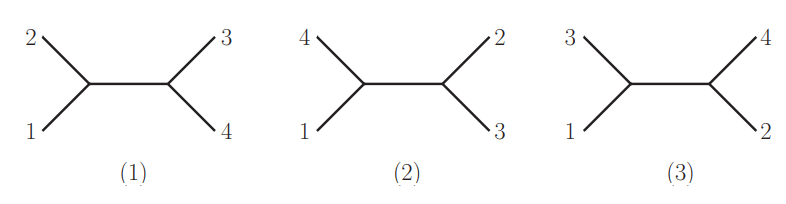
Figure 1.1: Feynman diagrams that contribute to the 4-gluon amplitude in the BCJ representation. Figure adapted from [5]

The $s-$channel color factor is simply given by the contraction of the colour structure constant associated to each 3-vertex

$$c_{s}=f^{a_{1}a_{2}b}f^{ba_{3}a_{4}}\,.$$ (1.30)

The corresponding numerator is

$$n_{s}=\Big{[}\epsilon_{1}{\cdot}\epsilon_{2}p_{1}^{\mu}+2\epsilon_{1}{\cdot}p_{2}\epsilon_{2}^{\mu}-(1\leftrightarrow 2)\Big{]}\Big{[}\epsilon_{3}{\cdot}\epsilon_{4}p_{3}^{\mu}+2\epsilon_{3}{\cdot}p_{4}\epsilon_{4}^{\mu}-(3\leftrightarrow 4)\Big{]}+s\Big{[}\epsilon_{1}{\cdot}\epsilon_{3}\,\epsilon_{2}{\cdot}\epsilon_{4}-\epsilon_{1}{\cdot}\epsilon_{4}\,\epsilon_{2}{\cdot}\epsilon_{3}\Big{]}$$ (1.31)

The additional numerators follow from index-relabeling as in Figure (1.1). It is easy to show the color factors satisfy (1.27), as it is just the usual Jacobi identity for the structure constants of the gauge group. Explicit computation also shows the numerators satisfy the analog relation (1.28), and can therefore be used in (1.29) to compute the 4-graviton amplitude, which will agree with the KLT result (1.25).

We have then two alternative constructions for the double copy, which we will explore further through the body of this thesis.

1.4 The spinor-helicity formalism

In this final section we introduce the spinor-helicity formalism, which is convenient to use when dealing with observables in $4$ spacetime dimensions. This formalism is based on the simple observation that spin-1 vectors transforms as $(\frac{1}{2},\frac{1}{2})$ representations of the Lorentz group in $4$ spacetime dimensions and can therefore be represented as a bi-spinors, where each component acts on its respective $\frac{1}{2}$ representation. Naturally, particles momenta $p^{\mu}$ are Lorentz vectors, and can indeed be represented in this spinorial form $p^{\alpha\dot{\alpha}}$. There is a distinction however between massive and massless momenta which we need to take into account.

Recall under Wigner’s classification [159], particles correspond to irreducible, unitary representations of the Poincare group. In this sense, massless and massive particles are fundamentally different and need to be distinguished when written in their spinorial form. This is because they have associated different little group. Remember the little group is defined as the set of Lorentz transformations that leave particles momenta invariant. Each particle has its own little group. For instance, for massless particles we can choose a frame in which the momentum vectors are of the form $p^{\mu}=\omega(1,0,0,1)$, and therefore the little group corresponds to the group of rotations in the x-y plane, SO$(2)=$U$(1)$. For massive particles on the other hand, one can choose the particle’s rest frame where $p^{\mu}=(m,0,0,0)$. This allow us to identify the little group as the three-spatial rotations group SO$(3)\sim$SU$(2)$.

With this distinction between massless and massive particles in mind, let use introduce their correspondent spinor helicity formalism in a separate way. For the former we follow the conventions of [160] (see also [152]), whereas for the latter we follow the seminal work in [68].

1.4.1 Massless particles

The transition from the vector to the spinorial representation of particle’s momenta is done thought the su($2$) sigma matrices $\sigma^{\mu}=(\mathbb{I},\sigma^{i})$, via

$$p^{\alpha\dot{\alpha}}=\sigma_{\mu}^{\alpha\dot{\alpha}}p^{\mu}=\left(\begin{array}[]{cc}p^{0}-p^{3}&-p^{1}+ip^{2}\\ -p^{1}-ip^{2}&p^{0}+p^{3}\end{array}\right)$$ (1.32)

in this matrix notation, the on-shell condition becomes

$$p^{2}=\det(p^{\alpha\dot{\alpha}})=p_{0}^{2}-p_{1}^{2}-p_{2}^{2}-p_{3}^{2}=0\,,$$ (1.33)

The two-dimensional momentum matrix $p^{\alpha\dot{\alpha}}$ has therefore rank 1 and can be written as the outer product of two vectors

$$p^{\alpha\dot{\alpha}}=\lambda^{\alpha}\tilde{\lambda}^{\dot{\alpha}}\,.$$ (1.34)

$\alpha$ and $\dot{\alpha}$ are SU($2$) indices, which can be raised and lower with the invariant $\epsilon$-tensor

$$\epsilon^{\alpha\beta}=-\epsilon_{\alpha\beta}=\epsilon^{\dot{\alpha}\dot{\beta}}=-\epsilon_{\dot{\alpha}\dot{\beta}}=\left(\begin{array}[]{cc}0&1\\ -1&0\end{array}\right)\,.$$ (1.35)

A possible parametrization of these spinors in terms of the momentum vector components is

$$\lambda^{\alpha}=\frac{z}{\sqrt{p^{0}-p^{3}}}\left(\begin{array}[]{c}p^{0}-p^{3}\\ -p^{1}-ip^{2}\end{array}\right)\,,\,\,\,\,\,\,\,\tilde{\lambda}^{\dot{\alpha}}=\frac{z^{-1}}{\sqrt{p^{0}-p^{3}}}\left(\begin{array}[]{cc}p^{0}-p^{3}&-p^{1}+ip^{2}\end{array}\right)$$ (1.36)

with $p^{0}=\sqrt{p_{1}^{2}+p_{2}^{2}+p_{3}^{2}}$. Notice we have include a general scaling constant $z$. This is because under the little group transformation, $\lambda\to z\lambda$ and $\tilde{\lambda}\to z^{-}1\lambda$, the matrix $p^{\alpha\dot{\alpha}}$ remains invariant. For real kinematics $\lambda^{\alpha}=(\tilde{\lambda}^{\dot{\alpha}})^{\dagger}$ and therefore the factor $z$ becomes a pure phase. $z=e^{i\phi}$. For Complex momenta, $\lambda$ and $\tilde{\lambda}$ are unrelated one to the other.

We can analogously defined the conjugate matrix $\bar{p}_{\dot{\alpha}\alpha}=(\bar{\sigma}^{\mu})_{\dot{\alpha}\alpha}p^{\mu}$, with $\bar{\sigma}^{\mu}=(\mathbb{I},-\sigma^{i})$. It is furthermore convenient to introduce the bracket notation $\lambda_{p}^{\alpha}=\ket{p}$ and $\tilde{\lambda}_{p}^{\dot{\alpha}}=[p|$ to represent the spinor-helicity variables. In this way the momentum matrices become

$$p^{\alpha\dot{\alpha}}=\ket{p}[p|\,,\qquad\bar{p}_{\dot{\alpha}\alpha}=|p]\bra{p}.$$ (1.37)

In this notation, the Lorentz product of two vectors, $p$ and $q$, becomes

$$2p{\cdot}q=\text{tr}(\bar{p}q)=\text{tr}(\bar{q}p)=\text{tr}(|p]\bra{p}\ket{q}[q|)=\braket{pq}[qp]=\braket{qp}[pq]\,.$$ (1.38)

Here we have denoted the contractions $\braket{pq}=\lambda_{p}^{\alpha}\lambda_{q}^{\beta}\epsilon_{\alpha\beta}$, and analogously $[pq]=\tilde{\lambda}_{p}^{\tilde{\alpha}}\tilde{\lambda}_{q}^{\dot{\beta}}\epsilon_{\dot{\alpha}\dot{\beta}}$. This implies $\braket{pq}=-\braket{qp}$ and $[pq]=-[qp]$, and therefore, for any massless momentum $p$, we have $\braket{pp}=[pp]=0$.

Non surprisingly, massless polarization vectors (as well as Dirac spinors) can also be put into a spinorial form. Recall they satisfy the transversality condition $\epsilon{\cdot}p=0$. This condition allows us to write positive and negative helicity polarizations matrices in terms of the spinors for their associated massless momentum as follows

$$\epsilon_{p}^{-}=\sqrt{2}\frac{\ket{p}[r|}{[pr]}\,,\qquad\epsilon_{p}^{+}=\sqrt{2}\frac{\ket{r}[p|}{\braket{rp}}\,,$$ (1.39)

here $\ket{r}$ and $[r|$ are two reference spinors (when computing amplitudes, they cancel out from the final answer), whose freedom to be chosen is the manifestation of the gauge freedom one has to shifting massless polarization vectors, with vectors proportional to their correspondent momentum $\epsilon_{\mu}\to\epsilon_{\mu}+\frac{\sqrt{2}}{[pr]}p_{\mu}$, in a physical scattering amplitude. Notice polarization vectors defined in (1.39) carry little group weights. That is, under a little group transformation, $\epsilon^{-}\to z^{2}\epsilon^{-}$ and $\epsilon^{+}\to z^{-2}\epsilon^{+}$. Finally, polarization vectors satisfy the usual conditions $\epsilon_{p}^{-}{\cdot}\epsilon_{p}^{+}=-1$, and $\epsilon_{p}^{\pm}{\cdot}\epsilon_{p}^{\pm}=\epsilon_{p}^{\pm}{\cdot}p=0$.

Any scattering amplitude in 4-dimensions can be written in terms of inner products of spinor-helicity variables. Since reference spinors are little group invariant, the little group rescaling of an amplitude is fixed only by the external polarizations. This impose strong constrains on the permitted form of an amplitude, since arbitrary inner products of spinors must have the correct little group rescaling in order for the amplitude to describe the desired scattering process. Indeed, in [161] it was shown that for complex momenta, on-shell 3-particle S-matrices of massless particles of any spin can be uniquely determined from helicity arguments. This is where the power of the spinor helicity formalism overcomes the use of usual polarization tensors. That is, for a given particle of any spin, the spin structure is completely contained in the spinors $\{\ket{p},|p]\}$. We will see this is also the case for massive spinning particles in section 1.4.2.

Massless 3-point amplitude

For the 3-point amplitude of massless particles with generic spin (or helicity $h=s$), and momentum conservation $p_{1}+p_{2}+p_{3}=0$, $p_{i}^{2}=0$, with $p_{i}{\cdot}p_{j}=0$, Lorentz invariance impose the amplitude to be generic function of spinorial combinations $\braket{ij}$ and $[ij]$, with $i,j=1,2,3$. At 3-points, the most generic function is split into a holomorphic and anti-holomorphic contributions [161]:

$$A_{3}(\{i,h_{i}\})=\kappa_{H}\braket{12}^{d_{3}}\braket{23}^{d_{1}}\braket{31}^{d_{2}}+\kappa_{A}[12]^{-d_{3}}[23]^{-d_{1}}[31]^{-d_{2}}\,,$$ (1.40)

where $\kappa_{h},\kappa_{A}$ are constant coefficients and

$$d_{1} =h_{1}-h_{2}-h_{3}$$ (1.41)

$$d_{2} =h_{2}-h_{3}-h_{1}$$ (1.42)

$$d_{3} =h_{3}-h_{1}-h_{2}$$ (1.43)

Imposing $A_{3}(\{i,h_{i}\})$ has correct physical behaviour in the limit of real kinematics ($\braket{ij}=0$ and $[ij]=0$), implies that if $d_{1}+d_{2}+d_{3}>0$, one needs to set $\kappa_{A}=0$, and analogously if $d_{1}+d_{2}+d_{3}>0$ then $\kappa_{H}=0$. In this work we consider $d_{1}+d_{2}+d_{3}\neq 0$ only, as for zero sum, the two contributions need to be kept.

As an example, we can compute the 3-point amplitude for a massless state of helicity $h$ emitting a massless particle of spin $h_{3}$:

$$A_{3}^{h_{3},h}\sim\left(\frac{\langle 13\rangle}{\langle 23\rangle}\right)^{2h}\left(\frac{\langle 13\rangle\langle 32\rangle}{\langle 12\rangle}\right)^{h_{3}},$$ (1.44)

We will come back to this amplitude in chapter 6 and chapter 7.

1.4.2 Massive particles

Let us now introduce the spinor helicity formalism for massive particles. We have learned that massless particles are labeled by their helicity weight, $h$. Massive particles on the other hand transform under some spin $S$ representation of SU$(2)$. The transition from vector to spinors notation can be done analogously to the massless case (1.32). Since the on-shell condition for massive particles is $p^{2}=m^{2}$, the matrix $p^{\alpha\dot{\alpha}}$ is now of rank 2, instead of rank 1. This means, it can be written as the sum of two rank 1 matrices as follows

$$p^{\alpha\dot{\alpha}}=\lambda^{\alpha\,I}\tilde{\lambda}_{I}^{\dot{\alpha}}\,,\qquad I=1,2,$$ (1.45)

The massive on-shell condition now translates into

$$p^{2}=m^{2}\Rightarrow\det{\lambda}\times\det(\tilde{\lambda})=m^{2}\,.$$ (1.46)

For massless particles, little group transformations were given by rescaling of the massless spinors. In the case of massive particles, the indices $I$, are SU($2$) indices (no to be confused with the spinorial $SL(2,\mathbb{C})$ indices $\alpha,\dot{\alpha}$), and the little group transformation correspond to $3$-dimensional rotations of these indices. The transformation rules for the massive spinors are then $\lambda^{\alpha J}=W^{I}_{J}\lambda^{\alpha J}$, and $\tilde{\lambda}^{\dot{\alpha}}_{I}=(W^{-}1)_{I}^{J}\tilde{\lambda}_{J}^{\dot{\alpha}}$, with $W^{I}_{J}\in\text{su}(2)$. Of course $I$ indices can be raised and lowered with the $\epsilon^{IJ}\,\,,\epsilon_{IJ}$ invariant tensors of SU$(2)$. Let us analogously to the massless case, introduce the bracket notation for massive spinors as follows $\lambda_{p}^{\alpha I}=\ket{p}^{I}$, and $\tilde{\lambda}^{\dot{\alpha}I}=[p|^{I}$, so that the massive momentum matrices now become

$$p^{\alpha\dot{\alpha}}=\ket{p}^{I}[p|^{J}\epsilon_{IJ}\,.$$ (1.47)

Angular and square brackets can be traded one to the other by means of the Dirac equation

$$p^{\alpha\dot{\alpha}}|p]_{\dot{\alpha}}^{I}=m\ket{p}^{\alpha I}\,,\qquad\bar{p}_{\dot{\alpha}\alpha}\ket{p}^{\alpha I}=m|p]_{\dot{\alpha}}^{I}\,.$$ (1.48)

In addition to the helicity labels for massless particles, scattering amplitudes of massive spin-$S$ particles are given by totally symmetric tensors of rank $2S$.

$$M^{\{I_{1}\cdots I_{2S}\}}=\lambda_{\alpha_{1}}^{I_{1}}\cdots\lambda_{\alpha_{2S}}^{I_{2S}}M^{\{\alpha_{1}\cdots\alpha_{2S}\}}\,,$$ (1.49)

where $M^{\{\alpha_{1}\cdots\alpha_{2S}\}}$ is totally symmetric in the $\alpha_{i}$ indices. Notice here we have chosen the angular as opposite to the square brackets basis to represent the scattering amplitudes. This is always possible since one can always convert from one basis to the other using (1.48). Let us also remark that massive spinor naturally recover their massless counterparts in the high energy ($m\to 0$) limit. Let us not go into this discussion here but readers interested can see for instance [68].

Minimal coupling massive 3-particle amplitude

Let us analogously to the massless case, consider the 3-particle amplitude for a massive spin-$S$ state, emitting a helicity $h$ massless particle. We use the momentum conservation conventions $p_{3}=p_{1}+k_{2}$. This amplitude is completely fixed by the little group, and minimal coupling arguments [68]. Let us introduce the notation for the spin-s polarization states, using totally-symmetric tensor products of spin $1/2$ spinors

$$|\varepsilon_{1}\rangle= \frac{1}{m^{S}}|1^{(a_{1}}\rangle\otimes\ldots\otimes|1^{a_{2S})}\rangle\,,$$ (1.50)

$$|\varepsilon_{1}]= \frac{1}{m^{S}}|1^{(a_{1}}]\otimes\ldots\otimes|1^{a_{2S})}]\,,$$ (1.51)

which are two different choices for a basis of $2S+1$ states. They can be mapped to each other using the operator (1.48). In this notation, the minimal coupling 3-point amplitude for the emission of a positive or negative helicity $h$ particle is [68]

$$A_{3}^{+|h|,S}=(-1)^{2S+|h|}\frac{x^{|h|}}{m^{S}}\braket{\varepsilon_{3}\varepsilon_{1}}\,,\qquad A_{3}^{-|h|,S}=(-1)^{|h|}\frac{x^{-|h|}}{m^{S}}[\varepsilon_{3}\varepsilon_{1}]\,,$$ (1.52)

where we have used the usual $x$-variable notation for massive spinors as follows:

$$x=\frac{\bra{r}p_{1}|k_{2}]}{m\braket{rk_{2}}}\,,\qquad x^{-1}=\frac{[r|p_{1}\ket{k_{2}}}{m[rk_{2}]}\,,$$ (1.53)

with $\ket{r}$ and $|r]$ reference spinors, associated to the massless particle polarization, as introduced in (1.39). In this sense, we can think of the $x$-variables as proportional to the massless particles polarization tensors; or more precisely $x\sim\epsilon^{+}{\cdot}p_{1}$ and $x^{-1}\sim\epsilon^{-}{\cdot}p_{1}$.

Consider for instance the case $S=1/2$. $\ket{\epsilon_{1}}=\frac{1}{m^{/}2}\ket{1}$. In [58] (see also [60]), it was shown that in terms of the spinorial realization of the spin $1/2$ Lorentz generators $J^{\mu\nu}=(\sigma^{\mu\nu}\otimes\mathbb{I}+\mathbb{I}\otimes\sigma^{\mu\nu})$, where the angular momentum operator can be put in terms of the standard $SL(2,\mathbb{C})$ matrices, $\sigma^{\mu\nu}=\sigma^{[\mu}\bar{\sigma}^{\nu]}/2$, the previous amplitudes can be written in the following way (take for instance $|h|=2$):

$$A_{3}^{-2,S=1/2}\sim(\epsilon^{-}{\cdot}p_{1})^{2}\bra{3}\Big{(}1+\frac{k_{2\mu}\epsilon^{-}_{\nu}J^{\mu\nu}}{p_{1}{\cdot\epsilon^{-}}}\Big{)}\ket{1}\,.$$ (1.54)

where one has to use

$$\frac{k_{2\mu}\epsilon^{-}_{\nu}J^{\mu\nu}}{p_{1}{\cdot\epsilon^{-}}}=\frac{\ket{k_{2}}\bra{k_{2}}}{mx}\otimes\mathbb{I}+\mathbb{I}\otimes\frac{\ket{k_{2}}\bra{k_{2}}}{mx}\,.$$ (1.55)

Analogously for the opposite polarization, we change angle to squared brackets, and do $k_{2}^{\mu}\to-k_{2}^{\mu}$. The trick to write the amplitudes (1.57) in terms of the spin operator is, for instance for the minus helicity one, to change from the chiral (square brackets) to the inti-chiral basis (angular brackets) using the Dirac equation (1.48), and analogously for the other helicity.

The infinite spin generalization of (1.54) was also introduced in [58]. In this case, the spin-$j$ generalization of (1.55) is

$$\Big{(}\frac{k_{2\mu}\epsilon^{-}_{\nu}J^{\mu\nu}}{p_{1}{\cdot\epsilon^{-}}}\Big{)}^{\odot j}=\begin{cases}\frac{(2S)!}{(2S-j)!}\Big{(}\frac{\ket{k_{2}}\bra{k_{2}}}{mx}\Big{)}^{\otimes j}\odot\mathbb{I}^{\otimes 2S-j}\,,&j\leq 2S\\ 0\,,&j>2S\end{cases}$$ (1.56)

which leads immediately to an exponential representation of the 3-point amplitude

$$A^{-|h|,S}_{3}=A^{-|h|,S=0}_{3}\times\langle\varepsilon_{3}|\exp\left(\frac{F_{2\mu\nu}J^{\mu\nu}}{2\epsilon^{-}_{2}\cdot p_{1}}\right)|\varepsilon_{1}\rangle\,$$ (1.57)

where we have used $F_{2}^{\mu\nu}=2k_{2}^{[\mu}\epsilon_{2}^{-,\nu]}$, and $A^{-|h|,S=0}_{3}=(\epsilon^{-}{\cdot}p_{1})^{|h|}$. We will continue studding these 3-point amplitude in chapter 7 (see also chapter 2 and appendix B). Naively we might think this amplitude have unphysical poles for $S>h$, when one expands the exponential function. In chapter 7 we will prove this is not the case, and indeed, we will show how it’s classical limit recovers the linearized effective metric for the Kerr BH, as originally shown in [58, 103].

The Compton amplitude in spinor-helicity form

Let us finalize this section by commenting on the spinor helicity form of the Gravitational Compton amplitude. As we will see in chapter 2, this amplitude can be constructed from soft theorems, without the need of a Lagrangian. In [68], up to spin $S=2$, it was also shown that it can be completely fixed using unitarity, and the 3-point amplitudes shown above, which are themselves fixed from little group, and minimal coupling arguments. In spinor helicity form, with momentum conservation $p_{1}+k_{2}=k_{2}+p_{4}$, and for incoming (outgoing) graviton helicity $+2$ ($-2$), the gravitational Compton amplitude reads

$$A_{4}^{{\rm gr},s=2}\propto\frac{\langle 2|1|3]^{4}}{p_{1}\cdot k_{2}\,p_{1}\cdot k_{3}\,k_{2}\cdot k_{3}}\left([1^{a}2]\langle 34^{b}\rangle+\langle 1^{a}3\rangle[4^{b}2]\right)^{4}\,.$$ (1.58)

Using arguments along the same lines above, the authors of [58] showed this amplitude can be written in terms of the spin generators in the form

$$A^{+-,S}_{4}=A^{+-,S=0}_{4}\times\langle\varepsilon_{4}|\exp\left(\frac{F_{2,\mu\nu}J^{\mu\nu}}{2\epsilon_{2}\cdot p_{1}}\right)|\varepsilon_{1}\rangle$$ (1.59)

where the scalar amplitude is simply

$$A^{+-,S=0}_{4}=\frac{\langle 2|1|3]^{4}}{p_{1}\cdot k_{2}\,p_{1}\cdot k_{3}\,k_{2}\cdot k_{3}}\,.$$ (1.60)

Unlike for the 3-point amplitude, (1.59) is valid only up to spin $S\leq 2$. For $S>2$, this amplitude has the unphysical pole $\epsilon_{2}{\cdot}p_{1}\sim\langle 2|1|3]$, which cancels from the scalar amplitude for lower spins. Up to $S=2$, this amplitude agrees with the Lagrangian derivation. We will comment on this in section 6.2.1. For the QCD (single copy ) amplitude, the spinor-helicity amplitude

$$A_{4}^{{\rm QCD},s=2}\propto\frac{\langle 2|1|3]^{2}}{p_{1}\cdot k_{2}\,p_{1}\cdot k_{3}}\left([1^{a}2]\langle 34^{b}\rangle+\langle 1^{a}3\rangle[4^{b}2]\right)^{2}\,.$$ (1.61)

agrees with the $g=2$ form factor choice for $S=1/2,1$, but disagrees with the Lagrangian minimal coupling amplitude, where $g=1$ for $S=1$ Proca particles. In section 6.2.1 we argue that double copy criteria fixes $g=2$ for QCD for the named spin values. Furthermore, in chapter 7 we will show in the classical limit, amplitude (1.59) corresponds to an effective description for the scattering of Gravitational waves off the Kerr BH in the low energy regime, traditionally studied using BHPT.

1.5 Outlook of the chapter

In this chapter we have introduced some modern amplitude techniques that will facilitate the understanding for most of the content of this thesis. These techniques are some of the cornerstones of the modern amplitudes program in classical gauge theories and gravity, and have shown remarkable simplifications at the moment of performing hard core computations. This chapter was intended as a short review but readers interested in a more pedagogical introduction can consult the reference cited through the chapter.

Chapter 2 Classical E&M observables from SQED amplitudes

2.1 Introduction

As motivated in the Introduction and in section 1.2, the main ingredients in the computation of two-body classical observables in gauge and gravity theories are the conservative 4-point ($M_{4}$) and radiative 5-point ($M_{5}$) scattering amplitudes (1). These amplitudes have been subject of exhaustive studies in the last decade, including matter with and without spin in gauge theories, as well as scalar and spinning sources in gravitational scenarios. Remarkable modern amplitudes techniques are used in the computation of these objects, aiming to simplify the calculations and extract the relevant contributions needed for classical physics at the earliest possible stage of the computation. Among some of these techniques we have spinor helicity variables introduced in section 1.4, generalized unitarity , the double copy briefly introduced in section 1.3, which we will expand in chapter 6, as well the use of integration techniques developed for the computation of QCD cross sections, many of which will be used in the body of this thesis. In this chapter we provide a pedagogical introduction to the computation of these amplitudes in the simplest scenario, that is, for scalar particles minimally couple to the photon field, otherwise known as SQED. This will allow us to introduce many of the ingredients needed in more complicated scenarios including spinning sources both in QED (QCD) and Gravity, while avoiding the complications introduced by the latter. We postpone the study of spin for both gauge and gravity theories for chapter 4 .

In the first part of this chapter we will concentrate on the computation of $M_{4}$ and $M_{5}$ at lowest orders in perturbation theory, that is, at 2PL and 3PL order respectively. We will show that as suggested by (2), these amplitudes can be obtained from elementary building blocks given by the 3 and 4-point amplitude for one massive line emitting photons (gravitons) . We provide a Lagrangian derivation of these building blocks and give some of their simple applications in classical physics: As first application we will discuss how no radiative content propagates to future null infinity from the 3-point amplitude. Secondly, we show how the classical Thomson scattering of electromagnetic waves off structure-less compact charge objects can be obtained from the classical limit of the Compton amplitude. We further point out interesting properties of these building blocks as soft exponentiation and the orbit multipole decomposition. This then allows us to argue the same amplitudes can be constructed directly from soft theorems and Lorentz symmetry of the scattering matrix, without the need of a Lagrangian. Furthermore, we will check how the soft exponentiation of the Compton amplitude induce an all order exponential soft decomposition of the classical 5-point amplitude. We proceed by illustrating the computation of simple two-body observables, including the 2PL linear impulse, the 3PL radiated photon field in a $2\to 3$ scattering process in SQED at leading order in the frequency of the radiated photon and show that it agrees with the well known Weinberg soft theorem [162], whose universality is a consequence of the spin universality of the mentioned building blocks, which we study in more detail on chapter 4.

As advertised in previous sections, one of the main subjects of this thesis is the computation of gravitational radiation from the classical limit of quantum scattering amplitudes. These gravitational amplitudes can be computed with the help of the double copy, as we have stressed several times in previous sections. We have however introduced the double copy in the context of Yang Mills theories with the slogan $\text{GR}=\text{YM}^{2}$ in section 1.3. The reason we chose to discuss electromagnetic radiation in this chapter as opposite to color radiation is that, as we will show in chapter 4 and chapter 6, the double copy of the electromagnetic amplitudes discussed in this section will be enough to compute the classical gravitational radiation in the two-body problem at LO in perturbation theory, avoiding the complications arising from the non-Abelian nature of YM theory. This is somehow a different approach to the one taken in the work of Goldberger and Ridgway in [80], and Luna et al [6], where the LO gravitational 5-point amplitude was computed from the BCJ double copy of scalar-YM. Of course these two approaches are equivalent as we will explicitly show in chapter 6, with the reason behind this equivalence being the agreement of $A_{3}$ and $A_{4}$ amplitudes, with YM partial amplitude; we will expand on this in chapter 6.

We finalize this chapter with the explicit computation of the 2PL (1-loop) linear impulse for the scattering of two structure-less, charged compact objects interacting through the exchange of electromagnetic waves, recovering the classical results of Saketh et al [76]. For this we make use of the integral representation of the linear impulse derived in [78], and use integration technique introduced in section 2.3 below.

This chapter takes elements of previous work by the author [102, 84, 106], and for completeness, the discussion in section 2.2.1 is done along the lines of [163].

2.2 Scalar Electrodynamics

As a warm up, let us study the simple theory describing the minimal coupling between a charge scalar complex field and the photon field. This will avoid all of the complication arising from spin, while capture many interesting features of radiation, also present for spinning bodies. For one matter line, the interaction is described by the scalar-QED Lagrangian

$$\mathcal{L}_{\text{SQED}}=-\frac{1}{4}F_{\mu\nu}F^{\mu\nu}+D_{\mu}\phi D^{\mu}\phi^{*}-m^{2}|\phi|^{2},$$ (2.1)

where we have introduced the position space photon field strength tensor $F_{\mu\nu}=\partial_{\mu}A_{\nu}-\partial_{\nu}A_{\mu}$, whereas the covariant derivative is $D_{\mu}=\partial_{\mu}+iQeA_{\mu}$, with $Q$ the charge of the scalar field, and $e$ is the electron charge. It is a straightforward task to derive the Feynman rules from this Lagrangian. For instance, the 3-point vertex and the seagull vertex are given respectively by

$$=-ieQ(p+p^{\prime})^{\mu}$$ (2.2)

$$=2e^{2}Q^{2}\eta^{\mu\nu}$$ (2.3)

The simplest scattering amplitude one can compute with this Feynman rules is the reduced 3-point amplitude $A_{3}$, for a massive scalar emitting a photon

$$A_{3}^{\text{SQED}}=i2e\,Q\,\epsilon^{\pm}{\cdot}p_{1}\,,$$ (2.4)

where the momentum conservation condition reads $p_{2}=p_{1}-q$, and $\epsilon^{\pm}$ corresponds to the polarization vector for the emitted photon.

We can also consider the amplitude for the $2\to 2$ scattering of our scalar particle with a photon. That is, the scalar Compton amplitude $A_{4}^{\text{SQED}}$, which for momentum conservation $p_{1}+k_{2}=k_{3}+p_{4}$, is simply given by

$$A_{4}^{\text{SQED}}=2e^{2}Q^{2}\frac{p_{1}{\cdot}F_{2}{\cdot}F_{3}^{\star}{\cdot}p_{1}}{p_{1}{\cdot}\,k_{2}p_{1}{\cdot}k_{3}}\,,$$ (2.5)

where, with some abuse of notation, we have introduced the momentum-space photon field strength $F_{i}^{\mu\nu}=2k_{i}^{[\mu}\epsilon_{i}^{\nu]}$.

These will be the main building blocks in the computation of classical electromagnetic (gravitational) two-body observables, as we will shortly see. Before going into that, let us first comment on two direct applications of this amplitudes in the computation of classical radiation. As first example we will show how although the 3-point amplitude contains an external photons, it does not carry any radiative degrees of freedom (DoF) in Minkowski space-time. The second example will be the direct use of the classical limit of the Compton amplitude to describe the Thomson scattering process in classical electrodynamics.

2.2.1 Radiation scalar and the 3-pt amplitude

The radiative content in a classical scattering process is encoded in the so called Radiation Newman-Penrose scalars [164]. These correspond to solutions of the classical field equations, which decay as $1/R$ at past and future null infinity, with $R$ the distance from the position in which the scattering process took place, and the position of the detector. From a classical perspective, the momentum space scattering amplitude with external massless particles can be interpreted as the source entering into the right hand side of the field equations, and therefore are directly related to the radiation scalars. For instance, at the level of the 3-point amplitude, the photon emission is capture by the Maxwell spinor [165]

$$\phi(x)=\frac{\sqrt{2}}{m}\text{Re}\int\hat{d}\Phi\hat{\delta}(u{\cdot}q)\ket{q}\bra{q}e^{-q{\cdot}x}A_{3}^{\text{SQED}}\,.$$ (2.6)

Here we have introduced the massive particle four-velocity $u^{\mu}=\frac{1}{m}p^{\mu}$, whereas $\ket{q}\bra{q}=\sigma^{\mu}q_{\mu}$. We have also used $\hat{\delta}(u{\cdot}q)$ to represent the on-shell condition for the outgoing massive particle (Notice we have use the on-shell condition $q^{2}=0$ for the emitted photon). This integral is straightforward to evaluate in the rest frame for the massive particle, where $u^{\mu}=(1,0,0,0)$ (or $x=(\tau,0,0,0)$), where the on-shell condition $\hat{\delta}(u{\cdot}q)$ for the outgoing massive particle becomes the zero energy condition $\omega=0$, for the emitted photon, which in Minkowski space time, $q^{\mu}=\omega(1,0,0,1)$ is solved for $q^{\mu}=0$ identically. We conclude then that $\phi(x)=0$ and therefore 3-point amplitude contains no radiative modes in $(1,3)$ signature. This is an statement that holds to all orders in perturbation theory, and for generic massless emission at $3$-points. Interestingly, in split signature $(2,2)$, $\phi(x)$ is a non-vanishing object, containing radiative modes as shown in [163], whose interesting properties are beyond the scope of the present thesis.

This is the reason a charged massive particle cannot emit radiative Degrees of Freedom (DoF) towards future null infinity unless it is disturbed by an additional entity, for instance, an additional charged particle, or an electromagnetic wave. Let us however remark that although the amplitude (2.4) does not provide radiative DoF, it will be an important building block in the constriction of higher point amplitudes, which do carry radiate DoF. As a final remark, let us stress the Maxwell spinor (2.6) can also be determined using the methods described earlier in section 1.2.

2.2.2 The classical electromagnetic Compton amplitude and Thomson scattering

Let us now proceed with a first direct application of our scalar Compton amplitude (2.5) in the low energy description of the scattering of light off a charged particles in classical electrodynamics. This is known as the Thomson process where the incoming wave hits the charge making it accelerate and therefore emitting a wave with the same frequency of the incoming wave (see Figure 2.1 for our conventions used in (2.9)). The observable for this process is the classical differential cross section which can be obtained from the classical (here equivalent to the low energy limit) limit of the Compton amplitude.

In what follows we introduce some general notation that will be used not only for the scattering of electromagnetic waves in QED, but also will be used in the context of the scattering of waves of general helicity $h$ off scalar and rotating Black holes, which will be studied in great detail in chapter 7.

Figure 2.1: Wave scattering in an Amplitudes setup. A incoming plane wave traveling along the $z$-axis, hits a classical compact object at rest. The wave gets scattered with outgoing momentum lying in the $x-z$ plane. We have introduced a spin vector oriented in a generic direction, preparing for the process of gravitational wave scattering off Kerr BH, treated in chapter 7.

In order to define the classical piece of the QFT $A_{4}$ amplitude and link it to a wave scattering process, we proceed as follows. The null momenta of the massless particles, $k_{i}$, is to be identified with the classical wavenumbers, $\hat{k}_{i}$, as dictate by the KMOC formalism section 1.2, and corresponds to the direction of wave propagation. Thus, this allows us to write

$$k_{i}=\hbar\hat{k}_{i}\,,[\hat{k_{i}}]=[1/L]\,,$$ (2.7)

as $\hbar\to 0$. This scaling will be sufficient for QFT amplitudes involving a single matter line (see also [78, 61, 102]). For such case, this also implies that internal massless momentum $q=\sum_{i}\pm k_{i}$ has the same $\hbar$-scaling, $q=\hbar\hat{q}$.

Consider now the Compton amplitude (2.5), representing the four-point scattering amplitude of two massive scalar legs of momenta $p_{1}$ and $p_{4}$ and two massless legs of momenta $k_{2}$ and $k_{3}$. In the classical interpretation, the massive momenta will be associated to initial and final states of classical charged compact objects (or BHs in the gravitational case), whereas the massless momenta $k_{2}$ and $k_{3}$ represent the incident and scattered wave respectively. The classical limit of (2.5) is the achieved by taking the leading order term in the $\hbar\rightarrow 0$ expansion of the amplitude,

$$\langle A_{4}\rangle:=\lim_{\hbar\rightarrow 0}A_{4}\,.$$ (2.8)

We choose to evaluate our classical amplitude in the reference frame for which the massive particle is initially at rest and the scattering process is restricted to the $x-z$ plane. By adopting the scaling given in (2.7) and the rest frame for $p_{1}$, the momenta of the particles read explicitly (see Figure 2.1)

$$\begin{split}p_{1}^{\mu}&=(M,0,0,0),\\ k_{2}^{\mu}&=\hbar\omega(1,0,0,1),\\ k_{3}^{\mu}&=\frac{\hbar\omega(1,\sin\theta,0,\cos\theta)}{1+2\frac{\hbar\omega}{M}\sin^{2}(\theta/2)},\\ p_{4}^{\mu}&=p_{1}^{\mu}+k_{2}^{\mu}-k_{3}^{\mu},\end{split}$$ (2.9)

with the form of the energy for the outgoing wave of momentum $k_{3}$, fixed by the on-shell condition for the outgoing massive particle. Here $\theta$ corresponds to the scattering angle. The independent kinematic invariants are

$$\begin{split}s&=(p_{1}+k_{2})^{2}=M^{2}\left(1+2\frac{\hbar\omega}{M}\right)\,,\\ t&=(k_{3}-k_{2})^{2}=-\frac{4\hbar^{2}\omega^{2}\sin^{2}\left(\theta/2\right)}{1+2\frac{\hbar\omega}{M}\sin^{2}(\theta/2)}\,,\end{split}$$ (2.10)

which for the case of electromagnetic scattering only receive contribution from the $s-$channel, from the identity

$$s-M^{2}\approx M^{2}-u+\mathcal{O}(\hbar)\,,$$ (2.11)

hiding in the classical limit, the latter can then be taken as the limit in which $\hbar\omega/M<<1$. This is equivalent to a multi-soft limit, for which the momenta of the incoming and outgoing photon are much smaller than the mass of the scalar particle. It will also be convenient to introduce the optical parameter [84]:

$$\xi^{-1}:=-\frac{M^{2}t}{(s-M^{2})(u-M^{2})}=\sin^{2}(\theta/2)\,.$$ (2.12)

We will make use of this parametrization for particles momenta in chapter 7 when discussing the scattering of waves off rotating BHs.

The next task is to relate the classical amplitude to the classical observable, in this case, the differential cross section. For that we use the well known formula for the differential cross section in QFT, and then proceed to take its classical limit according to our prescription. Let us assume that the incoming massless particles have fixed helicity $h$, whereas the outgoing massless particle can in general have a different helicity $h^{\prime}=\pm h$. Then, the unpolarized differential cross section will be given by

$$d\sigma=\sum_{h^{\prime}}\frac{|A_{4}(h\rightarrow h^{\prime})|^{2}d{\rm LIPS}_{2}}{2E_{1}2E_{2}|\vec{v}_{1}-\vec{v}_{2}|}\,,$$ (2.13)

where the sum runs over all the polarization states for the outgoing massless particle, and the two particle Lorentz invariant phase space has the simple form

$$d{\rm LIPS}_{2}=\frac{s-M^{2}}{32\pi^{2}s}d\Omega\,.$$ (2.14)

Noting that in the classical limit $k_{3}^{\mu}\rightarrow\omega(1,\sin\theta,0,\cos\theta)$, the differential cross section simply becomes

$$\frac{d\langle\sigma\rangle}{d\Omega}=\sum_{h^{\prime}}\frac{|\langle A_{4}(h\rightarrow h^{\prime})\rangle|^{2}}{64\pi^{2}M^{2}}\,.$$ (2.15)

The impinging wave can also be unpolarized. In such case, the helicity states for both the incoming and the outgoing waves allow us to define the elements of the scattering matrix as follows

$$A_{4}^{h}=\left[\begin{array}[]{cc}A_{++}^{h}&A_{+-}^{h}\\ A_{-+}^{h}&A_{--}^{h}\end{array}\right],$$ (2.16)

where the sub-indices denote the polarization of the incoming and outgoing wave respectively, and $h$ denotes the nature of the wave. We associate $+h$ ($-h$) states with circular left (right) wave polarizations. Motivated by the discussion of wave spin induce polarization in the next sections, specially in the context of spinning black holes in chapter 7, we will refer to the diagonal elements $A^{h}_{++},A^{h}_{--}$ as helicity preserving amplitudes, and to the off diagonals $A^{h}_{+-},A^{h}_{-+}$ as helicity reversing. An important caveat here is that the helicity of particle $k_{3}$ appears flipped with respect to somewhat standard conventions: As $k_{3}$ is outgoing with helicity $h^{\prime}$ it is equivalent to an incoming particle with helicity $-h^{\prime}$.

We are now in good position to evaluate the classical amplitude (2.8), given by the classical limit of the Compton amplitude (2.5). The corresponding polarization directions are

$$\begin{split}\epsilon_{3}^{+}=&m=\frac{1}{\sqrt{2}}(0,\cos\theta,i,-\sin\theta)\,,\\ \epsilon_{3}^{-}=&-\bar{m}=-\frac{1}{\sqrt{2}}(0,\cos\theta,-i,-\sin\theta)\,.\end{split}$$ (2.17)

Analogously for the incoming wave

$$\begin{split}\epsilon_{2}^{+}=&\frac{1}{\sqrt{2}}(0,1,i,0)\,,\\ \epsilon_{2}^{-}=&-\frac{1}{\sqrt{2}}(0,1,-i,0)\,.\end{split}$$ (2.18)

Using previous prescription for the kinematics of the problem, one can easily show that the elements of the scattering matrix (2.16) for the scattering of a electromagnetic wave off a scalar charged massive particle read

$$\langle A_{4,++}^{\text{SQED}}\rangle=\langle A_{4,--}^{\text{SQED}}\rangle=2\,e^{2}\cos^{2}\left(\frac{\theta}{2}\right)\,,$$ (2.19)

whereas for the off-diagonal elements we have

$$\langle A_{4,+-}^{h=2}\rangle=\langle A_{4,-+}^{h=2}\rangle=2\,e^{2}\sin^{2}\left(\frac{\theta}{2}\right)\,.$$ (2.20)

One can immediately obtain the unpolarized classical differential cross section

$$\frac{d\langle\sigma^{\rm{SQED}}\rangle}{d\Omega}=\left(\frac{e^{2}}{4\pi M}\right)^{2}\left[\cos^{4}\left(\frac{\theta}{2}\right)+\sin^{4}\left(\frac{\theta}{2}\right)\right]$$ (2.21)

which recovers the well known unpolarized differential cross section for the Thomson scattering [105]. A similar scattering amplitude approach was taken in [131] reproducing the Thomson result analogously. Notice this differential cross section does not diverges in the $\theta\to 0$ limit, and is a consequence of the form of the classical amplitude, which reduce to a contact term of the form $\langle A_{4}^{SQED}\rangle\sim 2\,e^{2}\epsilon_{2}{\cdot}\epsilon^{\star}_{3}$. This is due to the fact classical electrodynamics is a Linear theory, unlike the case for gravitational, where the non linearity nature allows to write non-contact diagrams with poles of the form $\frac{1}{\sin^{2}(\theta/2})$, these are basically t-channel poles, as we will see in detail in chapter 7. As final observation, the cross section for the Thomson process

$$\sigma=\frac{8\pi}{3}r_{Q}^{2}\,,$$ (2.22)

where $r_{Q}$ is the classical radius of the charged particle (see Table 1), is independent of the energy of the incoming wave and only depends on the radius of the charge particle.

2.2.3 Soft exponentiation and orbit multipoles

Another way one can understand why $A_{3}$ does not carries radiative DoF is through the orbit multipole moments. As we have seen above, $A_{3}$ corresponds to a classical on-shell current entering into the r.h.s. of the classical field equations, and although it can be used to evaluate conservative effects in the two-body problem, it is not enough for the computation of radiative effects [166, 32]. This can be understood from the fact that it does not possess orbit multipoles, in contrast with $A_{4}$. We define the orbit multipoles as each of the terms appearing in the soft-expansion of $A_{n}$ for $n=3,4$, with respect to an external photon (or graviton as we will illustrate in chapter 6). Such expansion is trivial for $A_{3}$ as seen from (2.4). For $A_{4}$, however, it truncates at subleading order for photons [167, 168]. As a consequence, both amplitudes can be directly constructed via Soft Theorems without the need for a Lagrangian. The only seed is the three point amplitude (2.4) which is can be fixed up to a constant using 3-point. kinematics arguments as we illustrated in section 1.4. Let us then write the soft expansion of $A_{4}$ with respect to $k_{3}\rightarrow 0$ as

$$A_{4}^{{\rm ph}}=e\,Q\,\sum_{a{=}1,4}\frac{\epsilon_{2}{\cdot}p_{a}}{k_{3}{\cdot}p_{a}}e^{\frac{2F_{3}{\cdot}J_{a}}{\epsilon_{3}{\cdot}p_{a}}}A_{3}^{{\rm ph}}=2e^{2}\,Q^{2}\,\left[\frac{p_{1}{\cdot}\epsilon_{2}F_{k}}{p_{1}{\cdot}k_{3}\,p_{4}{\cdot}k_{3}}{-}\frac{F_{\epsilon}}{p_{1}{\cdot}k_{3}}\right],$$ (2.23)

where $F_{3}{\cdot}J_{a}=F_{3}^{\mu\nu}J_{a\mu\nu}$, is the action of the angular momentum operator $J_{a}^{\mu\nu}=[p_{a}\wedge\partial_{p_{a}}]^{\mu\nu}$, on its corresponding massive particle [169]. We have also introduced the variables $F_{k}=p_{1}{\cdot}F_{3}{\cdot}k_{2}$, $F_{\epsilon}=p_{1}{\cdot}F_{3}{\cdot}\epsilon_{2}$. This exponential representation of the four point amplitude will be use when we discuss radiation in the two-body problem, where the exponential expansion of $A_{4}$ induces and all order soft exponentiation of the 5-point amplitude (2), for both QED and Gravity.

2.3 1PL linear impulse and 3PL photon radiation in SQED

With the previus building blocks at hand, we are now in position to compute simple classical observables in the scalar two-body problem in classical electrodynamics, for structure-less charged compact objects. In this section we will illustrate the computation of two main observable, the leading order linear impulse(1.12), and the radiated photon field in (1.15), as provided by the KMOC formalism. The former was originally computed in [78], and we include it here for completeness, whereas the latter was computed by the author in [102, 106] at leading order in the soft expansion.

Leading order electromagnetic impulse

Let us start with the computation of the linear impulse at 1PL order. For that we need the classical limit of the amplitude $M_{4}^{\text{SQED}}$, for the scattering of two massive scalar interchanging one photon. The quantum amplitude can be easily computed using the Feynman rules (2.2) and (2.3), together with the photon propagator

$$\vbox{\hbox{\includegraphics[width=62.59605pt,height=51.21495pt]{Figures/Propagator_Photon.png}}}=\frac{i\eta^{\mu\nu}}{q^{2}+i\epsilon}\,.$$ (2.24)

Explicitly we have

$$M_{4}^{\text{SQED}}=4e^{2}Q_{1}Q_{2}\frac{p_{1}{\cdot}p_{2}+q^{2}}{q^{2}+i\epsilon}\,.$$ (2.25)

From the KMOC prescription (see section 1.2), the classical limit of this amplitude can be taken by recalling $q\to\hbar q$, and take the leading order as $\hbar\to 0$. This amounts to simply drop the term $q^{2}$ in the numerator of the previous expression (effectively removing contact terms, and therefore the classical expansion can be interpret as the large impact parameter expansion). Notice by doing so, the classical amplitude can be alternative computed from the unitary gluing of two three point amplitudes (2.4), where the internal photon is on-shell, as indicated in (2). This is in general the usual approach taken when computing higher multiplicity, as well as higher loop amplitudes, needed for the two-body problem; that is, amplitudes are computed using generalized unitarity from lower order building blocks (see for instance [51]).

Back to the 4-point amplitude, the classical piece simply reads

$$\langle M_{4}^{\text{SQED}}\rangle=4e^{2}Q_{1}Q_{2}\frac{p_{1}{\cdot}p_{2}}{q^{2}+i\epsilon}\,.$$ (2.26)

With this amplitude at hand, the 1PL linear impulse can then be computed from the formula (1.12), and reads explicitly

$$\Delta p^{(0)\,\mu}_{1}=e^{2}\,Q_{1}\,Q_{2}\,p_{1}{\cdot}p_{2}\int\hat{d}^{4}q\hat{\delta}(p_{1}{\cdot}q)\hat{\delta}(p_{2}{\cdot}q)\frac{iq^{\mu}}{q^{2}+i\epsilon}e^{-iq{\cdot}b}\,.$$ (2.27)

Let us finish this example, by the explicit evaluating this integral, although it has been evaluated in several previous works (see for instance [78, 58]). We aim however to introduce some notation and conventions that will be further used in chapter 3 and other parts of this work.

We start by noticing that since there are two delta functions inside the integral (2.27), they allow us to evaluate the integrals in the time and longitudinal directions of $q$. Let us now remember the role of the $i\epsilon$ prescription is to ensure that the energy integral, $q^{0}$, does not diverges when $q^{0}$ hits any of the singular values (remember $q^{0}$ runs from $-\infty$ to $+\infty$).

$$\frac{1}{q^{2}+i\epsilon}=\frac{1}{(q^{0}+|\vec{q}|+i\epsilon)(q^{0}-|\vec{q}|-i\epsilon)}$$ (2.28)

however, since we have at least one delta function, say $\hat{\delta}(p_{2}{\cdot}q)$, we can chose to evaluate the integral in the reference frame of particle 2, then, $\hat{\delta}(p_{2}{\cdot}q)\to\frac{1}{m_{2}}\hat{\delta}(q^{0})$, which localizes the $q^{0}$ integral to $q^{0}=0$, in that case, the propagators evaluate to

$$\frac{1}{(|\vec{q}|+i\epsilon)(-|\vec{q}|-i\epsilon)}$$ (2.29)

which leaves us with denominators no longer divergent an therefore we can drop the $i\epsilon$. We have learned then that when there is at least one delta function $\hat{\delta}(p_{i}{\cdot}q)$, and a delta function, one cal always ignore the $i\epsilon$ prescription for the massless ( radiation) poles, which in turn implies that the result for the impulse will be the same irrespective of whether we used the Feynman or the Retarded propagator . This is of course expected in this example since this is a computation purely in the conservative sector.

Let us however take a more covariant approach for the explicit computation of the integral. For that we decompose the momentum $q$ in terms of the massive momenta $p_{i}$, and the transverse momentum $q_{\perp}$, as follows

$$q^{\mu}=\alpha_{2}p_{1}^{\mu}+\alpha_{1}p_{2}^{\mu}+q_{\perp}^{\mu},\quad p_{i}{\cdot}q_{\perp}=0,$$ (2.30)

where

$$\alpha_{1}=\frac{1}{\mathcal{D}}\left[p_{1}{\cdot}p_{2}x_{1}{-}m_{1}^{2}x_{2}\right],\quad\alpha_{2}=\frac{1}{\mathcal{D}}\left[p_{1}{\cdot}p_{2}x_{2}{-}m_{2}^{2}x_{1}\right].$$ (2.31)

Here we have introduced the dimension-full quantities $x_{i}=p_{i}{\cdot}q$, and the Jacobian factor $\mathcal{D}$, given by

$$\mathcal{D}=\left(p_{1}{\cdot}p_{2}\right)^{2}-m_{1}^{2}m_{2}^{2}.$$ (2.32)

Notice the decomposition (2.30) is generic and does not assume any conditions on the $x_{i}$ variables. With the change of variables (2.30), the integral measure in (2.27) becomes simply $\hat{d}^{4}q=\frac{1}{\sqrt{\mathcal{D}}}\hat{d}^{2}q_{\perp}\hat{d}x_{1}\hat{d}x_{2}$.

In general, in latter sections we will have to evaluate integrals of the form

$$\mathcal{I}=\frac{1}{\sqrt{\mathcal{D}}}\int\hat{d}^{2}q_{\perp}\hat{d}x_{1}\hat{d}x_{2}\hat{\delta}^{(n)}(x_{1})\hat{\delta}^{(m)}(x_{2})f(x_{1},x_{2},q_{\perp},\sigma),$$ (2.33)

that is, with a certain number of derivatives acting over the on-shell delta functions. We can use integration by part multiple times in order to remove the derivatives acting over the delta functions, transporting them to act over the integrand function $f(x_{1},x_{2},q_{\perp},\sigma)$ ; once we have the on-shell delta functions free of derivatives, we can use the latter to evaluate the $x_{i}$-integrals. At that point, the calculation would have been reduced to evaluate the lower-dimensional integrals of the form

$$\mathcal{I}=(-1)^{m+n}\frac{1}{\sqrt{\mathcal{D}}}\int\hat{d}^{2}q_{\perp}\frac{\partial^{n}}{\partial x_{1}^{n}}\frac{\partial^{m}}{\partial x_{2}^{m}}f(x_{1},x_{2},q_{\perp},\sigma)\Bigg{|}_{x_{1}=x_{2}=0}.$$ (2.34)

Going back to the computation of the leading order impulse integral (2.27), for this case the evaluation of the integrals in the time and longitudinal directions simply reduces to fixing $\alpha_{1}=\alpha_{2}=0$. We are left then with a two-dimensional integral

$$\Delta p^{(0)\,\mu}_{1}=\frac{Q_{1}Q_{2}\,p_{1}{\cdot}p_{2}}{\sqrt{\mathcal{D}}}\int\hat{d}^{2}q_{\perp}e^{-iq_{\perp}{\cdot}b}\frac{iq_{\perp}^{\mu}}{q_{\perp}^{2}}\,,$$ (2.35)

which can be evaluated by trading the momentum $q_{\perp}$ in the numerator by a derivative w.r.t the transverse impact parameter. Afterwards, the two dimensional integral can be evaluated in polar coordinates as follows

$$\Delta p^{(0)\,\mu}_{1} =\frac{Q_{1}Q_{2}\,p_{1}{\cdot}p_{2}}{\sqrt{\mathcal{D}}}\frac{1}{2\pi}\partial_{b^{\mu}}\lim_{\mu\to 0}\int_{\mu}^{\infty}\frac{dq_{\perp}}{q_{\perp}}\int_{0}^{2\pi}\frac{d\theta}{2\pi}e^{iq_{\perp}b_{\perp}\cos\theta}\,,$$ (2.36)

$$=\frac{Q_{1}Q_{2}\,p_{1}{\cdot}p_{2}}{\sqrt{\mathcal{D}}}\frac{1}{2\pi}\partial_{b^{\mu}}\lim_{\mu\to 0}\int_{\mu}^{\infty}dq_{\perp}\frac{\mathcal{J}_{0}(q_{\perp}b_{\perp})}{q_{\perp}}\,,$$ (2.37)

$$=-\frac{1}{4\pi}\frac{Q_{1}Q_{2}\,p_{1}{\cdot}p_{2}}{\sqrt{\mathcal{D}}}\lim_{\mu\to 0}\partial_{b^{\mu}}\ln\left(-b^{2}\mu^{2}\right)\,.$$ (2.38)

In the second line $\mathcal{J}_{0}(x)$ corresponds to the order zero Bessel functions of the first kind. Evaluating the remaining derivative and trivially computing the $\mu\to 0$ limit, leads to the well know result for the leading order electromagnetic impulse, first computed by Westpfahl in [170] by explicilty solving the classical particles’ equations of motion (EoM)

$$\Delta p^{(0)\,\mu}_{1}=-e^{2}\frac{Q_{1}Q_{2}\,p_{1}{\cdot}p_{2}}{2\pi\sqrt{\mathcal{D}}}\frac{b^{\mu}}{b^{2}},\,\,\,\,\,b^{2}=-\vec{b}^{2},$$ (2.39)

where $\vec{b}$ is the two dimensional impact parameter.

Leading order radiation

The second example we provide in this section is the computation of the classical radiated photon field at 3PL order, for the scattering of two interacting classical compact charged objects. At this order in perturbation theory, only the linear in amplitude part of the radiated field (1.16) contributes, whereas the second term contributes to higher PL orders as we will see explicitly in chapter 3. Analogous to the computation of the linear impulse, we first need to provide the relevant amplitude $M_{5}^{\text{SQED}}$, for which we will use the momentum conventions given in Figure 2.3, and then proceed to take its classical limit using the KMOC prescription.

The natural path for obtaining this amplitude would be by the use of Feynman diagrams, there are five of them as shown in Figure 2.2 , and for SQED these are very easy to compute.

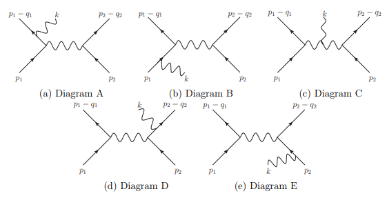
Figure 2.2: Feynman diagrams that contribute to the 5-point radiation amplitude in SQED. Figure adapted from [6]

Let us however take an alternative road which uses what we have learned from the computation of the leading order impulse in the previous example. That is, in the classical limit, the amplitude can be obtained from the unitarity gluing of lower multiplicity amplitudes. This is nothing but the well known fact that up to contact terms (although in some cases they are not present), the scattering amplitudes can be reconstructed from unitary cuts, where the internal particles become on-shell, and the amplitude factorizes into the product of two on-shell amplitudes [171].

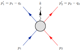
Figure 2.3: Bremsstrahlung radiation (outgoing photon) emitted during the scattering of two massive charge particles thought the exchanging electromagnetic waves.

For the case of $M_{4}$, at leading order we in the PL (PM) expansion, the classical piece of the amplitude can then be computed from the formula

$$\boxed{\langle M_{4}^{h}\rangle=\frac{n_{h}}{q^{2}}}\,,$$ (2.40)

where $n_{h}$ is a local numerator. This form of the 4-point amplitude is general, and works for the electromagnetic and gravitational theory, including spin effects as we will see in chapter 4. For the case of the classical 4-point amplitude at leading PL order, we can identify the scalar numerator by caparison to (2.26). $n_{\text{ph}}=4e^{2}Q_{1}Q_{2}\,p_{1}{\cdot}p_{2}$

For the case of the five point amplitude, the relevant factorization channel that encapsulate the classical contribution, are those for which the amplitudes factorizes into the product of our favorite 3-point (2.4) and the scalar Compton amplitude (2.5), as follows

(2.41)

that is, the channels for which $q_{1}^{2}=0$ and $q_{2}^{2}=0$. We stress this factorization enclose the classical contribution even in the presence of spin as we will see in chapter 4.

Let us now see how this factorization allow us to recover the Bremshrtralugh radiation formula for scalar objects. At the first factorization channel, $q_{2}^{2}=0$, the residues can be computed via

$$\text{Res}M_{5}^{\text{SQED}}\Big{|}_{q_{2}^{2}=0}=\Big{(}A_{4}^{\text{L}\,,\mu}\,\eta_{\mu\nu}\,A_{3}^{\text{R}\,,\nu}\Big{)}\Big{|}_{q_{2}^{2}=0}$$ (2.42)

where

$$A_{3}^{\text{R}\,,\nu} =2eQ_{2}\,p_{2}^{\nu}\,,$$ (2.43)

$$A_{4}^{\text{L}\,,\mu} =\frac{2e^{2}Q_{1}^{2}}{(p_{1}{\cdot}k)(p_{1}{\cdot}q_{2})}(p_{1}{\cdot}q_{2}\,F^{\mu\alpha}p_{1\alpha}-p_{1}^{\mu}q_{2}{\cdot}F{\cdot}p_{1})\Big{|}_{q_{2}^{2}=0}\,.$$ (2.44)

Now, the on-shell condition for the outgoing massive particles imply $p_{1}{\cdot}q_{1}=q_{1}^{2}/2$ and $p_{2}{\cdot}q_{2}=q_{2}^{2}/2$. This shows that, although the products $p_{i}{\cdot}q_{i}$ naively scale as $\sim\hbar$, they in fact scale as $\sim\hbar^{2}$ and are therefore subleading in the classical limit. Notice also that momentum conservation dictates $p_{1}{\cdot}q_{2}=p_{1}{\cdot}k-q_{1}^{2}/2$, where the second factor can be dropped in the classical limit The analog result follows for the factorization channel $q_{1}^{2}=0$.

We have learned then that in the classical limit, the Bremsstrahlung amplitude has the following form:

$$\boxed{\langle M_{5}^{h}\rangle{=}\frac{1}{(q{\cdot}k)^{h-1}}\left[\frac{n_{h}^{(a)}}{(q^{2}{-}q{\cdot}k)(p_{1}{\cdot}k)^{2}}+(-1)^{h+1}\frac{n_{h}^{(b)}}{(q^{2}{+}q{\cdot}k)(p_{2}{\cdot}k)^{2}}\right]}\,,$$ (2.45)

where we have further write the momentum transfer $q_{i}$ in the symmetric variable $q$ via $q=\frac{q_{1}-q_{2}}{2}$. Here we have written $h=1,2$ to denote the photon and graviton emission, since, as we will argue in chapter 4 and chapter 6, this formula also holds for gravity, even in the presence of spin. For the time being we can just set $h=1$ as it is the case we are here interested in.

The scalar numerators for photons emission, can be rearrange in the form

$$n_{0,\rm{ph}}^{(a)}{=}4e^{3}Q_{1}^{2}Q_{2}p_{1}{\cdot}R_{3}{\cdot}F{\cdot}p_{1},\quad n_{0,\rm{ph}}^{(b)}{=}4e^{3}Q_{1}Q_{2}^{2}p_{3}{\cdot}R_{1}{\cdot}F{\cdot}p_{3},$$ (2.46)

where we have introduced the notation $R_{i}^{\mu\nu}{=}p_{i}^{[\mu}(\eta_{i}2q{-}k)^{\nu]}$, with $\eta_{1}=1$ and $\eta_{2}=-1$. We have to keep in mind this numerators are valid on the support of the on-shell condition for the outgoing massive particles.

To be more precise, we can now write the radiated photon field for the scattering of two scalar charged particles in SQED, as given by our KMOC formula (1.16) as follows

$$A^{\mu}(k)=ie^{k{\cdot}\tilde{b}}\int\hat{d}^{D}q\prod_{i=1}^{2}\hat{\delta}(2p_{i}{\cdot}q)e^{-iq{\cdot}b}\left[\frac{n_{0,\text{ph}}^{(a)}}{(q^{2}{-}q{\cdot}k)(p_{1}{\cdot}k)^{2}}+\frac{n_{0,\text{ph}}^{(b)}}{(q^{2}{+}q{\cdot}k)(p_{2}{\cdot}k)^{2}}\right]\,,$$ (2.47)

where we have use $\tilde{b}=\frac{1}{2}(b_{1}+b_{2})$, and we have defined the impact parameter $b=b_{2}-b_{1}$. One can show this formula recovers the classical result of Goldberger and Ridgway [80] for colourless charges, upon the change of variables $l_{1}=q+k/2$ and $l_{2}=-q+k/2$, and set $b_{2}=0$.

Photon exponential soft theorem

We will not evaluate explicitly integral (2.47) here, but will study a very interesting feature that arise if the photon emission is soft , namely, the soft exponentiation of the scalar classical 5-point amplitude. This will also be a feature for the gravitational case as we will show in chapter 4. For this we make use of the exponential form of the Compton amplitude (2.23) to read exponential form of numerators entering in the 5-point amplitude (2.45). This is, the numerators $n_{0,\text{ph}}^{(a)}$ can be read off directly from (2.23) as follows: Replacing $\epsilon_{1}$ by $p_{2}$, powers of the orbit multipole $F_{\epsilon}$ translate to powers of $F_{p}{=}p_{1}{\cdot}F{\cdot}p_{2}$, whereas $F_{k}$ now becomes $F_{iq}{=}\eta_{i}(p_{i}{\cdot}F{\cdot}q)$, with $\eta_{1}{=}{-}1,\eta_{2}=1$. The soft expansion (2.23) with respect to $k_{2}=k$ becomes

$$n_{0,\text{ph}}^{(a)}=F_{1q}\,e\,Q_{1}\,e^{-\frac{F_{p}}{F_{1q}}(p_{1}{\cdot}k)\frac{\partial}{\partial(p_{1}{\cdot}p_{3})}}\left[4e^{2}Q_{1}\,Q_{2}p_{1}{\cdot}p_{2}\right].$$ (2.48)

Further writing $\frac{1}{q^{2}\pm q\cdot k}=e^{\pm q\cdot k\frac{\partial}{\partial q^{2}}}\frac{1}{q^{2}}$ turns (2.45) into

$$\boxed{\langle M_{5}^{\rm SQED}\rangle=\sum_{i=1,2}\mathcal{S^{\text{SQED}}}_{i}e^{\eta_{i}\left(F_{p}\frac{p_{i}{\cdot}k}{F_{iq}}\frac{\partial}{\partial(p_{1}{\cdot}p_{3})}+q{\cdot}k\frac{\partial}{\partial q^{2}}\right)}\langle M_{4}^{\rm SQED}\rangle\,}$$ (2.49)

where is given in (2.26). We have defined $\mathcal{S^{\text{SQED}}}_{i}{=}eQ_{i}\frac{F_{iq}}{(p_{i}{\cdot}k)^{2}}$ . This expression can be used to obtain $\langle M^{\rm SQED}_{5}\rangle$ from $\langle M_{4}^{\rm SQED}\rangle$ as an expansion in the photon momentum $k^{\mu}$ to any desired order in the soft expansion (sub-subleading orders were studied in [172, 173, 174]).

One can check explicitly that $\mathcal{S}_{1}+\mathcal{S}_{2}$ corresponds to the $\hbar\to 0$ limit of the Weinberg Soft Factor for the full $M_{5}$ [175]. The first order of the exponential analogously corresponds to the $\hbar\to 0$ limit of the subleading soft factor of Low [167, 176].

Let us focus for simplicity on the leading order of (2.49). As we will see in chapter 5, for bounded orbits $\omega\sim\frac{v}{r}$ the wave frequency expansion becomes a non-relativistic expansion [31], where the Maxwell dipole emission formula (an analogously the Einstein quadrupole formula) can be derived from the Weinberg soft theorem. For classical scattering we can use the leading soft term to obtain the Memory Effect as $R{\to}\infty$. Plugging (2.49) into (2.47) we get

$$\int\frac{d^{D}q}{(2\pi)^{D-2}}\delta(2q\cdot p_{1})\delta(2q\cdot p_{2})e^{iq\cdot b}\left(\sum_{i=1,2}\mathcal{S}_{i}\right)\langle M_{4}^{{\rm SQED}}\rangle$$

as $k\to 0$. Evaluating the sum and using (2.27) as a definition of the linear impulse $\Delta p_{1}=-\Delta p_{2}$ we obtain

$$\epsilon_{\mu}A^{\mu}=\frac{1}{p_{1}{\cdot}k\,p_{2}{\cdot}k}\left(\frac{e\,Q_{1}\,p_{1}}{p_{1}{\cdot}k}{+}\frac{e\,Q_{2}\,p_{2}}{p_{2}{\cdot}k}\right){\cdot}F{\cdot}\Delta p{+}\mathcal{O}(k^{0}),$$ (2.50)

which at leading order in $\Delta p$ (or $e$) becomes

$$A^{\mu}(k)=\Delta\left[\frac{e\,Q_{1}\,p_{1}^{\mu}}{p_{1}{\cdot}k}+\frac{e\,Q_{2}\,p_{2}^{\mu}}{p_{2}{\cdot}k}\right]\,.$$ (2.51)

This is nothing but the classical leading soft factor for two incoming and two outgoing massive particles [177]

$$A_{\mu}^{\omega^{-1}}(\hat{n})\,=\,\sum_{i=1}^{N_{in}}\,Q_{i}\,\frac{1}{p_{i}\cdot n}\,p_{i}^{\mu}\,-\,\sum_{i=1}^{N_{out}}\,Q_{i}\,\frac{1}{p_{i}\cdot n}\,p_{i}^{\mu}\,,$$ (2.52)

once we write the outgoing momenta as a perturbative expansion in powers of the impulse acquired by the massive particles order by order in perturbation theory

$$p_{i\,\text{out}}^{\mu}\,=\,p_{i\,\text{in}}^{\mu}+\sum_{L=0}\,e^{2(L+1)}\,(\triangle p^{(L)})_{i}^{\mu}\,,$$ (2.53)

and take the leading order in the coupling $e$ (i.e. $L=0$). We have then connected non-perturbative results for classical soft theorems to the perturbative scattering amplitude approach to the computation of classical radiation. In general, we will show in chapter 3 that classical soft theorems impose and infinite tower of constraints on KMOC computations, where the tower arises from the loop expansion of the outgoing momenta (2.53).

As last comment, it is well known that the leading and subleading soft theorems QED are universal, independent of the details of the computation, as well as the matter content [178, 172, 173, 179, 177]. In this section we have reproduced the leading soft theorem starting from the scattering of scalar charge particles only. This means adding intrinsic structure to the particle such as spin, should not change the result (2.52) for the radiated photon field. This, as we will see in chapter 4, is a consequence of the spin universality of $A_{3}$ and $A_{4}$ amplitude, which is inherited by the two-body radiative amplitude $M_{5}$.

2.4 2PL linear impulse in SQED

In the final part of this chapter we do the explicit evaluation of the 2PL linear impulse integral for scalars particles. This integral was derived using the KMOC formalism in the original paper by the authors [78], whose final result was left implicit, and can be obtained directly from the Feynman diagrams 1-loop diagrams in SQED. We will use integration techniques outlined in section 2.3 to show the final result agrees with the classical computation of Saketh et al [76].

As shown by the authors [78], the classical impulse receives contribution from only of the triangle, boxes and cross-box diagrams 1-Loop diagrams. After carefully taken the classical limit of each contribution as described in section 1.2, the authors show superclassical fragments cancel between the linear and quadratic in amplitude contributions to the linear impulse (1.12). As for the classical contribution, the authors arrive at the following integral:

$$\Delta p^{(1)\,\mu}_{1}=\frac{i}{4}\int\hat{d}^{4}q\prod_{i}\hat{\delta}(p_{i}{\cdot}q)e^{-ib{\cdot}q}\left[\mathcal{I}_{1}^{\mu}+\mathcal{I}_{2}^{\mu}+\mathcal{I}_{3}^{\mu}\right],$$ (2.54)

where the $\mathcal{I}_{i}^{\mu}$ integrals resemble the contributions to the 4 point amplitude from the different Feynman diagrams. The firs one comes from the contribution from the triangle diagrams

$$\mathcal{I}_{1}^{\mu}=2e^{4}\left(Q_{1}Q_{2}\right)^{2}q^{\mu}\sum_{i}\int\hat{d}^{4}l\frac{m_{i}^{2}\hat{\delta}(p_{i}{\cdot}l)}{l^{2}(l-q)^{2}}\,.$$ (2.55)

Next we have the contribution coming from the Boxes, which once by canceling the term $Z$ in $(\ref{eq:4pt 1L classical explicit})$, using the cut-Box diagram, reads

$$\mathcal{I}_{2}^{\mu}=2e^{4}\left(Q_{1}Q_{2}p_{1}{\cdot}p_{2}\right)^{2}q^{\mu}\sum_{i,j\,i\neq j}\int\hat{d}^{4}l\frac{l{\cdot}(l-q)}{l^{2}(l-q)^{2}}\frac{\hat{\delta}(p_{j}{\cdot}l)}{(p_{i}{\cdot}l+i\epsilon)^{2}},$$ (2.56)

Finally, we have the 4 point cut-box contribution

$$\mathcal{I}_{3}^{\mu}=-2ie^{4}\left(Q_{1}Q_{2}p_{1}{\cdot}p_{2}\right)^{2}\int\hat{d}^{4}l\frac{l{\cdot}(l-q)l^{\mu}}{l^{2}(l-q)^{2}}\left[\hat{\delta}^{\prime}(p_{1}{\cdot}l)\hat{\delta}(p_{2}{\cdot}l)-\hat{\delta}(p_{1}{\cdot}l)\hat{\delta}^{\prime}(p_{2}{\cdot}l)\right].$$ (2.57)

Let us start with the computation of the triangle diagrams which corresponds to the first term in (2.54). Using (2.55), we have

$$\tilde{\mathcal{I}}_{1}^{\mu}=\frac{ie^{4}}{2}(Q_{1}Q_{2})^{2}\int\hat{d}^{4}q\hat{d}^{4}l\hat{\delta}(p_{1}{\cdot}q)\hat{\delta}(p_{2}{\cdot}q)\frac{q^{\mu}}{l^{2}(l-q)^{2}}e^{-iq{\cdot}b}\left[m_{1}^{2}\hat{\delta}(p_{1}{\cdot}l)+m_{2}^{2}\hat{\delta}(p_{2}{\cdot}l)\right]\,.$$ (2.58)

We can do the integral in $l^{0}$ by going to the rest frame of particle $1$ (or $2$) then getting $\hat{\delta}(l^{0})$ as the zero energy condition. Notice that we can also set $q^{0}=0$ by using one of the on-shell delta functions in $q$. With this in mind the previous integral takes the form

$$\tilde{\mathcal{I}}_{1}^{\mu}=\frac{ie^{4}}{2}(Q_{1}Q_{2})^{2}(m_{1}+m_{2})\int\hat{d}^{4}q\hat{d}^{3}\vec{l}\hat{\delta}(p_{1}{\cdot}q)\hat{\delta}(p_{2}{\cdot}q)\frac{q^{\mu}}{\vec{l}^{2}(\vec{l}-\vec{q})^{2}}e^{-iq{\cdot}b}\,.$$ (2.59)

The integral in $\hat{d}^{3}\vec{l}$ is easy to evaluate using Schwinger parameters, see for instance eq. $(7.9)$ in [46] . Using those results we get

$$\tilde{\mathcal{I}}_{1}^{\mu}=\frac{ie^{4}}{16\sqrt{D}}(Q_{1}Q_{2})^{2}(m_{1}+m_{2})\int\hat{d}^{2}q_{\perp}\frac{q_{\perp}^{\mu}}{q_{\perp}}e^{-iq_{\perp}{\cdot}b},$$ (2.60)

where we have further evaluated two of the $\hat{d}^{4}q$ integrals using the expansions for the momenta (3.3). Evaluation of the remaining integral can be done in polar coordinates, upon trading $q_{\perp}^{\mu}$ in the numerators by a derivative w.r.t. the impact parameter. The final answer will be

$$\tilde{\mathcal{I}}_{1}^{\mu}=-\frac{e^{4}}{32\pi}(m_{1}+m_{2})\frac{(Q_{1}Q_{2})^{2}}{\sqrt{D}}\frac{b^{\mu}}{|b|^{3}}.$$ (2.61)

Next we move to the evaluation of the last term in (2.54) using (2.57),

$$\tilde{\mathcal{I}}_{3}^{\mu}=\frac{e^{4}}{2}(Q_{1}Q_{2}p_{q}{\cdot}p_{2})^{2}\int\hat{d}^{4}q\hat{d}^{4}l\hat{\delta}(p_{1}{\cdot}q)\hat{\delta}(p_{2}{\cdot}q)\frac{l{\cdot}(l{-}q)}{l^{2}(l{-}q)^{2}}l^{\mu}e^{-iq{\cdot}b}[\hat{\delta}^{\prime}(p_{1}{\cdot}l)\hat{\delta}(p_{2}{\cdot}l){-}\hat{\delta}(p_{1}{\cdot}l)\hat{\delta}^{\prime}(p_{2}{\cdot}l)],$$ (2.62)

where the tilde over $\mathcal{I}_{3}$ indicates inclusion of the $q$ integration. To evaluate this integral we can expand the momentum $l$ in an analogous way to the $q$ momentum in (2.30 - 2.31), with say $\alpha_{i}\to\beta_{i}$, and $x_{i}\to y_{i}=p_{i}\cdot l$. The resulting integrand takes the form (2.33), and therefore we can evaluate the time and longitudinal components using integrating by parts one time (2.34). That is, we can write

$$\tilde{\mathcal{I}}_{3}^{\mu}=\frac{1}{\sqrt{\mathcal{D}}}\int\hat{d}^{4}q\hat{\delta}(p_{1}{\cdot}q)\hat{\delta}(p_{2}{\cdot}q)\hat{d}^{2}l_{\perp}\hat{d}y_{1}\hat{d}y_{2}e^{-iq{\cdot}b}\left[\hat{\delta}^{(1)}(y_{1})\hat{\delta}^{(0)}(y_{2})-\hat{\delta}^{(0)}(y_{1})\hat{\delta}^{(1)}(y_{2})\right]f_{u}^{\alpha}(y_{1},y_{2},l_{\perp},\sigma),$$ (2.63)

with the identification of the integrand function

$$f_{u}^{\alpha}(y_{1},y_{2},l_{\perp},\sigma)=\frac{e^{4}}{2}\left(Q_{1}Q_{2}p_{1}{\cdot}p_{2}\right)^{2}\frac{(\beta_{2}p_{1}{+}\beta_{1}p_{2}+l_{\perp})^{\alpha}\left((\beta_{2}p_{1}{+}\beta_{1}p_{2})^{2}{+}l_{\perp}^{2}{-}l_{\perp}{\cdot}q_{\perp}\right)}{\left((\beta_{2}p_{1}{+}\beta_{1}p_{2})^{2}{+}l_{\perp}^{2}\right)\left((\beta_{2}p_{1}{+}\beta_{1}p_{2})^{2}{+}(l_{\perp}{-}q_{\perp})^{2}\right)}\,.$$

where in addition to the $l$-expansion, we have used the expansion for the $q$-momentum (2.30), and set $x_{i}\to 0$ using the support of the delta functions $\hat{\delta}(p_{i}{\cdot}q)$ . Next, to use (2.34) after integration by parts we need to evaluate the derivatives of the form

$$\frac{\partial}{\partial y_{i}}f_{u,ij}^{\alpha}\Bigg{|}_{y_{i}=y_{j}=0}=\frac{4e^{4}}{\mathcal{D}}\left(Q_{i}Q_{j}p_{i}{\cdot}p_{j}\right)^{2}p_{j,\beta}p_{j}^{[\beta}p_{i}^{\alpha]}\frac{l_{\perp}{\cdot}(l_{\perp}-q_{\perp})}{l_{\perp}^{2}(l_{\perp}-q_{\perp})^{2}}\,,$$ (2.64)

With all the tools at hand, it is then direct to show that the integral (2.63) simplifies to

$$\tilde{\mathcal{I}}_{3}^{\mu}=-e^{4}\frac{\left(Q_{1}Q_{2}p_{1}{\cdot}p_{2}\right)^{2}}{\mathcal{D}^{2}}\left[p_{2,\beta}p_{2}^{[\beta}p_{1}^{\alpha]}{-}p_{1,\beta}p_{1}^{[\beta}p_{2}^{\alpha]}\right]\int\hat{d}^{2}q_{\perp}\hat{d}^{2}l_{\perp}e^{-ib{\cdot}q_{\perp}}\frac{l_{\perp}{\cdot}(l_{\perp}{-}q_{\perp})}{l_{\perp}^{2}(l_{\perp}{-}q_{\perp})^{2}}.$$ (2.65)

Next we do the usual change of variables $q_{\perp}=\bar{q}_{\perp}+l_{\perp},$ so that

$$\tilde{\mathcal{I}}_{3}^{\mu}=-\frac{e^{4}}{\mathcal{D}}\left[p_{2,\beta}p_{2}^{[\beta}p_{1}^{\alpha]}{-}p_{1,\beta}p_{1}^{[\beta}p_{2}^{\alpha]}\right]\left[\frac{Q_{1}Q_{2}p_{1}{\cdot}p_{2}}{\sqrt{\mathcal{D}}}\int\hat{d}^{2}q_{\perp}\hat{d}^{2}l_{\perp}e^{-ib{\cdot}q_{\perp}}i\frac{\bar{q}_{\perp}}{\bar{q}_{\perp}^{2}}\right]^{2}.$$ (2.66)

in the big bracket we recognize the Leading order impulse $(\ref{eq:LO_impulse_interm})$, which in turn allow write the final result as

$$\tilde{\mathcal{I}}_{3}^{\mu}=e^{4}\frac{(Q_{1}Q_{2}p_{1}{\cdot}p_{2})^{2}}{8\pi^{2}\mathcal{D}^{2}|b|^{2}}\left[\left(m_{1}^{2}+p_{1}{\cdot}p_{2}\right)p_{2}^{\mu}-\left(m_{2}^{2}+p_{1}{\cdot}p_{2}\right)p_{1}^{\mu}\right].$$ (2.67)

The final task the evaluation of the e box and cross-box diagrams from integral (2.56). We now show they provide vanishing contribution in the conservative sector. We can see this by first dropping the term proportional to $l\cdot l$ in the numerator of (2.56) since it give rise to non local contributions. Next, using the same philosophy of [39], we can write $2l\cdot q=l^{2}+q^{2}-(l-q)^{2}$, and discarding again non local contributions; the integral (2.56) becomes

$$\mathcal{I}_{2}^{\mu}=-e^{4}\left(Q_{1}Q_{2}p_{1}{\cdot}p_{2}\right)^{2}q^{\mu}\sum_{i,j\,i\neq j}q^{2}\int\hat{d}^{4}l\frac{\hat{\delta}(p_{j}{\cdot}l)}{l^{2}(l-q)^{2}(p_{i}{\cdot}l+i\epsilon)^{2}},$$ (2.68)

using the fact that at NLO no net four-momentum is radiated, radiation poles do not contribute to the integral, we can choose a contour in the opposite half of the plane were (2.56) has the double poles $(p{\cdot}l+i\epsilon)^{2}$, and then getting a vanishing integral. Indeed this was also done for the gravitational case in [38] eq. (4.26). In conclusion, the NLO electro-magnetic impulse is the sum of (2.61) and (2.67),

$$\Delta p_{1}^{(1)\,\mu}=\tilde{\mathcal{I}}_{1}^{\mu}+\tilde{\mathcal{I}}_{3}^{\mu}=-\frac{e^{4}}{32\pi^{2}|b|^{3}}\frac{(Q_{1}Q_{2})^{2}}{\mathcal{D}}\left[\pi\sqrt{\mathcal{D}}(m_{1}+m_{2})b^{\mu}+4\frac{(p_{1}{\cdot}p_{2})^{2}(p_{1}{+}p_{2})^{2}|b|}{\mathcal{D}}p^{\mu}\right]\,,$$ (2.69)

where we have introduced the center of mass momentum $p^{\mu}$ via

$$p^{\mu}=\frac{m_{1}m_{2}}{(p_{1}+p_{2})^{2}}\left[\left(\frac{m_{2}}{m_{1}}+\frac{p_{1}\cdot p_{2}}{m_{1}m_{2}}\right)p_{1}^{\mu}-\left(\frac{m_{1}}{m_{2}}+\frac{p_{1}\cdot p_{2}}{m_{1}m_{2}}\right)p_{2}^{\mu}\right]\,,$$ (2.70)

and therefore recovering the classical result of Saketh et al [76].

2.5 Outlook of the chapter

In this chapter we have introduced some of the main ideas in the computation of classical observables directly from the classical limit of scattering amplitudes, in company of the KMOC formalism. In particular, we have focused in interactive, structure-less compact charge objects, both, tree, and 1-loop level. We have seen how the main ingredients $A_{n}$, $n=3.4$, in the computation of two body amplitudes $M_{m}$, $m=4,5$, have very interesting properties that are inherited by the latter. In addition, we have seen how soft theorems play a crucial role in the computation of low energy bremhstralugh radiation. In chapter 3, we will continue exploring some interesting properties regarding the computation of classical soft radiation in SQED to higher orders in perturbation theory. In chapter 5 we will show how soft theorems are actually also important in the computation of radiation for bounded orbit scenarios, where the soft expansion is closely connected to the source multipole moment expansion.

Many of the tools learned in this chapter will be of used in the remaining ones, specially when we discuss interacting spinning massive matter, and the covariant spin multipole double copy in chapter 4. The discussion regarding the Thomson scattering will be generalized for the scattering of waves off spinning black holes in chapter 7.

Chapter 3 Soft constraints on KMOC for electromagnetic radiation

3.1 Introduction

In chapter 2 we have started the study of classical radiation directly from the classical limit of QFT scattering amplitudes through the KMOC formalism. In particular, we have seen that the radiated photon field in a classical $2\to 3$ scattering process, at leading order in the frequency expansion of the emitted wave, is entirely capture by the classical limit of the so called Weinberg soft theorem [175]. In this chapter we extend the discussion of classical soft theorems, and in particular, we will discuss the implication they have on the computation of classical soft radiation directly from perturbative amplitudes, to all orders in perturbation theory. We will show that to a given order in perturbation theory, the classical leading soft photon theorem impose an infinite tower of constraints on the expectation value of the product of monomials of exchange momenta in the KMOC formula for radiation (1.15).

Before going into the main computation, let us in the remaining of this section, review some facts about classical soft theorems and summarize the main results of this chapter. This chapter is mostly based on previous work by the author [106].

Facts from classical soft theorems and summary of the results of the chapter

Classical soft photon (graviton) theorems [178, 172, 173, 179, 177] are exact statements about soft radiation emitted during a generic electro-magnetic (gravitational) scattering process. As shown in the seminal works by Sahoo and Sen[173], Saha, Sahoo and Sen [177], and Sahoo [180], in four dimensions if we expand the electro-magnetic (or gravitational) radiative field in the frequency of the emitted radiation, then the following terms in the expansion have a universal analytic form independent of the details of the scattering dynamics or even spins of the scattering particles

$$A_{\mu}(\omega,\hat{n})\,=\,\frac{1}{\omega}\,A_{\mu}^{\omega^{-1}}(\hat{n})\,+\,\sum_{I=1}^{2}\,\omega^{I}(\ln\omega)^{I+1}\,A_{\mu}^{\ln^{I+1}}(\hat{n})\,+\,\cdots\,.$$ (3.1)

Here $\hat{n}$ is a unit vector pointing towards the direction of observation, and $\cdots$ indicate sub-sub-leading terms in the soft expansion. It was conjectured in [180] that even among the subⁿ-leading terms the coefficients of $\omega^{n}\,\ln^{n+1}\omega\ ,n\,\geq\,3$ are universal while other terms in the soft expansion are non-universal and depend on the details of the dynamics. In [181], first such non-universal soft factor proportional to $\omega\ln\omega$ was computed and was shown to depend on the spin of the scattering particles.

Each coefficient in the above expansion is a function of incoming and outgoing momenta and charges of the scattering particles. For example, the leading coefficient $A_{\mu}^{\omega^{-1}}(\hat{n})$ is simply the Weinberg soft photon factor (2.52), which we reintroduce here for the reader’s convenience

$$A_{\mu}^{\omega^{-1}}(\hat{n})\,=\,\sum_{i=1}^{N_{in}}\,Q_{i}\,\frac{1}{p_{i}\cdot n}\,p_{i}^{\mu}\,-\,\sum_{i=1}^{N_{out}}\,Q_{i}\,\frac{1}{p_{i}\cdot n}\,p_{i}^{\mu}\,.$$ (3.2)

Here $\{(Q_{1},p_{1}),\,\cdots,\,(Q_{i},p_{i})\,\}$ is the collection of the charges and momenta of scattering particles, and $n^{\mu}\,=\,(1,\hat{n})$. Although the exact expressions for sub-leading and higher order log soft factors in eqn.(3.1) are more complicated, they are all functions of asymptotic data, namely charges and momenta of scattering particles, which we do not show here explicitly. The form of (3.2) can be obtained by computing the early and late time electromagnetic waveform emitted during the scattering of the charged particles involved. The computation requires then to solve the classical EoM for all of the particles involved, obtaining $x_{a}(\sigma_{\pm})$, with $\sigma_{p}m$ the incoming/outgoing particles proper time. Having these solutions at hand, we can then compute a electromagnetic current of the form $j^{\mu}(x)\sim\sum_{a}\int d\sigma\delta^{4}(x-x_{a}(\sigma))\frac{dx_{a}}{d\sigma}$, which enters as a source for electromagnetic waves, as given by (1.18), whose LO behaviour in the low energy expansion result into (3.2). For a detail computation see Section 4.1 in [177]. The key observation is this probe assumes all particles momenta to be independent one from another, and in this regard, the solution is valid to all orders in perturbation theory.

From the perspective of scattering dynamics, these theorems are rather non-trivial as they are non perturbative in the coupling ans we just mentioned. If we consider a class of scattering processes which can be analysed perturbatively (such as large impact parameter scattering, as we have seen in previous section, with $N_{in}=N_{out}=N$) then every outgoing momenta admits the perturbative expansion (2.53), in terms of the incoming momenta

$$p_{i\,+}^{\mu}\,=\,p_{i\,-}^{\mu}+\sum_{L=0}\,e^{2(L+1)}\,(\triangle p^{(L)})_{i}^{\mu}\,,$$ (3.3)

where $e$ is the coupling constant, and $(\triangle p^{(L)})^{\mu}$ is the linear impulse evaluated at $L$-th order in the perturbation theory ($L=0$ being the LO impulse which we explored in previous chapter). This expansion is just a fact that in a large impact parameter scattering process, particles’ outgoing momenta are determined by the incoming momenta plus the equations of motion governing the dynamics of the system. We thus see when expanded in the coupling, the Weinberg soft photon factor has a rather intricate structure

$$A_{\mu}^{\omega^{-1}}(\hat{n})\,=\,\sum_{s=1}^{N}\,e\,Q_{s}\sum_{n=0}e^{2(n+1)}\,\sum_{i=0}^{n}\,V^{\mu}_{s\,\alpha_{1}\,{\cdots}\,\alpha_{i+1}}\ \smashoperator[]{\sum_{\begin{subarray}{c}L_{1}+\,\cdots+\,L_{i+1}=0\\ (L_{1}+L_{i+1})+(i+1)\,=n\end{subarray}}^{n+1-i}}\ (\,(\triangle p^{(L_{1})})^{\alpha_{1}}\,{\cdots}\,(\triangle p^{(L_{i+1})})^{\alpha_{i+1}}\,)\,,$$ (3.4)

where the sum $\sum_{L_{1},\,\cdots,\,L_{i+1}=0\,|\,(L_{1}+L_{i+1})+(i+1)\,=n}^{n+1-i}$ is over products of impulses at $L_{1},\,\cdots,\,L_{i+1}$ orders in the coupling respectively. In the above equation we have defined the tensors

$$V^{\mu}_{s\,\alpha_{1}\,\cdots\,\alpha_{i+1}}\,=\,{\color[rgb]{0,0,0}(-1)^{i}}\,\Big{[}\,\frac{(i+1)\,!\,}{(p_{s}\cdot k)^{i+1}}\delta^{\mu}_{(\alpha_{1}}\,k_{\alpha_{2}}\,\cdots\,k_{\alpha_{i+1})}\,-\,\frac{1}{(p_{s}\cdot k)^{i+2}}\,p_{s}^{\mu}\,k_{\alpha_{1}}\,\cdots\,k_{\alpha_{i+1}}\,\Big{]}\,,$$ (3.5)

which are the remainders from doing the perturbative expansion of Weinberg soft factor.

Classical Soft photon (or graviton) theorem are independent of the details of the hard scattering and are applicable to perturbative scattering at finite impact parameter as well as collisions. However, to prove the classical soft theorems via perturbative analysis (even in the case where hard scattering can be treated perturbatively) is a highly non-trivial task as one has to resum the perturbation series. But the discussion above demonstrates that, due to their universality, classical soft theorems can serve as powerful tool for any method which computes electro-magnetic (or gravitational) radiation using (perturbative) scattering amplitudes. For one, it can serve as a strong diagnostic for the perturbative results of radiation kernel and when used in conjunction with the perturbative results (such as analytic expressions for impulse in the PL and PM expansions), it can produce interesting insights such as providing analytical formulae for classical radiation in terms of incoming kinematic data order by order in perturbation theory, an example of which we saw in previous section in the discussion around (2.51)

One such methods aforementioned, was developed by KMOC [78], as it is now familiar for us from section 1.2, which allows to compute classical electromagnetic (gravitational) observables from the classical limit of quantum scattering amplitudes, as exemplified in previous chapter. In this chapter we initiate a study of the implications of classical soft theorems for KMOC formalism. As we will show, consistency with the leading classical soft theorem imposes an infinite hierarchy of constraints on KMOC observables. In order to state these constraints we introduce following conventions.

The scattering process we consider is a $2\,\rightarrow\,2$ scattering process in which two incoming charged particles with momenta $p_{1},p_{2}$ and charges $Q_{1},\,Q_{2}$ scatter via electro-magnetic interactions as well as any other higher derivative interaction which is long range such that the KMOC formalism applies to this scattering. As the classical soft theorems are universal and independent of the details of the scattering, classical limit of the radiation kernel should generate the soft factors for any perturbative amplitude involving charged particles in the external states and a photon.

To each of the two massive particles we can associate certain classical observables defined as follows:
(1) Let $V^{\mu}_{\alpha_{1}\,\cdots\,\alpha_{i}}$ be the projection operator (3.5), associated to particle $1$, that is

$$V^{\mu}_{\alpha_{1}\,\cdots\,\alpha_{i}}\,=\,(-1)^{i+1}\,\Big{[}\,\frac{i!}{(p_{1}\cdot k)^{i}}\,\delta^{\mu}_{(\alpha_{1}}\,k_{\alpha_{2}}\,\cdots\,k_{\alpha_{i})}\,-\frac{1}{(p_{1}\cdot k)^{i+1}}\,p_{1}^{\mu}\,k_{\alpha_{1}}\,\cdots\,k_{\alpha_{i}}\,\Big{]}\,.$$ (3.6)

(2) Now consider certain moments of the exchange momenta

$$\begin{array}[]{lll}{\cal T}^{(n)\,\alpha_{1}\,\cdots\,\alpha_{i}}\,:=\,\hbar^{\frac{3}{2}}\Big{[}i\int\,\hat{d}\mu_{q}\,q^{\alpha_{1}}\,\cdots\,q^{\alpha_{i}}\,e^{-iq{\cdot}b}\,M^{(n)}(p_{1},p_{2}\,\rightarrow\,p_{1}-q,p_{2}+q)\\ \hskip 99.58464pt+\,\sum_{X=0}^{n-1}\,\int\,\prod_{m=0}^{X}d\Phi(r_{m})\,\hat{d}\mu_{q}\,\hat{d}\mu_{w,X}w^{\alpha_{1}}\,\cdots\,w^{\alpha_{i}}\,e^{-iq{\cdot}b}\\ \hskip 128.0374pt\times\sum_{a_{1}=0}^{n-1-X}M^{(a_{1})}(p_{1},p_{2}\,\rightarrow\,p_{1}-w,p_{2}+w,\,r_{X})\\ \hskip 128.0374pt\times M^{(n-a_{1}-X-1)\star}(p_{1}-w,p_{2}+w,\,r_{X}\,\rightarrow\,p_{1}-q,p_{2}+q)\Big{]}\,\,,\end{array}$$ (3.11)

where $b$ is the impact parameter in the $2\to 2$ scattering process. In the above equation we have introduced the following notations which will be used throughout this chapter.

• $M^{(a)}(p_{1}^{i},\,p_{2}^{i}\,\rightarrow\,p_{1}^{f},p_{2}^{f})$ is the (stripped) amplitude for a 4 point scattering at $a$-th order in perturbation theory, and analogously for the other amplitudes with additional momentum labels.

• The integral measure $\hat{d}\mu_{q}$ is defined via

  $$\hat{d}\mu_{q}=\hat{d}^{4}q\hat{\delta}(2p_{1}{\cdot}q-q^{2})\hat{\delta}(2p_{2}{\cdot}q+q^{2}),$$ (3.12)

  where $\hat{d}^{4}q=\frac{d^{4}q}{(2\pi)^{4}}$, and the hat on $\delta$-fn. indicates it is defined as

  $$\hat{\delta}(x)\,=\,-i\,[\,\frac{1}{x-i\epsilon}\,-\frac{1}{x+i\epsilon}\,]\,,$$ (3.13)

  and analogous for $\hat{d}\mu_{w,X}$,

  $$\hat{d}\mu_{w,X}=\hat{d}^{4}q\hat{\delta}(2p_{1}{\cdot}w-w^{2})\hat{\delta}(2p_{2}{\cdot}(w+r_{X})+(w+r_{X})^{2})$$ (3.14)

• The sum over $X$ is a sum over number of intermediate photons with momenta $\{r_{1}\,\cdots,\,r_{X}\,\}$. Even though integration over the momentum space of these photons is indicated explicitly by $d\Phi(r_{m})=\hat{d}^{4}r_{m}\hat{\delta}^{(+)}(r_{m}^{2})$, we assume that the sum over $X$ includes the sum over intermediate helicity states.

• It is understood that for $n=0$, the second term in (3.11) vanishes.

All of these conventions arise naturally from the KMOC formalism of section 1.2, and we will see how they naturally emerge in our computation below.

As we will show in section 3.3.1, consistency of KMOC with the classical leading soft photon theorem [177], implies that at $n$-order in perturbative expansion we have the following identities

• $\forall\,n>0$ and $\forall\,1\,\leq\,i\,\leq\,n$ :

$$\begin{split}\lim_{\hbar\rightarrow\,0}\,\hbar^{m}\,V^{\mu}_{\alpha_{1}\,\cdots\,\alpha_{i}}\,{\cal T}^{(n)\,\alpha_{1}\cdots\alpha_{i}}\,=\,0\,\forall\,m\,\in\,\{1,\cdots,n+1-i\}\,,\end{split}$$ (3.15)

• and $\forall\,n$ and $\forall\,1\,\leq\,i\,\leq\,n\,+\,1$ :

$$\lim_{\hbar\,\rightarrow\,0}\,V^{\mu}_{\alpha_{1}\,{\cdots}\,\alpha_{i}}{\cal T}^{\alpha_{1}\,\cdots\,\alpha_{i}}_{(n)}\,=e^{2(n+1)}\,V^{\mu}_{\alpha_{1}\,\cdots\,\alpha_{i}}\,\smashoperator[]{\sum_{L_{1}+\,{\cdots}+\,L_{i-1}=0}^{n}}\,(\triangle p_{1}^{L_{1}})^{\alpha_{1}}\,{\cdots}\,(\triangle p_{1}^{n{-}(L_{1}{+}\cdots{+}L_{i-1})})^{\alpha_{i}}\,.$$ (3.16)

The first set of identities eqn.(3.15), arise by demanding that all the super-classical fragments in the radiated field vanish as mandated by consistency of KMOC formalism. The second set on the other hand (eqn. (3.16)), relate the classical limit of the (expectation value) of the monomials with perturbative coefficients of the classical soft factor. These constraints were shown to be satisfied at tree-level in the earlier work of [102, 107], as we showed explicitly in (2.51), where at LO in the coupling, leading and sub-leading classical soft photon theorem was derived from KMOC formula, which we will review in section 3.4.1 for the leading soft result.

Notice for $i=1$, and to any order in perturbation theory, constraints (3.15) and (3.16) are trivial prove using KMOC definition for the linear impulse (1.12) . That, is, for $i=1$, $\tau^{(n)\alpha}=\Delta p_{1}^{(n)\alpha}$, which is a well defined classical object, with no superclassical fragments in it. This also hints that identities (3.15) and (3.16) might be valid removing the support of the projector tensors $V_{\alpha_{i}}$. We will check this explicitly to be true up to 1-loop below, but conjecture to be true to all orders in perturbation theory. With the removal of the $V$-projectors from these identities, they could then be used to simplify complicate KMOC expectation values integrals, as we know the result is fixed by certain powers of linear impulse, at the desired perturbative order.

This chapter is organized as follows: In section 3.2 we review perturbative results for classical soft photon theorem at leading and subleading orders in the soft expansion. We then move to the derivation of identities (3.15) and (3.16) in section 3.3.1.In section 3.4 we show how the KMOC formula indeed satisfies these constraints at leading section 3.4.1 and next to leading section 3.4.2 order in the coupling, by working with amplitudes in scalar QED. That is, contribution of the tree-level and one loop amplitudes to the $\frac{1}{\omega}$ coefficient of the radiative field indeed matches with eqn. (3.4). Finally, in section 3.5 we provide some outlook of the chapter. For computational details in section 3.4.2, we refer the reader to appendix A.

3.2 Soft Radiation in Classical Scattering

In this section, we analyse the classical radiated soft photon field at leading order in soft expansion and NLO in the coupling in terms of explicit expressions for the linear impulse. For that we use the results in [76], in conjunction with classical soft theorem to write the radiative field at the desired order. That is, we compute $A_{\mu}^{\omega^{-1}}(\hat{n})$ to NLO in the coupling in a classical scattering involving two charged particles with masses $m_{1},m_{2}$ which are interacting only via electro-magnetic interactions.

3.2.1 Leading soft factor

Leading order radiation:

Let $p_{i}\,|\,i=1,2$ be the momenta for in incoming massive particles, moving in the asymptotic free trajectories $b^{\mu}+v^{\mu}\tau$ in the far pass. If we denote the null vector $(1,\hat{n})$ as $n^{\mu}$ we can write the leading soft factor at tree level from formulas (3.4) and (3.5), that is

$$A^{(0)\,\mu}_{\omega^{-1}}(\hat{n})=e^{3}\sum_{i=1}^{2}Q_{i}\left[\frac{\Delta p_{i}^{(0)\,\mu}}{p_{i}{\cdot}n}-\frac{\Delta p_{i}^{(0)\,\mu}\cdot n}{(p_{i}{\cdot}n)^{2}}p_{i}^{\mu}\right]\,,$$ (3.17)

where the leading order linear impulse we computed explicitly in previous section (2.39)

This simple examples shows explicitly how the radiated field to leading order in the soft expansion is determined only from asymptotic data, and in particular for perturbation theory, from only incoming data since the outgoing momenta are determined by the perturbative expansion (3.3), which we have truncated at leading order in the coupling.

Sub-Leading order radiation

At NLO, the radiated field has a more interesting form, since as indicated in (3.4) and (3.5), both, the leading and subleading impulse enter into the field. Indeed, it explicitly reads

$$A_{\omega^{-1}}^{(1)\,\mu}(\hat{n})=e^{5}\sum_{i=1}^{2}Q_{i}\left[\frac{\Delta p_{i}^{(1)\,\mu}}{p_{i}{\cdot}n}-\frac{\Delta p_{i}^{(1)}\cdot n}{(p_{i}{\cdot}n)^{2}}p_{i}^{\mu}-\frac{\Delta p_{i}^{(0)}\cdot n}{(p_{i}{\cdot}n)^{2}}\Delta p_{i}^{(0)\,\mu}+\frac{(\Delta p_{i}^{(0)}\cdot n)^{2}}{(p_{i}{\cdot}n)^{3}}p_{i}^{\mu}\right]\,.$$ (3.18)

At this order, it is still true that $\Delta p_{1}^{(1)\,\mu}=-\Delta p_{2}^{(1)\,\mu}$, where the NLO impulse was obtained similarly in the previous section (2.70).

3.3 KMOC radiated photon field : A Soft Expansion

In this section we will study the $\mathcal{R}$ (1.16) and $\mathcal{C}$ (1.17) contributions to the radiated field in the KMOC formalism at leading and subleading order in the soft expansion in 4-dimensions. We will show that consistence of the KMOC formalism with the soft theorems at the orders considered, generates a hierarchy of constraints on the expectation value of several operators.

3.3.1 Leading soft constraints

The aim of this part of the chapter is to derive the set of identities (3.15) and (3.16). Our idea now is to use KMOC formalism of section 1.2, in conjunction with quantum soft theorems to obtain radiation kernel in the soft limit. In other words, we start with the exact formula for the radiated photon field in KMOC form (1.15). We then follow the theme from section 2.3 where we showed that taking the soft limit before the classical limit generates the leading soft expansion of the radiated field in KMOC form at LO in the perturbative expansion, we generalize this approach to all orders in perturbation theory. That is, to a given order in soft expansion, we can apply quantum soft photon theorems to factorise the 5-point amplitude in terms of a 4 point amplitude and a soft factor.

At higher orders in the loop expansion, one also has to take into account the order between loop integration and soft expansion. If we first do a soft expansion and then loop integration, then one can use the tree-level soft theorems to factorise the loop integrand into a soft factor and a Four point integrand. However, as it was shown in a seminal paper by Sahoo and Sen [173], the two operations do not commute in Four dimensions beyond the leading order in soft expansion. That is, the soft expansion done after integrating over loop momenta results in $\ln$ soft factors which are absent in the soft expansion of the loop integrand. At leading order however, this subtlety does not enter as Weinberg soft photon theorem is a universal statement in all dimensions.

Let us then substitute the soft photon theorem in eqns. (1.16, 1.17), and use the momentum conserving delta functions to do the integrals in $q_{2}$ and $w_{2}$, we get

$$\mathcal{R}_{1}^{(n)\,\mu}(k)=i\lim_{\hbar\to 0}\hbar^{\frac{3}{2}}\int\hat{d}\mu_{q}e^{-ib{\cdot}q}S^{(0)\,\mu}(p_{1},q,k)M^{(n)}\left(p_{1},p_{2}{\rightarrow}p_{1}-q,p_{2}+q\right)\,.$$ (3.19)

We have additionally defined the impact parameter by $b=b_{2}-b_{1}$, and used (3.12) to rewrite the momentum measure. Analogously, for the $\mathcal{C}$-term we have

$$\begin{split}\mathcal{C}_{1}^{(n)\,\mu}(k)&={\color[rgb]{0,0,0}}\lim_{\hbar\to 0}\hbar^{\frac{3}{2}}\sum_{X=0}^{n-1}\int\prod_{m=0}^{X}d\Phi(r_{m})\hat{d}\mu_{q}\,\hat{d}\mu_{w,X}e^{-ib{\cdot}q}\\ &\hskip 56.9055pt\,\,\,\,\,\,\,\,\,\,\,\,\times\sum_{a_{1}=0}^{n-1-X}S^{(0)\,\mu}(p_{1},w,k)M^{(a_{1})}(p_{1},p_{2}{\rightarrow}p_{1}{-}w,p_{2}{+}(w+r_{X}),r_{X})\\ &\hskip 56.9055pt\,\,\,\,\,\,\,\,\,\,\,\,\,\times M^{(n-a_{1}-X-1)\star}(p_{1}{-}w,p_{2}{+}(w+r_{X}),r_{X}{\rightarrow}p_{1}-q_{1},p_{2}-q_{2})\,,\end{split}$$ (3.20)

with $\hat{d}\mu_{w,X}$ given in (3.14).

The Weinberg soft factor has the following “quantum" expansion when expressed in terms of exchange momenta. For the first particle (with charge and mass $Q_{1},m_{1}$)

$$S^{(0)\mu}(p_{1},p_{1}{-}q,k)\,=\,Q_{1}\,\Big{[}\,\sum_{i=0}^{\infty}\,q^{\alpha_{1}}\,\cdots\,q^{\alpha_{i+1}}\,V_{\alpha_{1}\,\cdots\,\alpha_{i+1}}^{\mu}\,\Big{]}\,,$$ (3.21)

where $V^{\mu}_{\alpha_{1}\,\cdots\,\alpha_{i+1}}$ is defined in (3.6). We see that the $i$-th term inside the square bracket in (3.21), scales as $\hbar^{i}$ in the KMOC sense.

We will now derive the constraints proposed in eqns. (3.15) and (3.16) by associating the soft limit of the radiated field written in KMOC form, with the classical soft factor at all orders in the coupling. The first contribution $\mathcal{R}_{1}^{(n)\,\mu}(k)$ can be written as

$$\begin{split}\mathcal{R}_{1}^{(n)\,\mu}(k)\,&=i\lim_{\hbar\to 0}\hbar^{\frac{3}{2}}\,e\,Q_{1}\,e^{2(n+1)}\\ &\,\,\,V_{1\,\alpha_{1}\,\cdots\,\alpha_{i+1}}^{\mu}\,\sum_{i=0}^{n}\int\hat{d}\mu_{q}\,e^{-ib{\cdot}q}\,q^{\alpha_{1}}\,\cdots\,q^{\alpha_{i+1}}\,\bar{M}^{(n)}\left(p_{1},p_{2}{\rightarrow}p_{1}-q,p_{2}+q\right)\,,\end{split}$$ (3.22)

where the bar over the amplitude indicates that we have striped the coupling constant. Notice here we have restricted the sum over $i$ at $n$ (where $n$ is the order of the loop expansion). This can be argued using $\hbar$ scaling arguments. The KMOC scaling implies that

$$\begin{array}[]{lll}\hbar^{\frac{3}{2}}\,e^{2(n+1)}\,e\,\sim\,\frac{1}{\hbar^{n}}\,,\\ V^{\mu}_{1\,\alpha_{1}\,\cdots\,\alpha_{i+1}}\,q^{\alpha_{1}}\,\cdots\,q^{\alpha_{i+1}}\,\sim\,\hbar^{i}\,.\end{array}$$ (3.25)

Additionally, we now notice that at $n$-th order in the loop expansion, the $\hbar$ scaling of the perturbative amplitude is quantified by KMOC as follows

$$\begin{split}\bar{M}^{(n)}\left(p_{1},p_{2}{\rightarrow}p_{1}-q,p_{2}+q\right)\,&=:\,{\cal I}^{(n)}_{4}(p_{1},p_{2}\,\rightarrow\,p_{1}-q,p_{2}+q)\\ &\sim\,[\,\frac{1}{\hbar^{2}}\,+\,\frac{1}{\hbar}\,+\,O(\hbar^{0})\,]\,,\\ \hat{d}\mu_{q}\,&\sim\,\hbar^{4}[\frac{1}{\hbar^{2}}\,+O(\frac{1}{\hbar^{3}})\,]^{2}\,,\\ b{\cdot}q&\sim\hbar^{0}\,.\end{split}$$ (3.26)

It can be immediately verified that if the sum $\sum_{i}$ in eqn. (3.22) goes beyond $i=n$, the right hand side ($\hbar\,\rightarrow\,0$ limit) vanishes. In fact, these scaling arguments can be used to immediately verify that the $\hbar$ expansion of the moments are

$$e^{2(n+1)}\,e\,Q_{1}\,\hbar^{\frac{3}{2}}\,V^{\mu}_{1\,\alpha_{1}\,\cdots\,\alpha_{i+1}}\,\int\,\hat{d}^{4}\mu_{q}\,e^{-ib\cdot q}\,(\,q^{\alpha_{1}}\,\cdots\,q^{\alpha_{i+1}}\,)\,\,\bar{M}^{(n)}=\,\sum_{\beta=0}^{n-i}\,\frac{1}{\hbar^{\beta}}\,{\cal S}_{i\,\beta}^{\mu}\,+O(\hbar)\,.$$ (3.27)

The contribution of $\mathcal{C}^{(n)\,\mu}(k)$ at leading order in the soft limit can be analysed as in eqn.(3.22).

$$\begin{split}\mathcal{C}_{1}^{(n)\,\mu}(k)&={\color[rgb]{0,0,0}}\lim_{\hbar\to 0}\hbar^{\frac{3}{2}}\sum_{i=1}^{n}\,V^{\mu}_{\alpha_{1}\,\cdots\,\alpha_{i+1}}\,\sum_{X=0}^{n-1}\int\prod_{m=0}^{X}d\Phi(r_{m})\hat{d}\mu_{q}\,\hat{d}\mu_{w,X}e^{-ib{\cdot}q}\\ &\hskip 56.9055pt\,\,\,\,\,\,\,\,\,\,\,\,\times\sum_{a_{1}=0}^{n-1-X}\,(w^{\alpha_{i_{1}}}\,\cdots\,w^{\alpha_{i+1}})\,M^{(a_{1})}(p_{1},p_{2}{\rightarrow}p_{1}{-}w,p_{2}{+}(w+r_{X}),r_{X})\\ &\hskip 56.9055pt\,\,\,\,\,\,\,\,\,\,\,\,\,\times M^{(n-a_{1}-X-1)\star}(p_{1}{-}w,p_{2}{+}(w+r_{X}),r_{X}{\rightarrow}p_{1}-q_{1},p_{2}-q_{2})\,.\end{split}$$ (3.28)

Once again, $\hbar$-scaling arguments can be used to immediately verify that the quadratic in amplitude contribution to the moments at $e^{2n+3}$ order in the perturbative expansion can be written as

$$\begin{split}e^{2(n+1)}\,g\,Q_{1}\,\hbar^{\frac{3}{2}}\,&V^{\mu}_{1\,\alpha_{1}\,\cdots\,\alpha_{i+1}}\,\sum_{X=0}^{n-1}\int\prod_{m=0}^{X}d\Phi(r_{m})\hat{d}\mu_{q}\,\hat{d}\mu_{w,X}e^{-ib{\cdot}q}\\ &\hskip 56.9055pt\,\,\,\,\,\,\,\,\,\,\,\,\times\sum_{a_{1}=0}^{n-1-X}\,(w^{\alpha_{i_{1}}}\,\cdots\,w^{\alpha_{i+1}})\,\bar{M}^{(a_{1})}(p_{1},p_{2}{\rightarrow}p_{1}{-}w,p_{2}{+}(w+r_{X}),r_{X})\\ &\hskip 56.9055pt\,\,\,\,\,\,\,\,\,\,\,\,\,\times\bar{M}^{(n-a_{1}-X-1)\star}(p_{1}{-}w,p_{2}{+}(w+r_{X}),r_{X}{\rightarrow}p_{1}-q_{1},p_{2}-q_{2})\\ &=\,\sum_{\beta=0}^{n-i}\,\frac{1}{\hbar^{\beta}}\,{\cal S}^{\prime\,\mu}_{i\,\beta}\end{split}$$ (3.29)

Here the sum over $X$ is constrained by the order (in the coupling) at which we are evaluating the $\mathcal{C}$-contribution.

We finally see that for each $i$,

$$V^{\mu}_{\alpha_{1}\,\cdots\,\alpha_{i+1}}\,{\cal T}^{(n)\,\alpha_{1}\,\cdots\,\alpha_{i+1}}\,=\,\sum_{\beta=0}^{n-i}\,\frac{1}{\hbar^{\beta}}\,({\cal S}_{i\,\beta}+{\cal S}_{i\,\beta}^{\prime})^{\mu}\,+\,O(\hbar)\,.$$ (3.30)

Thus, at a given order in the perturbative expansion $V^{\mu}_{\alpha_{1}\,\cdots\,\alpha_{i+1}}\,{\cal T}^{(n)\,\alpha_{1}\,\cdots\,\alpha_{i+1}}$ has a hierarchy of super-classical terms which scales as $\frac{1}{\hbar^{\beta}}\,|\,\beta\in\,\{1,\,\cdots\,,n-i\}$. As the classical limit in KMOC formalism must be smooth, we thus conclude that to $n$-th order in the loop expansion and for each $i$, one has a tower of constraints which state that all the super-classical terms must vanish

$${\cal S}^{\mu}_{i\,\beta}+{\cal S}^{\prime}_{i\,\beta}\,=\,0\,\forall\,\beta\,\in\,\{1,\,\cdots,\,n-i\}\,,\,\,\,\,{\color[rgb]{0,0,0}n>0\,|\,1\leq i+1\leq n}.$$ (3.31)

This is precisely the first identity (3.15), written in a slightly different notation.

We now analyse the classical $\beta=0$ contribution explicitly. We can schematically write it in a form which makes the $\hbar$ scaling of various terms manifest. This can be done by isolating all the terms which do not have an $\hbar$ expansion. In particular: (1) we separate the measure factor $\hat{d}\mu_{q}\,=\,\hat{d}^{4}q\,\hat{\delta}(q)$, and (2) we isolate all the measure factors over loop momenta and the $(n+1)$ massless propagators. As can be checked, this implies that in the classical term, $\hat{\delta}(q)\,\mathcal{I}^{(n)}_{4}$ should scale as $\frac{1}{\hbar^{n+i-1}}$.

Let us illustrate this with ${\cal S}^{\mu}_{i\,\beta=0}\,=:\,{\cal S}^{\mu}_{i}$.

$$\begin{array}[]{lll}{\cal S}^{\mu}_{i}\,=\\ e^{2(n+1)}\,g\,Q_{1}\,\hbar^{\frac{3}{2}}\,V^{\mu}_{1\,\alpha_{1}\,\cdots\,\alpha_{i+1}}\,\int\,\hat{d}^{4}q\,e^{-ib\cdot q}\,(\,q^{\alpha_{1}}\,\cdots\,q^{\alpha_{i+1}}\,)&\\ &\int\,\prod_{j=1}^{n}\hat{d}^{4}l_{j}\,\frac{1}{\prod_{m=1}^{n}l_{m}^{2}\,(\sum l_{m}-q)^{2}}\,[\,\hat{\delta}(q)\,{\cal I}^{(n)}_{4}(p_{1},\,p_{2}\,\rightarrow\,p_{1}-q,\,p_{2}+q)\,]_{\frac{1}{\hbar^{n+2+i-1}}}\,.\end{array}$$ (3.35)

One can write such a formal expression for ${\cal S}^{\mu\prime}_{i}$ analogously.

The classical soft theorem is then a statement that $\forall\,n$ and $\forall\,1\,\leq\,i\,\leq\,n+1$,

$${\cal S}^{(n)\,\mu}_{i}+{\cal S}^{\prime(n)\,\mu}_{i}\,=\,e^{2(n+1)}\,V^{\mu}_{s\,\alpha_{1}\,{\cdots}\,\alpha_{i+1}}\hskip 28.90755pt\smashoperator[]{\sum_{\begin{subarray}{c}L_{1}+\,\cdots+\,L_{i+1}=0\\ (L_{1}+L_{i+1})+(i+1)\,=n\end{subarray}}^{n+1-i}}\,(\,(\triangle p^{(L_{1})})^{\alpha_{1}}\,{\cdots}\,(\triangle p^{(L_{i+1})})^{\alpha_{i+1}}\,)\,,$$ (3.36)

which in turn recovers identity (3.16).

In section 3.4.1 and section 3.4.2, we verify identities (3.15) and (3.16) up to subleading order in the perturbative expansion, i.e. $n=0$ and $n=1$.

Monomials of linear impulses

In the previous section we expressed the soft radiation kernel as sum over certain classical moments. Classical soft theorem implies that (expectation value) of each such moments is sum over products of linear impulses. We can thus ask if ${\cal S}^{\mu}_{i}+{\cal S}^{\prime\mu}_{i}$ is an expectation value of certain observable. It is easy to see that the answer is indeed affirmative. The tensor $V^{\mu}_{1\,\alpha_{1}\,\cdots\,\alpha_{i+1}}$ can be thought of as a map from symmetric rank $i+1$ tensor to a vector. It has a kernel spanned by $p_{1}^{\alpha_{1}}\,\cdots\,p_{1}^{\alpha_{i+1}}$. We can hence consider following quantum operators. Let

$$\Pi^{\mu}_{\alpha}\,=\,\delta^{\mu}_{\alpha}+\frac{1}{m_{1}^{2}}\,p_{1}^{\mu}\,p_{1\alpha}\,.$$ (3.37)

Now consider a quantum operator,

$${\cal P}_{1}^{\mu}\,=\,\Pi^{\mu}_{1\,\alpha}\,\hat{P}_{1}^{\alpha}\,,$$ (3.38)

with $\hat{P}_{1}$ the momentum operator for particle 1. The identities (given in eqn.(3.36) implied by consistency with classical soft theorem is then a statement that

$$\begin{array}[]{lll}\lim_{\hbar\rightarrow\,0}\,V^{\mu}_{1\,\alpha_{1}\,\cdots\,\alpha_{i+1}}\langle\langle\,{\cal P}^{\alpha_{1}}\,\cdots\,{\cal P}^{\alpha_{i+1}}\,\rangle\rangle^{(n)}\ =V^{\mu}_{s\,\alpha_{1}\,{\cdots}\,\alpha_{i+1}}\,\smashoperator[]{\sum_{\begin{subarray}{c}L_{1}+\,\cdots+\,L_{i+1}=0\\ (L_{1}+L_{i+1})+(i+1)\,=n\end{subarray}}^{n+1-i}}\,(\,(\triangle p^{(L_{1})})^{\alpha_{1}}\,{\cdots}\,(\triangle p^{(L_{i+1})})^{\alpha_{i+1}}\,)\end{array}\,.$$ (3.40)

3.4 Leading Soft Constraints Verification up to NLO

Let us in the remaining of this chapter to provide some specific tests for identities (3.15) and (3.16), at leading ($n=0$) and subleading ($n=1$) orders in perturbation theory.

3.4.1 Tree-level leading soft moments

We have already shown in section 2.3 that at tree level and to leading order in the soft expansion, the KMOC formula for radiation recovers the result from the classical leading soft photon theorems. Let us however comment on this using the language of the soft constraints. At tree-level ($n=0$), there is not superclassical term and therefore (3.15) does not impose any constrain. On the other hand, since the number of exchange momenta, $i$, is bounded by $n$, via $i\leq n+1$, at this order there is only one classical moment contributing, that is for $i=1$, only ${\cal T}^{(0)\,\alpha}$ survives in (3.11). Proving the soft constraints means then that in the classical limit we just need to show $\lim_{\hbar\to 0}{\cal T}^{(0)\,\alpha}=e^{2}\,\Delta p_{1}^{(0),\alpha}$ as required by (3.16). We have already pointed out in the discussion around (3.16), that for $i=1$, to any order in perturbation theory, the soft constraints is trivially to prove by means of the definition of the linear impulse (1.12). To be more precise, let us see how this emerge from our definition of the moments (3.11).

Since we are taking the classical limit, the following expansion for the momentum measure (3.12) will be useful for us

$$\hat{d}\mu_{q} =\hat{d}\mu_{1\,q}+\hat{d}\mu_{2\,q}+\cdots,$$ (3.41)

$$\hat{d}\mu_{1\,q} =\hat{d}^{4}q\,\hat{\delta}(2p_{1}{\cdot}q)\hat{\delta}(2p_{2}{\cdot}q),$$ (3.42)

$$\hat{d}\mu_{2\,q} =-\,\hat{d}^{4}q\,q^{2}\left[\hat{\delta}^{\prime}(2p_{1}{\cdot}q)\hat{\delta}(2p_{2}{\cdot}q)-\hat{\delta}(2p_{1}{\cdot}q)\hat{\delta}^{\prime}(2p_{2}{\cdot}q)\right].$$ (3.43)

To compute ${\cal T}^{(0)\,\alpha}$, we will need the classical piece of the tree-level 4 point amplitude, given in (2.26). With all these ingredients at hand, the only non-vanishing contribution to the moment ${\cal T}^{(0)\,\alpha}$ in the classical limit, can be obtained by replacing (3.42) and (2.26) into (3.11), after which it follows

$$\begin{split}\lim_{\hbar\,\rightarrow\,0}\,V^{\mu}_{\alpha}{\cal T}^{(0)\,\alpha}&=e^{2}V^{\mu}_{\alpha}\int\hat{d}^{4}q\hat{\delta}(p_{1}{\cdot}q)\hat{\delta}(p_{2}{\cdot}q)\frac{iQ_{1}Q_{2}\,p_{1}{\cdot}p_{2}q^{\alpha}}{q^{2}+i\epsilon}e^{-iq{\cdot}b}\,,\\ &=e^{2}V^{\mu}_{\alpha}\Delta p_{1}^{(0)\,\alpha}\,,\end{split}$$ (3.44)

which indeed satisfies the identity (3.16) for $n=0$, as expected. In the second line we have used (2.27) to identify the LO linear impulse.

3.4.2 One-loop leading soft moments

At NLO in the perturbative expansion the contributing moments are ${\cal T}^{(1)\,\alpha}$ and ${\cal T}^{(1)\,\alpha\,\beta}$. We then need to show that $\lim_{\hbar\to 0}{\cal T}^{(1)\,\alpha}=e^{4}\Delta p^{(1)\,\alpha}_{1}$, recovering the NLO impulse, whereas $\lim_{\hbar\to 0}{\cal T}^{(1)\,\alpha\,\beta}=e^{4}\Delta p^{(0)\,\alpha}_{1}\Delta p^{(0)\,\beta}_{1}$, as suggested by the second identity (3.16). Combination of these two results allow us to recover the one loop contribution to the radiated field given explicitly in (3.18). Of course the verification of the soft constraints for the former are trivial as we have pointed out several times, whereas for the latter there is more work to do.

At NLO, the radiated field scales as $e^{5}$ and therefore the moments receive contributions from both the $\mathcal{R}$ and the $\mathcal{C}$ terms, given by the first and second line of (3.11), respectively. However, at this order no extra photons propagate through the cut and we can simply set $X=0$ in (3.11), which also implies that $\hat{d}\mu_{w,X}=\hat{d}\mu_{w}$ in (3.14). In addition, we will show that superclassical terms give vanishing contribution as suggested by the first identity (3.15). Indeed, this corresponds to a cancellation between the $\mathcal{R}$ and the $\mathcal{C}$ contributions to the aforementioned moments, which are consequence of the cancellations of the superclassical terms for the computation of the 1-loop impulse [78]. Since only the moment ${\cal T}^{(1)\,\alpha}$ will have potential superclassical contributions, coming from the superclassical piece of the 4 point amplitude at 1-loop [78], we only have to show that for $m=1$, $\lim_{\hbar\to 0}\hbar^{m}\,{\cal T}^{(1)\,\alpha}=0$, as for higher values of $m$, this identity is trivially satisfied.

Let us split the computation as follows: For the potentially superclassical contributions we will compute

$$\lim_{\hbar\to 0}\hbar\,V_{\alpha}^{\mu}{\cal T}^{(1)\,\alpha}=\lim_{\hbar\to 0}\,V_{\alpha}^{\mu}\Big{[}{\cal T}^{(1)\,\alpha}_{\mathcal{R}_{0}}+{\cal T}^{(1)\,\alpha}_{\mathcal{C}_{0}}\Big{]}\,,$$ (3.45)

where

$${\cal T}^{(1)\,\alpha}_{\mathcal{R}_{0}} = i\hbar^{5/2}\int\hat{d}\mu_{1\,q}\,e^{-ib{\cdot}q}\,q^{\alpha}\,M^{(1)}_{\rm{sc}}(q)\,,$$ (3.46)

$${\cal T}^{(1)\,\alpha}_{\mathcal{C}_{0}} = \hbar^{5/2}\int\hat{d}\mu_{1\,q}\,\hat{d}\mu_{1\,w}\,e^{-ib{\cdot}q}\,w^{\alpha}M^{(0)\,\star}(w-q)M^{(0)}(w)\,.$$ (3.47)

Here $M^{(1)}_{\rm{sc}}(q)$ is the superclassical piece of the 1-loop, 4 point amplitude, which we will write explicitly below. The tree level amplitudes in the second line are given by (2.26), where we have removed the massive momenta labels to alleviate notation.

Next, we will have to compute the classical contributions, from the one and two index moment. For the former we have

$$\lim_{\hbar\to 0}\,V_{\alpha}^{\mu}{\cal T}^{(1)\,\alpha}=\lim_{\hbar\to 0}\,V_{\alpha}^{\mu}\Big{[}{\cal T}^{(1)\,\alpha}_{\mathcal{R}_{1}}+{\cal T}^{(1)\,\alpha}_{\mathcal{R}_{2}}+{\cal T}^{(1)\,\alpha}_{\mathcal{C}_{1}}+{\cal T}^{(1)\,\alpha}_{\mathcal{C}_{2}}\Big{]}\,,$$ (3.48)

with each term computed as follows

$${\cal T}^{(1)\,\alpha}_{\mathcal{R}_{1}} = i\hbar^{3/2}\int\hat{d}\mu_{1\,q}\,e^{-ib{\cdot}q}\,q^{\alpha}\,M^{(1)}_{\rm{c}}(q)\,,$$ (3.49)

$${\cal T}^{(1)\,\alpha}_{\mathcal{R}_{2}} = i\hbar^{3/2}\,\int\hat{d}\mu_{2\,q}\,e^{-ib{\cdot}q}\,q^{\alpha}M^{(1)}_{\rm{sc}}(q)\,,$$ (3.50)

$${\cal T}^{(1)\,\alpha}_{\mathcal{C}_{1}} = \hbar^{3/2}\int\hat{d}\mu_{1\,q}\,\hat{d}\mu_{2\,w}\,e^{-ib{\cdot}q}\,w^{\alpha}M^{(0)\,\star}(w-q)M^{(0)}(w)\,,$$ (3.51)

$${\cal T}^{(1)\,\alpha}_{\mathcal{C}_{2}} = \hbar^{3/2}\int\hat{d}\mu_{2\,q}\,\hat{d}\mu_{1\,w}\,e^{-ib{\cdot}q}\,w^{\alpha}M^{(0)\,\star}(w-q)M^{(0)}(w)\,.$$ (3.52)

In the first line, $M^{(1)}_{\rm{c}}(q)$ is the classical part of the 1-loop 4 point amplitude, which we will write explicitly in a moment.

Finally, the classical contribution from the two-index moment will be computed from

$$\lim_{\hbar\to 0}\,V_{\alpha\,\beta}^{\mu}{\cal T}^{(1)\,\alpha\,\beta}=\lim_{\hbar\to 0}V_{\alpha\,\beta}^{\mu}\,\Big{[}{\cal T}^{(1)\,\alpha\,\beta}_{\mathcal{R}_{3}}+{\cal T}^{(1)\,\alpha\,\beta}_{\mathcal{C}_{3}}\Big{]}\,,$$ (3.53)

with the respective terms evaluated via

$${\cal T}^{(1)\,\alpha\,\beta}_{\mathcal{R}_{3}} = i\hbar^{3/2}\int\hat{d}\mu_{1\,q}\,e^{-ib{\cdot}q}\,q^{\alpha}\,q^{\beta}\,M^{(1)}_{\rm{sc}}(q)\,,$$ (3.54)

$${\cal T}^{(1)\,\alpha\,\beta}_{\mathcal{C}_{3}} = \hbar^{3/2}\int\hat{d}\mu_{1\,q}\,\hat{d}\mu_{1\,w}\,e^{-ib{\cdot}q}\,w^{\alpha}\,w^{\beta}M^{(0)\,\star}(w-q)M^{(0)}(w)\,,$$ (3.55)

By explicit evaluation, we will show that the actual terms contributing to the radiated photon field are (3.49), (3.50) and (3.54) – as suggestively written in (3.27) – with the first two giving the NLO impulse, and the last one giving the square of the leading order impulse. As for the remaining contributions we show that they canceling among themselves. In what follows we will adventure in this computation.

The superclassical fragments

Let us start by computing the superclassical fragments (3.46) and (3.47). As we will see, these terms are IR divergent, in analogy to the IR divergent integrals appearing in the computation of the 2PM two-body potential [44, 46], and the cancellation here is the KMOC analog of the cancellation for the EFT and full theory amplitudes matching [44, 46]. Indeed, we will see that analogous comparisons follow for the different terms appearing in the 2PM two-body potential as we will see below

The 4 point amplitude at 1-loop was computed in [78]. The superclassical contribution $M^{(1)}_{\rm{sc}}(q)$, arises from the addition of superclassical parts in the box $B_{-1}$, and cut-box $C_{-1}$ diagrams, given by eq. $(5.31)$ in [78],

$$M^{(1)}_{\rm{sc}}(q)=\left(B_{-1}+C_{-1}\right)_{\hbar^{-1}}=2i\,e^{4}\left(Q_{1}Q_{2}\,p_{1}{\cdot}p_{2}\right)^{2}\int\hat{d}^{4}l\prod_{i}\hat{\delta}(p_{i}{\cdot}l)\frac{1}{l^{2}(l-q)^{2}}\,.$$ (3.56)

Using it into (3.46), together with the measure (3.42), (3.46) becomes

$${\cal T}^{(1)\,\alpha}_{\mathcal{R}_{0}}=-\frac{1}{2}e^{4}\left(Q_{1}Q_{2}\,p_{1}{\cdot}p_{2}\right)^{2}\int\hat{d}^{4}l\hat{d}^{4}q\prod_{i}\hat{\delta}(p_{i}{\cdot}l)\hat{\delta}(p_{i}{\cdot}q)\frac{q^{\alpha}}{l^{2}(l-q)^{2}}e^{-ib{\cdot}q}\,,$$ (3.57)

where we see that the explicit dependence in $\hbar$ drops away by using the KMOC $\hbar$-rescaling mentioned in section 1.2. We can now do the change of variables $q=l+\bar{q}$. This in turn factorizes the integrals into two factors corresponding to a vector, and a scalar integrals; that is

$$\begin{split}{\cal T}^{(1)\,\alpha}_{\mathcal{R}_{0}}=ie^{4}\left(Q_{1}Q_{2}\,p_{1}{\cdot}p_{2}\right)^{2}S_{\alpha,\omega^{-1}}^{\mu}\left[\int\hat{d}^{4}\bar{q}\prod_{i}\hat{\delta}(p_{i}{\cdot}q)e^{-ib{\cdot}\bar{q}}\frac{i\bar{q}^{\alpha}}{\bar{q}^{2}}\right]\left[\int\hat{d}^{4}l\prod_{i}\hat{\delta}(p_{i}{\cdot}l)\frac{e^{-ib{\cdot}q}}{l^{2}}\right],\end{split}$$ (3.58)

where the change of variables has produced a factor of $2$ that canceled the $\frac{1}{2}$ overall factor in (3.57) . In the integral on the left, we recognize the leading order impulse $(\ref{eq:LO_impulse_integral})$, whereas for the integral on the right, we obtain an IR-divergent expression, which can be evaluated along similar steps used for the computation of the leading order impulse (2.38), obtaining

$$I_{1}=\int\hat{d}^{4}l\prod_{i}\hat{\delta}(p_{i}{\cdot}l)\frac{e^{-ib{\cdot}l}}{l^{2}}=-\frac{1}{4\pi\sqrt{\mathcal{D}}}\ln\left(-\mu^{2}b^{2}\right)\,.$$ (3.59)

Here we have introduced the IR-regulator $\mu$. Then, the first superclassical contribution becomes

$${\cal T}^{(1)\,\alpha}_{\mathcal{R}_{0}}=-ie^{4}\frac{Q_{1}Q_{2}\,p_{1}{\cdot}p_{2}}{4\pi\sqrt{\mathcal{D}}}\,\Delta p_{1}^{(0)\,\alpha}\,\ln\left(-\mu^{2}b^{2}\right),$$ (3.60)

Let us now evaluate the $\mathcal{C}$-contribution (3.47). For that we just need the tree-level 4 point amplitude (2.26), as well as the measure factors (3.42); we arrive at

$${\cal T}^{(1)\,\alpha}_{\mathcal{C}_{0}}=16e^{4}\left(Q_{1}Q_{2}p_{1}{\cdot}p_{2}\right)^{2}\,\int\hat{d}^{4}q\hat{d}^{4}l\prod_{i}\hat{\delta}(2p_{i}{\cdot}q)\hat{\delta}(2p_{i}{\cdot}l)e^{-ib{\cdot}q}\frac{l^{\alpha}}{l^{2}(q-l)^{2}}\,.$$ (3.61)

After doing the same change of variables $q=l+\bar{q}$, we can analogously identify the leading order impulse from the $l$-integral, whereas the $\bar{q}$-integral will result into the IR-divergent expression (3.59). We finally get

$${\cal T}^{(1)\,\alpha}_{\mathcal{C}_{0}}=ie^{4}\frac{Q_{1}Q_{2}\,p_{1}{\cdot}p_{2}}{4\pi\sqrt{\mathcal{D}}}\,\Delta p_{1}^{(0)\,\alpha}\,\ln\left(-\mu^{2}b^{2}\right),$$ (3.62)

which is equal to (3.60) but with opposite sign. This explicitly shows that the r.h.s of (3.45) evaluates to zero, as demanded from the first identity (3.15).

Classical one-index moment at 1-loop

Let us move to evaluate the classical contribution from the one-index moment (3.48). We start from term (3.49). For that, we need the classical contribution to 4 point amplitude at 1-loop. Likewise for the superclassical term, we obtain it from the sum $(B_{0}+C_{0})+\left(B_{-1}+C_{-1}\right)+T_{12}+T_{21}$, where the different components where evaluated in eqs. $(5.21)$ and $\,(5.34)$ in [78]. This gives

$$M_{\textrm{c}}^{(1)}(q) =2e^{4}\left(Q_{1}Q_{2}\,p_{1}{\cdot}p_{2}\right)^{2}\int\frac{\hat{d}^{4}l}{l^{2}(l{-}q)^{2}}\Bigg{\{}l{\cdot}(l{-}q)\left[\frac{\hat{\delta}(p_{2}{\cdot}l)}{(p_{1}{\cdot}l{+}i\epsilon)^{2}}{+}\frac{\hat{\delta}(p_{1}{\cdot}l)}{(p_{2}{\cdot}l{-}i\epsilon)^{2}}\right]$$

$$+\frac{1}{\left(p_{1}{\cdot}p_{2}\right)^{2}}\left[m_{2}^{2}\hat{\delta}(p_{2}{\cdot}l){+}m_{1}^{2}\hat{\delta}(p_{1}{\cdot}l)\right]\Bigg{\}}+Z,$$ (3.63)

with

$$Z=ie^{4}\left(Q_{1}Q_{2}\,p_{1}{\cdot}p_{2}\right)^{2}\int\frac{\hat{d}^{4}l}{l^{2}(l{-}q)^{2}}(2l{\cdot}q{-}l^{2})\left[\hat{\delta}^{\prime}(p_{1}{\cdot}l)\hat{\delta}(p_{2}{\cdot}q){-}\hat{\delta}(p_{1}{\cdot}l)\hat{\delta}^{\prime}(p_{2}{\cdot}l)\right].$$ (3.64)

By introducing all these definitions we can check that the computation of ${\cal T}^{\alpha}_{(1),\mathcal{R}_{1}}$ in in (3.49), toghether with the measure (3.42), can be rearrange to give exactly the NLO impulse (2.54) plus an additional contribution coming from adding and subtracting the 4-pt cut-Box diagram

$${\cal T}^{(1)\,\alpha}_{\mathcal{R}_{1}}=e^{4}\Delta p^{(1)\,\alpha}_{1}+{\rm[cut{-}box]^{(1)\,\alpha},}$$ (3.65)

with the extra contribution ${\rm[cut{-}box]^{\mu}}$ given by

$${\rm[cut{-}box]^{(1)\,\alpha}}=-e^{4}\left[p_{1,\beta}p_{1}^{[\beta}p_{2}^{\alpha]}-p_{2,\beta}p_{2}^{[\beta}p_{1}^{\alpha]}\right]\frac{\left(\Delta p^{(0)}_{1}\right)^{2}}{\mathcal{D}}\,,$$ (3.66)

The proof of this statement is lengthy and we therefore postpone it to be discussed in Appendix A.1. For the moment, let us notice that the first term of eq. (3.65) gives exactly the expected result from the second identity (3.16). Therefore, to conclude the proof we simply need to show that the remaining terms in (3.48) together with (3.66), add up to zero. In fact, also in Appendix A.1 we will show that

$${\cal T}^{(1)\,\alpha}_{\mathcal{R}_{2}}+{\rm[cut{-}box]^{(1)\,\alpha}}=0\,,$$ (3.67)

whereas ${\cal T}^{(1)\,\alpha}_{\mathcal{C}_{1}}$ and ${\cal T}^{(1)\,\alpha}_{\mathcal{C}_{2}}$ evaluate to zero individually.

Classical two-index moment at 1-loop

The remaining task to complete the proof of identity (3.16) at 1-loop is to evaluate two-index moment (3.53). Similar to previous computation, we start from its first term, given by (3.54), and after inserting the measure (3.42), and the superclassical amplitude (3.56), we arrive at

$${\cal T}^{(1)\,\alpha\,\beta}_{\mathcal{R}_{3}}=-\frac{1}{2}e^{4}\left(Q_{1}Q_{2}\,p_{1}{\cdot}p_{2}\right)^{2}\int\hat{d}^{4}q\hat{d}^{4}l\prod_{i}\hat{\delta}(p_{i}{\cdot}q)\hat{\delta}(p_{i}{\cdot}l)e^{-ib{\cdot}q}\frac{q^{\alpha}q^{\beta}}{l^{2}(l-q)^{2}}\,.$$ (3.68)

Next we can do our usual change of variables $q=l+\bar{q}$

$${\cal T}^{(1)\,\alpha\,\beta}_{\mathcal{R}_{3}}=-\frac{1}{2}e^{4}\left(Q_{1}Q_{2}\,p_{1}{\cdot}p_{2}\right)^{2}\int\hat{d}^{4}\bar{q}\hat{d}^{4}l\prod_{i}\hat{\delta}(p_{i}{\cdot}\bar{q})\hat{\delta}(p_{i}{\cdot}l)e^{-ib{\cdot}\bar{q}}e^{-ib{\cdot}l}\frac{\left(l^{\alpha}{+}\bar{q}^{\alpha}\right)\left(l^{\beta}{+}\bar{q}^{\beta}\right)}{l^{2}\bar{q}^{2}}\,.$$ (3.69)

We recognize the square of the leading order impulse (2.27) coming from the crossed terms. On the other hand, the non-crossed terms give us the product of two integrals, one is them is the usual IR-divergent integral $I_{1}$ in $(\ref{eq:scalar integral I1})$, whereas the second one corresponds to the derivative of the leading order impulse w.r.t. the impact parameter; notice there is a factor of two for each case, which cancels the overall $1/2$ factor. That is

$${\cal T}^{(1)\,\alpha\,\beta}_{\mathcal{R}_{3}}=e^{4}{\color[rgb]{0,0,0}}\Delta p^{(0)\,\alpha}_{1}\Delta p^{(0)\,\beta}_{1}-e^{4}\left(Q_{1}Q_{2}\,p_{1}{\cdot}p_{2}\right)I_{1}\partial_{b^{\alpha}}\Delta p^{(0)\,\beta}_{1}\,.$$ (3.70)

The change of the sign for the first term comes from inserting a factor of $i^{2}$ both, in the numerator and denominator, and absorb it for the former, to complete the square of the leading order impulse. Using $(\ref{eq:scalar integral I1})$ and the derivative of the leading order impulse

$$\partial_{b^{\alpha}}\Delta p^{(0)\,\beta}_{1}=-\frac{Q_{1}Q_{2}p_{1}{\cdot}p_{2}}{2\pi\sqrt{\mathcal{D}}}\left(b^{2}\eta^{\alpha\beta}-2b^{\alpha}b^{\beta}\right)\frac{1}{b^{4}}\,,$$ (3.71)

and dropping the term proportional to $\eta^{\alpha\beta}$ , using the on-shell condition for the photon momentum and gauge invariance, we finally arrive at

$${\cal T}^{(1)\,\alpha\,\beta}_{\mathcal{R}_{3}}=e^{4}\Delta p_{1}^{(0)\,\alpha}\Delta p_{1}^{(0)\,\beta}+\mathcal{J}_{3}^{(1)\,\alpha\beta}\,,$$ (3.72)

where

$$\mathcal{J}_{3}^{(1)\,\alpha\,\beta}=-2e^{4}\,\Delta p_{1}^{(0)\,\alpha}\Delta p_{1}^{(0)\,\beta}\ln\left(-\mu^{2}b^{2}\right)\,.$$ (3.73)

Similar to the previous subsection, to complete the proof of the second identity for the two-index moment at 1-loop, we simple need to show that the second term in (3.53) added to (3.73) evaluates to zero

$${\cal T}^{(1)\,\alpha\,\beta}_{\mathcal{C}_{3}}+\mathcal{J}_{3}^{(1)\,\alpha\,\beta}=0\,.$$ (3.74)

We leave the proof of this equation for Appendix A.2.

With this we have concluded the proof of identity (3.16) at NLO in the perturbative expansion. Let us notice that the appearance of the square of the leading order impulse is a result of $q$-expansion of the Weinberg soft factor, iterated with the superclassical contributions from the box and cross box diagrams. However, remnants from the IR-divergent contributions as appearing in (3.73), are nicely canceled by the $\mathcal{C}-$contribution to the radiated field, in analogy to the cancellation of IR-divergent integrals from the EFT and full theory amplitudes matching [44, 46].

3.5 Outlook of the chapter

In this chapter, we have analyse implications of classical soft theorems for KMOC formalism through which radiative field can be computed using on-shell techniques. As we have argued, classical soft theorems impose a tower of an infinite hierarchy of constraints on expectation values of a class of composite operators in the KMOC formalism. At leading order in the soft expansion, these operators are constructed from monomials of momentum operators.

At leading order in perturbation theory, these constraints were verified in [102], as we show explicitly in section 2.3 and section 3.4.1, and at sub-leading order in the soft expansion by [107]. In this chapter, we have also verified them at NLO in the coupling and at leading order in the soft expansion in scalar QED with no higher-derivative interactions. We note that addition of other interactions will not change the structure of classical soft factor but will change the analytic expressions for the outgoing momenta in terms of incoming kinematics and impact parameter. Verifying the sub-leading soft constraints at higher orders in the perturbative expansion requires a deeper investigation into the integration regions involving the loop momenta. This analysis out of the scope of this thesis.

At NLO, the verification of the leading soft constraint is analogous to the EFT and full theory amplitudes matching procedure for the computation of the 2PM two-body potential [44, 46]. A difference between the two computations is in the treatment of super-classical terms. In the soft constraints derived from KMOC formalism, the IR divergent terms cancel by the addition of the $\mathcal{C}$-contributions to the radiative field (3.28), in contrast to the matching procedure. We have also seen that the powers of the leading order impulse were the analogs to the iterated tree-level amplitudes appearing in the 2PM potential. Furthermore, contribution to the NLO impulse coming from the triangle and cut-box integrals have the respective counterpart in the 2PM potential. Viewed in this light, the classical soft theorems impose constraints in the conservative dynamics of the two-body problem. Indeed, once the frequency of the radiated photon (graviton) is fixed, soft-theorems become an statement on the conservative sector. At 3PM for instance, the appearance of iterative 1-loop and tree-level contributions to the potential [46, 183, 39], will be the analogs of products of the form $\Delta p^{(1)}{\cdot}\Delta p^{(0)}$, appearing at two loops in (3.4), in addition to the cubic appearance of the tree-level amplitude, which will be the analog of $(\Delta p^{(0)})^{3}$, and analogously for the 4PM result [47, 184]

In this chapter we have solely focused on soft electromagnetic radiation. We believe that the leading soft constraints can be generalised to gravitational interactions directly at NLO. Beyond NLO order, classical soft graviton factor will receive contribution from finite energy gravitational flux. On the other hand if we take classical limit after applying Weinberg soft theorem inside the radiation kernel, the result will be once again turn out to be in terms of monomials of linear impulses. We believe that this result once again should be equated to the contribution to the classical soft graviton factor only from outgoing massive particles. However this remains to be shown. As KMOC naturally takes into account the dissipative effects in computation of linear impulse, we expect this procedure to be consistent.

It will be interesting to prove the leading and sub-leading soft constraints within KMOC formalism for perturbative scattering with large impact parameter. Universality of classical soft theorems imply that the proof is likely to involve ideas along the lines of the classical proof in [177], in which it was only assumed that the interactions outside a “hard scattering region" (which can be parametrized as a space-time region bounded in spatial and temporal directions by $\pm\,t_{0}$ for some sufficiently large $t_{0}$) are simply the Coulombic interactions. However formulating the quantum dynamics in this fashion may require use of the time-ordered perturbation theory [185] which has in fact also been adopted to hard-soft factorisation in the seminal paper by Schwartz and Hannesdottir [186].

Chapter 4 Spinning particles and the multipole double copy

4.1 Introduction

In chapter 2 and chapter 3 we have shown in great detail how to use scattering amplitudes to compute classical observable for interacting charged and structure-less compact objects in classical electrodynamics, at leading and subleading orders in perturbation theory. In this chapter we aim to generalize that discussion for the case in which the classical objects have structure such as classical spin associated to them. This in turn introduces a rich new set of structures not present for the scalar case. In particular, in section 2.2.3 we saw that the Compton amplitude can be fully determined from soft theorems, with the seed $A_{3}^{h,s}$ completely fixed by Lorentz invariant arguments. For the spin case, this seed is not unique and contains a soft expansion encoding corrections to $A_{3}^{h,0}$ [187, 167, 176, 58]. This soft corrections are present as operators of the form $q_{\mu}\epsilon_{\nu}J^{\mu\nu}$, where $q$ is some massless momentum, with $\epsilon$ is corresponding polarization, and $J^{\mu\nu}$ corresponds to the angular momentum operator, which in 4-dimensions can be mapped to the Pauli-Lubanski spin operator $s^{\mu}$. This is a general feature for electromagnetic $h=1$, and gravitational amplitudes $h=2$, as we shall see in this chapter.

In this chapter we organize our favorite amplitudes $A_{n}$ for $n=3,4$ in a covariant spin multipole expansion, where the spin multipole, are operators of the Lorentz group SO($D-1,1$). We then take the classical limit for amplitudes written in this fashion, and argue that in order to interpret our results in a classical context for compact objects with a given classical spin structure, the covariant spin multipole moments need to be branched into the rotation multipole moments, which are irreducible representations of the rotation subgroup SO($D-1$).

Furthermore, we will also start the study of the computation of classical observables in gravity through the spin multipole double copy. In particular, we will show how to obtain a classical double copy formula for the two-body amplitudes $M_{4}$ and $M_{5}$, which follows as a consequence of the factorization (2), and from the KLT double copy of the $A_{n}$ amplitudes. This classical double copy formula can be constructed directly from the classical limit of the BCJ double copy as we will show explicitly in chapter 6. We provide explicit example of how to use this formula in the context of scalar, as well as spinning black holes. In the scalar case, we show how a soft exponentiation of the gravitational amplitude, analog to the electromagnetic case (2.45) arises from the soft exponentiation of the scalar gravitational Compton amplitude. At leading order in the soft expansion, this amplitude allows us to recover the burst memory waveform derived by Braginsky and Thorne [110]. For the spinning case we obtain amplitudes up to quadrupole level both in terms of the covariant, as well as the rotation multipole moments. Amplitudes written in the latter fashion will be used in chapter 5 to study radiation in the two-body problem for Kerr black holes in bounded orbits.

This chapter combines elements introduced by the author in [102] and further extended in [101] and [85].

4.2 Amplitudes involving spinning particles in QED

In this chapter we will study a richer sector for the scattering amplitudes discussed in previous chapter, which arises from allowing massive particles to have spin. At the level of the electromagnetic theory, in this section we will compute scattering amplitudes for spin $1/2$ and spin $1$ massive particles minimally coupled to the photon field. These amplitudes will be written in a spin multipole fashion, whose multipole structure will be kept unchanged when using the double copy. As we mentioned by the end of chapter 2, studying the electromagnetic sector will be enough for describing gravitational radiation in the two-body problem from low-multiplicity amplitudes, and at the lower orders in perturbation theory. In chapter 6 we will generalize to the non-abelian case, by studying the double copy for massive particles with spin, in more generality.

Let us start, in analogy to (2.1), introducing the Lagrangians we will use to compute amplitudes for each case. For spin $1/2$ particles we will use the standard QED Lagrangian

$$\mathcal{L}_{\text{QED}}=-\frac{1}{4}F_{\mu\nu}F^{\mu\nu}+\bar{\psi}(i\gamma^{\mu}D_{\mu}-m)\psi\,,$$ (4.1)

whereas $\gamma^{\mu}$ correspond to the Dirac gamma matrices, and the covariant derivative is once again $D_{\mu}=\partial_{\mu}+ieQA_{\mu}$. In the same way, for a spin $1$ particles we use the Maxwell-Proca Lagrangian

$$\mathcal{L}_{\text{MP}}=-\frac{1}{4}F_{\mu\nu}F^{\mu\nu}-\frac{1}{2}\big{(}D_{\mu}B^{*}_{\nu}-D_{\nu}B^{*}_{\mu}\big{)}\big{(}D_{\mu}B^{\nu}-D_{\nu}B^{\mu}\big{)}-m^{2}B^{*}_{\mu}B^{\mu}\,,$$ (4.2)

which describes the interaction between charged complex vector field and the photon. In chapter 6 we will promote these theories to their non-abelian analogs, i.e. QCD, and non-abelian Gluon-Proca theories, in order to study more in greater detail the double copy for massive spinning matter.

Derivation of the Feynman rules from these Lagrangians is a straightforward task and we will not show them explicitly here ( readers interested can see for instance [188] ).

4.2.1 3-point amplitude and the spin multipole decomposition

The simplest amplitude one can compute from these Lagrangians is the 3-point amplitude for a massive particle emitting a single photon. Starting with the QED theory, this amplitude is simply given by

$$A_{3}^{\text{QED}}=iemQ\epsilon_{\mu}\bar{u}_{2}\gamma^{\mu}u_{1}\,,$$ (4.3)

where $u_{1}/\bar{u}_{2}$ are Dirac spinors associated to the incoming/outgoing massive particle, whereas $\epsilon$ is the polarization vector for the emitted photon, which satisfies the condition $\epsilon{\cdot}q=0$. Here we have use the momentum conservation condition $p_{2}=p_{1}-q$. In the same way, for the spin $1$ theory the 3-point amplitude reads

$$A_{3}^{\text{MP}}=2ie\,Q\Big{(}p_{1}{\cdot}\epsilon\,\varepsilon_{1}{\cdot}\varepsilon_{2}^{*}+\frac{1}{2}(q{\cdot}\varepsilon_{1}\,\epsilon{\cdot}\varepsilon_{2}^{*}-p_{1}{\cdot}\varepsilon_{2}^{*}\,\epsilon{\cdot}\varepsilon_{1})\Big{)}\,,$$ (4.4)

with $\epsilon_{1}/\epsilon_{2}^{*}$ the massive polarization state, which satisfy the condition $\varepsilon_{1}{\cdot}p_{1}=\varepsilon_{2}^{*}{\cdot}p_{2}=0$. Notice this formula is almost the same as the 3-gluon partial amplitude (1.22) except for the $\frac{1}{2}$ factor. This factor has very interesting consequences as we will discuss below and more formally in section 6.3.1.

By inspection of these two amplitudes, it is not really clear these amplitudes have anything in common, except for the photon polarization vector. As it turns out, these two amplitudes actually correspond to the same object, satisfying hidden properties when written in the usual QFT language. We now aim to unravel these interesting properties, among of which we have the covariant multipole decomposition, the universality of the multipole expansion, and the spin exponentiation amplitudes in the helicity basis.

The spin multipole decomposition

As spin is the only quantum number available to characterize the massive state, it is natural to think amplitudes (4.3) and (4.4) can be written as as a function of the intrinsic angular-momentum operator $J^{\mu\nu}$. Let us then be more general and propose this can be done for any particle multiplicity $n$, in both, the electromagnetic as well as the gravitational theory. That is, at the operator level, we can write amplitudes for one spinning matter line emitting $n$-photons (or gravitons) in a covariant spin multipole expansion of the form

$$\bar{A}_{n}^{h,s}(J)={\rm\mathcal{H}}_{n}\times\sum_{j=0}^{\infty}\omega_{n\,\mu_{1}\cdots\mu_{2j}}^{(2j)}J_{s}^{\mu_{1}\mu_{2}}\cdots J_{s}^{\mu_{2j-1}\mu_{2j}},$$ (4.5)

where the spin multipole moments are SO($D-1,1$) operators, $J_{s}^{\mu\nu}$, acting on spin-$s$ states, and $\omega_{n\,\mu_{1}\cdots\mu_{2j}}^{(2j)}$ correspond to multipole coefficients which are functions of particles kinematic quantities only. In this formula, products of $J_{s}^{\mu\nu}$ are understood to be symmetrized since, due to the Lorentz algebra, $[J_{s},J_{s}]\sim J_{s}$ can be put in terms of lower multipole moments. The sum is then guaranteed to truncate due to the Cayley-Hamilton theorem. The prefactors $\mathcal{H}_{n}$ are functions encoding the helicity structure of the emitted photons/gravitons (that is, $h=1$ or $h=2$ respectively).

Let us explicitly see how this works for our previous amplitudes (4.3) and (4.4) . The spin generator corresponds to nothing but to the Lorentz generator written in the spin-$s$ representation. For particles of spin $1/2$, they can be put in terms of the Dirac Gamma matrices $J^{\mu\nu}_{1/2}=\frac{\gamma^{\mu\nu}}{2}=\frac{1}{4}\gamma^{[\mu}\gamma^{\nu]}$, whereas for spin $1$ representation, we have $(J_{1}^{\mu\nu})^{\alpha}_{\,\,\beta}=\eta^{\mu\alpha}\eta^{\nu}_{\beta}-\eta^{\nu\alpha}\eta^{\mu}_{\beta}$. For the fermionic case, rewriting of the amplitude (4.3) in terms of $J_{s}^{\mu\nu}$ is usually achieved by employing the support of the Dirac equation and the momentum conservation condition, whereas for the vector case, no new manipulations are needed.

With this considerations at hand, one can easily checked that in terms of the $J^{\mu\nu}$ operators, amplitudes (4.3) and (4.4) take a unified form

$$A_{3}^{\text{ph}}=\,_{s}\bra{p_{2},\varepsilon_{2}}\bar{A}_{3}^{\text{ph}}\ket{\varepsilon_{1}}_{s}=\,_{s}\bra{\varepsilon_{2}}ie\,Q\left(2p_{1}{\cdot}\epsilon-g\epsilon_{[\mu}q_{\nu]}J_{s}^{\mu\nu}\right)\ket{p_{1},\varepsilon_{1}}_{s}\,.$$ (4.6)

Here we have used a Dirac bracket notation to represent the massive particle polarization states in the spin-$s$ representation, which for our case corresponds to Dirac spinors for the $s=1/2$ case, and to massive polarization vectors for the $s=1$ case. We will concentrate on $\bar{A}^{\text{ph}}_{3}$ as an operator acting on the polarization states. The (tree-level) value for the form factor $g=2$ is fixed for a Dirac spinor coupled to a photon/gluon. For the Proca field we have actually $g=1$. In chapter 6 we see that in order to set $g\to 2$, as required from the double copy, the Proca theory needs to be modified to become the W-boson model in QCD. We will then argue that it is this double copy criteria what fixes $g=2$ for generic spins, both, in the electromagnetic (or QCD for the non abelian generalization), and the gravitational theory [102, 190, 191]. Let us for the moment assume we can set $g=2$ for both theories and come back to the 3-pt amplitude in section 6.3.1.

By direct comparison of (4.6) to the general multipole expansion (4.5), we can identify $\mathcal{H}_{3}=2ie\,Q\,p_{2}{\cdot}\epsilon$, whereas the multipole coefficients , which are universal for our minimal coupling theories (4.1) and (4.2), are given explicitly by $\omega_{3}^{(0)}=1$ and $\omega_{3\,\mu\nu}^{(2)}=-\frac{g}{2}\frac{\epsilon_{[\mu}q_{\nu]}}{p_{1}{\cdot}\epsilon}$. Notice then our 3-point seeds in any dimension can be simply put as

$$\bar{A}_{3}^{s,{\rm ph}}=2i\,e\,Q\,\epsilon\cdot p_{1}\left(\mathbb{I}+J_{s}\right)\,,\quad J_{s}=\frac{\epsilon_{\mu}q_{\nu}J_{s}^{\mu\nu}}{\epsilon\cdot p_{1}}\,,$$ (4.7)

This indeed hints an exponential structure for the 3-point amplitude $e^{J}$, for higher spinning particles, and truncates at the $2s$ order. We will return to this exponentiation in appendix B (see also chapter 7) in the context of the massive spinor helicity variables introduced in section 1.4, and in chapter 7 we will show this exponential is indeed achieved in a helicity basis, using the spinor helicity formalism introduced in section 1.4.

It is useful to introduce some diagrammatic notation to refer to the covariant SO($D-1,1$) multipole moments operators. This is done by assigning each multipole operator to the corresponding ${\rm SO}(D-1,1)$ Young diagram, i.e.

$$1=\mathbb{I}\,,\,\,\qquad\ytableausetup{mathmode,boxsize=0.5em}\ydiagram{1,1}=J_{s}^{\mu\nu}$$ (4.8)

As mentioned above, the scalar 3-point seeds have been corrected by soft the soft operator $\frac{\epsilon_{\mu}q_{\nu}J_{s}^{\mu\nu}}{\epsilon\cdot p_{1}}$. This is indeed a property that holds also to higher multiplicity amplitudes as we shall see soon, and to higher spins. In fact, as an spoiler alert, we will see that the same exponential structure holds for the gravitational 3-point amplitude, where in the classical limit, the spin of the massive particle can be mapped to the spin of the Kerr BH, whose linearized metric expansion encapsulates an infinite tower of classical soft multipole moments in it. We will come back to this discussion in chapter 7.

4.2.2 The spinning Compton amplitude, a multipole decomposition

What is the meaning of the exponential $e^{J_{s}}$? It corresponds to a finite Lorentz transformation induced by the massless emission. That is, $p_{2}=e^{J_{s}}p_{1}$, hence for generic spin it maps the state $|p_{1},\varepsilon_{1}\rangle$ into $|p_{2},\tilde{\varepsilon}_{2}\rangle$, where $\tilde{\varepsilon}_{2}\neq\varepsilon_{2}$ is another polarization for $p_{2}$. This means $e^{J}$ is composed both of a boost and a ${\rm SO}(D-1)$ Wigner rotation. The boost can be removed in order to match ${\rm SO}(D-1)$ multipoles in the classical theory, as we will see in section 4.3.1. Also, as $e^{J}$ is a Lorentz transformation, $|\varepsilon_{2}\rangle$ must live in the same irrep as $|\varepsilon_{1}\rangle$. This means that a projector is not needed when these objects are glued through unitarity. A corollary of this is a simple formula for the full factorization in the massive poles of $A_{n}^{h,s}$, e.g.

$$\vbox{\hbox{\includegraphics[width=167.87125pt,height=48.36967pt]{Figures/4_1.png}}}=\prod_{i}(2i\,e\,Q\,P_{i}{\cdot}\epsilon_{i})^{h}\langle\varepsilon_{2}|e^{J_{s,n-1}}{\cdots}e^{J_{s,2}}|\varepsilon_{1}\rangle=\prod_{i}(2i\,e\,Q\,P_{i}{\cdot}\epsilon_{i})^{h}\langle\varepsilon_{2}|\tilde{\varepsilon}_{2}\rangle,$$ (4.9)

where $P_{i}=p_{1}+k_{2}+\ldots+k_{i}$ and $J_{s,i}=\frac{k_{i\mu}\epsilon_{i\nu}J_{s}^{\mu\nu}}{\epsilon_{i}\cdot P_{i}}$. Each 3-pt. amplitude here maps $P_{i}$ to $P_{i+1}$ and their composition maps $p_{1}$ to $p_{2}$. The state $|\tilde{\varepsilon}_{2}\rangle$ depends on all $\{k_{i},\epsilon_{i}\}_{i=2}^{n-1}$ as well as their ordering. In particular, we can use this factorization formula to reconstruct the spinning Compton amplitude in the QED for spinning matter up to contact terms. This can be seen from theories (4.1) and (4.2), where the Compton amplitude only has two factorization channels with massive propagators only. To see this, we use the Baker-Campbell-Hausdorff formula in (4.9) and get the form

$$\begin{split}\bar{A}_{4}^{{\rm ph},s}{=}2e^{2}\,Q^{2}\,\left[\frac{p_{1}{\cdot}\epsilon_{2}p_{4}{\cdot}\epsilon_{3}}{p_{1}{\cdot}k_{2}}\langle\varepsilon_{2}|e^{J_{1}+J_{2}-\frac{1}{2}[J_{1},J_{2}]+\ldots}|\varepsilon_{1}\rangle+\frac{p_{4}{\cdot}\epsilon_{2}p_{1}{\cdot}\epsilon_{3}}{p_{4}{\cdot}k_{2}}\langle\varepsilon_{2}|e^{J^{\prime}_{1}+J^{\prime}_{2}+\frac{1}{2}[J^{\prime}_{1},J^{\prime}_{2}]+\ldots}|\varepsilon_{1}\rangle+{\rm c.t.}\right].\end{split}$$ (4.10)

This is the spin analog of (2.23), where the exponential tracks the desired order. The role of the contact term in (4.10) is to restore gauge invariance.

Setting $\mathcal{H}_{4}{=}\frac{2e^{2}Q^{2}}{p_{1}{\cdot}k_{2}p_{1}{\cdot}k_{3}}$ in (4.5), and by requiring the scalar piece ($J=0$) recovers the result for the scalar Compton amplitude (2.23), one finds ${\rm c.t.}=\epsilon_{2}{\cdot}\epsilon_{3}$ and

$$\omega_{4}^{(0)}=p_{1}{\cdot}F_{2}{\cdot}F_{3}{\cdot}p_{1}\,.$$ (4.11)

This gives for $s{\leq}1$ the multipole decomposition for the Compton amplitude

$$\bar{A}_{s,4}^{{\rm{QED}}}=\mathcal{H}_{4}\left[{\omega_{4}^{(0)}}J_{s}^{(0)}{+}\omega_{4\,\mu\nu}^{(1)}J_{s}^{(1)\mu\nu}{+}\omega_{4\,\mu\nu\rho\sigma}^{(2)}J_{s}^{(2)\mu\nu\rho\sigma}\right]\,,$$ (4.12)

where the spin multipoles are $J_{s}^{(0)}=\mathbb{I}_{s}$, $J_{s}^{(1)\mu\nu}=J_{s}^{\mu\nu}$ and $J_{s}^{(2)\mu\nu\rho\sigma}=\{J_{s}^{\mu\nu},J_{s}^{\rho\sigma}\}$, as required from the symmetrization mentioned in (4.5). The remaining multipole coefficients $\omega^{(i)}$ read explicitly

$$\omega_{4}^{(1)\,\mu\nu}{=} \frac{p_{1}{\cdot}F_{2}{\cdot}p_{4}}{2}F_{3}^{\mu\nu}{+}\frac{p_{1}{\cdot}F_{3}{\cdot}p_{4}}{2}F_{2}^{\mu\nu}{+}\frac{p_{1}{\cdot}(k_{2}{+}k_{3})}{4}[F_{2}{,}F_{3}]^{\mu\nu}\,,$$ (4.13)

$$\omega^{(2)\,\mu\nu\rho\sigma}_{4}{=} -\frac{k_{1}{\cdot}k_{2}}{16}\left(F_{2}^{\mu\nu}F_{3}^{\rho\sigma}+F_{3}^{\mu\nu}F_{2}^{\rho\sigma}\right)\,.$$ (4.14)

These are universal for the theories (4.1) and the abelian sector of (6.66), the W-boson theory (correcting the Proca theory (4.2)). Already for spin-$\frac{1}{2}$ it is clear that this decomposition of the Compton amplitude is not evident at all from a Feynman-diagram computation [192, 193], whereas here it is direct. A key point of this splitting is that under the double soft deformation $k_{2}=\tau\hat{k}_{2},k_{3}=\tau\hat{k}_{3}$, the multipole $\omega^{(2j)}$ is $\mathcal{O}(\tau^{j})$, whose leading order will be the classical contribution to the amplitude in the KMOC sense. An explicit computation of the Compton amplitude for theories (4.1) and the abelian sector of (6.66), show exact agreement with the result (4.12)

Note now that while $J_{s}^{(0)}$ and $J_{s}^{(1)\mu\nu}$ are irreducible representations of the Lorentz group SO($D-1,1$), the operator $J_{s}^{(2)\mu\nu\rho\sigma}$ has the symmetries of the Riemann tensor and can be further decomposed into irreducible SO($D-1,1$) representations . This decomposition goes by the name of Ricci decomposition which we outline as follows:

Ricci decomposition: Let $R^{\mu\nu\rho\sigma}$ be a Riemannian tensor. The Ricci decomposition is the statement that $R^{\mu\nu\rho\sigma}$ can be split in the following form:

$$R^{\mu\nu\rho\sigma}=S^{\mu\nu\rho\sigma}+E^{\mu\nu\rho\sigma}+C^{\mu\nu\rho\sigma}\,,$$ (4.15)

where $S,E$ and $C$ corresponds to the scalar, symmetric and Weyl parts of the tensor, respectively defined by:

$$S^{\mu\nu\rho\sigma} =\frac{R}{D(D-1)}(\eta^{\mu\sigma}\eta^{\nu\rho}-\eta^{\mu\rho}\eta^{\nu\sigma})\,,$$ (4.16)

$$E^{\mu\nu\rho\sigma} =\frac{1}{(D-2)}(\eta^{\nu\rho}R^{\mu\sigma}-\eta^{\mu\rho}R^{\nu\sigma}+\eta^{\mu\sigma}R^{\nu\rho}-\eta^{\nu\sigma}R^{\mu\rho})\,,$$ (4.17)

$$C^{\mu\nu\rho\sigma} =R^{\mu\nu\rho\sigma}-S^{\mu\nu\rho\sigma}-E^{\mu\nu\rho\sigma}\,.$$ (4.18)

Here $R^{\mu\nu}=R^{\rho\mu\nu\sigma}\eta_{\rho\sigma}$ is the Ricci curvature tensor, whereas $R=R^{\mu\nu}\eta_{\mu\nu}$ corresponds to the scalar of curvature. It is also useful to know that the Riemann of a tensor $T$, can be computed by [194]

$$\begin{split}\text{Riemann}(T)^{\mu\nu\rho\sigma}&=\frac{1}{12}(T^{\mu\nu\rho\sigma}-T^{\mu\nu\sigma\rho}-T^{\mu\rho\sigma\nu}+T^{\mu\sigma\rho\nu}-T^{\nu\mu\rho\sigma}+T^{\nu\mu\sigma\rho}+T^{\nu\rho\sigma\mu}-T^{\nu\sigma\rho\mu}\\ &\,\,\quad-T^{\rho\mu\nu\sigma}+T^{\rho\nu\mu\sigma}+T^{\rho\sigma\mu\nu}-T^{\rho\sigma\nu\mu}+T^{\sigma\mu\nu\rho}-T^{\sigma\nu\mu\rho}-T^{\sigma\rho\mu\nu}+T^{\sigma\rho\nu\mu})\end{split}$$ (4.19)

Let us apply this decomposition to the quadratic in $J_{s}$ contribution to the Compton amplitude. For that we use the following notation

$$\omega_{4\,\mu\nu\rho\sigma}^{(2)}J_{s}^{(2)\mu\nu\rho\sigma}=\left\{\begin{matrix}\hat{1}_{s}[\omega_{4}^{(4)}]+[\omega_{4}^{(2)}]_{\mu\nu}Q_{s}^{\mu\nu},\quad s=1,\\ \hat{1}_{s}[\omega_{4}^{(2)}]+[\omega_{4}^{(2)}]_{\mu\nu\rho\sigma}\ell^{\mu\nu\rho\sigma},\,s=\frac{1}{2},\end{matrix}\right.$$ (4.20)

where $\ell_{s}^{\mu\nu\rho\sigma}=J_{s}^{(2)[\mu\nu\rho\sigma]}=\parbox{4.0pt}{\ytableausetup{mathmode,boxsize=0.2em}\ydiagram{1,1,1,1}},$ and

$$\hat{1}_{s}=\frac{J_{s,\mu\nu}J_{s}^{\mu\nu}}{2},\,\,Q_{s}^{\mu\nu}=\ytableausetup{mathmode,boxsize=0.4em}\ydiagram{2}=\{J_{s}^{\mu\rho},J_{s,\rho}^{\,\,\nu}\}+\frac{4}{D}\eta^{\mu\nu}\hat{1}_{s}\,.$$ (4.21)

We then identify $Q_{s}^{\mu\nu}$ with the traceless Ricci tensor, whereas $\hat{1}_{s}$ corresponds to the scalar curvature. Notice remarkably, (4.12) does not possess a Weyl contribution. This will be important when we discuss the double copy below. In addition, for spin $1/2$ we get a totally antisymmetric contribution due to the non commutativity nature of the Dirac gamma matrices.

We have also introduced the notation $[\omega_{4}^{(2)}]$ , $[\omega_{4}^{(2)}]_{\mu\nu}$ and $[\omega_{4}^{(2)}]_{\mu\nu\rho\sigma}$ for the corresponding projections of the multipole coefficient $\omega_{4}^{(2)\mu\nu\rho\sigma}$ . The explicit form for the first two read

$$[\omega^{(2)}_{4}]=\frac{4}{D(D-1)}\omega_{4\,\mu\nu\rho\sigma}^{(2)}\eta^{\mu[\rho}\eta^{\sigma]\nu}=\frac{k_{2}{\cdot}k_{3}}{D(D-1)}F_{2,\mu\nu}F_{3}^{\mu\nu}$$ (4.22)

$$[\omega_{4}^{(2)}]_{\mu\nu}=\frac{k_{2}{\cdot}k_{3}}{D-2}F_{2\,(\mu|\rho}F_{3\,|\nu)}^{\rho}\,,$$ (4.23)

whereas for the latter we simply have $[\omega_{4}^{(2)}]^{\mu\nu\rho\sigma}=\omega^{(2)\,[\mu\nu\rho\sigma]}_{4}$. We refer to the irreducible operators of SO($D-1,1$) as the covariant spin multipole moments. This then allows us to identify the covariant traceless spin quadrupole moment $Q_{s}^{\mu\nu}$ existing only for spin $1$ particles in QED.

4.2.3 Bremsstrahlung radiation for spinning sources

Now that we have studied our 3-point and 4-point amplitudes for spinning particles in great detail, it is natural to ask how the Bremsstrahlung radiation amplitude of Figure 2.3 changes in the presence of spin. In section 2.3 we have argued that formula (2.45) is indeed more general and can be used to compute photon and gravitational Bremsstrahlung radiation, even in the presence of spin. To compute the numerators entering in (2.45), in the presence of spin, we use the same unitarity method of (2.41), i.e. the numerators for the 5-point amplitude are given by the residues of $M_{5}$ at the null momenta $q_{i}$ for $i=1,2$. This then corresponded to the unitary gluing of the Compton to the 3-point amplitude on the support of null momenta $q_{i}$ for the respective factorization channel. For instance, at linear order in $J$, and introducing the notation

$$\hat{R}_{i}^{\mu\nu}=2(2\eta_{i}q-k)^{[\mu}J_{s,i}^{\nu]\alpha}(2\eta_{i}q-k)_{\alpha},$$ (4.24)

recall $\eta_{1}=-1$ and $\eta_{2}=1$, the Bremsstrahlung radiation numerators have the form

$$\begin{split}n_{\frac{1}{2},\rm{ph}}^{(a)}&=n_{0,\rm{ph}}^{(a)}{-}2e^{3}\left[p_{1}{\cdot}R_{2}{\cdot}kF{\cdot}J_{s,1}{-}F_{1q}R_{2}{\cdot}J_{s,1}{+}p_{1}{\cdot}k\,[F,R_{2}]{\cdot}J_{s,1}-p_{1}{\cdot}F{\cdot}\hat{R}_{2}{\cdot}p_{1}\right],\\ n_{\frac{1}{2},\rm{ph}}^{(b)}&=n_{0,\rm{ph}}^{(b)}{-}2e^{3}\left[p_{2}{\cdot}R_{1}{\cdot}kF{\cdot}J_{s,2}{-}F_{2q}R_{1}{\cdot}J_{s,2}{+}p_{2}{\cdot}k\,[F,R_{1}]{\cdot}J_{s,2}-p_{2}{\cdot}F{\cdot}\hat{R}_{1}{\cdot}p_{2}\right],\end{split}$$ (4.25)

where the scalar numerators were obtained in (2.46), and follow naturally from the universality of $A_{3}$ and $A_{4}$. We have also introduced the commutator notation $[F,R_{2}]{\cdot}J_{s,i}=(F^{\mu}{}_{\nu}R_{2}^{\nu\alpha}-R^{\mu}_{2,\nu}F^{\nu\alpha})(J_{s,i})_{\mu\alpha}$. These numerators follow analogously from the gluing of the electromagnetic spin-$1/2$, 3-point (4.7) and 4-point (4.12) amplitudes. Using variables (4.24) to rewrite the numerators trivializes the check for gauge invariance. Notice on the other hand, the spin contribution in the $\hat{R}_{i}$ terms emerges purely from the linear-in-spin piece of the 3-pt amplitude, whereas the linear-in-spin Compton amplitude is responsible for the remaining terms.

Finally, the quadratic order in spin numerators are given in appendix C by equations (C.1) and (C.2). These, again, follow from the electromagnetic quadratic-in-spin 3-pt and 4-pt amplitude, the latter obtained from the single copy in (4.54). For simplicity, at this order we have restricted to the case in which only one particle has spin, while the other is scalar.

Classical Limit

We have already seen that by replacing the numerators (2.46) into the general formula (2.45), we recover the classical photon radiation amplitude for the scattering of two colorless scalar charges, as computed by Goldberger and Ridgway in [80]. This is of course true since we have already taken the classical limit of the amplitude using the KMOC prescription. In the presence of spin however, additional considerations need to be taken in order to: 1) Extract the correct classical contribution, and 2) Extract the spin multipole moments that correctly describe classical rotating objects.

To solve 1), notice that when scaling the scalar numerators in (4.25) using the KMOC prescription, $q\to\hbar q$ and $k\to\hbar k$, the leading order contribution of $n_{0,\rm{ph}}^{(a/b)}\sim\hbar^{2}$. However, by doing the same scaling, the linear in spin terms in (4.25) scale now as $\sim\hbar^{3}$. Naively one might think this is a quantum contribution and can be discarded in the classical limit. This would however also discard any spin information, and we know classical rotating objects have associated a classical rotation tensor which is not present in the scalar contribution. To solve this discrepancy, [58] (see also [58, 103, 61, 130]) proposed the Lorentz generators $J_{s}^{\mu\nu}$ need to also have an $\hbar$ scaling in such way there exist a classical spin structure extracted from the Quantum amplitude. Then, it is natural to take $J_{s}^{\mu\nu}\to\frac{J_{s}^{\mu\nu}}{\hbar}$, which will make the scaling of the spin contributions in (4.25) to be of the same order in $\hbar$ as the scalar part. This scaling of the spin follows naturally from generalizing KMOC for spin [130], as dictated by the correspondence principle mentioned in the general Introduction.

To solve 2) one needs to recall that we have thought of the spinning amplitudes $\bar{A}_{n}$, as a SO($D-1,1$) operator acting on spin-$s$ states of the form $\ket{p_{i},\varepsilon_{i}}$. One needs to recall however these states transform under different representations of the little group, as indicated by the massive momentum labels. Then, in order to interpret the results for the previously computed amplitude as those for the interaction of a the same incoming and outgoing classical spinning object in electrodynamics, we need to choose a reference frame – which can be fixed by choosing a time-like vector $u^{\mu}$ satisfying the SSC – so that the massive polarization states are aligned towards the same canonical polarization states. When doing so, the SO$(D-1,1)$ generator $J_{s}^{\mu\nu}$, which consist of a $SO(D-1)$ Wigner rotation plus a boost, $J_{s}^{\mu\nu}=S^{\mu\nu}-2u^{[\mu}K^{\nu]}$, can be interpret as a classical spin tensor for the rotating object, once the boost component is removed. The SSC to be satisfied is simply $u_{\mu}S^{\mu\nu}=0$. After this is done, the polarization states can be removed, leaving us with a classical object, which we will interpret as the classical amplitude. This alignment effectively induces a map of the $SO(D-1,1)$ covariant multipoles moments towards the SO$(D-1)$ rotation multipole moments, we will expand on this map in section 4.3.1.

At the linear order in spin, the effect of choosing a reference frame results into simply setting $J_{s,i}^{\mu\nu}\to S_{i}^{\mu\nu}$, followed by the removal of the polarisation states. Only by then, $S^{\mu\nu}$ can be interpreted as a classical spin tensor characterizing the intrinsic rotation of the compact object. The reference vector $u_{i}$ can be taken to be either the incoming, outgoing or the average momentum for each matter line, in the classical limit they reduce to taking $u_{i}=p_{i}/m_{i}$. This in turn implies the SSC to satisfy is $p_{i,\mu}S_{i}^{\mu\nu}=0$. One can easily check that by changing $J\to S$ in (4.25), and replacing the resulting numerators into the general formula for radiation (2.45), we recover the classical result of Li and Prabhu [117], computed from classical Worldline theory arguments.

Let us finish this section by commenting on the resulting form of the radiated electromagnetic field in the soft (large wavelength) limit. In (2.51) we showed at leading order in the soft, the waveform is entirely capture by the Weinberg soft factor, which corresponds to a universal, and in fact, non-perturbative result, as we extensively studied in chapter 3. This universality translates into zero spin corrections to the low energy waveform. One then might wonder whether the spin structure in the numerators (4.25) indeed provides zero contribution to the waveform (2.47) in the soft limit. As can be explicitly checked, the spin contribution in (4.25) is indeed subleading in the soft expansion $k\to\tau k,\,\,\tau\to 0$. This is nothing but a consequence of the universality of $A_{3}$ and $A_{4}$. That is, as we discussed above, spin corrections of $A_{3}$ correspond to a tower of subleadingⁿ soft operators. This is indeed also the case for $A_{4}$ as can be seen from (4.12) and (4.9), where each multipole coefficient scales with an additional power of $\tau$, in for instance the soft expansion in the outgoing massless momentum $k_{3}\to\tau k_{3}$. That is $\bar{A}_{s,4}^{{\rm{QED}}}\sim\tilde{\mathcal{H}}_{4}\left[\frac{1}{\tau}{\tilde{\omega}_{4}^{(0)}}J_{s}^{(0)}{+}\tau^{0}\tilde{\omega}_{4\,\mu\nu}^{(1)}J_{s}^{(1)\mu\nu}{+}\tau^{1}\,\tilde{\omega}_{4\,\mu\nu\rho\sigma}^{(2)}J_{s}^{(2)\mu\nu\rho\sigma}\right]$ where the tilde indicates we need to keep only the soft $\tau\to 0$ contribution. This then show the leading soft contribution is exactly given by the scalar piece, which is present for for all of the spin$-s$ amplitudes, above, and therefore, no spin-correction will be added to the leading soft waveform (2.51).

4.3 The spin multipole double copy

So far we have been concerned with the computation of observables for the electromagnetic theory. We have discussed in great detail the scalar case both, at tree and loop levels, emphasising the power soft theorems have in the computation of radiation at leading order in the soft expansion. Furthermore, in the first part of this chapter we have introduced spin effects and argued that the main building blocks $A_{3}$ and $A_{4}$ have universality properties that are carried over $M_{4}$ and $M_{5}$. This discussion is indeed more general and can be extended to the gravitational case as we will see now. In the remaining of this chapter we will start the study of classical observables for the gravitational theory, using double copy arguments. In chapter 6 we will provide a more formal study of the double copy for massive spinning matter.

We introduced the double copy of massless particles in section 1.3. In particular, we have seen that two copies of $S=1$ massless polarization tensors have the Clebsh-Gordon decomposition

$$(D-1)\otimes(D-1)=\frac{(D+1)(D-2)}{2}\oplus 1\oplus\frac{(D-1)(D-2)}{2},$$ (4.26)

where the first two terms in the r.h.s. correspond to $S=2$ (graviton ) and $S=0$ (dilaton) respectively, whereas the third piece is the antisymmetric piece ( Kalb-Ramond field), which for $D=4$ can be dualized to an $S=0$ pseudo-scalar, the axion. We will indistinctly refer to this two-form as axion or Kalb-Ramond field.

Explicitly, if $\varepsilon^{\mu}$ and $\tilde{\varepsilon}^{\mu}$ correspond to two copies of an $S=1$ representation, then the Clebsh-Gordon decomposition reads

$$\epsilon^{\mu}\tilde{\epsilon}^{\nu} =\left(\frac{\epsilon^{\mu}\tilde{\epsilon}^{\nu}+\epsilon^{\nu}\tilde{\epsilon}^{\mu}}{2}-\frac{\varepsilon{\cdot}\tilde{\varepsilon}}{D-1}\bar{\eta}^{\mu\nu}\right)+\frac{\varepsilon{\cdot}\tilde{\varepsilon}}{D-1}\bar{\eta}^{\mu\nu}+\left(\frac{\epsilon^{\mu}\tilde{\epsilon}^{\nu}-\epsilon^{\nu}\tilde{\epsilon}^{\mu}}{2}\right)\,.$$ (4.27)

For integer $S$, the representations are always isomorphic to transverse, traceless-symmetric tensors, which dimension is given by $\dim_{S}=\frac{(D-3+2S)(D-4+S)!}{S!(D-3)!}$, (which reduces to the familiar expression $2S+1$ in $D=4$) [194]. For instance, for $S=1$ we have the vector representation $\dim_{S=1}=D-1$. The tensor representations are constructed from direct products of lower ones. The simplest example is the $S=2$ tensor which can be constructed from two copies of $S=1$ as given by (4.27). This decomposition is the reason we can obtain the graviton amplitudes from $S=1$ amplitudes.

The double copy for massive particles – as we will formally discuss in chapter 6 – can be constructed using analogous KLT formulas for their massless counterparts. This is due to the fact that for a single matter line emitting gravitons/dilatons/axions, massive double copies can be obtained from compactifications of their massless higher dimensional analogs. In this section we will concentrate on the double copy for our favorite amplitudes $A_{n}$, $n=3,4$, involving one spinning matter line emitting one and two gravitons, respectively. This will be sufficient to also induce a double copy formula for $M_{4}$ and $M_{5}$, due to the factorization (2).

We will use the $\odot$ symmetric product to denote the double copy of the amplitudes written in a spin-multipole expansion. To begin, let us consider then the photon emission amplitudes for $s\in\{0,\frac{1}{2},1\}$, as given in the previous sections, and define their double copy. From two multipole operators $X$ and $X^{\prime}$ acting on spin-$s$ states, we introduce an operator $X\odot X^{\prime}$ acting on spin-$2s$ as

$$X\odot X^{\prime}=\left\{\begin{matrix}X\times X^{\prime},\,\,\,2s=0\\ 2^{-\left\lfloor D/2\right\rfloor}{\rm tr}(X\not{\varepsilon}_{1}\tilde{X}^{\prime}\not{\varepsilon}_{2})\,,\quad 2s=1,\\ \phi_{1\mu_{1}\nu_{1}}\left(X_{\,\mu_{2}}^{\mu_{1}}X^{\prime}{}_{\,\nu_{2}}^{\nu_{1}}\right)\phi_{2}^{\mu_{2}\nu_{2}}\,,\quad 2s=2,\end{matrix}\right.$$ (4.28)

where $\varepsilon$ and $\phi$ are the respective massive polarizations and $\tilde{X}$ denotes charge conjugation. In chapter 6 we will prove this multipole operation naturally arises from the KLT double copy, and show furthermore it can be used to obtain scattering amplitudes in a gravity theory of a massive spin-$2s$ field. Let us for simplicity in this chapter assume it as a valid double copy operation.

For our favorite amplitudes, the double copy formula will read

$$K^{-1}_{n}A_{n}^{{\rm gr},s+\tilde{s}}=A_{n}^{{\rm ph},s}\odot A_{n}^{{\rm ph},\tilde{s}}\,,\quad n=3,4\,.$$ (4.29)

where $K_{n}$ corresponds to the massive KLT kernel for the n-point amplitude which is simply given by the inverse of the biadjoint amplitude involving two massive scalars of the same species ( see e.g. [195] for details on this theory ).

The case $s=0$, $\tilde{s}\neq 0$ was introduced by Holstein et al. [190, 192]. It was used to argue that the gyromagnetic ratios of both $A_{n}^{{\rm ph},1}$ and $A_{n}^{{\rm gr},1}$ must coincide, setting $g=2$ as a natural value [190, 103]. We introduce the case $s,\tilde{s}\neq 0$ as a further universality condition, and find it imposes strong restrictions on $A_{n}^{h,s}$ for higher spins. More importantly, it can be used to directly obtain multipoles in the classical gravitational theory.

For (4.29) to hold we need to put $A_{n}^{h,s}$ into the form (4.5), which we have done in the first part of the present chapter (although we will lift this restriction chapter 6). The coefficients $\omega^{(2j)}$ are universal once we consider minimal-coupling amplitudes, which are obtained from QED at $s=\frac{1}{2}$ and from the $W^{\pm}$-boson model at $s=1$ [190], as seen above. In a diagramatic notation, the operation (4.28) gives the rules

$$1_{s}\odot 1_{s}=1_{2s}\,,\quad 1_{s}\odot\ytableausetup{mathmode,boxsize=0.8em}\ydiagram{1,1}_{s}=\frac{1}{2}\ydiagram{1,1}_{2s}\,,$$ (4.30)

$$\ytableausetup{mathmode,boxsize=0.8em}\ydiagram{1,1}_{s}\odot\ydiagram{1,1}_{s}=\ydiagram{2,2}_{2s}+\ydiagram{2}_{2s}+\hat{1}_{2s}\,,$$ (4.31)

which are a subset of the irreducible representations allowed by the Clebsch-Gordan decomposition. Rule (4.31) is nothing but the Ricci decomposition of the symmetric product of two multipole operators $J^{\mu\nu}_{s}$, and is analog to the decomposition (4.20) above, but with non-vanishing Weyl component. Indeed, the first term we denote by $\Sigma^{\mu\nu\rho\sigma}$ and has the symmetries of a Weyl tensor, i.e. is the traceless part of $\{J^{\mu\nu},J^{\rho\sigma}\}$. For instance, the $s=2$, 3-point gravitational amplitude as obtained from (4.29), and using two copies of the 3-point seed (4.7), and the double copy operation (4.30) and (4.31), results into

$$A_{3}^{{\rm gr},2}=\kappa\left(\epsilon{\cdot}p_{1}\right)^{2}\phi_{2}{\cdot}\left(\mathbb{I}{+}\frac{\epsilon_{\mu}q_{\nu}J^{\mu\nu}}{\epsilon{\cdot}p_{1}}{+}\frac{W_{\mu\nu\alpha\beta}}{4(\epsilon{\cdot}p_{1})^{2}}\Sigma^{\mu\nu\alpha\beta}\right){\cdot}\phi_{1}\,,$$ (4.32)

where $W_{\mu\nu\alpha\beta}:=q_{[\mu}\epsilon_{\nu]}q_{[\alpha}\epsilon_{\beta]}$ is the Weyl tensor of the graviton. We have also used $K_{3}=\frac{\kappa}{4e^{2}}$ for the 3-point KLT kernel, with $\kappa=\sqrt{32\pi G}$ and $G$ the Newton Constant. $\phi_{i}^{\alpha\beta}$ are massive spin-2 polarization tensors, built from spin-1 polarization vectors; in $D=4$ they have $5$-independent components. One can show the same amplitude can be computed from the covariantization of the Fierz-Pauli Lagrangian [196]. The classical limit of this amplitude reproduces the expected Weyl-quadrupole coupling [197, 198, 199, 200, 103], as we will discuss in section 4.3.1.

To deeper understand these results, let us demand $A_{3}^{{\rm gr},s}$ to be constructible from the double copy (4.29) for any spin:

$$A_{3}^{{\rm gr,}s+\tilde{s}}(J^{\mu\nu}\oplus\tilde{J}^{\mu\nu})=A_{3}^{{\rm ph},s}(J^{\mu\nu})\odot A_{3}^{{\rm ph},\tilde{s}}(\tilde{J}^{\mu\nu})\,,$$ (4.33)

where $J^{\mu\nu}\oplus\tilde{J}^{\mu\nu}$ is the generator acting on a spin $s+\tilde{s}$ representation. This relation yields the condition $A_{3}^{1,s}A_{3}^{1,\tilde{s}}=A_{3}^{1,s+\tilde{s}}A_{3}^{1,0}$ on the $J^{\mu\nu}$ operators. Using that $[J,\tilde{J}]=0$ and assuming the coefficients in (4.5) to be independent of the spin leads to

$$\bar{A}_{3}^{h,s}(J)=g_{h}\left({\rm\epsilon\cdot}p_{1}\right)^{h}\times e^{\omega_{\mu\nu}J^{\mu\nu}}\,,\quad h=1,2$$ (4.34)

with $\omega_{\mu\nu}=\frac{q_{[\mu}\epsilon_{\nu]}}{\epsilon\cdot p_{1}}$ and $\mathcal{H}_{3}=\left(\epsilon{\cdot}p_{1}\right)^{h}$ fixed by the previous examples. Here $g_{1}=4e^{2}$ and $g_{2}=\kappa$. This easily recovers such cases and matches the Lagrangian derivation [196] for $s\in\{\frac{1}{2},1,2\}$ in any dimension $D$. After some algebra, (4.34) leads to the $D{=}4$ photon-current derived in [201, 202] for arbitrary spin via completely different arguments. On the gravity side, its classical limit matches the Kerr stress-energy tensor derived in [81], as we will discuss in chapter 7, together with its spinor-helicity form found in [58], as we show in appendix B. For $s>h$ and $D>4$, (4.34) contains a pole in $\epsilon{\cdot}p$ which reflects such interactions being non elementary [68]. In section 4.3.1 we show such pole cancels for the classical multipoles and provide a local form of (4.34).

Now, the full quantum double copy amplitude $A_{4}^{\text{gr},2}$ for $s=2$ can be obtained by simply squaring (4.12) for $s=1$, and using the rule given in the third line of (4.28), which similar $A_{3}^{\text{gr},2}$, can be obtained from the covariant Fierz-Pauli Lagrangian [196]. In a multipole decomposition, it will contain terms up to hexadecapole order. However, in general there is not a known prescription to obtain the spin multipole expansion in terms of irreducible representations of SO($D-,1,1$), and we therefore write the full amplitude in terms of polarization vectors (i.e. not in an operator language), as follows

$$A_{4}^{\text{gr},2}=K_{4}^{-1}\mathcal{H}_{4}^{2}\left[{\omega_{4}^{(0)}}\varepsilon_{1}{\cdot}\varepsilon_{4}^{*}{+}\omega_{4\,\mu\nu}^{(1)}\varepsilon_{1}{\cdot}J_{1}^{(1)\mu\nu}{\cdot}\varepsilon_{4}^{*}{+}\omega_{4\,\mu\nu\rho\sigma}^{(2)}\varepsilon_{1}{\cdot}J_{1}^{(2)\mu\nu\rho\sigma}{\cdot}\varepsilon_{4}^{*}\right]^{2}\,,$$ (4.35)

where we need to use the KLT kernel

$$K_{4}{=}\frac{2e^{2}}{\kappa^{2}}\frac{k_{2}{\cdot}k_{3}}{p_{1}{\cdot}k_{2}\,p_{1}{\cdot}k_{3}}\,,$$ (4.36)

and the polarization tensor for the massive spin $2$ states will be given by $\varepsilon_{i}^{\mu\nu}=\varepsilon_{i}^{\mu}\varepsilon_{i}^{\nu}$, and satisfy $\varepsilon_{i}^{\mu\nu}p_{i,\mu}=0$, for $i=1,4$, and the traceless condition $\varepsilon_{i\,\mu}^{\mu}=0$. For the massless gravitons we have $\epsilon_{i}^{\mu\nu}=\epsilon_{i}^{\mu}\epsilon_{i}^{\nu}$, with analog properties to the massive polarizations. Here we use the contractions $\varepsilon_{1}{\cdot}J_{1}^{\mu\nu}{\cdot}\varepsilon_{4}^{*}=\varepsilon_{1\alpha}(J_{1}^{\mu\nu})^{\alpha}_{\beta}\varepsilon_{4}^{*\beta}$, and analog for $\varepsilon_{1}{\cdot}J_{1}^{(2)\mu\nu\rho\sigma}{\cdot}\varepsilon_{4}^{*}=\varepsilon_{1,\alpha}\{(J_{1}^{\mu\nu})^{\alpha}_{\delta},(J_{s}^{\rho\sigma})^{\delta}_{\beta}\}\varepsilon_{4}^{*\beta}$.

Notice when written in terms of (4.11), (4.13) and (4.14), the spin 2 gravitational Compton amplitude (4.35), becomes dimension-independent. In fact, if we think of $p_{1}$ and $p_{4}$ as massless momenta, with $\varepsilon_{i}^{\mu\nu}$ their correspondent massless polarization tensors, one recovers the 4-point amplitude for the scattering of 4 gravitons in General Relativity. This is of course not a coincidence, and is a consequence of the fact this amplitude can be written from a compactification of its massless higher dimensional counterpart, as we will show explicitly in chapter 6.

In this chapter we are interested in computing the spin quadrupole radiation amplitude and for that we can simply take the double copy of two spin-$1/2$ amplitudes and apply the second line of (4.31). In a multipolar expansion, and up to quadrupolar order, the gravitational amplitude is given then by:

• The scalar piece

  $$\bar{A}_{4}^{(0)\text{gr}}=\frac{\kappa^{2}}{8}\frac{\omega^{(0)}\omega^{(0)}}{k_{2}{\cdot}k_{3}\left(p_{1}{\cdot}k_{2}\right)\left(p_{1}{\cdot}k_{3}\right)}$$ (4.37)

• The spin dipole piece

  $$\bar{A}_{4}^{(\frac{1}{2})\text{gr}}=\frac{\kappa^{2}}{8}\frac{\omega^{(0)}\omega_{\mu\nu}^{(1)}J_{1/2}^{\mu\nu}}{k_{2}{\cdot}k_{3}\left(p_{1}{\cdot}k_{1}\right)\left(p_{1}{\cdot}k_{2}\right)}$$ (4.38)

• And finally quadrupolar piece

  $$\begin{split}\bar{A}_{4}^{(1)\text{gr}}=&\frac{\kappa^{2}}{8}\frac{\frac{1}{2}\omega^{(0)}[\omega^{(2)}]\hat{1}_{1}}{k_{2}{\cdot}k_{3}\left(p_{1}{\cdot}k_{2}\right)\left(p_{1}{\cdot}k_{3}\right)}\\ &+\frac{\kappa^{2}}{8}\frac{\omega_{\mu\nu}^{(1)}\omega_{\rho\sigma}^{(1)}}{k_{2}{\cdot}k_{3}\left(p_{1}{\cdot}k_{2}\right)\left(p_{1}{\cdot}k_{3}\right)}\Big{[}\frac{1}{4}\Sigma_{1}^{\mu\nu\rho\sigma}{+}\frac{1}{D{-}2}\eta^{[\sigma[\nu}Q_{1}^{\mu]\rho]}{+}\frac{1}{2D(D{-}1)}\eta^{\sigma[\nu}\eta^{\mu]\rho}\hat{1}_{1}\Big{]}\end{split}$$ (4.39)

Here we have omitted the contribution from mathmode,boxsize=0.2em1,1,1,1 , since it does not contribute to the classical amplitude.

We have used that (4.31) reads

$$\begin{split}J_{s}^{\mu\nu}\odot J_{s}^{\rho\sigma}&{=}\frac{1}{4}\Sigma_{2s}^{\mu\nu\rho\sigma}{+}\frac{\alpha_{D}}{D{-}2}\eta^{[\sigma[\nu}Q_{2s}^{\mu]\rho]}{+}\frac{\beta_{D}}{2D(D{-}1)}\eta^{\sigma[\nu}\eta^{\mu]\rho}\hat{1}_{2s}\,.\end{split}$$ (4.40)

The normalizations $\alpha_{D},\beta_{D}$ depend solely on $D$. However, it cancels out in the full computation and hence we set $\alpha_{D}{=}\beta_{D}{=}1$ hereafter. Similarly, the condition $A_{4}^{{\rm ph},\frac{1}{2}}A_{4}^{{\rm ph},\frac{1}{2}}{=}A_{4}^{{\rm ph},0}A_{4}^{{\rm ph},1}$, as implied by (4.29), for the quadrupole tensor $Q^{\mu\nu}_{2s}$, can be traced at this order to $[\omega_{4}^{(1)}\omega_{4}^{(1)}]_{\mu\nu}=[\omega_{4}^{(2)}]_{\mu\nu}\omega_{4}^{(0)}$, which shows the universality of the quadrupole, and holds up to terms subleading in the double soft limit.

Notice when doing the double copy of the massless spin-$1$ polarization vectors we have always projected the graviton component via $\epsilon_{i}^{\mu\nu}=\epsilon_{i}^{\mu}\epsilon_{i}^{\nu}$. Then, the removal of the dilaton and axion component is trivial and does not require additional subtraction schemes, or the introduction of ghost particles [203]. This is a general feature of amplitudes for one matter line emitting $n$-massless particles, as we will see in chapter 6. In addition, since $M_{4}^{\text{gr}}$ and $M_{5}^{\text{gr}}$ are built from these amplitudes via the factorization (2), the removal of the dilaton and axion states from these amplitudes is also straightforwards by using the graviton propagator.

4.3.1 From $\rm{SO}(D-1,1)$ to $\rm{SO}(D-1)$ multipoles

As mentioned in section 4.2.3, in order to compare spinning amplitudes with classical results for spinning bodies it is sometimes necessary to choose a frame through the SSC. Let us show how this arises from our setup, and make more formal the discussion introduced by the end of section 4.2.3.

We have shown that the spin multipoles correspond to finite $\rm{SO}(D-1,1)$ transformations which map $p_{1}$ $\rightarrow$ $p_{2}$. Such Lorentz transformations are composed of both a boost and a $\rm{SO}(D-1)$ Wigner rotation. Spin multipoles of a massive spinning body are defined with respect to a reference time-like direction and form irreps. of $\rm{SO}(D-1)$ acting on the transverse directions [200, 204]. Hence, it is natural to identify such action with Wigner rotations of the massive states entering our amplitude. A simple choice for the time-like direction is the average momentum $u=\frac{p}{m}=\frac{p_{1}+p_{2}}{2m}$. In this frame boosts are obtained as $K^{\nu}=u_{\nu}J^{\mu\nu}$ whereas Wigner rotations read $S^{\mu\nu}=J^{\mu\nu}-2u^{[\mu}K^{\nu]}$. Adopting $S^{\mu\nu}$ as classical spin tensor then corresponds to the covariant SSC, i.e. $u_{\nu}S^{\nu\mu}=0$ [205, 206, 81] (another choice was used in [103, 207]). The momenta $p_{1}$ and $p_{2}$ can be aligned canonically to $p$ through the boost,

$$p_{1}=e^{\frac{q}{2m}\cdot K}p\,,\quad p_{2}=e^{-\frac{q}{2m}\cdot K}p\,,$$ (4.41)

which defines canonical polarization vectors $\varepsilon$, $\tilde{\varepsilon}$ for $p$ through (recall $p_{2}$ is outgoing):

$$\varepsilon_{1}{=}e^{\frac{q}{2m}\cdot K}\,\varepsilon\,\,,\quad\varepsilon_{2}{=}\tilde{\varepsilon}\,e^{\frac{q}{2m}\cdot K}\,.$$ (4.42)

This replacement can then be applied to the multipole expansion (4.5), yielding an extra power of $q$ for each power of $J$, hence preserving the $\hbar$-scaling. We find

$$\varepsilon_{1}{\cdot}\varepsilon_{2} {=} \varepsilon{\cdot}\tilde{\varepsilon}{+}\frac{1}{m}q_{\mu}\varepsilon K^{\mu}\tilde{\varepsilon}{+}\mathcal{O}(K^{2})\,,$$ (4.43)

$$\varepsilon_{1}J^{\mu\nu}\varepsilon_{2} {=} \varepsilon S^{\mu\nu}\tilde{\varepsilon}{+}2u^{[\mu}\varepsilon K^{\nu]}\tilde{\varepsilon}{+}$$ (4.44)

$$\frac{q_{\alpha}}{m}\varepsilon\{K^{\alpha}{,}S^{\mu\nu}\}\tilde{\varepsilon}{+}\mathcal{O}(K^{2})\,,$$

$$\varepsilon_{1}\{J^{\mu\nu}{,}J^{\rho\sigma}\}\varepsilon_{2} {=} \varepsilon\{S^{\mu\nu}{,}S^{\rho\sigma}\}\tilde{\varepsilon}{+}\mathcal{O}(K)\,,$$ (4.45)

(for generic spin $K$ and $S$ are independent). In terms of irreducible representations this decomposition can be thought of as branching $\rm{SO}(D-1,1)$ into $\rm{SO}(D-1)$ [194]. For instance, the dipole branches as $\ytableausetup{mathmode,boxsize=0.6em}\ydiagram{1,1}\rightarrow\ydiagram{1,1}+\ydiagram{1}$, which is a transverse dipole plus a transverse vector irrep, $K^{\mu}$. In the same way, in general the $\ytableausetup{mathmode,boxsize=0.6em}\ydiagram{2,2}$ irrep. of $\rm{SO}(D-1,1)$ also contains a $\ytableausetup{mathmode,boxsize=0.6em}\ydiagram{2}$ piece for $\rm{SO}(D-1)$. This is the reason we can extract a quadrupole from Weyl piece in (4.31), namely by combining (4.45) with the replacement rule

$$\{S^{\mu\nu},S^{\rho\sigma}\}=\frac{2}{D{-}3}\left(\bar{\eta}^{\sigma[\mu}\bar{Q}^{\nu]\rho}{-}\bar{\eta}^{\rho[\mu}\bar{Q}^{\nu]\sigma}\right)+{\rm other}\,\,{\rm irreps}\,$$ (4.46)

where $\bar{\eta}^{\mu\nu}=\eta^{\mu\nu}-u^{\mu}u^{\nu}$. Thus we have the identity (c.f. [208, 209])

$$\begin{split}\omega_{\mu\nu\rho\sigma}\Sigma^{\mu\nu\rho\sigma}&=[\omega]_{\mu\nu\rho\sigma}^{\ytableausetup{mathmode,boxsize=0.15em}\ydiagram{2,2}}\langle\varepsilon_{1}|\{J^{\mu\nu}{,}J^{\rho\sigma}\}|\varepsilon_{2}\rangle\,,\\ &=\frac{4}{D-3}[\omega]_{\mu\nu\rho\sigma}^{\ytableausetup{mathmode,boxsize=0.15em}\ydiagram{2,2}}u^{\nu}\bar{Q}^{\mu\rho}u^{\sigma}+O(K)\,.\end{split}$$ (4.47)

For instance, we extract a quadrupole contribution from $A_{3}^{h,s}$ in (4.32):

$$A_{3}^{h,s}|_{\bar{Q}}{=}\frac{1}{4}\left(\epsilon\cdot p_{1}\right)^{h}\frac{q\cdot\bar{Q}\cdot q}{D-3}\,.$$ (4.48)

Of course, the $\rm{SO}(D-1,1)$ quadrupole present in $A_{4}^{h,s}$ also contains a $\rm{SO}(D-1)$ quadrupole. It follows from (4.45). Similarly, the $\hat{1}$ piece in (4.31) also have a contribution proportional to $S^{2}$. We can summarize the map in the following way

$$\begin{split}J_{1}^{\mu\nu}&\rightarrow S^{\mu\nu}\\ Q_{1}^{\mu\nu}&\rightarrow\bar{Q}^{\mu\nu}+\frac{1}{D-1}\bar{\eta}^{\mu\nu}\hat{1}_{1}-\frac{1}{D}\hat{1}_{1}\\ \Sigma^{\mu\nu\rho\sigma}&\rightarrow\frac{4}{D-3}u^{\nu}\bar{Q}^{\mu\rho}u^{\sigma}\\ \hat{1}_{1}&\to\frac{1}{2}S_{\mu\nu}S^{\mu\nu},\end{split}$$ (4.49)

In general the $\rm{SO}(D-1)$ multipoles defined through the covariant SSC are given directly from the $\rm{SO}(D-1,1)$ ones, up to $O(K)$ terms. Due to unitarity, one expects the latter to drop from the amplitude, at least for $A_{3}$. Let us show explicitly how this happens. Note that 3-pt. kinematics implies $[q{\cdot}K,q{\cdot}J{\cdot}\epsilon]=0$ and hence the spin piece of the 3-pt. amplitude (4.34) reads

$$\begin{split}\varepsilon_{1}e^{\frac{q\cdot J\cdot\epsilon}{\epsilon\cdot p}}\varepsilon_{2}&{=}\tilde{\varepsilon}\exp\left(\frac{q_{\mu}\epsilon_{\nu}J^{\mu\nu}}{\epsilon\cdot p}{+}\frac{q_{\mu}K^{\mu}}{m}\right)\varepsilon\,=\tilde{\varepsilon}e^{\mathcal{S}}\varepsilon\,\\ &=\sum_{n=0}^{\infty}\frac{1}{n!}\tilde{\varepsilon}\left(\frac{q_{\mu}\epsilon_{\nu}S^{\mu\nu}}{\epsilon\cdot p}\right)^{n}\varepsilon\,,\end{split}$$ (4.50)

where one can check that the sum truncates at order $2s$. Thus the boost (4.41) is effectively subtracted from the finite Lorentz transformation leading to the interpretation of the 3-point formula as a little-group rotation induced via photon/graviton emission. We end with a comment on the case $s>h$ and $D>4$: Note that the pole $\epsilon\cdot p$ cancels in (4.48) for any dimension. This means we can provide a local form of the 3-pt. amplitude which contains the same multipoles as the exponential. For instance,

$$\begin{split}A_{3}^{{\rm ph},2}{=}\left(2e\epsilon{\cdot}p\right)\phi_{2}{\cdot}\left(\mathbb{I}{+}\frac{\epsilon_{\mu}q_{\nu}J^{\mu\nu}}{\epsilon{\cdot}p}{+}\frac{q_{\mu}q_{\rho}}{4m^{2}\,\epsilon{\cdot}p}\times\right.\left.\left[\epsilon_{\nu}p_{\sigma}{+}\epsilon_{\sigma}p_{\nu}{-}\frac{\eta_{\nu\sigma}\left(\epsilon{\cdot}p\right)}{D{-}3}\right]\{J^{\mu\nu}{,}J^{\rho\sigma}\}\right){\cdot}\phi_{1}\,,\end{split}$$ (4.51)

also yields (4.48) and reduces to (4.34) in $D=4$.(Recall $\phi_{i}^{\alpha\beta}$ are polarization tensors for the spin 2 matter fields.) In general the $2^{n}$-poles [204, 81] of (4.50) are obtained by performing $\left\lfloor\frac{n}{2}\right\rfloor$ traces with the spatial metric $\bar{\eta}^{\alpha\beta}$ appearing in (4.46). The result takes the local form

$$\begin{split}\left.\bar{A}_{3}^{h,s}\right|_{2^{n}-{\rm poles}}{=}g_{h}\left(\epsilon{\cdot}p\right)^{h}\sum_{n=0}^{\infty}\left(\alpha_{n}{+}\beta_{n}\frac{q_{\mu}\epsilon_{\nu}S^{\mu\nu}}{\epsilon{\cdot}p}\right)\times\bar{Q}_{\mu_{1}{\ldots}\mu_{2n}}^{(n)}q^{\mu_{1}}{\cdots}q^{\mu_{2n}}\,,\end{split}$$ (4.52)

where $\alpha_{n}$, $\beta_{n}$ depend on the dimension $D$, and $\bar{Q}{}^{(n)}$ are the transverse multipoles. In four dimensions we find $\bar{Q}^{(n)}$ to be a tensor product of the Pauli-Lubanski vector $S^{\mu}$ [204, 103], and $\alpha_{n}=\frac{m^{-2n}}{(2n)!},$ $\beta_{n}=\frac{m^{-2n}}{(2n+1)!}$.

Spin-multipoles for D=4.

Let us finish this section by extracting the classical limit of the gravitational Compton amplitude, up to quadratic order in spin. Now, since we are interested in making contact with the scattering of waves off the Kerr BH, as we will see in chapter 7, we specify the spin multipoles for the $D=4$ scenario. As already pointed out, the spin dipole can be written in terms of the Pauli-Lubanski vector, via $S^{\mu\nu}=\epsilon^{\mu\nu\rho\sigma}p_{1\rho}a_{\sigma}$, where $a^{\mu}$ corresponds to the radius of the Kerr ring singularity. We will expand on this in chapter 7, for the moment we can think of it as a classical spin tenor representing the intrinsic rotation of the K BH. In the same way, the spin quadrupole can be put in terms of $a^{\mu}$ via

$$\begin{split}\bar{Q}^{\mu\nu}&=m^{2}(a^{\mu}a^{\nu}-\frac{1}{3}\bar{\eta}^{\mu\nu}a^{2}),\end{split}$$ (4.53)

where now the SSC is satisfied by the spin vector $p_{1\mu}a^{\mu}=0$. Finally we have to do the usual $\hbar$ scaling of the massless momenta, $k_{i}\to\hbar k_{1}$, and in the same way for the spin vector $a^{\mu}\to a^{\mu}/\hbar$. Where we have also identified $u_{\mu}$ with the incoming massive object’s four-velocity. In that form, one can explicitly check that the final classical amplitude up to quadratic order in spin can be written as:

$$\boxed{\langle A_{4}^{\text{gr}}\rangle=\frac{\kappa^{2}}{8}\frac{\langle\omega_{4}^{(0)}\rangle}{k_{2}{\cdot}k_{3}(p_{1}{\cdot}k_{2})^{2}}\left[\langle\omega^{(0)}\rangle+\langle\omega_{4}^{(1)\mu\nu}\rangle\epsilon_{\mu\nu\rho\sigma}p_{1}^{\rho}a^{\sigma}+\langle\overline{\omega}^{(2)}_{4\,\alpha\beta}\rangle a^{\alpha}a^{\beta}\right]+\mathcal{O}(a^{3})\,,}$$ (4.54)

where the angles indicate the classical limit of the corresponding multipole coefficients given in (4.11) and (4.13). We have also identify the classical multipole coefficient for the quadratic in spin amplitude in classical electromagnetism as

$$\langle\overline{\omega}_{4}^{(2)\alpha\beta}\rangle =\Big{[}p_{1}{\cdot}F_{2}{\cdot}F_{3}{\cdot}p_{1}(k_{1}{-}k_{2})_{\mu}\bar{\mathcal{P}}^{\mu\nu\alpha\beta}(k_{1}{-}k_{2})_{\nu}+\frac{k_{1}{\cdot}k_{2}m^{2}}{2}\Big{(}\bar{\mathcal{P}}^{\mu\nu\alpha\beta}+\frac{\eta^{\mu\nu}\eta^{\alpha\beta}}{2}\Big{)}F_{2}^{(\mu|\delta}F_{3}^{\gamma|\nu)}\eta_{\gamma\delta}\Big{]}\,,$$ (4.55)

$$\bar{\mathcal{P}}^{\mu\nu\alpha\beta} =\frac{\eta^{\mu\alpha}\eta^{\nu\beta}+\eta^{\mu\alpha}\eta^{\nu\beta}}{2}-\eta^{\mu\nu}\eta^{\alpha\beta}\,.$$ (4.56)

Notice remarkably that after summing up all the rotation spin multiple contributions, the classical GR amplitude has the factorization form $A^{\text{gr}}=\langle A_{0}^{\text{ph}}\rangle\times\langle A_{s}^{\text{ph}}\rangle$, as suggested by the authors in [54], and reflecting the universality of the coupling of matter to the graviton. The quadratic in spin contribution and its unitarity gluing with the 3-point amplitude, recovers the quadratic in spin two-body radiation amplitude obtained in [120], as we will explicitly show in section 4.3.2.

4.3.2 Spin multipolar expansion of $M_{4}$ and $M_{5}$

Let us in the remaining of this chapter compute the gravitational $M_{4}$ and $M_{5}$ amplitudes up to the spin quadrupole level from the double copy. Let us recall at leading order in the perturbative expansion, the $\hbar{\to}0$ limit of the amplitudes is captured by the cuts of $M_{4}$ and $M_{5}$ given in (2). $M_{4}$ can then be computed from the formula (2.40), whereas for $M_{5}$, the key point is to introduce the average momentum transfer $q=\frac{q_{1}-q_{2}}{2}$, as done for the electromagnetic case section 2.3, after which one expects the same construction to apply. This leave us then with the formula (2.45), which we now use in the gravitational context.

Classical Double Copy

As the numerators in eqs. 2.40 and 2.45 correspond to $A_{n}^{h,s}$ amplitudes, the multipole double copy can be directly promoted to $\langle M_{4}\rangle$ and $\langle M_{5}\rangle$. From a classical perspective, the factorization of (2) implies that the photon numerators can always be written as $n_{{\rm ph}}=t_{a\mu}t_{b}^{\mu}$ where $t_{a}$ and $t_{b}$ only depend on kinematics for particle 1 and $2$ respectively. The simplest example is the scalar piece in $\langle M_{4}^{{\rm ph}}\rangle$, where $t_{a}=p_{1}$ and $t_{b}=p_{2}$. The KLT formula (4.29) translates to

$$\boxed{n_{{\rm gr}}=n_{{\rm ph}}\odot n_{{\rm ph}}-{\rm tr}(n_{{\rm ph}}\odot n_{{\rm ph}})\,}$$ (4.57)

where we defined the trace operation as ${\rm tr}(n\odot n)=\frac{(t_{a\mu}\odot t_{a}^{\mu})(t_{b\mu}\odot t_{b}^{\mu})}{D-2}$. By combining (4.57) with eqs. 2.40 and 2.45, this establishes for the first time a classical double-copy formula that can be directly proved from the standard BCJ construction as we will see in chapter 6. Moreover, up to this order it only requires as input Maxwell radiation as opposed to gluon color-radiation [80, 32] and contains no Dilaton/Axion states [203, 6, 32], the latter of which are removed by the trace subtraction in (4.57). Since the formula for the radiative amplitude for the gravitational case (2.45) follows from the gravitational Compton amplitude, the spurious pole $\frac{1}{q{\cdot}k}$ arises from the $t$-channel of the Compton amplitude, and its cancellation from the final result provides an strong check of our double copy formula.

Let us in the following provide some examples of how to use this double copy formula (4.57). Starting with $\langle M_{4}\rangle$: The simplest example is the scalar amplitude, for which, as we already mention $n_{0}^{\text{ph}}=p_{1}{\cdot}p_{2}$, then $t_{a}=p_{1}$ and $t_{b}=p_{3}$, so that $tr(n_{\text{ph}}\odot n_{\text{ph}})=\frac{m_{1}^{2}m_{2}^{2}}{D-2}$. This then leads to the scalar gravitational amplitude

$$\langle M_{4}^{{(0),\rm gr}}\rangle=\frac{n_{\rm gr}}{q^{2}}=\frac{32\pi G}{q^{2}}\left[(p_{1}{\cdot}p_{2})^{2}-\frac{m_{1}^{2}m_{2}^{2}}{D-2}\right],$$ (4.58)

where the factor of $D-2$ arises from the graviton propagator. In $D=4$ we can evaluate (1.12) to recover the 1PM scattering angle as in [48], first derived in the classical context by Portilla [210, 211].

Next we can consider the quadratic in spin contribution. To keep notation simple consider only particle $a$ to have spin. From (4.7) we find that at the dipole level the numerator for $\langle M_{4}^{{\rm ph}}\rangle$ is $n_{\frac{1}{2}}^{{\rm ph}}=n_{{\rm 0}}^{{\rm ph}}+p_{3}{\cdot}J_{a}{\cdot}q$. The gravity result follows from (4.57) by dropping contact terms in $q^{2}$. The rules (4.30) readily scalar as we just saw, as well as the dipole parts. let us compute the more interesting quadrupole part; rule (4.40) gives

$$\frac{(p_{3}{\cdot}J_{a}{\cdot}q)\odot(p_{3}{\cdot}J_{a}{\cdot}q)-{\rm tr(\cdots)}}{q^{2}}=\frac{1}{4}\frac{p_{3\mu}q_{\nu}p_{3\alpha}q_{\beta}\Sigma_{a}^{\mu\nu\alpha\beta}}{q^{2}}\,,$$ (4.59)

Using (4.47), the $\rm{SO}(D-1)$ quadrupole [198, 212, 200] reads

$$\frac{1}{4}\frac{p_{3\mu}q_{\nu}p_{3\alpha}q_{\beta}\Sigma_{a}^{\mu\nu\alpha\beta}}{q^{2}}\rightarrow\left((p_{1}{\cdot}p_{2})^{2}{-}\frac{m^{2}_{1}m^{2}_{2}}{D{-}2}\right)\frac{q\cdot\bar{Q}_{a}\cdot q}{2(D{-}3)q^{2}m_{a}^{2}}.$$ (4.60)

Up to this order this agrees with the $D=4$ computation [81, 58, 213]. Agreement to all orders in spin is obtained from the formula (4.52).

Let us now move to compute the classical numerators for the gravitational $\langle M_{5}\rangle$ amplitude. We start with the scalar case, for which the gravitational numerators can be computed from putting the photon numerators (2.46) into the double copy formula (4.57)

$$\begin{split}n^{(a)}_{0,\rm{gr}}&=\frac{\kappa^{3}}{4}\left[\left(p_{1}{\cdot}p_{2}F_{1q}-p_{1}{\cdot}kF_{p}\right)^{2}-\frac{m_{1}^{2}m_{2}^{2}}{D-2}F_{1q}^{2}\right],\\ n^{(b)}_{0,\rm{gr}}&=-\frac{\kappa^{3}}{4}\left[\left(p_{1}{\cdot}p_{2}F_{2q}+p_{2}{\cdot}kF_{p}\right)^{2}-\frac{m_{1}^{2}m_{2}^{2}}{D-2}F_{2q}^{2}\right],\end{split}$$ (4.61)

where we have used $F_{iq}=\eta_{i}(p_{i}{\cdot}F{\cdot}q)$, and $F_{p}=p_{1}{\cdot}F{\cdot}p_{2}$. Analogous to the electromagnetic numerators, this can also be obtained from the gluing of the scalar, 3-pt and 4-pt amplitudes through the graviton propagator. These numerators can be introduced in the general formula (2.45), to recover the result for the classical limit of the gravitational amplitude for scalar particles [80, 6, 61].

In analogy to the electromagnetic case, the gravitational 5-point amplitude for scalar sources can also be put in an all order exponential soft expansion. This is a consequence of the soft exponentiation of the gravitational Compton amplitude, in analogy to its electromagnetic counterpart (2.23),

$$\begin{split}A_{4}^{{\rm gr}}{=}\sum_{p_{a}{=}p_{1},p_{2},k_{2}}\frac{1}{2}\frac{(\epsilon_{3}\cdot p_{a})^{2}}{k_{3}\cdot p_{a}}e^{\frac{2F_{3}\cdot J_{a}}{\epsilon_{3}\cdot p_{a}}}A_{3}^{{\rm gr}}=\frac{1}{2k_{2}{\cdot}k_{3}}\times\left[\frac{(p_{1}{\cdot}\epsilon_{2})^{2}}{p_{1}{\cdot}k_{3}p_{4}{\cdot}k_{3}}F_{k}^{2}-2\frac{p_{1}{\cdot}\epsilon_{2}}{p_{1}{\cdot}k_{3}}F_{k}F_{\epsilon}+\frac{p_{4}{\cdot}k_{3}}{p_{1}{\cdot}k_{3}}F_{\epsilon}^{2}\right].\end{split}$$ (4.62)

which induces the exponentiation for the scalar numerators (4.61)

$$n_{{\rm gr}}^{(a)}=\frac{F_{1q}^{2}}{2}e^{-\frac{F_{p}}{F_{1q}}(p_{1}{\cdot}k)\frac{\partial}{\partial(p_{1}{\cdot}p_{2})}}\left[(p_{1}{\cdot}p_{2})^{2}-\frac{m_{1}^{2}m_{2}^{2}}{D-2}\right]\,.$$ (4.63)

Further writing $\frac{1}{q^{2}\\ ac{PM}q\cdot k}=e^{\\ ac{PM}q\cdot k\frac{\partial}{\partial q^{2}}}\frac{1}{q^{2}}$ turns (2.45) into

$$\boxed{\langle M_{5}^{\rm gr}\rangle=\sum_{i=1,3}\mathcal{S}^{\text{gr}}_{i}e^{\eta_{i}\left(F_{p}\frac{p_{i}{\cdot}k}{F_{iq}}\frac{\partial}{\partial(p_{1}{\cdot}p_{2})}+q{\cdot}k\frac{\partial}{\partial q^{2}}\right)}\langle M_{4}^{\rm gr}\rangle\,}$$ (4.64)

where now the soft factor are $\mathcal{S}^{\text{gr}}_{i}{=}\frac{\eta_{i}}{2}\frac{F_{iq}^{2}}{(p_{i}{\cdot}k)^{2}q{\cdot}k}$. This is the gravitational analog of (2.49). Similarly to the electromagnetic case (2.51), we can show to leading order in the soft expansion, amplitude (4.64), when used into (1.15) leads to the memory waveform. That is

$$\int\frac{d^{D}q}{(2\pi)^{D-2}}\delta(2q\cdot p_{1})\delta(2q\cdot p_{2})e^{iq\cdot(b_{1}-b_{2})}\left(\sum_{i=1,3}\mathcal{S}_{i}\right)\langle M_{4}^{{\rm gr}}\rangle$$

as $k\to 0$. Evaluating the sum using $\Delta p_{1}=-\Delta p_{2}$ we obtain

$$\epsilon_{\mu\nu}T^{\mu\nu}=\frac{F_{p}/2}{p_{1}{\cdot}kp_{2}{\cdot}k}\left(\frac{p_{1}}{p_{1}{\cdot}k}{+}\frac{p_{2}}{p_{2}{\cdot}k}\right){\cdot}F{\cdot}\Delta p{+}\mathcal{O}(k^{0}),$$ (4.65)

which at leading order in $\Delta p$ (or $G$, if restored) becomes

$$T^{\mu\nu}(k)=\sqrt{8\pi G}\times\Delta\left[\frac{p_{1}^{\mu}p_{1}^{\nu}}{p_{1}{\cdot}k}+\frac{p_{2}^{\mu}p_{2}^{\nu}}{p_{2}{\cdot}k}\right]^{{\rm TT}}\,.$$ (4.66)

In position space this gives the burst memory wave derived by Braginsky and Thorne [110] in $D=4$ (a $\frac{1}{4\pi R}$ factor arises from the ret. propagator as $R{\to}\infty$, see section 1.2 and [80, 214, 133]), see also [215, 216, 217] for $D>4$. Here we have provided a direct connection with the Soft Theorem in the gravitational case, alternative to the expectation-value arguments of [218, 219]. This can also be seen as the Black Hole Bremsstrahlung of [220, 136] generalized to consistently include the dynamics of the sources.

Next, the gravitational numerators to linear-order in spin can analogously be computed. For that we use a copy of the scalar numerators (2.46), and one of the linear in spin numerators (4.25), into our double copy formula (4.57). We get

$$\begin{split}n^{(a)}_{\frac{1}{2},\rm{gr}}&=\frac{\kappa^{3}}{8}\Big{\{}\left(p_{1}{\cdot}p_{2}F_{1q}-p_{1}{\cdot}kF_{p}\right)\left[\left(p_{1}{\cdot}p_{2}\,q{\cdot}k+p_{1}{\cdot}k\,p_{2}{\cdot}k\right)F{\cdot}J_{2s,1}{-}F_{1q}R_{2}{\cdot}J_{2s,1}{+}p_{1}{\cdot}k\,[F,R_{2}]{\cdot}J_{2s,1}\right]\\ &\hskip 42.67912pt+\frac{m_{2}^{2}F_{1q}}{D-2}\left[F_{1q}(2q{-}k){\cdot}J_{2s,1}{\cdot}p_{1}{-}m_{1}^{2}q{\cdot}k\,F{\cdot}J_{2s,1}+p_{1}{\cdot}k(2q{-}k){\cdot}F{\cdot}J_{2s,1}{\cdot}p_{1}\right]\Big{\}},\\ n^{(b)}_{\frac{1}{2},\rm{gr}}&=-\frac{\kappa^{3}}{8}\Big{\{}\left(p_{1}{\cdot}p_{2}F_{2q}+p_{2}{\cdot}kF_{p}\right)\left(F_{2q}(2q+k){\cdot}J_{2s,1}{\cdot}p_{2}-p_{2}{\cdot}k\,p_{2}{\cdot}F{\cdot}J_{2s,1}{\cdot}(2q+k)\right)\\ &\hskip 42.67912pt+\frac{m_{2}^{2}F_{2q}^{2}}{D-2}(2q{+}k){\cdot}J_{2s,1}{\cdot}p_{1}\Big{\}}.\end{split}$$ (4.67)

Here we remark the generators $J_{2s,1}$ act in the gravitational theory rather than in the electromagnetic counterpart. Similarly to the scalar case, these numerators can be placed in (2.45) to recover the corresponding gravitational amplitude. To obtain the full amplitude for both particles with spin, we utilize the symmetrization mappings

$$m_{1}\leftrightarrow m_{2}, p_{1}\leftrightarrow p_{2}, q\rightarrow-q, J_{2s,1}\rightarrow J_{2s,2},$$ (4.68)

in the final formula. The resulting amplitude recovers the spinning amplitude in dilaton gravity computed in [117] for classical spinning sources, once we remove the terms proportional to $m_{i}$ in the numerators in (4.67), which arise from the graviton projection, and branch $J^{\mu\nu}\to S^{\mu\nu}$. This provides a strong cross-check of our method.

Using (4.40) we can also compute the quadrupolar order. For instance, the $Q^{\mu\nu}$ piece can be computed from two copies of the linear in spin numerators (4.25). Let us again for simplicity consider only particle $a$ with spin.

$$\begin{split}\frac{n^{(a)}|_{Q}}{q{\cdot}k}{=}&\frac{(32\pi G)^{\frac{3}{2}}}{8(D{-}2)}\biggl{[}\left(p_{1}{\cdot}p_{2}F_{1q}{-}p_{1}{\cdot}k\,F_{p}\right)\{R_{2}{,}F\}{\cdot}Q_{1}+\frac{m_{2}^{2}}{(D{-}2)}\left(F_{1q}\{F{,}Y\}{\cdot}Q_{1}{-}2p_{1}{\cdot}k\,p_{1}{\cdot}F{\cdot}Q_{1}{\cdot}F{\cdot}q\right)\biggr{]},\end{split}$$ (4.69)

with $Y^{\mu\nu}=p_{1}^{[\mu}(2q{-}k)^{\nu]}$, whereas $n^{(b)}|_{Q}=0$. As before, we have dropped contact terms in $q^{2}$ and used the support of $\delta(p_{i}{\cdot}q_{i})$. This result can be shown to agree with a much more lengthy computation of the full $M_{5}^{{\rm gr}}$ using Feynman diagrams. At this order, $M_{5}^{{\rm gr}}$ contains classical quadrupole pieces and quantum scalar and dipole pieces. Interestingly, while the scalar part is trivial to identify, we have found that the dipole part can be cancelled by adding the spin-1 spin-0 interaction $(B_{\mu}\partial^{\mu}\phi)^{2}$ to the Lagrangian, which signals its quantum nature.

Let us stress the numerators (4.67) and (4.69) are written in terms of the SO($D-1,1$) multipole operators. Furthermore, for the quadrupolar contribution, the full amplitude includes the additional irreps. ( Weyl and trace pieces in (4.31)). In order to use the radiative amplitude in a more realistic context, as for instance for two coalescing KBHs, as we will study in chapter 5, the amplitude needs to be computed in terms of the spin multipoles of the rotation group SO($3$), in $D=4$, where all the irreps. can be written in powers of the Pauli-Lubanski vector $s^{\mu}=m\times a^{\mu}$. This is achieved through the map (4.49), where the rotation quadrupole moment in 4-dimensions is given in (4.53).

In $D=4$, at the quadrupole level we can however take an alternative route in the computation of the full $M_{5}^{\text{gr}}$. Since we already have the classical gravitational Compton amplitude written in terms of $a^{\mu}$ as given in (4.53), we can glue it to the classical 3-point amplitude (4.52) as given by the unitary prescription of eq. (2). This in turn will allow us to identify the gravitational numerators entering in (2.45) in a simpler way. We arrive at the following numerators given in (C.3) and (C.4) in appendix C They agree with the more involving computation of the irreps in (4.31). In chapter 5, we will use numerators (4.61), (4.67), (C.3) and (C.4) to compute the gravitational waveform at leading and subleading order in the velocity expansion for the coalescing of two KBHs in general closed orbits, whose spins are aligned with the angular momentum of the system. We will then specialize to circular orbits where the waveform can be computed to all orders in the BHs’ spins.

4.4 Outlook of the chapter

We have shown that key techniques of Scattering Amplitudes such as soft theorems and double copy can be promoted directly to study classical phenomena arising in GWs . These techniques drastically streamline the computation of radiation and spin effects; both are phenomenologically important for Black Holes, which are believed to be extremely spinning in nature [221, 222]. In that direction, one could for instance apply our formalism to derive the hexadecapole ($s=2$) order in radiation [223, 224] to LO in $G$ but all orders in $1/c$.

Soft Theorem/Memory Effect: It would be interesting to understand the meaning of the higher orders of (2.49), considering for instance the Spin Memory Effect [225, 226]. Motivated by the infinite soft theorems of [227, 228] one could expect the corrections are related to a hierarchy of symmetries. One may also incorporate spin contributions and study their interplay with such orders [214]. In the applications side, it is desirable to further investigate (2.49) at loop level [229, 230], which could lead to a simple way of obtaining $\langle M_{5}\rangle$ from $\langle M_{4}\rangle$.

Generic Orbits: For orbits more general than scattering $\mathcal{J}(k)$ does not have the support of $\delta(2p_{i}{\cdot}q_{i})$, as will become clear in chapter 5 [31, 166]. In fact, for bounded orbits it contains the subleading terms $p_{i}{\cdot}q_{i}\sim\omega$. Very nicely, by keeping such terms in the classical calculation we have checked they match with eqs. (2.46),(4.25), which in turn arise from the form in (4.14) via a natural "$F{\to}R$ replacement". As we will show in chapter 5, one can use the amplitudes computed in the present chapter to approach the two-body problem in General Relativity at lower orders in the velovoty expansion, where the terms removed by the on-shell conditions do not contribute to the waveform.

Chapter 5 Bounded systems and waveforms from Spinning Amplitudes

5.1 Introduction

So far we have been concerned with the computation of classical observables for bodies moving in scattering orbits. However, more realistic scenarios, as for instance, the coalescing of compact objects observed by the LIGO/Virgo Collaboration [9], require the study of observables for bodies moving in general closed orbits. The first approach to this problem was done in the early days of general relativity, by Einstein predicting the existence of gravitational waves [8] and cast the emission from a compact system into the, now famous, Quadrupole formula for gravitational radiation. A little while later, in a spectacular breakthrough the LIGO/Virgo Collaboration [9] confirmed Einstein’s prediction by directly detecting the gravitational waves emitted from a BBH. Higher order corrections to Einstein’s Quadrupole formula in the context of the quasi-circular orbit general relativistic two-body problem – needed to enable such detections – have traditionally been obtained in the PN [23, 24] formalism, within numerical relativity [20] and black hole perturbation theory [21, 22], as well as models combining these approaches [25, 26, 27]. More recently, however, efforts have been focused on the BBH scattering problem, in order to connect classical computations performed in the context of the PM theory [29, 30, 31, 32, 33, 34, 35, 36, 37, 38, 39, 40, 41, 42], with those approaches based on the classical limit of QFT scattering amplitudes [43, 44, 45, 46, 47, 48, 49, 50, 51, 52, 53, 54, 55, 56, 7, 57, 58, 59, 60, 61, 62, 63].

Until recently, the scattering amplitudes approach to the two-body scattering problem had mostly focused it’s efforts in the conservative sector, although in this work we have shown how the radiative sector to leading orders in perturbation theory can be similarly approach from scattering amplitudes. In addition, soft theorems [178, 177, 181] suggest that the full radiative sector can be approached from the classical limit of a 5-point scattering amplitude, as we have seen in previous chapters. The introduction of the KMOC formalism [78], enabling the computation of classical observables directly from the scattering amplitude, proved to be extremely useful in determining radiative observables as extensively exemplified in during the body of this thesis, ranging from the leading in $G$ memory waveform from hyperbolic, soft encounters was presented chapter 4 , to the prediction of the waveform to all orders in perturbation theory, but to leading order in the soft expansion. In this same formalism, the computation of the full leading PM order radiated four-momentum was recently presented in [93, 92]; these results were subsequently confirmed by other methods in [77, 231, 232]. Simultaneously, using a worldline-QFT formalism [233], the computation of the gravitational waveform valid for all values for the momentum of the emitted graviton, was computed in [234] (see also [235]), and extended to include spin effects in [120]. Analogously, the scattering amplitudes approach has been employed to study radiation scattering off of a single massive source [131, 236], where a novel connection between scattering amplitudes and black hole perturbation theory has emerged [84], shedding light on how to obtaining the higher-spin gravitational Compton amplitude [237], as we will expand in chapter 7 (see also [238, 239]).

Even with the powerful scattering amplitudes techniques at hand, so far, radiative information from bodies moving on bounded orbits has been obtained only via analytic continuation [37, 36] of radiation observables of scattering bodies [93, 184, 76] (applying mainly in the large eccentricity limit). However, the almost $40$ year old derivation of the Einstein quadrupole formula from a Feynman diagrammatic perspective by Hari Dass and Soni [121], and the more recent derivation by Goldberger and Ridgway using the classical double copy [31], suggest that scattering amplitudes can indeed be used to derive gravitational radiation emitted from objects moving on general closed orbits (including the zero eccentricity limit, i.e., quasi-circular orbits). In this chapter we follow this philosophy to compute the gravitational waveform emitted from an aligned spin BBH on general and quasi-circular orbits, up to quadratic order in the constituents spin at the leading order in the velocity expansion and to sub-leading order in the no-spin limit, from the classical 5-point scattering amplitude derived in chapter 4. We contrast and compare these results to the analogous classical derivation of the corrections to the Einstein quadrupole formula using the well-established multipolar post-Minkowskian formalism [122, 123, 124, 125, 23].

We find perfect agreement between the classical and the scattering amplitudes derivation of all radiative observables we consider, to the respective orders in the spin and velocity expansions. Furthermore, we show that at leading order in the BBH velocities, there is a one-to-one correspondence between the BBH source’s mass and current multipole moments, and the scalar and linear-in-spin 5-point scattering amplitude, respectively. At quadratic order in the spin of the black holes, we demonstrate explicitly that the corresponding contribution from the quadratic-in-spin scattering amplitude does not provide additional spin information at the level of the waveform; hence, we conjecture this to hold for higher-spin amplitudes as well, based on the aforementioned correspondence. Then, the leading in velocity, all orders-in-spin waveform, is obtained purely through the solutions to the EoM of the conservative sector of the BBH. Furthermore, the gauge dependence of gravitational radiation information at future null infinity is a potential source of difficulty when comparing results obtained by different approaches. In this work, we provide evidence that gauge freedom partially manifests itself in the integration procedure appearing in the computation of the waveform directly from the scattering amplitude. For quasi-circular orbits, the orbit’s kinematic variables are subject to certain relations, such that the gravitational waveform can take different forms without affecting the gauge invariant information contained in the total instantaneous gravitational wave energy flux.

This chapter is organized as follows: In section 5.2, we begin by reviewing the classical derivation of the conservative sector of the spinning BBH to all orders in the spins at leading PN. In section 5.2.2, we derive the associated gravitational wave emission from this system to all order in the BHs’ spins. We then proceed with the scattering amplitudes derivation of the waveform in section 5.3, with the general formalism outlined in section 5.3.1. In section 5.3.2 we us the classical spinning amplitudes $M_{4}$ and $M_{5}$ obtained in chapter 4 for explicitly determining the waveform. In section section 5.3.3, we briefly discuss the computation of the gauge invariant energy flux, and comment on the manifestation of the gauge freedom. We conclude with a outlook of the chapter in section 5.4. In this chapter we use Greek letters $\alpha,\beta\dots$ for spacetime indices and Latin letters $i,j\dots$ for purely spatial indices. Furthermore, we use $G=c=1$ units throughout, assume $\varepsilon_{0123}=1$, and use the $2\nabla_{[\alpha}\nabla_{\beta]}\omega_{\mu}=R_{\alpha\beta\mu}{}^{\nu}\omega_{\nu}$ Riemann tensor sign convention.

This chapter is based on the work by the author [101].

5.2 Classical derivation

In order to approach the bound orbit from a classical point of view, we utilize an effective worldline action [198, 199, 205, 200, 212, 30, 204], parametrizing the complete set of spin-induced interactions of the two spinning BHs in the weak-field regime, at linear order in the gravitational constant, i.e. at PM order. As we are interested in bound, as opposed to unbound, orbits, we will be focusing on the leading PN contribution to the 1PM conservative sector at each order in the BHs’ spins. In the following, we first briefly summarize the necessary conservative results established in Refs. [240, 241, 242, 118, 243, 244, 245, 246, 247, 248, 212, 196, 223, 249, 224]. Using these results, we then tackle the radiative sector, utilizing the multipolar post-Minkowskian formalism [122, 123, 124, 125, 24] (see also Ref. [23] and references therein). We derive the transverse-traceless (TT) pieces of the linear metric perturbations, $h_{\mu\nu}^{\text{TT}}$, and the total instantaneous gravitational wave power, $\mathcal{F}$, radiated by this source to future null infinity. We achieve this, considering all orders in the spins, both for an aligned spin system on general orbits at leading order in velocities, as well as specialize to quasi-circular orbits at leading and first sub-leading orders in velocities. In this section we work in the $-+++$ signature for the flat metric.

5.2.1 Classical spinning Binary black hole

Let us begin by briefly reviewing the approach to the conservative sector of the BBH dynamics at the respective orders in the weak-field and low-velocity regimes using an effective worldline action. We start by presenting the necessary spin-interactions to describe a rotating BH, and then move to review how an effective spinning BBH action, needed for the computation of the radiation field, can be derived.

Effective binary black hole action

An effective description of a rotating BH, obeying the no-hair theorems, as a point particle with suitable multipolar structure in the weak-field regime rests solely on its worldline and spin degrees of freedom [30, 199, 250, 223, 200]. The former are given by a worldline $z^{\mu}(\lambda)$ of mass $m$, with 4-velocity $u^{\mu}=dz^{\mu}/d\lambda$, while the latter are encoded in the BH’s (mass-rescaled) angular momentum vector $a^{\mu}$, and local frame $e_{A}^{\mu}(\lambda)$. An effective worldline action, $S$, that entails the dynamics of such a BH (or, more generally, a compact object) in the weak-field regime was developed in Refs. [198, 199, 205, 200, 212]; see Ref. [204] for further details. This action $S[h,\mathcal{K}]$, describing a rotating compact object, is built considering all possible couplings of gravitational, $h=\{h_{\mu\nu}\}$, and object specific degrees of freedom, $\mathcal{K}=\{z^{\mu},u^{\mu},a^{\mu},e^{\mu}_{A}\}$, requiring covariance, as well as reparameterization and parity invariance [251, 252, 200, 204]. At the 1PM level, a matching procedure between the linearized Kerr metric [253, 81, 249] and the gravitational field $h_{\mu\nu}$, emanating from a generic compact object described by $S[h,\mathcal{K}]$, leads to a unique set of non-minimal couplings between $h$ and $\mathcal{K}$. This ultimately results in an effective 1PM BH worldline action $S_{\text{BH}}[h,\mathcal{K}]$. This action can be extended to higher orders in $G$ in spins (see for instance Refs. [254, 255, 256, 257]).

It was shown in Ref. [81] that for a harmonic gauge linearized Kerr BH the infinite set of spin-couplings present in the 1PM effective worldline action $S_{\text{BH}}[h,\mathcal{K}]$ can be resummed into an exponential function. In a linear setup, a BH of mass $m$ traveling along the worldline $z^{\mu}(\lambda)$, sources the gravitational field, $g_{\mu\nu}=\eta_{\mu\nu}+h_{\mu\nu}^{\text{Kerr}}+\mathcal{O}(h^{2})$, with [81]

$$h_{\mu\nu}^{\text{Kerr}}=4\mathcal{P}_{\mu\nu}{}^{\alpha\beta}\hat{\mathcal{T}}^{\text{Kerr}}_{\alpha\beta}\frac{1}{\hat{r}}, \hat{\mathcal{T}}_{\mu\nu}^{\text{Kerr}}=m\exp(a*\partial)_{(\mu}{}^{\rho}u_{\nu)}u_{\rho}.$$ (5.1)

Here we define $(a*\partial)^{\mu}{}_{\nu}=\epsilon^{\mu}{}_{\nu\alpha\beta}a^{\alpha}\partial^{\beta}$ and introduced the trace reverser $\mathcal{P}_{\mu\nu\alpha\beta}=(\eta_{\mu\alpha}\eta_{\nu\beta}+\eta_{\nu\alpha}\eta_{\mu\beta}-\eta_{\mu\nu}\eta_{\alpha\beta})/2$ . Additionally, $\hat{r}$ labels the proper distance between the spacetime point $x$ and the worldline $z^{\mu}(\lambda)$, within the slice orthogonal to $u^{\mu}$ [81]. In the following, we restrict ourselves to the leading PN part of the 1PM ansatz, since this is the natural setting for closed orbits in the weak field regime. However, while we are expanding in $\epsilon_{\text{PN}}\sim v^{2}/c^{2}\sim GM/rc^{2}$, we consider all orders in the spins, i.e., consider $\epsilon_{\text{spin}}\sim\chi GM/rc^{2}$ non-perturbatively (here, $\chi$ the black hole’s dimensionless spin parameter). To that end, we choose the Minkowski coordinate time $t$ to parameterize the worldline $z^{\mu}$, i.e., $\lambda\rightarrow t$, and expand the 4-velocity $u^{\mu}=(1,\boldsymbol{v})^{\mu}+\mathcal{O}(v^{2})$, with $\dot{z}^{i}=dz^{i}/dt=v^{i}$. Given this and utilizing the three-dimensional product $(a\times\partial)_{i}=\varepsilon_{ijk}a^{j}\partial^{k}$, the metric (5.1) reduces to its leading PN form:

$$\begin{aligned} h^{\text{Kerr}}_{00}&\ =\left(2\cosh(a\times\partial)-4v_{i}\sinh(a\times\partial)^{i}\right)\frac{m}{\hat{r}}+\mathcal{O}(v^{2}),\\ h^{\text{Kerr}}_{0i}&\ =\left(4v_{i}\cosh(a\times\partial)-2\sinh(a\times\partial)_{i}\right)\frac{m}{\hat{r}}+\mathcal{O}(v^{2}),\\ h^{\text{Kerr}}_{ij}&\ =\left(2\delta_{ij}\cosh(a\times\partial)-4v_{(i}\sinh(a\times\partial)_{j)}\right)\frac{m}{\hat{r}}+\mathcal{O}(v^{2}).\end{aligned}$$ (5.2)

Note that even at zeroth order in velocity, the solution contains non-trivial gravito-magnetic contributions, $h^{\text{Kerr}}_{0i}$, due to the presence of the BH spin. Conversely, an effective stress-energy distribution $T_{\mu\nu}$ can be derived that yields (5.2) via the linearized Einstein equations $\square h_{\mu\nu}^{\text{Kerr}}=-16\pi\mathcal{P}_{\mu\nu}{}^{\alpha\beta}T_{\alpha\beta}$. This distribution has support only on the worldline $z^{i}(t)$ and, with the above parameterization, is given by

$$T_{\mu\nu}(t,x^{i})=\hat{\mathcal{T}}_{\mu\nu}^{\text{Kerr}}\delta^{3}(\boldsymbol{x}-\hat{\boldsymbol{z}}(t))+\mathcal{O}(\hat{v}^{2}).$$ (5.3)

Collecting these within the worldline action, we can construct an effective binary BBH $S_{\text{BBH}}$ that encodes the conservative dynamics with the complete spin information at the leading PM level [81] or leading PN level [249, 224]. That is, given two worldlines $z_{1,2}^{\mu}$, with velocities $u^{\mu}_{1,2}$, masses $m_{1,2}$, and two spin vectors $a^{\mu}_{1,2}$ – conveniently collected in the sets $\mathcal{K}_{1,2}$ – the spin interactions within the binary are obtained by integrating out the gravitational field in a Fokker-type approach [258]. Following [81, 224], in practice, the effective action for the second BH $S_{\text{BH}}[h,\mathcal{K}_{2}]$ (containing this BH’s degrees of freedom $\mathcal{K}_{2}$) is evaluated at the metric of the first BH $h\rightarrow h_{1}$, such that $S_{\text{BH}}[h,\mathcal{K}_{2}]\rightarrow S_{\text{BH}}[h_{1},\mathcal{K}_{2}]$. However, since the metric $h_{1}$, explicitly given in (5.1), is effectively a map from the gravitational degrees for freedom into that BHs’ degrees of freedom, i.e., $h_{1}\rightarrow\mathcal{K}_{1}$, the BBH action $S_{\text{BH}}[h_{1}\rightarrow\mathcal{K}_{1},\mathcal{K}_{2}]\rightarrow S_{\text{BBH}}[\mathcal{K}_{1},\mathcal{K}_{2}]$, solely depends on the BHs’ degrees of freedom.

Conservative dynamics

In order to write out the effective BBH action $S_{\text{BBH}}[\mathcal{K}_{1},\mathcal{K}_{2}]$ explicitly, let us define the spatial separation $r^{i}=z^{i}_{1}-z^{i}_{2}$, with $r=|\boldsymbol{r}|$, between the two worldlines, as well as the spin sums $a^{i}_{+}=a_{1}^{i}+a_{2}^{i}$ and $a^{i}_{-}=a_{1}^{i}-a_{2}^{i}$. The angular velocity 3-vectors $\Omega^{i}_{1,2}$ are introduced for completeness, however, the aligned-spin dynamics are independent of $\Omega_{1,2}^{i}$. Finally, we define the center of mass frame velocity $v^{i}=\dot{r}^{i}=v_{1}^{i}-v_{2}^{i}$. In Refs. [249, 224] it was shown that after integrating out the gravitational degrees of freedom, as described in the previous section, the effective BBH action $S_{\text{BBH}}$ reduces to the two-body Lagrangian

$$\begin{aligned} \mathcal{L}_{\text{BBH}}=\bigg{[}\frac{m_{1}}{2}v_{1}^{2}+\frac{m_{1}}{2}\varepsilon_{ijk}a_{1}^{i}v^{j}_{1}\dot{v}_{1}^{k}+m_{1}a^{i}_{1}\Omega_{1,i}+(1\leftrightarrow 2)\bigg{]}+\bigg{[}\cosh(a_{+}\times\partial)+2v_{i}\sinh(a_{+}\times\partial)^{i}\bigg{]}\frac{m_{1}m_{2}}{r},\end{aligned}$$ (5.4)

at the leading PN level. Note that here and in the remainder of this section $\partial_{i}r^{-1}=\partial r^{-1}/\partial z^{i}_{1}=-\partial r^{-1}/\partial z_{2}^{i}$. So far, we have assumed a leading PN treatment at each order in spin, but kept the dynamics unrestricted. In the following we assume that the spin degrees of freedom are fixed, i.e., the spin vectors are independent of time, $\dot{a}_{1,2}=0$, and aligned with the orbital angular momentum of the system: $a_{1,2}^{i}\propto L^{i}$; hence, the motion is confined to the plane orthogonal to $L^{i}$. For later convenience, we define the unit vector $\ell^{i}$, such that $L^{i}=|\boldsymbol{L}|\ell^{i}$. Varying this action with respect to the worldline $z_{1}^{i}$, the classical EoM of the system are [224, 249]

$$\begin{aligned} \dot{v}_{1}^{i}=\Big{(}\partial^{i}-&\ \varepsilon^{i}{}_{jk}a_{1}^{k}v^{l}\partial_{l}\partial^{j}\Big{)}\cosh(a_{+}\times\partial)\frac{m_{2}}{r}\ +2\left(v_{j}\partial^{i}-\delta^{i}_{j}v^{k}\partial_{k}\right)\sinh(a_{+}\times\partial)^{j}\frac{m_{2}}{r}+\mathcal{O}(v^{2}).\end{aligned}$$ (5.5)

A geometric approach using oblate spheroidal coordinates [249, 253, 81] or an algebraic approach, exploiting properties of the Legendre polynomials [224], under the assumption that the motion takes place in the plane orthogonal to the spin vectors, can be used to resum the series of differential operators in (5.5).

In order to present the contribution of the conservative sector needed for the radiative dynamics, we specialize to the center of mass frame for the rest of this section. The transformation into the center of mass variables $r^{i}$ based on (5.4) (and using the total mass $M=m_{1}+m_{2}$), is corrected by the presence of the spins only at sub-leading orders in velocities:

$$\begin{aligned} \hfil\displaystyle\begin{split}z^{i}_{1}=\frac{m_{2}}{M}r^{i}-b^{i},\qquad z^{i}_{2}=-\frac{m_{1}}{M}r^{i}-b^{i},\quad b^{i}:=\frac{1}{M}\varepsilon^{i}{}_{jk}(v^{j}_{1}S^{k}_{1}+v^{j}_{2}S^{k}_{2}).\end{split}\end{aligned}$$ (5.6)

In this center of mass frame, the EoM are readily solved for quasi-circular motion. In that scenario, the separation $r^{i}$ is related to its acceleration $\ddot{r}^{i}$ by $r^{i}=-\ddot{r}^{i}/\omega^{2}$, where $\omega$ is the system’s orbital frequency. This ansatz picks out the quasi-circular orbits allowed by the BBH EoM (5.5) and is equivalent to finding a relation between the frequency $x=(M\omega)^{2/3}$, the BHs spins $a^{i}_{1,2}$, and the separation of the binary $r$. This relation, at the leading PN order at each order in the BHs’ spins, is given by [224]

$$r(x)=\sqrt{\frac{M^{2}}{x^{2}}+\bar{a}_{+}^{2}}\left(1-\frac{x^{3/2}M}{3}\frac{\bar{\sigma}^{*}+2\bar{a}_{+}}{M^{2}+x^{2}\bar{a}_{+}^{2}}\right),$$ (5.7)

where $\bar{\sigma}^{*}=(m_{2}\bar{a}_{1}+m_{1}\bar{a}_{2})/M$ and we defined $\bar{a}_{1,2}=a_{1,2}^{i}\ell_{i}$. It should be emphasized that the even-in-spin part of (5.7) contains only $\mathcal{O}(v^{0})$ information, while the odd-in-spin pieces are non-zero only at first sub-leading order in velocities, at $\mathcal{O}(v^{1})$. This solution can then be used to compute gauge invariant quantities of the conservative sector, such as the total binding energy and angular momentum [224].

5.2.2 Linearized metric perturbations at null infinity

With the conservative results in hand, in this subsection, we compute the gravitational waves from the BBH system at future null infinity. We start by briefly reviewing the general approach of mapping the source’s multipole moments into the radiation field, and then move to the derivation of the TT part of the linear metric perturbations (the gravitational waves) at null infinity utilizing this mapping.

General approach

A natural choice of gauge invariant quantity capturing the radiative dynamics at null infinity is the Newman-Penrose Weyl scalar $\Psi_{4}$. This contains both polarization states, $h_{+}$ and $h_{\times}$, of the emitted waves, which are the observables measured by gravitational wave detectors. Upon choosing a suitable null tetrad, the TT part of the gravitational field, $h_{\mu\nu}^{\text{TT}}$, can be related to $\Psi_{4}$:

$$\Psi_{4}\sim\ddot{h}_{+}-i\ddot{h}_{\times}=\bar{m}^{\mu}\bar{m}^{\nu}\ddot{h}^{\text{TT}}_{\mu\nu}.$$ (5.8)

The complex conjugate pair $\{m^{\alpha},\bar{m}^{\alpha}\}$ is typically defined with respect to the flat spherically symmetric angular coordinate directions $m=(\boldsymbol{\Theta}+i\boldsymbol{\Phi})/\sqrt{2}$. With this choice in place, we restrict our attention to the spatial components $h^{\text{TT}}_{ij}$, as these contain the full information of $\Psi_{4}$, i.e., the radiative, non-stationary, degrees of freedom.

In the previous section, we summarized the leading PN conservative dynamics of a spinning BBH to all orders in their spins. Given this, the well-established multipolar post-Minkowskian formalism [122, 123, 124, 125, 23] is ideally suited to determine the time-dependent metric perturbations at null infinity. Within this framework, the stress energy distribution of the source, $T_{\mu\nu}^{\text{source}}$, is mapped into a set of mass and current symmetric and trace free (STF) source multipole moments $\mathcal{I}_{i_{1}\dots i_{\ell}}(t)$ and $\mathcal{J}_{i_{1}\dots i_{\ell}}(t)$. We denote $\langle i_{1}\dots i_{\ell}\rangle$ as the STF projections of the indices $i_{1}\dots i_{\ell}$. Then the STF multipole moments evaluated at the retarded time $T_{R}=t-R$ are defined by [23]

$$\begin{aligned} \mathcal{I}_{i_{1}\dots i_{\ell}}=&\ \int d\mu\left(\delta_{\ell}x_{\langle i_{1}\dots i_{\ell}\rangle}\Sigma-f_{1,\ell}\delta_{\ell+1}x_{\langle ii_{1}\dots i_{\ell}\rangle}\dot{\Sigma}^{i}+f_{2,\ell}\delta_{\ell+2}x_{\langle iji_{1}\dots i_{\ell}\rangle}\ddot{\Sigma}^{ij}\right)(\boldsymbol{x},T_{R}+zr),\\ \mathcal{J}_{i_{1}\dots i_{\ell}}=&\ \int d\mu\ \varepsilon_{ab\langle i_{\ell}}\left(\delta_{\ell}x_{i_{1}\dots i_{\ell-1}\rangle}{}^{a}\Sigma^{b}-g_{1,\ell}\delta_{\ell+1}x_{i_{1}\dots i_{\ell-1}\rangle c}{}^{a}\dot{\Sigma}^{bc}\right)(\boldsymbol{x},T_{R}+zr),\end{aligned}$$ (5.9)

where $x_{i_{1}\dots i_{\ell}}=x_{i_{1}}\dots x_{i_{\ell}}$,

$$f_{1,\ell}=\frac{4(2\ell+1)}{(\ell+1)(2\ell+3)}, f_{2,\ell}=\frac{2(2\ell+1)}{(\ell+1)(\ell+2)(2\ell+5)}, g_{1,\ell}=\frac{2\ell+1}{(\ell+2)(2\ell+3)},$$ (5.10)

and the integration measure $\int d\mu=\text{FP}\int d^{3}\boldsymbol{x}\int_{-1}^{1}dz$. The source energy-momentum distribution enters in $\Sigma$, via (valid only at leading PN orders)

$$\Sigma=T^{00}+T^{ij}\delta_{ij}, \Sigma^{i}=T^{0i}, \Sigma^{ij}=T^{ij}.$$ (5.11)

The source’s finite-size retardation effects are contained in the $z$-integral with $\delta_{\ell}=\delta_{\ell}(z)$ in (5.9), which are given explicitly in eq. (120) of Ref. [23]. At the orders considered in this work, at the leading PN orders, finite size-retardation effects vanish and the $z$-integral trivializes: $\int_{-1}^{1}dz\ \delta_{\ell}(z)f(\boldsymbol{x},T_{R}+rz)=f(\boldsymbol{x},T_{R})+\mathcal{O}(v^{2})$. We discuss in section 5.3.1, how a similar structure as in (5.9) appears in the scattering amplitudes approach, as well as what precisely encapsulates the “finite size" retardation effects in that context. The lowest order moments $\mathcal{I}$, $\mathcal{I}_{i}$, and $\mathcal{J}_{i}$ are constants of motion representing the total conserved energy, center of mass position and total angular momentum, respectively. Only for $\ell\geq 2$, do the multipoles contribute non-trivially.

A matching scheme enables to directly relate these functionals for the source’s stress-energy distribution, to the radiation field at null infinity (at 1PM order) [23]

$$h_{ij}=-4\sum_{\ell=2}^{\infty}\frac{(-1)^{\ell}}{\ell!}\left[\partial_{i_{1}\dots i_{\ell-2}}\ddot{\mathcal{I}}_{ij}{}^{i_{1}\dots i_{\ell-2}}R^{-1}+\frac{2\ell}{\ell+1}\partial_{ai_{1}\dots i_{\ell-2}}\varepsilon^{ab}{}_{(i}\dot{\mathcal{J}}_{j)b}{}^{i_{1}\dots i_{\ell-2}}R^{-1}\right].$$ (5.12)

Here $\partial_{a}R^{-1}=-N_{a}/R^{2}$ is to be understood as the derivative in the background Minkowski spacetime, where $N_{a}$ is radially outwards pointing from the source to spatial infinity, with $N_{a}N^{a}=1$. To solely focus on the radiation at null infinity, we work to leading order in the expansion in $R^{-1}$. Therefore, the spatial derivatives in (5.12) act purely on the source multipole moments, and there, can be traded for time derivatives: $\partial_{a}f(t-R)=-\dot{f}N_{a}$. Similarly, the total instantaneous gravitational wave energy flux $\mathcal{F}$ can be derived directly from the source multipole moments [23].

Gravitational radiation from spinning binary black hole

At the 1PM level, non-linear effects vanish such that the energy-momentum of the BBH is simply the superposition of two linearized Kerr BHs’ energy momentum distributions (5.3), $T_{\mu\nu}^{\text{source}}=T_{\mu\nu}^{\text{Kerr},1}+T_{\mu\nu}^{\text{Kerr},2}$. This superposition holds in the conservative sector, while the radiative dynamics are derived directly from derivatives acting on $T_{\mu\nu}^{\text{source}}$ in the manner described in the previous section. From the scattering amplitudes perspective, this superposition is reflected in the only two-channel factorization of the classical 5-point amplitude, into the product of a 3-pt amplitude and the gravitational Compton amplitude as given in (2).

Leading order in velocities – As the radiative quantities $h_{ij}^{\text{TT}}$ and $\mathcal{F}$ depend on time derivatives of the source multipole moments, we focus on time-dependent terms after fixing the angular momentum dynamics. For the case of the above spinning BBH with aligned spins, at the leading PN order, we expand the source $T_{\mu\nu}^{\text{source}}$ analogously to (5.2). Given this, the resulting leading-in-velocity contributions to the source multipole moments, utilizing (5.9), are [259, 223, 224]

$$\mathcal{I}^{ij}_{(0)}=m_{1}z_{1}^{\langle ij\rangle}+(1\leftrightarrow 2), \mathcal{J}^{ij}_{(0)}=\frac{3}{2}S_{1}^{\langle i}z_{1}^{j\rangle}+(1\leftrightarrow 2),$$ (5.13)

where $(0)$ indicates the order in velocities. It should be stressed that these are all the multipoles needed for the gravitational waveform to all orders in the BHs’ spins, at leading order in velocity [224]. From the amplitudes perspective, this will be reflected in the need for only the scalar and linear-in-spin scattering amplitudes at the leading orders in velocities. While all higher-order spin terms in the source multipole moments vanish identically, spin contributions to the waveform at arbitrary order in the spin expansion could enter through the solution to the EoM (5.7). We see below that this solution to the classical EoM (5.5) introduces non-zero contributions at arbitrary orders in the BHs’ spins for quasi-circular orbits.

Given (5.13), the metric perturbation at null infinity, for general orbits at zeroth order in velocities, assuming aligned spins, is

$$h^{(0)ij}_{S^{\infty}}(T_{R},R,\boldsymbol{N},\boldsymbol{z}_{1},\boldsymbol{z}_{2})=\frac{2m_{1}}{R}\bigg{\{}\frac{d^{2}}{dt^{2}}\left[z_{1}^{i}z_{1}^{j}\right]+\varepsilon_{pq}{}^{(i}\left(a_{1}^{j)}\dot{v}_{1}^{p}+\dot{v}_{1}^{j)}a_{1}^{p}\right)N^{q}\bigg{\}}\bigg{|}_{t=T_{R}}+(1\leftrightarrow 2),$$ (5.14)

i.e. the Einstein Quadrupole formula with spinning corrections for a binary system. We specialize to quasi-circular orbits by introducing the orthogonal unit vectors

$$n^{i}=r^{i}/r=(\cos\omega t,\sin\omega t,0)^{i}, \lambda^{i}=v^{i}/v=(-\sin\omega t,\cos\omega t,0)^{i},$$ (5.15)

in the center of mass frame that rotate with frequency $\omega$ in the orbital plane. The spin vectors $a_{1,2}^{i}\propto\ell^{i}$ are aligned orthogonal to the orbital plane, $n^{i}\lambda^{j}\varepsilon_{ij}{}^{k}=\ell^{k}$, such that $\ell^{i}=(0,0,1)^{i}$. Furthermore, the TT projector

$$\Pi^{ij}{}_{kl}=P^{i}{}_{k}P^{j}{}_{l}-\frac{1}{2}P^{ij}P_{kl}$$ (5.16)

is defined relative to $N_{a}$, where $P_{ij}=\delta_{ij}-N_{i}N_{j}$. Utilizing (5.6), together with the solution (5.7) to the EoM, as well as (5.13), the gravitational waves emitted by the spinning BBH to all orders in the BHs’ spins is conveniently written as

$$h^{\text{TT}}_{ij}(T_{R})=\frac{2\mu}{R}\ \Pi_{ij}{}^{ab}\hat{h}_{ab}\Big{|}_{t=T_{R}},$$ (5.17)

where at leading order in velocities, we have $\hat{h}^{(0)}_{ab}=\hat{h}^{(0),\text{I2}}_{ab}+\hat{h}^{(0),\text{J2}}_{ab}$, with

$$\begin{aligned} \hat{h}^{(0),\text{I2}}_{ab}=&\ -2x\left(1+\frac{\bar{a}_{+}^{2}x^{2}}{M^{2}}\right)(n_{a}n_{b}-\lambda_{a}\lambda_{b})\\ \hat{h}^{(0),\text{J2}}_{ab}=&\ -\frac{x^{2}\bar{a}_{-}}{M}\sqrt{1+\frac{\bar{a}_{+}^{2}x^{2}}{M^{2}}},\ \varepsilon_{kl(a}(\ell_{b)}n^{k}+n_{b)}\ell^{k})N^{l}.\end{aligned}$$ (5.18)

Notice that here, the odd-in-spin contribution, $\hat{h}^{(0),\text{J2}}_{ab}$, is a series that has non-zero coefficients at arbitrary orders in spin, arising from the odd part of the solution (5.7), while, on the other hand, the even-in-spin part, $\hat{h}^{(0),\text{I2}}_{ab}$, provides coefficients that vanish for $\mathcal{O}(a^{\ell\geq 3})$. This is analogous to the cancellations observed in the conservative and radiative sectors reported in Ref. [224]. We find agreement with the results reported in Refs. [260, 261, 259] to the respective finite order in spin. To check for consistency to all orders in spin, the gravitational wave modes are extracted from the spatial part of the metric perturbations, in (5.18), by projecting onto a suitably defined basis of spin-weighted spherical harmonics, ${}_{-2}Y_{\ell m}(\Theta,\Phi)$. Explicitly, the gravitational wave modes $h^{\ell m}$ are defined to be $h^{\ell m}=\int d\Omega\ {}_{-2}\bar{Y}_{\ell m}(\Theta,\Phi)\bar{m}^{\mu}\bar{m}^{\nu}h^{\text{TT}}_{\mu\nu}$. These modes, obtained from (5.18) in conjunction with the above defined polarization tensor $\bar{m}^{\alpha}\bar{m}^{\beta}$, agree with the results in Ref. [224] to all orders in the BHs’ spins at leading order in their velocities.

Sub-leading order in velocities – The sub-leading corrections to the above radiation field are obtained in much the same way. The additional contributions to the source multipole moments, beyond the leading pieces (5.13), at sub-leading orders in velocities are [259, 223, 224]

$$\begin{aligned} \mathcal{I}^{ij}_{(1)}=&\ \frac{4}{3}\left(2v_{1}^{a}S^{b}_{1}\varepsilon_{ab}{}^{\langle i}z_{1}^{j\rangle}-z_{1}^{a}S_{1}^{b}\varepsilon_{ab}{}^{\langle i}v^{j\rangle}\right)+(1\leftrightarrow 2),\\ \mathcal{I}^{ijk}_{(1)}=&\ m_{1}z_{1}^{\langle ijk\rangle}-\frac{3}{m_{1}}S_{1}^{\langle i}S_{1}^{j}z_{1}^{k\rangle}+(1\leftrightarrow 2),\\ \mathcal{J}^{ij}_{(1)}=&\ m_{1}z_{1}^{a}v_{1}^{b}\varepsilon_{ab}{}^{\langle i}z_{1}^{j\rangle}+\frac{1}{m_{1}}v_{1}^{a}S_{1}^{b}\varepsilon_{ab}{}^{\langle i}S_{1}^{j\rangle}+(1\leftrightarrow 2),\\ \mathcal{J}^{ijk}_{(1)}=&\ 2S_{1}^{\langle i}z_{1}^{jk\rangle}+(1\leftrightarrow 2).\end{aligned}$$ (5.19)

Also here, we focused only on those pieces that are time-dependent, i.e., that will contribute non-vanishing terms in $h_{ij}^{(1)\text{TT}}$. Additionally, as pointed out above, these are all necessary contributions for the full all orders-in-spin information at sub-leading orders in velocities (at leading PN order) [224]. Using this, together with the mapping (5.12), the decomposition (5.17), and $\hat{h}^{(1)}_{ab}=\hat{h}^{(1),\text{I2}}_{ab}+\hat{h}^{(1),\text{J2}}_{ab}+\hat{h}^{(1),\text{I3}}_{ab}+\hat{h}^{(1),\text{J3}}_{ab}$, the sub-leading contribution $h_{ij}^{(1)\text{TT}}$ to all orders in spin from a spinning binary black hole on quasi-circular orbits are

$$\begin{aligned} \hat{h}^{(1),\text{I2}}_{ab}=&\ \frac{4x^{5/2}}{3M^{3}}\left(2\bar{a}_{+}M^{2}+\left(M^{2}-2r_{e}^{2}x^{2}\right)\bar{\sigma}^{*}\right)\left(n_{a}n_{b}-\lambda_{a}\lambda_{b}\right),\\ \hat{h}^{(1),\text{J2}}_{ab}=&\ \frac{x^{5/2}}{3M^{4}r_{e}}\left[2r_{e}^{4}x^{2}\delta m+\bar{a}_{-}M\left(2\bar{a}_{+}(M^{2}-r_{e}^{2}x^{2})+3r_{e}^{2}x^{2}\bar{\sigma}+M^{2}\bar{\sigma}^{*}\right)\right]\\ &\ \times\varepsilon_{pq(a}N^{q}\left(n^{p}\ell_{b)}+n_{b)}\ell^{p}\right),\\ \hat{h}^{(1),\text{I3}}_{ab}=&\ \frac{r_{e}x^{9/2}}{15M^{4}}\left[15\bar{a}_{+}\bar{a}_{-}M\ell_{\langle a}\ell_{b}\lambda_{k\rangle}-r_{e}^{2}\delta m\left(30\lambda_{\langle a}\lambda_{b}\lambda_{k\rangle}-105n_{\langle a}n_{b}\lambda_{k\rangle}\right)\right]N^{k},\\ \hat{h}^{(1),\text{J3}}_{ab}=&\ -\frac{48r_{e}^{2}x^{9/2}\bar{\sigma}^{*}}{6M^{3}}\epsilon_{pq(a}\delta_{b)k}n^{(k}\lambda^{p}\ell^{e)}N^{q}N_{e}.\end{aligned}$$ (5.20)

Here $r_{e}=(\bar{a}_{+}^{2}+M^{2}/x^{2})^{1/2}$, which is just the leading-in-velocities (even-in-spin) solution to the classical EoM (5.7) for quasi-circular orbits. We check the gravitational wave modes obtained from (5.20) with those presented in Ref. [224] and find agreement to all orders in spin. Additionally, we compute the gauge invariant gravitational wave energy flux with the above result together with the leading-in-velocities radiation field and find agreement with results reported in [223, 224] (see also a detailed discussion in section 5.3.3 below). Finally, in order to compare to the scalar amplitude at first sub-leading orders in the BHs’ velocities in section 5.3.2, we also present the radiation field of a non-spinning BBH system on general orbits, to sub-leading order in velocities:

$$h^{(1),ij}_{S^{0},\text{TT}}=\frac{2m_{1}}{3R}\Pi^{ij}{}_{ab}\left[4\varepsilon_{pq}{}^{(a}\Big{\{}\partial_{t}^{2}(\varepsilon_{cd}{}^{e)}z_{1}^{c}v_{1}^{d}\delta_{e}{}^{\langle b}z_{1}^{p\rangle})\Big{\}}N^{q}+N_{k}\partial_{t}^{3}(z_{1}^{\langle a}z_{1}^{b}z_{1}^{k\rangle})\right]+(1\leftrightarrow 2).$$ (5.21)

5.3 Scattering Amplitudes derivation

In the previous sections, we obtained the form of the gravitational waves emitted from a spinning BBH on general closed orbits with aligned spins, to leading order in the BHs’ velocities (5.14) [and on quasi-circular orbits given in (5.18)], whereas at sub-leading order in $v$, and for quasi-circular orbits, we derived (5.20), at each order (and to all orders) in the BHs’ spins. In the following, we show that these results follow directly from the classical limit of the spinning 5-point scattering amplitudes derived in chapter 4. More precisely, at leading order in velocity there is a one-to-one correspondence between the source’s mass and current multipole moments (5.13), and the scalar and linear-in-spin contribution to the scattering amplitude, respectively. This correspondence allow us to derive the linear in spin, general orbit result for the radiated gravitational field (5.14), from an amplitudes perspective. At quadratic order in the BHs’ spins, and for quasi-circular orbits, we demonstrate that the contribution from the quadratic in spin amplitude is canceled by the contribution of the scalar amplitude in conjunction with the $\mathcal{O}(S^{2})$-piece of the EoM (5.5). This leaves only the quadrupole field, (5.44), supplemented with the solution to the EoM (5.7), to enter at quadratic order in spin. Although we explicitly demonstrate the cancellation for quasi-circular orbits and up to quadratic order in spin only, we expect this theme to continue to hold for more complicated bound orbits, as well as to higher spin orders in the 5-point scattering amplitude, as suggested by the classical multipole moments (5.13). At sub-leading orders in the BHs’ velocities the situation becomes more complicated; there, we demonstrate the matching of the amplitudes to the classical computation in the spin-less limit for quasi-circular orbits, and briefly comment on extensions to higher orders in spin. In this section, we use the mostly minus signature convention for the flat metric $\eta_{\mu\nu}=\rm{diag}(1,-1,-1,-1)$.

5.3.1 General approach

To compute the radiated field at future null infinity from the BBH system we follow the approach used by Goldberger and Ridgway in [31] to derive the Quadrupole formula, and extend it to include relativistic and spin effects. This approach is based on the classical EoM for the orbiting objects in combination with the corresponding 5-point (spinning) scattering amplitude (see Figure 2.3). It is valid for BBHs whose components have Schwarzschild radii $r_{1,2}=2m_{1,2}$ much smaller than their spatial separation $r$, i.e., $r_{1,2}\ll r$, while the radiation field wavelength is much bigger than the size of the individual components $\lambda\gg m_{1,2}$, as well as the size of the system $\lambda\gg r$. Therefore, we expect our results to be situated in the PN regime of the binary inspiral.

Let us start by noting that in the limit in which $R\rightarrow\infty$, where $R$ is the distance from the source to the observer (i.e., the radial coordinate in Bondi-Sachs gauge) as defined above, the time-domain waveform at retarded time $T_{R}$, has the asymptotic form [263] (see also (1.18))

$$h_{\text{TT}}^{ij}(T_{R},R,\boldsymbol{N},\boldsymbol{z}_{1},\boldsymbol{z}_{2})=\frac{\kappa}{16\pi R}\Pi^{ij}{}_{ab}\int d\bar{\omega}e^{-i\bar{\omega}\,T_{R}}T^{ab}(\bar{\omega},\boldsymbol{N},\boldsymbol{z}_{1},\boldsymbol{z}_{2}).$$ (5.22)

Here $\kappa^{2}=32\pi$ (recall we set $G=1$), $\bar{\omega}$ is the frequency of the radiated wave with four momentum $k^{\mu}=\bar{\omega}N^{\mu}=\bar{\omega}(1,\boldsymbol{N})^{\mu}$, and $\Pi^{ij}{}_{ab}$ is the TT-projector defined in (5.16). As above, the locations of the binary’s components are denoted by $z^{i}_{1,2}$. Analogous to the previous section, we focus only on the spatial components of $h^{\mu\nu}$, which contain all the radiative degrees of freedom. In what follows we also simplify the notation for the source $T^{ab}(\bar{\omega},\boldsymbol{N},\boldsymbol{z}_{1},\boldsymbol{z}_{2})\to T^{ab}(k,\boldsymbol{z}_{1},\boldsymbol{z}_{2})$, where it is understood that $k^{\mu}$ has implicit the dependence in both, $\bar{\omega}$ and $\boldsymbol{N}$.

The source $T^{ab}(k,\boldsymbol{z}_{1},\boldsymbol{z}_{2})$, is related directly to the 5-point scattering amplitude in Figure 2.3; therefore, in order to focus on the spatial components, it is sufficient to work in a gauge in which the graviton polarization tensor $\epsilon^{\mu\nu}=\epsilon^{\mu}\epsilon^{\nu}$, is the tensor product of two purely spatial polarization vectors $\epsilon^{\nu}$. From the classical perspective, this choice of gauge is analogous to the conjugate pair $\{m^{\alpha},\bar{m}^{\alpha}\}$ (defined in section 5.2.2) to be purely spatial. Notice, however, the radiation field computed from a 5-point scattering amplitude, and the corresponding field computed classically in the previous section, can in general differ by a time independent constant, for which, gravitational observables such as the gravitational wave energy flux, or the radiation scalar will be insensitive to, since they are computed from one or two time derivatives of the waveform. As shown below, this is directly related to a freedom in choice of an integration by parts (IBP) prescription in (5.22).

We proceed by writing the explicit form of the source $T^{ij}(k,\boldsymbol{z}_{1},\boldsymbol{z}_{2})$ in terms of the classical 5-point scattering amplitude. In the classical computation, $T^{ij}$ corresponds to the source entering on the right hand side of field equations, at a given order in perturbation theory. To leading order, for scalar particles, it was shown in [31] that the source can be rearranged in such a way, so that the scalar 5-point amplitude can be identified as the main kinematic object entering the graviton phase space integration, as well as the integration over the particles proper times (which account for the particles history). In this thesis we propose that formula to also hold for spinning particles. That is,

$$T^{ij}(k,\boldsymbol{z}_{1},\boldsymbol{z}_{2})=\frac{i}{m_{1}m_{2}}\int d\tau_{1}d\tau_{2}\hat{d}^{4}q_{1}\hat{d}^{4}q_{2}\hat{\delta}^{4}\left(k-q_{1}-q_{2}\right)e^{iq_{1}{\cdot}z_{1}}e^{iq_{2}{\cdot}z_{2}}\langle M_{5}^{ij}(q_{1},q_{2},k)\rangle.$$ (5.23)

Here $\langle M_{5}^{ij}\rangle$ is the classical 5-point amplitude . Conventions for the particles’ momenta and the spins are shown in Figure 2.3, with the condition for momentum conservation $q_{1}+q_{2}=k$. We have used the notation $\hat{d}^{4}q_{i}=\frac{d^{4}q_{i}}{(2\pi)^{4}}$, and similarly for the momentum-conserving delta function $\hat{\delta}^{4}(p)=(2\pi)^{4}\delta^{4}(p)$, in analogy to the notation used in section 1.2.

This notation was in fact selected for a good reason. To motivate this formula, although this is by no means a formal derivation, as already observed in [31] for the tree-level amplitude, we can take the expression for the linear in amplitude contribution to the radiation field in KMOC form for scattering scenarios (1.16) for the gravitational case

$$\mathcal{J}=\lim_{\hbar\to 0}\frac{1}{m_{1}m_{2}}\Big{\langle}\int\prod_{i=1}^{2}\left[\hat{d}^{4}q_{i}\hat{\delta}(v_{i}{\cdot}q_{i}-q_{i}^{2}/(2m_{i}))e^{ib_{i}{\cdot}q_{i}}\right]\hat{\delta}^{4}(k-q_{1}-q_{2})M_{5}\Big{\rangle},$$ (5.24)

and use the integral representation for the on-shell delta functions $\delta(x)\sim\int dye^{ixy}$. Identifying the asymptotic trajectories for the particles $z_{i}(\tau_{i})=b_{i}^{\mu}+v_{i}^{\mu}\tau_{i}$, plus a quantum correction $z_{Q}^{\mu}(\tau_{i})=-\frac{q_{i}}{2m_{i}}\tau_{i}$, and upon restoring the $\hbar$-counting in the exponential, the radiation kernel can be rewritten as

$$\mathcal{J}=\lim_{\hbar\to 0}\frac{1}{m_{1}m_{2}}\Big{\langle}\int\prod_{i=1}^{2}\left[d\tau_{i}\hat{d}^{4}q_{i}e^{iq_{i}{\cdot}(z_{i}(\tau_{i})+\hbar z_{Q}(\tau_{i}))}\right]\hat{\delta}^{4}(k-q_{1}-q_{2})M_{5}\Big{\rangle}.$$ (5.25)

In the classical limit, and to leading order in perturbation theory, we can simply drop quantum correction to the particles trajectories $z_{Q}^{\mu}(\tau_{i})$, and recover the formula (5.23) upon promoting $z_{i}(\tau_{i})$ to be valid for generic time dependent orbits. A similar argument can be given to derive the BHs’ EoM directly from the amplitude, in this case, an instantaneus impulse, starting from the linear in amplitude contribution to the linear impulse (1.12).

$$\Delta p_{1}^{\mu}=\frac{1}{4m_{1}m_{2}}\int\hat{d}^{4}q\,d\tau_{1}\,d\tau_{2}iq^{\mu}e^{-i(z_{2}(\tau_{2})-z_{1}(\tau_{1})){\cdot}q}\langle M_{4}\rangle\,.$$ (5.26)

Below we will show how to use this formula to obtain the BHs EoM to leading order in the velocity expansion.

The position vectors are $z^{\mu}_{A}=(\tau_{A},\boldsymbol{z}_{A})^{\mu}$, with $A=1,2$, as described in section 5.2.1, where the proper times $\tau_{A}$, parametrize the BHs’ trajectories. Here the product of the exponential functions, $\prod_{A}e^{iq_{A}\cdot z_{A}}$, represents the two-particles initial state where each particle is taken to be in a plane-wave state. This is nothing but the Born approximation in Quantum Mechanics (See also [121]). Here we emphasize formulas (5.23) and (5.26) are valid up to subleading order in the velocity expansion, as we are dropping the quantum corrections $z_{Q}^{\mu}(\tau_{i})$. In addition, the notice the delta functions $\hat{\delta}(v_{i}{\cdot}q_{i}-q_{i}^{2}/(2m_{i}))$ effectively impose the on-shell condition for particles in a scattering scenario. For general trajectories, outgoing particles are no longer on-shell and therefore the on-shell condition cannot be imposed in the amplitude.

We have striped away the graviton polarization tensor in (5.23), assuming there exists the aforementioned gauge fixing for which the graviton polarization tensor is purely spatial. We can further rewrite the source using the symmetric variable $q=(q_{1}-q_{2})/2$, as well as exploiting the momentum conserving delta function to remove one of the $q_{i}$-integrals. The result reduces to

$$T^{ij}(k,\boldsymbol{z}_{1},\boldsymbol{z}_{2})=\frac{i}{m_{1}m_{2}}\int d\tau_{1}d\tau_{2}\hat{d}^{4}qe^{ik\cdot\tilde{z}}e^{-iq\cdot z_{21}}\langle M_{5}^{ij}(q,k)\rangle,$$ (5.27)

where $\tilde{z}=(z_{1}+z_{2})/2$ and $z_{BA}=z_{B}-z_{A}$. Since we are interested in the bound-orbit problem, we take the slow-motion limit. Therefore, we can write the momenta of the BHs moving on closed orbits in the form $p_{1,2}^{\mu}=m_{1,2}v^{\mu}_{1,2}$. As noted above, we choose the frame in which $v_{1,2}^{\mu}=(1,\boldsymbol{v}_{1,2})^{\mu}+\mathcal{O}(v_{1,2}^{2})$, where $v^{i}_{1,2}=dz^{i}_{1,2}/dt$, i.e. with the proper times $\tau_{1,2}$ replaced by the coordinate time (see details below). On the other hand, in the closed orbits scenario the typical frequency of the orbit $\omega$, scales with $v$ as $\omega\sim v/r$, where $\omega=v/r$ for quasi-circular orbits (see also (5.15)). In this bound-orbits case, the integration in $q$ is restricted to the potential region (technically, as an expansion in powers of $q^{0}/|\mathbf{q}|$), where the internal graviton momentum has the scaling $q\sim(v/r,1/r)$, while the radiated graviton momentum scaling is $k\sim(v/r,v/r)=\bar{\omega}(1,\boldsymbol{N})$ (with $\bar{\omega}\sim\omega$). Integration in the potential region ensures that from the retarded propagators,

$$\frac{1}{(q_{0}+i0)^{2}-\boldsymbol{q}^{2}}\rightarrow\frac{1}{v^{2}(q_{0}+i0)^{2}-\boldsymbol{q}^{2}}\approx-\frac{1}{\boldsymbol{q}^{2}}+\mathcal{O}(v^{2}),$$ (5.28)

entering in the scattering amplitude, retardation effects only become important at order $\mathcal{O}(v^{2})$, which we do not consider here. At subleading orders in velocities, the amplitude $\langle M_{5}^{ij}(q,k)\rangle$ has no explicit dependence on $q^{0}$. This takes care of the $q^{0}$-integration in (5.27), which results in the delta function $\delta(t_{2}-t_{1})$; this can be used to trivialize one of the time integrals. With all these simplifications in hand, the source (5.27) becomes

$$T^{(0)\,ij}(k,\boldsymbol{z}_{1},\boldsymbol{z}_{2}){=}\frac{i}{m_{1}m_{2}}\int dt\hat{d}^{3}\boldsymbol{q}e^{i\bar{\omega}\,t{-}i\boldsymbol{q}{\cdot}\boldsymbol{z}_{21}}\langle M_{5,{\rm S}^{0}}^{(0)\,ij}(\boldsymbol{q},\bar{\omega}){+}M_{5,{\rm S}^{1}}^{(0)\,ij}(\boldsymbol{q},\bar{\omega}){+}M_{5,{\rm S}^{2}}^{(0)\,ij}(\boldsymbol{q},\bar{\omega})\rangle{+}\cdots,$$ (5.29)

where the amplitude was written in a spin-multipole decomposition. The superscript ⁽⁰⁾ indicates that we restrict these to the leading-in-$v$ contribution to the scattering amplitude (See section 5.3.2 for the computation at the first sub-leading order in velocities contribution, for spinless BHs ).

Instantaneous impulse and particles EoM

In the seminal work of Dass and Soni [121], it was claimed the conservative 4-point amplitude can be used to reproduce the particles EoM for scalar sources. In this section we will show that indeed, the instantaneous impulse formula (5.26) can be used to reproduce the particles EoM (5.5), to leading order in velocity, but to all spin orders from the conservative amplitude. For that we will first have to compute the classical conservative $\langle M_{4}^{\text{gr}}\rangle$ amplitude to all orders in spin. At leading order in perturbation theory this is just given by the t-channel cut as indicated in (2). We will then need the classical limit of the 3-point amplitud to all orders in spin. In chapter 7 we will show the spin exponentiation of the classical gravitational 3-point amplitude (4.34), in 4-dimensions in terms of the Kerr BH spin vector $a^{\mu}$ takes the form

$$\langle A_{3}^{a\,\text{gr}}(p_{1},q^{\pm})\rangle=\kappa(p_{1}{\cdot}\epsilon^{\pm})^{2}e^{\pm a{\cdot}q}\,,$$ (5.30)

where we have included explicitly the helicity of the emitted graviton. The classical 4-point amplitude can be computed then following the theme of [57, 58].

$$\langle M_{4}^{\text{gr}}\rangle =\frac{1}{q^{2}}\Big{[}\langle A_{3}^{a_{1}\,\text{gr}}(p_{1},q^{-})\rangle\times\langle A_{3}^{a_{2}\,\text{gr}}(p_{2},-q^{+})\rangle+\langle A_{3}^{a_{1}\,\text{gr}}(p_{1},q^{+})\rangle\times\langle A_{3}^{a_{2}\,\text{gr}}(p_{2},-q^{-})\rangle\Big{]}$$ (5.31)

$$=\frac{m_{1}m_{2}}{q^{2}}\Big{[}\frac{x_{1}^{2}}{x_{2}^{2}}e^{q{\cdot}a_{+}}+\frac{x_{2}^{2}}{x_{1}^{2}}e^{-q{\cdot}a_{+}}\Big{]}$$ (5.32)

where we have summed over the helicities of the exchanged graviton, and set $a_{+}=a_{1}+a_{2}$. We have also used the well known $x_{i}$-helicity variables from the spinor helicity formalism [68], by fixing the little group rescaling of the internal graviton as follows [57]

$$x_{2}=\sqrt{2}\frac{p_{2}{\cdot}\epsilon^{-}(-q)}{m_{2}}=-\sqrt{2}\frac{p_{2}{\cdot}\epsilon^{-}}{m_{2}}=1$$ (5.33)

which implies

$$x_{1}^{-1}=-\sqrt{2}\frac{p_{1}{\cdot}\epsilon^{+}}{m_{1}}=\gamma(1-v)\,,\quad x_{1}=-\sqrt{2}\frac{p_{1}{\cdot}\epsilon^{-}}{m_{1}}=\gamma(1+v),\,,$$ (5.34)

where $\gamma=\frac{1}{\sqrt{1-v^{2}}}=\frac{p_{1}{\cdot}p_{2}}{m_{1}m_{2}}$. Using the on-shell identity $i\epsilon_{\mu\nu\rho\sigma}p_{1}^{\mu}p_{2}^{\nu}q^{\rho}a^{\sigma}=m_{1}m_{2}\sqrt{\gamma^{2}-1}q{\cdot}a$, and defining $\hat{\boldsymbol{p}}$ as a unit vector in the direction of the relative momentum in the acCoM, the classical amplitude simply becomes

$$\langle M_{4}^{\text{gr}}\rangle=\frac{\kappa^{2}m_{1}^{2}m_{2}^{2}}{2q^{2}}\gamma^{2}\sum_{\pm}(1\pm v)^{2}e^{\pm i\boldsymbol{q}\times\boldsymbol{p}{\cdot}\boldsymbol{a}_{+}}\,,$$ (5.35)

$$\langle M_{4}^{\text{gr}}\rangle=\frac{\kappa^{2}m_{1}^{2}m_{2}^{2}}{2q^{2}}\gamma^{2}\sum_{\pm}(1\pm v)^{2}e^{\pm iq_{i}\times a^{i}_{+}}\,.$$ (5.36)

where in the second line we have specialized to the aligned spin scenario. In the Center of Mass (CoM) frame, $q$ is purely spatial. We can then use (5.35) into (5.26), the $q^{0}$ integral results into the delta function $\delta(t_{1}-t_{2})$, reflecting non-retardation effects in the conservative sector at this order in perturbation theory. Finally, the particles EoM result from $\boldsymbol{q}$-integration, and to leading order in the velocity expansion, and after using the fundamental theorem of calculus, with $\frac{\Delta p_{1}}{\Delta t}=m_{1}\dot{v}_{1}$, results into

$$\dot{v}^{i}_{1}=\partial^{i}\cosh(a_{+}\times\partial)\frac{m_{2}}{r}\,$$ (5.37)

where we used $|z_{21}|=r$. This recovers the leading in velocity contribution to the particles EoM (5.5), directly from the scattering amplitude and the instantaneous impulse.

5.3.2 Computation of the radiated field

In the previous sections, we built up the 5-point gravitational spinning scattering amplitude up to quadratic order in the BHs’ spins. With this, we can now return to (5.22) to successively construct the emitted classical gravitational radiation from the spinning BBH at increasing PN order. First, we compute the gravitational waveform to leading order in velocity up to quadratic order in the BHs’ spins, while turning to the computation of the waveform at sub-leading order in the BHs’ velocities in the spin-less limit in section 5.3.2.

Scalar waveform

The derivation of the Einstein quadrupole formula from scattering amplitudes was first done by Hari Dass and Soni in [121]; more recently, it was derived by Goldberger’s and Ridgway’s classical double copy approach [31]. In the following, we re-derive the scalar term of the waveform in the Goldberger and Ridgway setup, for completeness. This, in turn, will outline the formalism used throughout the remaining sections to arrive at the corrections to the quadrupole formula. Expanding the scalar amplitude – obtained by replacing the scalar numerators (4.61) into the general formula (2.45) – to leading order in velocities $v$, we find (one can check that actually the non-relativistic limit of the leading order in the soft expansion produce the same result)

$$\langle M_{5,{\rm{S}^{0}}}^{(0)\,ab}(\boldsymbol{q},\bar{\omega})\rangle=-i\frac{m_{1}^{2}m_{2}^{2}}{4}\kappa^{3}\left[2\frac{q^{a}q^{b}}{\boldsymbol{q}^{4}}+\frac{1}{\bar{\omega}\boldsymbol{q}^{2}}\left(q^{a}v_{12}^{b}+q^{b}v_{12}^{a}\right)\right],$$ (5.38)

where $v_{AB}=v_{A}-v_{B}$. Substituting this amplitude into the scalar source (5.29), and integrating over $\boldsymbol{q}$ using (D.3), the non-spinning source reduces to

$$T_{\rm{S}^{0}}^{(0)\,ab}(k,\boldsymbol{z}_{1},\boldsymbol{z}_{2}){=}{-}\int dte^{i\bar{\omega}\,t}\frac{\kappa^{3}}{32\pi}\sum_{A,B}\frac{m_{A}m_{B}}{r^{3}}\left[\left(z_{AB}^{a}z_{AB}^{a}{-}r^{2}\delta^{ab}\right)+\frac{2i}{\bar{\omega}}\left(z_{AB}^{a}v_{A}^{b}{+}z_{AB}^{a}v_{A}^{a}\right)\right].$$ (5.39)

Here, and in the following, single label sums are understood to run over the two massive particle labels, $\sum_{A}:=\sum_{A=1}^{2}$, while the double sum is performed imposing the constraint $A\neq B$: $\sum_{A,B}:=\sum_{A\neq B;A,B=1}^{2}$.

Notice that the term proportional to $\delta^{ab}$ in (5.39) vanishes under the action of the TT-projector in (5.22). Therefore, in the following, we remove this term from the source and focus only on those parts contributing non-trivially to the TT radiated field. Now, we use the non-spinning part of the EoM (5.5) to rewrite the second term in the square bracket of (5.39):

$$T_{\rm{S}^{0}}^{(0)\,ab}(k,\boldsymbol{z}_{1},\boldsymbol{z}_{2})=-\kappa\int dte^{i\bar{\omega}\,t}\left[\sum_{A,B}\frac{\kappa^{2}m_{A}m_{B}}{32\pi}\frac{z_{AB}^{a}z_{AB}^{a}}{r^{3}}-\frac{2i}{\bar{\omega}}\sum_{A}m_{A}\left(v_{A}^{b}\dot{v}_{A}^{a}+v_{A}^{a}\dot{v}_{A}^{b}\right)\right].$$ (5.40)

The second term of this expression can be further integrated, since $v_{A}^{b}\dot{v}_{A}^{a}+v_{A}^{a}\dot{v}_{A}^{b}=\frac{d}{dt}\left(v_{A}^{a}v_{A}^{b}\right)$. As for the first term, this can be rewritten using

$$\frac{\kappa^{2}}{32\pi}\sum_{A,B}m_{A}m_{B}\frac{z_{AB}^{a}z_{AB}^{a}}{r^{3}}=-\sum_{A}m_{A}\left(\ddot{z}_{A}^{a}z_{A}^{b}+z_{A}^{a}\ddot{z}_{A}^{b}\right),$$ (5.41)

derived from the scalar EoM. Putting these ingredients together into (5.40), we find the scalar source to be

$$T_{\rm{S}^{0}}^{(0)\,ab}(k,\boldsymbol{z}_{1},\boldsymbol{z}_{2})=\kappa\int dte^{i\bar{\omega}\,t}\sum_{A}m_{A}\left(\ddot{z}_{A}^{a}z_{A}^{b}+z_{A}^{a}\ddot{z}_{A}^{b}+2v_{A}^{a}v_{A}^{b}\right).$$ (5.42)

Using the relation $2v_{A}^{a}v_{A}^{b}=\frac{d^{2}}{dt^{2}}\left(z_{A}^{a}z_{A}^{b}\right)-\left(\ddot{z}_{A}^{a}z_{A}^{b}+z_{A}^{a}\ddot{z}_{A}^{b}\right)$, the above expression can be put into the more compact form

$$T_{\rm{S}^{0}}^{(0)\,ab}(k,\boldsymbol{z}_{1},\boldsymbol{z}_{2})=\kappa\int dte^{i\bar{\omega}\,t}\sum_{A}m_{A}\frac{d^{2}}{dt^{2}}\left(z_{A}^{a}z_{A}^{b}\right),$$ (5.43)

which in turn implies that the radiated field (5.22) for a non-spinning BBH takes the familiar Einstein quadrupolar form:

$$\boxed{h_{TT,\,\rm{S}^{0}}^{(0)\,ij}(T_{R},R,\boldsymbol{N},\boldsymbol{z}_{1},\boldsymbol{z}_{2})=\frac{\kappa^{2}}{16\pi R}\Pi^{ij}{}_{ab}\sum_{A}m_{A}\left[\frac{d^{2}}{dt^{2}}\left(z_{A}^{a}z_{A}^{b}\right)\right]_{t=T_{R}}.}$$ (5.44)

The sequence of Fourier transforms in the source (5.43) and (5.22) leads to the evaluation of the emitted gravitational radiation at retarded time $T_{R}$, therefore, recovering the classical result (5.14) in the no-spin-limit. As a quick remark, notice when restoring Newton’s constant $G$ the quadrupole radiation is linear in $G$, as opposed to gravitational Bremsstrahlung, which is quadratic [264, 265, 266, 267]. This is of course just a feature of using the EoM to rewrite the source.

Linear-in-spin waveform

In the previous section, the main components of the derivation of the gravitational waveform from a compact binary system were outlined. In particular, we have seen that the classical EoM play an important role in recovering the quadrupole formula. Going beyond this, at linear order in the BHs’ spins, there are two contributions to the waveform. First, the scalar amplitude could be iterated with the linear-in-spin part of the classical EoM (5.5); this contribution, however, is sub-leading in velocity as made explicit in (5.5). Secondly, the linear-in-spin amplitude, in conjunction with the non-spinning part of the EoM gives rise to a leading in BHs’ velocities and linear-in-their spins contribution to the waveform. To determine the latter, we start from the linear-in-spin amplitude obtained by replacing the linear in spin numerators (4.67) into the general formula (2.45), setting $J^{\mu\nu}\to S^{\mu\nu}=\frac{1}{2m}\epsilon^{\mu\nu\rho\sigma}p_{1}^{\rho}S_{1}^{\sigma}$, where the leading-in-$v$ contribution is given by

$$\langle M_{5,{\rm S}^{1}}^{(0)\,ab}(\boldsymbol{q},\bar{\omega})\rangle=-\frac{m_{1}m_{2}\kappa^{3}}{8}\varepsilon_{efk}\left(m_{2}S_{1}^{k}{-}m_{1}S_{2}^{k}\right)N^{[e}\left(\delta^{f]a}\delta^{bc}{+}\delta^{f]b}\delta^{ac}\right)\frac{q^{c}}{\boldsymbol{q}^{2}}.$$ (5.45)

Analogous to the scalar case, we can substitute this amplitude into (5.29) to get the linear-in-spin source $T_{{\rm{S}^{1}}}^{(0)\,ab}$. After integrating over $\boldsymbol{q}$, utilizing (D.3), this source simplifies to

$$T_{{\rm{S}^{1}}}^{(0)\,ab}(k,\boldsymbol{z}_{1},\boldsymbol{z}_{2})=\frac{\kappa^{3}}{32\pi}\varepsilon_{efk}\left(m_{2}S_{1}^{k}{-}m_{1}S_{2}^{k}\right)N^{[e}\left(\delta^{f]a}\delta^{bc}{+}\delta^{f]b}\delta^{ac}\right)\int dte^{i\bar{\omega}\,t}\frac{z_{21}^{c}}{r^{3}}.$$ (5.46)

Powers of $r$ in the denominator can be removed by using the scalar limit of the classical EoM (5.5). Then, analogous to the scalar computation, the linear-in-spin source is

$$T_{{\rm{S}^{1}}}^{(0)\,ab}(k,\boldsymbol{z}_{1},\boldsymbol{z}_{2})=\kappa\varepsilon_{efk}S_{1}^{k}N^{[e}\left(\delta^{f]a}\delta^{bc}{+}\delta^{f]b}\delta^{ac}\right)\int dte^{i\bar{\omega}\,t}\dot{v}_{1}^{c}+(1\leftrightarrow 2).$$ (5.47)

Finally, the linear in spin corrections to the Einstein quadrupole formula, derived from the above amplitude, obtained from (5.47), together with (5.22), are

$$\boxed{h_{TT,\,{\rm{S}^{1}}}^{(0)\,ij}(T_{R},R,\boldsymbol{N},\boldsymbol{z}_{1},\boldsymbol{z}_{2})=\frac{\kappa^{2}}{16\pi R}\Pi^{ij}{}_{ab}\varepsilon_{efk}\sum_{A}S_{A}^{k}\left[N^{[e}\left(\delta^{f]a}\delta^{bc}{+}\delta^{f]b}\delta^{ac}\right)\dot{v}_{A}^{c}\right]\Big{|}_{T_{R}}.}$$ (5.48)

At this stage, this correction is valid, similar to the quadrupole formula, for general closed orbits. We find a perfect match of these spinning corrections at linear order in the objects’ spins, with the classical derivation, (5.14), using the identity (D.1). The linear-in-spin scattering amplitude is universal [192, 102], therefore, so is the radiated gravitational field (5.48). Equivalently, the classical spin dipole of a point particle is universal, describing any spinning compact object at leading order. Therefore, non-universality of the waveform at higher spin orders may enter only through a solution to the classical EoM for a particular compact binary system. We showed in section 5.2.2 that the closed orbits waveform (5.14) contains all possible spin effects at leading order in the BHs’ velocities, before specializing the constituents’ trajectories; i.e., $h^{(0),ij}_{TT,S^{\ell\geq 2}}=0$. Therefore, we expect to find cancellations at higher orders in spins at the level of the scattering amplitude for $\ell>1$. Finally, as claimed above, there exists a one-to-one correspondence between source multipole moments and spinning scattering amplitudes: $\mathcal{I}_{ij}\leftrightarrow\langle M_{5,{\rm S}^{0}}^{(0)\,ab}\rangle$ and $\mathcal{J}_{ij}\leftrightarrow\langle M_{5,{\rm S}^{1}}^{(0)\,ab}\rangle$. This holds in the sense that both $\mathcal{I}_{ij}$ and $\langle M_{5,{\rm S}^{0}}^{(0)\,ab}\rangle$ produce the quadrupole formula (and similarly for the linear-in-spin waveform).

Cancellations at quadratic order in spin

In the previous section, we showed that the gravitational waveform emitted from a spinning BBH at leading order in its velocities is entirely contained in the linear-in-spin radiation field (5.14). Equivalently, this waveform is obtained only using the scalar and linear-in-spin amplitude. The remaining all orders in spin result (5.18) emerges solely from the solution (5.7) for quasi-circular orbits. To confirm this from the scattering amplitudes perspective, we are left to show that higher spin amplitudes do not provide additional non-trivial contributions to the general closed orbit results presented above. In this section, we demonstrate the cancellation at the quadratic order in the BHs’ spins, by specializing to circular orbits and by focusing on the $S_{1}\neq 0,S_{2}\rightarrow 0$ limit.

At leading order in the BHs’ velocities, there are two distinct contributions to the radiated field from our approach. There is the quadratic-in-spin part of the amplitude on the one hand – obtained from replacing the classical numerators (C.3) into the general formula (2.45) – leading to $T_{1,{\rm{S}^{2}}}^{(0)\,ij}$, and the scalar part (5.38) in conjunction with the quadratic-in-spin part of the classical EoM (5.5), yielding $T_{2,{\rm{S}^{2}}}^{(0)\,ij}$, on the other hand; both combine as

$$T_{\rm{S}^{2}}^{(0)\,ij}(k,\boldsymbol{z}_{1},\boldsymbol{z}_{2})=T_{1,{\rm{S}^{2}}}^{(0)\,ij}(k,\boldsymbol{z}_{1},\boldsymbol{z}_{2})+T_{2,{\rm{S}^{2}}}^{(0)\,ij}(k,\boldsymbol{z}_{1},\boldsymbol{z}_{2}).$$ (5.49)

Focusing first on the contribution from the quadratic-in-spin part of the amplitude, to leading order in $v$ it reads

$$\langle M_{5,{\rm S}^{2}}^{(0)\,ab}(\boldsymbol{q},\bar{\omega})\rangle={\color[rgb]{0,0,0}\frac{1}{4}\,}im_{2}^{2}\kappa^{3}S_{1}^{k}S_{1}^{l}\left[V_{kl,df}^{ab}\frac{q^{d}q^{f}}{\boldsymbol{q}^{2}}+C_{kl}^{ab}\right],$$ (5.50)

where we have defined the tensor $V_{kl,df}^{ab}=\delta_{kl}\delta_{d}^{a}\delta_{f}^{b}-\frac{1}{2}\delta_{kd}\left(\delta_{f}^{a}\delta_{l}^{b}+\delta^{fb}\delta_{l}^{a}\right)$, and $C_{kl}^{ab}$ is a contact term, which we discard, as it is irrelevant for the gravitational waveform. As before, we insert this amplitude into the source (5.29), and perform the $\boldsymbol{q}$-integrals aided by (D.3). The first contribution to the source $T_{\rm{S}^{2}}^{(0)\,ij}$ is then

$$T_{1,{\rm{S}^{2}}}^{(0)\,ab}(k,\boldsymbol{z}_{1},\boldsymbol{z}_{2})=-{\color[rgb]{0,0,0}\frac{1}{4}\,}\frac{m_{2}\kappa^{3}}{m_{1}4\pi}S_{1}^{k}S_{1}^{l}V_{kl,df}^{ab}\int dte^{i\bar{\omega}\,t}\frac{1}{r^{5}}\left[r^{2}\delta^{df}-3z_{21}^{d}z_{21}^{f}\right].$$ (5.51)

Using the scalar part of the EoM (5.5) to remove three powers of $r$ in the denominator, the above reduces to

$$T_{{1,\rm{S}^{2}}}^{(0)\,ab}(k,\boldsymbol{z}_{1},\boldsymbol{z}_{2})=-3\frac{m_{2}}{m_{1}}\text{$\kappa$}S_{1}^{k}S_{1}^{l}V_{kl,df}^{ab}\int dte^{i\bar{\omega}\,t}\frac{1}{r^{2}}\left[\left(\frac{\dot{v}_{2}{\cdot}z_{12}}{m_{1}}{+}\frac{\dot{v}_{1}{\cdot}z_{21}}{m_{2}}\right)\frac{\delta^{df}}{3}{-}\left(\frac{\dot{v}_{2}^{(d}z_{12}^{f)}}{m_{1}}{+}\frac{\dot{v}_{1}^{(d}z_{21}^{f)}}{m_{2}}\right)\right],$$ (5.52)

which, for quasi-circular orbits (5.15), reads

$$T_{1,{\rm{S}^{2}}}^{(0)\,ab}(k,\boldsymbol{z}_{1},\boldsymbol{z}_{2})\Big{|}_{\rm{circular}}={\color[rgb]{0,0,0}-2}\kappa\bar{\omega}^{2}\mu\bar{a}_{1}^{2}\int dte^{i\bar{\omega}t}\left[2n^{a}n^{b}-\lambda^{a}\lambda^{b}\right].$$ (5.53)

Recall the definition for the symmetric mass ratio $\mu=m_{1}m_{2}/M$, and $\bar{a}_{1}=S_{1}^{i}\ell_{i}/m_{1}$, with $\ell^{i}$ perpendicular to both $n^{i}$ and $\lambda^{i}$. Note, the solution to the classical EoM, $r(x)$, in the numerator, cancels with the two powers of $r$ in the denominator.

We now turn to the second contribution to the source: $T_{2,\rm{S}^{2}}^{(0)\,ij}$. To that end, we first rewrite (5.39) by expanding the sums and removing those terms that vanish under the TT projection:

$$T_{{2,\rm{S}^{2}}}^{(0)\,ab}(k,\boldsymbol{z}_{1},\boldsymbol{z}_{2})=-\kappa^{3}\int dte^{i\bar{\omega}t}\frac{m_{1}m_{2}z_{12}^{c}}{16\pi r^{3}}\left[\delta^{c(a}z_{12}^{b)}+\frac{2i}{\bar{\omega}}\delta^{c(a}v_{12}^{b)}\right].$$ (5.54)

Next we use the classical EoM to quadratic order in spin, which can be written in the following form (see section D.2)

$$\dot{v}_{1}^{l}={-}\frac{m_{2}\kappa^{2}}{32\pi}\frac{z_{12}^{l}}{r^{3}}{{\color[rgb]{0,0,0}+}}\frac{3}{4}\frac{S_{1}^{i}S_{1}^{j}}{m_{1}^{2}r^{2}}\left[\left(\delta_{ij}{-}\frac{5z_{12,i}z_{12,j}}{r^{2}}\right)\left(\dot{v}_{1}^{l}{-}\frac{m_{2}}{m_{1}}\dot{v}_{2}^{l}\right){+}2\delta^{l}_{(i}\left(\dot{v}_{1,j)}{-}\frac{m_{2}}{m_{1}}\dot{v}_{2,j)}\right)\right].$$ (5.55)

Combining this with (5.54), the scalar part will recover the Einstein quadrupole radiation formula (5.44). We stress that although the quadrupole formula appears to be spin-independent for general orbits, spin information arises through a specific solution to the EoM, as pointed out above. In particular, for quasi-circular orbits the Einstein quadrupole formula provides the quadratic-in-spin result (5.18). Let us, therefore, focus in the remaining contribution of (5.55), which is

$$\begin{split}T_{{2,{\rm{S}^{2}}}}^{(0)\,ab}(k,\boldsymbol{z}_{1},\boldsymbol{z}_{2})&=-\frac{{\color[rgb]{0,0,0}3}}{4}\kappa S_{1}^{k}S_{1}^{l}\int dte^{i\bar{\omega}t}\left[\delta^{c(a}z_{12}^{b)}+\frac{2i}{\bar{\omega}}\delta^{c(a}v_{12}^{b)}\right]\times\frac{1}{m_{1}r^{2}}\\ &\left[\left(\delta_{kl}{-}\frac{5z_{12,k}z_{12,l}}{r^{2}}\right)\left(\dot{v}_{1}^{c}{-}\frac{m_{2}}{m_{1}}\dot{v}_{2}^{c}\right){+}2\delta_{(k}^{c}\left(\dot{v}_{1,l)}{-}\frac{m_{2}}{m_{1}}\dot{v}_{2,l)}\right){+}\frac{m_{2}}{m_{1}}(1\leftrightarrow 2)\right].\end{split}$$ (5.56)

Using the center of mass parametrization (5.6), the quasi-circular orbits condition $\ddot{r}=-\bar{\omega}r$, and the unit vectors (5.15), the source reduces to

$$T_{{2,{\rm{S}^{2}}}}^{(0)\,ab}(k,\boldsymbol{z}_{1},\boldsymbol{z}_{2})\Big{|}_{\rm{circular}}={\color[rgb]{0,0,0}3}\kappa\bar{\omega}^{2}\mu\bar{a}_{1}^{2}\int dte^{i\bar{\omega}t}\left[n^{a}n^{b}+i(\lambda^{a}n^{b}+\lambda^{b}n^{a})\right],$$ (5.57)

In order to remove the imaginary part of the source, we proceed as before and use an IBP prescription. Notice, since $(\lambda^{a}n^{b}+\lambda^{b}n^{a})=-\frac{1}{\omega}\frac{d}{dt}(\lambda^{a}\lambda^{b})$, the IBP yields

$$T_{{2,{\rm{S}^{2}}}}^{(0)\,ab}(k,\boldsymbol{z}_{1},\boldsymbol{z}_{2})\Big{|}_{\rm{circular}}={\color[rgb]{0,0,0}3}\kappa\bar{\omega}^{2}\mu\bar{a}_{1}^{2}\int dte^{i\bar{\omega}t}\left[n^{a}n^{b}-\lambda^{a}\lambda^{b}\right].$$ (5.58)

This has the familiar form found in (5.18). Unlike this form, in (5.53) an extra factor of two appears in the $n^{a}n^{b}$ term. This obscures the desired cancellation between (5.58) and (5.53) in $T_{\rm{S}^{2}}^{(0)\,ij}$. To address this subtlety, we emphasize the degeneracy in choice of the IBP prescription. For instance, the relations of the kinematic variables in the center of mass frame results in $-\frac{d}{dt}(\lambda^{a}\lambda^{b})=\frac{d}{dt}(n^{a}n^{b})=\omega(\lambda^{a}n^{b}+\lambda^{b}n^{a})$. Using the latter equality, the IBP performed in (5.58) results in $2n^{a}n^{b}$, instead of $n^{a}n^{b}-\lambda^{a}\lambda^{b}$. A priori, neither of these two choices are preferred. The solution is to notice that the freedom in the choice of the IBP prescription is a manifestation of the gauge redundancy of the gravitational waveform at null infinity. That is, below in section 5.3.3 we show that either choice yields the same result for the gauge invariant gravitational wave energy flux. For now, we note only that at the level of the gauge invariant energy flux, one factor of $n^{a}n^{b}$ in (5.53) is equivalent to $n^{a}n^{b}\to\frac{1}{2}(n^{a}n^{b}-\lambda^{a}\lambda^{b})$, and postpone the justification to section 5.3.3. Therefore, both (5.53) and (5.58) yield the same result, but with opposite sign. This implies the desired cancellation of the waveform contributions at the quadratic order in BHs’ spins. Equivalently, using the waveform derived from (5.53) and (5.58) to determine the energy flux from each contribution, we see that both contributions are identical up to an overall sign, hence, cancelling at the level of the gauge invariant gravitational wave energy flux as well (more on this below).

Scalar waveform at sub-leading order in velocities

So far we have dealt with leading in BHs’ velocities spinning corrections to the Einstein quadrupole formula (5.44). In this section, we go beyond this restriction and consider a non-spinning BBH at the first sub-leading order in velocities, therefore, demonstrating the applicability of our approach (5.22) to determine the radiated gravitational waves also in this regime. At this order, the scalar 5-point amplitude is also independent of $q^{0}$, therefore, arguments made above in section 5.3.1 concerning the time integration still holds. In this case, however, the first relativistic correction, in our Born approximation, as coming from the product of the plane wave functions in (5.27), appears in the source through the kinematic exponential $e^{-i\boldsymbol{k}\cdot\tilde{\boldsymbol{z}}}$, and therefore contributes to the sub-leading source $T_{S^{0}}^{(1)\,ab}$, due to the scaling $\bar{\omega}\sim v$. That is, after time integration, the exponential function reduces as $e^{i\boldsymbol{k}\cdot\tilde{\boldsymbol{z}}}\rightarrow 1-i\bar{\omega}\boldsymbol{N}{\cdot}\tilde{\boldsymbol{z}}+\mathcal{O}(v^{2})=1-\frac{i}{2}\bar{\omega}\boldsymbol{N}{\cdot}(\boldsymbol{z}_{1}+\boldsymbol{z}_{2})+\mathcal{O}(v^{2})$; hence, the source is built from the order-$v^{0}$ non-spinning scattering amplitude, $T_{2,S^{0}}^{(1)\,ab}$, as well as from the $v^{1}$-amplitude, $T_{1,S^{0}}^{(1)\,ab}$. More concretely, the sub-leading source decomposes as

$$T_{S^{0}}^{(1)\,ab}(k,\boldsymbol{z}_{1},\boldsymbol{z}_{2})=T_{1,S^{0}}^{(1)\,ab}(k,\boldsymbol{z}_{1},\boldsymbol{z}_{2})+T_{2,S^{0}}^{(1)\,ab}(k,\boldsymbol{z}_{1},\boldsymbol{z}_{2}),$$ (5.59)

where

$$T_{1,S^{0}}^{(1)\,ab}(k,\boldsymbol{z}_{1},\boldsymbol{z}_{2})=\frac{i}{m_{1}m_{2}}\int dte^{i\bar{\omega}\,t}\int\frac{d^{3}\boldsymbol{q}}{\left(2\pi\right)^{3}}e^{-i\boldsymbol{q}{\cdot}\boldsymbol{z}_{21}}\langle M_{5,{\rm S}^{0}}^{(1)\,ab}(\boldsymbol{q},\bar{\omega})\rangle,$$ (5.60)

and

$$T_{2,S^{0}}^{(1)\,ab}(k,\boldsymbol{z}_{1},\boldsymbol{z}_{2})=\frac{1}{m_{1}m_{2}}\int dte^{i\bar{\omega}\,t}\int\frac{d^{3}\boldsymbol{q}}{\left(2\pi\right)^{3}}e^{-i\boldsymbol{q}{\cdot}\boldsymbol{z}_{21}}\frac{\bar{\omega}}{2}\boldsymbol{N}{\cdot}(\boldsymbol{z}_{1}+\boldsymbol{z}_{2})\langle M_{5,{\rm S}^{0}}^{(0)\,ab}(\boldsymbol{q},\bar{\omega})\rangle.$$ (5.61)

Notice the superscripts in the amplitude. First, we focus on the relativistically corrected scalar amplitude. Analogous to before, we insert (4.61) into (2.45), but now keep the non-trivial order $\mathcal{O}(v^{1})$ contributions to the 5-point amplitude:

$$\begin{split}\langle M_{5,{\rm S^{0}}}^{(1)\,ab}(\boldsymbol{q},\bar{\omega})\rangle&=-\frac{im_{1}^{2}m_{2}^{2}\kappa^{3}}{2}N_{l}\Bigg{[}\frac{q^{l}q^{m}}{\boldsymbol{q}^{4}}\delta_{m}^{(a}(v_{1}{+}v_{2})^{b)}+\frac{q^{l}}{2\bar{\omega}\boldsymbol{q}^{2}}\left(v_{1}^{a}v_{1}^{b}-v_{2}^{a}v_{2}^{b}\right)\\ &\hskip 85.35826pt+\frac{q^{m}}{\bar{\omega}\boldsymbol{q}^{2}}\left(v_{1}^{l}v_{1}^{(a}\delta_{m}^{b)}-v_{2}^{l}v_{2}^{(a}\delta_{m}^{b)}\right)\Bigg{]}.\end{split}$$ (5.62)

Subsequently, the source (5.60), after the $\boldsymbol{q}$-integration, takes the form

$$\begin{split}T_{1,S^{0}}^{(1)\,ab}(k,\boldsymbol{z}_{1},\boldsymbol{z}_{2})&=\frac{\kappa^{3}}{16\pi}N_{l}\int dte^{i\bar{\omega}\,t}\sum_{A,B}\frac{m_{A}m_{B}}{r^{3}}\Bigg{[}\frac{1}{2}\left(\boldsymbol{z}_{AB}^{2}\delta^{lm}{-}z_{AB}^{l}z_{AB}^{m}\right)\delta_{m}^{(a}(v_{A}{+}v_{B})^{b)}\\ &\hskip 85.35826pt{-}\frac{i}{\bar{\omega}}z_{AB}^{n}\left(\delta_{n}^{l}v_{A}^{a}v_{A}^{b}{+}2\delta_{n}^{m}v_{A}^{l}v_{A}^{(a}\delta_{m}^{b)}\right)\Bigg{]}.\end{split}$$ (5.63)

In order to remove the powers of $z_{AB}\sim r$ in the denominator, we use the scalar part of the EoM (5.5), to obtain

$$\begin{split}T_{1,S^{0}}^{(1)\,ab}(k,\boldsymbol{z}_{1},\boldsymbol{z}_{2})&=2\kappa N_{l}\int dte^{i\bar{\omega}\,t}\Bigg{[}-\frac{1}{2}\sum_{A,B}m_{A}\left(\dot{\boldsymbol{v}}_{A}{\cdot}\boldsymbol{z}_{AB}\delta^{lm}{-}\dot{v}_{A}^{m}z_{AB}^{l}\right)\delta_{m}^{(a}(v_{A}{+}v_{B})^{b)}\\ &\hskip 85.35826pt{+}\frac{i}{\bar{\omega}}\sum_{A}m_{A}\dot{v}_{A}^{n}\left(\delta_{n}^{l}v_{A}^{a}v_{A}^{b}{+}2\delta_{n}^{m}v_{A}^{l}v_{A}^{(a}\delta_{m}^{b)}\right)\Bigg{]}.\end{split}$$ (5.64)

The term in the second line can be integrated utilizing the relation $\dot{v}_{A}^{n}\left(\delta_{n}^{l}v_{A}^{i}v_{A}^{j}{+}2\delta_{n}^{m}v_{A}^{l}v_{A}^{(i}\delta_{m}^{j)}\right)=\frac{d}{dt}(v_{A}^{i}v_{A}^{j}v_{A}^{l})$. With this, this piece of the sub-leading scalar source simplifies to

$$\begin{split}T_{1,S^{0}}^{(1)\,ab}(k,\boldsymbol{z}_{1},\boldsymbol{z}_{2})&=-2\kappa N_{l}\int dte^{i\bar{\omega}\,t}\Bigg{[}\sum_{A,B}\frac{m_{A}}{2}\left(\dot{\boldsymbol{v}}_{A}{\cdot}\boldsymbol{z}_{AB}\delta^{lm}{-}\dot{v}_{A}^{m}z_{AB}^{l}\right)\delta_{m}^{(a}(v_{A}{+}v_{B})^{b)}{-}\sum_{A}m_{A}v_{A}^{l}v_{A}^{a}v_{A}^{b}\Bigg{]}.\end{split}$$ (5.65)

We now address the second term in (5.59) – the computation of the second contribution (5.61) to the sub-leading scalar source. The $\boldsymbol{q}$-integration is identical to the one used leading up to (5.40). Starting from the latter, using the relation (5.41), and multiplying the sub-leading prefactor $-\frac{i}{2}\bar{\omega}\boldsymbol{N}{\cdot}(\boldsymbol{z}_{1}+\boldsymbol{z}_{2})$ we arrive at

$$T_{2,S^{0}}^{(1)\,ab}(k,\boldsymbol{z}_{1},\boldsymbol{z}_{2})=-\kappa\int dte^{i\bar{\omega}\,t}\boldsymbol{N}{\cdot}(\boldsymbol{z}_{1}+\boldsymbol{z}_{2})\sum_{A}m_{A}\left[i\bar{\omega}\ddot{z}_{A}^{(a}z_{A}^{b)}-2v_{A}^{(a}\dot{v}_{A}^{b)}\right].$$ (5.66)

Lastly, with the replacement $\bar{\omega}\rightarrow i\frac{d}{dt}$ the first term is integrated. The gravitational radiation field is then determined by putting the two sources together in (5.59), and substituting this into (5.22), to end up at the first sub-leading in BH velocities non-spinning correction to the Einstein quadrupole formula:

$$\begin{split}h_{\text{TT},S^{0}}^{(1)\,ij}(T_{R},R,\boldsymbol{N},\boldsymbol{z}_{1},\boldsymbol{z}_{2})&=-\frac{\kappa^{2}m_{1}}{8\pi R}\Pi^{ij}{}_{ab}N_{l}\Bigg{[}\frac{1}{2}\left(\dot{\boldsymbol{v}}_{1}{\cdot}\boldsymbol{z}_{12}\delta^{lm}{-}\dot{v}_{1}^{m}z_{12}^{l}\right)\delta_{m}^{(a}(v_{1}+v_{2})^{b)}{-}v_{1}^{l}v_{1}^{a}v_{1}^{b}\\ &-\frac{1}{2}\left(\frac{d}{dt}\left(\ddot{z}_{1}^{(a}z_{1}^{b)}(z_{1}+z_{2})^{l}\right)+2(z_{1}+z_{2})^{l}v_{1}^{(a}\dot{v}_{1}^{b)}\right)\Bigg{]}+(1\leftrightarrow 2).\end{split}$$ (5.67)

Based on our derivation, this result is valid for generic closed orbits, provided the corresponding EoM. However, the form of this waveform is different from the compact classical result in (5.21). This is not surprising since, as illustrated above, there is always the freedom of choice of IBP prescription, which casts the waveform into different forms. Finding the prescription, for which both the amplitude’s and the classical waveforms match, could be cumbersome for generic closed orbits. Therefore, we specialize to the quasi-circular setting (5.15); In the latter, we find perfect agreement between (5.67) and (5.21). We close with a remark on the correspondence between the classical source multipole moments leading to the gravitational radiation via the multipolar post-Minkowskian approach, and our ansatz to compute the associate gravitational waves using spinning scattering amplitudes. We saw in section 5.2.2, the sub-leading order result (5.20) is built from both $\mathcal{I}_{ijk}$ and $\mathcal{J}_{ij}$. While at leading order in the BHs’ velocities (see section 5.3.2), there exists a certain one-to-one correspondence between the source multipole moments, at sub-leading orders in velocities, no trivial correspondence can be extracted from our results.

5.3.3 Radiated gravitational wave energy flux

In the previous sections, we showed explicitly that the radiated gravitational field, $h^{\text{TT}}_{ij}$, computed using a classical approach and utilizing a 5-point spinning scattering amplitude, agree in the aligned spin, general (and quasi-circular) orbit setup at the considered orders in the velocity and spin expansions. These are the gravitational waves emitted at an instant in the binary’s evolution. Information about the frequency dynamics of the radiation is contained in the emitted gauge invariant gravitational wave energy flux. The latter is ultimately responsible for the inspiral of the two BHs and for the characteristic increase in gravitational wave frequency towards the merger, therefore, a crucial ingredient for gravitational wave search strategies.

In this section, we derive the instantaneous gravitational wave energy flux $\mathcal{F}$ using the TT metric perturbations at null infinity computed in the previous subsections to the respective orders in the spin and velocity expansions. In general, the total instantaneous energy loss $\mathcal{F}$ can be obtained with

$$\mathcal{F}=\frac{R^{2}}{32\pi}\int_{S^{2}}d\Omega\ \dot{h}^{\text{TT}}_{ij}\dot{h}^{\text{TT},ij}.$$ (5.68)

Let us return here to the justification for the replacements and claims made in section 5.3.2. The time dependence of $h^{\text{TT}}_{ij}$ is solely contained in the center of mass variables $n^{a}$ and $\lambda^{a}$, which, in the center of mass frame and for circular orbits, are related by $\frac{d}{dt}(n^{a}n^{b})=\frac{1}{2}\frac{d}{dt}(n^{a}n^{b}-\lambda^{a}\lambda^{b})$. Since only the time derivative of the radiated field, $\dot{h}^{\text{TT}}_{ij}$, enters in (5.68), this justifies the replacement $n^{a}n^{b}\rightarrow\frac{1}{2}(n^{a}n^{b}-\lambda^{a}\lambda^{b})$ made in section 5.3.2 at the level of the radiated field. Furthermore, this also shows that the gauge invariant energy flux is, in fact, independent of the IBP prescription discussed in section 5.3.2. Therefore, the latter can be viewed as a manifestation of the gauge freedom in the emitted waveform. Indeed, this extends to the Newman-Penrose scalar $\Psi_{4}\sim\bar{m}^{\mu}\bar{m}^{\nu}\ddot{h}^{\text{TT}}_{\mu\nu}$ in an identical fashion. Exploiting this, the gravitational wave energy flux is obtained by combining the scalar, (5.44), and linear-in-spin, (5.48), metric perturbations $h^{\text{TT}}_{ij}$ at leading order in the BHs’ velocities, in (5.68). For quasi-circular orbits (5.7), together with (D.2), we find the energy loss

$$\mathcal{F}^{(0)}_{\text{circular}}=\frac{32}{5}\frac{\mu^{2}x^{5}}{M^{2}}+\frac{2}{5}\frac{\mu^{2}x^{7}}{M^{2}}(32a_{+}^{2}+a_{-}^{2})+\mathcal{O}(a^{3}_{1,2},a_{1}a_{2}).$$ (5.69)

Recall from above that $x=(M\omega)^{2/3}$. This matches perfectly with the results reported in Refs. [245, 260, 261, 259, 223, 224] to the respective orders in spin. In addition to this match at leading order in the black holes velocities, the metric perturbations computed in (5.67) and (5.21) specialized to circular orbits reproduce the correct no-spin gravitational wave energy flux $\mathcal{F}^{(1)}_{\text{circular}}=0$ at the first sub-leading order in velocities; this is, again, consistent with the leading no-spin PN gravitational wave power (see, e.g., [261]). Notice, we explicitly computed the quadratic-in-spin contributions only for one BH with spin: $S_{1}\neq 0,S_{2}\rightarrow 0$. However, as noted above, the classical derivation in section 5.2.2 revealed that the high-order-in-spin contributions to the circular orbit $h^{\text{TT}}_{ij}$ emerge solely from the solution to the EoM, indicating that (5.69) already contains the $a_{1}a_{2}$-type interactions; this is the case, as can be seen in, for instance, [223, 224], or from using (5.17) together with (5.68). At the level of the transverse traceless metric perturbations $h^{\text{TT}}_{ij}$, the classical derivation showed that (5.14) contains the complete all orders-in-spin information at leading order in velocities, since the remaining contributions to the radiation field – i.e. $h_{ij,S^{\ell\geq 2}}^{(0)\text{TT}}=0$ – vanish, without a specific solution to the EoM. In the scattering amplitudes setting, we confirmed this explicitly up to $\ell=1$, since (5.44) and (5.48) agree with (5.14) (exploiting (D.1)), and we showed the necessary cancellation for $\ell=2$ in section 5.3.2. Therefore, we conjecture such cancellations to occur at arbitrary order in spin, such that the solution to the EoM provides the remaining spin-information, at leading order in velocities. The complete all-orders in spin gravitational power result partially presented in (5.69) was determined in [224].

5.4 Outlook of the chapter

In this chapter we studied the relationship between the radiative dynamics of an aligned-spin spinning binary black hole from both, a classical, and a scattering amplitude perspective. For the former we employed the multipolar post-Minkowskian formalism, whereas for the latter we proposed a dictionary built from the 5-point QFT scattering amplitude extensively studied in chapter 4. More precisely, the dictionary maps the classical limit of the 5-pt scattering amplitude of two massive spinning particles exchanging and emitting a graviton, to the source entering in Einstein’s equation. Furthermore, we included information of the conservative dynamics using the classical equations of motion, which we obtained from the instantaneous impulse formula which takes as main input the conservative two-body amplitude. We worked in linearized gravity, i.e., at tree-level, and to leading order in the black holes’ velocities, but to all orders in their spin, as well as present preliminary results at sub-leading orders in velocities (in the no-spin limit). To leading order in the system’s velocities, we showed that there exists a one-to-one correspondence between the source’s multipole moments, and the scattering amplitudes. That is, the mass quadrupole in (5.13) corresponds to the scalar amplitude (5.38), while similarly, the current quadrupole in (5.13) is associated with the linear-in-spin amplitude (5.45). This correspondence was made explicit in the computation of the transverse-traceless part of the linear metric perturbations emitted to null infinity, as well as on the gauge invariant gravitational wave energy flux. The latter agrees for quasi-circular orbits with the existing literature [260, 261, 223, 224], both at the considered leading and sub-leading orders in the black holes’ velocities. Therefore, gravitational waveforms and gauge invariant powers needed for detecting gravitational waves from inspiraling black holes can be consistently computed from the classical limit of quantum scattering amplitudes.

The gravitational waveform is, in general, a gauge-dependent object, which makes a comparison between the classical and the scattering amplitude’s derivations potentially difficult. In particular, and especially for general orbits and with spin effects, finding the corresponding gauge to undertake such comparisons can become cumbersome. In this chapter, we found evidence that such gauge freedom is related to the integration procedure used in the source for Einstein’s equation, within the scattering amplitudes derivation. We demonstrated this explicitly for quasi-circular orbits, as this restriction simplifies the problem drastically. Importantly, we find that while the form of the gravitational radiation field is dependent upon the integration procedure used, the gauge-invariant gravitational wave power is independent of such a prescription – as desired.

In this chapter, we focused entirely on the derivation of radiative degrees of freedom from the 5-point scattering amplitude, and show classical EoM for the system follow directly from the conservative amplitude, providing then a self-contained amplitudes derivation for the radiated field at leading and subleading order in the velocity expansion, but to all orders in spin. This expand the claims for scalar sources made by Dass and Soni in [121].

The amplitudes-based construction of the radiated field (5.22), provided in this chapter, has implicitly used the on-shell condition for the outgoing massive particles $\delta(p_{i}{\cdot}q_{i})$, which discards terms quadratic in the velocities as indicated by the quantum corrections to the particles trajectories $z_{Q}(\tau_{i})$ in (5.25). These corrections can become important if convoluted with superclassical terms coming from loop amplitudes. This then hints that at higher orders in perturbation theory, a subtraction scheme would be needed to cancel those superclassical contributions at the level of the gauge invariant observable, which in this case corresponds to the radiated energy flux $\mathcal{F}\sim\int d\omega\dot{h}^{ij}\dot{h}_{ij}$; in addition, it would be desirable to study the connection of our approach and that of analytic continuation methods of scattering observables [37, 36, 93] .

Besides, exploring gauge fixing procedures that allow to match the general orbit result (5.67) to the classical result (5.21), as well as the inclusion of spin effects at sub-leading order in velocity is left for future work. Furthermore, in the context of scattering amplitudes, higher orders in velocities are naturally included. However, for closed orbits, these corrections are consistent only – by virtue of the virial theorem – when also higher orders in the gravitational constant $G$ are considered. For instance, at quadratic order in the BHs’ velocities, the radiated field could contain contributions from both the tree-level and the one-loop 5-pt scattering amplitudes. One might wonder whether the amplitudes approach could reproduce the higher-order corrections to the energy flux for non-spinning binary black holes [23].

Finally, the source (5.23) was written in the Born approximation, where the initial state consists of two particles in their plane-wave states. However, the long-range nature of the gravitational interactions renders the Born approximation to be invalid in this setting. Although this is expected to be a higher-$G$-effect (or equivalently a higher-$v$-effect in the closed orbit case), it plays an important role in the determination of the correct gravitational waveform. A modification to the Born approximation was proposed in [121], and claimed to contain all non-perturbative aspects of the S-matrix elements. We leave the exploration of this proposal for future work.

Chapter 6 The double copy for massive spinning matter

6.1 Introduction

In section 1.3 we have briefly introduced the BCJ double copy program [67], and show how certain gravitational quantities can be obtained as a square of gauge-theory ones. This was done in the context of massless particles, where the slogan was GR= YM². However, to test the extent of the double copy, and to study phenomenologically relevant setups, it is desirable to introduce fundamental matter in the construction. This has already been explored in the context of standard QCD [203, 268, 269, 270, 271, 272]. Also a number of other interesting cases has been considered, including quiver theories with bifundamental matter [275, 276, 277] and theories with spontaneously broken symmetries [278, 279]. On the other hand the classical double copy, in its many realizations, inherently contains massive matter and hence it is important to clarify the connection between the quantum and classical approaches.

In chapter 4 we have taken several steps in this direction, where we introduced a classical double copy prescription for fundamental matter with spin, which connects gravitational wave phenomena with the spin-multipole expansion and soft theorems, whose classical amplitudes were used in chapter 5 to study gravitational radiation for systems in bounded orbits. In this chapter we will thoroughly expand on the spin multipole double copy, and show how it arises in a purely QFT framework. We will consider tree-level double copy of massive particles with generic spins and explore several interesting cases.

One of the main results of chapter 4 was to obtain graviton-matter amplitudes from double copy at low multiplicities but generic spin quantum number $s$. For a single matter line, the double copy was summarized in the operation (4.29). Amplitudes constricted in this way, and their higher multiplicity extensions are relevant for a number of reasons as we have pointed out in chapter 4, and we recall here: First, they have been recently pinpointed to control the classical limit where the massive lines correspond to compact objects [280, 45, 102]. Second, they have an exponential form in accord with their multipole expansion [58, 103, 102, 59, 104] (see also appendix B). Third, they are dimension-independent and are not polluted with additional states arising from the double copy such as dilaton and axion fields [102]. This will become even more evident once we provide the corresponding Lagrangians. Fourth, they are the building blocks in the two body problem, whose double copy properties are inherited by the two-body amplitudes via (4.57).

In this chapter we will rederive and extend (4.29), mainly focusing on the simplest cases with $s,\tilde{s}\leq 1$. For this spin values, interactions are fundamental in the sense that their amplitudes have a healthy high-energy behaviour [68]. By promoting QED to QCD, studying higher multiplicity amplitudes and the relevant cases for two massive lines, we will identify the gravitational theories obtained by this construction. In order to do this we must observe that formula (4.29) has implicit a rather strong assumption, namely the fact that the Left Hand Side (LHS) only depends on the quantum number $s+\tilde{s}$ and not on $s,\tilde{s}$ individually. For instance, this means that for gravitons coupled to a spin-1 field, it should hold that

$$A_{n}^{{\rm{\rm GR}},1}\sim A_{n}^{{\rm QCD},\frac{1}{2}}\odot A_{n}^{{\rm QCD},\frac{1}{2}}=A_{n}^{{\rm QCD},0}\odot A_{n}^{{\rm QCD},1}\,,$$ (6.1)

(we have changed QED to QCD in preparation for $n>4$). This means $A_{n}^{{\rm{\rm gr}},1}$ not only realizes the equivalence principle in the sense of Weinberg [281] but extends it to deeper orders in the soft expansion [102, 59]. In the classical limit, the $A^{\rm gr,s}_{n}$ amplitudes so constructed will reproduce a well defined compact object irrespective of its double copy factorization. In chapter 4 we exploited condition (6.1) at arbitrary spin to argue that the 3-point amplitude should indeed take an exponential structure, which has recently been identified as a characteristic feature of the Kerr black hole in the sense of [81], we will expand on this in chapter 7. Here we will argue that despite having arbitrary spin, this 3-pt. amplitude can still be considered fundamental as it is essentially equal to its high-energy limit, which in fact implies (4.29)-(6.1).

A simple instance of (4.29) for gravitons was verified explicitly by Holstein [190, 191] (see also [192]) for $s=0\,,\tilde{s}\leq 1$. He observed that as gravitational amplitudes have an intrinsic gravitomagnetic ratio $g=2$, the double copy (4.29) can only hold by modifying $A_{3}^{{\rm QED},1}$ away from its “minimal-coupling” value of $g=1$. This modification yields the gyromagnetic ratio $g=2$ characteristic of the electroweak model and was proposed as natural by Weinberg [187]. As observed long ago by Ferrara, Porrati and Telegdi [282] this modification precisely cancels all powers of $1/m^{2}$ in $A_{4}^{{\rm QED},1}$ (see (6.45)), which otherwise prevented the Compton amplitude to have a smooth high-energy limit. This is a crucial feature, as it hints that the theories with a natural value $g=2$ have a simple massless limit, and indeed can be obtained conversely by compactifying pure massless amplitudes at any multiplicity. Furthermore, it was pointed out in [283] (and recently from a modern perspective [68]) that the appearance of $1/m^{2}$ can be avoided up to $s=2$ in the gravitational Compton amplitude $A_{4}^{{\rm GR},s}$ since it corresponds to fundamental interactions. By working on general dimensions, we will see that indeed all such fundamental amplitudes follow from dimensional reduction of massless amplitudes, and ultimately from a compactification of a pure graviton/gluon master amplitude. This is the underlying reason they can be arranged to satisfy (4.29), which in turn simplifies the multipole expansion we exploited in chapter 4.

On a different front, as we argued in chapter 4, the squaring relations in the massless sector yield additional degrees of freedom corresponding to a dilaton $\phi$ and 2-form potential $B_{\mu\nu}$, which is a consequence of the Clebsh-Gordon decomposition (4.26). Their classical counterparts also arise in classical solutions (e.g. string theory backgrounds [284, 285, 286, 287]) and therefore emerge naturally (and perhaps inevitably) in the classical double copy [80, 138, 136, 6]. It is therefore natural to ask whether the condition (6.1) also holds when the massless states involve such fields. As we have explained this is a non-trivial constraint, and in fact, it only holds for graviton states! To exhibit this phenomena we are led to identify two different gravitational theories, which we refer to as $\frac{1}{2}\otimes\frac{1}{2}$ and $0\otimes 1$ theories for brevity. The corresponding tree amplitudes will be constructed as

$$A_{n}^{\frac{1}{2}\otimes\frac{1}{2}}\sim A_{n}^{{\rm QCD},\frac{1}{2}}\otimes A_{n}^{{\rm QCD},\frac{1}{2}}\,,\quad A_{n}^{0\otimes 1}\sim A_{n}^{{\rm QCD},0}\otimes A_{n}^{{\rm QCD},1}$$ (6.2)

We conjecture that at all orders in $\kappa=\sqrt{32\pi G}$ such tree-level interactions follow from the more general Lagrangians,

$$\frac{\mathcal{L}^{\frac{1}{2}\otimes\frac{1}{2}}}{\sqrt{g}}=-\frac{2}{\kappa^{2}}R+\frac{(d-2)}{2}(\partial\phi)^{2}-\frac{1}{4}e^{{\color[rgb]{0,0,0}{\frac{\kappa}{2}}}(d-4)\phi}F^{I}_{\mu\nu}F_{I}^{\mu\nu}+\frac{m_{I}^{2}}{2}e^{{\color[rgb]{0,0,0}{\frac{\kappa}{2}}}(d-2)\phi}A_{\mu}^{I}A^{\mu}_{I}\,,$$ (6.3)

and

$$\frac{\mathcal{L}^{0\otimes 1}}{\sqrt{g}}= -\frac{2}{\kappa^{2}}R+\frac{(d-2)}{2}(\partial\phi)^{2}-\frac{e^{-2\kappa\phi}}{6}H_{\mu\nu\rho}(H^{\mu\nu\rho}+\frac{3\kappa}{2}A_{I}^{\mu}F_{I}^{\nu\rho})$$

$$-\frac{1}{4}e^{-\kappa\phi}F^{I}_{\mu\nu}F_{I}^{\mu\nu}+\frac{m_{I}^{2}}{2}A^{I}_{\mu}A_{I}^{\mu}+\rm{quartic\,\,terms}\,,$$ (6.4)

where $H=dB$ is the field strength of a two-form $B$. Here a sum over $I=1,2$, the flavour index, is implicit and "quartic terms" denote contact interactions between two matter lines that we will identify in section 6.4. These actions will be constructed in general dimensions from simple considerations such as 1) classical behaviour and 2) massless limit/compactification in the string frame. These methods were cross-check against the corresponding QFT amplitudes in [61] using modern tools such as massive versions of CHY [288, 289, 290, 145] and the connected formalism [291, 292, 293]. In the massless limit, the $\frac{1}{2}\otimes\frac{1}{2}$ Lagrangian is known as the Brans-Dicke-Maxwell (BDM) model with unit coupling [294]. This theory is simpler than $0\otimes 1$ in many features, for instance in that the $B$-field is not sourced by the matter line and it does not feature quartic interactions. Not surprisingly, in $d=4$ and in the massless limit the $0\otimes 1$ theory reproduces the bosonic interactions of $\mathcal{N}=4$ Supergravity [295, 296], which is known to arise as the double copy between $\mathcal{N}=4$ Super Yang-Mills (SYM) and pure YM theories [156, 297, 298]. In general dimension we will see that the $0\otimes 1$ theory is precisely the QFT version of the worldline model constructed by Goldberger and Ridgway in [80, 32] and later extended in [31, 117] to exhibit a classical double copy construction with spin. This explains their findings on the fact that the classical double copy not only fixes $g=2$ on the YM side, but also precisely sets the dilaton/axion-matter coupling on the gravity side.

As explained in section 1.2, and extensively exemplified in previous chapters, the long-range radiation of a two-body system, emerging in the classical double copy, has been directly linked to a 5-point amplitude at leading order [6, 78, 102, 299]. We show that by implementing generalized gauge transformations [67] one can define a BCJ gauge in which the $\hbar\to 0$ limit is smooth, i.e. there are no "superclassical" $\sim\frac{1}{\hbar}$ contributions to cancel [78]. The result precisely takes the form derived in (2.45). This then allows us to translate between the QFT version of the double copy and a classical version of it. We employ this formulae to test double copy in several cases, including the computation of dilaton-axion-graviton radiation with spin [31, 117].

This chapter is organized as follows. In section 6.2 we introduce the double copy for one matter line by studying its massless origin, focusing on the $\frac{1}{2}\otimes\frac{1}{2}$ theory and later extending it in more generality. In section 6.3 we construct the Lagrangians for both QCD and Gravity from simple arguments, which are then checked against the previous amplitudes. In section 6.4 we extend both the amplitudes and the Lagrangian construction to two matter lines and define the classical limit to make contact with previous results. In the appendices we provide some further details on the constructions, and perform checks such as tree-level unitarity, and consistency with the $d=4$ formulation of the $\frac{1}{2}\otimes\frac{1}{2}$ double copy in [126]. This chapter is mostly based on previous work by the author [61].

6.2 Double Copy from Dimensional Reduction

In this section we will introduce the double copy construction by considering a single massive line. In this case one should expect the double copy to hold for massive scalars as their amplitudes can be obtained via compactification of higher dimensional amplitudes [192, 46, 45]. Here we will explicitly demonstrate how this holds even for the case of spinning matter as long as such particles are elementary. This means we consider particles of spin $s\leq 2$ coupled to GR and particles of spin $s\leq 1$ coupled to QCD, in accordance with the notion of [68], see also [283, 300]. The fact that these amplitudes can be chosen to have a smooth high-energy limit can be used backwards to construct them directly from their massless counterparts. On the other hand, once the double copy form of gravitational-matter amplitudes is achieved one may use it to manifest properties such as the multipole expansion of chapter 4, we will expand on this in Sec 6.2.1.

6.2.1 The $\frac{1}{2}\otimes\frac{1}{2}$ construction

Let us consider first the case $s=\tilde{s}=\frac{1}{2}$ in (4.29) and relegate the other configurations for the next section. For $D=4$ massless QCD, the double copy procedure was first studied by Johansson and Ochirov [203]. In particular they observed that Weyl-spinors in QCD can be double copied according to the rule $2\otimes 2=2\oplus 1\oplus 1$, where the two new states correspond to a photon $\gamma^{\pm}$ and the remaining ones to axion and dilaton scalars. This implies that we can obtain amplitudes in a certain Einstein-Maxwell theory directly from massless QCD. More precisely, for two massive particles we can write (see also (6.9))

$$A_{n}^{\frac{1}{2}\otimes\frac{1}{2}}(\gamma_{1}^{-}H_{3}{\cdots}H_{n}\gamma_{2}^{+})=\sum_{\alpha\beta}K_{\alpha\beta}[2|A_{n,\alpha}^{{\rm QCD}}(g{\cdots}g)|1\rangle\langle 1|\bar{A}_{n,\beta}^{{\rm QCD}}(g{\cdots}g)|2],$$ (6.5)

here we have used the massless Weyl spinors $v_{1}^{-}=|1\rangle$ and $\bar{u}_{2}^{+}=[2|$ for matter particles (See section 1.4). $\bar{A}$ here denotes charge conjugation, which will be relevant in the massive case. In the gravitational amplitude the two photon states $\gamma_{1}^{+}$,$\gamma_{2}^{-}$ make a matter line while interacting with the “fat” states $H_{i}$. The latter are obtained from the double copy of the gluons $g_{i}$, and can be taken to be either a Kalb-Ramond field, a dilaton or a graviton by projecting the product representation into the respective irreps. as dictated by the Clebsh-Gordon decomposition (4.26):

$$H_{i}^{\mu\nu}\to\epsilon_{i}^{\mu}\tilde{\epsilon}_{i}^{\nu}=\underbrace{\epsilon_{i}^{[\mu}\tilde{\epsilon}_{i}^{\nu]}}_{B^{\mu\nu}}+\underbrace{\frac{\eta^{\mu\nu}}{D-2}\epsilon_{i}\cdot\tilde{\epsilon}_{i}}_{\eta^{\mu\nu}\frac{\phi}{\sqrt{D-2}}}+\underbrace{\left(\epsilon_{i}^{(\mu}\tilde{\epsilon}_{i}^{\nu)}-\frac{\eta^{\mu\nu}}{D-2}\epsilon_{i}\cdot\tilde{\epsilon}_{i}\right)}_{h^{\mu\nu}}\,.$$ (6.6)

The sum over $\mbox{$\alpha$},\,\beta$ in (6.5) ranges over $(n-3)!$ orderings, where $K_{\alpha,\beta}$ is the standard KLT kernel [135, 153, 154]. This construction can be implemented because for a single matter line we can take the matter particles to be either in the fundamental or in the adjoint representation and the basis of partial amplitudes will be identical [203]. In section 6.4 we will switch to a more natural prescription for the case of two matter lines.

The Right Hand Side (RHS) of (6.5) exhibits explicitly the helicity weight $\pm\frac{1}{2}$ associated to the Weyl spinors. This means the operators $A^{{\rm QCD}}$ and $\bar{A}^{{\rm QCD}}$ , defined as the amplitude with such spinors stripped, do not carry helicity weight. They can be written as products of Pauli matrices $\sigma^{\mu}$, $\bar{\sigma}^{\mu}$ where the free Lorentz index is contracted with momenta $p_{i}^{\mu}$ or gluon polarizations $\epsilon_{i}^{\mu}$, as we will see in the examples of the next section. We can alternatively write them in terms of the corresponding spinor-helicity variables as in [268].

Quite generally, the LHS of (6.5) defines a gauge invariant quantity due to the fact that it is constructed from partial gauge-theory amplitudes. It also has the correct factorization properties (see e.g. [155, 301]). Furthermore, by providing the Lagrangian it will become evident that when the states $H_{i}$ are chosen to be gravitons the amplitude we get for a single matter-line is that of pure Einstein-Maxwell theory, where the dilatons and axions simply decouple. This decoupling is one of the key properties of these objects, which we have exploited in chapter 4. Similarly, the decoupling of further matter particles will be treated in section E.2.

In order to extend (6.5) to the massive case we rewrite it in a way in which it is not sensitive to the dimension, and then use dimensional reduction. This can be done by introducing polarization vectors for the photons $\gamma^{\pm}$. Recall from the spinor helicity section section 1.4, that a photon polarization vector can be taken to be $\epsilon_{\mu}^{+}\sigma^{\mu}=\sqrt{2}\frac{|\mu\rangle[p|}{\langle\mu p\rangle}$ where $[\mu|$ is a reference spinor carrying the gauge freedom, and analogously $\epsilon_{\mu}^{-}\bar{\sigma}^{\mu}=\sqrt{2}\frac{|\mu]\langle p|}{[\mu p]}$. We then have the identity

$$[2|X|1\rangle\langle 1|\bar{Y}|2] = \frac{{\rm Tr}(X|1\rangle[1\mu_{1}]\langle 1|\bar{Y}|2]\langle 2\mu_{2}\rangle|2])}{[1\mu_{1}]\langle 2\mu_{2}\rangle},$$ (6.7)

$$= \frac{1}{2}{\rm Tr}\left(X\bar{p}_{1}\epsilon_{1}\bar{Y}p_{2}\bar{\epsilon}_{2}\right),$$ (6.8)

where the bottom line now can be naturally extended to higher dimensions. It is manifestly gauge invariant since the shift $\epsilon_{i}\to\epsilon_{i}+p_{i}$ is projected out due to the on-shell condition for massless particles $p_{i}\bar{p}_{i}=0$.

Using this identity, the double copy (6.5) can be uplifted to dimension $D=2m$ as

$$A_{n}^{\frac{1}{2}\otimes\frac{1}{2}}(\gamma_{1}H_{3}\cdots H_{n}\gamma_{2}^{*})=\frac{1}{2}\sum_{\alpha\beta}K_{\alpha\beta}{\rm Tr(}A_{n,\alpha}^{{\rm QCD}}(g{\cdots}g)\bar{p}_{1}\epsilon_{1}\bar{A}_{n,\beta}^{{\rm QCD}}(g{\cdots}g)p_{2}\bar{\epsilon}_{2}).$$ (6.9)

Note that the operators $A_{n}^{{\rm QCD}}$, $\bar{A}_{n}^{{\rm QCD}}$ in (6.5) are defined under the support of the Dirac equation. This means that they can be shifted by operators proportional to $p_{1}$ or $p_{2}$. The insertion of $p_{1},p_{2}$ in (6.9) certainly projects out these contributions by using the on-shell condition $p\bar{p}=\bar{p}p=0$. For instance, if the matrix operator $A_{n}^{{\rm QCD}}$ is shifted by $p_{2\mu}\sigma^{\mu}$ the QCD amplitude $\bar{u}_{2}A_{n}^{{\rm QCD}}v_{1}$ is invariant, and consistently (6.9) picks up no extra contribution, i.e.

$${\rm Tr(}p_{2}\bar{p}_{1}\epsilon_{1}\bar{A}_{n,\beta}^{{\rm QCD}}(g\cdots g)p_{2}\bar{\epsilon}_{2})=-{\rm Tr(}p_{2}p_{2}\bar{p}_{1}\epsilon_{1}\bar{A}_{n,\beta}^{{\rm QCD}}(g\cdots g)\epsilon_{2})=0,$$ (6.10)

where we used $p_{2}\bar{\epsilon}_{2}={-}\epsilon_{2}\bar{p}_{2}$. This kind of manipulations are usual when bringing the QCD amplitude into multipole form as explored in chapter 4 to make explicit the corresponding form factors.

We now proceed to dimensionally reduce our formulae in order to obtain a KLT expression for massive spin-$\frac{1}{2}$ particles. This follows from a standard KK compactification on a torus, as we explain in the next section. In terms of momenta, we can define the $d=D-1$ components $p_{1}$ and $p_{2}$ via

$$\begin{split}P_{1}&=(m,p_{1}),\\ P_{2}&=(-m,p_{2}),\\ P_{i}&=(0,k_{i}),\qquad i\in\{3,\ldots,n\}\end{split}$$ (6.11)

which trivially satisfies momentum conservation in the KK component, which we take with minus signature. We also take all momenta outgoing. In terms of Feynman diagrams, the reduction induces the flow of KK momentum through the only path that connects particles $p_{1}$ and $p_{2}$. The propagators in this line are deformed to massive propagators as

$$\frac{1}{P_{I}^{2}}=\frac{1}{p_{I}^{2}{-}m^{2}},$$ (6.12)

where $P_{I}=(m,p_{I})$ is the internal momentum. The procedure works straightforwardly when compactifying more particles as long as the KK lines do not cross (i.e. we will not allow interactions between massive particles), as we will explain in the case of two matter lines.
By applying these rules to (6.9) the amplitudes $A^{{\rm gr}}$, $A^{{\rm QCD}}$ now contain massive lines and lead to a (gravitational) Proca theory and the massive QCD theory in $d=D-1$ dimensions, respectively. This can be observed easily by applying the dimensional reduction to the Lagrangian as we do in section 6.3. In the case of the spin-1 theory we choose the polarization vectors $\epsilon_{1}$,$\epsilon_{2}$ to be $d$-dimensional, i.e. $\epsilon\to(0,\varepsilon)$, so that the transverse condition $\epsilon{\cdot}P=0$ now imposes $\varepsilon{\cdot}p=0$. In the QCD case we note that the Dirac equation now becomes

$$\begin{split}(p_{\mu}\Gamma_{d}^{\mu})u&=m\,u,\\ (p_{\mu}\Gamma_{d}^{\mu})v&=-m\,v,\end{split}$$ (6.13)

where we have used

$$\sigma_{D}=(\mathbb{I},\Gamma_{d})\,,\qquad\bar{\sigma}_{D}=(-\mathbb{I},\Gamma_{d})\,,$$ (6.14)

in the chiral representation. Denoting by $W$ and $W^{*}$ the Proca fields obtained from the photons, the construction (6.9) now reads

$$A_{n}^{\frac{1}{2}\otimes\frac{1}{2}}(W_{1}H_{3}{\cdots}H_{n}W_{2}^{*}){=}\sum_{\alpha\beta}\frac{K_{\alpha\beta}}{2^{\left\lfloor d/\text{2}\right\rfloor{-}1}}{\rm Tr(}A_{n,\alpha}^{{\rm QCD}}(g{\cdots}g)(\not{p}_{1}{-}m)\not{\varepsilon}_{1}\bar{A}_{n,\beta}^{{\rm QCD}}(g{\cdots}g)(\not{p}_{2}{-}m)\not{\varepsilon}_{2}),$$ (6.15)

where the normalization factor follows from the Dirac trace ${\rm tr}(\mathbb{I})=2^{\left\lfloor D/\text{2}\right\rfloor}$. Even though our derivation used that $d=2m-1$ for the reduction procedure, our final result is written explicitly in terms of $d$-dimensional Dirac matrices so we assume it to be valid in generic dimensions. To confirm this we will indeed compute both sides of (6.15) from generic-dimensional Lagrangians and find a precise agreement.

From now on we refer to the double-copy theory as the $\frac{1}{2}\otimes\frac{1}{2}$ theory because it is constructed from two (conjugated) copies of massive QCD. As in the massless case, the role of the projectors $\not{p}_{i}\pm m$ is to put the QCD amplitudes on the support of the massive Dirac equation. With a slight abuse of notation, we have left here the symbol $K_{\alpha\beta}$ for the massive KLT kernel, which we used in chapter 4 for the 3 and 4-point amplitudes.

We have thus derived an explicit KLT relation for massive amplitudes of one matter line, (6.15) as a direct consequence of the massless counterpart. The resulting theory will be extended to two matter lines in Section 6.4. The partial amplitudes $A_{n,\alpha}^{{\rm QCD}}$ are associated to Dirac spinors in general dimension, as opposed to Majorana ones, and hence the resulting spin-1 field is a complex Proca state coupled to gravity. Moreover, it follows from the massless case that when all the gravitational states $H_{i}$ are chosen as gravitons, the dilaton and axion field decouple and the theory simply corresponds to Einstein-Hilbert gravity plus a covariantized (minimally coupled) spin-1 Lagrangian. We will see that this holds quite generally and is consistent with the observations made around eq. (4.29) for generic spin.

In our formula the states $H_{i}$ denote the fat gravitons (6.6) characteristic of the double copy construction. However, a particular feature arises in that amplitudes with an odd number of axion fields vanish. This can be traced back to the symmetry in the two QCD factors of the $\frac{1}{2}\otimes\frac{1}{2}$ construction. To see this, let us slightly rewrite (6.15) as

$$A_{n}^{\frac{1}{2}\otimes\frac{1}{2}}(W_{1}H_{1}^{\mu_{1}\nu_{1}}{\cdots}H_{n{-}2}^{\mu_{n-2}\nu_{n-2}}W_{2}^{*})=\sum_{\alpha\beta}K_{\alpha\beta}(A_{n,\alpha}^{{\rm QCD}})^{\mu_{1}\cdots\mu_{n-2}}\otimes(A_{n,\beta}^{{\rm QCD}})^{\nu_{1}\cdots\nu_{n-2}}\,,$$ (6.16)

where

$$X\otimes Y=\frac{1}{2^{\left\lfloor d/\text{2}\right\rfloor-1}}{\rm Tr(}X(\not{p}_{1}{-}m)\not{\varepsilon}_{1}\bar{Y}(\not{p}_{2}{-}m)\not{\varepsilon}_{2}).$$ (6.17)

It is not hard to check that (see for instance the explicit form in (6.5))

$$(A_{n,\alpha}^{{\rm QCD}})^{\mu_{1}\cdots\mu_{n-2}}\otimes(A_{n,\beta}^{{\rm QCD}})^{\nu_{1}\cdots\nu_{n-2}}=(A_{n,\beta}^{{\rm QCD}})^{\nu_{1}\cdots\nu_{n-2}}\otimes(A_{n,\alpha}^{{\rm QCD}})^{\mu_{1}\cdots\mu_{n-2}}\,.$$ (6.18)

Now, since the Kernel $K_{\alpha\beta}$ in (6.16) can be arranged to be symmetric in $\alpha\leftrightarrow\beta$, this implies that the RHS of (6.16) is symmetric under the exchange of all $\mu_{i}\leftrightarrow\nu_{i}$ at the same time, namely $(\mu_{1},\mu_{2}\ldots)\leftrightarrow(\nu_{1},\nu_{2}\ldots)$. However, if we antisymmetrize an odd number of pairs $\{\mu_{k},\nu_{k}\}$, i.e. compute the amplitude for an odd number of axions, and symmetrize the rest of the pairs, we obtain an expression which is antisymmetric under the full exchange $(\mu_{1},\mu_{2}\ldots)\leftrightarrow(\nu_{1},\nu_{2}\ldots)$. Hence amplitudes with an odd number of axions must vanish.

The above considerations imply that the axion field is pair-produced and cannot be sourced by the Proca field. This is also true for amplitudes with no matter (i.e. the massless double copy) and even for amplitudes with more matter lines: For e.g. two matter lines, provided a double copy formula as in section 6.4, we can test axion propagation by examining all possible factorization channels. Since the factorization always contains amplitudes with either one or none matter lines we conclude that the axion will not emerge in the cut unless introduced also as an external state. The argument carries over for an arbitrary number of matter lines. This is the reason we were able to remove axionic states from the double copy amplitudes in chapter 4.

The previous fact is surprising from the gravitational perspective since it is known that the axion couples naturally to the spin of matter particles. We interpret this fact as an avatar of the spin-$\frac{1}{2}$ origin of the construction. In section E.1 and section E.2 we will specialize the construction to $d=4$: In particular we will show that being a pseudoscalar, the axion can only be sourced when the Proca field decays into a massive pseudoscalar as well, as considered in [126]. In the massless theory such field is obtained by selecting anticorrelated fermion helicities in the RHS of (6.5) which leads to massless (pseudo)scalars instead of photons $\gamma^{\pm}$ [203]. The analysis becomes more involved in higher dimensions. For our purposes here we can neglect these processes and simply keep the theory containing a Proca field, a graviton and a dilaton as a consistent tree-level truncation of the spectrum in arbitrary number of dimensions.

A further clarification is needed regarding the compactification and the dilaton states. In the massless case these are obtained via the replacement

$$\epsilon_{i}^{\bar{\mu}}\tilde{\epsilon}_{i}^{\bar{\nu}}\to\frac{\eta^{\bar{\mu}\bar{\nu}}}{\sqrt{D-2}},$$ (6.19)

where we have denoted the indices as $\bar{\mu},\mathbf{\bar{\nu}}$ to emphasize that the trace is taken in $D=d+1$ dimensions. However, after dimensional reduction we have $\epsilon^{\bar{\mu}}\to\epsilon^{\mu}$, and we extract the corresponding dilaton via

$$\epsilon_{i}^{\mu}\tilde{\epsilon}_{i}^{\nu}\to\frac{\eta^{\mu\nu}}{\sqrt{d-2}}.$$ (6.20)

This means that taking the dimensional reduction does not commute with extracting dilaton states, as e.g. terms of the form $P_{1}\cdot\epsilon\,P_{2}\cdot\tilde{\epsilon}$ are projected to $P_{1}\cdot P_{2}=p_{1}\cdot p_{2}+m^{2}$ in the first case and to $p_{1}\cdot p_{2}$ in the second case. In order to match certain results in the literature (e.g. [80]) we find that we need to adopt the second construction: first implement dimensional reduction on the fat states, and then project onto either dilatons or gravitons.

Let us close this section by providing some key examples of this procedure for $n=3,4$. The 3-point. dilaton amplitude from (6.15), using (6.6), gives

$$A_{3}^{\frac{1}{2}\otimes\frac{1}{2}}(W{}_{1}\phi W_{2}^{*}) = \frac{2K_{3}}{2^{\left\lfloor d/2\right\rfloor}\sqrt{d-2}}{\rm Tr(}A_{3}^{{\rm\mu}}\not{\varepsilon}_{1}(\not{p}_{1}{-}m)\bar{A}_{3\mu}\not{\varepsilon}_{2}(\not{p}_{2}{-}m)),$$ (6.21)

$$= \frac{\kappa}{2\sqrt{d-2}}{\rm(}2m^{2}\varepsilon_{1}{\cdot}\varepsilon_{2}{+}(d-4)k_{3}{\cdot}\varepsilon_{1}k_{3}{\cdot}\varepsilon_{2}),$$

where we have use the momentum conservation $p_{1}+p_{2}+k_{3}=0$, and the dilaton projection $\epsilon_{3}^{\mu}\tilde{\epsilon}_{3}^{\nu}\to\frac{\eta^{\mu\nu}}{\sqrt{d-2}}$. This example will exhibit one of the main differences between the $\frac{1}{2}\otimes\frac{1}{2}$ construction and the other cases, namely that the dilaton (and the axion) fields couple differently to matter in each case, as opposed to gravitons which couple universally, as we will see when obtaining explicitly the Lagrangians (6.2) and(6.3) below.

Now we can move on to $n=4$. The only independent QCD amplitude can be computed from the Feynman rules derived from the QED Lagrangian (4.1), and reads

$$A_{4,1324}^{\mu_{3}\mu_{4}}=-\frac{1}{4}\frac{\gamma^{\mu_{4}}(\not{p}_{1}{+}\not{k}_{3}{-}m)\gamma^{\mu_{3}}}{(p_{1}+k_{3})^{2}-m^{2}}-\frac{1}{4}\frac{\gamma^{\mu_{3}}(\not{p}_{1}{+}\not{k}_{4}{-}m)\gamma^{\mu_{4}}}{(p_{1}+k_{4})^{2}-m^{2}}\,.$$ (6.22)

Analogously, the charge conjugated amplitude is

$$\bar{A}_{4,1324}^{\mu_{3}\mu_{4}}=-\frac{1}{4}\frac{\gamma^{\mu_{3}}(\not{p}_{1}{+}\not{k}_{3}{+}m)\gamma^{\mu_{4}}}{(p_{1}+k_{3})^{2}-m^{2}}-\frac{1}{4}\frac{\gamma^{\mu_{4}}(\not{p}_{1}{+}\not{k}_{4}{+}m)\gamma^{\mu_{3}}}{(p_{1}+k_{4})^{2}-m^{2}},$$ (6.23)

where the conjugated amplitude is obtained by inverting the direction of the massive line. Note that this ordering corresponds to the Compton amplitude in QED (4.12) for spin $1/2$.

The full Compton amplitude for fat gravitons can be computed from the double copy $(\ref{eq:massiveklt})$,

$$A_{4}^{\frac{1}{2}\otimes\frac{1}{2}}(W_{1}H_{3}^{\mu_{3}\nu_{3}}H_{4}^{\mu_{4}\nu_{4}}W_{2}^{*})=\frac{1}{2^{\left\lfloor d/2\right\rfloor-1}}K_{1324,1324}\,\text{tr}\left[A_{4}^{\mu_{3}\mu_{4}}\not{\varepsilon}_{1}(\not{p}_{1}{+}m)\bar{{A}}_{4}^{\nu_{3}\nu_{4}}\not{\varepsilon}_{2}(\not{p}_{2}{+}m)\right],$$ (6.24)

where the massive KLT kernel takes the compact form

$$K_{1324,1324}=\frac{2p_{1}{\cdot}k_{3}\,p_{1}{\cdot}k_{4}}{k_{3}{\cdot}k_{4}}.$$ (6.25)

For instance, the two-dilaton emission amplitude reads

$$\begin{split}A_{4}^{\frac{1}{2}\otimes\frac{1}{2}}(W_{1}\phi_{3}\phi_{4}W_{2}^{*})&{=}\frac{\kappa^{2}\varepsilon_{1,\alpha}\varepsilon_{2,\beta}^{*}}{32(d-2)p_{1}{\cdot}k_{3}\,p_{1}{\cdot}k_{4}k_{3}{\cdot}k_{4}}\left\{\left[(d{-}4)^{2}s_{34}^{2}{-}16(d{-}2)p_{1}{\cdot}k_{3}p_{2}{\cdot}k_{3}\right]\times\right.\\ &\left[p_{1}{\cdot}k_{3}k_{4}^{\alpha}k_{3}^{\beta}{+}p_{2}{\cdot}k_{3}(k_{3}^{\alpha}k_{4}^{\beta}{+}p_{1}{\cdot}k_{3}\eta^{\alpha\beta})\right]{+}2m^{2}s_{34}\left[4p_{1}{\cdot}k_{3}\left(k_{4}^{\alpha}k_{3}^{\beta}{-}k_{3}^{\alpha}k_{4}^{\beta}\right.\right.\\ &\left.\left.\left.{+}2p_{2}{\cdot}k_{3}\eta^{\alpha\beta}\right){+}s_{34}\left((d{-}4)(k_{3}^{\alpha}k_{3}^{\beta}{+}k_{4}^{\alpha}k_{4}^{\beta})-2(k_{3}^{\alpha}k_{4}^{\beta}{+}m^{2}\eta^{\alpha\beta})\right)\right]\right\},\end{split}$$ (6.26)

which again exhibits explicit mass dependence in accord with our discussion. On the other hand, extracting the pure graviton emission from (6.24) gives

$$\begin{split}A_{4}^{\frac{1}{2}\otimes\frac{1}{2}}(W_{1}h_{3}h_{4}W_{2}^{*})&=\frac{\kappa^{2}\varepsilon_{1,\alpha}\varepsilon_{2,\beta}^{*}}{2p_{1}{\cdot}k_{3}\,p_{1}{\cdot}k_{4}\,k_{3}{\cdot}k_{4}}p_{1}{\cdot}F_{3}{\cdot}F_{4}{\cdot}p_{1}\big{[}p_{1}{\cdot}p_{3}F_{4}^{\mu\alpha}F_{3,\mu}^{\beta}{+}\\ &\quad p_{1}{\cdot}k_{4}F_{3}^{\mu\alpha}F_{4,\mu}^{\beta}{+}F_{3}^{\alpha\beta}p_{1}{\cdot}F_{4}{\cdot}p_{2}{+}F_{4}^{\alpha\beta}p_{1}{\cdot}F_{3}{\cdot}p_{2}{+}p_{1}{\cdot}F_{3}{\cdot}F_{4}{\cdot}p_{1}\eta^{\alpha\beta}\big{]}\,.\end{split}$$ (6.27)

Quite non-trivially, we find that the Dirac trace leads to a factorized formula. The underlying reason is of course that the graviton amplitudes are universal as announced in (6.3) and (6.4). This means these results can also be obtained via the $0\otimes 1$ factorization that we will introduce in the next subsection, but we can already guess it is given by the double copy of the $s=0$ and $s=1$ part of (4.12).

Exempli Gratia: The Multipole double copy revisited

We have introduced the operation (6.15) with a slight modification in (4.28). This is because the main utility of this construction is not the fact that we can build gravitational amplitudes by squaring those of QCD (we have just seen that the former follow from a dimensional reduction of the Einsten-Maxwell system), but the fact that by rearranging the massive QCD amplitudes in a multipole form we obtain a multipole expansion on the gravitational side [198, 199, 200, 212, 204, 205, 206].

Consider two spin $1/2$ multipole operators $X,Y$ of order $p,q$ respectively, namely $X\sim(\gamma^{\mu\nu})^{p}$ and $Y\sim(\gamma^{\mu\nu})^{q}$ acting on Dirac spinors. As they involve an even number of gamma matrices, and the Dirac trace vanishes for an odd number of such, we have

$${\rm Tr(}X{\color[rgb]{0,0,0}{(g{\cdots}g)}}(\not{p}_{1}{-}m)\not{\varepsilon}_{1}\bar{Y}(g{\cdots}g)(\not{p}_{2}{-}m)\not{\varepsilon}_{2})={\rm Tr}(Xp_{1}\varepsilon_{1}\bar{Y}p_{2}\varepsilon_{2})+m^{2}{\rm Tr}(X\varepsilon_{1}\bar{Y}\varepsilon_{2}),$$ (6.28)

where the conjugated operator $\bar{Y}$ is obtained by $\gamma^{\mu\nu}\to-\gamma^{\mu\nu}$. In the cases studied in chapter 4 (for $n=3,4$) both terms in the RHS of previous equation coincide and hence we defined the double copy product simply as

$$X\odot Y=\frac{1}{2^{\left\lfloor D/\text{2}\right\rfloor}}{\rm Tr}(X\varepsilon_{1}\bar{Y}\varepsilon_{2}),$$ (6.29)

i.e. using twice the second term. At $s=\frac{1}{2}$ we explicitly tested this definition for operators up to the quadratic order in $\gamma^{\mu\nu}.$ Let us here just recall the example of $A_{3}$, given in (4.7), which exhibits an explicit exponential form and we write we for the reader’s convenience

$$\bar{u}_{2}A_{3}^{{\rm QCD}}v_{1}\propto\epsilon\cdot p_{1}\times\bar{u}_{2}e^{J}v_{1}\,,$$ (6.30)

where $J$ is a Lorentz generator that reads

$$J=-\frac{k_{3\mu}\epsilon_{3\nu}}{\epsilon_{3}\cdot p_{1}}J^{\mu\nu}=-\frac{k_{3\mu}\epsilon_{3\nu}}{\epsilon_{3}\cdot p_{1}}\frac{\gamma^{\mu\nu}}{2}.$$ (6.31)

The exponential form for $s=\frac{1}{2}$ generators is only linear in this case since higher multipoles vanish. Note now that while the second equality holds for $s=\frac{1}{2}$, the generator $J$ itself makes sense in any representation [102]. In the representation $(J^{\mu\nu})_{\beta}^{\alpha}=\eta^{\alpha[\mu}\delta_{\beta}^{\nu]}$ we can check that $(e^{J})_{\alpha}^{\beta}p_{1}^{\alpha}=(p_{1}+k)^{\beta}=-p_{2}^{\beta}$ and hence the generator acts as a boost $p_{1}\to-p_{2}$. Now we can plug the operator (6.30) and its conjugate in (6.28) and check that in fact both terms yield the same contribution:

$$A_{3}^{{\rm QCD}}\otimes A_{3}^{{\rm QCD}} \propto {\rm Tr(}e^{J}(\not{p}_{1}{-}m)\not{\varepsilon}_{1}e^{-J}(\not{p}_{2}{-}m)\not{\varepsilon}_{2}),$$ (6.32)

$$= {\rm Tr}(e^{J}p_{1}e^{-J}e^{J}\varepsilon_{1}e^{-J}p_{2}\varepsilon_{2})+m^{2}{\rm Tr}(e^{J}\varepsilon_{1}e^{-J}\varepsilon_{2}),$$

$$= -{\rm Tr}(p_{2}\tilde{\varepsilon}_{2}p_{2}\varepsilon_{2})+m^{2}{\rm Tr}(\tilde{\varepsilon}_{2}\varepsilon_{2})=2m^{2}{\rm{\rm Tr(\mathbb{I})}}\tilde{\varepsilon}_{2}\cdot\varepsilon_{2},$$

where $\tilde{\varepsilon}_{2}^{\alpha}=(e^{J})_{\beta}^{\alpha}\varepsilon_{1}^{\beta}$ is a new polarization state for $p_{2}$, that is, it satisfies $p_{2}\cdot\tilde{\varepsilon}_{2}=0$. Thus we obtain the gravitational (Proca) amplitude as

$$A_{3}^{\frac{1}{2}\otimes\frac{1}{2}}\propto\epsilon_{3}\cdot p_{1}\times\varepsilon_{2}\cdot e^{J}\cdot\varepsilon_{1}=\epsilon_{3}\cdot p_{1}\varepsilon_{2}\cdot\varepsilon_{1}{\color[rgb]{0,0,0}{-}}k_{3\mu}\epsilon_{3\nu}\varepsilon_{2}^{\alpha}(J^{\mu\nu})_{\alpha}^{\beta}\varepsilon_{1\beta},$$ (6.33)

where higher multipoles also vanish for $s=1$, in contrast with higher spins (see (6.36)).This simple example shows that the exponential form is preserved under double copy (this is particular of $n=3$), but more importantly it shows the general fact that, as observed in chapter 4, the gravitational amplitude is obtained in multipole form as well. For $n=3,4$, the multipole operators can be double copied via the general rules (4.30), and in turn the resulting multipole expansion can be used to decode the classical information contained in the amplitude by comparison to either one body observables such as the linearized Kerr metric and the scattering of gravitational waves off the Kerr black hole, as we will do in chapter 7, or by computing two-body observables for unbounded chapters 2, 3 and 4, or bounded scenarios as in chapter 5.

Detour: Arbitrary spin at $n=3$

The massless origin of all these constructions should be by now clear. Let us take a brief detour to emphasize some remarkable properties at $n=3$. In $D=4$, in section 1.4 we learned the massless three-point amplitude is fixed from helicity weights as in (1.44),

$$A_{3}^{h_{3},h}\sim\left(\frac{\langle 13\rangle}{\langle 23\rangle}\right)^{2h}\left(\frac{\langle 13\rangle\langle 32\rangle}{\langle 12\rangle}\right)^{h_{3}},$$ (6.34)

for a state of arbitrary helicity $h$ emitting a gluon ($h_{3}=1$) or a graviton $(h_{3}=2$). Consequently, it directly satisfies the double copy relation

$$A_{3}^{{\rm gr},h+\bar{h}}=K_{3}A_{3}^{{\rm QCD},h}A_{3}^{{\rm QCD},\bar{h}}.$$ (6.35)

On the other hand, by implementing the multipole expansion, in chapter 4 we have found that the same relation can be imposed for massive amplitudes of arbitrary spin, and fixes their full form as

$$A_{3}^{h_{3},s}\sim(\epsilon_{3}\cdot p_{1})^{h_{3}}\varepsilon_{2}{\cdot}\exp\left(-\frac{k_{3\mu}\epsilon_{3\nu}}{\epsilon_{3}\cdot p_{1}}J_{s}^{\mu\nu}\right){\cdot}\varepsilon_{1},$$ (6.36)

where $J_{s}^{\mu\nu}$ is the generator in e.g. (6.31) naturally adapted to higher spin $s$. Observe that this form does not depend explicitly on the mass and, as noted in [57], reduces to (6.34) when written in terms of the $D=4$ spinor helicity variables. Hence (6.36) is nothing but the natural extension of (6.34) to generic dimension and helicities, whose dimensional reduction in the sense of the previous section is trivial. Curiously, when interpreted as a $D=4$ massless amplitude this object is known to be inconsistent with locality for $|h|>1$ (or analogously $s>1$) whereas in the massive case it has the physical interpretation given in [58, 103, 104]. On the other hand, these inconsistencies will only appear in the “four-point test” [68, 161], namely by computing $A_{4}^{{\rm QCD}}$ or $A_{4}^{\text{{\rm gr}}}$. In the massive case they can be cured by including contact interactions [103], as we will see in chapter 7. In the same chapter, we will see how to take the classical limit of (6.36) recovering which recovers the linearized metric for the Kerr BH.

Arbitrary multiplicity at low spins

From the above discussion we see that at least at low spins we can extend the relation (6.35) and its compactification to arbitrary multiplicity, since the massless theory is healthy. The starting QCD theories for scalars, Dirac fermions and gluons are standard and catalogued in the next section. Let us then write

$$A_{n}^{h+\bar{h}}(\varphi_{1}^{h+\bar{h}}H_{3}\cdots H_{n}\varphi_{2}^{-h-\bar{h}}):=\frac{1}{2}\sum_{\alpha\beta}K_{\alpha\beta}A_{n,\alpha}^{{\rm QCD}}(\varphi_{1}^{h}g_{3}{\cdots}g_{n}\varphi_{2}^{-h})A_{n,\beta}^{{\rm QCD}}(\varphi_{1}^{\bar{h}}g_{3}{\cdots}g_{n}\varphi_{2}^{-\bar{h}}),$$ (6.37)

where we have denoted by $\varphi_{i}^{h}$ the state of helicity $h$ and particle label $i$. This extends the relation (6.5) for the cases $h,\bar{h}\leq 1$. We can also uplift it to arbitrary dimensions. Following the previous section we first rewrite the amplitudes in terms of the corresponding polarization vectors/spinors and the implement the tensor products $\otimes$ between representations. For simplicity of the argument we regard (6.37) as a definition of the object $A_{n}^{{\rm gr}}$, and we claim that it corresponds to a tree-level amplitude in a certain QFT coupled to gravity. We recall from the previous section that this is because 1) diffeomorphism (gauge) invariance and crossing-symmetry are manifest and 2) tree-level unitarity follows from general arguments [155, 301]. This means that we just need to construct a corresponding Lagrangian to identify the theory, which we will do for most cases in Section 6.3.

We have already explained how under the dimensional reduction $D=d+1\to d$ we obtain massive momenta and the corresponding propagators. We have also shown how the $D$-dimensional polarization vectors/spinors of the compactified particles, $\varepsilon^{\mu}$ and $u^{\alpha}$, can now be regarded as satisfying the corresponding massive wave equations. The result of (6.37) after this procedure leads to the general formula for one-massive line

$$\boxed{A_{n}^{s+\tilde{s}}(\varphi_{1}^{s+\tilde{s}}H_{3}\cdots H_{n}\varphi_{2}^{s+\tilde{s}}):=\frac{1}{2}\sum_{\alpha\beta}K_{\alpha\beta}A_{n,\alpha}^{{\rm QCD}}(\varphi_{1}^{s}g_{3}{\cdots}g_{n}\varphi_{2}^{s})\otimes A_{n,\beta}^{{\rm QCD}}(\varphi_{1}^{\tilde{s}}g_{3}{\cdots}g_{n}\varphi_{2}^{\tilde{s}}).}$$ (6.38)

which holds for $s,\tilde{s}\leq 1$ and has a smooth high-energy limit by construction. Thus, this gives a double-copy formula for the minimally-coupled partial amplitudes defined in the sense of [68].

Even though we have not yet specified the theory, let us momentarily restrict the states $H_{i}$ to gravitons. We have explicitly checked, by inserting massive spinor-helicity variables, that in $D=4$ we can obtain the gravitational and QCD amplitudes given in [68] for $n=3,4$, see (6.47) below. This establishes a $D=4$ double-copy formula between these amplitudes, analogous to the one studied in Appendix E.1. In general dimensions, we have also checked that this agrees with the amplitudes and double copy for $s=0,\tilde{s}\neq 0$ pointed out in [192]. We remark that these are precisely the gravitational amplitudes used to obtain perturbative black hole observables in [196, 57, 58, 130, 59], and that for the all-graviton case the LHS of (6.38) is unique given the sum $s+\tilde{s}$.

We now provide simple examples to illustrate these points. In the rest of this section we shall indistinctly use $\varepsilon_{2}$ or $\varepsilon^{*}_{2}$ to refer to the (conjugated) polarization of the outgoing massive state.

Non-universality of Dilaton Couplings

As opposed to gravitons, we have anticipated that the dilaton field couples differently in the $0\otimes 1$ than in the $\frac{1}{2}\otimes\frac{1}{2}$ case. So let us compute the amplitude $A_{3}(W_{1}\phi W_{2}^{*})$ via double copy of $s=0$ and $s=1$. This is to say, we take the trace of

$$A_{3}^{{\rm 0\otimes 1}}(W_{1}H^{\mu\nu}W_{2}^{*})=A_{3}^{{\rm QCD},s=0}(\varphi_{1}g^{\mu}\varphi_{2})A_{3}^{{\rm QCD},s=1}(W_{1}g^{\nu}W_{2}^{*})$$ (6.39)

i.e. the $0\otimes 1$ double copy, and contrast it with (6.21) from the $\frac{1}{2}\otimes\frac{1}{2}$ double copy. The spin-1 QCD factor arising from dimensional reduction is equivalent to a covariantized Proca action plus a correction on the gyromagnetic ratio $g$, see next section. Explicitly,

$$A_{3}^{{\rm QCD},s=1}(W_{1}g^{\mu}W_{2}^{*})=p_{1}^{\mu}\varepsilon_{1}\cdot\varepsilon_{2}-\varepsilon_{1}^{\alpha}(J^{\mu\nu})_{\alpha}^{\beta}\varepsilon_{2\beta}k_{3\nu}$$ (6.40)

where we used that $(J^{\mu\nu})_{\beta}^{\alpha}=\eta^{\alpha[\mu}\delta_{\beta}^{\nu]}$ according to our conventions in (6.33). Recalling that for spin-0 $A_{3}^{\mu}\propto p_{1}^{\mu}$ , the trace of (6.39) gives

$${\color[rgb]{0,0,0}A_{3}^{{\rm 0\otimes 1}}(W_{1}\phi W_{2}^{*})=\frac{\kappa}{\sqrt{d-2}}\left(m^{2}\varepsilon_{1}{\cdot}\varepsilon_{2}+k_{3}{\cdot}\varepsilon_{1}\,k_{3}{\cdot}\varepsilon_{2}\right)},$$ (6.41)

where we restored the coupling $\kappa$ in order to be more precise. We now observe that this differs from (6.21) in a term proportional to $\varepsilon_{1}{\cdot}k_{3}\,\varepsilon_{2}{\cdot}k_{3}$, controlled by a coupling $\phi F^{2}$ with the matter field that we derive in the next section. At first this may look like a contradiction given that we pinpointed the massless origin of this double copy, namely eq. (6.35). Here $A_{3}(W_{1}\phi W_{2}^{*})$ should be uniquely fixed by little-group as happened for the graviton case (6.36). The difference however lies in the coupling constant, which vanishes in the $d{\to}4\,,m{\to}0$ limit for $A_{3}^{{\rm\frac{1}{2}\otimes\frac{1}{2}}}(W_{1}\phi W_{2}^{*})$ but not for $A_{3}^{{0\otimes 1}}(W_{1}\phi W_{2}^{*})$. Hence the reason why graviton amplitudes are the same in both $\frac{1}{2}\otimes\frac{1}{2}$ and $0\otimes 1$ double-copies is not only because of its massless form (6.34), but also because the coupling $\kappa$ is fixed by the equivalence principle.

A final and crucial remark is as follows. From general considerations it is known that the dilaton cannot couple linearly to the spin of a matter line [32, 117]. This is consistent, as we will see that (6.41) contains only a quadrupole $\sim J^{2}$ term, but appears in contradiction with the fact that $A^{s=1}$ in (6.40), which carries the spin dependence, seems to have a dipole and no quadrupole. The resolution of this puzzle comes from distinguishing two types of multipoles. The first type are the covariant multipoles carrying the action of the full Lorentz group $\text{SO}(d-1,1)$, as generated by $J^{\mu\nu}$. The second type are the rotation multipoles defined by the condition $p_{\mu}S^{\mu\nu}=0$ with respect to e.g. the average momentum $p=\frac{p_{1}+p_{2}}{2}$. They generate the $\text{SO}(d-1)$ rotation subgroup and in the classical limit represent the classical spin-tensor of compact objects. The relation between the two multipoles is the decomposition $\text{SO}(d-1,1)\to\text{SO}(d-1)$ explained in section 4.3.1, such that one can write $J_{\mu\nu}=S_{\mu\nu}+\textrm{boost terms}.$ Using this, (6.40) can be written as

$$A_{3}^{{\rm QCD},s=1,\mu}=p^{\mu}\left(1+\frac{k_{3\mu}S^{\mu\alpha}S_{\alpha}^{\,\,\nu}k_{3\nu}}{m^{2}(d-3)}\right)-S^{\mu\nu}k_{3\nu}\,,$$ (6.42)

where the quadrupole term $S^{\mu\alpha}S_{\alpha}^{\,\,\nu}$ is obtained precisely from the boost piece and we have stripped polarization states. The double copy now gives

$$A_{3}^{{\rm 0\otimes 1}}(W_{1}\phi W_{2}^{*})= \frac{\kappa}{\sqrt{d-2}}p_{\mu}\left[p^{\mu}\left(1+\frac{k_{3\mu}S^{\mu\alpha}S_{\alpha}^{\,\,\nu}k_{3\nu}}{m^{2}(d-3)}\right)-S^{\mu\nu}k_{3\nu}\right]$$

$$= \frac{\kappa\,m^{2}}{\sqrt{d-2}}\left(1+\frac{k_{3\mu}S^{\mu\alpha}S_{\alpha}^{\,\,\nu}k_{3\nu}}{m^{2}(d-3)}\right)\,.$$ (6.43)

Comparing this to our previous result, it is clear that the term $k_{3}{\cdot}\varepsilon_{1}k_{3}{\cdot}\varepsilon_{2}$ in (6.41) is in direct correspondence with the quadrupole operator. A similar argument holds for the $\frac{1}{2}\otimes\frac{1}{2}$ theory: In this case there is genuinely no quadrupole contribution in the QCD factor,

$$A_{3}^{{\rm QCD},s=\frac{1}{2},\mu}=p^{\mu}-S^{\mu\nu}k_{3\nu}\,,$$ (6.44)

whereas in the double copy $A^{\frac{1}{2}\otimes\frac{1}{2}}$ the linear-in-spin terms again cancel due to $p_{\mu}S^{\mu\nu}=0$. We are left again with a quadrupole term $\sim S^{2}$, as can be also seen from (6.21). We conclude that the $\frac{1}{2}\otimes\frac{1}{2}$ and $0\otimes 1$ theories differ in the dilaton coupling only at the level of the matter quadrupole. We come back to this point during section 6.4.3 in the context of classical double copy.

Compton Amplitude and the $g$ factor

Moving on to $n=4$, we can explore the interplay between the double copy and the multipole expansion. Let us first quote here the spin-1 QCD result for general gyromagnetic factor $g$ computed by Holstein in [190]

$$A_{4}^{{\rm QCD},s=1}(1324)= \frac{1}{4}\bigg{\{}-2\varepsilon_{1}\cdot\varepsilon_{2}\left[\frac{\epsilon_{3}\cdot p_{1}\epsilon_{4}\cdot p_{2}}{p_{1}\cdot k_{3}}+\frac{\epsilon_{3}\cdot p_{2}\epsilon_{4}\cdot p_{1}}{p_{1}\cdot k_{4}}+\epsilon_{3}\cdot\epsilon_{4}\right]$$ (6.45)

$$-g\left[\varepsilon_{1}\cdot F_{4}\cdot\varepsilon_{2}\left(\frac{\epsilon_{3}\cdot p_{1}}{p_{1}\cdot k_{3}}-\frac{\epsilon_{3}\cdot p_{2}}{p_{1}\cdot k_{4}}\right)+\varepsilon_{1}\cdot F_{3}\cdot\varepsilon_{2}\left(\frac{\epsilon_{4}\cdot p_{2}}{p_{1}\cdot k_{3}}-\frac{\epsilon_{4}\cdot p_{1}}{p_{1}\cdot k_{4}}\right)\right]$$

$$+g^{2}\left[\frac{1}{2p_{1}\cdot k_{3}}\varepsilon_{1}\cdot F_{3}\cdot F_{4}\cdot\varepsilon_{2}-\frac{1}{2p_{1}\cdot k_{4}}\varepsilon_{1}\cdot F_{4}\cdot F_{3}\cdot\varepsilon_{2}\right]$$

$$-\frac{(g-2)^{2}}{m^{2}}\bigg{[}\frac{1}{2p_{1}\cdot k_{3}}\varepsilon_{1}\cdot F_{3}\cdot p_{1}\varepsilon_{2}\cdot F_{4}\cdot p_{2}$$

$$-\frac{1}{2p_{1}\cdot k_{4}}\varepsilon_{1}\cdot F_{4}\cdot p_{1}\varepsilon_{2}\cdot F_{3}\cdot p_{1}\bigg{]}\,\bigg{\}},$$

where $F_{i}^{\mu\nu}=2k_{i}^{[\mu}\epsilon_{i}^{\nu]}$. Here all momenta are outgoing and satisfy the on-shell conditions $p_{1}^{2}=p_{2}^{2}=m^{2}$ and $k_{3}^{2}=k_{4}^{2}=0$. The covariantized Proca theory is obtained by setting $g=1$ and hence contains a $1/m$ divergence. On the other hand, if the Proca field is identified with a $W^{\pm}$ boson of the electroweak model we obtain $g=2$ and completely cancel the $1/m$ term. This is a general feature of the $g=2$ theory at any multiplicity [282]. Moreover, in this case we observe not only a well behaved high energy limit, but also not apparent dependence on $m$ at all! This means that the amplitude is essentially equal to its massless limit, which corresponds to a $n=4$ color-ordered gluon amplitude. This is essentially the single copy amplitude we refereed to in the discussion around (4.35) above.

From the above we find that for this amplitude setting $g=2$ will automatically yield to the double copy relation (6.38). This is the underlying reason for the result found in [190, 191] for the natural value of $g$. The converse is also true as gravitational amplitudes always have $g=2$, thus imposing the same value on its QCD factors. The universality of $g$ is a feature of the gravitational Lagrangians, independently of the covariantization or the couplings considered. It was checked explicitly in [103] and is a direct consequence of the universal subleading soft theorem in gravity [102]. This contrasts to QCD in that only the leading soft factor is universal there and hence $g$ becomes a parameter. Finally, it can also be understood from the fact that both rotating black hole or neutron stars also yield $g=2$ indistinctly in classical GR [302].

Let us elaborate on the relation between (6.45) and the 4-gluon amplitude. Pretend that (6.45) (with $g=2$) is indeed the massless amplitude. As we compactify we must send $p_{i}\to P_{i}=(p_{i},\pm m)$ and $k_{i}\to(k_{i},0)$, while setting the polarizations $\varepsilon_{i},\epsilon_{i}$ to lie also in $D-1$ dimensions. As the amplitude itself only depends on $p_{i}$ through $P_{i}\cdot k_{j}$ and $P_{i}\cdot\epsilon_{j}$ the extra dimensional component of $P_{i}$ drops and the mass $m$ simply does not appear. More generally, the reader can convince themselves that the only appearances of $m$ are through 1) $P_{1}\cdot P_{2}=p_{1}\cdot p_{2}+m^{2}$ or 2) $P_{1}\cdot\epsilon_{i}P_{2}\cdot\epsilon_{j}$, which we have seen lead to $p_{1}\cdot p_{2}$ after dilaton projection. In the first case we can use momentum conservation to write $P_{1}\cdot P_{2}=\sum_{i<j}k_{i}\cdot k_{j}$ and effectively cancel the mass dependence. Hence, if we choose a basis of kinematic invariants that excludes $P_{1}\cdot P_{2}$ the compactification will be trivial: The amplitudes $A_{n}$ will essentially be identical to their massless limit except in the cases of dilaton amplitudes, since they contain terms like $p_{1}\cdot p_{2}=-m^{2}+\sum_{i<j}k_{i}\cdot k_{j}$. The same observation applies to the KLT construction (6.38) and the KLT kernel introduced in the previous section. We will extend these observations to more matter lines in section 6.4.

Note also that the explicit mass dependence can as well be hidden by means of $d=4$ massive spinor-helicity variables. For instance, using these variables eq. (6.45) with $g=2$ reads

$$A_{4}^{{\rm QCD},s=1}(1324)\propto\frac{\langle 3|1|4]^{2}}{p_{1}\cdot k_{3}\,p_{1}\cdot k_{4}}\left([1^{a}3]\langle 42^{b}\rangle+\langle 1^{a}4\rangle[2^{b}3]\right)^{2}$$ (6.46)

In this form the double copy can be performed as in section E.1. For instance, from two copies of the previous spin-1 amplitude we obtain the following spin-2 amplitude:

$$A_{4}^{{\rm gr},s=2}\propto\frac{\langle 3|1|4]^{4}}{p_{1}\cdot k_{3}\,p_{1}\cdot k_{4}\,k_{3}\cdot k_{4}}\left([1^{a}3]\langle 42^{b}\rangle+\langle 1^{a}4\rangle[2^{b}3]\right)^{4}$$ (6.47)

This result has been used to construct observables associated to the Kerr BH in [58, 103], in fact, as reviewed in section 1.4, the Compton amplitude can be written in an exponential form, we will use such formula in chapter 7 to show it matches the classical solutions of the Teukolsky equitation for the scattering of gravitational waves off the Kerr BH. Here we can conclude that such amplitude is nothing but the 4-graviton amplitude in higher dimensions. Again, since there are no massless higher spin particles in flat space, this framework provides a natural explanation for the fact that $A_{4}^{{\rm gr},s>2}$ and $A_{4}^{{\rm QCD},s>1}$ must contain $\frac{1}{m}$ divergences.

6.3 Constructing the Lagrangians

In this section we will provide the Lagrangians associated to the previous constructions, covering all the QCD theories and mainly focusing on the $\frac{1}{2}\otimes\frac{1}{2}$ and $0\otimes 1$ gravitational cases. This will allow us to gain further insight in the corresponding amplitudes. On the QCD side we will employ the compactification method to obtain the actions. On the gravity side we will construct them from simple considerations in the string frame, including classical regime. For two matter lines some of these Lagrangians acquire contact terms which we further study in section 6.4.

6.3.1 QCD Theories

We start by considering the QCD factors associated to the double copy. The cases of spin-0 and spin-$\frac{1}{2}$ are standard and we can provide the Lagrangian for more than one matter line straight away. The case of the QCD theory of spin-1 [191, 190] is more interesting and will be treated in a separate subsection.

Spins $s=0,\frac{1}{2}$

We have explained in the previous section how the scalar theory coupled to QCD arises from a particular compactification both in momenta and polarization vectors. The compactification in polarization vectors is obtained by considering a pure gluon amplitude and setting $\varepsilon_{i}=(0,\ldots 0|1)$ where the non-zero component explores an “internal space”. We can immediately ask what happens if the internal space is enlarged to $N$ slots, namely the scalars are obtained by setting

$$\varepsilon_{i}=(\underbrace{0,\ldots,0}_{D}|\underbrace{0,\ldots 1,\ldots,0}_{N})\,.$$ (6.48)

This construction is well known from string theory and the resulting amplitudes correspond to $N$ scalars in QCD. In other words, letting $I,J=1,\ldots,N$ the resulting amplitudes for any number of scalar lines are given by the aforementioned “special” Yang-Mills scalar theory:

$$\mathcal{L}_{D}^{s=0}=-\frac{1}{4}{\rm tr}(F_{\mu\nu}F^{\mu\nu})+\frac{1}{2}{\rm tr}(D_{\mu}\varphi_{I}D^{\mu}\varphi^{I}){\color[rgb]{0,0,0}-}\frac{1}{4}{\rm tr}([\varphi^{I},\varphi^{J}][\varphi_{I},\varphi_{J}]).$$ (6.49)

The proof of this compactification is very simple and illustrative so we briefly outline it here. It follows from decomposing the gluon polarization in $D+N$ dimensions as

$$A_{\mu}\to(A_{\mu}|\varphi_{1},\ldots,\varphi_{N}),$$ (6.50)

which implies

$$F_{\mu I}=D_{\mu}\varphi_{I}\,,\quad F_{IJ}=[\varphi_{I},\varphi_{J}],$$ (6.51)

together with the $D$ dimensional $F_{\mu\nu}$ components. Then, the resulting Lagrangian (6.49), just follows from expanding ${\rm tr}(F^{2})$. Note that the fields only depend on $D$ coordinates (see e.g. [303]). Two key remarks which will be useful later are as follows: First, the extra dimensional (scalar) modes are always pair-produced and hence will assemble into matter lines in the Feynman diagrams. In particular this means that even after dimensional reduction the pure gluon amplitudes coincide with the ones of YM theory. Second, as already pointed out in the original construction [304] of the compactified Yang-Mills action, the action (6.49) indeed corresponds to the bosonic sector of $\mathcal{N}=4$ Super Yang-Mills theory (in that case $D=4$ and $N=6$).

Let us now provide masses to the scalars in the Lagrangian (6.49). This requires to consider complex fields as is standard in KK reductions. There are a number of ways to achieve this. For instance, still following [304], we can consider an even number of compact dimensions $N$ after which the scalars can be grouped as $\psi=\varphi_{I}+i\varphi_{I+1}$.

Here we will instead take an alternative route that connects more directly to our previous amplitudes discussion, and therefore extends to particles with spin. Recall that so far we have constructed the double-copy formula for a single matter line (6.38). We can also consider scattering amplitudes for more matter lines as long as they have different flavors, a restriction that we impose throughout this chapter. Now, for a given flavor $I$, the Lagrangian (6.49) takes the form $\mathcal{L_{D}}\supset{\color[rgb]{0,0,0}\frac{1}{2}}\varphi_{I}\mathcal{D}\varphi^{I}$ (without summation) where $\mathcal{D}$ is a Hermitian operator that can depend on other fields. This Lagrangian generates the same Feynman rules than $\varphi_{I}^{*}\mathcal{D}\varphi^{I}$, which is the previous statement that the scalar fields are pair-produced. Repeating the argument for $I,J=1,\ldots,N$, we conclude that we can replace

$$\mathcal{L}_{D}^{s=0}\to-\frac{1}{4}{\rm tr}(F_{\mu\nu}F^{\mu\nu})+{\rm tr}(D_{\mu}\varphi^{*}_{I}D^{\mu}\varphi^{I}){\color[rgb]{0,0,0}-}{\rm tr}([\varphi^{*I},\varphi^{*J}][\varphi_{I},\varphi_{J}]).$$ (6.52)

carrying a $U(1)^{N}$ flavour. After providing masses to the complex fields, they can be turned into real fields again via the same argument. We will use this procedure in the remaining compactifications presented in this chapter.

We now proceed then via KK reduction on a torus, $M_{D}=\mathbb{R}^{d}\times T^{N}$, and we let each of $N$ scalars to have a non-zero momentum in one of the circles $S^{1}$,

$$\varphi_{I}(x,\theta)=e^{im_{I}\theta_{I}}\varphi_{I}(x),$$ (6.53)

where $0<\theta_{I}\leq\frac{2\pi}{m_{I}}$. The gluon field has no momenta on $T^{N}$, i.e. is $\theta$-independent, and its only non-zero components are $A_{\mu}(x)$, where now $\mu=0,\ldots,d-1$. By acting with the derivative $\partial_{\bar{\mu}}$, where $\bar{\mu}=0,\ldots,D-1=d+N-1$ , we can read off the momentum of the flavour $\varphi_{I}$:

$$p_{i\bar{\mu}}^{(I)}=(\underbrace{p_{i\mu}}_{d}|\underbrace{0,\ldots,m_{I},\ldots,0}_{N}).$$ (6.54)

Thus the on-shell condition becomes $(p_{i}^{I})^{2}=p_{i}^{2}-m_{I}^{2}=0$ and, for $N=1$, this procedure is equivalent to the one described in the previous section. It generalizes it to more massive lines by imposing that the momenta of scalars of different flavour are orthogonal in the KK directions, i.e. $p_{i}^{(I)}\cdot p_{j}^{(J)}=p_{i}\cdot p_{j}$ for $I\neq J$. By integration on $T^{N}$ we find the corresponding massive action:

$$\int d^{d}xd^{N}\theta\mathcal{L}_{D}^{s=0}\propto\int d^{d}x{\rm tr}(-\frac{1}{4}F_{\mu\nu}F^{\mu\nu}+{\color[rgb]{0,0,0}{\frac{1}{2}}}D_{\mu}\varphi_{I}D^{\mu}\varphi^{I}+{\color[rgb]{0,0,0}{\frac{1}{2}}}m_{I}^{2}\varphi_{I}\varphi^{I}{\color[rgb]{0,0,0}-}{\color[rgb]{0,0,0}{\frac{1}{4}}}[\varphi^{I},\varphi^{J}][\varphi_{I},\varphi_{J}]),$$ (6.55)

which corresponds to a scalar QCD theory, with a sum over flavours $I$ implicit. Here the scalars inherit the adjoint representation from the higher-dimensional gluons. For one matter line we can nevertheless take them in the fundamental representation (see sec. 6.3.1 below) and also drop the quartic term from the Lagrangian: The double copy of the resulting theory has been studied in [6] and we will come back to it in section 6.4. On the other hand, by keeping the last term we have a non-trivial contact interaction between flavours. In the massless case the double copy of this theory with itself corresponds to Einstein-YM as first observed in [305]. In our case we will be interested in the double copy of (6.55) with the spin-1 theory constructed in the next subsection, leading to the $0\otimes 1$ gravitational theory. In the classical regime we also anticipate that this distinction is irrelevant and both cases can be regarded as equivalent.

Finally, we note that we can also apply the reduction procedure to massless QCD in order to get the massive theory, as discussed previously from the amplitudes perspective. Using the splitting (6.14) we obtain, after dropping some irrelevant KK modes,

$$\int d^{d}xd^{N}\theta\mathcal{L}_{D}^{s=\frac{1}{2}}\propto\int d^{d}x{\rm tr}\left(-\frac{1}{4}F_{\mu\nu}F^{\mu\nu}+i\bar{\psi}_{I}\Gamma_{\mu}D^{\mu}\psi^{I}-m\bar{\psi}_{I}\psi^{I}\right).$$ (6.56)

In $d=4$ and for a single fermion line, we note that this reproduces the fermion amplitudes of $\mathcal{N}=4$ SYM in the Coulomb branch.

Spin $s=1$

We now consider in detail the case of spin-1, that is, a complex Proca field coupled to QCD. In order to motivate this theory we will reproduce here the argument given by Holstein in [190] regarding the natural value of $g$, which we used in chapter 4 to derive the three-point amplitude for spinning particles in QED, but here we consider a slightly more general setup by promoting QED to QCD amplitudes.

Consider first the (complex) Proca theory minimally coupled to $SU(N)$ Yang-Mills theory,

$$\mathcal{L}=-\frac{1}{4}F_{\mu\nu}^{a}F_{a}^{\mu\nu}-\frac{1}{4}W_{\mu\nu}^{\bar{I}}W_{I}^{\mu\nu}+\frac{m^{2}}{2}W_{\bar{I}}^{\mu}W_{\mu}^{I},$$ (6.57)

where we have distinguished color indices $I,\bar{I}$ to emphasize that ($W^{\bar{I}}$) $W^{I}$ transforms in the (anti)fundamental representation. This is just a formal feature since for now we will only consider one matter line (note also that the mass does not depend on $I$). Here

$$\begin{split}W_{\mu\nu}^{I}&=D_{\mu}W_{\nu}^{I}-D_{\nu}W_{\mu}^{I},\\ D_{\mu}W_{\nu}^{I}&=\partial_{\mu}W_{\nu}^{I}+A_{\mu}^{a}T_{a}^{I\bar{J}}W_{\nu\bar{J}}.\end{split}$$ (6.58)

Now consider the three point amplitude obtained from (6.57),

$$A_{3}^{{\rm QCD,1}}(W_{1}^{I}A_{3}^{a}W_{2}^{\bar{J}})=2T^{aI\bar{J}}\times(\epsilon_{3}\cdot p_{1}\varepsilon_{1}\cdot\varepsilon_{2}^{*}-\,\epsilon_{3\mu}k_{3\nu}\varepsilon_{1}^{[\mu}\varepsilon_{2}^{*\nu]})\,,$$ (6.59)

which is equivalent to (4.4) with the additional colour generators from the non-abelian structure of QCD. By recalling the example of (4.6) we can easily identify the scalar and dipole pieces in these two terms. Note that $\varepsilon_{1}\cdot J^{\mu\nu}\cdot\varepsilon_{2}^{*}=2\varepsilon_{1}^{[\mu}\varepsilon_{2}^{*\nu]}$ and hence we obtain $g=1$. This is consistent with the value of $g=\frac{1}{s}$ obtained for minimally covariantized Lagrangians as conjectured by Belinfante [306]. We then proceed to modify the value of $g$ by adding the interaction

$$\mathcal{L}_{int}=\beta\,F_{\mu\nu}^{a}T_{a}^{I\bar{J}}W_{I}^{\mu}W_{\bar{J}}^{\nu}.$$ (6.60)

This interaction was studied in e.g. [190] restricted to the context of QED. In such case we can take $T_{a}^{I\bar{J}}\to\delta^{+-}$ and $\mathcal{L}_{int}$ arises from the spontaneous symmetry breaking in the $W^{\pm}$-boson model (with $\beta=1$). In our case we need to promote this to QCD so that we can perform the double copy at higher multiplicity. In any case, this term precisely deforms the value of the dipole interaction to $g=1+\beta$, because

$$\mathcal{L}_{int}\to-2\beta\,T_{a}^{I\bar{J}}\times\epsilon_{3\mu}k_{3\nu}\varepsilon_{1}^{[\mu}\varepsilon_{2}^{*\nu]}\,.$$ (6.61)

Now, we claim that in order for $A_{3}^{{\rm QCD}}$ to be consistent with the double copy for the graviton states we will need to set $g=2$, i.e. $\beta=1$ as in the electroweak model. This is because only in such case we find

$$A_{3}^{{\rm QCD},0}\times A_{3}^{{\rm QCD},1} \sim A_{3}^{{\rm gr},1}(W_{1}h_{3}W_{2}),$$ (6.62)

$$\sim \epsilon_{3}\cdot p_{1}\times(\epsilon_{3}\cdot p_{1}\varepsilon_{1}\cdot\varepsilon_{2}^{*}-2\,\epsilon_{3\mu}k_{3\nu}\varepsilon_{1}^{[\mu}\varepsilon_{2}^{*\nu]})$$

Here we have stripped the coupling constants to make the comparison direct and written the graviton polarization as $\epsilon_{3}^{\mu\nu}=\epsilon_{3}^{\mu}\epsilon_{3}^{\nu}$ for simplicity, which can then be promoted to a general polarization $\epsilon_{3}^{\mu\nu}$. The fixing of $g=2$ follows then from the fact that gravitational amplitudes for any spin will always lead to $g=2$ as we outlined in the Compton example in (6.45).

The fact that the double copy is satisfied for the $W$-boson model but not for the “minimally coupled” Proca action is not a coincidence. As we have explained, the concept of minimal coupling that we attain here does not necessarily agree with the covariantization of derivatives in (6.57). Our condition for minimal coupling, and that of [68], is that the $m\to 0$ limit of $A_{n}^{{\rm QCD}}$ is well defined at any multiplicity $n$. The $W$-boson model arises from spontaneous symmetry breaking in $SU(2)_{L}\times U(1)_{Y}$ gauge theory, and as such, will be deformed back to Yang-Mills as we take $m\to 0$. This will precisely fix $\beta=1$ in (6.61) and we now show how.

From a Feynman diagram perspective, we have already explained how the QCD amplitudes we are after can be obtained from massive compactification of YM amplitudes. In the case of spin-1 and a single matter line, we interpret the cubic Feynman diagrams of $A_{n}^{{\rm YM}}$ as associated to a color factor made of fundamental and adjoint structure constants, following [203]. As an example, for partial amplitudes in the half ladder (DDM) basis, we will consider the color factor associated to the ordering $\alpha=(1\beta_{1}\ldots\beta_{n-2}2)$ as

$$f^{a_{1}a_{\beta_{1}}b_{1}}f^{b_{1}a_{\beta_{2}}b_{2}}\ldots f^{b_{n-3}a_{\beta_{n-2}}a_{2}}\to T_{a_{\beta_{1}}}^{I_{1}\bar{J}_{1}}T_{a_{\beta_{2}}}^{J_{1}\bar{J}_{2}}\ldots T_{a_{\beta_{n-2}}}^{J_{n-3}\bar{I}_{2}},$$ (6.63)

where particles in $\{\beta_{1},\ldots,\beta_{n}\}$ are gluons and particles 1 and 2 are bosons $W^{I_{1}},W^{\bar{I}_{2}}$ respectively. The same operation can be repeated in any cubic color numerator of YM, which in general means to replace $f^{abc}\to T_{a}^{I\bar{J}}$ for matter vertices or just leave them as $f^{abc}$ for the 3-gluon vertices. This means we identify three types of color indices: $A=(a,I,\bar{I})$. After relabelling the structure constants and the fields accordingly, the field strength $\mathcal{F}_{\mu\nu}^{A}$ can be split into the components

$$\mathcal{F}_{\mu\nu}^{a}=F_{\mu\nu}^{a}+2\,T_{I\bar{J}}^{a}W_{[\mu}^{I}W_{\nu]}^{\bar{J}}\,,\quad\mathcal{F}_{\mu\nu}^{I}=W_{\mu\nu}^{I}\,,\quad\mathcal{F}_{\mu\nu}^{\bar{I}}=W_{\mu\nu}^{\bar{I}},$$ (6.64)

where $W_{\mu\nu}$ is defined in (6.58). Now consider the YM action after relabelling

$$\frac{1}{4}\mathcal{F}_{\mu\nu}^{A}\mathcal{F}_{A}^{\mu\nu}=\frac{1}{4}F_{\mu\nu}^{a}F_{a}^{\mu\nu}+\frac{1}{4}W_{\mu\nu}^{\bar{I}}W_{I}^{\mu\nu}+F_{a}^{\mu\nu}T_{I\bar{J}}^{a}W_{\mu}^{I}W_{\nu}^{\bar{J}}+\ldots,$$ (6.65)

where we have dropped the term with four $W$-bosons. Repeating the compactification procedure, this time on a single circle $S^{1}$, gives

$$\mathcal{L}^{s=1}=-\frac{1}{4}F_{\mu\nu}^{a}F_{a}^{\mu\nu}-\frac{1}{4}W_{\mu\nu}^{\bar{I}}W_{I}^{\mu\nu}+\frac{m^{2}}{2}W_{\bar{I}}^{\mu}W_{\mu}^{I}-F_{a}^{\mu\nu}T_{I\bar{J}}^{a}W_{\mu}^{I}W_{\nu}^{\bar{J}},$$ (6.66)

which is indeed the deformation of (6.57) by the “spin-dipole” coupling (6.60). Thus, we have shown that the massive spin-1 theory yielding the $g=2$ interaction when coupled to QCD is precisely the compactification of Yang-Mills theory for a single matter line, as described in Section 6.2.

6.3.2 Proposal for Gravitational Theories

Let us now introduce the gravitational Lagrangians. We begin by a construction of both $0\otimes 1$ and $\frac{1}{2}\otimes\frac{1}{2}$ theories in the string frame, following some simple guidelines. First, let us assume momentarily that the base massless theory, leading to the amplitudes $A_{n}^{{\rm gr}}(\gamma^{-}h_{3}{\cdots}h_{n}\gamma^{+})$ is indeed Einstein-Maxwell in both $\frac{1}{2}\otimes\frac{1}{2}$ and $0\otimes 1$ cases,

$$\mathcal{L}_{{\rm base}}=-\sqrt{g}\left[\frac{2}{\kappa^{2}}R+\frac{1}{2}F_{\mu\nu}^{*}F^{\mu\nu}\right].$$ (6.67)

This allow us to signal the crucial difference between the $\frac{1}{2}\otimes\frac{1}{2}$ and $0\otimes 1$ theories in the dilaton coupling. Following [307], in the string frame this can be generated by adding the kinetic term and promoting $\sqrt{g}\to\sqrt{g}e^{-\frac{\kappa}{2}\phi}$. Thus we propose

$$\mathcal{L}_{{\rm base}}^{0\otimes 1} = \sqrt{g}e^{-\frac{\kappa}{2}\phi}\left[-\frac{2}{\kappa^{2}}R+\frac{1}{2}(\partial\phi)^{2}-\frac{1}{2}F_{\mu\nu}^{*}F^{\mu\nu}\right],$$ (6.68)

$$\mathcal{L}_{{\rm base}}^{\frac{1}{2}\otimes\frac{1}{2}} = \sqrt{g}e^{-\frac{\kappa}{2}\phi}\left[-\frac{2}{\kappa^{2}}R+\frac{1}{2}(\partial\phi)^{2}\right]-\sqrt{g}\times\frac{1}{2}F_{\mu\nu}^{*}F^{\mu\nu}.$$ (6.69)

We now see the difference lies in the fact that the Maxwell term has been added before and after incorporating the dilaton, respectively. The coupling of the dilaton is simpler and in a sense trivial in the $\frac{1}{2}\otimes\frac{1}{2}$ theory, which is characteristic of the Brans-Dicke-Maxwell action [308]. In fact, we can take such theory into the so-called Jordan frame by setting

$$\phi=-\frac{2}{\kappa}\ln\Phi,$$ (6.70)

which leads to the standard Brans-Dicke theory [309]

$$\mathcal{L}_{{\rm base}}^{\frac{1}{2}\otimes\frac{1}{2}}=\frac{2}{\kappa^{2}}\sqrt{g}\left[-\Phi R+\frac{(\partial\Phi)^{2}}{\Phi}-\frac{\kappa^{2}}{2}\times\frac{1}{2}F_{\mu\nu}^{*}F^{\mu\nu}\right]\,.$$ (6.71)

On the other hand, our proposal that the $0\otimes 1$ action involves a non-trivial coupling to the dilaton arises from a careful consideration of the classical results of [32], which construction we further realize in section 6.4 as a double copy of a spinning source (e.g. $s=1$) in QCD with a scalar theory ($s=0$).

At this point we can generate a mass term by performing the compactification on a circle, $M_{D}=\mathbb{R}^{d}\times S^{1}$, letting the Proca field to have a non-zero (quantized) momentum on $S^{1}$

$$A_{\mu}(x,\theta)=e^{im\theta}A_{\mu}(x)\,,$$ (6.72)

whereas the remaining fields have not, i.e. $h_{\mu\nu}(x)$ and $\phi(x)$ are $\theta$-independent. Notice we have also implicitly restricted the polarizations to lie in $d=D-1$ dimensions. For instance, the full metric reads

$$g_{\bar{\mu}\bar{\nu}}=\eta_{\bar{\mu}\bar{\nu}}+\frac{\kappa}{2}h_{\bar{\mu}\bar{\nu}}\,,$$ (6.73)

but $h_{\bar{\mu}\bar{\nu}}$ only has non-zero components $h_{\mu\nu}$. This relies on the assumption, exemplified in section 6.3.1, that additional KK components will assemble into matter lines and hence can be decoupled. The only exception is the dilaton field, which would in principle obtain a contribution from the extra component $h_{DD}$ in $h_{\bar{\mu}\bar{\nu}}$. The reason we set this component to zero beforehand is precisely to reproduce our prescription (6.20) as opposed to (6.19) (which would lead to the standard dimensional reduction of the dilaton amplitudes).

After this clarification we can now readily perform the integration of the action over the compact direction, leading to

$$\frac{1}{2\pi}\int d^{d}xd\theta\,\mathcal{L}_{{\rm base}}{=}\int d^{d}x\,\sqrt{g}\begin{cases}e^{{-}\frac{\kappa}{2}\phi}\left[-\frac{2}{\kappa^{2}}R{-}\frac{1}{2}(\partial\phi)^{2}{-}\frac{1}{2}F_{\mu\nu}^{*}F^{\mu\nu}{+}m^{2}A_{\mu}^{*}A^{\mu}\right]&,\,\text{for }0\otimes 1\\ e^{{-}\frac{\kappa}{2}\phi}\left[-\frac{2}{\kappa^{2}}R{-}\frac{1}{2}(\partial\phi)^{2}\right]{-}\frac{1}{2}F_{\mu\nu}^{*}F^{\mu\nu}{+}m^{2}A_{\mu}^{*}A^{\mu}&,\,\text{for }\frac{1}{2}\otimes\frac{1}{2}\end{cases}$$ (6.74)

The key point here is that we have performed the compactification in the string frame, where the dilaton coupling is trivial. We can move to the Einstein frame by setting $g_{\mu\nu}\to e^{-\frac{\kappa\phi}{d-2}}g_{\mu\nu}$. Perturbatively, this is equivalent to a change of basis in the asymptotic states, given by

$$h_{\mu\nu}\to h_{\mu\nu}-\frac{\phi}{d-2}\eta_{\mu\nu}+\mathcal{O}(\kappa),$$ (6.75)

which means the amplitudes in this frame can be computed as linear combinations of the string frame ones. Returning to the Lagrangian, we use

$$R \to e^{-\frac{\kappa\phi}{d-2}}(R-\kappa\frac{d-1}{d-2}D^{2}\phi-\frac{d-1}{d-2}\frac{\kappa^{2}}{4}\partial_{\mu}\phi\partial^{\mu}\phi)$$ (6.76)

after which we perform a trivial rescaling ($\phi\to(d-2)\phi$) to get

$$\mathcal{L}^{\frac{1}{2}\otimes\frac{1}{2}}=\sqrt{g}\left[-\frac{2}{\kappa^{2}}R+\frac{(d-2)}{2}(\partial\phi)^{2}-\frac{1}{2}e^{\frac{\kappa}{2}(d-4)\phi}F_{\mu\nu}^{*}F^{\mu\nu}+m^{2}e^{\frac{\kappa}{2}(d-2)\phi}A_{\mu}^{*}A^{\mu}\right],$$ (6.77)

and

$$\mathcal{L}^{0\otimes 1}=\sqrt{g}\left[-\frac{2}{\kappa^{2}}R+\frac{(d-2)}{2}(\partial\phi)^{2}-\frac{1}{2}e^{-\kappa\phi}F_{\mu\nu}^{*}F^{\mu\nu}+m^{2}A_{\mu}^{*}A^{\mu}\right].$$ (6.78)

Note that only in $d=4$ the dilaton is not sourced by matter in the $\frac{1}{2}\otimes\frac{1}{2}$ theory. Indeed, consider momentarily the massless limit $m=0$. A general Einstein-Maxwell-Dilaton theory in four dimensions can be classified in the Einstein frame from the coupling $e^{-\kappa\alpha\phi}F^{2}$, with $0\leq\alpha\leq\sqrt{3}$ [310, 311]. The Brans-Dicke theory corresponds to $\alpha=0$ whereas the low-energy limit of string theory yields $\alpha=1$. This is not surprising as we will soon identify the $0\otimes 1$ with a dimensional extension of $\mathcal{N}=4$ Supergravity. We should mention that the $\alpha=\sqrt{3}$ case is characteristic of the well-known five dimensional KK theory, whose double copy structure was considered in [305].

These actions would be enough for amplitudes involving only gravitons, dilatons and two Proca fields as external states. However, in the case of the $0\otimes 1$ theory we have seen that axions can be sourced by matter. Keeping the classical application in mind, this means that for two matter lines we will need to compute such contributions, as they will appear as virtual states. We begin by constructing the interaction that reproduces single matter-line amplitudes with external axions.

In order to introduce the axion coupling in the $0\otimes 1$ theory we again resort to the classical results of [32], which found that in the string-frame the axion couples to the matter through

$$\kappa\int d\tau\,H_{\mu\nu\rho}v^{\mu}S^{\nu\rho}.$$ (6.79)

Here $S^{\mu\nu}$ is the spin operator as introduced in section 6.2.1. This coupling can be reproduced in QFT by computing a “three-point” amplitude between the dipole and the axion,

$$A_{3}^{\mu\nu}\propto\kappa p^{[\mu}\times S^{\nu]\rho}q_{\rho},$$ (6.80)

where $q^{\mu}$ and $p^{\mu}$ are the momentum of the axion and the matter line respectively. As predicted, we identify the first factor as the scalar 3pt. amplitude $A_{3}^{\mu,s=0}\propto p^{\mu}$ and the second factor as the dipole of the spin-1 amplitude $\left.A_{3}^{\mu,s=1}\right|_{J}\propto S^{\mu\rho}q_{\rho}$ [102], which signals this corresponds to the $0\otimes 1$ theory. The overall proportionality factor can be adjusted accordingly. The QFT 3-pt. vertex leading to (6.80) is then the direct analog of (6.79), That is, after identifying $S^{\mu\nu}\to J^{\mu\nu}$ up to longitudinal terms, (6.79) becomes

$$-B_{\mu\nu}(q)\times\kappa p_{2}^{\mu}A^{*[\nu}(p_{2})A^{\rho]}(p_{1})q_{\rho}\rightarrow\frac{\kappa}{2}H_{\mu\nu\rho}\partial^{\mu}A^{*[\nu}A^{\rho]}=\frac{\kappa}{4}H_{\mu\nu\rho}A^{*\mu}F^{\nu\rho}.$$ (6.81)

Attaching then the canonically normalized kinetic term $\frac{1}{6}H_{\mu\nu\rho}H^{\mu\nu\rho}$ we can readily take this vertex into the Einstein frame (also applying the aforementioned rescaling to $\phi$),

$$\sqrt{g}e^{-\frac{\kappa}{2}\phi}\times\frac{1}{6}H_{\mu\nu\rho}(H^{\mu\nu\rho}+\frac{3\kappa}{2}\left(A^{*\mu}F^{\nu\rho}{+}\rm{c.c.}\right))\to\sqrt{g}e^{-2\kappa\phi}\times\frac{1}{6}H_{\mu\nu\rho}(H^{\mu\nu\rho}+\frac{3\kappa}{2}\left(A^{*\mu}F^{\nu\rho}{+}\rm{c.c.}\right)).$$ (6.82)

Note that this term is not deformed by the massive compactification since the derivatives in $F^{\mu\nu}$ are contracted with $H_{\mu\nu\rho}$ living in $d=D-1$ dimensions. We note that the complex character of the fields is important for the following compactification. However, once the compactification is done we are left with a quadratic action in the Proca field, which can then be turned into real invoking the argument above (6.52). Thus we finally arrive at the action principle presented in the introduction for one matter line:

$$\mathcal{L}^{0\otimes 1}{=}\sqrt{g}\left[{-}\frac{2R}{\kappa^{2}}{+}\frac{(d{-}2)}{2}(\partial\phi)^{2}{-}\frac{e^{{-}2\kappa\phi}}{6}H_{\mu\nu\rho}(H^{\mu\nu\rho}{+}\frac{3\kappa}{2}A^{\mu}F^{\nu\rho}){-}\frac{1}{4}e^{{-}\kappa\phi}F_{\mu\nu}F^{\mu\nu}{+}\frac{m^{2}}{2}A_{\mu}A^{\mu}\right]$$ (6.83)

Note that the massless sector corresponds to $\mathcal{N}=0$ Supergravity [307] as seen also in [32]. We will rederive this result from a pure on-shell point of view in the following subsubsection, and extend it to two-matter lines. We will also perform various checks in our proposals for both $\frac{1}{2}\otimes\frac{1}{2}$ and $0\otimes 1$ actions. We can also already draw some conclusion regarding the interactions: Even though the axion is sourced by the Proca field, it is pair produced in the massless sector. This means that the axion is projected out in amplitudes involving external gravitons and dilatons with a single matter line, just as in the $\frac{1}{2}\otimes\frac{1}{2}$ theory. More importantly, an analogous reasoning can be applied to dilatons to show that in both $0\otimes 1$ and $\frac{1}{2}\otimes\frac{1}{2}$ theories the graviton emission amplitudes are precisely the same, as we observed first in [102]. Now, as we have mentioned, when the dilaton is included as an external state its coupling differs in both theories: In particular, it follows from (6.77) that in the massless four dimensional case the dilaton is not sourced by the photon in the $\frac{1}{2}\otimes\frac{1}{2}$ theory, see e.g. the 4-pt. example in [203].

6.4 Two matter lines from the BCJ construction

So far we have used the KLT double copy mostly to compute the amplitudes $A_{n}$, i.e. those involving one matter line. To test the extent of the double copy it is important to include more matter lines transforming in the fundamental representation. In our case it will be enough to consider two matter lines of different flavours in order to make contact with the classical results of previous chapters. The full quantum amplitudes lose many nice features of the $A_{n}$ amplitudes: For instance we cannot trivially remove the dilaton-axion propagation nor write the multipole expansion of chapter 4 directly. We shall anyhow conclude that the relevant classical information is already contained in the $A_{n}$ amplitudes, as pointed out in e.g. [280], which we have used to remove the dilaton/axion from the classical perspective in chapter 4.

For more than one matter line a basis of amplitudes based on Dyck words was introduced by Melia [312, 313] and later refined by Johansson and Ochirov [268, 314]. Since we only consider here two matter lines we choose to resort instead to the BCJ representation we introduced in section 1.3, thereby extending the approach of [6]. The equivalence between the approaches has been detailed, including spin-$\frac{1}{2}$ applications, in e.g. [270].

Consider the two matter lines to have mass $m_{a}$ and $m_{b}$, and spin $s_{a}$ and $s_{b}$. For QCD scattering, the two massive particles have different flavours, and we restrict their spins to lie in $\left\{0,\frac{1}{2},1\right\}$. These amplitudes are defined by the Lagrangians provided in Section 6.3: For the spin-0 case we use the scalar QCD Lagrangian $(\ref{scalarqcd})$ with the removed quartic term as per our previous discussion; for spin-1 we use the $W-$boson model $(\ref{qcdW-boson})$ and for spin-$1/2$ we use the standard QCD Lagrangian for massive Dirac fermions $(\ref{qcdfermions})$.
Following the BCJ prescription we arrange the QCD amplitudes into a sum of the form

$$M_{n}^{\rm{QCD}}=\sum_{i\in\Gamma}\frac{c_{i}n_{i}^{(s_{a},s_{b})}}{d_{i}},$$ (6.84)

running over the set $\Gamma$ of all cubic diagrams, with denominators $d_{i}$. The superscript $(s_{a},s_{b})$ here denotes the spin of the lines and may be omitted. For a given triplet $(i,j,k)$, if the color factors satisfy the Jacobi identity

$$c_{i}\pm c_{j}=\pm c_{k},$$ (6.85)

then colour kinematics duality requires there is a choice of numerators $n_{i}$ such that

$$n_{i}\pm n_{j}=\pm n_{k}.$$ (6.86)

The gravitational amplitudes can be computed starting from $(\ref{eq:qcd bcj})$ by replacing the color factors with further kinematic factors, which can be associated to a different QCD theory. In this section we will explore some of the choices for QCD theories, and write the explicit form of the resulting gravitational Lagrangians. With this in mind, the $n-$point gravitational amplitude, where now the massive lines have spins $s_{a}+\tilde{s}_{a}$ and $s_{b}+\tilde{s}_{b}$ respectively, reads

$$M_{n}^{(s_{a}\otimes\tilde{s}_{a},s_{b}\otimes\tilde{s}_{b})}=\sum_{i\in\Gamma}\frac{n^{(s_{a},s_{b})}_{i}\otimes\tilde{n}^{(\tilde{s}_{a},\tilde{s}_{b})}_{i}}{d_{i}},$$ (6.87)

where the product $\otimes$ depends on the spin of the massive particles in the QCD theory. For instance, for $s_{a}=\tilde{s}_{a}=s_{b}=\tilde{s}_{b}=1/2$ we define it in an analogous way to the case of only one matter line $(\ref{tensor product })$; that is: consider the spin $\frac{1}{2}$ operators $\mathcal{X}_{i}$ and $\mathcal{Y}_{i}$, entering in a QCD numerator $n^{\rm{QCD}}$ with four external fermions whose momenta we choose to be all outgoing as follows

$$n^{(\frac{1}{2},\frac{1}{2})}=\bar{u}_{2}\mathcal{X}_{i}v_{1}\bar{u}_{4}\mathcal{Y}_{i}v_{3},$$ (6.88)

analogously, the charge conjugated numerator reads

$$\bar{n}^{(\frac{1}{2},\frac{1}{2})}=\bar{u}_{1}\bar{\mathcal{X}}_{i}v_{2}\bar{u}_{3}\bar{\mathcal{Y}}_{i}v_{4}.$$ (6.89)

We define the spin-1 gravitational numerator as the tensor product of the two QCD numerators as follows:

$$n^{(\frac{1}{2},\frac{1}{2})}\otimes\bar{n}^{(\frac{1}{2},\frac{1}{2})}=\frac{1}{2^{2\left\lfloor d/2\right\rfloor-2}}\text{tr}\left[\mathcal{X}_{i}\not{\varepsilon}_{1}(\not{p}_{1}{+}m_{a})\bar{\mathcal{X}}_{i}\not{\varepsilon}_{i}(\not{p}_{2}{+}m_{a})\right]\text{tr}\left[\mathcal{Y}_{i}\not{\varepsilon}_{3}(\not{p}_{3}{+}m_{b})\bar{\mathcal{Y}}_{i}\not{\varepsilon}_{4}(\not{p}_{4}{+}m_{b})\right],$$ (6.90)

This is the analog double copy numerators of the multipole double copy in (4.57). Notice that the generalization of $(\ref{eq:doublestar-1-1})$ to an arbitrary number of massive lines could be done analogously by introducing one Dirac trace for each matter line.

In this section we focus on elastic scattering, given by $M_{4}$, and inelastic scattering, given by $M_{5}$, firstly from a QFT perspective and then from a classical perspective. Nevertheless, we propose Lagrangians for arbitrary multiplicity as long as we keep two matter lines.

Setting conventions, the momenta of the particles are taken as follows: For the $2\rightarrow 2$ elastic scattering, the two incoming momenta are $p_{1}$ and $p_{3}$, and the outgoing momenta are $p_{2}=p_{1}-q$ and $p_{4}=p_{3}+q$, for $q$ the momentum transfer. For the $2\rightarrow 3$ inelastic scattering, again the two incoming momenta are $p_{1}$ and $p_{3}$, whereas the momenta for the two outgoing massive particles are $p_{2}=p_{1}-q_{1}$ and $p_{4}=p_{3}-q_{3}$, and the outgoing gluon or graviton has momentum $k$.

6.4.1 Elastic scattering

The simplest example of the scattering of two massive particles of mass $m_{a}$ and $m_{b}$ , and spin $s_{a}$ and $s_{b}$, is the elastic scattering, which we call $M_{4}^{(s_{a},s_{b})}$ amplitudes. Let us illustrate how the double copy works for some choices of $s_{a}$ and $s_{b}$.

Case $s_{a}=s_{b}=0+1$

The gravitational scattering amplitude $\eqref{eq:BCJ gravity}$ at four points can be obtained from the double copy of the scalar numerators $n^{(0,0)}$ and the spin-$1$ numerator $n^{(1,1)}$. This numerator can be computed from the gluon exchange between two massive spin-0,1 fields, each described by the matter part of (6.66), and results into

$$n^{(0,0)}=-e^{2}\left(4p_{1}{\cdot}p_{3}+q^{2}\right),\qquad d_{4}=q^{2}.$$ (6.91)

$$\begin{split}n^{(1,1)}&=-4e^{2}\bigg{[}\frac{1}{4}\left(4p_{1}{\cdot}p_{3}{+}q^{2}\right)\varepsilon_{1}{\cdot}\varepsilon_{2}\,\varepsilon_{3}{\cdot}\varepsilon_{4}-\left(p_{1}{\cdot}\varepsilon_{3}\,p_{3}{\cdot}\varepsilon_{4}{+}p_{1}{\cdot}\varepsilon_{3}\,q{\cdot}\varepsilon_{4}\right)\varepsilon_{1}{\cdot}\varepsilon_{2}\\ &\qquad\qquad-\left(p_{1}{\cdot}\varepsilon_{2}\,p_{3}{\cdot}\varepsilon_{1}{-}p_{3}{\cdot}\varepsilon_{2}\,q{\cdot}\varepsilon_{1}\right)\varepsilon_{3}{\cdot}\varepsilon_{4}+p_{1}{\cdot}\varepsilon_{2}\,p_{3}{\cdot}\varepsilon_{4}\,\varepsilon_{1}{\cdot}\varepsilon_{3}\\ &\qquad\qquad-q{\cdot}\varepsilon_{1}\,q{\cdot}\varepsilon_{3}\,\varepsilon_{2}{\cdot}\varepsilon_{4}-p_{3}{\cdot}\varepsilon_{4}\,q{\cdot}\varepsilon_{1}\,\varepsilon_{2}{\cdot}\varepsilon_{3}+p_{1}{\cdot}\varepsilon_{2}\,q{\cdot}\varepsilon_{3}\,\varepsilon_{1}{\cdot}\varepsilon_{4}\bigg{]}.\end{split}$$ (6.92)

The gravitational Lagrangian for this theory has a more intricate structure than the one for a single matter line, which is natural due to additional propagation of the axion coupling to the spin of the matter lines. It can be shown that the Lagrangian is given by

$$\begin{split}\mathcal{L}^{(0\otimes 1,0\otimes 1)}&=\mathcal{L}_{ct}+\sqrt{g}\bigg{[}{-}\frac{2}{\kappa^{2}}R{+}\frac{2(d{-}2)}{\kappa^{2}}(\partial\phi)^{2}-\frac{e^{-4\phi}}{6\kappa^{2}}H_{\mu\nu\rho}H^{\mu\nu\rho}\\ &\qquad-\frac{e^{-4\phi}}{6\kappa^{2}}H_{\mu\nu\rho}A_{I}^{\mu}F^{I\nu\rho}-\frac{1}{4}e^{-2\phi}F_{I,\mu\nu}F^{I\mu\nu}{+}\frac{m_{I}^{2}}{2}A_{I,\mu}A^{I\mu}\bigg{]},\end{split}$$ (6.93)

where the flavour index $I\in\{1,2\}$, and once again the masses $m_{1}=m_{a}$ and $m_{2}=m_{b}$. The contact interaction Lagrangian for this case has the form

$$\begin{split}\mathcal{L}_{ct}&\sim\sqrt{g}\big{[}2A_{1}{\cdot}A_{2}\,(\partial_{\mu}A_{1,\nu}{-}3\partial_{\nu}A_{1,\mu})\partial^{\mu}A_{2}^{\nu}-2A_{2}{\cdot}F_{1}{\cdot}F_{2}{\cdot}A_{1}\\ &-2A_{2}^{\mu}\partial_{\mu}A_{1}^{\alpha}A_{2}^{\nu}\partial_{\nu}A_{1,\alpha}{-}A_{1}^{\mu}\partial_{\mu}A_{2}^{\alpha}A_{1}^{\nu}\partial_{\nu}A_{2\alpha}{-}A_{1}^{\mu}\partial_{\alpha}A_{1,\mu}A_{2}^{\nu}\partial^{\alpha}A_{2,\nu}\big{]},\end{split}$$ (6.94)

where the product of field strength tensors reads explicitly

$$\begin{split}A_{2}{\cdot}F_{1}{\cdot}F_{2}{\cdot}A_{1}&=A_{2}^{\mu}\partial_{\mu}A_{1}^{\alpha}\partial_{\alpha}A_{2,\nu}A_{1}^{\nu}{-}A_{2}^{\mu}\partial^{\alpha}A_{1,\mu}\partial_{\alpha}A_{2,\nu}A_{1}^{\nu}\\ &{-}A_{2}^{\mu}\partial_{\mu}A_{1}^{\alpha}\partial_{\nu}A_{2,\alpha}A_{1}^{\nu}{-}A_{2}^{\mu}\partial^{\alpha}A_{1,\mu}\partial_{\nu}A_{2,\alpha}A_{1}^{\nu}.\end{split}$$ (6.95)

Thus in this case, for two particles including spin, we have found an elevated level of complexity even for the four-point terms in the Lagrangian, not present in the single matter line case.

Case $s_{a}=s_{b}=\frac{1}{2}+\frac{1}{2}$

We finish the discussion for the elastic scattering considering the simplest gravitational theory for both of the massive lines with spin-1. As we mentioned previously, this theory is dictated by the factorization $s_{a}=s_{b}=\frac{1}{2}{+}\frac{1}{2}$. The gravity amplitude (6.87) at $4$ pt. is computed from the double copy of the QCD spin $\frac{1}{2}$ numerator $n^{(\frac{1}{2},\frac{1}{2})}$, and its charge conjugated pair. They have a simple form

$$\begin{split}n^{(\frac{1}{2},\frac{1}{2})}&=e^{2}\bar{u}_{2}\gamma^{\mu}u_{1}\bar{u}_{4}\gamma_{\mu}u_{3},\\ \bar{n}^{(\frac{1}{2},\frac{1}{2})}&=e^{2}\bar{v}_{1}\gamma^{\mu}v_{2}\bar{v}_{3}\gamma_{\mu}v_{4},\end{split}$$ (6.96)

where we use the condition for momentum conservation $p_{2}=p_{1}{-}q$ and $p_{4}=p_{3}{+}q$. Now, using the double copy operation for two matter lines $(\ref{eq:doublestar-1-1})$, the gravitational amplitude takes the compact form

$$\begin{split}M_{4}^{(\frac{1}{2}\otimes\frac{1}{2},\frac{1}{2}\otimes\frac{1}{2})}&=\frac{4}{2^{2\left\lfloor D/2\right\rfloor}}\frac{\kappa^{2}}{q^{2}}\text{tr}\big{[}\gamma^{\mu}\not{\varepsilon}_{1}(\not{p}_{1}{-}m_{a})\gamma^{\nu}\not{\varepsilon}_{2}(\not{p}_{2}{+}m_{a})\big{]}\text{tr}\big{[}\gamma_{\mu}\not{\varepsilon}_{3}(\not{p}_{3}{-}m_{b})\gamma_{\nu}\not{\varepsilon}_{4}(\not{p}_{4}{+}m_{b})\big{]},\end{split}$$ (6.97)

Notice the momenta $p_{1}$ and $p_{3}$ are incoming, therefore the sign in the projector changes. After taking the traces the amplitude reads

$$\begin{split}M_{4}^{(\frac{1}{2}\otimes\frac{1}{2},\frac{1}{2}\otimes\frac{1}{2})}&=\frac{4\kappa^{2}}{q^{2}}\bigg{\{}\big{[}\varepsilon_{1}{\cdot}\varepsilon_{2}\left((d{-}6)p_{1}^{\nu}p_{2}^{\mu}{+}(d{-}2)p_{1}^{\mu}p_{2}^{\nu}\right){-}p_{1}{\cdot}\varepsilon_{2}\left((d{-}6)\varepsilon_{1}^{\nu}p_{2}^{\mu}{+}(d{-}2)\varepsilon_{1}^{\mu}p_{2}^{\nu}\right){-}\\ &p_{2}{\cdot}\varepsilon_{1}\left((d{-}6)p_{1}^{\nu}\varepsilon_{2}^{\mu}{+}(d{-}2)p_{1}^{\mu}\varepsilon_{2}^{\nu}\right){+}\left((d{-}6)p_{1}{\cdot}p_{2}{+}(d{-}4)m_{a}^{2}\right)\left(\varepsilon_{1}^{\mu}\varepsilon_{2}^{\nu}{-}\varepsilon_{1}{\cdot}\varepsilon_{2}\eta^{\mu\nu}\right)\\ &+\left((d{-}2)p_{1}{\cdot}p_{2}{+}d\,m_{a}^{2}\right)\varepsilon_{1}^{\mu}\varepsilon_{2}^{\nu}{+}(d{-}6)p_{1}{\cdot}\varepsilon_{2}\,p_{2}{\cdot}\varepsilon_{1}\eta^{\mu\nu}\big{]}\times\big{[}{\rm{line}}\,a\rightarrow{\rm{line}}\,b\big{]}_{\mu\nu}\bigg{\}},\\ \end{split}$$ (6.98)

where the change $\big{[}{\rm{line}}\,a\rightarrow{\rm{line}}\,b\big{]}$ means to do $\big{[}1\rightarrow 3,\,2\rightarrow 4,\,a\rightarrow b\big{]}.$ Likewise for the two previous cases, we can write the gravitational Lagrangian for this theory, surprisingly it has a very simple form

$$\mathcal{L}^{(\frac{1}{2}\otimes\frac{1}{2},\frac{1}{2}\otimes\frac{1}{2})}=\sqrt{g}\bigg{[}{-}\frac{2}{\kappa^{2}}R{+}\frac{2(d{-}2)}{\kappa^{2}}(\partial\phi)^{2}{-}\frac{1}{4}e^{(d{-}4)\phi}F_{I,\mu\nu}F_{I,}^{\mu\nu}{+}\frac{1}{2}e^{(d{-}2)\phi}m_{I}^{2}A_{I\mu}A_{I}^{\mu}\bigg{]}\,,$$ (6.99)

We say that this is the simplest theory for spinning particles coupled to gravity in two senses: First, even thought the two massive lines have spin, there is no propagation of the axion. This confirms that in the $\frac{1}{2}\otimes\frac{1}{2}$ double copy setup the spin-$1$ field does not source the axion. Second and more importantly, there is no need for adding a contact interaction between matter lines, a feature we will confirm also in $M_{5}$. This is the only gravitational theory we have found for which this happens and reflects its underlying fermionic origin.

6.4.2 Inelastic Scattering

Moving on to the inelastic scattering, we consider the emission of a gluon or a (fat) graviton in the final state. The relevance of this amplitude is that it allows us to make contact with classical double copy introduced in chapter 4.

The QCD amplitude obtained from Feynman diagrams can be arranged into the color decomposition (6.84) with only five terms as shown in Figure 2.2. The color factors and denominators given by

$$\begin{split}c_{1}&=(T_{1}^{a}.T_{1}^{b})T_{3}^{b},\qquad d_{1}=q_{3}^{2}\left(2p_{1}{\cal\cdot}k-q_{1}^{2}+q_{3}^{2}\right),\\ c_{2}&=(T_{1}^{b}.T_{1}^{a})T_{3}^{b},\qquad d_{2}=-2\left(p_{1}{\cdot}k\right)q_{3}^{2},\\ c_{3}&=f^{abc}T_{1}^{b}T_{3}^{c},\qquad\,\,\,d_{3}=q_{1}^{2}q_{3}^{2},\\ c_{4}&=(T_{3}^{a}.T_{3}^{b})T_{1}^{b},\qquad d_{4}=q_{1}^{2}\left(2p_{3}{\cal\cdot}k+q_{1}^{2}-q_{3}^{2}\right),\\ c_{5}&=(T_{3}^{b}.T_{3}^{a})T_{1}^{b}.\qquad\,d_{5}=-2\left(p_{3}{\cdot}k\right)q_{1}^{2}\,,\end{split}$$ (6.100)

they satisfy the Jacobi relations

$$c_{1}-c_{2}=-c_{3},\,\,\,c_{4}-c_{5}=c_{3},$$ (6.101)

and in the same way, the numerators can be arrange to satisfy the same algebra

$$n_{1}-n_{2}=-n_{3},\,\,\>n_{4}-n_{5}=n_{3}.$$ (6.102)

The gravitational amplitude will be given again by $(\ref{eq:BCJ gravity})$, with the sum running from $1$ to $5$. The product of polarization vectors of the external gluon $\epsilon_{\mu}\tilde{\epsilon}_{\nu}$ corresponds to a fat graviton state $H_{5}$. To extract the graviton amplitude we replace $\epsilon_{\mu}\tilde{\epsilon}_{\nu}\rightarrow\epsilon_{\mu\nu}^{\rm{TT}}$ i.e. the symmetric, transverse and traceless polarization tensor for the graviton. If on the other hand we want to compute the dilaton amplitude, we replace $\epsilon_{\mu}\tilde{\epsilon}_{\nu}\rightarrow\frac{\eta_{\mu\nu}}{\sqrt{D{-}2}}.$ Finally, in the case of the $0\otimes 1$ theory, there will be also the existence of axion radiation which can be obtained by taking the antisymmetric part, $\epsilon_{[\mu}\tilde{\epsilon}_{\nu]}$.

In order to make direct contact with the classical double copy introduce in chapter 4, we choose however to write the 5-point, and therefore the numerators entering into the amplitude for the different theories in more convenient generalized gauge.

6.4.3 Generalized Gauge Transformations and Classical Radiation

As we have seen in previous chapters, the 5-poitn amplitude encodes information regarding the classical radiated momentum in a 2-3 scattering process, which is carried by long range fields (photons, gravitons, dilatons and axions) to null infinity [80, 78]. This momentum is determined by a phase space integral,

$$K^{\mu}=\int\text{dLIPS}(k)\,k^{\mu}\,|J(k)|^{2}\,,$$ (6.103)

as outlined in section 1.2, where $J(k)$ is the radiative piece of the stress energy tensor (or current) related to the amplitude via the LSZ formula. This also requires to implement a prescription for the classical limit, $J(k)=\lim_{\hbar\to 0}M_{5}$ a la KMOC. In light of the promising developments of [220, 299, 319, 166] it is desirable to understand how a double copy structure turns out to be realized in classical radiation, and more specifically, how it follows from the BCJ construction in QFT.

We would like to extract the classical piece of the amplitude in such a way that the double copy structure is preserved untouched in the final result. Taking the classical limit of (6.87) however does not show explicitly the double copy form of the classical amplitude in (2.45), as we will see in a moment. This was first observed for scalar sources in [6], but is also true for the spinning case. We find that the problem can be fixed if we write the double copy for inelastic scattering in a more convenient generalized gauge.

Classical radiation from the standard BCJ double copy

Here we will use the usual KMOC approach to take the classical limit. For that, it is convenient to introduce the average momentum transfer $q=\frac{q_{1}{-}q_{2}}{2}$ as we did in previous chapters. The re-scaled momenta can be interpreted as a classical wave vector $q\rightarrow\hbar\bar{q}$. Notice that momentum conservation implies that the radiated on-shell momenta needs to be re-scaled as well $k\rightarrow\hbar\bar{k}.$ For spinning radiation the classical limit was outlined in chapter 4 and requires to introduce the angular momentum operator, performing the multipole expansion as we have described in the previous sections. We then scale such operator as $J\rightarrow\hbar^{-1}\bar{J}$ [58, 102] and strip the respective polarization states [59]. Finally, for the case of QCD amplitudes, one further scaling needs to be done in order to correctly extract the classical piece. In reminiscence of the color-kinematics duality, we find that the generators of the color group $T^{a}$ must also scale as those of angular momentum, i.e. $T^{a}\rightarrow\hbar^{-1}T^{a}$.

In order to motivate our procedure let us first consider the 5-pt. amplitudes for both QCD and gravity in the standard BCJ form we have provided. In other words, we want to see how the ingredients in (6.84) and (6.87) behave in the $\hbar$-expansion. By inspection, the leading order of the numerators $n_{i}$ goes as $\hbar^{0},$ and the sub-leading correction is of order $\hbar$. Let us denote the expansion of the numerators as $n_{i}=\langle n_{i}\rangle+\delta n_{i}\hbar+{\cdots}$. The denominators can also be expanded as $d_{i}=\langle d_{i}\rangle\hbar^{3}+\delta d_{i}\hbar^{4}+\cdots$. At leading order, it is easy to check that $\langle n_{3}\rangle$=0, $\langle n_{1}\rangle=\langle n_{2}\rangle$ and $\langle n_{4}\rangle=\langle n_{5}\rangle$, whereas for the denominators we have $\langle d_{1}\rangle=-\langle d_{2}\rangle$ and $\langle d_{4}\rangle=-\langle d_{5}\rangle.$ At sub-leading order $\delta d_{2}=\delta d_{5}=0.$ Finally, for the color factors we have $c_{i}\rightarrow\hbar^{-3}c_{i}$ for $i=1,2,4,5$ and $c_{3}\rightarrow\hbar^{-2}c_{3}$.

With this in mind, the classical piece of the QCD amplitude for gluon radiation reads

$$\langle M_{5}^{\rm{QCD}}\rangle={-}c_{1}\left[\frac{\langle n_{1}\rangle\delta d_{1}}{\langle d_{1}\rangle^{2}}{-}\frac{\delta n_{1}{-}\delta n_{2}}{\langle d_{1}\rangle}\right]{-}c_{3}\left[\frac{\langle n_{1}\rangle}{\langle d_{1}\rangle}{-}\frac{\delta n_{3}}{\delta d_{3}}{-}\frac{\langle n_{4}\rangle}{\langle d_{4}\rangle}\right]{-}c_{4}\left[\frac{\langle n_{4}\rangle\delta d_{4}}{\langle d_{4}\rangle^{2}}{-}\frac{\delta n_{4}{-}\delta n_{5}}{\langle d_{4}\rangle}\right],$$ (6.104)

where $\langle M_{n}\rangle:{=}\lim_{\hbar\rightarrow 0}M_{n}$. A similar expansion can be done for the gravitational amplitude given by the double copy (6.87)

$$\begin{split}\langle M_{5}^{gr}\rangle&={-}\frac{\langle n_{1}\rangle\otimes\langle\tilde{n}_{1}\rangle}{\langle d_{1,0}\rangle^{2}}\delta d_{1}{+}\frac{\langle n_{1}\rangle\otimes\left(\delta\tilde{n}_{1}{-}\delta\tilde{n}_{2}\right)+\left(\delta n_{1}{-}\delta n_{2}\right)\otimes\langle\tilde{n}_{1}\rangle}{\langle d_{1}\rangle}{+}\frac{\delta n_{3}\otimes\delta\tilde{n}_{3}}{\langle d_{3}\rangle}\\ &\qquad-\frac{\langle n_{4}\rangle\otimes\langle\tilde{n}_{4}\rangle}{\langle d_{4,0}\rangle^{2}}\delta d_{4}{+}\frac{\langle n_{4}\rangle\otimes\left(\delta\tilde{n}_{4}{-}\delta\tilde{n}_{5}\right)+\left(\delta n_{4}{-}\delta n_{5}\right)\otimes\langle\tilde{n}_{4}\rangle}{\langle d_{4}\rangle}\end{split}$$ (6.105)

Hence, we find that the classical piece of the gravitational amplitude (6.105) does not reflect the BCJ double copy structure as expected. This can be traced back to the presence of $\frac{1}{\hbar}$ terms which will still contribute to the expansion even though the overall leading order (as $\hbar{\to}0$) cancels. We shall find a way to make such limit smooth and preserve the double copy structure.

Generalized gauge transformation

In order to rewrite the quantum amplitudes (6.84) and (6.87) in a convenient gauge we proceed as follows. Observe that the non-abelian contribution to the QCD amplitude (6.84) comes from the diagram whose color factor (6.100) is $c_{3}$, which is proportional to the structure constants of the gauge group. We can however gauge away this non-abelian piece of the amplitude using a Generalized Gauge Transformation (GGT) [67]. Recall that a GGT is a transformation on the kinematic numerators that leaves the amplitude invariant. This transformation allow us to move terms between diagrams. For the case of the inelastic scattering, consider the following shift on the numerators entering in (6.84)

$$\begin{split}n_{1}^{\prime}&=n_{1}-\alpha d_{1},\\ n_{2}^{\prime}&=n_{2}+\alpha d_{2},\\ n_{3}^{\prime}&=n_{3}-\alpha d_{3}+\gamma d_{3},\\ n_{4}^{\prime}&=n_{4}-\gamma d_{4},\\ n_{5}^{\prime}&=n_{5}+\gamma d_{5}.\end{split}$$ (6.106)

This shift leaves invariant the amplitude (6.84) since under it,

$$\Delta M_{5}^{\rm{QCD}}=-\alpha(c_{1}-c_{2}+c_{3})-\gamma(c_{4}-c_{5}-c_{3})=0,$$ (6.107)

where we have use the color identities $(\ref{eq:color identities-1})$ in the last equality. We can now solve for the values of $\alpha$ and $\gamma$ that allow to impose $n_{3}^{\prime}=0$ , while satisfying the color-kinematic duality for the shifted numerators

$$n_{1}^{\prime}-n_{2}^{\prime}=-n_{3}^{\prime}=0,\,\,\>n_{4}^{\prime}-n_{5}^{\prime}=n_{3}^{\prime}=0.$$ (6.108)

The solution can be written as

$$\alpha =-\frac{n_{3}}{d_{1}+d_{2}},\,\,\,\,\,\gamma=-\frac{d_{1}+d_{2}+d_{3}}{d_{1}+d_{2}}\frac{n_{3}}{d_{3}}.$$ (6.109)

Explicitly these parameters take the simple form

$$\alpha=\frac{n_{3}}{2q{\cdot}k\left(q^{2}{-}q{\cdot}k\right)},\qquad\gamma=\frac{n_{3}}{2q{\cdot}k\left(q^{2}{+}q{\cdot}k\right)},$$ (6.110)

Importantly, this solution is general and independent of the spin of scattered particles as we wish to make contact with the classical formula (2.45).

The new numerators (6.106) will be non-local since they have absorbed $n_{3}$. However, they exhibit nice features: They are independent, gauge invariant, and in the classical limit they will lead to a remarkably simple (and local!) form. Indeed, the QCD amplitude (6.84) for inelastic scattering takes already a more compact form

$$M_{5}^{\rm{QCD}}=\left[\frac{c_{1}}{d_{1}}+\frac{c_{2}}{d_{2}}\right]n_{1}^{\prime}+\left[\frac{c_{4}}{d_{4}}+\frac{c_{5}}{d_{5}}\right]n_{4}^{\prime}.$$ (6.111)

The gravitational amplitude (6.87) then is given by the double copy of (6.111) as follows

$$M_{5}^{\rm{gr}}=\frac{n_{1}^{\prime}\otimes\tilde{n}_{1}^{\prime}}{d_{1}^{\prime}}+\frac{n_{4}^{\prime}\otimes\tilde{n}_{4}^{\prime}}{d_{4}^{\prime}},$$ (6.112)

where

$$d_{1}^{\prime}=\frac{d_{1}d_{2}}{d_{1}+d_{2}},\qquad d_{4}^{\prime}=\frac{d_{4}d_{5}}{d_{4}+d_{5}}.$$ (6.113)

Explicitly, this gives

$$\frac{1}{d_{1}^{\prime}}{=}-\frac{q{\cdot}k}{p_{1}{\cdot}k\,q{\cdot}(q-k)\left(2q{\cdot}k{-}2p_{1}{\cdot}k\right)},\,\,\,\,\frac{1}{d_{4}^{\prime}}{=}-\frac{q{\cdot}k}{p_{3}{\cdot}k\,q{\cdot}(q+k)\left(2q{\cdot}k{+}2p_{3}{\cdot}k\right)},$$ (6.114)

When performing the double copy, there will in principle be a pole in $q{\cdot}k$ both in $(\ref{m5 gr CBCJ})$ and in the classical formula (6.116) below, which is nevertheless spurious and cancels out in the final result. This is the spurious pole we saw in (2.45), arising from the t-channel of the gravitational Compton amplitude. Notice we have reduced the problem of doing the double copy of five numerators to do the double copy of just two (the dimension of the BCJ basis). Indeed, now we can take $c_{3}\to 0$, setting $c_{2}\to c_{1}$ and $c_{5}\to c_{4}$. Further fixing $c_{1}=c_{4}=1$ we obtain the QED case (see (6.100)) with

$$M_{5}^{\rm{QED}}=\frac{n_{1}^{\prime}}{d_{1}^{\prime}}+\frac{n_{4}^{\prime}}{d_{4}^{\prime}},$$ (6.115)

The double copy formula (6.112) agrees with (6.87). Remarkably, we can use (6.115) as a starting point for the (classical) double copy since the numerators $n_{1}^{\prime}$ and $n_{4}^{\prime}$ can be read off from $M_{5}^{\rm QED}$ from its pole structure. This has the advantage that the classical limit of the amplitude will be smooth and will preserve the double copy form.

Classical limit and Compton Residue

In the gauge $(\ref{eq:shifted numeratos})$, extracting the classical piece of the gravitational amplitude (6.112) is straightforward. The shifted numerators scale as $n_{i}^{\prime}=\langle n_{i}^{\prime}\rangle+\delta n_{i}^{\prime}\hbar$, whereas the denominators scale as $d_{i}^{\prime}=\langle d_{i}^{\prime}\rangle\hbar^{2}+\delta d_{i}^{\prime}\hbar^{3}$. With this in mind, the classical piece of the gravitational amplitude (6.112) is simply

$$\boxed{\langle M_{5}^{(s_{a}\otimes\tilde{s}_{a},s_{b}\otimes\tilde{s}_{b})}\rangle=\frac{\langle n_{1}^{\prime\,(s_{a},s_{b})}\rangle\otimes\langle\tilde{n}_{1}^{\prime\,(\tilde{s}_{a},\tilde{s}_{b})}\rangle}{\langle d_{1}^{\prime}\rangle}+\frac{\langle n_{4}^{\prime\,(s_{a},s_{b})}\rangle\otimes\langle\tilde{n}_{4}^{\prime\,(\tilde{s}_{a},\tilde{s}_{b})}\rangle}{\langle d_{4}^{\prime}\rangle},}$$ (6.116)

which shows explicitly the double copy structure. Indeed, the classical limit of the QED amplitude is naturally identified as the single copy in this gauge:

$$\boxed{\langle M_{5}^{\text{QED},(s_{a},s_{b})}\rangle=\frac{\langle n_{1}^{\prime\,(s_{a},s_{b})}\rangle}{\langle d_{1}^{\prime}\rangle}+\frac{\langle n_{4}^{\prime\,(s_{a},s_{b})}\rangle}{\langle d_{4}^{\prime}\rangle}.}$$ (6.117)

Taking the classical piece of the denominators (6.114) leads to

$$\frac{1}{\langle d_{1}^{\prime}\rangle}{=}\frac{q{\cdot}k}{2\left(p_{1}{\cdot}k\right)^{2}(q^{2}-q{\cdot}k)},\,\,\,\,\frac{1}{\langle d_{4}^{\prime}\rangle}{=}-\frac{q{\cdot}k}{2\left(p_{3}{\cdot}k\right)^{2}(q^{2}+q{\cdot}k)}.$$ (6.118)

As a whole, the formulas (6.116), (6.117) and (6.118) correspond to the construction given in chapter 2 and chapter 4. The conversion can be done via $\langle n_{i}^{\prime}\rangle=\frac{2}{q\cdot k}n_{i}^{\rm{there}}$, where $n_{i}^{\rm{there}}$ is a local numerator in the classical limit. We have thus found here an alternative derivation which follows directly from the standard BCJ double copy of $M_{5}$, up to certain details we now describe.

Suppose first that the numerators $\langle n_{i}^{\prime}\rangle$ do not depend on $q^{2}$. Then we find they can be read off from the QED Compton residues at $q^{2}\to\pm q\cdot k$. Indeed, using that (6.117)-(6.118) should factor into the Compton amplitude $A_{4}$ together with a 3-pt. amplitude $A_{3}$, we get

$$\langle n_{i}^{\prime(s_{a},s_{b})}\rangle=\frac{2(p{\cdot}k)^{2}}{q{\cdot}k}\langle A_{4}^{{\rm QED},s_{a},\mu}\rangle\times\langle A_{3}^{{\rm QED},s_{b},\mu},\rangle$$ (6.119)

where the contraction in $\mu$ denotes propagation of photons. This guarantees the same is true for the gravitational numerators in (6.116), that is

$$\langle n_{i}^{\prime(s_{a},s_{b})}\rangle\otimes\langle n_{i}^{{}^{\prime}(s_{a},s_{b})}\rangle =\frac{4(p{\cdot}k)^{4}}{(q{\cdot}k)^{2}}\langle A_{4}^{{\rm QED},s_{a},\mu}\rangle\otimes\langle A_{4}^{{\rm QED},\tilde{s}_{a},\nu}\rangle\times\langle A_{3}^{{\rm QED},s_{b},\mu}\rangle\otimes\langle A_{3}^{{\rm QED},\tilde{s}_{b},\nu}\rangle,$$

$$=\frac{4(p{\cdot}k)^{4}}{(q{\cdot}k)^{2}}\langle A_{4}^{s_{a}\otimes\tilde{s}_{a},\mu\nu}\rangle\times\langle A_{3}^{s_{b}\otimes\tilde{s}_{b},\mu\nu}\rangle,$$ (6.120)

where the contracted indices denote propagation of fat states. Thus we conclude that the classical limit is controlled by $A_{4}$ and $A_{3}$ via the Compton residues provided the numerators do not depend on $q^{2}$. Considering the scaling of the multipoles $J\rightarrow\hbar^{-1}\bar{J}$ and that $q\rightarrow\hbar\bar{q}$, we see that this is true up to dipole ${\sim}J$ order. We will confirm this explicitly in the cases below.

At quadrupole order ${\sim}J^{2}$, associated to spin-1 particles, we will find explicit dependence on $q^{2}$ in the numerators. Nevertheless, it is still true that the classical multipoles are given by the Compton residues as we have extensively exemplified previous chapters, specially chapter 4. Indeed, as a quick analysis shows, the $q^{2}$ dependence in $M_{5}$ that is not captured by them can only arise from 1) contact terms in $M_{5}$ or 2) contact terms in $M_{4}$ entering through the residues at $p\cdot k\to 0$. Both contributions can be canceled by adding appropriate (quantum) interactions between the matter particles. Note that canceling such contributions in the QCD side will automatically imply their cancellation on the gravity side.

Let us now provide some specific examples of how to write the amplitudes (6.112) and their classical pieces (6.116)-(6.117), in the gauge (6.106), for both, the $\frac{1}{2}\otimes\frac{1}{2}$ and the $0\otimes 1$ theories.

Case $s_{a}=s_{b}=0+1$

We want to compute the gravitational amplitude for inelastic scattering $M_{5}^{(0\otimes 1,0\otimes 1)}$ using (6.112). The scalar numerators are given by

$$n_{1}^{\prime(0,0)} =e^{3}\frac{8p_{1}{\cdot}k\left(p_{1}{\cdot}F{\cdot}p_{3}{-}q{\cdot}F{\cdot}p_{3}\right){+}2\left(4p_{3}{\cdot}k{-}4p_{1}{\cdot}p_{3}{-}q{\cdot}(q-k)\right)q{\cdot}F{\cdot}p_{1}}{q{\cdot}k},$$ (6.121)

$$n_{4}^{\prime(0,0)} =e^{3}\frac{8p_{3}{\cdot}k\left(p_{1}{\cdot}F{\cdot}p_{3}{-}q{\cdot}F{\cdot}p_{1}\right){+}2\left(4p_{1}{\cdot}k{-}4p_{1}{\cdot}p_{3}{-}q{\cdot}(q+k)\right)q{\cdot}F{\cdot}p_{3}}{q{\cdot}k}.$$ (6.122)

Observe these numerators contain $q^{2}$ dependence. Nevertheless it is completely quantum as the only classical piece is the leading order in $q$ where $R_{i}^{\mu\nu}{=}p_{i}^{[\mu}(\eta_{i}2q{-}k)^{\nu]}$, and $\eta_{1}{=}{-}1,\eta_{3}=1$. The numerators for the spinning case are constructed following the considerations of Sec. 6.4.1 and give

$$\begin{split}n_{1}^{\prime(1,1)}&{=}\frac{2e^{3}}{q{\cdot}k}\bigg{\{}\left[\left(q^{2}{-}q{\cdot}k{+}4p_{1}{\cdot}p_{3}\right)q{\cdot}F{\cdot}p_{1}{+}4(q{-}p_{1}){\cdot}k\,p_{1}{\cdot}F{\cdot}p_{3}\right]\varepsilon_{1}{\cdot}\varepsilon_{2}\,\varepsilon_{3}{\cdot}\varepsilon_{4}+\\ &\bigg{[}8\left(q{-}p_{1}\right){\cdot}k\,q{\cdot}\epsilon_{2}\,q_{\mu}\epsilon_{1}^{\alpha}F_{\alpha\nu}+4\left[q{\cdot}k\left(2p_{1\mu}q_{\nu}{+}(q{-}p_{1})_{\mu}k_{\nu}\right){+}p_{1}{\cdot}k\,k_{\mu}q_{\nu}\right]\varepsilon_{1}{\cdot}F{\cdot}\varepsilon_{2}+\\ &4q_{\mu}\left(2q{\cdot}\varepsilon_{1}\,p_{1}{\cdot}k{-}k{\cdot}\varepsilon_{1}\,q{\cdot}k\right)\varepsilon_{2}^{\alpha}F_{\alpha\nu}{-}\left[4p_{1}{\cdot}k\,q_{\alpha}k_{\beta}\varepsilon_{1}^{[\alpha}\varepsilon_{2}^{\beta]}{+}q{\cdot}k\,k{\cdot}\varepsilon_{1}\left(2q{-}k\right){\cdot}\varepsilon_{2}\right]F_{\mu\nu}+\\ &\left[2\left(q{-}p_{1}\right){\cdot}k\left(4q_{\mu}p_{1}^{\alpha}F_{\nu\alpha}{+}p_{1}{\cdot}k\,F_{\mu\nu}\right){+}4p_{1\mu}\left(2q-k\right)_{\nu}q{\cdot}F{\cdot}p_{1}\right]\varepsilon_{1}{\cdot}\varepsilon_{2}-\\ &4\left(p_{1}{\cdot}k\,q_{\rho}F^{\rho\sigma}{+}q{\cdot}k\,p_{1\rho}F^{\rho\sigma}{+}2q^{\sigma}\,q{\cdot}F{\cdot}p_{1}\right)\varepsilon_{1[\mu}\varepsilon_{2\sigma]}\left(2q{-}k\right)_{\nu}{-}4q{\cdot}k\,q{\cdot}F{\cdot}\varepsilon_{1}\varepsilon_{2\mu}\left(2q{-}k\right)_{\nu}\bigg{]}\\ &\times\varepsilon_{3}^{[\mu}\varepsilon_{4}^{\nu]}{+}\bigg{[}4q{\cdot}\varepsilon_{2}\left(q{-}p_{1}\right){\cdot}k\,p_{3}{\cdot}F{\cdot}\varepsilon_{1}{+}2\left(2q{\cdot}\varepsilon_{1}\,p_{1}{\cdot}k{-}q{\cdot}k\,k{\cdot}\varepsilon_{1}\right)p_{3}{\cdot}F{\cdot}\varepsilon_{2}\\ &{-}8p_{3\mu}q_{\nu}q{\cdot}F{\cdot}p_{1}\varepsilon_{1}^{[\mu}\varepsilon_{2}^{\nu]}-2p_{1}{\cdot}k\,p_{3}{\cdot}\varepsilon_{1}q{\cdot}F{\cdot}\varepsilon_{2}{-}4q{\cdot}k\,p_{3\mu}p_{1}^{\alpha}F_{\alpha\nu}\varepsilon_{1}^{[\mu}\varepsilon_{2}^{\nu]}{-}\\ &2\left(2q{-}p_{1}\right){\cdot}k\,p_{3}{\cdot}\varepsilon_{2}q{\cdot}F{\cdot}\varepsilon_{1}+\left(q{\cdot}k\left(q^{2}{-}q{\cdot}k{+}4p_{1}{\cdot}p_{3}\right)-2\left(q{-}p_{1}\right){\cdot}k\,p_{3}{\cdot}k\right)\varepsilon_{1}{\cdot}F{\cdot}\varepsilon_{2}\bigg{]}\varepsilon_{3}{\cdot}\varepsilon_{4}\bigg{\}}.\end{split}$$ (6.123)

The numerator $n_{4}^{\prime(1,1)}$ is given by exchanging particles $a\leftrightarrow b$ in $n_{1}^{\prime(1,1)}$, with $q\rightarrow-q$. The result expressed in terms of these numerators is far more compact than the Feynman diagram expansion obtained from the covariantized Lagrangian (6.93).

Now, by taking the classical limit of the numerators (6.123) we can compute the amplitude $\langle M_{5}^{(0\otimes 1,0\otimes 1)}\rangle$ via (6.116), using also (6.125) and (6.118). In the multipole form of the previous section, the numerators read, up to dipole order,

$$\begin{split}\langle n_{1}^{\prime(1,1)}\rangle&=\langle n_{1}^{\prime(0,0)}\rangle{-}4e^{3}\left[p_{1}{\cdot}R_{3}{\cdot}kF{\cdot}J_{1}{-}F_{1q}R_{3}{\cdot}J_{1}{+}p_{1}{\cdot}k\,[F,R_{3}]{\cdot}J_{1}-p_{1}{\cdot}F{\cdot}\hat{R}_{3}{\cdot}p_{1}\right],\\ \langle n_{4}^{\prime(1,1)}\rangle&=\langle n_{4}^{\prime(0,0)}\rangle{-}4e^{3}\left[p_{3}{\cdot}R_{1}{\cdot}kF{\cdot}J_{3}{-}F_{3q}R_{1}{\cdot}J_{3}{+}p_{3}{\cdot}k\,[F,R_{1}]{\cdot}J_{3}-p_{3}{\cdot}F{\cdot}\hat{R}_{1}{\cdot}p_{3}\right].\end{split}$$ (6.124)

where

$$\langle n_{1}^{\prime(0,0)}\rangle{=}\frac{8e^{3}}{q{\cdot}k}p_{1}{\cdot}R_{3}{\cdot}F{\cdot}p_{1},\quad\langle n_{4}^{\prime(0,0)}\rangle{=}\frac{8e^{3}}{q{\cdot}k}p_{3}{\cdot}R_{1}{\cdot}F{\cdot}p_{3},$$ (6.125)

Notice up to the spurious pole $q{\cdot}k$, which cancel in formulas (6.117) and (6.116) via (6.118), these numerators agree with the classical ones provided in (2.46) and (4.25). This indeed provides the direct connection for the derivation of classical radiation using the BCJ or the Compton residues of chapter 2.

Case $s_{a}=s_{b}=\frac{1}{2}+\frac{1}{2}$

The final case for inelastic scattering in the gauge (6.106) is given by the factorization of the gravitational amplitude (6.112) as $s_{a}=s_{b}=\frac{1}{2}+\frac{1}{2}$. For the QCD theory, the shifted numerators entering in (6.111) are

$$n_{1}^{\prime(\frac{1}{2},\frac{1}{2})} =\frac{4e^{3}F_{\alpha\beta}}{q{\cdot}k}\big{[}q^{[\alpha}p_{1}^{\beta]}\bar{u}_{2}\gamma^{\mu}u_{1}\bar{u}_{4}\gamma_{\mu}u_{3}{+}(q{-}p_{1}){\cdot}k\,\bar{u}_{2}\gamma^{[\alpha}u_{1}\bar{u}_{4}\gamma^{\beta]}u_{3}{-}\frac{q{\cdot}k}{4}\,\bar{u}_{2}\gamma^{[\alpha}\gamma^{\beta]}\gamma^{\mu}u_{1}\bar{u}_{4}\gamma_{\mu}u_{3}\big{]},$$ (6.126)

$$n_{4}^{\prime(\frac{1}{2},\frac{1}{2})} =\frac{4e^{3}F_{\alpha\beta}}{q{\cdot}k}\big{[}q^{[\alpha}p_{3}^{\beta]}\bar{u}_{4}\gamma^{\mu}u_{3}\bar{u}_{2}\gamma_{\mu}u_{1}{+}(q{+}p_{3}){\cdot}k\,\bar{u}_{4}\gamma^{[\alpha}u_{3}\bar{u}_{2}\gamma^{\beta]}u_{1}{-}\frac{q{\cdot}k}{4}\,\bar{u}_{4}\gamma^{[\alpha}\gamma^{\beta]}\gamma^{\mu}u_{3}\bar{u}_{2}\gamma_{\mu}u_{1}\big{]}.$$ (6.127)

Analogously, their charge conjugated pairs read

$$\bar{n}_{1}^{\prime(\frac{1}{2},\frac{1}{2})} =\frac{4e^{3}}{q{\cdot}k}F_{\alpha\beta}\big{[}q^{[\alpha}p_{1}^{\beta]}\bar{v}_{1}\gamma^{\mu}v_{2}\bar{v}_{3}\gamma_{\mu}v_{4}{+}(q{-}p_{1}){\cdot}k\,\bar{v}_{1}\gamma^{[\alpha}v_{2}\bar{v}_{3}\gamma^{\beta]}v_{4}{+}\frac{q{\cdot}k}{4}\,\bar{v}_{1}\gamma^{\mu}\gamma^{[\alpha}\gamma^{\beta]}v_{2}\bar{v}_{3}\gamma_{\mu}v_{4}\big{]},$$ (6.128)

$$\bar{n}_{4}^{\prime(\frac{1}{2},\frac{1}{2})} =\frac{4e^{3}}{q{\cdot}k}F_{\alpha\beta}\big{[}q^{[\alpha}p_{3}^{\beta]}\bar{v}_{3}\gamma^{\mu}v_{4}\bar{v}_{1}\gamma_{\mu}v_{2}{+}(q{+}p_{3}){\cdot}k\,\bar{v}_{3}\gamma^{[\alpha}v_{4}\bar{v}_{1}\gamma^{\beta]}v_{2}{+}\frac{q{\cdot}k}{4}\,\bar{v}_{3}\gamma^{\mu}\gamma^{[\alpha}\gamma^{\beta]}v_{4}\bar{v}_{1}\gamma_{\mu}v_{2}\big{]}.$$ (6.129)

The gravitational amplitude $M_{5}^{(\frac{1}{2}\otimes\frac{1}{2},\frac{1}{2}\otimes\frac{1}{2})}$ can be computed from the double copy of the above numerators with their charge conjugated pairs, using the operation defined in (6.90). The result is in complete agreement with the Feynman diagrammatic computation from the Lagrangian (6.99).

On the classical side, although the classical limit of these QCD numerators agrees with (6.124) (with appropriate conjugated numerators and up to dipole order), it is clear that the double copy $\langle M_{5}^{(\frac{1}{2}\otimes\frac{1}{2},\frac{1}{2}\otimes\frac{1}{2})}\rangle$ differs from $\langle M_{5}^{(0\otimes 1,0\otimes 1)}\rangle$. For instance, as the double copy for the former is symmetric in the numerators the axion field has no radiative amplitude, whereas for the latter it is unavoidably present.

We do not provide the explicit result for $\langle M_{5}^{(\frac{1}{2}\otimes\frac{1}{2},\frac{1}{2}\otimes\frac{1}{2})}\rangle$, but let us mention that it is naturally computed using the symmetric double copy product defined in chapter 4 which preserves the multipole structure of the amplitude, and recovers the results of previous chapters.

6.5 Outlook of the chapter

Based on the analysis performed along refs. [320, 187, 321, 190, 302] and in the current work we can draw an equivalence for lower spins between the following three statements:

1. The cancellation of $\frac{1}{m}$ divergences in the tree-level high-energy limit of single matter lines.

2. The “natural value” of the gyromagnetic ratio $g=2$.

3. The double copy construction for the single matter line ($A_{n}$) amplitudes.

Let us remark that this equivalence not only seems to show up in QFT amplitudes but also in classical solutions [302]. One instance of this is the so-called $\sqrt{\text{Kerr}}$ solution in electrodynamics which has been the focus of recent studies [104, 59]. This EM solution can be double-copied into the Kerr metric via the Kerr-Schild ansatz [322], and also features $g=2$. Since these classical solutions contain the full tower of spin-multipoles, and so do higher spin particles in QFT, a natural question that arises is: How much of the above equivalence can be promoted to higher spins?

A hint of the answer may come from the 3-pt amplitudes first derived in [68] which are directly related to the aforementioned classical solutions [57, 58, 59, 103, 55, 104], at least at leading order in the coupling. In chapter 2 and chapter 4 we have emphasized their double copy structure, which fixes not only $g=2$ but also the full tower of multipoles in both gravity and QCD side. Here we have pointed out that these objects are in correspondence with higher spins massless amplitudes, thereby providing an underlying reason for double copy. Quite paradoxically, the latter are known to be inconsistent [161] whereas the former have an striking physical realization. To elucidate this contradiction we recall that massless higher spin amplitudes only fail at the level of the "4-particle" test [161, 68].

Indeed, the higher spin 4-point (Compton) $A_{4}$ amplitudes suffer from ambiguities in the form of contact terms and from $\frac{1}{m}$ divergences, although recent progress to understand these has been made in [58, 103, 55, 102], we will go back to this point in chapter 7. The importance of this object at higher spins was emphasized in [57] and proposed to control the subleading order associated to gravitational and EM classical potentials. These potentials emerge in the two-body problem [103, 55, 323, 130, 280, 188, 207] (particularly outside the test body limit) and hence their understanding could have not only theoretical but practical implications. In fact, the relevance of the full tower of $A_{n}$ amplitudes lies in that they have been proposed to control the classical piece of conservative potentials at deeper orders in the coupling [280, 44, 46, 45, 324].

In chapter 2 and chapter 4 we demonstrated the latter fact is true also for radiation: At least at order ${\sim}\kappa^{3}$ and at spins $s\leq 2$ the non-conservative observables are controlled by $A_{4}$ and $A_{3}$ instead of the full $M_{5}$ amplitude. Here we have rederived this construction from a BCJ double-copy perspective and use it to make contact with the results of Goldberger et al. [80, 325, 31, 32, 117] for the full massless spectrum including dilatons, axions and gravitons. As we have mentioned it is remarkable how via QFT double copy we have found the precise couplings of these fields to matter, besides the aforementioned $g=2$ condition. On the practical side it is important to evaluate the relevance of these additional fields, as well as string theory corrections, from the perspective of effective classical potentials arising from amplitudes, see e.g. [326, 327] for recent related results.

Chapter 7 Spinning amplitudes and the Kerr Black Hole

7.1 Introduction

In previous chapters we have studied classical electromagnetic and gravitational observables directly from the classical limit of spinning quantum amplitudes. We have learnt how to approach the conservative and radiative sectors for both, unbounded and bounded scenarios to leading and subleading orders in the perturbative expansion, but keeping spin effects. In particular, chapter 4 we have learned how the burst memory waveform for the hyperbolic scattering of classical astrophysical objects is controlled by the universality of the gravitational Weinberg soft factor. In the same way for the bounded scenario, in chapter 5 we have shown how the spinning 5-point amplitude encapsulates the radiative dynamics of a coalescing BBH with Kerr components, whose spins are aligned with the direction of the angular momentum of the binary. These amplitude description of classical processes hints a strong correspondence between the SO$(3)$ spin multipole moments of the minimal coupling classical gravitational amplitudes, and the spin multipole moments of the Kerr acBH.

Currently, it is in general widely accepted that minimal coupled spinning amplitudes indeed encode vast part of the information encoded in the Kerr BH. In particular, and since as already mentioned, the exponential structure of the gravitational 3-point amplitude can be mapped to the exponential structure of the linearized effective metric for the Kerr BH in momentum space, as shown in the seminal works [58, 103, 104], which were at the same time inspired by previous work by [188, 207, 196]. This fact was then used to construct two-body observables for the conservative sector up to 2PM and to quartic order in spin [58, 88, 101], whose results are in agreement with other approaches to the two-body problem such as the worldline EFT approaches (see for instance [328, 329, 89, 257] ) and EFT approaches [54, 330] . In [257] it was shown how the predictions for the aligned spin 2PM scattering function of [58] agree up to third order in the BH’s spins result expected from self-force computation. However, a deeper understanding of the agreement of this different approaches to the two-body problem is needed. If it is true we understand very well how the 3-point amplitude contains all the spin structure of the Kerr BH, we have learned that it is not the only building block in the construction of two-body amplitudes, but instead we have a full tower of $A_{n}$ amplitudes which can be used to construct unitarity cuts to higher orders in perturbation theory.

This then calls for a study of these $A_{n}$ amplitudes and their direct correspondence to the Kerr BH. In this chapter we aim to initiate such study for the simple cases $n=3,4$. In particular, we will review how for $n=3$ we reproduce the expected linearized Kerr metric solution, whereas for $n=4$, we will argue $A_{4}$ is an effective description of the low energy regime for the scattering of gravitational waves off the KBH, the latter of which is traditional studied using BHPT. At 2PM, these amplitudes are sufficient to obtain the aligned spin scattering function thought the triangle Leading-Singularity [7, 58], of Figure 7.1

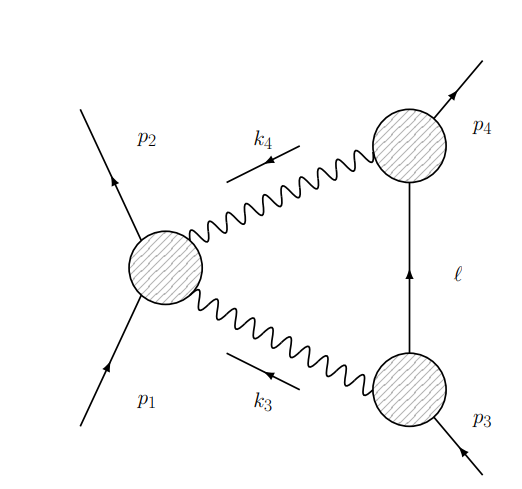
Figure 7.1: Triangle leading-singularity configuration [7]. The gravitational Compton amplitude is glued to two 3 point amplitudes, where the internal lines are on-shell. The Leading singularity corresponds to the loop integration of this amplitude, where internal gravitons are soft as compared to the external massive lines.

This chapter is organized as follows: In section 7.2 we study in more detail amplitudes $A_{n}$ for $n=3.4$ in spinor-helicity variables, and show in the infinite spin limit, they can be arranged in an exponential form, as originally proposed by [58, 60]. In section 7.2.1 we show how to extract the classical information of such amplitudes. For $A_{3}$ we indeed recover the exponential form of the linearized Kerr effective metric, whereas for $A_{4}$ we recover the classical exponential form suggested by the on-shell heavy particle EFT of [60] . In section 7.2.2 we use the classical Compton amplitude to study the low energy limit for the scattering of a gravitational wave off the Kerr BH, up to fourth order in the spin of the BH. Spin induced polarization of the wave after the scattering process is discussed. In section 7.3 we show the classical $A_{4}$ can indeed be used to reproduce the 2PM scattering angle computation of [58]. We leave for appendix F Teukolsky formulation for the scattering of the gravitational wave off Kerr, and argue it agrees with the amplitudes derivation of the present chapter up to fourth order in spin.

This chapter is mainly based on work [84], as well as work in progress [85].

7.2 Exponential 3 and 4 point spinning amplitude

Following [58], and as reviewed in section 1.4, in terms of the angular momentum operator in spinor helicity variables, the gravitational 3-point and 4-point amplitudes can be put into the exponential form (1.57) and (1.59) respectively. For $A_{3}$, in chapter 4 we saw how an analogous formula holds in covariant notation up to quadratic order in spin, and in section 4.3.1 we provided a local form of the 3-point amplitude to all orders in spin in $D=4$. For the 4-point amplitude in covariant form, such exponentiation is not evident, whereas in spinor-helicity variables it is immediate to get as given in (6.47) for the opposite helicity configuration.

In this section we aim to extract the classical limit of amplitudes (1.57) and (1.59), and show they agree with the classical description of the Kerr BH. Let us rewrite explicitly the amplitudes (1.57) and (1.59) for the reader’s convenience

$$A^{S}_{3}=A^{0}_{3}\times\langle\varepsilon_{3}|\exp\left(\frac{F_{2\mu\nu}J^{\mu\nu}}{2i\epsilon_{2}\cdot p_{1}}\right)|\varepsilon_{1}\rangle\,,A^{S}_{4}=A^{0}_{4}\times\langle\varepsilon_{4}|\exp\left(\frac{F_{2,\mu\nu}J^{\mu\nu}}{2i\epsilon_{2}\cdot p_{1}}\right)|\varepsilon_{1}\rangle$$ (7.1)

Recall that the graviton polarization vector is given by $\epsilon_{\mu\nu}=\epsilon_{\mu}\epsilon_{\nu}$ and we have defined $F_{\mu\nu}=2k_{[\mu}\epsilon_{\nu]}$. Let us also use momentum conservation, respectively for the 3-point and 4-point amplitudes as follows:

$$p_{3} = p_{1}+k_{2}$$

$$p_{4} = p_{1}+k_{2}+k_{3}\,.$$ (7.2)

In both cases we assume the graviton associated to $k_{2}$ to have negative helicity, and for $n=4$ the graviton $k_{3}$ has positive helicity. The gauge is fixed, in spinor-helicity variables, as [58]

$$\epsilon_{2}=\frac{\sqrt{2}|3]\langle 2|}{[32]}\propto\tilde{\epsilon}_{3}=\frac{\sqrt{2}|3]\langle 2|}{\langle 32\rangle}\,.$$ (7.3)

The operator $J_{\mu\nu}$ in (7.1) is a Lorentz generator in the spin-$s$ representation. In this case we will realize it as a fully quantum operator acting linearly on the representation $|\varepsilon\rangle$. The exponential series truncates at order $2s$ in the expansion of the exponential. The pole $\epsilon\cdot p$ will cancel in the cases treated here. As anticipated, this effectively restricts $S\leq 2$ in the Compton amplitude $A_{4}$, since as mentioned in section 1.4, unphysical poles, which we shall not discuss in this thesis, arise from the exponent in the 4-point case which cannot be canceled by the scalar amplitude. In previous amplitudes we have introduced a factor of $i$ in the exponent and defined the Lorentz generators with that extra factor.

As explained in section 4.3.1, in order to extract the classical piece of the spinning amplitude, we need to align the polarization states towards the same little group. We therefore introduce a four-velocity vector $u^{\mu}$ together with a generic mass scale $m$. They will be mapped to the four-velocity and rest frame mass of the classical object, respectively. However, the identification with the kinematic momenta in the Compton amplitude is ambiguous, some choices are $u=\frac{p_{1}}{m},\frac{p_{4}}{m},\frac{p}{m}$ (with $m=M$ in the former cases, and $m^{2}=p^{2},p=\frac{p_{1}+p_{4}}{2}$ in the latter), which will all coincide after we take the classical limit. Now, in order to parametrize the degrees of freedom associated with spin in four dimensions we introduce the Pauli-Lubanski operator

$$a^{\mu}:=\frac{1}{2m}\epsilon^{\mu\nu\rho\sigma}u_{\nu}J_{\rho\sigma}$$ (7.4)

This will play the role of the spin vector introduced in previous sections. However, this gives us only a classical relation between $J^{\mu\nu}$ and the spin vector $a^{\mu}$. Using spinor-helicity variables we can find an exact quantum relation between operators. For this, note that in (7.1) the field strength $F_{2}^{\mu\nu}$ is self-dual since the graviton $k_{2}$ has negative helicity. Consequently, the generator $J_{\mu\nu}$ is also self-dual and it is associated with the chiral basis (1.50), i.e. $J^{\mu\nu}=\frac{i}{2}\epsilon^{\mu\nu\rho\sigma}J_{\rho\sigma}$. We use this property to rewrite the exponents of (7.1) in terms of the spin vector (7.4) as follows. Following the discussion of section 4.3.1 , for a given 4-velocity $u^{\mu}$ we decompose the full Lorentz generator $J^{\mu\nu}$ into a spin and a boost operator:

$$B^{\mu}:=J^{\mu\nu}u_{\nu}\,,\qquad S^{\mu\nu}:=J^{\mu\nu}-2u^{[\mu}B^{\nu]}\,.$$ (7.5)

One can easily check that $u_{\mu}S^{\mu\nu}=0$, hence $S^{\mu\nu}$ generates little group transformations on states $|\varepsilon\rangle$ and shall be related to the Pauli-Lubanski vector $a^{\mu}$. Indeed, from (7.4) one easily finds

$$a^{\mu}=\frac{1}{2m}\epsilon^{\mu\nu\rho\sigma}u_{\nu}S_{\rho\sigma}\Leftrightarrow S^{\mu\nu}=-m\epsilon^{\mu\nu\rho\sigma}u_{\rho}a_{\sigma}\,.$$ (7.6)

Furthermore, due to the self-dual condition on $J^{\mu\nu}$, it turns out that the boost and spin parts are indeed related. From (7.4) and (7.5) we find:

$$B^{\mu}=ima^{\mu}\,.$$ (7.7)

We can now decompose the exponent of (7.1). We proceed for both $n=3,4$ at the same time, introducing the generic field strength $F_{\mu\nu}=2k_{[\mu}\epsilon_{\nu]}$. Using (7.6) and (7.7) we have

$$F_{\mu\nu}J^{\mu\nu} = F_{\mu\nu}S^{\mu\nu}+2u_{\mu}F^{\mu\nu}B_{\nu}$$ (7.8)

$$= -m\,\epsilon^{\mu\nu\rho\sigma}F_{\mu\nu}u_{\rho}a_{\sigma}+2im\,u_{\mu}F^{\mu\nu}a_{\nu}\,.$$

Regarding $F_{\mu\nu}$ as self dual, which follows from the contraction with $J^{\mu\nu}$ on the LHS, we finally get

$$F_{\mu\nu}J^{\mu\nu}=\\ ac{PM}4im\,u_{\mu}F^{\mu\nu}a_{\nu}\,.$$ (7.9)

The $\pm$ sign accounts for self-duality or anti self-duality of the Lorentz generator $J_{\mu\nu}$, or equivalently, the helicity associated to $F_{\mu\nu}$. We remark that the classical limit has not yet been applied. Note that the LHS does not depend on the four-vector $u^{\mu}$, which we are free to choose. In any case, for $u=\frac{p_{1}}{M},\frac{p_{4}}{M},\frac{p}{m}$ we can now rewrite (7.1) as

$$A^{S}_{3}=A^{0}_{3}\times\langle\varepsilon_{3}|\exp\left(2\frac{u\cdot F_{2}\cdot a}{u\cdot\epsilon_{2}}\right)|\varepsilon_{1}\rangle\,,A^{S}_{4}=A^{0}_{4}\times\langle\varepsilon_{4}|\exp\left(2\frac{u\cdot F_{2}\cdot a}{u\cdot\epsilon_{2}}\right)|\varepsilon_{1}\rangle$$ (7.10)

For $n=3$ we have $u\cdot k_{2}=0$ from the on-shell conditions. This automatically implies that the pole $u\cdot\epsilon_{2}$ cancels and we have

$$A^{S}_{3}=A^{0}_{3}\times\langle\varepsilon_{3}|e^{-2k_{2}\cdot a}|\varepsilon_{1}\rangle\,.$$ (7.11)

For $n=4$, the pole does not cancel in the exponential, as $u\cdot k_{2}\neq 0$ generically. Since the prefactor $A_{4}^{0}$ contains a term $(u\cdot\epsilon_{2})^{4}$, the form (7.10) is valid only up quartic order in the expansion of the exponential, i.e. up to spin $S=2$. We can encode the unphysical pole in the vector

$$w^{\mu}:=\frac{u\cdot k_{2}}{u\cdot\epsilon_{2}}\epsilon^{\mu}_{2}\,,$$ (7.12)

so that

$$A^{S}_{4}=A^{0}_{4}\times\langle\varepsilon_{4}|e^{2(w\cdot a-k_{2}\cdot a)}|\varepsilon_{1}\rangle\,.$$ (7.13)

The polarization states $|\varepsilon_{1}\rangle,\langle\varepsilon_{4}|$ are associated with initial and final momentum, $p_{1},p_{4}$ respectively. It will be convenient to rewrite them as associated to the 4-velocity $u^{\mu}$. For instance, taking $u=\frac{p_{1}}{M}$, we can write

$$p_{4}=e^{i\mu M(k_{2}+k_{3})\cdot B}p_{1}=e^{-\mu M^{2}(k_{2}+k_{3})\cdot a}p_{1}\,,$$ (7.14)

Here $\mu$ is a scalar which explicit expression we do not need, but which is given explicitly in [59]. The analogous formula holds for $n=3$; in this case three-particle kinematics yields $\mu M^{2}=1$, hence

$$p_{3}=e^{-k_{2}\cdot a}p_{1}\,,$$ (7.15)

This implies that we can write

$$|\varepsilon_{3}\rangle = e^{-k_{2}\cdot a}|\varepsilon^{\prime}_{1}\rangle\,,\qquad\,\,\qquad n=3$$ (7.16)

$$|\varepsilon_{4}\rangle = e^{-\mu M^{2}(k_{2}+k_{3})\cdot a}|\varepsilon^{\prime}_{1}\rangle\,,\quad n=4$$ (7.17)

where $|\varepsilon^{\prime}_{1}\rangle$ is a polarization state associated to $p_{1}=Mu$. Thus we have the following QFT amplitudes

$$A^{S}_{3}=A^{0}_{3}\times\langle\varepsilon^{\prime}_{1}|e^{k_{2}\cdot a}e^{-2k_{2}\cdot a}|\varepsilon_{1}\rangle=A^{0}_{3}\times\langle\varepsilon^{\prime}_{1}|e^{-k_{2}\cdot a}|\varepsilon_{1}\rangle\,,$$ (7.18)

and

$$A^{S}_{4}=A^{0}_{4}\times\langle\varepsilon^{\prime}_{1}|e^{\mu M^{2}(k_{2}+k_{3})\cdot a}e^{2(w-k_{2})\cdot a}|\varepsilon_{1}\rangle\,.$$ (7.19)

The constraint $u\cdot a=0$ implies that the Pauli-Lubanski vector $a^{\mu}$ only yields three independent operators. In the rest frame of $u^{\mu}$ they satisfy $[a^{i},a^{j}]=\epsilon^{ijk}a_{k}$, or covariantly

$$[a^{\mu},a^{\nu}]=M^{-1}S^{\mu\nu}=\epsilon^{\mu\nu\rho\sigma}a_{\rho}u_{\sigma}\,.$$ (7.20)

In eq. (7.18) only the combination $k_{2}\cdot a$ appears. Furthermore, note that in this case the boost component $e^{k_{2}\cdot a}$ commutes with the amplitude $e^{-2k_{2}\cdot a}$. This is not the case for eq. (7.19) where indeed all three combinations $k_{2}\cdot a,k_{3}\cdot a,w\cdot a$ appear and do not commute. As the spin is the only quantum number available, we assume that in general these combinations span a basis of operators in the space of states associated to $u^{\mu}$, namely $|\varepsilon_{1}\rangle,\langle\varepsilon^{\prime}_{1}|$.

7.2.1 Classical Limit

As argued in the previous section, the operator $O$ in the contraction $\langle\varepsilon^{\prime}_{1}|O|\varepsilon_{1}\rangle$ can be attributed a classical nature. We note that the three-point amplitude (7.18) is invariant under such limit

$$\boxed{\langle A_{3}^{S}\rangle=\langle A_{3}^{0}\rangle e^{-k_{2}\cdot a},}$$ (7.21)

whereas for the four-point (7.19) we obtain

$$w^{\mu},k_{2}^{\mu},k_{3}^{\mu}\sim\hbar\,,\quad a^{\mu}\sim 1/\hbar\,.$$ (7.22)

where the scaling of $w^{\mu}$ follows from its definition (7.12). Together (7.20) this implies

$$[(k_{2}+k_{3})\cdot a,(w-k_{2})\cdot a]\sim\hbar$$ (7.23)

i.e. the exponents of (7.19) commute in the classical limit. Furthermore, from the explicit expression in [59] we see that $\mu M^{2}=1+\mathcal{O}(\hbar)$, hence the limit of (7.19) becomes

$$A^{S}_{4}=A^{0}_{4}\times\langle\varepsilon^{\prime}_{1}|e^{(2w+k_{3}-k_{2})\cdot a}|\varepsilon_{1}\rangle+\mathcal{O}(\hbar)\Longrightarrow\boxed{\langle A^{S}_{4}\rangle=\langle A^{0}_{4}\rangle\times e^{(2w+k_{3}-k_{2})\cdot a}\,.}$$ (7.24)

This result agrees with the one obtained in [60] from Heavy Particle EFT. This is expected since we have argued in [84] that the limits $\hbar\to 0$ and $M\to\infty$ are equivalent. Note that in the last step of (7.24) we have stripped off the polarization states $|\varepsilon_{1}\rangle,|\varepsilon^{\prime}_{1}\rangle$. In this case, $a^{\mu}$ is interpret as a classical spin-vector and not an operator.

In an analogous way, one can show that the classical limit for the same helicity configuration of the gravitational Compton amplitude is simply given by

$$\boxed{\langle\tilde{A}_{4}^{S}\rangle=\langle\tilde{A}_{4}^{0}\rangle e^{(k_{3}+k_{2}){\cdot}a}\,.}$$ (7.25)

which agrees with the result of [60] from Heavy Particle EFT.

7.2.2 Gravitational wave scattering

Amplitude (7.21) precisely agrees with the exponentiated spin structure of the linearized Kerr metric as shown in the seminal work [58]. The natural question to ask is, what does $A_{4}$ have to do with the Kerr BH? In the follows, and in appendix F we will argue that (7.24) corresponds to a effective description of the low energy regime of the a gravitational wave scattering off the Kerr BH.

For that let us consider the gravitational analog of the Thomson scattering process in QED as reviewed in chapter 2. In Figure 7.2 (right) we do a schematic representation of the process from an amplitudes perspective (see also Figure 2.1): A wave of helicity $h=2$ is scattered off the Kerr BH.

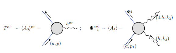
Figure 7.2: Left: Schematic representation of the correspondence between the spin multiple moments of the Kerr BH and the minimal coupling $3$ pt amplitude. Right: Graphic representation for the scattering of a plane wave of helicity $h$, off the Kerr BH.

In terms of the kinematics (2.9) in the classical limit, and using a generic orientation for the spin vector $a^{\mu}=(0,a_{x},a_{y},a_{z})$, in the BH rest frame, amplitudes (7.24) and (7.25) become

$$\langle A_{4}^{++}\rangle =\frac{\kappa^{2}M^{2}\cos^{4}(\theta/2)}{4\sin^{2}(\theta/2)}\big{[}1+\mathcal{F}(\omega,a,\theta)+\frac{1}{2!}\mathcal{F}(\omega,a,\theta)^{2}+\frac{1}{3!}\mathcal{F}(\omega,a,\theta)^{3}+\frac{1}{4!}\mathcal{F}(\omega,a,\theta)^{4}\big{]}\,,$$ (7.26)

$$\langle A_{4}^{--}\rangle =\left[\langle A_{4}^{++}\rangle^{*}\right]_{\omega\rightarrow-\omega}\,,$$ (7.27)

$$\langle A_{4}^{+-}\rangle =\frac{\kappa^{2}M^{2}\sin^{4}(\theta/2)}{4\sin^{2}(\theta/2)}\big{[}\mathcal{G}(\omega,a,\theta)+\frac{1}{2!}\mathcal{G}(\omega,a,\theta)^{2}+\frac{1}{3!}\mathcal{G}(\omega,a,\theta)^{3}+\frac{1}{4!}\mathcal{G}(\omega,a,\theta)^{4}\big{]}\,\,,$$ (7.28)

$$\langle A_{4}^{-+}\rangle =\left[\langle A_{4}^{+-}\rangle^{*}\right]_{\omega\rightarrow-\omega}\,,$$ (7.29)

where we have truncated the expansion at $a^{4}$ ($S=2$), where the Compton amplitude has physical meaning, and we have further used

$$\mathcal{F}(\omega,a,\theta) = -2a_{z}\omega\sin^{2}(\theta/2)+a_{x}\omega\sin\theta-2(a_{x}-ia_{y})\omega\tan(\theta/2)\,,$$ (7.30)

$$\mathcal{G}(\omega,a,\theta) = 2a_{z}\omega\sin^{2}(\theta/2)-a_{x}\omega\sin\theta\,.$$ (7.31)

which come naturally from rewriting the exponent in (7.24) and (7.25) respectively, in terms of the scattering angle, using kinematics (2.9). We have in addition written all of the helicity configurations entering into the scattering matrix (2.16), which follow from changing the direction of the massless momenta. Up to $a^{2}$, one can easily show that the same result can be obtained starting from the quadratic in spin classical Compton amplitude derived from the covariant spin multipole double copy, and written in vector notation in (4.54), once we use (2.17) and (2.18) as the polarization states for the incoming and outgoing wave, respectively, and the kinematics (2.9) in the classical limit. This provides a strong consistency check for the amplitudes written in both, vector and spinor notation, and the validity of the spin multipole double copy introduced in chapter 4.

Using (2.15) we can then compute the unpolarized differential for the scattering of gravitational waves off the Kerr BH. Up to quartic order in spin it is simply given by

$$\begin{split}\frac{d\braket{\sigma}}{d\Omega}&=\frac{G^{2}M^{2}}{\sin^{4}(\theta/2)}\Big{[}\cos^{8}(\theta/2)\Big{(}1+2\tilde{\mathcal{F}}+\frac{(2\tilde{\mathcal{F}})^{2}}{2!}+\frac{(2\tilde{\mathcal{F}})^{3}}{3!}+\frac{(2\tilde{\mathcal{F}})^{4}}{4!}\Big{)}\\ &\qquad\qquad\qquad+\sin^{8}(\theta/2)\Big{(}1+2\mathcal{G}+\frac{(2\mathcal{G})^{2}}{2!}+\frac{(2\mathcal{G})^{3}}{3!}+\frac{(2\mathcal{G})^{4}}{4!}\Big{)}\Big{)}\Big{]}+\mathcal{O}(a^{5})\,,\end{split}$$ (7.32)

where $\tilde{\mathcal{F}}=\mathcal{F}\big{|}_{a_{y}=0}$, and we have used $\kappa^{2}=32\pi G$. We then see the $a_{y}$ component of the spin corresponds to just a phase in the amplitude, unimportant for the cross section, as one could have guessed from the exponential structure of the amplitude. Interestingly, the only spin components contributing to the actual observables are those with non zero projection on the scattering plane.

The first difference we notice when comparison to the Thomson differential cross section for the scattering of electromagnetic waves off charge compact objects (2.21) (set $f,g\to 0$ for the moment) is that unlike for the latter, (7.32) does diverge in the $\theta\to 0$ limit. This is a forward divergence and is due to the long range nature of the gravitational potential. There is a second difference when spin is included, which manifests in a spin induced polarization of the incoming wave as we now discuss.

7.2.3 Spin-induced Polarization

In general, incoming waves can be linearly polarized, that is, they can be written as a superposition of circularly polarized waves. When impinging on the black hole, waves of different circular polarization can scatter by a different angle. This in turn will induce a polarization of the wave after scattering, which will be reflected in the difference between elements of the scattering matrix (2.16). To see this explicitly we compare the scattering cross-sections for a left ($+$) and right ($-$) circularly polarized incoming wave:

$$\begin{split}64\pi^{2}M^{2}\frac{d\langle\sigma_{+}\rangle}{d\Omega}&=\langle A_{++}\rangle\langle A_{++}\rangle^{*}+\langle A_{+-}\rangle\langle A_{+-}\rangle^{*}\\ 64\pi^{2}M^{2}\frac{d\langle\sigma_{-}\rangle}{d\Omega}&=\langle A_{--}\rangle\langle A_{--}\rangle^{*}+\langle A_{-+}\rangle\langle A_{-+}\rangle^{*}\end{split}$$ (7.33)

We have found from (7.26-7.29) that opposite helicity amplitudes are related via $\langle A\rangle\to\langle A\rangle^{*}$, accompanied by the expected time reversal $\omega\to-\omega$, map. This is more transparent in the spinor-helicity formalism, and can be seen as a consequence of CPT/crossing symmetry: Opposite helicities are related by chiral (i.e. complex) conjugation in the amplitude. This induces a parity transformation which flips the sign of $a^{\mu}$, which corresponds to a pseudovector as it describes the orientation of the rotating black hole. Due to the fact that spin only enters through the combination $a\omega$ the map $a^{\mu}\to-a^{\mu}$ is of course equivalent to $\omega\to-\omega$.

From the above discussion, using (7.33), we easily conclude that

$$\frac{d\langle\sigma_{+}\rangle}{d\Omega}=\left[\frac{d\langle\sigma_{-}\rangle}{d\Omega}\right]_{(\omega\to-\omega)}$$ (7.34)

Following [331, 127, 129] we also introduce the polarization measurement

$$\mathcal{P}=\frac{\frac{d\langle\sigma_{+}\rangle}{d\Omega}-\frac{d\langle\sigma_{-}\rangle}{d\Omega}}{\frac{d\langle\sigma_{+}\rangle}{d\Omega}+\frac{d\langle\sigma_{-}\rangle}{d\Omega}}\,.$$ (7.35)

According to (7.34) the numerator of the polarization depends only on odd powers of $a\omega$ in the cross-section, and in particular vanishes for the Schwarzschild case. Let us for simplicity restrict here to the polar scattering case, where the impinging wave moves along the direction of the spin of the BH, i.e. $a_{x}=a_{y}=0$. Let us also consider the linear in spin term. Extension to general spin orientation is straightforwards to compute using the full expression for the differential cross section (7.32). In this case, the spin induced polarization simply reads

$$\mathcal{P}=-\left(4a_{z}|\omega|\sin^{2}(\theta/2)\right)\frac{\cos^{8}(\theta/2)-\sin^{8}(\theta/2)}{\cos^{8}(\theta/2)+\sin^{8}(\theta/2)}\,,$$ (7.36)

which for $\theta\rightarrow 0$ becomes $\mathcal{P}=-a_{z}|\omega|\theta^{2}$ and thus recovers the classical result using BHPT [127] (see also appendix F). It however disagrees with the prediction of [128, 129] to linear order in spin. The reason for this mismatch is that [128, 129] only considered the graviton exchange diagram between the wave and the BH, whereas in here we have shown in order to recover the classical result computed BHPT, one needs to consider the full classical gravitational Compton amplitude. Indeed, in appendix F we argue the cross section (7.32) indeed matches in a spectacular way the classical result obtained by solving the Teukolsky equation. This then allows us to conclude confidently the minimal gravitational Compton amplitude is indeed a equivalent description of the scattering of gravitational waves off the Kerr BH. Let us stress this is the first time a direct connection between the classical piece of the gravitational Compton amplitude and the Kerr BH is made. Up to linear order in spin, the wave scattering process is independent whether the compact object corresponds to a Kerr BH or any other spinning of object; by the fact the results for the spin monopole and dipole are universal. However, at quadratic and higher order in spins, the minimal coupling Compton amplitude uniquely describes Kerr BH and not any other compact object, due to its unique spin multipole structure.

7.3 2PM Scattering Angle and the Holomorphic Classical Limit

Let us in the remaining of this chapter show the classical result for the gravitational Compton amplitude can indeed be used to derive the aligned spin scattering angle for the scattering of two Kerr BHs, at order $G^{2}$ and up to $a^{4}$. This will recover the result obtained from the Holomorphic Classical Limit (HCL) computation in [58].

Our aim is to compute the triangle leading singularity of Figure 7.1

$$\mathcal{M}_{4}=\frac{i}{8m_{b}\sqrt{-t}}\int_{\Gamma_{\rm{LS}}}\frac{dy}{2\pi y}\langle A_{4}^{(s_{a})}(P_{1},-P_{2},k_{3}^{+},k_{4}^{-})\rangle\langle A_{3}^{(s_{b})}(P_{3},-l,-k_{3}^{-})\rangle\langle A_{3}^{(s_{b})}(-P_{4},l,-k_{4}^{+})\rangle.$$ (7.37)

where the brackets indicate that we take the classical limit of the indicated amplitudes. It gives the scattering angle via the two dimensional Fourier transform from momentum space $k_{\perp}=(k_{3}-k_{4})_{\perp}$ to impact parameter space $b_{\perp}$ (see eq. $(1.11)$ in [58]). The reason we can reproduce the HCL computation starting from the classical amplitudes is that as it turns out, the HCL (i.e. $\beta\rightarrow 1$ below) is contained in the classical limit, and it corresponds to the special case where the momenta for the two internal gravitons become proportional to each other; this then implies that $k_{2}\,\alpha\,k_{3}\,\alpha\,w$, which in turn makes the basis for the spin directions with $3$ elements to get degenerated to include only one element, which corresponds to the direction in which the spins of the two BHs are aligned.

Let us start our computation by considering that the two incoming black holes have momenta $P_{1}$ and $P_{3}$ and spin $a_{a}$ and $a_{b}$, respectively; likewise, the outgoing BHs will have momentum $P_{2}$ and $P_{4}$, with their spins unchanged. The HCL parametrization for the momenta of the massive particles in the center of mass frame is [57, 103]

$$\begin{split}P_{1}&=|\hat{\eta}]\bra{\hat{\lambda}}+|\hat{\lambda}]\bra{\hat{\eta}},\\ P_{2}&=\beta^{\prime}|\hat{\eta}]\bra{\hat{\lambda}}+\frac{1}{\beta^{\prime}}|\hat{\lambda}]\bra{\hat{\eta}}+|\hat{\lambda}]\bra{\hat{\lambda}},\\ P_{3}&=|\eta]\bra{\lambda}+|\lambda]\bra{\eta},\\ P_{4}&=\beta|\eta]\bra{\lambda}+\frac{1}{\beta}|\lambda]\bra{\eta}+|\lambda]\bra{\lambda},\\ K&=-|\hat{\lambda}]\bra{\hat{\lambda}}+\mathcal{O}(\beta-1)=|\lambda]\bra{\lambda}+\mathcal{O}(\beta^{\prime}-1),\end{split}$$ (7.38)

where $K$ is the complex momentum transfer. The on-shell conditions $P_{1}^{2}=P_{2}^{2}=m_{a}^{2}$ and $P_{3}^{2}=P_{4}^{2}=m_{b}^{2}$, impose the normalization for the spinors $\braket{\hat{\lambda}\hat{\eta}}=[\hat{\lambda}\hat{\eta}]=m_{a}$ and $\braket{\lambda\eta}=[\lambda\eta]=m_{b}$. For the internal gravitons the spinor helicity variables read

$$\begin{split}\ket{k_{2}}&=\frac{1}{\beta+1}\left(\left(\beta^{2}-1\right)\ket{\eta}-\frac{1+\beta y}{y}\ket{\lambda}\right),\,\,\,|k_{2}]=\frac{1}{\beta+1}\left(\left(\beta^{2}-1\right)y|\eta]+(1+\beta y)|\lambda]\right),\\ \ket{k_{3}}&=\frac{1}{\beta+1}\left(\frac{\beta^{2}-1}{\beta}\ket{\eta}+\frac{1-y}{y}\ket{\lambda}\right),\,\,\,|k_{3}]=\frac{1}{\beta+1}\left(-\beta\left(\beta^{2}-1\right)y|\eta]+(1-\beta^{2}y)|\lambda]\right).\end{split}$$ (7.39)

We define the variables $U$, $V$ and $\gamma$ from the massive momenta as follows

$$\begin{split}U&=[\lambda|P_{1}\ket{\eta},\\ V&=[\eta|P_{1}\ket{\lambda},\\ \gamma&=\frac{P_{1}\cdot P_{3}}{m_{a}m_{b}}=\frac{1}{\sqrt{1-v^{2}}},\end{split}$$ (7.40)

which satisfy the useful identities [103] :

$$\begin{split}[\lambda|P_{1}\ket{\lambda}&=-\frac{(\beta-1)^{2}}{\beta}m_{b}^{2}+(1-\beta)V+\frac{\beta-1}{\beta}U,\\ [\eta|P_{1}\ket{\eta}[\lambda|P_{1}\ket{\lambda}&=UV-m_{a}^{2}m_{b}^{2}.\end{split}$$ (7.41)

The HCL is achieved by taking $\beta\rightarrow 1$ (or equivalently $\beta^{\prime}\rightarrow 1$). In this limit, the variables $U$ and $V$ are related to $v$ via

$$\begin{split}U&=m_{a}m_{b}(1-v)\gamma,\\ V&=m_{a}m_{b}(1+v)\gamma.\end{split}$$ (7.42)

To evaluate the LS (7.37), let us consider first the non spinning piece of the amplitudes entering in the integral. The classical piece for the scalar Compton amplitude (1.60), in the gauge (7.3), is simply given by

$$\langle A_{4}^{0}(P_{1},-P_{2},k_{3}^{+},k_{4}^{-})\rangle=32\pi Gm_{a}^{2}\frac{(\epsilon_{2}\cdot u)^{2}(\tilde{\epsilon}_{3}\cdot u)^{2}}{\langle\xi\rangle},\,\,\,\langle\xi\rangle=\frac{(s_{c}-m_{a}^{2})^{2}}{m_{a}^{2}t}$$ (7.43)

where $s_{c}=(P_{1}+k_{2})^{2}$, and $t=(P_{1}-P_{2})^{2}$, i.e. the t-channel for the Compton amplitude coincides with that for the massive 4-pt amplitude. We have taken the classical limit of the optical parameter $\xi$ as given in (2.12) by means of the classical identity (2.11). In the HCL the Compton Mandelstam invariants read

$$\begin{split}s_{c}&=m_{a}^{2}-m_{a}m_{b}\gamma\frac{y^{2}-1}{2y}(\beta-1)\,,\\ t&=m_{b}^{2}\frac{(\beta-1)^{2}}{\beta}\,.\end{split}$$ (7.44)

Then, we can easily check that in the HCL parametrization (7.38) and (7.39):

$$\langle\xi\rangle\rightarrow-\gamma^{2}v^{2}\frac{(1-y^{2})^{2}}{4y},$$ (7.45)

and in the gauge (7.3), the scalar classical Compton amplitude becomes

$$\langle A_{4}^{0}(P_{1},-P_{2},k_{3}^{+},k_{4}^{-})\rangle=32\pi Gm_{a}^{2}\frac{(2y-v(1+y^{2}))^{4}\gamma^{2}}{16v^{2}y^{2}(1-y^{2})^{2}}.$$ (7.46)

In the same way, it is straightforwards to see that in the HCL, the scalar piece of the 3-pt amplitudes evaluates to

$$\langle A_{3}^{0}(P_{3},-l,-k_{3}^{-})\rangle\langle A_{3}^{0}(-P_{4},l,-k_{4}^{+})\rangle=8\pi Gm_{b}^{4}.$$ (7.47)

We now turn our attention to the spinning pieces of the amplitudes. For that, it is useful to write the classical spin vector for the BHs in terms of the $SL(2,C)$ sigma matrices

$$(S^{\mu})_{\alpha}^{\,\,\beta}=\frac{1}{4}\left[(\sigma^{\mu})_{\alpha\dot{\alpha}}u^{\dot{\alpha}\beta}-u_{\alpha\dot{\alpha}}(\bar{\sigma}^{\mu})^{\dot{\alpha}\beta}\right]+\mathcal{O}(\hbar),$$ (7.48)

where as mentioned before, $u$ can be chosen to be the velocity of the initial or the final BH, or the average velocity. Quantum mechanical corrections arise if we include contributions to $u$ coming from the gravitons momenta.

Let us choose for instance $u=\frac{P_{1}}{m_{a}}$. Then, using (7.12) as the definition for $\omega^{\mu}$, and the kinematics in the HCL (7.38 - 7.39), together with (7.48), it is straightforward to show that to leading order in $1-\beta$, the classical basis of spin $\{\omega\cdot a,k_{2}\cdot a,k_{3}\cdot a\}$ maps to

$$\begin{split}w&\rightarrow iK\frac{v\left(1-y^{2}\right)^{2}}{4y\left(v-2y+vy^{2}\right)}\\ k_{2}&\rightarrow iK\frac{(1+y)^{2}}{4y},\\ k_{3}&\rightarrow-iK\frac{(1-y)^{2}}{4y},\end{split}$$ (7.49)

note that in the HCL $k_{3}-k_{2}=K=|\lambda\rangle[\lambda|$, which turns take the exponential piece in (7.24) into

$$e^{(2w+k3-k2)\cdot a_{a}}\rightarrow e^{-i\frac{1+y^{2}-2vy}{2y-v(1+y^{2})}K\cdot a_{a}},$$ (7.50)

and analogous the product of two exponential for the 3-pt amplitudes (7.21) becomes

$$e^{-2k_{2}\cdot a_{b}}\rightarrow e^{-i\frac{(1+y^{2})}{2y}K\cdot a_{b}}.$$ (7.51)

Putting all these ingredients together, the LS (7.37) evaluates to

$$\frac{i2\pi^{2}G^{2}m_{a}^{2}m_{b}^{3}\gamma^{2}}{v^{2}\sqrt{-t}}\int_{\Gamma_{\rm{LS}}}\frac{dy[2y-v(1+y^{2})]^{4}}{2\pi y^{3}(1-y^{2})^{2}}\exp\left(-i\frac{1+y^{2}-2vy}{2y-v(1+y^{2})}K{\cdot}a_{a}-i\frac{(1+y^{2})}{2y}K{\cdot}a_{b}\right),$$ (7.52)

which recovers the result of [58] up to $a_{a}^{4}$. The evaluation of the integral was done in the same reference.

As last comment, in principle in the computation of the leading singularity in Figure 7.1, a sum over the exchange graviton polarization is needed. This means, the same helicity Compton amplitude (7.25) needs to be included in the computation. One can however check explicitly such configuration produces vanishing contribution to the scattering angle in the aligned spin setup.

7.4 Outlook of the chapter

In this chapter we have argued the minimal coupling classical amplitudes $A_{n}$ for $n=3,4$ are indeed very related to the Kerr BH by means of the unique spin multipole structure fixed for minimal coupling amplitudes, which map directly to the spin multipole moments of the Kerr BH. This matching further clarifies the mismatch between the Feynman diagram prediction for the spin induced polarization made by Barbieri and Guadagnini [128, 129] to those of BHPT by Dolarn [127] at linear order in spin. In particular, the spin induced polarization, had the simple pattern for haves of helicity $h<2$

$$\mathcal{P}^{(h)}=-h\sinh{\left(4a_{z}|\omega|\sin^{2}(\theta/2)\right)}\left[\cosh^{2}{\left(2a_{z}|\omega|\sin^{2}(\theta/2)\right)}+h^{2}\sinh^{2}{\left(2a_{z}|\omega|\sin^{2}(\theta/2)\right)}\right]^{-1},$$ (7.53)

as computed by the author of this thesis and collaborators in [84], which for $\theta\rightarrow 0$ is simply $\mathcal{P}^{(h)}=-ha_{z}|\omega|\theta^{2}$, disagrees with the BHPT result (7.36) if extrapolated to $h=2$. The solution to this disagreement is of course to include the additional diagrams that restore gauge invariance of the amplitude. Result (7.53) recovers those in [331, 129] for $h<2$ at linear order in spin, which needed only from the one graviton exchange diagram.

In appendix F we check explicitly amplitudes (7.26) and (7.28) match exactly the classical result for the scattering of a gravitational wave off the Kerr BH, using BHPT. Amplitudes computed from this QFT approach are written in a closed form which in turn re-sums the infinite sums appearing from the partial wave expansion as required from usual classical wave physics.

For spin $S>2$, amplitude (7.24) needs to be modified. In particular, the unphysical poles arising from $w{\cdot}a$, can be removed by adding contact terms with unfixed coefficients. In [85] it was shown that by matching to higher spin solutions of the Teukolsky equation, these coefficients can be fixed for the Kerr BH. Explicit results up to spin $S=3$ are provided, but their interpretation are beyond the scope of this thesis. The BHPT solutions however disagree with the recent proposal in [91], where the free coefficients of an ansatz for the higher spin gravitational Compton amplitude were fixed by imposing that for the conservative 2PM binary black hole amplitude, certain spin structure observed at lower spins, is conserved (see also [90]).

Chapter 8 General Discussion

In this thesis we have presented a study addressing the computation of classical observables in classical gauge theories and gravity directly from the classical limit of QFT amplitudes, using modern amplitudes techniques such as double copy [135, 67, 144], spinor-helicity variables [160, 152, 68], leading singularities and the HCL [57, 58], the KMOC formalism [78, 78, 130, 59, 131, 132, 93], the amplitudes to the Kerr BH correspondence [103, 58, 104, 84, 85]. We have presented a detail study of amplitudes for a massive spinning line emitting photons/graviton, $A_{n}$, both in (S)QED (QCD) and Gravity as they are the main building blocks to compute two-body observables at leading and subleading orders in perturbation theory. Such building blocks possess many remarkable properties such as soft exponentiation, universal covariant spin multipole expansion, multipole preserving double copy, healthy high energy limit due to the fact they can be constructed from dimensional reduction and compactifications arguments, and they are not polluted with additional massless degrees of freedom (dilaton, axion) from the double copy. In addition, we have shown the classical limit of $A_{n}$ amplitudes can be directly associated to represent classical processes in both electrodynamics and general relativity. For $n=3$, and in the (electromagnetic) gravitational case, this amplitude encodes the same spin multipole structure of the (root) Kerr BH, as shown by the seminal work of [103, 58, 104]. The $n=4$ case on the other hand, describes the low energy limit for the scattering of waves off classical compact objects with and without spin structures. For instance, in the electromagnetic case, $A_{4}$ recovers results for the differential cross section for the well known Thompson process, whereas for gravity, $A_{4}$ encodes the information for the scattering of gravitational waves off the Kerr BH. This in turn open a new amplitudes-BHPT correspondence [84, 85] , allowing to study complicated gravitational scattering problems from simple QFT derivations.

We presented a detailed study of amplitudes in the electromagnetic theory, and show how soft theorems provide an infinite tower of constraints on the KMOC formula for the computation of radiation. These constraints can naturally be generalized to the gravitational theory and extended to subleading orders in the soft expansion [109]. Understanding soft radiation is important since it encodes the so called Gravitational Memory Effect (GME), as dictated by the infrared triangle [219]. This is a strong gravity effect and although it has not yet been detected in the current GW observatories, preliminary analysis [332] of available data from the LIGO/VIRGO GW catalog suggest that GME is very likely to be observed in the era of the advance LIGO/VIRGO detector, where an order of $2000$ events will be needed to say something conclusive. In addition, positive LISA prospects for measuring of the GME from the coalescing of super massive BH even at red-shift values of $\sim 5$ for BHs masses of order $10^{5}-10^{6}M_{\odot}$ are expected [15]. Furthermore, soft theorems being non perturbative can give information about radiation, and radiation reaction to higher orders in perturbation theory [178, 172, 173, 179, 177, 53, 77, 111, 112, 109]. On the other hand, studding electromagnetic radiation rather than color radiation, simplifies the computations as it avoids the complications introduced by the non abelian character the colour group, and permits to obtain two-body gravitational radiation from KLT double copy properties of $A_{n}$ theories at lower orders in perturbation theory, which at the same time permits to easily remove extra degrees of freedom product of the double copy.

Inspired by the early work of Holstein [188, 207], Vaidya [196], Cachazo and Guevara [57, 7] for the study of spin effects in the conservative sector of the two body problem from minimal coupling amplitudes (see also [103, 58] ), we have introduced a detailed study for inclusion of spin effects in the electromagnetic and gravitational theories for the radiative sector, as well as for one-body wave scattering processes through the spin multipole double copy. Results for lower orders in the covariant spin multipolar expansion naturally recover results from classical worldline computations [80, 80, 6, 117], and extend them quadrupolar order. Extraction of the spin structure from QFT amplitudes in a vector notation in general is a non-trivial task, and it is therefore more suitable to use spinor-helicity variables for such endeavors, as we have exemplified through several parts of the body of this thesis, in particular, in the identification of Compton amplitude with low energy solutions of the Teukoslky equation in chapter 7 and appendix F. Additional approaches to include spin effects in vector notation such as the EFT formulation of spin [54] or the worldline theory [197, 333, 334, 328, 256, 120, 335, 89] are also techniques of current use. Studying spin effects is important since they encode information regarding the formation mechanism of the binary system (see for instance [113, 114, 115]), and for nearly extremal Kerr BHs, the individual spins of the binary’s components are expected to be measured with great precision by LISA [116].

Motivated by the non-universality of the bounded-unbounded character of the two-body problem [97, 4], we initiated the program of computing classical observables for systems in bounded orbits directly from scattering amplitudes. Formulas for the radiated field were motivated by the classical worldline computation [31] and the Feynman diagrammatic approach of [121], but we argued they can be seen as a promotion of KMOC formalism to include generic particles trajectories. It is desirable to probe these formulas from first principles as they could naturally account for radiation reaction forces captured by the conservative amplitude (and therefore by the bodies EoM), which are added from balance equations arguments to the objects’ EoM in the EOB formalism when addressing the radiative sector [95]. Guidance from the Worldline QFT [233], or the in-in formalism [336, 336, 337, 338], might be of great use in this endeavor. In addition, it would be interesting to establish a precise dictionary between the soft expansion and the source multipole decomposition for the bounded orbit problem. The reason for this is that soft theorems are non perturbative and therefore encode all orders in perturbation theory, and higher velocity corrections to the waveform, as dictated by the virial theorem.

On the formal side of the double copy for spinning matter, we have shown how graviton coupling to matter produce universal term in the Lagrangian description, whereas coupling of additional double copy states such as dilaton and two-form field have non universal coupling. This led us to identify two independent double copy theories producing spin 1 massive matter couple to gravity, we refereed to them as the $\frac{1}{2}\otimes\frac{1}{2}$ and the $0\otimes 1$ theories, as introduced explicitly in chapter 6. The former is a simpler theories since it does not need quartic terms for the two matter line case, whereas for the latter, identification of such contact terms was shown explicitly. The double copy spectrum of the $\frac{1}{2}\otimes\frac{1}{2}$ theory was consistently truncate, and shown to agree with the 4-dimensional double copy of [126]. It is nevertheless desirable to complete the double copy spectrum for the case of general dimensions, and surpass the complications introduced by higher Dirac structures, when allowing matter coupling to the two-form potential (See section E.2). In addition, we have shown that double copy arguments fixes the gyromagnetic factor $g=2$, for spin 1-particles, in both, QCD and gravity. This in turn allows to identify spin 1 particles in the QCD theory as W-bosons and not Proca fields [61, 126, 190], allowing in addition to remove divergences in the amplitudes in the massless limit. A well-defined high-energy behaviour is then explained from the fact massive amplitudes with a direct double copy application can be obtained from dimensional reduction and compactification arguments.

Finally, in this thesis we have presented the first direct connection of the minimal coupling gravitational Compton amplitude and the Kerr BH. We have shown how it perfectly describes the low energy regime for the scattering of gravitational waves off the Kerr BH up to quartic order in spin. This provides a non-trivial connection of minimal coupling amplitudes and Kerr, and provides the basis of the amplitudes-BHPT correspondence [84, 85]. This is however just the beginning of this correspondence as computing higher order spin corrections [90, 91, 85], extracting higher multiplicity amplitudes from BHPT, understanding BH horizon dissipative effects [82, 83, 40], as well as the description of BH quasi-normal modes [339] from a QFT perspective remains to be open problems. Of particular importance are the extraction of higher spinning amplitudes from Kerr, since this provides with guides for approaching the problem interactive higher spin particles in QFT [340], and the extraction of higher multiplicity amplitudes from BHPT, these are expected to be contained in higher $G$ solutions to the Teukolsky equation, which can be classified into loop corrections to the gravitational Compton amplitude, and higher multiplicity tree-level amplitudes, both of which are building blocks for computing two-body observables involving spinning black holes.

Appendix A Computational details NLO radiation

In this appendix we walk through the computational details of several integrals given in section section 3.4.2

A.1 Cancellations in the classical one-index moment at 1-loop

In this section we fill in the computational details for the cancellations announced by the end of section 3.4.2.

• Proof of eq. (3.66)

Let us begin by walking through the proof of the statement of equation (3.66). We start from

$${\rm[cut{-}box]^{(1)\,\alpha}}=\frac{1}{4}\int\hat{d}^{4}q\prod_{i}\hat{\delta}(p_{i}{\cdot}q)e^{-ib{\cdot}q}\left(\mathcal{I}_{3}^{\alpha}-q^{\alpha}Z=U^{\alpha}\right)\,,$$ (A.1)

where the integrand has the explicit form

$$U^{\alpha}=-2g^{4}\left(Q_{1}Q_{2}p_{1}{\cdot}p_{2}\right)^{2}\int\frac{\hat{d}^{4}l}{l^{2}(l{-}q)^{2}}\left[\hat{\delta}^{\prime}(p_{1}{\cdot}l)\hat{\delta}(p_{2}{\cdot}l){-}\hat{\delta}(p_{1}{\cdot}l)\hat{\delta}^{\prime}(p_{2}{\cdot}l)\right]\left[l{\cdot}(l-q)l^{\alpha}{+}\frac{q^{\alpha}}{2}(2l{\cdot}q{-}l^{2})\right]\,.$$ (A.2)

To evaluate this integral we can expand the momentum $l$ in an analogous way to the $q$ momentum in (2.30 - 2.31), with say $\alpha_{i}\to\beta_{i}$, and $x_{i}\to y_{i}=p_{i}\cdot l$. The resulting integrand takes the form (2.33), and therefore we can evaluate the time and longitudinal components using integrating by parts one time (2.34). That is, we can write

$$U^{\alpha}=\frac{1}{\sqrt{\mathcal{D}}}\int\hat{d}^{2}l_{\perp}\hat{d}y_{1}\hat{d}y_{2}\left[\hat{\delta}^{(1)}(y_{1})\hat{\delta}^{(0)}(y_{2})-\hat{\delta}^{(0)}(y_{1})\hat{\delta}^{(1)}(y_{2})\right]f_{u}^{\alpha}(y_{1},y_{2},l_{\perp},\sigma),$$ (A.3)

with the identification of the integrand function

$$f_{u}^{\alpha}(y_{1},y_{2},l_{\perp},\sigma)=-2g^{4}\left(Q_{1}Q_{2}p_{1}{\cdot}p_{2}\right)^{2}\Bigg{[} \frac{(\beta_{2}p_{1}{+}\beta_{1}p_{2}+l_{\perp})^{\alpha}\left((\beta_{2}p_{1}{+}\beta_{1}p_{2})^{2}{+}l_{\perp}^{2}{-}l_{\perp}{\cdot}q_{\perp}\right)}{\left((\beta_{2}p_{1}{+}\beta_{1}p_{2})^{2}{+}l_{\perp}^{2}\right)\left((\beta_{2}p_{1}{+}\beta_{1}p_{2})^{2}{+}(l_{\perp}{-}q_{\perp})^{2}\right)}$$

$${-}\frac{\left((\beta_{2}p_{1}{+}\beta_{1}p_{2})^{2}{+}l_{\perp}^{2}-2l_{\perp}{\cdot}q_{\perp}\right)\frac{q_{\perp}^{\alpha}}{2}}{\left((\beta_{2}p_{1}{+}\beta_{1}p_{2})^{2}{+}l_{\perp}^{2}\right)\left((\beta_{2}p_{1}{+}\beta_{1}p_{2})^{2}{+}(l_{\perp}{-}q_{\perp})^{2}\right)}\Bigg{]}\,.$$ (A.4)

where in addition to the $l$-expansion, we have used the expansion for the $q$-momentum (2.30), and set $x_{i}\to 0$ using the support of the delta function $\hat{\delta}(p_{i}{\cdot}q)$ in (A.1). Next, to use (2.34) after integration by parts we need to evaluate the derivatives of the form

$$\frac{\partial}{\partial y_{i}}f_{u,ij}^{\alpha}\Bigg{|}_{y_{i}=y_{j}=0}=\frac{4g^{4}}{\mathcal{D}}\left(Q_{i}Q_{j}p_{i}{\cdot}p_{j}\right)^{2}p_{j,\beta}p_{j}^{[\beta}p_{i}^{\alpha]}\frac{l_{\perp}{\cdot}(l_{\perp}-q_{\perp})}{l_{\perp}^{2}(l_{\perp}-q_{\perp})^{2}}\,,$$ (A.5)

where one can check that only the first line of (A.4) contributed to (A.5). With all the tools at hand, it is then direct to show that the integral (A.1) simplifies to

$${\rm[cut{-}box]^{(1)\,\alpha}}=g^{4}\frac{\left(Q_{1}Q_{2}p_{1}{\cdot}p_{2}\right)^{2}}{\mathcal{D}^{2}}\left[p_{2,\beta}p_{2}^{[\beta}p_{1}^{\alpha]}{-}p_{1,\beta}p_{1}^{[\beta}p_{2}^{\alpha]}\right]\int\hat{d}^{2}q_{\perp}\hat{d}^{2}l_{\perp}e^{-ib{\cdot}q_{\perp}}\frac{l_{\perp}{\cdot}(l_{\perp}{-}q_{\perp})}{l_{\perp}^{2}(l_{\perp}{-}q_{\perp})^{2}}.$$ (A.6)

Next we do the usual change of variables $q_{\perp}=\bar{q}_{\perp}+l_{\perp},$ so that

$${\rm[cut{-}box]^{(1)\,\alpha}}=\frac{g^{4}}{\mathcal{D}}\left[p_{2,\beta}p_{2}^{[\beta}p_{1}^{\alpha]}{-}p_{1,\beta}p_{1}^{[\beta}p_{2}^{\alpha]}\right]\left[\frac{Q_{1}Q_{2}p_{1}{\cdot}p_{2}}{\sqrt{\mathcal{D}}}\int\hat{d}^{2}q_{\perp}\hat{d}^{2}l_{\perp}e^{-ib{\cdot}q_{\perp}}i\frac{\bar{q}_{\perp}}{\bar{q}_{\perp}^{2}}\right]^{2}.$$ (A.7)

in the big bracket we recognize the Leading order impulse $(\ref{eq:LO_impulse_interm})$, which in turn allow us to recover the announced result $(\ref{eq:cut-box final}).$

$${\rm[cut{-}box]^{(1)\,\alpha}}=-g^{4}\left[p_{1,\beta}p_{1}^{[\beta}p_{2}^{\alpha]}-p_{2,\beta}p_{2}^{[\beta}p_{1}^{\alpha]}\right]\frac{\left(\Delta p^{(0)}_{1}\right)^{2}}{\mathcal{D}}\,,$$ (A.8)

• Proof of eq. (3.67)

Next we move to prove the cancellation (3.67). For that we still need to compute ${\cal T}^{\alpha}_{(1),\mathcal{R}_{2}}$ starting from (3.50), and using (3.43) for the integral measure, and (2.26) for the 4 point amplitude. We get

$$\begin{split}{\cal T}^{(1)\,\alpha}_{\mathcal{R}_{2}}=\frac{1}{4}g^{4}\left(Q_{1}Q_{2}\,p_{1}{\cdot}p_{2}\right)^{2}&\int\hat{d}^{4}l\prod_{i}\hat{\delta}(p_{i}{\cdot}l)\hat{d}^{4}qe^{-ib{\cdot}q}\,\\ &\times\left[\hat{\delta}^{\prime}(p_{1}{\cdot}q)\hat{\delta}(p_{2}{\cdot}q){-}\hat{\delta}(p_{1}{\cdot}q)\hat{\delta}^{\prime}(p_{2}{\cdot}q)\right]\frac{q^{2}q^{\alpha}}{l^{2}(l-q)^{2}}\,,\end{split}$$ (A.9)

where we have used $\delta^{\prime}(2p_{i}{\cdot}q)=\frac{1}{4}\delta^{\prime}(p_{i}{\cdot}q)$. To proceed in the calculation, we follow the philosophy of the previous subsection for the computation of integrals involving derivatives of the Dirac delta function, i.e. using integration by parts. Doing the change of variables (2.30) (and the analogous change for $q\to l$ and $x_{i}\to y_{i}$ ), and evaluating the integrals in $(p_{i}{\cdot}l)=y_{i}$, using the corresponding delta function, we arrive at

$${\cal T}^{(1)\,\alpha}_{\mathcal{R}_{2}}=\frac{1}{\mathcal{D}}\int\hat{d}^{2}q_{\perp}\frac{\hat{d}^{2}l_{\perp}}{l_{\perp}^{2}}\prod_{i}\hat{d}x_{i}\left[\hat{\delta}^{\prime}(x_{i})\hat{\delta}(x_{2}){-}\hat{\delta}(x_{1})\hat{\delta}^{\prime}(x_{2})\right]Y^{\alpha}\,,$$ (A.10)

where we have defined

$$Y^{\alpha}=\frac{1}{4}g^{4}\left(Q_{1}Q_{2}\,p_{1}{\cdot}p_{2}\right)^{2}e^{-iq_{\perp}{\cdot}b}\frac{((\alpha_{2}p_{1}{+}\alpha_{1}p_{2})^{2}+q_{\perp}^{2})(\alpha_{2}p_{1}{+}\alpha_{1}p_{2}{+}q_{\perp})^{\alpha}}{(\alpha_{2}p_{1}{+}\alpha_{1}p_{2})^{2}{+}(l_{\perp}-q_{\perp})^{2}}\,,$$ (A.11)

recalling that $\alpha_{i}$ are function of $x_{i}$. We then get an integral of the form (2.33). Using

$$\frac{\partial}{\partial x_{i}}Y_{ij}^{\alpha}\Bigg{|}_{x_{1}=x_{2}=0}=-\frac{1}{2}g^{4}\left(Q_{1}Q_{2}\,p_{1}{\cdot}p_{2}\right)^{2}\frac{q_{\perp}^{2}}{\mathcal{D}(l_{\perp}-q_{\perp})^{2}}p_{j,\nu}p_{j}^{[\nu}p_{i}^{\alpha]}e^{-iq_{\perp}{\cdot}b},$$ (A.12)

for doing the integration by parts procedure, we can write (A.10) as follows

$${\cal T}^{(1)\,\alpha}_{\mathcal{R}_{2}}={-}\frac{1}{2}\frac{g^{4}\left(Q_{1}Q_{2}\,p_{1}{\cdot}p_{2}\right)^{2}}{\mathcal{D}^{2}}\left(p_{1,\beta}p_{1}^{[\beta}p_{2}^{\alpha]}{-}p_{2,\beta}p_{2}^{[\beta}p_{1}^{\alpha]}\right)\left[\int\hat{d}^{2}q_{\perp}\hat{d}^{2}l_{\perp}\frac{q_{\perp}^{2}e^{-iq_{\perp}{\cdot}b}}{l_{\perp}^{2}(l_{\perp}-q_{\perp})^{2}}{=}\mathcal{J}_{2}\right]\,.$$ (A.13)

Let us now evaluate the integral $\mathcal{J}_{2}$ in the square brackets. Doing the usual shift $q_{\perp}=\bar{q}_{\perp}+l_{\perp},$ so that

$$\mathcal{J}_{2}=\int\hat{d}^{2}\bar{q}_{\perp}\hat{d}^{2}l_{\perp}\frac{(\bar{q}_{\perp}^{2}+l_{\perp}^{2}+2l_{\perp}{\cdot}\bar{q}_{\perp})e^{-i\bar{q}_{\perp}{\cdot}b}e^{-il_{\perp}{\cdot}b}}{l_{\perp}^{2}\bar{q}_{\perp}^{2}}\,.$$ (A.14)

From the crossed terms we identify the integral representation for the leading order impulse, whereas the remaining terms are contact integrals which we drop assuming $b\neq 0$. We finally get

$$\mathcal{J}_{2}=-2\frac{\left(\Delta p^{(0)}\right)^{2}\mathcal{D}}{g^{4}\left(Q_{1}Q_{2}\,p_{1}{\cdot}p_{2}\right)^{2}}\,,$$ (A.15)

which can be replace back into (A.13) to finally give

$${\cal T}^{(1)\,\alpha}_{\mathcal{R}_{2}}=g^{4}\left[p_{1,\beta}p_{1}^{[\beta}p_{2}^{\alpha]}{-}p_{2,\beta}p_{2}^{[\beta}p_{1}^{\alpha]}\right]\frac{\left(\Delta p^{(0)}\right)^{2}}{\mathcal{D}}\,.$$ (A.16)

We note that this simply gives ${\cal T}^{(1)\,\alpha}_{\mathcal{R}_{2}}=-{\rm[cut{-}box]^{(1)\,\alpha}}$, and therefore this concludes the proof of (3.67).

• Vanishing of ${\cal T}^{(1)\,\alpha}_{\mathcal{C}_{1}}$

This is a very simple proof since this term give us a contact integral. Our starting point is the definition (3.51), and using (3.42) and (3.43) for the integral measure in $q$ and $l$ respectively, and (2.26) for the 4 point amplitude, we get

$$\begin{split}{\cal T}^{(1)\,\alpha}_{\mathcal{C}_{1}}=16g^{4}\left(Q_{1}Q_{2}p_{1}{\cdot}p_{2}\right)^{2}&\int\hat{d}^{4}q\hat{d}^{4}le^{-ib{\cdot}q}\prod_{i}\hat{\delta}(2p_{i}{\cdot}q)\\ &\times\left[\hat{\delta}^{\prime}(2p_{1}{\cdot}l)\hat{\delta}(2p_{2}{\cdot}l){-}\hat{\delta}(2p_{1}{\cdot}l)\hat{\delta}^{\prime}(2p_{2}{\cdot}l)\right]\frac{\cancel{l^{2}}l^{\alpha}}{\cancel{l^{2}}(q-l)^{2}}\end{split}\,,$$ (A.17)

which gives us indeed a contact integral for the $l$-variable, unimportant for long classical scattering, since $b\neq 0$.

• Vanishing of ${\cal T}^{(1)\,\alpha}_{\mathcal{C}_{2}}$

Here we carry out the final piece of the computation for the one-index moment. As usual, we start from the definition (3.52), and use (3.43) and (3.42) for the integral measure in $q$ and $l$ respectively, and (2.26) for the 4 point amplitude. This gives

$${\cal T}^{(1)\,\alpha}_{\mathcal{C}_{2}}=\int\hat{d}^{4}q\hat{d}^{4}l\prod_{i}\hat{\delta}(p_{i}{\cdot}l)\left[\hat{\delta}^{\prime}(p_{1}{\cdot}q)\hat{\delta}(p_{2}{\cdot}q){-}\hat{\delta}(p_{1}{\cdot}q)\hat{\delta}^{\prime}(p_{2}{\cdot}q)\right]X^{\alpha}\,,$$ (A.18)

where we have defined

$$X^{\alpha}=-\frac{1}{2}g^{4}\left(Q_{1}Q_{2}p_{1}{\cdot}p_{2}\right)^{2}\frac{q^{2}l^{\alpha}}{l^{2}(q{-}l)^{2}}e^{-ib{\cdot}q}\,.$$ (A.19)

Showing that this integral gives zero contribution is a straightforward task. We do the usual change of variables (2.30), and doing the integrals in $y_{i}$ using the delta functions. However, since we will use integration by parts, we need to evaluate the derivative of $X^{\alpha}$ w.r.t. $x_{1}$ or $x_{2}$, which after evaluating $x_{1}=x_{2}=0$, vanish identically. We therefore conclude that ${\cal T}^{\alpha}_{(1),\mathcal{C}_{2}}=0$, as announced in section 3.4.2

A.2 Cancellations in the classical two-index moment at 1-loop

In the final part of this appendix we proof the cancellations announced in (3.74). Recall we already obtained $\mathcal{J}_{3}$ in (3.73). All that is left is to compute explicitly ${\cal T}^{\alpha\,\beta}_{(1),\mathcal{C}_{3}}$. As usual we start from the definition (3.55). Use (3.42) for the integral measure in both $q$ and $l$ variables, and (2.26) for the 4 point amplitude, to get

$${\cal T}^{(1)\,\alpha\,\beta}_{\mathcal{C}_{3}}=g^{4}\left(Q_{1}Q_{2}p_{1}{\cdot}p_{2}\right)^{2}\int\hat{d}^{4}q\hat{d}^{4}l\prod_{i}\hat{\delta}(p_{i}{\cdot}q)\hat{\delta}(p_{i}{\cdot}l)\frac{l^{\alpha}l^{\beta}}{l^{2}(q{-}l)^{2}}e^{-ib{\cdot}q}\,.$$ (A.20)

Doing our usual shift $q=\bar{q}+l,$ allows us to factorize out the IR-divergent integral - for the $l$ variable - (3.59). This becomes

$${\cal T}^{(1)\,\alpha\,\beta}_{\mathcal{C}_{3}}=g^{4}\left(Q_{1}Q_{2}p_{1}{\cdot}p_{2}\right)^{2}I_{1}\int\hat{d}^{4}\bar{q}\hat{\delta}(p_{1}{\cdot}\bar{q})\hat{\delta}(p_{2}{\cdot}\bar{q})\frac{l^{\alpha}l^{\beta}}{\bar{q}^{2}}e^{-ib{\cdot}\bar{q}}\,,$$ (A.21)

which can be further rewritten as

$${\cal T}^{(1)\,\alpha\,\beta}_{\mathcal{C}_{3}}=g^{4}\left(Q_{1}Q_{2}p_{1}{\cdot}p_{2}\right)I_{1}\partial_{b^{\alpha}}\Delta p^{(0)\,\beta}_{1}\,.$$ (A.22)

The computation of the derivative of the leading order impulse w.r.t. the impact parameter was given in (3.71). Using it leads to

$${\cal T}^{\alpha\,\beta}_{(1),\mathcal{C}_{3}}=2g^{4}\Delta p^{(0)\,\alpha}_{1}\Delta p^{(0)\,\beta}_{1}\ln\left(-\mu^{2}b^{2}\right),$$ (A.23)

which is nothing but $\mathcal{J}_{3}^{(1)\,\alpha\,\beta}$ as given in (3.73) but with opposite sign. Thus we simply conclude that ${\cal T}^{(1)\,\alpha\,\beta}_{\mathcal{C}_{3}}+\mathcal{J}_{3}^{(1)\,\alpha\,\beta}=0\,,$ as required from (3.74).

Appendix B Spinor-Helicity Formulae

Here we show the exponential forms presented here for spin-multipoles contain as particular cases the ones of [58], which implemented massive spinor-helicity variables in $D=4$ [68]. Consider first $A_{3}^{{\rm gr},s}$: For plus helicity of the graviton, the expression derived in [58] reads

$$A_{3,+}^{{\rm gr},s}=\frac{(p\cdot\epsilon)^{2}}{m^{2s}}\langle 2|^{2s}e^{\frac{k_{\mu}\epsilon_{\nu}J^{\mu\nu}}{p\cdot\epsilon}}|1\rangle^{2s}\,,$$ (B.1)

where $\epsilon{=}\epsilon^{+}$ carries the graviton helicity and $|\lambda\rangle^{2s}$ stands for the product $|\lambda^{(a_{1}}\rangle_{\alpha_{1}}\cdots|\lambda^{a_{2s})}\rangle_{\alpha_{2s}}$ of ${\rm SL}(2,\mathbb{C})$ spinors associated to each massive particle. The generator $J^{\mu\nu}$ in the exponent acts on such chiral representation. The labels $a_{i}$ are completely symmetrized little-group indices. The explicit construction of the massive spinors is not needed here (c.f. [68]), but solely the fact that spin-$s$ polarization tensors can be expressed compactly as

$$\varepsilon_{1}{=}\frac{1}{m^{s}}|1\rangle^{s}|1]^{s}\,,\quad\varepsilon_{2}{=}\frac{1}{m^{s}}|2\rangle^{s}|2]^{s}\,,$$ (B.2)

where $|1^{a}]_{\dot{\alpha}}$ and $|2^{a}]_{\dot{\alpha}}$ live in the antichiral representation of ${\rm SL}(2,\mathbb{C})$. Inserting them into (4.34) we obtain

$$\langle\varepsilon_{2}|A_{3}^{{\rm gr},s}|\varepsilon_{1}\rangle{=}\frac{(p\cdot\epsilon)^{2}}{m^{2s}}\langle 2|^{s}e^{\frac{k_{\mu}\epsilon_{\nu}J^{\mu\nu}}{p\cdot\epsilon}}|1\rangle^{s}[2|^{s}e^{\frac{k_{\mu}\epsilon_{\nu}\tilde{J}^{\mu\nu}}{p\cdot\epsilon}}|1]^{s}\,,$$ (B.3)

where $J^{\mu\nu}$ and $\tilde{J}^{\mu\nu}$ are given by

$$J^{\mu\nu} {=} \frac{1}{2}\mbox{$\sigma$}^{\mu\nu}\otimes\mathbb{I}^{\otimes(s-1)}{+}\mathbb{I}\otimes\frac{1}{2}\mbox{$\sigma$}^{\mu\nu}\otimes\mathbb{I}^{\otimes(s-2)}{+}{\cdots}\,,\quad$$ (B.4)

$$\tilde{J}^{\mu\nu} {=} \frac{1}{2}\mbox{$\tilde{\sigma}$}^{\mu\nu}\otimes\mathbb{I}^{\otimes(s-1)}{+}\mathbb{I}\otimes\frac{1}{2}\mbox{$\tilde{\sigma}$}^{\mu\nu}\otimes\mathbb{I}^{\otimes(s-2)}{+}{\cdots}\,,\quad$$ (B.5)

with $\sigma^{\mu\nu}=\sigma^{[\mu}\tilde{\sigma}^{\nu]}$ and $\tilde{\sigma}^{\mu\nu}=\tilde{\sigma}^{[\mu}\sigma^{\nu]}$. They satisfy the self-duality conditions

$$J^{\mu\nu}=\frac{i}{2}\epsilon^{\mu\nu\rho\sigma}J_{\rho\sigma}\,\,,\quad\tilde{J}^{\mu\nu}=-\frac{i}{2}\epsilon^{\mu\nu\rho\sigma}\tilde{J}_{\rho\sigma}\,.$$ (B.6)

As it is well known, choosing the graviton to have plus helicity leads to a self-dual field strength tensor, which in turn implies that $k_{[\mu}\epsilon_{\nu]}^{+}\tilde{J}^{\mu\nu}=0$. Then (B.3) reads

$$\langle\varepsilon_{2}|A_{3}^{{\rm gr},s}|\varepsilon_{1}\rangle=\frac{(p\cdot\epsilon)^{2}}{m^{2s}}\langle 2|^{s}e^{\frac{k_{\mu}\epsilon_{\nu}J^{\mu\nu}}{p\cdot\epsilon}}|1\rangle^{s}[21]^{s}\,.$$ (B.7)

We can now plug the identity $[21]^{s}{=}\langle 2|^{s}e^{\frac{k_{\mu}\epsilon_{\nu}J^{\mu\nu}}{p\cdot\epsilon}}|1\rangle^{s}$ from [58] to obtain:

$$\langle\varepsilon_{2}|A_{3}^{{\rm{\rm gr}},s}|\varepsilon_{1}\rangle{=}\frac{(p{\cdot}\epsilon)^{2}}{m^{2s}}\langle 2|^{s}e^{\frac{k_{\mu}\epsilon_{\nu}J^{\mu\nu}}{p\cdot\epsilon}}|1\rangle^{s}\langle 2|^{s}e^{\frac{k_{\mu}\epsilon_{\nu}J^{\mu\nu}}{p\cdot\epsilon}}|1\rangle^{s}.$$ (B.8)

which has the structure of our formula (4.33), now in "spinor space". Extending the generators $J^{\mu\nu}$ to act on $2s$ slots, i.e. $J^{\mu\nu}\otimes\mathbb{I}^{s}+\mathbb{I}^{s}\otimes J^{\mu\nu}\rightarrow J^{\mu\nu}$, then recovers (B.1). Consider now $A_{4,{+}{-}}^{{\rm gr},s}$ for $s\leq 2$ as given in [58], where $(+-)$ denotes the helicity of the gravitons $k_{1}=|\hat{1}]\langle\hat{1}|$ and $k_{2}=|\hat{2}]\langle\hat{2}|$,

$$A_{4,+-}^{{\rm gr},s}=\frac{\langle\hat{1}|P_{1}|\hat{2}]^{4}m^{-2s}}{p_{1}{\cdot}k_{1}\,p_{1}{\cdot}k_{2}\,k_{1}{\cdot}k_{2}}\langle 2|^{2s}e^{\frac{k_{1\mu}\epsilon_{1\nu}J^{\mu\nu}}{p\cdot\epsilon_{1}}}|1\rangle^{2s}\,.$$ (B.9)

In order to match this we double copy our formula (4.10). The sum in (4.10) exponentiates if we impose $[J_{1},J_{2}]=0$, which in turn is only possible if the polarizations are aligned, i.e. $\epsilon_{1}\propto\epsilon_{2}$. When the states have opposite helicity this can be achieved via a gauge choice. This yields

$$\frac{k_{1\mu}\epsilon_{1\nu}J^{\mu\nu}}{p_{1}\cdot\epsilon_{1}}+\frac{k_{2\mu}\epsilon_{2\nu}J^{\mu\nu}}{p_{2}\cdot\epsilon_{2}}=\frac{k_{\mu}\epsilon_{1\nu}J^{\mu\nu}}{p\cdot\epsilon_{1}},$$ (B.10)

where $k=k_{1}+k_{2}$. Expression (4.10) thus becomes

$$\left.A_{4}^{{\rm ph},s}\right|_{\epsilon_{1}\propto\epsilon_{2}}{=}\frac{p_{1}{\cdot}\epsilon_{1}\,p_{2}{\cdot}\epsilon_{2}\,k_{1}{\cdot}k_{2}}{p_{1}{\cdot}k_{1}p_{1}{\cdot}k_{2}}\langle\varepsilon_{1}|e^{\frac{k_{\mu}\epsilon_{1\nu}J^{\mu\nu}}{p{\cdot}\epsilon_{1}}}|\varepsilon_{2}\rangle\,.$$ (B.11)

(note that ${\rm ct}=\epsilon_{1}\cdot\epsilon_{2}$ drops out). The formula (4.29) gives

$$\left.A_{4}^{{\rm gr},s}\right|_{\epsilon_{1}\propto\epsilon_{2}}=\frac{(p_{1}{\cdot}\epsilon_{1})^{2}(p_{2}{\cdot}\epsilon_{2})^{2}\,k_{1}{\cdot}k_{2}}{p_{1}{\cdot}k_{1}\,p_{1}{\cdot}k_{2}}\langle\varepsilon_{1}|e^{\frac{k_{\mu}\epsilon_{1\nu}J^{\mu\nu}}{p\cdot\epsilon_{1}}}|\varepsilon_{2}\rangle\,,$$ (B.12)

for $s\leq 2$. This can be shown to match (B.9) following the same derivation as before and fixing $\epsilon_{1}=\frac{|\hat{1}\rangle[\hat{2}|}{[\hat{1}\hat{2}]}$, $\epsilon_{2}=\frac{|\hat{1}\rangle[\hat{2}|}{\langle\hat{1}\hat{2}\rangle}$. Note finally that, even though in any dimension $D$ there is an helicity choice such that (4.10) becomes (B.12), the factorization of (2) requires to sum over all helicities of internal gravitons.

Appendix C Quadratic in spin results

In this appendix we write explicit formulae for some quadratic in spin numerators written in vector notation which where used in chapter 4 when writing the radiation amplitude (2.45).

C.1 Electromagnetic case

Let us start with the quadratic in spin numerators for the electromagnetic case. The first numerator, consider only particle 1 has spin, is given by

$$\begin{split}n_{1,\text{ph}}^{(a)}&=\frac{e^{3}}{m_{1}^{2}}\Big{[}-\frac{1}{2}k.p_{1}k.p_{2}\left(k.S_{1}\right){}^{2}\epsilon.p_{1}+\frac{1}{2}\left(k.p_{1}\right){}^{2}\left(k.S_{1}\right){}^{2}\epsilon.p_{2}+\frac{1}{2}k.p_{1}\left(k.S_{1}\right){}^{2}q.\epsilon p_{1}.p_{2}\\ &-\frac{1}{2}k.q\left(k.S_{1}\right){}^{2}\epsilon.p_{1}p_{1}.p_{2}+2\left(q.S_{1}\right){}^{2}\left(-k.p_{1}k.p_{2}\epsilon.p_{1}+\left(k.p_{1}\right){}^{2}\epsilon.p_{2}+k.p_{1}q.\epsilon p_{1}.p_{2}-k.q\epsilon.p_{1}p_{1}.p_{2}\right)\\ &-2k.q\left(k.S_{1}\right){}^{2}\epsilon.p_{2}m_{1}^{2}+2k.qk.p_{2}k.S_{1}\epsilon.S_{1}m_{1}^{2}-4k.qk.S_{1}q.\epsilon p_{2}.S_{1}m_{1}^{2}+4(k.q)^{2}\epsilon.S_{1}p_{2}.S_{1}m_{1}^{2}\\ &+2q.S_{1}\left(-k.p_{1}k.p_{2}k.S_{1}\epsilon.p_{1}+\left(k.p_{1}\right){}^{2}k.S_{1}\epsilon.p_{2}+k.p_{1}k.S_{1}q.\epsilon p_{1}.p_{2}-k.qk.S_{1}\epsilon.p_{1}p_{1}.p_{2}\right.\\ &\left.+2k.qk.S_{1}\epsilon.p_{2}m_{1}^{2}-2k.qk.p_{2}\epsilon.S_{1}m_{1}^{2}\right)-4k.q\left(-k.p_{1}k.p_{2}\epsilon.p_{1}+\left(k.p_{1}\right){}^{2}\epsilon.p_{2}+k.p_{1}q.\epsilon p_{1}.p_{2}\right.\\ &\left.-k.q\epsilon.p_{1}p_{1}.p_{2}-k.p_{2}q.\epsilon m_{1}^{2}+k.q\epsilon.p_{2}m_{1}^{2}\right)S_{1}^{2}\Big{]}\end{split}$$ (C.1)

and for the other numerator we analogously have

$$n_{1,\text{ph}}^{(b)}=\frac{e^{3}}{2m_{1}^{2}}\left(k.S_{1}+2q.S_{1}\right)^{2}\left(-\left(k.p_{2}\right)^{2}\epsilon.p_{1}+k.p_{1}k.p_{2}\epsilon.p_{2}+k.p_{2}q.\epsilon p_{1}.p_{2}-k.q\epsilon.p_{2}p_{1}.p_{2}\right)$$ (C.2)

Gravitational case

In the gravitational case, once again considering only particle 1 has spin, the first numerator reads

$$\begin{split}n_{1,\text{gr}}^{(a)}&=\frac{\kappa^{3}}{32m_{1}^{2}}\left(8k.qk.p_{1}k.p_{2}k.S_{1}\left(-k.p_{2}\epsilon.p_{1}+k.p_{1}\epsilon.p_{2}\right)\epsilon.S_{1}m_{1}^{2}-8m_{2}^{2}(k.q)^{2}\left(k.p_{1}\right){}^{2}\left(\epsilon.S_{1}\right){}^{2}m_{1}^{2}\right.\\ &-16(k.q)^{2}k.p_{1}k.p_{2}\epsilon.p_{1}\epsilon.S_{1}p_{2}.S_{1}m_{1}^{2}+16(k.q)^{2}\left(k.p_{1}\right){}^{2}\epsilon.p_{2}\epsilon.S_{1}p_{2}.S_{1}m_{1}^{2}\\ &-16k.qk.p_{1}k.S_{1}(q.\epsilon)^{2}p_{1}.p_{2}p_{2}.S_{1}m_{1}^{2}+16(k.q)^{2}k.p_{1}q.\epsilon\epsilon.S_{1}p_{1}.p_{2}p_{2}.S_{1}m_{1}^{2}\\ &-16(k.q)^{3}\epsilon.p_{1}\epsilon.S_{1}p_{1}.p_{2}p_{2}.S_{1}m_{1}^{2}+4k.qk.p_{1}k.S_{1}q.\epsilon\left(m_{2}^{2}k.p_{1}\epsilon.S_{1}+2k.p_{2}\epsilon.S_{1}p_{1}.p_{2}\right.\\ &\left.+4k.p_{2}\epsilon.p_{1}p_{2}.S_{1}-4k.p_{1}\epsilon.p_{2}p_{2}.S_{1}\right)m_{1}^{2}-4(k.q)^{2}k.S_{1}\epsilon.p_{1}\left(-3m_{2}^{2}k.p_{1}\epsilon.S_{1}\right.\\ &\left.+2k.p_{2}\epsilon.S_{1}p_{1}.p_{2}-4q.\epsilon p_{1}.p_{2}p_{2}.S_{1}\right)m_{1}^{2}+4(k.q)^{2}\left(q.S_{1}\right){}^{2}\left(\epsilon.p_{1}\right){}^{2}\left(2\left(p_{1}.p_{2}\right){}^{2}-m_{2}^{2}m_{1}^{2}\right)\\ &-8k.qk.p_{1}\left(q.S_{1}\right){}^{2}\epsilon.p_{1}\left(-2k.p_{2}\epsilon.p_{1}p_{1}.p_{2}+2k.p_{1}\epsilon.p_{2}p_{1}.p_{2}+2q.\epsilon\left(p_{1}.p_{2}\right){}^{2}-m_{2}^{2}q.\epsilon m_{1}^{2}\right)\\ &+\left(k.p_{1}\right){}^{2}\left(k.S_{1}+2q.S_{1}\right){}^{2}\left(2\left(k.p_{2}\right){}^{2}\left(\epsilon.p_{1}\right){}^{2}-4k.p_{1}k.p_{2}\epsilon.p_{1}\epsilon.p_{2}+2\left(k.p_{1}\right){}^{2}\left(\epsilon.p_{2}\right){}^{2}\right.\\ &\left.-4k.p_{2}q.\epsilon\epsilon.p_{1}p_{1}.p_{2}+4k.p_{1}q.\epsilon\epsilon.p_{2}p_{1}.p_{2}+2(q.\epsilon)^{2}\left(p_{1}.p_{2}\right){}^{2}-m_{2}^{2}(q.\epsilon)^{2}m_{1}^{2}\right)\\ &-4k.qk.p_{1}\left(k.S_{1}\right){}^{2}\left(-k.p_{2}\epsilon.p_{1}+k.p_{1}\epsilon.p_{2}\right)\left(\epsilon.p_{1}p_{1}.p_{2}+2\epsilon.p_{2}m_{1}^{2}\right)\\ &-2k.qk.p_{1}\left(k.S_{1}\right){}^{2}q.\epsilon\left(2\epsilon.p_{1}\left(p_{1}.p_{2}\right){}^{2}+m_{2}^{2}\epsilon.p_{1}m_{1}^{2}+4\epsilon.p_{2}p_{1}.p_{2}m_{1}^{2}\right)\\ &+(k.q)^{2}\left(k.S_{1}\right){}^{2}\epsilon.p_{1}\left(2\epsilon.p_{1}\left(p_{1}.p_{2}\right){}^{2}-5m_{2}^{2}\epsilon.p_{1}m_{1}^{2}+8\epsilon.p_{2}p_{1}.p_{2}m_{1}^{2}\right)\\ &+4(k.q)^{2}q.S_{1}\epsilon.p_{1}\left(2k.S_{1}\epsilon.p_{1}\left(p_{1}.p_{2}\right){}^{2}+m_{2}^{2}k.S_{1}\epsilon.p_{1}m_{1}^{2}-2m_{2}^{2}k.p_{1}\epsilon.S_{1}m_{1}^{2}\right.\\ &\left.-4k.S_{1}\epsilon.p_{2}p_{1}.p_{2}m_{1}^{2}+4k.p_{2}\epsilon.S_{1}p_{1}.p_{2}m_{1}^{2}\right)-8k.qk.p_{1}q.S_{1}\left(-2k.p_{2}k.S_{1}\left(\epsilon.p_{1}\right){}^{2}p_{1}.p_{2}\right.\\ &+2k.p_{1}k.S_{1}\epsilon.p_{1}\epsilon.p_{2}p_{1}.p_{2}+2k.S_{1}q.\epsilon\epsilon.p_{1}\left(p_{1}.p_{2}\right){}^{2}+2k.p_{2}k.S_{1}\epsilon.p_{1}\epsilon.p_{2}m_{1}^{2}\\ &-2k.p_{1}k.S_{1}\left(\epsilon.p_{2}\right){}^{2}m_{1}^{2}-m_{2}^{2}k.p_{1}q.\epsilon\epsilon.S_{1}m_{1}^{2}-2\left(k.p_{2}\right){}^{2}\epsilon.p_{1}\epsilon.S_{1}m_{1}^{2}+2k.p_{1}k.p_{2}\epsilon.p_{2}\epsilon.S_{1}m_{1}^{2}\\ &\left.-2k.S_{1}q.\epsilon\epsilon.p_{2}p_{1}.p_{2}m_{1}^{2}+2k.p_{2}q.\epsilon\epsilon.S_{1}p_{1}.p_{2}m_{1}^{2}\right)+\left(-16k.q\left(k.p_{1}\right){}^{2}\left(-k.p_{2}\epsilon.p_{1}+k.p_{1}\epsilon.p_{2}\right){}^{2}\right.\\ &-32(k.q)^{2}k.p_{1}k.p_{2}\left(\epsilon.p_{1}\right){}^{2}p_{1}.p_{2}+32(k.q)^{2}\left(k.p_{1}\right){}^{2}\epsilon.p_{1}\epsilon.p_{2}p_{1}.p_{2}\\ &-16k.q\left(k.p_{1}\right){}^{2}(q.\epsilon)^{2}\left(p_{1}.p_{2}\right){}^{2}+32(k.q)^{2}k.p_{1}q.\epsilon\epsilon.p_{1}\left(p_{1}.p_{2}\right){}^{2}-16(k.q)^{3}\left(\epsilon.p_{1}\right){}^{2}\left(p_{1}.p_{2}\right){}^{2}\\ &+16(k.q)^{2}k.p_{1}k.p_{2}\epsilon.p_{1}\epsilon.p_{2}m_{1}^{2}-16(k.q)^{2}\left(k.p_{1}\right){}^{2}\left(\epsilon.p_{2}\right){}^{2}m_{1}^{2}\\ &+16k.qk.p_{1}k.p_{2}(q.\epsilon)^{2}p_{1}.p_{2}m_{1}^{2}-16(k.q)^{2}k.p_{2}q.\epsilon\epsilon.p_{1}p_{1}.p_{2}m_{1}^{2}\\ &-16(k.q)^{2}k.p_{1}q.\epsilon\epsilon.p_{2}p_{1}.p_{2}m_{1}^{2}+16(k.q)^{3}\epsilon.p_{1}\epsilon.p_{2}p_{1}.p_{2}m_{1}^{2}\\ &\left.\left.-16k.qk.p_{1}q.\epsilon\left(-k.p_{2}\epsilon.p_{1}+k.p_{1}\epsilon.p_{2}\right)\left(2k.p_{1}p_{1}.p_{2}-k.p_{2}m_{1}^{2}\right)\right)S_{1}^{2}\right)\end{split}$$ (C.3)

and similarly for the second numerator

$$\begin{split}n_{1,\text{gr}}^{(b)}&=\frac{\kappa^{3}}{32m_{1}^{2}}\left(k.S_{1}+2q.S_{1}\right){}^{2}\left(-2\left(\left(k.p_{2}\right){}^{2}\epsilon.p_{1}-k.p_{1}k.p_{2}\epsilon.p_{2}-k.p_{2}q.\epsilon p_{1}.p_{2}+k.q\epsilon.p_{2}p_{1}.p_{2}\right){}^{2}\right.\\ &\qquad\qquad\qquad\qquad\qquad\qquad\left.+\left(-k.p_{2}q.\epsilon+k.q\epsilon.p_{2}\right){}^{2}m_{1}^{2}m_{2}^{2}\right)\end{split}$$ (C.4)

Appendix D Tools for bounded systems

In this appendix we provide some useful tools in the computation of bounded orbits radiation.

D.1 Useful integrals and identities

Here we write out the identity used in section 5.3.2 for the comparison of the gravitational waveforms at linear order in spin. That is, given two vectors $a^{i}$ and $b^{i}$, and the TT projector defined in (5.16), we have [261, 259]

$$\Pi^{ab}{}_{ij}b^{j}\varepsilon^{i}{}_{k\ell}a^{k}N^{\ell}=\Pi^{ab}{}_{ij}a^{i}\varepsilon^{j}{}_{k\ell}b^{k}N^{\ell}.$$ (D.1)

Furthermore, the following identity [263], was used in the computation of the energy flux in section 5.3.3

$$\int_{S^{2}}d\Omega\ N_{i_{1}\dots i_{2\ell}}=\frac{4\pi}{(2\ell+1)!!}(\delta_{i_{1}i_{2}}\delta_{i_{3}i_{4}}\dots\delta_{i_{2\ell-1}i_{2\ell}}+\dots).$$ (D.2)

In addition, the following integrals were used during the computation of gravitational radiation from the amplitudes perspective:

$$\begin{split}\int\frac{d^{3}q}{(2\pi)^{3}}e^{i\boldsymbol{q}{\cdot}\boldsymbol{z}}\frac{1}{\boldsymbol{q}^{2}}&=\frac{1}{4\pi|\boldsymbol{z}|},\\ \int\frac{d^{3}q}{(2\pi)^{3}}e^{i\boldsymbol{q}{\cdot}\boldsymbol{z}}\frac{q^{i}}{\boldsymbol{q}^{2}}&=\frac{iz^{i}}{4\pi|\boldsymbol{z}|^{3}},\\ \int\frac{d^{3}q}{(2\pi)^{3}}e^{i\boldsymbol{q}{\cdot}\boldsymbol{z}}\frac{q^{i}q^{j}}{\boldsymbol{q}^{2}}&=\frac{1}{4\pi|\boldsymbol{z}|^{5}}\left[|\boldsymbol{z}|^{2}\delta^{ij}-3z^{i}z^{j}\right],\\ \int\frac{d^{3}q}{(2\pi)^{3}}e^{i\boldsymbol{q}{\cdot}\boldsymbol{z}}\frac{q^{i}q^{j}}{\boldsymbol{q}^{4}}&=\frac{1}{8\pi|\boldsymbol{z}|^{3}}\left[|\boldsymbol{z}|^{2}\delta^{ij}-z^{i}z^{j}\right],\\ \int\frac{d^{3}q}{(2\pi)^{3}}e^{i\boldsymbol{q}{\cdot}\boldsymbol{z}}\frac{q^{i}q^{j}q^{k}}{\boldsymbol{q}^{4}}&=-\frac{i}{8\pi|\boldsymbol{z}|^{5}}\left[|\boldsymbol{z}|^{2}\left(z^{i}\delta^{jk}+z^{j}\delta^{ik}+z^{k}\delta^{ij}\right)-3z^{i}z^{j}z^{k}\right].\end{split}$$ (D.3)

D.2 The quadratic in spin EoM

In this appendix, we expand the classical equations of motion in (5.5) to quadratic order in the black holes’ spins (used in section 5.3.2). After setting $S_{2}=0$, and expanding to second order in $S_{1}$, as well as taking the leading order in velocity, the equation of motion reduce to

$$\dot{v}_{1}^{l}=\frac{-m_{2}\kappa^{2}}{32\pi}\left[\frac{z_{12}^{l}}{r^{3}}+\frac{1}{2m_{1}^{2}}S_{1}^{i}S_{1}^{j}\partial^{l}\partial_{i}\partial_{j}\frac{1}{r}\right].$$ (D.4)

The spatial derivatives acting on $1/r$ result in contractions of a symmetric trace-free tensor

$$\partial^{l}\partial_{i}\partial_{j}\frac{1}{r}=\frac{3}{r^{5}}\left[\delta_{ij}z_{12}^{l}+2\delta^{l}_{(i}z_{12,j)}-5\frac{z_{12,i}z_{12,j}z_{12}^{l}}{r^{2}}\right].$$ (D.5)

Furthermore, we use these equations recursively, to remove powers of $1/r$. Since we are interested in the quadratic-in-spin contribution only, we consider only the scalar part of (D.4) (as well as the analogous equation for $v_{2}^{i}$) to rewrite (D.5) as follows

$$\partial^{l}\partial_{i}\partial_{j}\frac{1}{r}\rightarrow-\frac{32\pi}{\kappa^{2}}\frac{3}{2m_{2}r^{2}}\left[\left(\delta_{ij}{-}\frac{5z_{12,i}z_{12,j}}{r^{2}}\right)\left(\dot{v}_{1}^{l}{-}\frac{m_{2}}{m_{1}}\dot{v}_{2}^{l}\right)+2\delta^{l}_{(i}\left(\dot{v}_{1,j)}{-}\frac{m_{2}}{m_{1}}\dot{v}_{2,j)}\right)\right]{+}\mathcal{O}(S_{1}^{2}),$$ (D.6)

Notice a factor of $1/3$ arises from symmetrization. This, then finally allows us to write the quadratic-in-spin equations of motion as

$$\dot{v}_{1}^{l}={-}\frac{m_{2}\kappa^{2}}{32\pi}\frac{z_{12}^{l}}{r^{3}}{+}\frac{3}{4}\frac{S_{1}^{i}S_{1}^{j}}{m_{1}^{2}r^{2}}\left[\left(\delta_{ij}{-}\frac{5z_{12,i}z_{12,j}}{r^{2}}\right)\left(\dot{v}_{1}^{l}{-}\frac{m_{2}}{m_{1}}\dot{v}_{2}^{l}\right){+}2\delta^{l}_{(i}\left(\dot{v}_{1,j)}{-}\frac{m_{2}}{m_{1}}\dot{v}_{2,j)}\right)\right].$$ (D.7)

And analogously we also find

$$\dot{v}_{2}^{l}=\frac{m_{1}\kappa^{2}}{32\pi}\frac{z_{12}^{l}}{r^{3}}+\frac{3}{4}\frac{S_{1}^{i}S_{1}^{j}}{m_{1}^{2}r^{2}}\left[\left(\delta_{ij}-\frac{5z_{12,i}z_{12,j}}{r^{2}}\right)\left(\dot{v}_{2}^{l}-\frac{m_{1}}{m_{2}}\dot{v}_{1}^{l}\right)+2\delta^{l}_{(i}\left(\dot{v}_{2,j)}-\frac{m_{1}}{m_{2}}\dot{v}_{1,j)}\right)\right].$$ (D.8)

Appendix E Double copy for spinning particles

E.1 Double Copy in $d=4$

In this appendix we outline the $\frac{1}{2}\otimes\frac{1}{2}$ construction in $d=4$. It is interesting to make connection with the spinor formalism for massive particles introduced in section 1.4 ( see also [68]), recently implemented for obtaining a massive double copy in [126]. Let us briefly sketch how our operation will read in such variables. For this, observe that we can write

$$E_{\mu}^{ab}\sigma^{\mu}={\color[rgb]{0,0,0}\frac{\sqrt{2}}{m}}|p^{(a}]\langle p^{b)}|\,\quad E_{\mu}^{ab}\tilde{\sigma}^{\mu}={\color[rgb]{0,0,0}\frac{\sqrt{2}}{m}}|p^{(a}\rangle[p^{b)}|.$$ (E.1)

where $E_{\mu}^{ab}$ is a spin-1 polarization vector, $\tilde{E}^{ab}{\cdot}P=0$, with the little group indices $\{a,b\}=\{1,1\},\{2,2\},\{1,2\}$. Note its spinors satisfy the Dirac equation

$$P|p^{a}\rangle=m|p^{a}],\,\quad\tilde{P}|p^{a}]=m|p^{a}\rangle,$$ (E.2)

where $P=P_{\mu}\sigma^{\mu}$ and $\tilde{P}=P_{\mu}\tilde{\sigma}^{\mu}$. Then it is true that $[1^{a},1^{b}]=-m\epsilon^{ab}$, and $\langle 1^{a},1^{b}\rangle=m\epsilon^{ab}$ Now, in terms of the Dirac matrices note that

$$(\not{P}+m\mathbb{I}_{4\times 4})\not{E}^{ab} = {\color[rgb]{0,0,0}\frac{\sqrt{2}}{m}}\left(\begin{array}[]{cc}m\mathbb{I}_{2\times 2}&P\\ \tilde{P}&m\mathbb{I}_{2\times 2}\end{array}\right)\left(\begin{array}[]{cc}0&|1^{(a}]\langle 1^{b)}|\\ |1^{(a}\rangle[1^{b)}|&0\end{array}\right),$$ (E.7)

$$= {\color[rgb]{0,0,0}\sqrt{2}}\left(\begin{array}[]{cc}|1^{(a}][1^{b)}|&|1^{(a}]\langle 1^{b)}|\\ |1^{(a}\rangle[1^{b)}|&|1^{(a}\rangle\langle 1^{b)}|\end{array}\right),$$ (E.10)

$$= {\color[rgb]{0,0,0}\sqrt{2}}\left(\begin{array}[]{c}|1^{(a}]\\ |1^{(a}\rangle\end{array}\right)([1^{b)}|\,\,\langle 1^{b)}|),$$ (E.13)

$$= {\color[rgb]{0,0,0}\sqrt{2}}\,u^{(a}\bar{v}^{b)},$$ (E.14)

where $u$ and $v$ are Dirac spinors satisfying $\not{P}u=mu$, $\not{P}v=-mv$, as follows from (E.2). Note that the spin-1 polarization can be recovered from (E.14) via

$$E_{\mu}^{ab}=\frac{1}{{\color[rgb]{0,0,0}\sqrt{2}}m}\bar{v}^{(a}\gamma_{\mu}u^{b)}.$$ (E.15)

In this sense the spin-1 polarization vector is constructed out of spin-$\frac{1}{2}$ polarizations. We see that in $d=4$ the choice of polarizations given by (E.1) turns the product (6.17) into

$$X\otimes Y=\bar{v}_{2}^{(b_{2}}Xu_{1}^{(a_{1}}\times\bar{v}_{1}^{b_{1})}\bar{Y}u_{2}^{a_{2})},$$ (E.16)

which is simple multiplication together with symmetrization over the spin-$\frac{1}{2}$ states. Since this operation coincides with the one given in [126] we conclude that the amplitudes for a spin-1 field will agree in $d=4$.

For instance, for one matter line we will write

$$A_{n}^{{\rm gr}}(E_{1}^{a_{1}b_{1}},E_{2}^{a_{2}b_{2}})=\sum_{\alpha,\beta}K_{\alpha\beta}\left(A_{n,\alpha}^{\text{QCD}}\right){}^{(a_{1}(b_{2}}\left(A_{n,\beta}^{\text{QCD}}\right){}^{a_{2})b_{1})}.$$ (E.17)

which exhibits the symmetry properties of the indices explicitly. In particular it can be used to streamline the argument given in Section 6.2 for axion pair-production.

In an analogous way to (E.7), in the representation where $\gamma^{5}=\left(\begin{array}[]{cc}-\mathbb{I}_{2\times 2}&0\\ 0&\mathbb{I}_{2\times 2}\end{array}\right)$, we have

$$(\not{P}+m\mathbb{I}_{4\times 4})\gamma^{5} =\left(\begin{array}[]{cc}-m\mathbb{I}_{2\times 2}&|1]^{a}\langle 1|^{b}\epsilon_{ab}\\ |1\rangle^{a}[1|^{b}\epsilon_{ab}&m\mathbb{I}_{2\times 2}\end{array}\right)$$ (E.20)

$$=u^{[a}\bar{{v}}^{b]}\epsilon_{ab}\,.$$ (E.21)

By inserting the projector on the LHS instead of (E.7) into our double copy, we find that antisymmetrizing little group indices from the Dirac spinors leads to a pseudoscalar. This antisymmetrization will necessarily require an odd number of axion fields in (E.17). Hence the axion can be sourced by matter if the Proca field decays to a pseudoscalar, which is again consistent with the Lagrangian of [126]. Further analysis in general dimensions is done in the next Appendix.

Lagrangian comparison with [126]

The results of [126] consider the full spectrum of the $1/2\otimes 1/2$ double copy restricted to four-dimensions. In contrast, our work shows that there exists a truncated spectrum in general dimensions. It is interesting to analyze the overlap by comparing the interactions in our Lagrangian (6.3) with a truncated version of the one in [126]. Note that in principle the matching at the level of amplitudes does not guarantee such an off-shell agreement due to diverse field redefinitions. However, in our case it is possible since 1) both actions are written on the Einstein frame for the graviton-dilaton couplings and 2) It can be shown that the axion and massive pseudoscalar fields decouple in the amplitudes of [126], hence the corresponding interaction terms can be ignored in their Lagrangian.

With the previous considerations the Lagrangian of [126] leads to the following explicit couplings of the dilaton to the Proca field at $\mathcal{O}(\kappa^{2})$

$$\mathcal{L}_{\rm{QCD^{2}}}=-\frac{2}{\kappa^{2}}R+\frac{\partial_{\mu}\bar{Z}\partial^{\mu}Z}{\left(1-\frac{\kappa^{2}}{4}\bar{Z}Z\right)}-\frac{1}{2}F_{\mu\nu}^{*}F^{\mu\nu}+m^{2}A_{\mu}^{*}A^{\mu}\left(1-\frac{\kappa}{2}(\bar{Z}+Z)+\frac{\kappa^{2}}{2}\bar{Z}Z+\mathcal{O}(\kappa^{3})\right)$$ (E.22)

The kinetic term for $Z$ can be cast into the standard form when we identify the dilaton component. Indeed, recall the field $Z$ was defined by

$$Z=\frac{2a+i(e^{-2\phi}-1)}{2a+i(e^{-2\phi}+1)}.$$ (E.23)

Where the axion corresponds to the parity-odd piece, i.e. the field $a$. Setting $a\to 0$ implies $\bar{Z}=Z=-\tanh{\phi}$. Doing the further field redefinition $Z\to\frac{\kappa}{2}Z$, the Lagrangian (E.22) becomes

$$\mathcal{L}_{\rm{QCD^{2}}}=-\frac{2}{\kappa^{2}}R+\frac{4}{\kappa^{2}}(\partial\phi)^{2}-\frac{1}{2}F_{\mu\nu}^{*}F^{\mu\nu}+m^{2}A_{\mu}^{*}A^{\mu}\left(1+2\tanh{\phi}+2(\tanh{\phi})^{2}+\mathcal{O}(\kappa^{3})\right).$$ (E.24)

Finally, we do the field re-definition $\phi\to\frac{\kappa}{2}\phi$, expanding up to second order in $\phi$, which is the order of the validity of the Lagrangian (E.22); in addition, we turn $A^{\mu}$ into a real field using the argument made above (6.52), to arrive at

$$\mathcal{L}_{\rm{QCD^{2}}}=-\frac{2}{\kappa^{2}}R+(\partial\phi)^{2}-\frac{1}{4}F_{\mu\nu}F^{\mu\nu}+\frac{m^{2}}{2}A_{\mu}A^{\mu}\left(1+\kappa\phi+\frac{\kappa^{2}}{2}\phi^{2}+\mathcal{O}(\kappa^{3})\right),$$ (E.25)

which precisely agrees with the Lagrangian (6.3) for $d=4$ if we truncate at $\mathcal{O}(\kappa^{2})$.

E.2 Tree-level Unitarity at $n=4$

In this appendix we compute the residues of the gravitational amplitude $A_{4}^{\frac{1}{2}\otimes\frac{1}{2}}$. The aim of this is twofold. On the one hand this checks explicitly that the operation $(\ref{eq:massiveklt})$ defines a QFT amplitude for $n=4$ and outlines the argument for general $n$. On the other hand, we want to find the matter fields that propagate in a given factorization channel. For two dilaton emissions we find only the propagation of the Proca field, which is consistent with our Lagrangian (6.77). For two axion emissions we find the propagation of tensor structures of rank four and five. The former can be interpreted as a pseudoscalar in $d=4$. In general dimension, the propagation of these structures makes it more involved to write the Lagrangian of the full $\frac{1}{2}\otimes\frac{1}{2}$ theory including axions.
Consider then the Compton amplitude from the $\frac{1}{2}\otimes\frac{1}{2}$ theory $(\ref{eq:massiveklt})$

$$A_{4}^{\frac{1}{2}\otimes\frac{1}{2}}(W_{1}H_{3}^{\mu_{3}\nu_{3}}H_{4}^{\mu_{4}\nu_{4}}W_{2}^{*})=\frac{K_{1324,1324}}{2^{\left\lfloor d/2\right\rfloor-1}}\text{tr}\left[A_{4,1324}^{\rm{QCD},\mu_{3}\mu_{4}}\not{\varepsilon}_{1}\left(\not{p_{1}}{+}m\right)\bar{A}_{4,1324}^{\rm{QCD},\nu_{3}\nu_{4}}\not{\varepsilon}_{2}\left(\not{p_{2}}{+}m\right)\right],$$ (E.26)

where the $4$ pt. QCD partial amplitudes are given in $(\ref{eq:A41324})$, and the massive KLT kernel at four points was given in $(\ref{eq:klt 1324})$.
We have claimed that $(\ref{A4 grklt})$ defines a tree-level amplitude. First, from the standard argument it is clear that the RHS is local. Let us then argue that unitarity of the gravitational amplitude follows from the unitarity of the QCD amplitudes. Consider for instance the factorization channel $2p_{1}{\cdot}k_{3}\rightarrow 0$. We know that in such case the QCD amplitude factorizes as

$$A_{4,1324}^{\rm{QCD},\mu_{3}\mu_{4}}\rightarrow\frac{1}{2p_{1}{\cdot}k_{3}}A_{3,\text{R}}^{\rm{QCD},\mu_{3}}\left(\not{p}_{13}-m\right)A_{3,\text{L}}^{\rm{QCD},\mu_{4}}{+}\cdots,$$ (E.27)

Analogously, the charge conjugated amplitude factorizes as

$$\bar{A}_{4,1324}^{\rm{QCD},\nu_{3}\nu_{4}}\rightarrow\frac{1}{2p_{1}{\cdot}k_{3}}\bar{A}_{3,\text{L}}^{\rm{QCD},\nu_{4}}\left(\not{p}_{13}+m\right)\bar{A}_{3,\text{R}}^{\rm{QCD},\nu_{3}}{+}\cdots,$$ (E.28)

This implies that $(\ref{A4 grklt})$ behaves as

$$\begin{split}A_{4}^{\frac{1}{2}\otimes\frac{1}{2}}(W_{1}H_{3}^{\mu_{3}\nu_{3}}H_{4}^{\mu_{4}\nu_{4}}W_{2}^{*})\rightarrow&-\frac{1}{2p_{1}{\cdot}k_{3}2^{\left\lfloor d/2\right\rfloor-1}}\text{tr}\bigg{[}A_{3,\text{L}}^{\rm{QCD},\mu_{4}}\not{\varepsilon}_{1}\left(\not{p_{1}}{+}m\right)\bar{A}_{3,\text{L}}^{\rm{QCD},\nu_{4}}\left(\not{p}_{13}+m\right)\\ &\qquad\qquad\bar{A}_{3,\text{R}{}}^{\rm{QCD},\nu_{3}}\not{\varepsilon}_{2}\left(\not{p_{2}}{+}m\right)A_{3,\text{R}}^{\rm{QCD},\mu_{3}}\left(\not{p}_{13}-m\right)\bigg{]}{+}\cdots,\end{split}$$ (E.29)

We can examine the inner spectrum in the factorization channel by using the Fierz relations for the product of two matrices $M$ and $N$ [341],

$$\text{tr}[M\times N]=\frac{1}{2^{\left\lfloor d/2\right\rfloor}}\sum_{J}^{[d]}\frac{(-1)^{|J|}}{|J|!}\text{tr}\left[M\Gamma_{J}\right]\text{tr}\left[N\Gamma^{J}\right],\qquad[d]=\begin{cases}d&{\rm{for\,\,even}\,}\,d\\ \frac{d-1}{2}&{\rm{for\,\,odd}\,\,}d\end{cases}$$ (E.30)

where $\{\Gamma^{J}=\mathbb{I},\gamma^{\alpha},\gamma^{\alpha_{1}\alpha_{2}},\cdots,\gamma^{\alpha_{1}\cdots\alpha_{d}}\}$ is the Clifford algebra basis, with $\alpha_{1}<\alpha_{2}<\cdots<\alpha_{r}$. The gravitational amplitude (E.29) then takes the form

$$\begin{split}&-\frac{1}{4p_{1}{\cdot}k_{3}2^{2\left\lfloor d/2\right\rfloor-2}}\sum_{J}^{[d]}\frac{(-1)^{|J|}}{|J|!}\text{tr}\left[A_{3,\text{L}}^{\rm{QCD},\mu_{4}}\not{\varepsilon}_{1}\left(\not{p_{1}}{+}m\right)\bar{A}_{3,\text{L}}^{\rm{QCD},\nu_{4}}\left(\not{p}_{13}+m\right)\Gamma_{J}\right]\times\\ &\qquad\qquad\text{tr}\left[\bar{A}_{3\text{R}}^{\rm{QCD},\nu_{3}}\not{\varepsilon}_{2}\left(\not{p_{2}}{+}m\right)A_{3,\text{R}}^{\rm{QCD},\mu_{3}}\left(\not{p}_{13}-m\right)\Gamma^{J}\right]{+}\cdots,\end{split}$$ (E.31)

Now it is clear that each trace corresponds to the double copy for the $3$pt amplitudes, therefore we have

$$A_{4}^{\frac{1}{2}\otimes\frac{1}{2}}(W_{1}H_{3}^{\mu_{3}\nu_{3}}H_{4}^{\mu_{4}\nu_{4}}W_{2}^{*})\rightarrow-\frac{1}{4p_{1}{\cdot}k_{3}}\sum_{J}^{[d]}\frac{(-1)^{|J|}}{|J|!}A_{3,\text{L}}^{\frac{1}{2}\otimes\frac{1}{2}}(W_{1}H_{3}^{\mu_{3}\nu_{3}}\varPhi_{J})\times A_{3,\text{R}}^{\frac{1}{2}\otimes\frac{1}{2}}(\varPhi^{J}H_{4}^{\mu_{4}\nu_{4}}W_{2}^{*}).$$ (E.32)

Hence, we have shown that the gravitational 4-pt. amplitude factorizes into the product of two 3-pt. amplitudes. Moreover, $\varPhi_{J}$ indicates all possible Lorentz structure propagating in the given factorization channel. We can expand the sum to see the explicit form of some of these structures propagating in this channel. To do so, first notice that since $\left(\not{p}_{13}+m\right)\mathbb{I}=\frac{p_{13,\alpha}}{m}\left(\not{p}_{13}+m\right)\gamma^{\alpha},$ we can identify the contribution from the terms $|J|=0$ and $|J|=1$ with the transverse and longitudinal modes of the spin-1 field. With this consideration (E.32) takes the form

$$\begin{split}&-\frac{1}{p_{1}{\cdot}k_{3}2^{2\left\lfloor d/2\right\rfloor}}\bigg{\{}\text{tr}\left[A_{3,\text{L}}^{\rm{QCD},\mu_{4}}\not{\varepsilon}_{1}\left(\not{p_{1}}{+}m\right)\bar{A}_{3,\text{L}}^{\rm{QCD},\nu_{4}}\left(\not{p}_{13}+m\right)\gamma^{\alpha}\right]D_{W,\alpha\beta}\\ &\qquad\quad\text{tr}\left[\bar{A}_{3,\text{R}}^{\rm{QCD},\nu_{3}}\not{\varepsilon}_{2}\left(\not{p_{2}}{+}m\right)A_{3,\text{R}}^{\rm{QCD},\mu_{3}}\left(\not{p}_{13}-m\right)\gamma^{\beta}\right]\\ &\qquad+\frac{1}{2}\text{tr}\left[A_{3,\text{L}}^{\rm{QCD},\mu_{4}}\not{\varepsilon}_{1}\left(\not{p_{1}}{+}m\right)\bar{A}_{3,\text{L}}^{\rm{QCD},\nu_{4}}\left(\not{p}_{13}+m\right)\gamma^{\mu\nu}\right]\\ &\qquad\eta_{[\mu\alpha}\eta_{\nu]\beta}\text{tr}\left[\bar{A,\text{R}}_{3}^{\rm{QCD},\nu_{3}}\not{\varepsilon}_{2}\left(\not{p_{2}}{+}m\right)A_{3,\text{R}}^{\rm{QCD},\mu_{3}}\left(\not{p}_{13}-m\right)\gamma^{\alpha\beta}\right]+\cdots\bigg{\}},\end{split}$$ (E.33)

where

$$D_{W,\alpha\beta}=\eta_{\alpha\beta}-\frac{p_{13,\alpha}p_{13,\beta}}{m^{2}},$$ (E.34)

and the $\cdots$ indicate the terms with higher value of $|J|$.

A similar analysis can be made at higher multiplicity starting from (6.15). The additional complication is that we have to deal with the factorization of the KLT kernel $K_{\alpha\beta}$, which is however standard. Once the dust settles we obtain

$$\begin{split}&-\frac{1}{2(p_{I}^{2}-m^{2})2^{2\left\lfloor d/2\right\rfloor-2}}\sum_{J}^{[d]}\frac{(-1)^{|J|}}{|J|!}K_{\alpha_{L}\beta_{L}}\text{tr}\left[A_{n_{L},\alpha_{L}}^{\rm{QCD}}\not{\varepsilon}_{1}\left(\not{p_{1}}{+}m\right)\bar{A}_{n_{L},\beta_{L}}^{\rm{QCD}}\left(\not{p}_{I}+m\right)\Gamma_{J}\right]\times\\ &\qquad\qquad K_{\alpha_{R}\beta_{R}}\text{tr}\left[\bar{A}_{n_{R},\beta_{R}}^{\rm{QCD}}\not{\varepsilon}_{2}\left(\not{p_{2}}{+}m\right)A_{n_{R},\beta_{R}}^{\rm{QCD}}\left(\not{p}_{I}-m\right)\Gamma^{J}\right]{+}\cdots,\end{split}$$ (E.35)

as $p_{I}^{2}\to m^{2}$, for $p_{I}$ any internal massive momenta. This means that unitarity of $A_{n}^{\frac{1}{2}\otimes\frac{1}{2}}$ should follow from that of $A_{n}^{\rm{QCD}}$ provided we correcltly account for the tensor structures $\Gamma^{J}$ as particles propagating in this channel.

Let us leave the analysis for general multiplicity for future work, and here instead focus in the internal spectrum at $n=4$. Next we consider two such cases and determine the fields propagating in this channel. The first is the gravitational amplitude for a massive line emitting two dilatons, whereas the second one corresponds to the amplitude for the emission of two axions.

Dilaton emission

For this explicit example the sum truncates at $|J|=3$. Moreover, it can be checked that the terms $|J|=2$ and $|J|=3$ add up exactly to the contributions given by the $|J|=0$ and $|J|=1$ terms, namely, they account for a propagating spin-1 field. With this in mind, $(\ref{eq:resp1k3 general})$ gives

$$A_{4}^{\frac{1}{2}\otimes\frac{1}{2}}(W_{1}\phi_{3}\phi_{4}W_{2}^{*})\rightarrow\frac{\kappa^{2}}{32p_{1}{\cdot}k_{3}(2{-}d)}\left[\left(d{-}4\right)p_{1}^{\alpha}\,p_{3}{\cdot}\varepsilon_{1}{+}2m^{2}\varepsilon_{1}^{\alpha}\right]D_{W,\alpha\beta}\left[\left(d{-}4\right)p_{2}^{\beta}\,p_{4}{\cdot}\varepsilon_{2}{+}2m^{2}\varepsilon_{2}^{\beta}\right].$$ (E.36)

It can be also checked that the same residue is computed starting from $(\ref{eq:ABphiphiB-2})$.

Axion emission

Let us move on to the slightly more complicated example corresponding to the emission of two axions by a massive line. As we mentioned, the matter spectrum of the $\frac{1}{2}\otimes\frac{1}{2}$ double copy can be truncated to massive vector fields once we consider the emission of gravitons or dilatons, but not axions. On the other hand, via double copy we showed that the matter line can only produce axions in pairs. An example of this is the four point amplitude for two axions:

$$A_{4}^{\frac{1}{2}\otimes\frac{1}{2}}(W_{1}B_{3}B_{4}W_{2}^{*})=\frac{1}{2^{\left\lfloor d/2\right\rfloor-1}}K_{1324,1324}\left(A_{4,1324\,[\mu_{4}}^{\rm{QCD},[\mu_{3}}\bar{A}_{4,1324\,\nu_{4}]}^{\rm{QCD},\nu_{3}]}\right)\epsilon_{B_{3},\mu_{3}\nu_{3}}\epsilon_{B_{4}}^{\mu_{4}\nu_{4}}.$$

Studying tree-level unitarity in this object leads to consider additional matter fields. For instance, consider the channel $2p_{1}{\cdot}k_{3}\rightarrow 0$ given by (E.32). For two axion emissions, the sum truncates at $|J|=5.$ The sum of the contributions for $|J|=0$ and $|J|=1$ cancels out, therefore no Proca field will propagate in this channel, as expected since $A_{3}^{\frac{1}{2}\otimes\frac{1}{2}}(W_{1}BW_{2}^{*})=0$. We can check that the sum of the contributions for $|J|=2$ and $|J|=3$ equals the sum of the contributions for $|J|=4$ and $|J|=5.$ Therefore, in this factorization channel there is the propagation of particles associated to the structures $\{\gamma^{\mu_{1},\mu_{2}},\gamma^{\mu_{1}\mu_{2}\mu_{3}}\}$ or equivalently $\{\gamma^{\mu_{1}\mu_{2}\mu_{3}\mu_{4}},\gamma^{\mu_{1}\mu_{2}\mu_{3}\mu_{4}\mu_{5}}\}$. The propagation of these structures is what makes more involved to write down a Lagrangian including the additional fields in general dimension. We leave this task for future work. In $d=4$ however there is a simplification since the form $\gamma^{\mu_{1}\mu_{2}\mu_{3}\mu_{4}}$ can be dualized to a pseudoscalar, whereas the form $\gamma^{\mu_{1}\mu_{2}\mu_{3}\mu_{4}\mu_{5}}$ vanishes. The propagation of this pseudoscalar (as obtained in [126]) was pointed out in the previous Appendix, as obtained from antisymmetrization of spinors in $d=4$.

Appendix F Gravitational wave scattering, Teukolsky formulation

In this appendix we approach the classical problem of the scattering of a gravitational wave off the Kerr BH from BHPT. We aim to show the classical solutions of Teukolsky equation, indeed agree with the amplitudes derivation of the differential cross section (7.32). For the spinless problem, the problem of the scattering of waves off the Schwarzschild BH is approached by means of solutions to the so called Regge-Wheeler (RW) equation [342] (see also [343]), which shows how the Schwarzschild black hole was stable under small perturbations caused by the wave. In the case of the Kerr BH, an analogous equation was derived by Teukolsky [344], by applying the Newman-Penrose formalism [345], to the problem of perturbations of of Kerr. This formalism allows to write separation of variables solutions for the equation for the perturbation in terms of the radial and angular part, while keeping all orders in the Newton’s constant and the BH’s spin. The Teukolsky equation is the cornerstone of modern BHPT, used to approach problems for both one and two-body processes in general relativity.

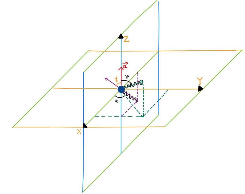
(a) Initial BHPT setup

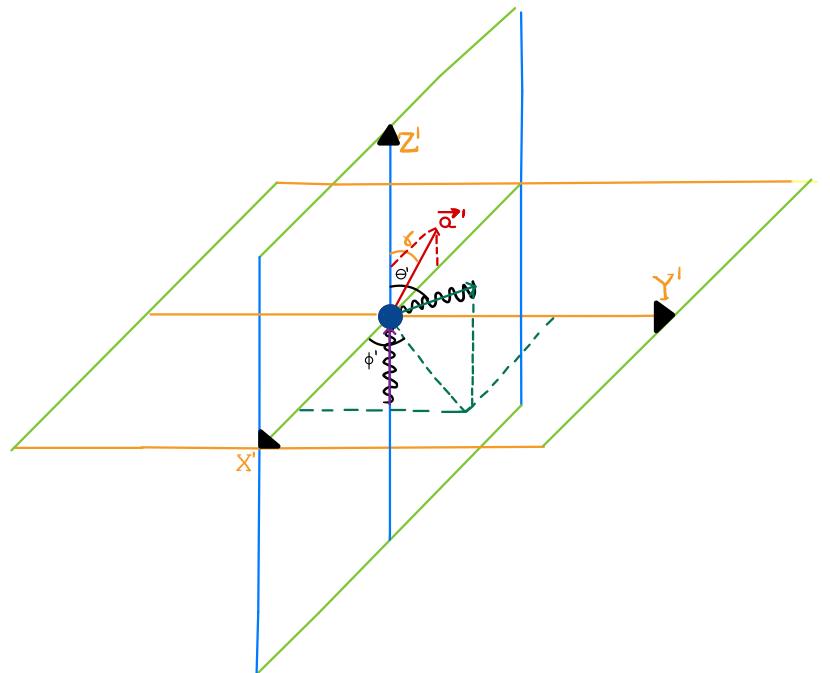
(b) Rotated BHPT setup

Figure F.1: Gravitational wave scattering in the BHPT setup. (a) An incoming PW (purple) impinges on the BH at an angle $\gamma$ with respect to the direction of the BH spin ($\vec{a}=a\hat{z}$). The outgoing scatter wave (green) moves in a general direction with angles $\vartheta$ and $\varphi$ with respect to eh $Z$ and $X$ axis respectively. (b) Rotated frame. In this frame, the incoming PW (purple) moves along the vertical axis, whereas the spin of the BH is rotated at an angle $\gamma$ with respect to $Z^{\prime}$. The outgoing scatter wave (green) now moves in the general direction $\theta^{\prime},\phi^{\prime}$ with respect to the $Z^{\prime}$ and $X^{\prime}$ axis respectively.

The setup for this part is to consider a PW incoming into the Kerr BH, and subsequently scatter into a wave (S), which can be written as the superposition between the incoming plane wave and the outgoing spherical wave. In this computation we use the conventions for the wave and black hole momenta as indicated in Figure F.1(a). For vacuum perturbations, the Teukolsky scalar (radiation scalar) ${}_{-2}\psi=\varrho^{4}\psi_{4}$, contains all the information of the radiative dynamics and will be the main objects of study in this section. Here $\varrho=\frac{1}{r-ia\cos\vartheta}$, with $r$- and $\vartheta$ the spatial coordinates of the scattering problem. The radiation scalar satisfies the homogeneous Teukolsky equation [344]

$$\left[\frac{(r^{2}+a^{2})^{2}}{\Delta}-a^{2}\sin^{2}\vartheta\right]\frac{\partial^{2}\psi}{\partial t^{2}}+\frac{4Mar}{\Delta}\frac{\partial^{2}\psi}{\partial t\partial\varphi}+\left[\frac{a^{2}}{\Delta}-\frac{1}{\sin^{2}\vartheta}\right]\frac{\partial^{2}\psi}{\partial\varphi^{2}}-\Delta^{-s}\frac{\partial}{\partial r}\left(\Delta^{s+1}\frac{\partial\psi}{\partial r}\right)$$

$$-\frac{1}{\sin\vartheta}\frac{\partial}{\partial\vartheta}\left(\sin\vartheta\frac{\partial\psi}{\partial\vartheta}\right)-2s\left[\frac{a(r-M)}{\Delta}+\frac{i\cos\vartheta}{\sin^{2}\vartheta}\right]\frac{\partial\psi}{\partial\varphi}-2s\left[\frac{M(r^{2}-a^{2})}{\Delta}-r-ia\cos\vartheta\right]\frac{\partial\psi}{\partial t}$$

$$\qquad\qquad+s(s\cot^{2}\vartheta-1)\psi=0\,,$$ (F.1)

where $s$ corresponds to the spin of the perturbation, which for gravitational wave scattering simply fixes $s=-2$. This equation is separable in the frequency domain via

$${}_{-2}\psi(t,r,\vartheta,\varphi)=\sum_{\ell m}\int d\omega e^{-i\omega t}{}_{-2}Z_{\ell m\omega}{}_{-2}R_{\ell m\omega}(r){}_{-2}S_{\ell m}(\vartheta,\varphi,a\omega).$$ (F.2)

Here, ${}_{-2}Z_{lm\omega}$ are normalization coefficients. ${}_{s}R_{\ell m\omega}(r)$ are solutions to the homogeneous radial Teukolsky equation, and ${}_{s}S_{\ell m}(\vartheta,\varphi,a\omega)$ are the spin-weighted spheroidal harmonics with respective defining equations

$$\bigg{[}\Delta^{-s}\frac{d}{dr}\left(\Delta^{s+1}\frac{d}{dr}\right)+ \frac{K^{2}-2is(r-M)K}{\Delta}+4is\omega r-{}_{s}\lambda_{lm}\bigg{]}{}_{s}R_{\ell m\omega}(r)=0\,,$$ (F.3)

and

$$\bigg{[}\frac{1}{\sin\vartheta}\frac{d}{d\vartheta}\left(\sin\vartheta\frac{d}{d\vartheta}\right)- a^{2}\omega^{2}\sin^{2}\vartheta-\frac{(m+s\cos\vartheta)^{2}}{\sin^{2}\vartheta}-2a\omega s\cos\vartheta+s+2ma\omega+{}_{s}\lambda_{lm}\bigg{]}{}_{s}S_{lm}(\vartheta,\varphi;a\omega)=0\,,$$ (F.4)

where $K=(r^{2}+a^{2})\omega-am$, and ${}_{s}\lambda_{lm}$ is the spheroidal eigenvalue. We will come back to the Teukolsky equation in a moment. Let us in the mean time provide the classical definition of the differential cross section for the gravitational wave scattering process, which will be the observable to compare with the QFT computation. It corresponds to the outward energy flux from the scattered wave (S) normalised by the energy per unit area in the incoming plane wave (PW). In Kerr spacetime, the differential cross-section for the scattering of a plane gravitational wave can be expressed in the following form

$$\frac{d\sigma}{d\Omega}=|f(\vartheta,\varphi)|^{2}+|g(\vartheta,\varphi|^{2},$$ (F.5)

where $f$ and $g$ are respectively the complex helicity preserving and helicity reversing scattering amplitudes. Using a partial wave expansion they are given by the expressions

$$f(\vartheta,\varphi) =\sum_{l=2}^{\infty}\sum_{m=-\infty}^{\infty}{}_{-2}S_{lm}(\gamma,0;a\omega){}_{-2}S_{lm}(\vartheta,\varphi;a\omega)f_{lm\omega},$$ (F.6)

$$g(\vartheta,\varphi) =\sum_{l=2}^{\infty}\sum_{m=-\infty}^{\infty}{}_{-2}S_{lm}(\gamma,0;a\omega){}_{-2}S_{lm}(\pi-\vartheta,\varphi;a\omega)g_{lm\omega}$$ (F.7)

where $\gamma$ is the angle between the incoming wave vector and the axis of rotation of the Kerr BH (see Figure F.1(a)). The amplitude modes can be obtained by

$$f_{lm\omega} =\frac{2\pi}{i\omega}\sum_{P=\pm 1}\left(e^{2i\delta^{P}_{lm}}-1\right),$$ (F.8)

$$g_{lm\omega} =\frac{2\pi}{i\omega}\sum_{P=\pm 1}P(-1)^{l+m+2}\left(e^{2i\delta^{P}_{lm}}-1\right)$$ (F.9)

where $\delta^{P}_{lm}$ are the phase shifts in a standard scattering process. These are computed by solving the radial Teukolsky equation (F.3) [84, 127]. Let us see. For our needs we will require a vacuum Teukolsky solution, typically labelled ${}_{s}R^{\rm in}_{\ell m\omega}$, which satisfies the physical boundary condition of purely ingoing waves at the horizon, namely

$${}_{-2}R^{\rm in}_{\ell m\omega}(r)=B^{\rm trans}_{\ell m\omega}\Delta^{2}e^{-i\tilde{\omega}r_{*}},\qquad r\rightarrow r_{+},$$ (F.10)

where $r_{+}=M+\sqrt{M^{2}-a^{2}}$ is the location of the outer horizon of Kerr, $\tilde{\omega}=\omega-\frac{ma}{2Mr_{+}}$, and $B^{\rm trans}_{\ell m\omega}$ is the so called transmission coefficient. Imposing this boundary condition fixes the asymptotic form at radial infinity for each $\ell,m$ mode to be

$${}_{-2}R^{\rm in}_{\ell m\omega}(r)=B^{\rm inc}_{\ell m\omega}r^{-1}e^{-i\omega r_{*}}+B^{\rm ref}_{\ell m\omega}r^{3}e^{i\omega r_{*}},\qquad r\rightarrow\infty,$$ (F.11)

where $B^{\rm inc}_{\ell m\omega}$ and $B^{\rm ref}_{\ell m\omega}$ are the incident and reflection coefficients. Solutions to the radial Teukosky equation can be written as infinite series of hypergeometric functions or confluent hypergeometric functions, depending on the required asymptotic boundary conditions [346, 347, 348, 349]. Investigation of the asymptotic behaviour of these infinite series yields expressions for the incident and reflection coefficients:

$$B^{\rm inc}_{\ell m\omega}= \omega^{-1}\left[{K}_{\nu}-ie^{-i\pi\nu}\frac{\sin\pi(\nu-s+i\epsilon)}{\sin\pi(\nu+s-i\epsilon)}{K}_{-\nu-1}\right]A_{+}^{\nu}e^{-i(\epsilon\ln\epsilon-\frac{1-\kappa}{2}\epsilon)},$$ (F.12)

$$B^{\rm ref}_{\ell m\omega}= \omega^{-1-2s}\left[{K}_{\nu}+ie^{i\pi\nu}{K}_{-\nu-1}\right]A_{-}^{\nu}e^{i(\epsilon\ln\epsilon-\frac{1-\kappa}{2}\epsilon)},$$ (F.13)

with

$$A_{+}^{\nu}=e^{-{\pi\over 2}\epsilon}e^{{\pi\over 2}i(\nu+1-s)}2^{-1+s-i\epsilon}{\Gamma(\nu+1-s+i\epsilon)\over\Gamma(\nu+1+s-i\epsilon)}\sum_{n=-\infty}^{+\infty}a_{n}^{\nu},$$ (F.14)

$$A_{-}^{\nu}=2^{-1-s+i\epsilon}e^{-{\pi\over 2}i(\nu+1+s)}e^{-{\pi\over 2}\epsilon}\sum_{n=-\infty}^{+\infty}(-1)^{n}{(\nu+1+s-i\epsilon)_{n}\over(\nu+1-s+i\epsilon)_{n}}a_{n}^{\nu},$$ (F.15)

and

$$K_{\nu}= \frac{e^{i\epsilon\kappa}(2\epsilon\kappa)^{s-\nu-r}2^{-s}i^{r}\Gamma(1-s-2i\epsilon_{+})\Gamma(r+2\nu+2)}{\Gamma(r+\nu+1-s+i\epsilon)\Gamma(r+\nu+1+i\tau)\Gamma(r+\nu+1+s+i\epsilon)}$$

$$\times\left(\sum_{n=r}^{\infty}(-1)^{n}\,\frac{\Gamma(n+r+2\nu+1)}{(n-r)!}\frac{\Gamma(n+\nu+1+s+i\epsilon)}{\Gamma(n+\nu+1-s-i\epsilon)}\frac{\Gamma(n+\nu+1+i\tau)}{\Gamma(n+\nu+1-i\tau)}\,a_{n}^{\nu}\right)$$

$$\times\left(\sum_{n=-\infty}^{r}\frac{(-1)^{n}}{(r-n)!(r+2\nu+2)_{n}}\frac{(\nu+1+s-i\epsilon)_{n}}{(\nu+1-s+i\epsilon)_{n}}a_{n}^{\nu}\right)^{-1}.$$ (F.16)

Here $r$ is a free parameter (not to be confused with the radial coordinate) we set to be $0$, $\epsilon=2GM\omega$, $\kappa=\sqrt{1-a^{\star 2}}$, $a^{\star}=\frac{a}{GM}$, $\tau=\frac{\epsilon-mq}{\kappa}$ and $\epsilon_{\pm}=\frac{\epsilon\pm\tau}{2}$. In these expressions the series coefficients $a_{n}^{\nu}$ satisfy 3 term recurrence relations and the ‘renormalised angular momentum’ $\nu$ is determined by insisting the series all converge. The phase shifts are then simply given by

$$e^{2i\delta_{\ell m}^{P}}=(-1)^{l+1}\frac{B^{\rm ref}_{lm\omega}}{B^{\rm inc}_{lm\omega}}\,.$$ (F.17)

Solving the Teukolsky equation then means to solve for $B^{\rm inc}_{\ell m\omega}$ and $B^{\rm inc}_{\ell m\omega}$, and therefore for the phase shift (F.17) which can be use to compute the scattering amplitudes modes (F.8) and (F.9). The differential cross section can be obtained by performing the infinite sums (F.6) and (F.7), which can then be replaced in (F.5), and compare to the amplitudes result (7.32). In general, solving for this infinite sums is a very non-trivial task, and we will have to engineer a method to compare to the closed form solutions from the QFT computation. We will come bakc to this in section F.2.

In general, and as mentioned above, solutions of the Teukolsky equation encapsulate all orders in perturbation theory (all orders in $G$), and all orders in the BH’s spin. In practice solving for this conditions, this can become a non trivial task, however calculating the low frequency expansions of $B^{\rm inc}_{\ell m\omega}$ and $B^{\rm inc}_{\ell m\omega}$ ultimately come down to determining low frequency expansions of $a_{n}^{\nu}$ and $\nu$. These have been extensively studied (see e.g. [349, 350]), and so we will not discuss this problem here. The relevant results will soon be available in the Black Hole Perturbation Toolkit [351]. Comparison to the QFT computation requres a further expansion of the results in powers of the BH’s. This is a simple task up to $a^{4}$ which is the order we are interested in this thesis .

F.1 Low energy expansion

The matching to the QFT computation can actually be done at the level of the scattering amplitude, which up to a phase should coincide with the BHPT result. We calculate the partial wave amplitudes in a long wavelength limit $GM\omega\ll 1$. For this, it is crucially important that $0\leq\frac{a}{GM}<1$ when constructing the long wavelength expansion, so that we can use the tools of black hole perturbation theory. When $\frac{a}{GM}>1$ the BH ceases to have an horizon and standard methods for solving the Teukolsky equation are not clearly defined. In this thesis, we will be interested to compute the partial waves up to order $a^{4}$, where the final result is independent of whether $0\leq\frac{a}{GM}<1$ or $\frac{a}{GM}>1$.

We first construct the low frequency expansion of the harmonic modes of the amplitude functions, holding $a^{\star}=\frac{a}{GM}<1$ fixed. This is essentially a two step process.

$1.$ Calculate $f_{lm\omega}$ and $g_{lm\omega}$ as a Taylor expansion in $\epsilon=2GM\omega$. This can be given order-by-order in closed form as a function of $a^{\star}$. Further, for all $l$ greater than some value $l_{\rm min}$, the solutions can also be written as a function of $l$ and $m$. $l_{\rm min}$ is determined by the order in $\epsilon$ to which one is working. For example, up to $\epsilon^{5}$ only $l=2$ differs from the closed form general $lm$ expressions. At higher orders, successively higher values of $l$ will disagree with the general forms.
$2.$ Project the spin-weighted spheroidal-harmonic representation on to a basis of spin-weighted spherical harmonics. This is fairly straightforwardly done since in a low frequency limit one can write

$${}_{-2}S_{\ell m}(\vartheta,\varphi,a\omega)=\sum_{\pm i}d^{i}_{lm}{}_{-2}Y_{\ell+i,m}(\vartheta,\varphi)(a\omega)^{i}$$ (F.18)

where the coefficients $d^{i}_{lm}$ are well known. See e.g. Appendix B of [350].

As a matter of computational complexity, this procedure is more or less independent of whether one is dealing with polar ($\gamma=0$) or non-polar ($\gamma\neq 0$) scattering; for non-polar we simply need to keep all $m$-modes.

We now give some explicit details of the calculations of $f)$. Significant detail of such a calculation, and for $g$, can also be found in [127] where the author computed the first correction in $a\omega$ for the polar ($\gamma=0$) case. We will compute up to and including $(a\omega)^{4}$ the relevant $lm$ modes. As was noted in [127], when calculating the expansion of $\frac{B^{\rm ref}_{\ell m\omega}}{B^{\rm inc}_{\ell m\omega}}$ in small $\epsilon=2GM\omega$, the complicated function $K_{\nu}$ as given above, appears only in the schematic form $1+\frac{K_{-\nu-1}}{K_{\nu}}$. Explicit computation shows that $\frac{K_{-\nu-1}}{K_{\nu}}\sim\epsilon^{2\ell-1}$. This implies for our calculation it can only be relevant for $\ell=2,3$. As we will see below this leads to a correction to the partial wave series at $a^{\star 5}$ only for $\ell=2$, which are not relevant for the present thesis .

Omitting the cumbersome intermediate expansions we arrive at the following expression for the amplitude modes

$$f_{\ell m\omega}=\frac{\Gamma(\ell-1-i\epsilon)}{\Gamma(\ell+3+i\epsilon)}\frac{\Gamma(\ell+3)}{\Gamma(\ell-1)}\beta_{\ell m\omega}$$ (F.19)

where $\beta_{\ell m\omega}$ has the form

$$\beta_{\ell m}=1+\sum_{i=2}^{\infty}\beta^{(i)}_{\ell m}\epsilon^{i}.$$ (F.20)

The $\Gamma$-function prefactors in (F.19) absorb a significant amount of complicated structure in the low frequency expansion of $f_{\ell m\omega}$, so that the $\beta^{(i)}_{\ell m}$ are relatively simple. We find explicitly that for $i\leq 5$ the $\beta^{(i)}_{\ell m}$ are polynomials in $a^{\star}$ of order $i-1$.

The downside of the $\Gamma$-function prefactors is that the projection onto spherical harmonics is contains some subtlety. Schematically, writing the low frequency expansion of the harmonics as

$${}_{s}S_{lm}(\vartheta,\varphi,a\omega) ={}_{s}Y_{lm}+{}_{s}S_{lm}^{(1)}q\epsilon+{}_{s}S_{lm}^{(2)}q^{2}\epsilon^{2}+\ldots,$$ (F.21)

$${}_{s}S_{lm}(0,0,a\omega) =N^{(0)}_{lm}+N_{lm}^{(1)}q\epsilon+N_{lm}^{(1)}q^{2}\epsilon^{2}+\ldots,$$ (F.22)

where the $N^{(i)}_{lm}$ are constants.

Both of the above expansions are available open source in the SpinWeightedSpheroidalHarmonics package of the Black hole perturbation toolkit [351]. The full amplitude function is then

$$f(\vartheta,\varphi) =\frac{1}{i\omega}\sum_{lm}\frac{\Gamma(\ell-1-i\epsilon)}{\Gamma(\ell+3+i\epsilon)}\frac{\Gamma(\ell+3)}{\Gamma(\ell-1)}\left(N^{(0)}_{lm}+N_{lm}^{(1)}a^{\star}\epsilon+N_{lm}^{(1)}a^{\star 2}\epsilon^{2}+\ldots\right)$$ (F.23)

$$\times\left({}_{s}Y_{lm}+{}_{s}S_{lm}^{(1)}a^{\star}\epsilon+{}_{s}S_{lm}^{(2)}a^{\star 2}\epsilon^{2}+\ldots\right)\left(1+\beta^{(2)}_{\ell m}\epsilon^{2}+\ldots\right)$$ (F.24)

$$=\frac{1}{i\omega}\sum_{lm}\frac{\Gamma(\ell-1-i\epsilon)}{\Gamma(\ell+3+i\epsilon)}\frac{\Gamma(\ell+3)}{\Gamma(\ell-1)}\bigg{\{}N^{(0)}_{lm}{}_{s}Y_{lm}+\big{[}N^{(0)}_{lm}{}_{s}S_{lm}^{(1)}+{}_{s}Y_{lm}N^{(1)}_{lm}\big{]}a^{\star}\epsilon$$ (F.25)

$$+\bigg{[}\beta^{(2)}_{\ell m}N^{(0)}_{lm}{}_{s}Y_{lm}+(N^{(0)}_{lm}{}_{s}S_{lm}^{(2)}+N^{(2)}_{lm}{}_{s}Y_{lm}+N^{(1)}_{lm}{}_{s}S_{lm}^{(1)})a^{\star 2}\bigg{]}\epsilon^{2}+\ldots\bigg{\}}.$$ (F.26)

We we will be investigating the large-$a^{\star}$ limit of this expression. Knowing that $\beta^{(i)}_{\ell m}$ is at most $\mathcal{O}(a^{\star(i-1))}$ in this limit, one might naively conclude that the dominant, and relevant contribution comes entirely from the cross terms of the expansions of the spheroidal harmonics. However, when we project onto the spherical harmonics, an explicit calculation reveals that

$$\sum_{lm}\frac{\Gamma(\ell-1-i\epsilon)}{\Gamma(\ell+3+i\epsilon)}\frac{\Gamma(\ell+3)}{\Gamma(\ell-1)}\int\big{[}N^{(0)}_{lm}{}_{s}S_{lm}^{(1)}+{}_{s}Y_{lm}N^{(1)}_{lm}\big{]}{}_{s}Y_{lm}^{*}d\Omega\sim\mathcal{O}(\epsilon),$$ (F.27)

$$\sum_{lm}\frac{\Gamma(\ell-1-i\epsilon)}{\Gamma(\ell+3+i\epsilon)}\frac{\Gamma(\ell+3)}{\Gamma(\ell-1)}\int(N^{(0)}_{lm}{}_{s}S_{lm}^{(2)}+N^{(2)}_{lm}{}_{s}Y_{lm}+N^{(1)}_{lm}{}_{s}S_{lm}^{(1)}){}_{s}Y_{lm}^{*}d\Omega\sim\mathcal{O}(\epsilon),$$ (F.28)

so that the pure cross terms get an ‘order bump’ in the frequency expansion upon projection to spherical harmonics. This pattern continues as far as we have checked. The end result is that the relevant terms in the large-$a^{\star}$ expansion will be these cross terms and the leading order behaviour of the $\beta^{(i)}_{\ell m}$ functions.

For the generic-$l$ contribution we find explicitly that the $\beta^{(i)}_{\ell m}$ are polynomials in $a^{\star}$. In particular $\beta^{(i)}_{\ell m}$ is an $(i-1)$th order polynomial in $a^{\star}$. Thus the highest power of $a^{\star}$ in each $\beta^{(i)}_{\ell m}$ gives the $\mathcal{O}(G)$ contribution we seek; all other terms are higher order in $G$. Focusing purely on these terms we will write

$$\beta^{G}_{\ell m}=1+\sum_{i=2}^{\infty}\beta^{G,(i)}_{\ell m}a^{\star(i-1)}\epsilon^{i}.$$ (F.29)

For example, for $m=2$ we find

$$\beta^{G,(2)}_{\ell 2} =-\frac{2i}{l(l+1)},$$ (F.30)

$$\beta^{G,(3)}_{\ell 2} =-\frac{i\left(l^{6}+3l^{5}+3l^{4}+l^{3}-80l^{2}-80l-48\right)}{2l^{3}(l+1)^{3}(2l-1)(2l+3)},$$ (F.31)

$$\beta^{G,(4)}_{\ell 2} =\frac{i\left(l^{10}+5l^{9}+3l^{8}-18l^{7}+75l^{6}+309l^{5}-151l^{4}-848l^{3}-1696l^{2}-1216l-384\right)}{(l-1)l^{5}(l+1)^{5}(l+2)(2l-1)(2l+3)},$$ (F.32)

$$\beta^{G,(5)}_{\ell 2} =\frac{i}{8(l-1)l^{7}(l+1)^{7}(l+2)(2l-3)(2l-1)^{3}(2l+3)^{3}(2l+5)}\big{(}12l^{20}+120l^{19}+263l^{18}$$

$$-1053l^{17}-20767l^{16}-126764l^{15}-122488l^{14}+1199896l^{13}+2612040l^{12}-5081558l^{11}$$

$$-22234775l^{10}-22582443l^{9}+29249651l^{8}+123462810l^{7}+142507808l^{6}+33491616l^{5}$$

$$-65123264l^{4}-63746304l^{3}-10990080l^{2}+9262080l+4147200\big{)},$$

and analogously for other harmonics.

F.2 Matching procedure: BHPT and QFT amplitudes

In order to match our QFT amplitudes with the results from BHPT it is convenient to now project the previous amplitude function (F.6) onto spin weighted spherical harmonics as in (F.18)

$$f(\vartheta,\varphi)=\sum_{lm}{}_{-2}Y_{lm}(\vartheta,\varphi)f_{lm}(\gamma),$$ (F.34)

where $f_{lm}=f^{N}+f^{(1)}_{lm}z+f^{(2)}_{lm}z^{2}+\ldots$ and $z=a^{\star}\epsilon={{\color[rgb]{0,0,0}2}}a\omega$. While there are some subtleties in the projection as discussed in Sec. 4.3.1. of [127], we will omit such details here.

An important feature emerges for polar scattering, which is obtained by setting $\gamma=0$. One finds that only the modes $f^{(i)}_{l0}$ are non-trivial and

$$f^{(i)}_{l0}(0)=0\,,\,\,\textrm{ for }\,\,i=2k+1\,\,\textrm{ or for }i\leq l.$$ (F.35)

This means that, other than the Newtonian term, for polar scattering the infinite sum over the spherical harmonics reduces to a finite sum for each power of $z$. This has been noted in [127] for the case of GW scattering in Kerr.

In the off-axis case where $\gamma\neq 0$, no such simplification occurs, and we find it convenient to compare with the 4-pt amplitudes (7.26) , by working mode-by-mode. To do this we first need to align our coordinates by a rotation.

Let us see how this works. The amplitude function (F.34) is written as a sum over the spin weighted spherical harmonics ${}_{-2}Y_{lm}(\vartheta,\varphi)$, where $(\vartheta,\varphi)$ is the direction of the outgoing wave in a coordinate system where the spin direction is $\vartheta=0$, i.e. the $+Z$ direction, and the incoming wave is in the direction $(\vartheta,\varphi)=(\gamma,0)$ (in the $X$-$Z$ plane), so that $\gamma$ is the angle between the spin and the incoming wave.

Now let us rotate our $(\vartheta,\varphi)$–$(X,Y,Z)$ coordinate system about the $Y$ axis (the same as the new $Y^{\prime}$-axis) by an angle $\gamma$, to bring the incoming wave direction to the new $+Z^{\prime}$ direction, and call the new coordinates $(\theta^{\prime},\phi^{\prime})$–$(X^{\prime},Y^{\prime},Z^{\prime})$ (see Figure F.1(b)). This is still not the same as the $(\theta,\phi)$–$(x,y,z)$ coordinate system used in eq. 7.26, but now the $z$-axes are the same. The rotation of the spin weighted spherical harmonics is known to be accomplished by

$${}_{-2}Y_{lm}(\theta^{\prime},\phi^{\prime})=\sum_{m^{\prime}}D^{l*}_{mm^{\prime}}(\gamma)\;{}_{-2}Y_{lm^{\prime}}(\vartheta,\varphi)\,,$$ (F.36)

where $D^{l*}_{mm^{\prime}}$ is the (complex conjugate) Wigner $D$-matrix with Euler angles $(0,\gamma,0)$,

$$D^{l*}_{mm^{\prime}}(\gamma)=D^{l*}_{mm^{\prime}}(0,\gamma,0)=(-1)^{m^{\prime}}\sqrt{\frac{4\pi}{2l+1}}{}_{-m^{\prime}}Y_{lm}(\gamma,0).$$ (F.37)

Now the amplitude (F.34) takes the form

$$f=\sum_{lm}{}_{-2}Y_{lm}(\theta^{\prime},\phi^{\prime})f^{\prime}_{lm}(\gamma),$$ (F.38)

with

$$\boxed{f^{\prime}_{lm}(\gamma)=\sum_{m^{\prime}}D^{l*}_{m^{\prime}m}(\gamma)\;f_{lm^{\prime}}(\gamma)}\,,$$ (F.39)

where we relabeled $m\leftrightarrow m^{\prime}$ after substituting. Now, in this new $(\theta^{\prime},\phi^{\prime})$ coordinate system, with corresponding $(X^{\prime},Y^{\prime},Z^{\prime})$, the spin vector is $\vec{a}=a(-\sin\gamma,0,\cos\gamma)$, the incoming wave vector is $\vec{k}_{2}=(0,0,\omega)$, and the outgoing wave vector is $\vec{k}_{3}=\omega(\sin\theta^{\prime}\cos\phi^{\prime},\sin\theta^{\prime}\sin\phi^{\prime},\cos\theta^{\prime})$.

Finally, we have the third $(\theta,\phi)$–$(x,y,z)$ coordinate system used in (7.26), where $\vec{k}_{2}$ is in the $z$ direction (same as $Z^{\prime}$ direction) and $\vec{k}_{3}$ is in the $x$-$z$ plane at an angle $\theta$ from $\vec{k}_{2}$, and this is the same $\theta=\theta^{\prime}$ from the second coordinates. To translate the result (7.26) into the $(\theta^{\prime},\phi^{\prime})$ coordinates, we use $\theta=\theta^{\prime}$ and do a rotation by an angle of $\phi^{\prime}$ around the $x$-axis. This simply amounts to take

$$a_{z}=a\cos\gamma,\quad a_{x}=-a\sin\gamma\cos\phi^{\prime},\quad a_{y}=-a\sin\gamma\sin\phi^{\prime},$$ (F.40)

as can be confirmed by comparing the values of $\vec{a}\cdot\vec{k}_{2}$, $\vec{a}\cdot\vec{k}_{3}$ and $\vec{k}_{2}\cdot\vec{k}_{3}$.

It is most convenient to compare our amplitudes results from (7.26) using $(\theta,\phi)$ to our BHPT results using $(\vartheta,\varphi)$ by comparing the amplitudes of their spin weighted spherical harmonic modes in the intermediate $(\theta^{\prime},\phi^{\prime})$ coordinates as in (F.38).

We recall that the amplitude function $f$ at the leading order in $\epsilon$ (at fixed $a\omega=a^{\star}\epsilon/2$), coming from the tree-level scattering amplitude (7.26), is

$$f=\frac{\kappa^{2}M^{2}\cos^{4}(\theta/2)}{4\sin^{2}(\theta/2)}\big{[}1+\mathcal{F}(\omega,a,\theta)+\frac{1}{2!}\mathcal{F}(\omega,a,\theta)^{2}+\frac{1}{3!}\mathcal{F}(\omega,a,\theta)^{3}+\frac{1}{4!}\mathcal{F}(\omega,a,\theta)^{4}\big{]}$$ (F.41)

which is expressed in terms of $(\theta^{\prime},\phi^{\prime})$ by using $\theta=\theta^{\prime}$ and (F.40). Its mode amplitudes $f^{\prime}_{lm}$ from (F.38) are given by integrals over the 2-sphere,

$$\boxed{f^{\prime}_{lm}(\gamma)=\int d\Omega^{\prime}\,{}_{-2}Y^{*}_{lm}(\theta^{\prime},\phi^{\prime})f(\gamma,\theta^{\prime},\phi^{\prime})}\,,$$ (F.42)

and depend only on the angle $\gamma$ between the incoming momentum and the spin, and on the parameters $\epsilon$ and $a^{\star}$. Then, matching of the BHPT results to the QFT results translates to show (F.42) and (F.39) agree for all $\ell,m$.

In general, let us write these as an expansion in $\epsilon$, focusing on the leading order in the large $a^{\star}$ expansion at each order in $\epsilon$,

$$f^{\prime}_{lm}=\sum_{n=0}^{\infty}\epsilon^{n}\Big{[}f^{\prime}_{lm,n}a^{\star}{}^{n}+\mathcal{O}(a^{\star}{}^{(n-1)})\Big{]}.$$ (F.43)

We find that this pattern also holds for the analytically continued BHPT amplitudes in the large $a^{\star}$ expansion for the orders considered here, i.e. up to $a^{4}$.

At linear order in spin, from (F.41), we find

$$\begin{aligned} f^{\prime}_{00,1}&=0,\\ \{f^{\prime}_{1m,1}\}&=\{0,0,0\},\\ \{f^{\prime}_{2m,1}\}&=\sqrt{\frac{\pi}{5}}\{0,0,0,3\sin\gamma,-2\cos\gamma\},\\ \{f^{\prime}_{3m,1}\}&=\sin\gamma\{0,0,0,0,\sqrt{\frac{7\pi}{10}},0,\sqrt{\frac{7\pi}{6}}\},\end{aligned}$$ (F.44)

and so on, with $m=\{-l,\ldots,l\}$. From (F.41) at quadratic order in spin, we find

$$\begin{aligned} f^{\prime}_{00,2}&=0,\\ \{f^{\prime}_{1m,2}\}&=\{0,0,0\},\\ \{f^{\prime}_{2m,2}\}&=\{0,0,\frac{1}{4}\sqrt{\frac{5\pi}{6}}\sin^{2}\gamma,-\frac{2}{3}\sqrt{\frac{\pi}{5}}\cos\gamma\sin\gamma,\frac{1}{24}\sqrt{\frac{\pi}{5}}(9\cos(2\gamma)-5)\},\\ \{f^{\prime}_{3m,2}\}&=\{0,0,0,\frac{1}{4}\sqrt{\frac{3\pi}{70}}\sin^{2}\gamma,\frac{1}{6}\sqrt{\frac{\pi}{70}}\sin(2\gamma),-\frac{1}{24}\sqrt{\frac{\pi}{7}}(3\cos(2\gamma)+1),-\sqrt{\frac{\pi}{42}}\sin\gamma\cos\gamma\},\\ \{f^{\prime}_{4m,2}\}&=\sin^{2}\gamma\{0,0,0,0,\frac{1}{8}\sqrt{\frac{\pi}{10}},0,0,0,\frac{3}{16}\sqrt{\frac{\pi}{7}}\},\end{aligned}$$ (F.45)

and so on. At cubic order in spin, it follows

$$\begin{aligned} f^{\prime}_{00,3}&=0,\\ \{f^{\prime}_{1m,3}\}&=\{0,0,0\},\\ \{f^{\prime}_{2m,3}\}&=\{0,\frac{5}{168}\sqrt{5\pi}\sin^{3}\gamma,-\frac{2}{7}\sqrt{\frac{2\pi}{15}}\cos\gamma\sin^{2}\gamma,\frac{1}{336}\sqrt{\frac{\pi}{5}}(1+39\cos 2\gamma)\sin\gamma,\\ &\qquad\qquad\frac{1}{504}\sqrt{\frac{\pi}{5}}\cos\gamma(23-31\cos 2\gamma)\},\\ \{f^{\prime}_{3m,3}\}&=\{0,0,-\frac{1}{96}\sqrt{\frac{\pi}{70}}\sin^{3}\gamma,\frac{1}{8}\sqrt{\frac{3\pi}{70}}\cos\gamma\sin^{2}\gamma,-\frac{1}{192}\sqrt{\frac{\pi}{70}}(17+39\cos 2\gamma)\sin\gamma,\\ &\qquad\qquad\frac{1}{144}\sqrt{\frac{\pi}{7}}(11\cos 2\gamma-7)\cos\gamma,\frac{1}{64}\sqrt{\frac{\pi}{42}}(9\cos 2\gamma-1)\sin\gamma\},\end{aligned}$$ (F.46)

and so on. Finally, at quartic order in spin we have

$$\begin{aligned} f^{\prime}_{00,4}&=0,\\ \{f^{\prime}_{1m,4}\}&=\{0,0,0\},\\ \{f^{\prime}_{2m,4}\}&=\{\frac{769}{10752}\sqrt{\frac{\pi}{5}}\sin^{4}\gamma,-\frac{67}{672}\sqrt{\frac{\pi}{5}}\cos\gamma\sin^{3}\gamma,\frac{1}{896}\sqrt{\frac{\pi}{30}}(37+103\cos 2\gamma)\sin^{2}\gamma,\\ &\qquad\qquad\frac{1}{2688}\sqrt{\frac{\pi}{5}}(17-41\cos 2\gamma)\sin 2\gamma,\frac{1}{43008}\sqrt{\frac{\pi}{5}}(77-156\cos 2\gamma+143\cos 4\gamma)\},\\ \{f^{\prime}_{3m,4}\}&=\{0,-\frac{233}{23040}\sqrt{\frac{\pi}{7}}\sin^{4}\gamma,\frac{1}{9}\sqrt{\frac{\pi}{70}}\cos\gamma\sin^{3}\gamma,-\frac{1}{1152}\sqrt{\frac{\pi}{210}}(97+179\cos 2\gamma)\sin^{2}\gamma,\\ &\qquad\frac{1}{144}\sqrt{\frac{\pi}{70}}(7\cos 2\gamma-2)\sin 2\gamma,-\frac{1}{18432}\sqrt{\frac{\pi}{7}}(33-76\cos 2\gamma+107\cos 4\gamma),\frac{1}{144}\sqrt{\frac{\pi}{42}}(\sin 2\gamma-\sin 4\gamma)\},\end{aligned}$$ (F.47)

and so on. Remarkably, also continuing to large values of $l$, we find that all of these $(\epsilon a^{\star})^{i},$ for $i=1,2,3,4$ terms in the mode amplitudes from the (minimal) tree-level scattering amplitude (F.41) precisely match those computed from the analytically continued BHPT theory amplitudes as described above. Amplitude (F.41) in turn provides a closed form for the infinite partial waves from BHPT. An analogous mode expansion can be made for the amplitude (7.28) and show it agrees with the BHPT computation up to quartic order in spin.

References

- [1] Z. Bern, J.P. Gatica, E. Herrmann, A. Luna and M. Zeng, Scalar QED as a toy model for higher-order effects in classical gravitational scattering, 2112.12243.
- [2] LIGO Scientific Collaboration and Virgo Collaboration collaboration, Observation of gravitational waves from a binary black hole merger, Phys. Rev. Lett. 116 (2016) 061102.
- [3] A. Buonanno and B.S. Sathyaprakash, Sources of Gravitational Waves: Theory and Observations, (2014) [1410.7832].
- [4] A. Buonanno, M. Khalil, D. O’Connell, R. Roiban, M.P. Solon and M. Zeng, Snowmass White Paper: Gravitational Waves and Scattering Amplitudes, in 2022 Snowmass Summer Study, 4, 2022 [2204.05194].
- [5] Z. Bern, J.J. Carrasco, M. Chiodaroli, H. Johansson and R. Roiban, The SAGEX Review on Scattering Amplitudes, Chapter 2: An Invitation to Color-Kinematics Duality and the Double Copy, 2203.13013.
- [6] A. Luna, I. Nicholson, D. O’Connell and C.D. White, Inelastic Black Hole Scattering from Charged Scalar Amplitudes, JHEP 03 (2018) 044 [1711.03901].
- [7] F. Cachazo and A. Guevara, Leading Singularities and Classical Gravitational Scattering, JHEP 02 (2020) 181 [1705.10262].
- [8] A. Einstein, Über Gravitationswellen, Sitzungsberichte der Königlich Preußischen Akademie der Wissenschaften (Berlin (1918) 154.
- [9] LIGO Scientific, Virgo collaboration, Observation of Gravitational Waves from a Binary Black Hole Merger, Phys. Rev. Lett. 116 (2016) 061102 [1602.03837].
- [10] S. Mastrogiovanni, D. Steer and M. Barsuglia, Probing modified gravity theories and cosmology using gravitational-waves and associated electromagnetic counterparts, Physical Review D 102 (2020) .
- [11] H.S. Chia, Probing Particle Physics with Gravitational Waves, Ph.D. thesis, Amsterdam U., 2020. 2012.09167.
- [12] B. Abbott, R. Abbott, T. Abbott, F. Acernese, K. Ackley, C. Adams et al., Gw170817: Observation of gravitational waves from a binary neutron star inspiral, Physical Review Letters 119 (2017) .
- [13] R. Abbott, T.D. Abbott, S. Abraham, F. Acernese, K. Ackley, A. Adams et al., Observation of gravitational waves from two neutron star–black hole coalescences, The Astrophysical Journal Letters 915 (2021) L5.
- [14] LIGO Scientific collaboration, Gravitational wave astronomy with LIGO and similar detectors in the next decade, 1904.03187.
- [15] M. Favata, The gravitational-wave memory effect, Class. Quant. Grav. 27 (2010) 084036 [1003.3486].
- [16] KAGRA collaboration, KAGRA: 2.5 Generation Interferometric Gravitational Wave Detector, Nature Astron. 3 (2019) 35 [1811.08079].
- [17] M. Saleem et al., The science case for LIGO-India, Class. Quant. Grav. 39 (2022) 025004 [2105.01716].
- [18] M. Maggiore et al., Science Case for the Einstein Telescope, JCAP 03 (2020) 050 [1912.02622].
- [19] D. Reitze et al., Cosmic Explorer: The U.S. Contribution to Gravitational-Wave Astronomy beyond LIGO, Bull. Am. Astron. Soc. 51 (2019) 035 [1907.04833].
- [20] F. Pretorius, Evolution of binary black hole spacetimes, Phys. Rev. Lett. 95 (2005) 121101 [gr-qc/0507014].
- [21] S.A. Teukolsky, Perturbations of a Rotating Black Hole. I. Fundamental Equations for Gravitational, Electromagnetic, and Neutrino-Field Perturbations, Apj 185 (1973) 635.
- [22] K.D. Kokkotas and B.G. Schmidt, Quasinormal modes of stars and black holes, Living Rev. Rel. 2 (1999) 2 [gr-qc/9909058].
- [23] L. Blanchet, Gravitational Radiation from Post-Newtonian Sources and Inspiralling Compact Binaries, Living Rev. Rel. 17 (2014) 2 [1310.1528].
- [24] T. Futamase and Y. Itoh, The post-Newtonian approximation for relativistic compact binaries, Living Rev. Rel. 10 (2007) 2.
- [25] A. Buonanno and T. Damour, Effective one-body approach to general relativistic two-body dynamics, Phys. Rev. D 59 (1999) 084006.
- [26] A. Buonanno and T. Damour, Transition from inspiral to plunge in binary black hole coalescences, Phys. Rev. D62 (2000) 064015 [gr-qc/0001013].
- [27] L. Santamaria et al., Matching post-Newtonian and numerical relativity waveforms: systematic errors and a new phenomenological model for non-precessing black hole binaries, Phys. Rev. D 82 (2010) 064016 [1005.3306].
- [28] T. Damour and A. Nagar, The effective one-body description of the two-body problem, in Mass and Motion in General Relativity, L. Blanchet, A. Spallicci and B. Whiting, eds., (Dordrecht), pp. 211–252, Springer Netherlands (2011), DOI.
- [29] T. Damour, Gravitational scattering, post-minkowskian approximation, and effective-one-body theory, Physical Review D 94 (2016) .
- [30] R.A. Porto, The effective field theorist’s approach to gravitational dynamics, Phys. Rept. 633 (2016) 1 [1601.04914].
- [31] W.D. Goldberger and A.K. Ridgway, Bound states and the classical double copy, Phys. Rev. D 97 (2018) 085019 [1711.09493].
- [32] W.D. Goldberger, J. Li and S.G. Prabhu, Spinning particles, axion radiation, and the classical double copy, Phys. Rev. D97 (2018) 105018 [1712.09250].
- [33] J. Vines, J. Steinhoff and A. Buonanno, Spinning-black-hole scattering and the test-black-hole limit at second post-Minkowskian order, Phys. Rev. D 99 (2019) 064054 [1812.00956].
- [34] T. Damour, Classical and quantum scattering in post-Minkowskian gravity, Phys. Rev. D 102 (2020) 024060 [1912.02139].
- [35] T. Damour, Radiative contribution to classical gravitational scattering at the third order in , Phys. Rev. D 102 (2020) 124008 [2010.01641].
- [36] G. Kälin and R.A. Porto, From Boundary Data to Bound States, JHEP 01 (2020) 072 [1910.03008].
- [37] G. Kälin and R.A. Porto, From boundary data to bound states. Part II. Scattering angle to dynamical invariants (with twist), JHEP 02 (2020) 120 [1911.09130].
- [38] G. Kälin and R.A. Porto, Post-Minkowskian Effective Field Theory for Conservative Binary Dynamics, JHEP 11 (2020) 106 [2006.01184].
- [39] G. Kälin, Z. Liu and R.A. Porto, Conservative Dynamics of Binary Systems to Third Post-Minkowskian Order from the Effective Field Theory Approach, Phys. Rev. Lett. 125 (2020) 261103 [2007.04977].
- [40] W.D. Goldberger, J. Li and I.Z. Rothstein, Non-conservative effects on spinning black holes from world-line effective field theory, JHEP 06 (2021) 053 [2012.14869].
- [41] A. Brandhuber, G. Chen, G. Travaglini and C. Wen, A new gauge-invariant double copy for heavy-mass effective theory, JHEP 07 (2021) 047 [2104.11206].
- [42] A. Brandhuber, G. Chen, G. Travaglini and C. Wen, Classical gravitational scattering from a gauge-invariant double copy, JHEP 10 (2021) 118 [2108.04216].
- [43] C. Cheung and M.P. Solon, Classical gravitational scattering at (G3) from Feynman diagrams, JHEP 06 (2020) 144 [2003.08351].
- [44] C. Cheung, I.Z. Rothstein and M.P. Solon, From Scattering Amplitudes to Classical Potentials in the Post-Minkowskian Expansion, Phys. Rev. Lett. 121 (2018) 251101 [1808.02489].
- [45] Z. Bern, C. Cheung, R. Roiban, C.-H. Shen, M.P. Solon and M. Zeng, Scattering Amplitudes and the Conservative Hamiltonian for Binary Systems at Third Post-Minkowskian Order, Phys. Rev. Lett. 122 (2019) 201603 [1901.04424].
- [46] Z. Bern, C. Cheung, R. Roiban, C.-H. Shen, M.P. Solon and M. Zeng, Black Hole Binary Dynamics from the Double Copy and Effective Theory, JHEP 10 (2019) 206 [1908.01493].
- [47] Z. Bern, J. Parra-Martinez, R. Roiban, M.S. Ruf, C.-H. Shen, M.P. Solon et al., Scattering Amplitudes and Conservative Binary Dynamics at , Phys. Rev. Lett. 126 (2021) 171601 [2101.07254].
- [48] N.E.J. Bjerrum-Bohr, P.H. Damgaard, G. Festuccia, L. Planté and P. Vanhove, General Relativity from Scattering Amplitudes, Phys. Rev. Lett. 121 (2018) 171601 [1806.04920].
- [49] A. Cristofoli, N.E.J. Bjerrum-Bohr, P.H. Damgaard and P. Vanhove, Post-Minkowskian Hamiltonians in general relativity, Phys. Rev. D 100 (2019) 084040 [1906.01579].
- [50] N.E.J. Bjerrum-Bohr, A. Cristofoli and P.H. Damgaard, Post-Minkowskian Scattering Angle in Einstein Gravity, JHEP 08 (2020) 038 [1910.09366].
- [51] N.E.J. Bjerrum-Bohr, P.H. Damgaard, L. Planté and P. Vanhove, Classical Gravity from Loop Amplitudes, 2104.04510.
- [52] P. Di Vecchia, C. Heissenberg, R. Russo and G. Veneziano, Universality of ultra-relativistic gravitational scattering, Phys. Lett. B 811 (2020) 135924 [2008.12743].
- [53] P. Di Vecchia, C. Heissenberg, R. Russo and G. Veneziano, Radiation Reaction from Soft Theorems, Phys. Lett. B 818 (2021) 136379 [2101.05772].
- [54] Z. Bern, A. Luna, R. Roiban, C.-H. Shen and M. Zeng, Spinning black hole binary dynamics, scattering amplitudes, and effective field theory, Phys. Rev. D 104 (2021) 065014 [2005.03071].
- [55] M.-Z. Chung, Y.-T. Huang and J.-W. Kim, Classical potential for general spinning bodies, JHEP 09 (2020) 074 [1908.08463].
- [56] M.-Z. Chung, Y.-t. Huang, J.-W. Kim and S. Lee, Complete Hamiltonian for spinning binary systems at first post-Minkowskian order, JHEP 05 (2020) 105 [2003.06600].
- [57] A. Guevara, Holomorphic Classical Limit for Spin Effects in Gravitational and Electromagnetic Scattering, JHEP 04 (2019) 033 [1706.02314].
- [58] A. Guevara, A. Ochirov and J. Vines, Scattering of Spinning Black Holes from Exponentiated Soft Factors, JHEP 09 (2019) 056 [1812.06895].
- [59] A. Guevara, A. Ochirov and J. Vines, Black-hole scattering with general spin directions from minimal-coupling amplitudes, Phys. Rev. D 100 (2019) 104024 [1906.10071].
- [60] R. Aoude, K. Haddad and A. Helset, On-shell heavy particle effective theories, JHEP 05 (2020) 051 [2001.09164].
- [61] Y.F. Bautista and A. Guevara, On the double copy for spinning matter, JHEP 11 (2021) 184 [1908.11349].
- [62] J. Blümlein, A. Maier, P. Marquard and G. Schäfer, The fifth-order post-Newtonian Hamiltonian dynamics of two-body systems from an effective field theory approach: potential contributions, Nucl. Phys. B 965 (2021) 115352 [2010.13672].
- [63] J. Blümlein, A. Maier, P. Marquard and G. Schäfer, Testing binary dynamics in gravity at the sixth post-Newtonian level, Phys. Lett. B 807 (2020) 135496 [2003.07145].
- [64] D. Bini, T. Damour and A. Geralico, Novel approach to binary dynamics: application to the fifth post-Newtonian level, Phys. Rev. Lett. 123 (2019) 231104 [1909.02375].
- [65] Z. Bern, J. Parra-Martinez, R. Roiban, E. Sawyer and C.-H. Shen, Leading Nonlinear Tidal Effects and Scattering Amplitudes, JHEP 05 (2021) 188 [2010.08559].
- [66] H. Kawai, D.C. Lewellen and S.-H.H. Tye, A relation between tree amplitudes of closed and open strings, Nuclear Physics B 269 (1986) 1.
- [67] Z. Bern, J. Carrasco and H. Johansson, New Relations for Gauge-Theory Amplitudes, Phys. Rev. D 78 (2008) 085011 [0805.3993].
- [68] N. Arkani-Hamed, T.-C. Huang and Y.-t. Huang, Scattering Amplitudes For All Masses and Spins, 1709.04891.
- [69] K. Chetyrkin and F. Tkachov, Integration by parts: The algorithm to calculate beta-functions in 4 loops, Nuclear Physics B 192 (1981) 159.
- [70] F. Tkachov, A theorem on analytical calculability of 4-loop renormalization group functions, Physics Letters B 100 (1981) 65.
- [71] A. Kotikov, Differential equations method. new technique for massive feynman diagram calculation, Physics Letters B 254 (1991) 158.
- [72] Z. Bern, L.J. Dixon and D.A. Kosower, Dimensionally regulated one loop integrals, Phys. Lett. B 302 (1993) 299 [hep-ph/9212308].
- [73] T. Gehrmann and E. Remiddi, Differential equations for two-loop four-point functions, Nuclear Physics B 580 (2000) 485–518.
- [74] J.M. Henn, Multiloop integrals in dimensional regularization made simple, Phys. Rev. Lett. 110 (2013) 251601 [1304.1806].
- [75] J.M. Henn, Lectures on differential equations for Feynman integrals, J. Phys. A 48 (2015) 153001 [1412.2296].
- [76] M.V.S. Saketh, J. Vines, J. Steinhoff and A. Buonanno, Conservative and radiative dynamics in classical relativistic scattering and bound systems, 2109.05994.
- [77] P. Di Vecchia, C. Heissenberg, R. Russo and G. Veneziano, The eikonal approach to gravitational scattering and radiation at (G3), JHEP 07 (2021) 169 [2104.03256].
- [78] D.A. Kosower, B. Maybee and D. O’Connell, Amplitudes, Observables, and Classical Scattering, JHEP 02 (2019) 137 [1811.10950].
- [79] R. Aoude, K. Haddad and A. Helset, Tidal effects for spinning particles, JHEP 03 (2021) 097 [2012.05256].
- [80] W.D. Goldberger and A.K. Ridgway, Radiation and the classical double copy for color charges, Phys. Rev. D 95 (2017) 125010 [1611.03493].
- [81] J. Vines, Scattering of two spinning black holes in post-Minkowskian gravity, to all orders in spin, and effective-one-body mappings, 1709.06016.
- [82] W.D. Goldberger and I.Z. Rothstein, An Effective Field Theory of Quantum Mechanical Black Hole Horizons, JHEP 04 (2020) 056 [1912.13435].
- [83] W.D. Goldberger and I.Z. Rothstein, Virtual Hawking Radiation, Phys. Rev. Lett. 125 (2020) 211301 [2007.00726].
- [84] Y.F. Bautista, A. Guevara, C. Kavanagh and J. Vines, From Scattering in Black Hole Backgrounds to Higher-Spin Amplitudes: Part I, 2107.10179.
- [85] Y.F. Bautista, A. Guevara, C. Kavanagh and J. Vines, From Scattering in Black Hole Backgrounds to Higher-Spin Amplitudes: Part II, in preparation, .
- [86] Z. Bern, J. Parra-Martinez, R. Roiban, M.S. Ruf, C.-H. Shen, M.P. Solon et al., Scattering Amplitudes, the Tail Effect, and Conservative Binary Dynamics at , 2112.10750.
- [87] C. Dlapa, G. Kälin, Z. Liu and R.A. Porto, Conservative Dynamics of Binary Systems at Fourth Post-Minkowskian Order in the Large-eccentricity Expansion, 2112.11296.
- [88] W.-M. Chen, M.-Z. Chung, Y.-t. Huang and J.-W. Kim, The 2PM Hamiltonian for binary Kerr to quartic in spin, 2111.13639.
- [89] G.U. Jakobsen and G. Mogull, Conservative and radiative dynamics of spinning bodies at third post-Minkowskian order using worldline quantum field theory, 2201.07778.
- [90] Z. Bern, D. Kosmopoulos, A. Luna, R. Roiban and F. Teng, Binary Dynamics Through the Fifth Power of Spin at , 2203.06202.
- [91] R. Aoude, K. Haddad and A. Helset, Searching for Kerr in the 2PM amplitude, 2203.06197.
- [92] E. Herrmann, J. Parra-Martinez, M.S. Ruf and M. Zeng, Radiative classical gravitational observables at (G3) from scattering amplitudes, JHEP 10 (2021) 148 [2104.03957].
- [93] E. Herrmann, J. Parra-Martinez, M.S. Ruf and M. Zeng, Gravitational Bremsstrahlung from Reverse Unitarity, Phys. Rev. Lett. 126 (2021) 201602 [2101.07255].
- [94] A.V. Manohar, A.K. Ridgway and C.-H. Shen, Radiated Angular Momentum and Dissipative Effects in Classical Scattering, 2203.04283.
- [95] M. Khalil, A. Buonanno, J. Steinhoff and J. Vines, Radiation-reaction force and multipolar waveforms for eccentric, spin-aligned binaries in the effective-one-body formalism, Phys. Rev. D 104 (2021) 024046 [2104.11705].
- [96] D. Bini and T. Damour, Gravitational radiation reaction along general orbits in the effective one-body formalism, Phys. Rev. D 86 (2012) 124012 [1210.2834].
- [97] G. Cho, G. Kälin and R.A. Porto, From Boundary Data to Bound States III: Radiative Effects, 2112.03976.
- [98] K.S. Thorne, Multipole expansions of gravitational radiation, Rev. Mod. Phys. 52 (1980) 299.
- [99] L. Blanchet and G. Schafer, Gravitational wave tails and binary star systems, Classical and Quantum Gravity 10 (1993) 2699.
- [100] M. Khalil, Gravitational spin-orbit dynamics at the fifth-and-a-half post-Newtonian order, Phys. Rev. D 104 (2021) 124015 [2110.12813].
- [101] Y.F. Bautista and N. Siemonsen, Post-Newtonian waveforms from spinning scattering amplitudes, JHEP 01 (2022) 006 [2110.12537].
- [102] Y.F. Bautista and A. Guevara, From Scattering Amplitudes to Classical Physics: Universality, Double Copy and Soft Theorems, 1903.12419.
- [103] M.-Z. Chung, Y.-T. Huang, J.-W. Kim and S. Lee, The simplest massive S-matrix: from minimal coupling to Black Holes, JHEP 04 (2019) 156 [1812.08752].
- [104] N. Arkani-Hamed, Y.-t. Huang and D. O’Connell, Kerr Black Holes as Elementary Particles, 1906.10100.
- [105] J.D. Jackson, Classical electrodynamics; 2nd ed., Wiley, New York, NY (1975).
- [106] Y.F. Bautista and A. Laddha, Soft Constraints on KMOC Formalism, 2111.11642.
- [107] A. Manu, D. Ghosh, A. Laddha and P.V. Athira, Soft radiation from scattering amplitudes revisited, JHEP 05 (2021) 056 [2007.02077].
- [108] D. Christodoulou, Nonlinear nature of gravitation and gravitational-wave experiments, Phys. Rev. Lett. 67 (1991) 1486.
- [109] Y.F. Bautista, A. Laddha and Y. Zhang, Log soft theorems from KMOC formalism, in preparation, .
- [110] V.B. Braginsky and K.S. Thorne, Gravitational-wave bursts with memory and experimental prospects, Nature 327 (1987) 123.
- [111] P. Di Vecchia, C. Heissenberg and R. Russo, Angular momentum of zero-frequency gravitons, 2203.11915.
- [112] P. Di Vecchia, C. Heissenberg, R. Russo and G. Veneziano, The eikonal operator at arbitrary velocities I: the soft-radiation limit, 2204.02378.
- [113] D. Gerosa, M. Kesden, E. Berti, R. O’Shaughnessy and U. Sperhake, Resonant-plane locking and spin alignment in stellar-mass black-hole binaries: a diagnostic of compact-binary formation, Phys. Rev. D 87 (2013) 104028 [1302.4442].
- [114] S. Vitale, R. Lynch, R. Sturani and P. Graff, Use of gravitational waves to probe the formation channels of compact binaries, Class. Quant. Grav. 34 (2017) 03LT01 [1503.04307].
- [115] S. Biscoveanu, M. Isi, V. Varma and S. Vitale, Measuring the spins of heavy binary black holes, Phys. Rev. D 104 (2021) 103018 [2106.06492].
- [116] O. Burke, J.R. Gair, J. Simón and M.C. Edwards, Constraining the spin parameter of near-extremal black holes using LISA, Phys. Rev. D 102 (2020) 124054 [2010.05932].
- [117] J. Li and S.G. Prabhu, Gravitational radiation from the classical spinning double copy, Phys. Rev. D 97 (2018) 105019 [1803.02405].
- [118] B.M. Barker and R.F. O’Connell, Gravitational Two-Body Problem with Arbitrary Masses, Spins, and Quadrupole Moments, Phys. Rev. D12 (1975) 329.
- [119] B.M. Barker and R.F. O’Connell, The gravitational interaction: Spin, rotation, and quantum effects-a review, General Relativity and Gravitation 11 (1979) 149.
- [120] G.U. Jakobsen, G. Mogull, J. Plefka and J. Steinhoff, Gravitational Bremsstrahlung and Hidden Supersymmetry of Spinning Bodies, 2106.10256.
- [121] N.D. Hari Dass and V. Soni, Feynman Graph Derivation of Einstein Quadrupole Formula, J. Phys. A 15 (1982) 473.
- [122] K.S. Thorne, Multipole Expansions of Gravitational Radiation, Rev. Mod. Phys. 52 (1980) 299.
- [123] L. Blanchet and T. Damour, Radiative gravitational fields in general relativity I. general structure of the field outside the source, Phil. Trans. Roy. Soc. Lond. A320 (1986) 379.
- [124] L. Blanchet, T. Damour and B.R. Iyer, Gravitational waves from inspiralling compact binaries: Energy loss and wave form to second postNewtonian order, Phys. Rev. D 51 (1995) 5360 [gr-qc/9501029].
- [125] L. Blanchet, On the multipole expansion of the gravitational field, Class. Quant. Grav. 15 (1998) 1971 [gr-qc/9801101].
- [126] H. Johansson and A. Ochirov, Double copy for massive quantum particles with spin, 1906.12292.
- [127] S.R. Dolan, Scattering and Absorption of Gravitational Plane Waves by Rotating Black Holes, Class. Quant. Grav. 25 (2008) 235002 [0801.3805].
- [128] E. Guadagnini, Gravitons scattering from classical matter, Class. Quant. Grav. 25 (2008) 095012 [0803.2855].
- [129] A. Barbieri and E. Guadagnini, Gravitational helicity interaction, Nucl. Phys. B 719 (2005) 53 [gr-qc/0504078].
- [130] B. Maybee, D. O’Connell and J. Vines, Observables and amplitudes for spinning particles and black holes, 1906.09260.
- [131] A. Cristofoli, R. Gonzo, D.A. Kosower and D. O’Connell, Waveforms from Amplitudes, 2107.10193.
- [132] R. Aoude and A. Ochirov, Classical observables from coherent-spin amplitudes, JHEP 10 (2021) 008 [2108.01649].
- [133] D.A. Kosower, R. Monteiro and D. O’Connell, The SAGEX Review on Scattering Amplitudes, Chapter 14: Classical Gravity from Scattering Amplitudes, 2203.13025.
- [134] A. Cristofoli, R. Gonzo, N. Moynihan, D. O’Connell, A. Ross, M. Sergola et al., The Uncertainty Principle and Classical Amplitudes, 2112.07556.
- [135] H. Kawai, D.C. Lewellen and S.H.H. Tye, A Relation Between Tree Amplitudes of Closed and Open Strings, Nucl. Phys. B269 (1986) 1.
- [136] A. Luna, R. Monteiro, I. Nicholson, A. Ochirov, D. O’Connell, N. Westerberg et al., Perturbative spacetimes from Yang-Mills theory, JHEP 04 (2017) 069 [1611.07508].
- [137] R. Monteiro and D. O’Connell, The Kinematic Algebras from the Scattering Equations, JHEP 03 (2014) 110 [1311.1151].
- [138] A. Luna, R. Monteiro, D. O’Connell and C.D. White, The classical double copy for Taub–NUT spacetime, Phys. Lett. B750 (2015) 272 [1507.01869].
- [139] G. Cardoso, S. Nagy and S. Nampuri, Multi-centered BPS black holes: a double copy description, JHEP 04 (2017) 037 [1611.04409].
- [140] G.L. Cardoso, S. Nagy and S. Nampuri, A double copy for supergravity: a linearised tale told on-shell, JHEP 10 (2016) 127 [1609.05022].
- [141] M. Carrillo-González, R. Penco and M. Trodden, The classical double copy in maximally symmetric spacetimes, JHEP 04 (2018) 028 [1711.01296].
- [142] A. Luna, R. Monteiro, I. Nicholson and D. O’Connell, Type D Spacetimes and the Weyl Double Copy, Class. Quant. Grav. 36 (2019) 065003 [1810.08183].
- [143] M. Carrillo González, B. Melcher, K. Ratliff, S. Watson and C.D. White, The classical double copy in three spacetime dimensions, JHEP 07 (2019) 167 [1904.11001].
- [144] Z. Bern, J.J. Carrasco, M. Chiodaroli, H. Johansson and R. Roiban, The Duality Between Color and Kinematics and its Applications, 1909.01358.
- [145] F. Cachazo, S. He and E.Y. Yuan, Scattering Equations and Matrices: From Einstein To Yang-Mills, DBI and NLSM, JHEP 07 (2015) 149 [1412.3479].
- [146] P. Cvitanovic, P.G. Lauwers and P.N. Scharbach, Gauge Invariance Structure of Quantum Chromodynamics, Nucl. Phys. B 186 (1981) 165.
- [147] M.L. Mangano, S.J. Parke and Z. Xu, Duality and Multi - Gluon Scattering, Nucl. Phys. B 298 (1988) 653.
- [148] Z. Bern, L.J. Dixon and D.A. Kosower, Progress in one loop QCD computations, Ann. Rev. Nucl. Part. Sci. 46 (1996) 109 [hep-ph/9602280].
- [149] M.L. Mangano and S.J. Parke, Multiparton amplitudes in gauge theories, Phys. Rept. 200 (1991) 301 [hep-th/0509223].
- [150] R. Kleiss and H. Kuijf, Multi - Gluon Cross-sections and Five Jet Production at Hadron Colliders, Nucl. Phys. B 312 (1989) 616.
- [151] V. Del Duca, L.J. Dixon and F. Maltoni, New color decompositions for gauge amplitudes at tree and loop level, Nucl. Phys. B 571 (2000) 51 [hep-ph/9910563].
- [152] H. Elvang and Y.-t. Huang, Scattering Amplitudes, 1308.1697.
- [153] Z. Bern, L.J. Dixon, M. Perelstein and J.S. Rozowsky, Multileg one loop gravity amplitudes from gauge theory, Nucl. Phys. B546 (1999) 423 [hep-th/9811140].
- [154] N.E.J. Bjerrum-Bohr, P.H. Damgaard, B. Feng and T. Sondergaard, Gravity and Yang-Mills Amplitude Relations, Phys. Rev. D82 (2010) 107702 [1005.4367].
- [155] Z. Bern, T. Dennen, Y.-t. Huang and M. Kiermaier, Gravity as the Square of Gauge Theory, Phys. Rev. D 82 (2010) 065003 [1004.0693].
- [156] Z. Bern, J.J.M. Carrasco and H. Johansson, Perturbative Quantum Gravity as a Double Copy of Gauge Theory, Phys. Rev. Lett. 105 (2010) 061602 [1004.0476].
- [157] C. Cheung and D. O’Connell, Amplitudes and Spinor-Helicity in Six Dimensions, JHEP 07 (2009) 075 [0902.0981].
- [158] R. Jha, C. Krishnan and K.V. Pavan Kumar, Massive Scattering Amplitudes in Six Dimensions, JHEP 03 (2019) 198 [1810.11803].
- [159] E. Wigner, On unitary representations of the inhomogeneous lorentz group, The Annals of Mathematics 40 (1939) 149.
- [160] M.D. Schwartz, Quantum Field Theory and the Standard Model, Cambridge University Press (2013), 10.1017/9781139540940.
- [161] P. Benincasa and F. Cachazo, Consistency Conditions on the S-Matrix of Massless Particles, 0705.4305.
- [162] S. Weinberg, Infrared photons and gravitons, Phys. Rev. 140 (1965) B516.
- [163] A. Guevara, B. Maybee, A. Ochirov, D. O’connell and J. Vines, A worldsheet for Kerr, JHEP 03 (2021) 201 [2012.11570].
- [164] E. Newman and R. Penrose, An approach to gravitational radiation by a method of spin coefficients, Journal of Mathematical Physics 3 (1962) 566.
- [165] R. Monteiro, D. O’Connell, D. Peinador Veiga and M. Sergola, Classical solutions and their double copy in split signature, JHEP 05 (2021) 268 [2012.11190].
- [166] C.-H. Shen, Gravitational Radiation from Color-Kinematics Duality, JHEP 11 (2018) 162 [1806.07388].
- [167] F.E. Low, Scattering of light of very low frequency by systems of spin ½, Phys. Rev. 96 (1954) 1428.
- [168] M. Gell-Mann and M.L. Goldberger, Scattering of low-energy photons by particles of spin ½, Phys. Rev. 96 (1954) 1433.
- [169] F. Cachazo and A. Strominger, Evidence for a New Soft Graviton Theorem, 1404.4091.
- [170] K. Westpfahl, High-speed scattering of charged and uncharged particles in general relativity, Fortschritte der Physik/Progress of Physics 33 (1985) 417.
- [171] R.J. Eden, P.V. Landshoff, D.I. Olive and J.C. Polkinghorne, The Analytic S-Matrix, Cambridge University Press, Cambridge, England (Apr., 2002).
- [172] A. Laddha and A. Sen, Logarithmic Terms in the Soft Expansion in Four Dimensions, JHEP 10 (2018) 056 [1804.09193].
- [173] B. Sahoo and A. Sen, Classical and Quantum Results on Logarithmic Terms in the Soft Theorem in Four Dimensions, JHEP 02 (2019) 086 [1808.03288].
- [174] M. Ciafaloni, D. Colferai and G. Veneziano, Infrared features of gravitational scattering and radiation in the eikonal approach, 1812.08137.
- [175] S. Weinberg, Infrared photons and gravitons, Phys. Rev. 140 (1965) B516.
- [176] F.E. Low, Bremsstrahlung of very low-energy quanta in elementary particle collisions, Phys. Rev. 110 (1958) 974.
- [177] A.P. Saha, B. Sahoo and A. Sen, Proof of the classical soft graviton theorem in = 4, JHEP 06 (2020) 153 [1912.06413].
- [178] A. Laddha and A. Sen, Gravity Waves from Soft Theorem in General Dimensions, JHEP 09 (2018) 105 [1801.07719].
- [179] A. Laddha and A. Sen, Classical proof of the classical soft graviton theorem in D4, Phys. Rev. D 101 (2020) 084011 [1906.08288].
- [180] B. Sahoo, Classical Sub-subleading Soft Photon and Soft Graviton Theorems in Four Spacetime Dimensions, JHEP 12 (2020) 070 [2008.04376].
- [181] D. Ghosh and B. Sahoo, Spin Dependent Gravitational Tail Memory in , 2106.10741.
- [182] L. Freidel and D. Pranzetti, Gravity from symmetry: Duality and impulsive waves, 2109.06342.
- [183] N.E.J. Bjerrum-Bohr, P.H. Damgaard, L. Planté and P. Vanhove, The Amplitude for Classical Gravitational Scattering at Third Post-Minkowskian Order, 2105.05218.
- [184] C. Dlapa, G. Kälin, Z. Liu and R.A. Porto, Dynamics of Binary Systems to Fourth Post-Minkowskian Order from the Effective Field Theory Approach, 2106.08276.
- [185] G. Sterman, An Introduction to Quantum Field Theory, Cambridge University Press (Aug., 1993), 10.1017/cbo9780511622618.
- [186] H. Hannesdottir and M.D. Schwartz, -Matrix for massless particles, Phys. Rev. D 101 (2020) 105001 [1911.06821].
- [187] S. Weinberg, Dynamic and algebraic symmetries., pp 283-393 of Lectures on Elementary Particles and Quantum Field Theory. Vol. 1. /Deser, Stanley (ed.). Cambridge, Mass. Massachusetts Inst. of Tech. Press (1970). (1970) .
- [188] B.R. Holstein and A. Ross, Spin Effects in Long Range Electromagnetic Scattering, 0802.0715.
- [189] V.K. Agrawala, Wigner–eckart theorem for an arbitrary group or lie algebra, Journal of Mathematical Physics 21 (1980) 1562.
- [190] B.R. Holstein, Factorization in graviton scattering and the ’natural’ value of the g-factor, gr-qc/0607058.
- [191] B.R. Holstein, How Large is the ’natural’ magnetic moment?, Am. J. Phys. 74 (2006) 1104 [hep-ph/0607187].
- [192] N.E.J. Bjerrum-Bohr, J.F. Donoghue and P. Vanhove, On-shell Techniques and Universal Results in Quantum Gravity, JHEP 02 (2014) 111 [1309.0804].
- [193] A. Ochirov, Helicity amplitudes for QCD with massive quarks, JHEP 04 (2018) 089 [1802.06730].
- [194] X. Bekaert and N. Boulanger, The Unitary representations of the Poincare group in any spacetime dimension, in 2nd Modave Summer School in Theoretical Physics Modave, Belgium, August 6-12, 2006, 2006 [hep-th/0611263].
- [195] S.G. Naculich, CHY representations for gauge theory and gravity amplitudes with up to three massive particles, JHEP 05 (2015) 050 [1501.03500].
- [196] V. Vaidya, Gravitational spin Hamiltonians from the S matrix, Phys. Rev. D91 (2015) 024017 [1410.5348].
- [197] W.D. Goldberger and I.Z. Rothstein, An Effective field theory of gravity for extended objects, Phys. Rev. D 73 (2006) 104029 [hep-th/0409156].
- [198] R.A. Porto, Post-Newtonian corrections to the motion of spinning bodies in NRGR, Phys. Rev. D 73 (2006) 104031 [gr-qc/0511061].
- [199] R.A. Porto and I.Z. Rothstein, The Hyperfine Einstein-Infeld-Hoffmann potential, Phys. Rev. Lett. 97 (2006) 021101 [gr-qc/0604099].
- [200] M. Levi and J. Steinhoff, Spinning gravitating objects in the effective field theory in the post-Newtonian scheme, JHEP 09 (2015) 219 [1501.04956].
- [201] C. Lorce, Electromagnetic Properties for Arbitrary Spin Particles. Part 1. Electromagnetic Current and Multipole Decomposition, 0901.4199.
- [202] C. Lorce, Electromagnetic properties for arbitrary spin particles: Natural electromagnetic moments from light-cone arguments, Phys. Rev. D79 (2009) 113011 [0901.4200].
- [203] H. Johansson and A. Ochirov, Pure Gravities via Color-Kinematics Duality for Fundamental Matter, JHEP 11 (2015) 046 [1407.4772].
- [204] M. Levi, Effective Field Theories of Post-Newtonian Gravity: A comprehensive review, Rept. Prog. Phys. 83 (2020) 075901 [1807.01699].
- [205] R.A. Porto and I.Z. Rothstein, Spin(1)Spin(2) Effects in the Motion of Inspiralling Compact Binaries at Third Order in the Post-Newtonian Expansion, Phys. Rev. D 78 (2008) 044012 [0802.0720].
- [206] R.A. Porto and I.Z. Rothstein, Next to Leading Order Spin(1)Spin(1) Effects in the Motion of Inspiralling Compact Binaries, Phys. Rev. D78 (2008) 044013 [0804.0260].
- [207] B.R. Holstein and A. Ross, Spin Effects in Long Range Gravitational Scattering, 0802.0716.
- [208] J. Steinhoff and D. Puetzfeld, Influence of internal structure on the motion of test bodies in extreme mass ratio situations, Phys. Rev. D86 (2012) 044033 [1205.3926].
- [209] B. Chen, G. Compère, Y. Liu, J. Long and X. Zhang, Spin and Quadrupole Couplings for High Spin Equatorial Intermediate Mass-ratio Coalescences, 1901.05370.
- [210] M. Portilla, Momentum and angular momentum of two gravitating particles, Journal of Physics A: Mathematical and General 12 (1979) 1075.
- [211] M. Portilla, Scattering of two gravitating particles: Classical approach, Journal of Physics A: Mathematical and General 13 (1980) 3677.
- [212] M. Levi and J. Steinhoff, Leading order finite size effects with spins for inspiralling compact binaries, JHEP 06 (2015) 059 [1410.2601].
- [213] B. Maybee, D. O’Connell and J. Vines, To appear, .
- [214] Y. Hamada and S. Sugishita, Notes on the gravitational, electromagnetic and axion memory effects, JHEP 07 (2018) 017 [1803.00738].
- [215] M. Pate, A.-M. Raclariu and A. Strominger, Gravitational Memory in Higher Dimensions, JHEP 06 (2018) 138 [1712.01204].
- [216] P. Mao and H. Ouyang, Note on soft theorems and memories in even dimensions, Phys. Lett. B774 (2017) 715 [1707.07118].
- [217] G. Satishchandran and R.M. Wald, Memory effect for particle scattering in odd spacetime dimensions, Phys. Rev. D97 (2018) 024036 [1712.00873].
- [218] A. Strominger and A. Zhiboedov, Gravitational Memory, BMS Supertranslations and Soft Theorems, JHEP 01 (2016) 086 [1411.5745].
- [219] A. Strominger, Lectures on the Infrared Structure of Gravity and Gauge Theory, 1703.05448.
- [220] A. Luna, R. Monteiro, I. Nicholson, D. O’Connell and C.D. White, The double copy: Bremsstrahlung and accelerating black holes, JHEP 06 (2016) 023 [1603.05737].
- [221] G. Risaliti, F.A. Harrison, K.K. Madsen, D.J. Walton, S.E. Boggs, F.E. Christensen et al., A rapidly spinning supermassive black hole at the centre of NGC 1365, Nature 494 (2013) 449.
- [222] R.C. Reis, M.T. Reynolds, J.M. Miller and D.J. Walton, Reflection from the strong gravity regime in a lensed quasar at redshift z = 0.658, Nature 507 (2014) 207.
- [223] S. Marsat, Cubic order spin effects in the dynamics and gravitational wave energy flux of compact object binaries, Class. Quant. Grav. 32 (2015) 085008 [1411.4118].
- [224] N. Siemonsen, J. Steinhoff and J. Vines, Gravitational waves from spinning binary black holes at the leading post-Newtonian orders at all orders in spin, Phys. Rev. D 97 (2018) 124046 [1712.08603].
- [225] S. Pasterski, A. Strominger and A. Zhiboedov, New Gravitational Memories, JHEP 12 (2016) 053 [1502.06120].
- [226] D.A. Nichols, Spin memory effect for compact binaries in the post-Newtonian approximation, Phys. Rev. D95 (2017) 084048 [1702.03300].
- [227] Y. Hamada and G. Shiu, Infinite Set of Soft Theorems in Gauge-Gravity Theories as Ward-Takahashi Identities, Phys. Rev. Lett. 120 (2018) 201601 [1801.05528].
- [228] M. Campiglia and A. Laddha, Asymptotic charges in massless QED revisited: A view from Spatial Infinity, 1810.04619.
- [229] Z. Bern, S. Davies and J. Nohle, On Loop Corrections to Subleading Soft Behavior of Gluons and Gravitons, Phys. Rev. D90 (2014) 085015 [1405.1015].
- [230] S. He, Y.-t. Huang and C. Wen, Loop Corrections to Soft Theorems in Gauge Theories and Gravity, JHEP 12 (2014) 115 [1405.1410].
- [231] D. Bini, T. Damour and A. Geralico, Radiative contributions to gravitational scattering, Phys. Rev. D 104 (2021) 084031 [2107.08896].
- [232] M.M. Riva and F. Vernizzi, Radiated momentum in the Post-Minkowskian worldline approach via reverse unitarity, 2110.10140.
- [233] G. Mogull, J. Plefka and J. Steinhoff, Classical black hole scattering from a worldline quantum field theory, JHEP 02 (2021) 048 [2010.02865].
- [234] G.U. Jakobsen, G. Mogull, J. Plefka and J. Steinhoff, Classical Gravitational Bremsstrahlung from a Worldline Quantum Field Theory, Phys. Rev. Lett. 126 (2021) 201103 [2101.12688].
- [235] S. Mougiakakos, M.M. Riva and F. Vernizzi, Gravitational Bremsstrahlung in the post-Minkowskian effective field theory, Phys. Rev. D 104 (2021) 024041 [2102.08339].
- [236] U. Kol, D. O’connell and O. Telem, The Radial Action from Probe Amplitudes to All Orders, 2109.12092.
- [237] Y.F. Bautista, C. Kavanagh, A. Guevara and J. Vines, From Scattering in Black Hole Backgrounds to Higher-Spin Amplitudes: Part II. In preparation, .
- [238] A. Falkowski and C.S. Machado, Soft Matters, or the Recursions with Massive Spinors, JHEP 05 (2021) 238 [2005.08981].
- [239] M. Chiodaroli, H. Johansson and P. Pichini, Compton Black-Hole Scattering for , 2107.14779.
- [240] M. Levi and J. Steinhoff, Complete conservative dynamics for inspiralling compact binaries with spins at fourth post-Newtonian order, 1607.04252.
- [241] W. Tulczyjew, Equations of motion of rotating bodies in general relativity theory, Acta Phys.Polon. 18 (1959) 37.
- [242] B.M. Barker and R.F. O’Connell, Derivation of the equations of motion of a gyroscope from the quantum theory of gravitation, Phys. Rev. D2 (1970) 1428.
- [243] P.D. D’Eath, Interaction of two black holes in the slow-motion limit, Phys. Rev. D12 (1975) 2183.
- [244] K.S. Thorne and J.B. Hartle, Laws of motion and precession for black holes and other bodies, Phys. Rev. D31 (1984) 1815.
- [245] E. Poisson, Gravitational waves from inspiraling compact binaries: The Quadrupole moment term, Phys. Rev. D57 (1998) 5287 [gr-qc/9709032].
- [246] T. Damour, Coalescence of two spinning black holes: an effective one-body approach, Phys. Rev. D64 (2001) 124013 [gr-qc/0103018].
- [247] S. Hergt and G. Schäfer, Higher-order-in-spin interaction Hamiltonians for binary black holes from source terms of Kerr geometry in approximate ADM coordinates, Phys. Rev. D77 (2008) 104001 [0712.1515].
- [248] S. Hergt and G. Schäfer, Higher-order-in-spin interaction Hamiltonians for binary black holes from Poincare invariance, Phys. Rev. D78 (2008) 124004 [0809.2208].
- [249] J. Vines and J. Steinhoff, Spin-multipole effects in binary black holes and the test-body limit, 1606.08832.
- [250] J. Steinhoff, Spin and quadrupole contributions to the motion of astrophysical binaries, Fund. Theor. Phys. 179 (2015) 615 [1412.3251].
- [251] W.D. Goldberger and A. Ross, Gravitational radiative corrections from effective field theory, Phys. Rev. D81 (2010) 124015 [0912.4254].
- [252] A. Ross, Multipole expansion at the level of the action, Phys. Rev. D85 (2012) 125033 [1202.4750].
- [253] A.I. Harte and J. Vines, Generating exact solutions to Einstein’s equation using linearized approximations, Phys. Rev. D94 (2016) 084009 [1608.04359].
- [254] M. Levi, A.J. Mcleod and M. Von Hippel, N3LO gravitational spin-orbit coupling at order , 2003.02827.
- [255] M. Levi, A.J. Mcleod and M. Von Hippel, NNNLO gravitational quadratic-in-spin interactions at the quartic order in G, 2003.07890.
- [256] M. Levi and F. Teng, NLO gravitational quartic-in-spin interaction, JHEP 01 (2021) 066 [2008.12280].
- [257] N. Siemonsen and J. Vines, Test black holes, scattering amplitudes and perturbations of Kerr spacetime, Phys. Rev. D 101 (2020) 064066 [1909.07361].
- [258] L. Bernard, L. Blanchet, A. Bohé, G. Faye and S. Marsat, Fokker action of nonspinning compact binaries at the fourth post-Newtonian approximation, Phys. Rev. D93 (2016) 084037 [1512.02876].
- [259] A. Buonanno, G. Faye and T. Hinderer, Spin effects on gravitational waves from inspiraling compact binaries at second post-Newtonian order, Phys. Rev. D87 (2013) 044009 [1209.6349].
- [260] L.E. Kidder, C.M. Will and A.G. Wiseman, Spin effects in the inspiral of coalescing compact binaries, Phys. Rev. D47 (1993) R4183 [gr-qc/9211025].
- [261] L.E. Kidder, Coalescing binary systems of compact objects to postNewtonian 5/2 order. 5. Spin effects, Phys. Rev. D52 (1995) 821 [gr-qc/9506022].
- [262] C.W. Misner, K.S. Thorne and J.A. Wheeler, Gravitation (1973).
- [263] M. Maggiore, Gravitational Waves. Vol. 1: Theory and Experiments, Oxford Master Series in Physics, Oxford University Press (2007).
- [264] P.C. Peters, Relativistic gravitational bremsstrahlung, Phys. Rev. D 1 (1970) 1559.
- [265] K. Westpfahl, High-speed scattering of charged and uncharged particles in general relativity, .
- [266] S.J. Kovacs and K.S. Thorne, The generation of gravitational waves. III - derivation of bremsstrahlung formulae, .
- [267] J.K. S. J. and K.S. Thorne, The generation of gravitational waves. IV - bremsstrahlung, .
- [268] H. Johansson and A. Ochirov, Color-Kinematics Duality for QCD Amplitudes, JHEP 01 (2016) 170 [1507.00332].
- [269] L. de la Cruz, A. Kniss and S. Weinzierl, Proof of the fundamental BCJ relations for QCD amplitudes, JHEP 09 (2015) 197 [1508.01432].
- [270] L. de la Cruz, A. Kniss and S. Weinzierl, Double Copies of Fermions as Matter that Interacts Only Gravitationally, Phys. Rev. Lett. 116 (2016) 201601 [1601.04523].
- [271] R.W. Brown and S.G. Naculich, KLT-type relations for QCD and bicolor amplitudes from color-factor symmetry, JHEP 03 (2018) 057 [1802.01620].
- [272] J. Plefka and W. Wormsbecher, New relations for graviton-matter amplitudes, Phys. Rev. D98 (2018) 026011 [1804.09651].
- [273] M. Chiodaroli, M. Gunaydin, H. Johansson and R. Roiban, Complete construction of magical, symmetric and homogeneous N=2 supergravities as double copies of gauge theories, Phys. Rev. Lett. 117 (2016) 011603 [1512.09130].
- [274] A. Anastasiou, L. Borsten, M.J. Duff, A. Marrani, S. Nagy and M. Zoccali, Are all supergravity theories Yang–Mills squared?, Nucl. Phys. B934 (2018) 606 [1707.03234].
- [275] M. Chiodaroli, Q. Jin and R. Roiban, Color/kinematics duality for general abelian orbifolds of N=4 super Yang-Mills theory, JHEP 01 (2014) 152 [1311.3600].
- [276] Y.-t. Huang and H. Johansson, Equivalent D=3 Supergravity Amplitudes from Double Copies of Three-Algebra and Two-Algebra Gauge Theories, Phys. Rev. Lett. 110 (2013) 171601 [1210.2255].
- [277] Y.-t. Huang, H. Johansson and S. Lee, On Three-Algebra and Bi-Fundamental Matter Amplitudes and Integrability of Supergravity, JHEP 11 (2013) 050 [1307.2222].
- [278] M. Chiodaroli, M. Gunaydin, H. Johansson and R. Roiban, Spontaneously Broken Yang-Mills-Einstein Supergravities as Double Copies, JHEP 06 (2017) 064 [1511.01740].
- [279] M. Chiodaroli, M. Gunaydin, H. Johansson and R. Roiban, Gauged Supergravities and Spontaneous Supersymmetry Breaking from the Double Copy Construction, Phys. Rev. Lett. 120 (2018) 171601 [1710.08796].
- [280] D. Neill and I.Z. Rothstein, Classical Space-Times from the S Matrix, Nucl. Phys. B877 (2013) 177 [1304.7263].
- [281] S. Weinberg, Photons and gravitons in -matrix theory: Derivation of charge conservation and equality of gravitational and inertial mass, Phys. Rev. 135 (1964) B1049.
- [282] S. Ferrara, M. Porrati and V.L. Telegdi, as the natural value of the tree-level gyromagnetic ratio of elementary particles, Phys. Rev. D 46 (1992) 3529.
- [283] A. Cucchieri, M. Porrati and S. Deser, Tree level unitarity constraints on the gravitational couplings of higher spin massive fields, Phys. Rev. D51 (1995) 4543 [hep-th/9408073].
- [284] B.A. Campbell, N. Kaloper and K.A. Olive, Classical hair for kerr-newman black holes in string gravity, Physics Letters B 285 (1992) 199 .
- [285] B.A. Campbell, N. Kaloper, R. Madden and K.A. Olive, Physical properties of four-dimensional superstring gravity black hole solutions, Nuclear Physics B 399 (1993) 137.
- [286] D. Garfinkle, G.T. Horowitz and A. Strominger, Charged black holes in string theory, Phys. Rev. D 43 (1991) 3140.
- [287] G.W. Gibbons, Antigravitating Black Hole Solitons with Scalar Hair in N=4 Supergravity, Nucl. Phys. B207 (1982) 337.
- [288] F. Cachazo, S. He and E.Y. Yuan, Scattering of Massless Particles in Arbitrary Dimensions, Phys. Rev. Lett. 113 (2014) 171601 [1307.2199].
- [289] F. Cachazo, S. He and E.Y. Yuan, Scattering of Massless Particles: Scalars, Gluons and Gravitons, JHEP 07 (2014) 033 [1309.0885].
- [290] F. Cachazo, S. He and E.Y. Yuan, Einstein-Yang-Mills Scattering Amplitudes From Scattering Equations, JHEP 01 (2015) 121 [1409.8256].
- [291] F. Cachazo, A. Guevara, M. Heydeman, S. Mizera, J.H. Schwarz and C. Wen, The S Matrix of 6D Super Yang-Mills and Maximal Supergravity from Rational Maps, JHEP 09 (2018) 125 [1805.11111].
- [292] Y. Geyer and L. Mason, Polarized Scattering Equations for 6D Superamplitudes, Phys. Rev. Lett. 122 (2019) 101601 [1812.05548].
- [293] J.H. Schwarz and C. Wen, Unified Formalism for 6D Superamplitudes Based on a Symplectic Grassmannian, 1907.03485.
- [294] R.-G. Cai and Y.S. Myung, Black holes in the Brans-Dicke-Maxwell theory, Phys. Rev. D56 (1997) 3466 [gr-qc/9702037].
- [295] E. Cremmer, J. Scherk and S. Ferrara, Su(4) invariant supergravity theory, Physics Letters B 74 (1978) 61 .
- [296] A. Das, So(4)-invariant extended supergravity, Phys. Rev. D 15 (1977) 2805.
- [297] Z. Bern, C. Boucher-Veronneau and H. Johansson, N >= 4 Supergravity Amplitudes from Gauge Theory at One Loop, Phys. Rev. D84 (2011) 105035 [1107.1935].
- [298] C. Boucher-Veronneau and L.J. Dixon, N >- 4 Supergravity Amplitudes from Gauge Theory at Two Loops, JHEP 12 (2011) 046 [1110.1132].
- [299] A. PV and A. Manu, Classical double copy from Color Kinematics duality: A proof in the soft limit, 1907.10021.
- [300] S. Deser and A. Waldron, Inconsistencies of massive charged gravitating higher spins, Nucl. Phys. B631 (2002) 369 [hep-th/0112182].
- [301] M. Chiodaroli, M. Gunaydin, H. Johansson and R. Roiban, Explicit Formulae for Yang-Mills-Einstein Amplitudes from the Double Copy, JHEP 07 (2017) 002 [1703.00421].
- [302] H. Pfister and M. King, The gyromagnetic factor in electrodynamics, quantum theory and general relativity, .
- [303] C. Cheung, G.N. Remmen, C.-H. Shen and C. Wen, Pions as Gluons in Higher Dimensions, JHEP 04 (2018) 129 [1709.04932].
- [304] L. Brink, J.H. Schwarz and J. Scherk, Supersymmetric Yang-Mills Theories, Nucl. Phys. B121 (1977) 77.
- [305] M. Chiodaroli, M. Günaydin, H. Johansson and R. Roiban, Scattering amplitudes in Maxwell-Einstein and Yang-Mills/Einstein supergravity, JHEP 01 (2015) 081 [1408.0764].
- [306] F.J. Belinfante, Intrinsic magnetic moment of elementary particles of spin32, Physical Review 92 (1953) 997.
- [307] J. Polchinski, String Theory: Volume 1, An Introduction to the Bosonic String (Cambridge Monographs on Mathematical Physics), Cambridge University Press (2011).
- [308] M. Frau, I. Pesando, S. Sciuto, A. Lerda and R. Russo, Scattering of closed strings from many D-branes, Phys. Lett. B400 (1997) 52 [hep-th/9702037].
- [309] A. Sheykhi and H. Alavirad, Topological Black Holes in Brans-Dicke-Maxwell Theory, Int. J. Mod. Phys. D18 (2009) 1773 [0809.0555].
- [310] J.H. Horne and G.T. Horowitz, Rotating dilaton black holes, Phys. Rev. D 46 (1992) 1340.
- [311] C. Pacilio, Scalar charge of black holes in Einstein-Maxwell-dilaton theory, Phys. Rev. D98 (2018) 064055 [1806.10238].
- [312] T. Melia, Dyck words and multiquark primitive amplitudes, Phys. Rev. D88 (2013) 014020 [1304.7809].
- [313] T. Melia, Getting more flavor out of one-flavor QCD, Phys. Rev. D89 (2014) 074012 [1312.0599].
- [314] T. Melia, Proof of a new colour decomposition for QCD amplitudes, JHEP 12 (2015) 107 [1509.03297].
- [315] A. Ochirov and B. Page, Multi-Quark Colour Decompositions from Unitarity, 1908.02695.
- [316] G. Kälin, G. Mogull and A. Ochirov, Two-loop = 2 SQCD amplitudes with external matter from iterated cuts, JHEP 07 (2019) 120 [1811.09604].
- [317] H. Johansson, G. Kälin and G. Mogull, Two-loop supersymmetric QCD and half-maximal supergravity amplitudes, JHEP 09 (2017) 019 [1706.09381].
- [318] G. Kälin, Cyclic Mario worlds — color-decomposition for one-loop QCD, JHEP 04 (2018) 141 [1712.03539].
- [319] D. Chester, Radiative double copy for Einstein-Yang-Mills theory, Phys. Rev. D97 (2018) 084025 [1712.08684].
- [320] M. Porrati, R. Rahman and A. Sagnotti, String Theory and The Velo-Zwanziger Problem, Nucl. Phys. B846 (2011) 250 [1011.6411].
- [321] S. Deser, V. Pascalutsa and A. Waldron, Massive spin 3/2 electrodynamics, Phys. Rev. D62 (2000) 105031 [hep-th/0003011].
- [322] R. Monteiro, D. O’Connell and C.D. White, Black holes and the double copy, JHEP 12 (2014) 056 [1410.0239].
- [323] P.H. Damgaard, K. Haddad and A. Helset, Heavy Black Hole Effective Theory, 1908.10308.
- [324] N.E.J. Bjerrum-Bohr, A. Cristofoli, P.H. Damgaard and H. Gomez, Scalar-Graviton Amplitudes, 1908.09755.
- [325] W.D. Goldberger, S.G. Prabhu and J.O. Thompson, Classical gluon and graviton radiation from the bi-adjoint scalar double copy, Phys. Rev. D96 (2017) 065009 [1705.09263].
- [326] W.T. Emond and N. Moynihan, Scattering Amplitudes, Black Holes and Leading Singularities in Cubic Theories of Gravity, 1905.08213.
- [327] A. Brandhuber and G. Travaglini, On higher-derivative effects on the gravitational potential and particle bending, 1905.05657.
- [328] J.-W. Kim, M. Levi and Z. Yin, Quadratic-in-spin interactions at fifth post-Newtonian order probe new physics, 2112.01509.
- [329] G. Cho, B. Pardo and R.A. Porto, Gravitational radiation from inspiralling compact objects: Spin-spin effects completed at the next-to-leading post-Newtonian order, Phys. Rev. D 104 (2021) 024037 [2103.14612].
- [330] D. Kosmopoulos and A. Luna, Quadratic-in-Spin Hamiltonian at from Scattering Amplitudes, 2102.10137.
- [331] W.K. De Logi and S.J. Kovács, Gravitational scattering of zero-rest-mass plane waves, Phys. Rev. D 16 (1977) 237.
- [332] M. Hübner, C. Talbot, P.D. Lasky and E. Thrane, Measuring gravitational-wave memory in the first LIGO/Virgo gravitational-wave transient catalog, Phys. Rev. D 101 (2020) 023011 [1911.12496].
- [333] N.T. Maia, C.R. Galley, A.K. Leibovich and R.A. Porto, Radiation reaction for spinning bodies in effective field theory I: Spin-orbit effects, Phys. Rev. D 96 (2017) 084064 [1705.07934].
- [334] N.T. Maia, C.R. Galley, A.K. Leibovich and R.A. Porto, Radiation reaction for spinning bodies in effective field theory II: Spin-spin effects, Phys. Rev. D 96 (2017) 084065 [1705.07938].
- [335] G.U. Jakobsen, G. Mogull, J. Plefka and J. Steinhoff, SUSY in the sky with gravitons, JHEP 01 (2022) 027 [2109.04465].
- [336] P.M. Bakshi and K.T. Mahanthappa, Expectation value formalism in quantum field theory. i, Journal of Mathematical Physics 4 (1963) 1.
- [337] J. Schwinger, UNITARY OPERATOR BASES, Proceedings of the National Academy of Sciences 46 (1960) 570.
- [338] L.V. Keldysh, Diagram technique for nonequilibrium processes, Zh. Eksp. Teor. Fiz. 47 (1964) 1515.
- [339] E. Berti, V. Cardoso and A.O. Starinets, Quasinormal modes of black holes and black branes, Class. Quant. Grav. 26 (2009) 163001 [0905.2975].
- [340] X.O. Camanho, J.D. Edelstein, J. Maldacena and A. Zhiboedov, Causality Constraints on Corrections to the Graviton Three-Point Coupling, JHEP 02 (2016) 020 [1407.5597].
- [341] D.Z. Freedman and P.A.V. Proeyen, Supergravity, Cambridge University Press (2012).
- [342] T. Regge and J.A. Wheeler, Stability of a Schwarzschild singularity, Phys. Rev. 108 (1957) 1063.
- [343] S. Chandrasekhar, The mathematical theory of black holes, Oxford classic texts in the physical sciences, Oxford Univ. Press, Oxford (2002).
- [344] S. Teukolsky, Rotating black holes - separable wave equations for gravitational and electromagnetic perturbations, Phys.Rev.Lett. 29 (1972) 1114.
- [345] E. Newman and R. Penrose, An Approach to gravitational radiation by a method of spin coefficients, J. Math. Phys. 3 (1962) 566.
- [346] E.W. LeaverJ. Math. Phys. 27 (1986) 1238.
- [347] E.W. LeaverPhys. Rev. D 34 (1986) 384.
- [348] Y. Mino, M. Sasaki and T. Tanaka, Gravitational radiation reaction to a particle motion, Phys. Rev. D55 (1997) 3457 [gr-qc/9606018].
- [349] M. Sasaki and H. Tagoshi, Analytic black hole perturbation approach to gravitational radiation, Living Rev. Rel. 6 (2003) 6 [gr-qc/0306120].
- [350] C. Kavanagh, A.C. Ottewill and B. Wardell, Analytical high-order post-Newtonian expansions for spinning extreme mass ratio binaries, 1601.03394.
- [351] “Black Hole Perturbation Toolkit.” (bhptoolkit.org).