A measurement of Hubble’s Constant using Fast Radio Bursts

Abstract

We constrain the Hubble constant ${H_{0}}$ using Fast Radio Burst (FRB) observations from the Australian Square Kilometre Array Pathfinder (ASKAP) and Murriyang (Parkes) radio telescopes. We use the redshift-dispersion measure (‘Macquart’) relationship, accounting for the intrinsic luminosity function, cosmological gas distribution, population evolution, host galaxy contributions to the dispersion measure (${\rm DM}_{\rm host}$), and observational biases due to burst duration and telescope beamshape. Using an updated sample of 16 ASKAP FRBs detected by the Commensal Real-time ASKAP Fast Transients (CRAFT) Survey and localised to their host galaxies, and 60 unlocalised FRBs from Parkes and ASKAP, our best-fitting value of ${H_{0}}$ is calculated to be $73_{-8}^{+12}$ $\rm km\,s^{-1}\,Mpc^{-1}$. Uncertainties in FRB energetics and ${\rm DM}_{\rm host}$ produce larger uncertainties in the inferred value of ${H_{0}}$ compared to previous FRB-based estimates. Using a prior on ${H_{0}}$ covering the 67–74 $\rm km\,s^{-1}\,Mpc^{-1}$ range, we estimate a median ${\rm DM}_{\rm host}=186_{-48}^{+59}{\rm pc\,cm^{-3}}$, exceeding previous estimates. We confirm that the FRB population evolves with redshift similarly to the star-formation rate. We use a Schechter luminosity function to constrain the maximum FRB energy to be $\log_{10}E_{\rm max}$$=41.26_{-0.22}^{+0.27}$ erg assuming a characteristic FRB emission bandwidth of 1 GHz at 1.3 GHz, and the cumulative luminosity index to be $\gamma=-0.95_{-0.15}^{+0.18}$. We demonstrate with a sample of 100 mock FRBs that ${H_{0}}$ can be measured with an uncertainty of $\pm 2.5$ $\rm km\,s^{-1}\,Mpc^{-1}$, demonstrating the potential for clarifying the Hubble tension with an upgraded ASKAP FRB search system. Last, we explore a range of sample and selection biases that affect FRB analyses.

1 Introduction

Fast radio bursts (FRBs) are millisecond-duration pulses of radio emission observed at frequencies from $\sim$ 100 MHz up to a $\sim 8$ GHz now known to originate at cosmological distances (Lorimer et al., 2007; Shannon et al., 2018; Gajjar et al., 2018; CHIME/FRB Collaboration et al., 2021; Pleunis et al., 2021a). Their progenitors and burst production mechanism are as yet unknown and many progenitor models have been proposed (Platts et al., 2019). FRBs have also been observed to repeat (e.g. Spitler et al., 2016), with two showing cyclical phases of irregular activity (Rajwade et al., 2020; Chime/Frb Collaboration et al., 2020). There is evidence that FRBs come from more than one source class (e.g. Pleunis et al., 2021b), although it is also possible that apparent morphological differences in the time–frequency properties of the FRB population can be produced by a single progenitor (Hewitt et al., 2022).

Despite uncertainties as to their origins, FRBs have the potential to act as excellent cosmological probes to trace the ionised gas and magnetic fields in galaxy halos, large-scale structure, and the intergalactic medium (McQuinn, 2014; Masui & Sigurdson, 2015; Prochaska & Zheng, 2019; Madhavacheril et al., 2019; Caleb et al., 2019; Lee et al., 2022a). This is because the radio pulse from the burst is dispersed while travelling through the ionized intergalactic medium, with the total inferred dispersion measure (DM) being a powerful probe of the column density of ionised electrons along the line of sight. Recently, localised FRBs have been used to resolve the ‘missing baryons problem’ Macquart et al. (2020), where the probability distribution of observed DM given the redshift $z$ of identified FRB host galaxies is analysed to constrain the total baryon density of the Universe and the degree of galactic baryon feedback.

Additionally, FRBs can be used to measure the value of the Hubble constant. The cosmic expansion rate $\dot{a}(t)$ can be expressed in terms of the Hubble parameter $H(z)=\dot{a}(t)/a(t)$. In a flat $\Lambda$CDM cosmology, $H(z)$ (sometimes written as ${H_{0}}=100h\,$$\rm km\,s^{-1}\,Mpc^{-1}$) can be expressed as $H(z)={H_{0}}\sqrt{\Omega_{\Lambda}+\Omega_{\rm m}(1+z)^{3}}$ where ${H_{0}}$ is the Hubble constant, $\Omega_{\Lambda}$ is the vacuum energy density fraction, and $\Omega_{\rm m}$ is the matter density fraction, at $z=0$. The value of ${H_{0}}$ characterises the expansion rate of the Universe at the present time, and determines its absolute distance scale. There has been remarkable progress in improving the accuracy of ${H_{0}}$ measurements from local-Universe measurements, with the 10% uncertainty from the Hubble Space Telescope (Freedman et al., 2001) improving to less than 1% more recently (e.g. Riess et al., 2016; Suyu et al., 2017). However, there exists a $\sim 4\sigma$ tension between measurements of the Hubble constant inferred from Planck observations of the Cosmic Microwave Background (CMB) which is ${H_{0}}=67.4\pm 0.5\rm km\,s^{-1}\,Mpc^{-1}$ (Planck Collaboration et al., 2020), and those made from calibrating standard candles such as the expanded sample of local type Ia supernovae (SNe Ia) calibrated by the distance ladder (${H_{0}}$$=73.04\pm 1.04$ $\rm km\,s^{-1}\,Mpc^{-1}$; Riess et al., 2021). Thus far, studies of observational biases and systematic uncertainties have not alleviated this tension, motivating solutions that include involving early or dynamical dark energy, neutrino interactions, interacting cosmologies, primordial magnetic fields, or modified gravity in our understanding of the $\Lambda$CDM model — see Abdalla et al. (2022) for a recent review. Therefore an independent and robust method of measuring ${H_{0}}$ would be a welcome addition to the tools of physical cosmology.

Analysis of FRB observations offer such an independent and local ($z<1$) test. Two direct observations of FRBs – DM and the signal-to-noise ratio (${\rm SNR}$) – and one inferred property based on host galaxy associations (redshift, $z$) provide the set of constraints on ${H_{0}}$. There are two, largely independent constraints at work. One is effectively a standard candle analysis. To the extent that the FRB energetics are independent of redshift, an ansatz, the ${\rm SNR}$ dependence with redshift is sensitive to ${H_{0}}$. This constraint, however, is highly degenerate with the (unknown) intrinsic distribution of FRB energies. The other constraint is set by the cosmic contribution to the FRB DM (${\rm DM}_{\rm FRB}$), referred to as ${\rm DM}_{\rm cosmic}$. The average value of ${\rm DM}_{\rm cosmic}$, $\langle{\rm DM}_{\rm cosmic}\rangle\propto\Omega_{b}H_{0}$ and to the extent that $\Omega_{b}H_{0}^{2}$ is precisely measured by CMB and Big Bang Nucleosynthesis analysis (Planck Collaboration et al., 2020; Mossa et al., 2020a), this implies $\langle{\rm DM}_{\rm cosmic}\rangle\propto H_{0}^{-1}$. Therefore, the distribution of ${\rm DM}_{\rm FRB}$ and redshifts offer a direct constraint on ${H_{0}}$.

To leverage FRBs, one requires a detailed study of the observed distribution of FRBs in $\rm SNR$, $z$, and DM space, $P(z,{\rm DM},\rm SNR)$. James et al. (2022a, hereafter J22a) have developed an advanced model of FRB observations using the Australian Square Kilometre Array Pathfinder (ASKAP) and Murriyang (Parkes) radio telescope data, accounting for observational biases (due to burst temporal width, DM, and the exact telescope beamshape) to assess $P(z,{\rm DM},\rm SNR)$. They estimated that unlocalised ASKAP FRBs arise from z < 0.5, with between a third and a half within z < 0.1, and find that above a certain DM, observational biases cause the observed Macquart (DM-–z) relation to become inverted, implying that the highest-DM events detected in the unlocalised Parkes and ASKAP samples are unlikely to be the most distant. Thus analyses assuming a one-to-one z–DM relationship may lead to biased results, particularly in this high-DM regime.

In this paper, we extend the model developed by J22a to constrain ${H_{0}}$. The modelling of $P(z,{\rm DM},\rm SNR)$ is described in §2, along with the distribution of ${\rm DM}_{\rm host}$, ${\rm DM}_{\rm cosmic}$, $\Phi$ (rate of FRBs per comoving volume) and the FRB luminosity function. The detection efficiency and beamshape sensitivity of the surveys are also taken into consideration to calculate the final distribution of FRBs in ($z$,DM) space. Our sensitivity to ${H_{0}}$ is described in §3. In §4 the properties of the FRB sample data used from Parkes and ASKAP radio telescopes is described, where we include a total of 16 ASKAP FRBs localised by the Commensal Real-time ASKAP Fast Transients (CRAFT) Survey. In §5 we perform a Bayesian analysis to determine the best-fitting value of ${H_{0}}$ given our dataset. In §6 we test the validity of our model by creating mock sample surveys using Monte Carlo simulations and checking whether the best-fitting value of ${H_{0}}$ obtained is close to the truth value of ${H_{0}}$ at which the samples are created. §7 contains a discussion on these results and on future prospects of precision cosmology using an extended FRB dataset.

2 Forward Modelling the $P(z,{\rm DM},\rm SNR)$ distribution of FRBs

Our study is based on comparing three observables related to FRBs to a forward model: (i) the fast radio burst dispersion measure, ${\rm DM}_{\rm FRB}$; (ii) the ${\rm SNR}$ of the pulse relative to the survey threshold, $s$; and (iii) when available, the redshift $z$ of the FRB determined by a high probability association to its host galaxy. Details on these quantities and the observational sample are presented in the following section.

The methodology for our forward model was introduced in J22a and applied to several surveys of FRBs. In this manuscript, we present an extension of their model to analyze ${H_{0}}$. We offer a brief summary of the model here, mainly emphasizing the aspects that vary with ${H_{0}}$, and also detail any updates or changes to the model.

2.1 Dispersion Measure

The DM of a radio pulse is the integrated number density of free electrons along the propagation path. This causes a delay between the arrival times of different pulse frequencies $\nu$. As an integral measure, ${\rm DM}_{\rm FRB}$ includes contributions from several components which we model separately. ${\rm DM}_{\rm FRB}$ is divided into an ‘extra-galactic’ contribution, ${\rm DM}_{\rm EG}$ and a contribution from the ‘local’ Universe ${\rm DM}_{\rm local}$:

$${\rm DM}_{\rm FRB}={\rm DM}_{\rm EG}(z)+{\rm DM}_{\rm local},$$ (1)

where

$${\rm DM}_{\rm EG}(z)\equiv{\rm DM}_{\rm cosmic}(z)+\frac{{\rm DM}_{\rm host}}{1+z}\ \;,$$ (2)

and

$${\rm DM}_{\rm local}\equiv{\rm DM}_{\rm ISM}(l,b)+{\rm DM}_{\rm halo}\;.$$ (3)

which includes respective contributions from the Milky Way’s interstellar medium (ISM, ${\rm DM}_{\rm ISM}$), its Galactic halo (${\rm DM}_{\rm halo}$), the cosmological distribution of ionised gas (${\rm DM}_{\rm cosmic}$), and the FRB host (${\rm DM}_{\rm host}$). The latter incorporates the host galaxy halo, ISM, and any contribution from the small-scale environment surrounding the FRB progenitor. The NE2001 model (Cordes & Lazio, 2002) is used to estimate ${\rm DM}_{\rm ISM}(l,b)$ as a function of Galactic coordinates $(l,b)$, while ${\rm DM}_{\rm halo}$ is set to be $50\,{\rm pc\,cm^{-3}}$ based on estimates from other works (Prochaska & Zheng, 2019; Keating & Pen, 2020; Platts et al., 2020). In practice, the ${\rm DM}_{\rm halo}$ value is largely degenerate with our model for ${\rm DM}_{\rm host}$ (but see our discussion in §7). For ${\rm DM}_{\rm host}$, we adopt the log-normal probability distribution of J22a, with parameters $\mu_{\rm host}$ and $\sigma_{\rm host}$.

The only significant change to the J22a prescription for DM is on the cosmological contribution ${\rm DM}_{\rm cosmic}$ which has an explicit dependence on ${H_{0}}$. Adopting the cosmological paradigm of a flat Universe with matter and dark energy, the average value of ${\rm DM}_{\rm cosmic}$ is calculated as (Inoue, 2004):

$$\langle{\rm DM}_{\rm cosmic}\rangle = \int\limits_{0}^{z}\frac{c\bar{n}_{e}(z^{\prime})\,dz^{\prime}}{H_{0}(1+z^{\prime})^{2}{\rm E}(z)},$$ (4)

$${\rm with}\;{\rm E}(z) = \sqrt{\Omega_{\rm m}(1+z^{\prime})^{3}+\Omega_{\Lambda}},$$ (5)

with $\bar{n}_{e}$ the mean density of electrons,

$$\bar{n}_{e}=f_{d}(z)\rho_{b}(z)m_{p}^{-1}\chi_{e}$$ (6)

$$=f_{d}(z)\rho_{b}(z)m_{p}^{-1}(1-{\rm Y}_{\rm He}/2)$$ (7)

with $\chi_{e}=Y_{\rm{H}}+Y_{\rm{He}}/2\approx 1-Y_{\rm{He}}/2$ calculated from the primordial hydrogen and helium mass fraction $Y_{\rm{H}}$ and $Y_{\rm{He}}$. This is found to be 0.25 (assumed doubly ionized helium) to high precision by CMB measurements (Planck Collaboration et al., 2020); current best estimates are $0.2453\pm 0.0034$ (Aver et al., 2021). Furthermore, $m_{p}$ is the proton mass, $f_{d}(z)$ is the fraction of cosmic baryons in diffuse ionized gas, and $\rho_{b}$ is the mass density of baryons defined as

$$\rho_{b}(z)=\Omega_{b}\rho_{c,0}(1+z)^{3},$$ (8)

with $\rho_{c,0}$ the critical density and $\Omega_{b}$ the baryon density parameter.

Throughout the analysis we adopt the Planck Collaboration et al. (2020) set of cosmological parameters except for ${H_{0}}$ and $\Omega_{b}$ (uncertainties in the former are sub-dominant compared to other sources — see §7). Because $\rho_{c}\equiv 3H_{0}^{2}/8\pi G$, (4), (6) and (8) imply

$$\langle{\rm DM}_{\rm cosmic}\rangle\ \propto\bar{n}_{e}H_{0}^{-1}\propto\Omega_{b}H_{0}\;.$$ (9)

Two complementary methods – (1) deuterium to hydrogen measurements coupled with BBN theory and (2) CMB measurements and analysis – have constrained $\Omega_{b}H_{0}^{2}$ to $\approx 1\%$ precision (Cooke et al., 2018; Mossa et al., 2020b). Therefore, we consider $\Omega_{b}(H_{0}/100)^{2}$ a fixed constant of 0.02242 (Planck Collaboration et al., 2020). Thus when we vary ${H_{0}}$, $\Omega_{b}$ is adjusted accordingly. This yields

$$\langle{\rm DM}_{\rm cosmic}\rangle\ \propto H_{0}^{-1}\;,$$ (10)

which we explore further in $\S$ 3.

Regarding $f_{d}(z)$, we adopt the approach derived in Macquart et al. (2020) which combines estimates for the Universe’s baryonic components that do not contribute to ${\rm DM}_{\rm cosmic}$ (e.g. stars, stellar remnants, neutral gas). Current estimates yield $f_{d}(z=0)=0.844$ with uncertainties of a few percent (dominated by uncertainties in the initial mass function of stars). Evidence suggests an evolving $f_{d}(z)$ (Lemos et al., 2022), and we use the implementation in Prochaska et al. (2019a) to describe this. For the current study, the uncertainty in $f_{d}(z)$ is unimportant, yet it may become a limiting systematic in the era of many thousands of well-localized FRBs, as we discuss further in §7.2.

2.2 Rate of FRBs

Our model of the FRB population is primarily described in J22a, much of which is in-turn based on Macquart & Ekers (2018b). Here, we describe only modifications to that model.

2.2.1 Population Evolution

We model the rate of FRBs per comoving volume $\Phi(z)$ as a function of redshift, specifically to some power $n_{\rm sfr}$ of the star formation rate according to Macquart & Ekers (2018b),

$$\Phi(z) = \frac{\Phi_{0}}{1+z}\left(\frac{{\rm SFR}(z)}{{\rm SFR}(0)}\right)^{n_{\rm sfr}},$$ (11)

and SFR$(z)$ from Madau & Dickinson (2014),

$${\rm SFR}(z) = 1.0025738\frac{(1+z)^{2.7}}{1+\left(\frac{1+z}{2.9}\right)^{5.6}}.$$ (12)

The motivation for this formalism is to allow a smooth scaling between no source evolution ($n_{\rm sfr}=0$), evolution with the SFR ($n_{\rm sfr}=1$), and a more-peaked scenario similar to AGN evolution ($n_{\rm sfr}\sim 2$). The total FRB rate in a given redshift interval $dz$ and sky area $d\Omega$ will also be proportional to the total comoving volume $dV$,

$$\frac{dV}{d\Omega dz} = D_{H}\frac{(1+z)^{2}D_{A}^{2}(z)}{E(z)},$$ (13)

which depends on the angular diameter distance $D_{A}$, as well as Hubble distance $D_{H}=c/H_{0}$. Thus for a higher value of Hubble’s constant, the rate of FRBs in a comoving volume $dV$ will be lower, assuming the SFR remains constant.

2.2.2 FRB Luminosity Function

In J22a, we modeled the FRB luminosity function by a simple power-law distribution $p(E)\propto E^{\gamma}$ bounded by a minimum and maximum energy ($E_{\rm min}$,$E_{\rm max}$). We use ‘burst energy’ as the isotropic equivalent energy at $1.3$ GHz (i.e. beaming is ignored), and use an effective bandwidth of 1 GHz when converting between spectral and bolometric luminosity. While we find this simple distribution is still a sufficient description of the observational data, we now adopt an upper incomplete Gamma function as our cumulative energy distribution,

$$p(E>E_{\rm th})=\int_{E_{\rm th}}^{\infty}(E/E_{\rm max})^{\gamma}\exp(-E/E_{\rm max})dE,$$ (14)

the derivative of which is often termed the ‘Schechter’ function. This eliminates numerical artefacts in the analysis of ${H_{0}}$ that can arise due to the infinitely sharp cutoff in the power-law at $E>E_{\rm max}$.

Although Li et al. (2021) find a minimum burst energy for FRB 20121102, our analysis in J22a showed no evidence of a minimum value of burst energy for the FRB population as a whole, so we set the value of $E_{\rm min}=10^{30}\,\rm erg$, which is several orders of magnitude below the minimum burst energy of any FRB detected.

Individual FRBs show detailed structure in both the time and frequency domain (Pleunis et al., 2021b), which in the case of repeaters, is also highly time-variable (Hessels et al., 2019). As we have discussed in J22a, this introduces ambiguities in modelling their spectral properties. We choose to use the ‘rate interpretation’ for FRB spectral behaviour, where FRBs are narrow in bandwidth, and have a frequency dependent rate ($\Phi(\nu)\propto\nu^{\alpha}$). This provides an equally good description of FRB properties to the more usual ‘spectral index’ interpretation, in which FRBs have fluences that scale with frequency; and it is computationally much faster to implement.

2.2.3 Scattering

The FRB width model used in J22a modelled the total width distribution of FRBs (i.e. including intrinsic width $w_{i}$ and scattering $w_{s}$) as a log-normal, with mean $\log\mu_{w}[{\rm ms}]=1.70$ and $\log\sigma_{w}=0.73$. This was based on the fit to observed CRAFT/FE (CRAFT Fly’s Eye) and Parkes/Mb (Parkes multibeam) FRBs from Arcus et al. (2021), and accounted for observational biases.

Since all the FRBs used in J22a were detected at $\sim 1.3$ GHz, this model was perfectly appropriate. However, when incorporating lower-frequency observations — i.e. the CRAFT/ICS $900\,{\rm MHz}$ observations used here — it becomes important to separate out the contribution of scattering $w_{s}$, which scales approximately as $w_{s}\sim\nu^{-4}$ (Bhat et al., 2004; Day et al., 2020), and can dominate the FRB width distribution at low frequencies.

The best measure of the scattering distribution of FRBs comes from the CHIME catalogue (CHIME/FRB Collaboration et al., 2021). Using real-time injected bursts to estimate the effect of observational biases, these authors find that the true scattering time distribution at 600 MHz, $\tau_{600}$, follows an approximate log-normal distribution with $\log\mu_{s}[{\rm ms}]=0.7$ and $\log\sigma_{s}=1.72$. We therefore use this result, and scale $\mu_{s}$ as

$$\log\mu_{s}(\nu) = 0.7-4\left(\log\nu_{\rm obs}\,{\rm MHz}-\log 600\,{\rm MHz}\right).$$ (15)

Thus our model for the total effective width, $w_{\rm eff}$, of FRBs becomes the quadrature sum of the intrinsic width $w_{\rm int}$, scattered width $w_{\rm scat}$, DM smearing width $w_{\rm DM}$, and sampling time $w_{\rm samp}$, i.e.

$$w_{\rm eff} = \sqrt{w_{\rm int}^{2}+w_{\rm scat}^{2}+w_{\rm DM}^{2}+w_{\rm samp}^{2}}.$$ (16)

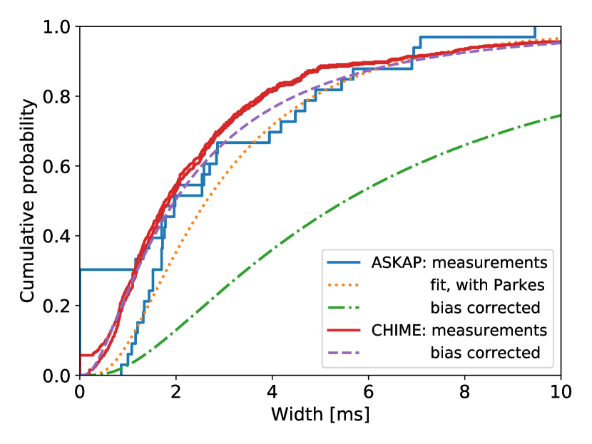
Figure 1: FRB width cumulative distributions. Shown are measurements from ASKAP (Qiu et al., 2020) and CHIME (CHIME/FRB Collaboration et al., 2021), with upper and lower lines calculated by assuming FRBs with upper limits have widths equal to zero and the limit value respectively. Also shown is a fit to data from ASKAP and Parkes (Arcus et al., 2021), and estimates of the bias-corrected (intrinsic) width distributions (J22a). The ASKAP and Parkes data have not had the effects of scattering removed. Note that we use the total FRB widths, which are twice the reported Gaussian standard deviations.

From Figure 1, the measured and bias-corrected width distributions found by CHIME (CHIME/FRB Collaboration et al., 2021) are broadly consistent with the measurements of ASKAP and Parkes (Qiu et al., 2020; Arcus et al., 2021, J22a), but narrower than the bias-corrected values (James et al., 2022a). This is an interesting result in-and-of itself, and assuming it is not due to some difference in the fitting methods, it may imply some frequency-dependent aspect of the FRB emission mechanism, or an unknown selection effect. It is also in contrast to the results of Gajjar et al. (2018), who find that the intrinsic width of bursts from FRB 20211102 decreases with increasing frequency. For our purposes however, we simply retain the previous bias-corrected width distribution from J22a, and add the contribution from scattering according to (15) and the parameters found by CHIME/FRB Collaboration et al. (2021).

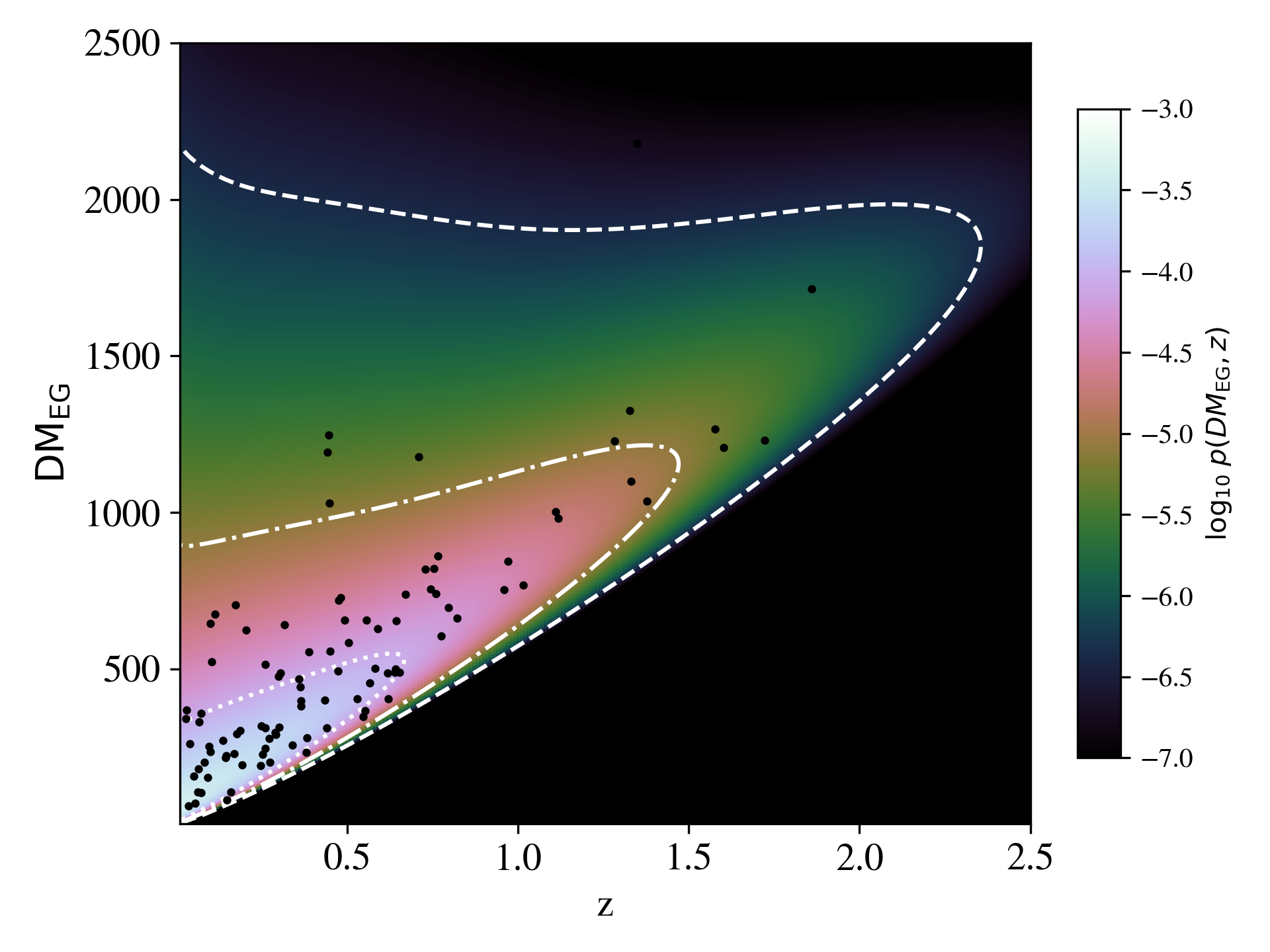
Figure 2: The color image describes $P(z,{\rm DM})$ for the forthcoming CRACO survey on the ASKAP telescope for a fiducial set of model parameters (Table 1). Overplotted are white contours enclosing 50% (dotted), 90% (dash-dot) and 99% (dashed) of the probability. The black dots are a Monte Carlo realization of the PDF for a random draw of 100 FRBs (Table 6).

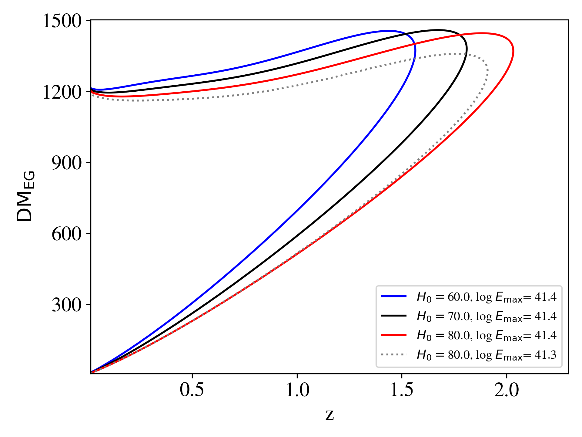
Figure 3: The colored curves are the 95% contours in the $P(z,{\rm DM})$ space for the fiducial CRACO model (Table 1) but with ${H_{0}}$ varying from 60 $\rm km\,s^{-1}\,Mpc^{-1}$ (blue) to 80 $\rm km\,s^{-1}\,Mpc^{-1}$(red). As ${H_{0}}$ increases, the contours tilt towards lower ${\rm DM}_{\rm EG}$ values due to the ${H_{0}}$^-1 dependence of $\langle{\rm DM}_{\rm cosmic}\rangle$ (Equation 9). They also extend to higher $z$ because higher ${H_{0}}$ implies a physically smaller universe, i.e. one can observe an FRB with given energy to higher $z$. This effect, however, is partially degenerate with the energetics of the FRB population as described by the dotted line (a model with lower $E_{\rm max}$).

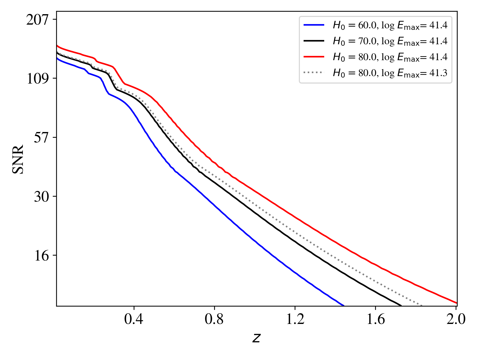
Figure 4: Similar to Figure 3 except the curves are contours in the $P(z,\rm SNR)$ space (95% of the events are expected to occur below the lines). While the models indicate significant ${H_{0}}$ dependence, these are more nearly degenerate with $E_{\rm max}$ than the results in the $P(z,{\rm DM})$ space, e.g, compare the solid, black curve with the dotted curve which have significantly differing ${H_{0}}$ and $E_{\rm max}$.

Table 1: Fiducial Set of Model Parameters. Parameters labelled with a * are re-fit as part of this work.

Parameter	Fiducial Value	Unit	Description
$\log_{10}\mu_{s}$	0.7	ms	Mean of log10-scattering distribution at 600 MHz
$\log_{10}\sigma_{s}$	1.9	ms	Standard deviation of log10-scattering distribution at 600 MHz
$\mu_{w}$	1.70267	ms	$\log_{10}$ mean of intrinsic width distribution in ms
$\sigma_{w}$	0.899148	ms	$\log_{10}$ sigma of intrinsic width distribution in ms
DMISM	NE2001	${\rm pc\,cm^{-3}}$	DM for the Milky Way Interstellar Medium
${\rm DM}_{\rm halo}$	50	pc cm-3	DM for the Galactic halo
$n_{\rm sfr}^{*}$	0.73		Scaling of FRB rate density with star-formation rate
$H_{0}^{*}$	67.66	km s-1 Mpc-1	Hubble’s constant
$\Omega_{\Lambda}$	0.68885		Dark energy / cosmological constant (in current epoch)
$\Omega_{m}$	0.30966		Matter density in current epoch
$\Omega_{b}$	0.04897		Baryon density in current epoch
$\Omega_{b}h^{2}$	0.02242		Baryon density weighted by $h_{100}^{2}$
$\mu_{\rm host}^{*}$	2.18		$\log_{10}$ mean of DM host contribution in pc cm-3
$\sigma_{\rm host}^{*}$	0.48		$\log_{10}$ sigma of DM host contribution in pc cm-3
$f_{d}(z=0)$	0.844		Fraction of baryons that are diffuse and ionized at $z=0$
$F$	0.32		F parameter in DMcosmic PDF for the Cosmic web
$\log_{10}E_{\rm min}$	30	erg	$\log_{10}$ of minimum FRB energy
$\log_{10}E_{\rm max}^{*}$	41.4	erg	$\log_{10}$ of maximum FRB energy
$\alpha^{*}$	0.65		Power-law index of frequency dependent FRB rate, $R\sim\nu^{\alpha}$
$\gamma^{*}$	-1.01		Slope of luminosity distribution function

3 Exploring the Model Dependencies on ${H_{0}}$

In this section, we consider examples of the forward model to gain intuition on the constraints for ${H_{0}}$ imposed by the observations as well as key model degeneracies. In the following, we assume properties for future FRB surveys on the ASKAP telescope using the CRAFT COherent upgrade (CRACO) system. Its characteristics follow the ICS (mid) survey performed on ASKAP by the CRAFT project but with approximately 4.4 times greater sensitivity due to the anticipated coherent addition of 24 antennas (as opposed to the incoherent addition of typically 25), and a slightly reduced bandwidth (from 336 MHz to 288 MHz).

Figure 2 shows the $P(z,{\rm DM})$ probability distribution function (PDF) for this CRACO survey and a fiducial set of model parameters (Table 1) informed by J22a. Overplotted is a Monte Carlo realization of 100 random FRBs drawn from the 2D PDF. These are, as expected, located primarily within the 90% contour in PDF. This Monte Carlo sample is analyzed in $\S$ 6 to perform a forecast on the future sensitivity of FRB surveys to ${H_{0}}$.

The $P(z,{\rm DM})$ PDF is highly asymmetric with a long tail to large ${\rm DM}_{\rm EG}$ values. This asymmetry is driven by the predicted tails in ${\rm DM}_{\rm cosmic}$ due to the Poisson nature of cosmic structure (e.g. large ${\rm DM}_{\rm cosmic}$ values from galaxy clusters) and the adopted log-normal PDF for ${\rm DM}_{\rm host}$. At the highest ${\rm DM}_{\rm EG}$ values ($>1500\,{\rm pc\,cm^{-3}}$), $P(z,{\rm DM})$ tends towards lower redshift. This counter-intuitive effect is due to the reduction in ${\rm SNR}$ by DM-smearing of the signal combined with simple cosmological dimming (Connor, 2019, J22a).

Now we consider differences in $P(z,{\rm DM})$ due to variations in ${H_{0}}$. Figure 3 shows the 95% contours in the $P(z,{\rm DM})$ plane for a range of ${H_{0}}$ values and two choices of $E_{\rm max}$. The results may at first seem counter-intuitive. In particular, the models with higher ${H_{0}}$ lean toward lower ${\rm DM}_{\rm EG}$ values in the $P(z,{\rm DM})$ plane even though ${\rm DM}_{\rm cosmic}\propto\Omega_{b}h$. This occurs because we have held $\Omega_{b}h^{2}$ fixed (see $\S$ 2.1) such that increasing ${H_{0}}$ decreases $\Omega_{b}h$ proportionally and therefore ${\rm DM}_{\rm cosmic}$ (Equation 9) and therefore ${\rm DM}_{\rm EG}$. Because the tail to high ${\rm DM}_{\rm EG}$ includes attributes of the host (${\rm DM}_{\rm host}$) and the distribution of baryons with the Universe’s cosmic web (parameterized by $F$ Macquart et al., 2020), the greatest constraining power on ${H_{0}}$ is from the lower boundary of the contours. This is evident in Figure 2 where one notes the sharpness of $P(z,{\rm DM})$ along the lower edge of the PDF contours.

Another important behaviour seen in Figure 3 is that the contours ‘rotate’ within the plane as ${H_{0}}$ varies. All of the other model parameters that significantly affect ${\rm DM}_{\rm EG}$ (e.g. those influencing ${\rm DM}_{\rm host}$) tend to rigidly shift and/or widen the contours parallel to ${\rm DM}_{\rm EG}$. Therefore, there is significant constraining power in the data for ${H_{0}}$ without high degeneracy.

The other notable effect of increasing ${H_{0}}$ is that the contours extend to higher redshift. With all other cosmological parameters fixed (except $\Omega_{b}$), a universe with higher ${H_{0}}$ is ‘smaller’. Surveys with a given flux sensitivity can therefore observe FRBs to higher redshift. This secondary effect, however, is partially degenerate with the FRB luminosity function and especially $E_{\rm max}$. Figure 3 shows an additional contour with ${H_{0}}=80\,\rm km\,s^{-1}\,Mpc^{-1}$ and an $E_{\rm max}$ value 20% lower than the fiducial value. Lowering $E_{\rm max}$ reduces the redshift extent of the ${H_{0}}=80\,\rm km\,s^{-1}\,Mpc^{-1}$ to be similar to that with a higher $E_{\rm max}$ and ${H_{0}}=70\,\rm km\,s^{-1}\,Mpc^{-1}$, although the contours remain offset. This also suggests some sensitivity to the functional form of the luminosity function of (14). We further investigate correlations between ${H_{0}}$ and $E_{\rm max}$ when fitting to data in §5.3.

This coupling of ${H_{0}}$ and $E_{\rm max}$ manifests in the other primary FRB observable: $s$. Put another way, to the extent that energetics of the FRB phenomenon are invariant with redshift the analysis is effectively a standard candle. We illustrate the model dependence in Figure 4 which shows the PDF of $P(z,\rm SNR)$ for several choices of ${H_{0}}$ and $E_{\rm max}$. There is a strong ${H_{0}}$ dependence on the predicted distribution for $s$ as a function of redshift, but the variance is nearly degenerate with $E_{\rm max}$, e.g. decreasing ${H_{0}}$ by 10 $\rm km\,s^{-1}\,Mpc^{-1}$ is nearly equivalent to lowering $E_{\rm max}$ by 0.1 dex (compare the black solid and dotted curves in Figure 4).

Table 2: ASKAP incoherent sum FRBs used in this analysis. Given is the FRB name, SNR-maximising DM, ${\rm DM}_{\rm ISM}$ estimated using the NE2001 model of Cordes & Lazio (2002), central frequency of observation $\nu$, measured signal-to-noise ratio SNR, redshift $z$, posterior probability of host associations $P(O|x)$, and original reference. Where redshifts are not given, this is because (a): no voltage data were dumped, preventing radio localization; (b) optical follow-up observations are not yet complete; (c) Substantial Galactic extinction has challenged follow-up optical observations; (d) the host galaxy appears too distant to accurately measure a redshift.

Name	DM	${\rm DM}_{\rm ISM}$	$\nu$	SNR	$z$	$P(O|x)$	Ref.
	(${\rm pc\,cm^{-3}}$)	(${\rm pc\,cm^{-3}}$)	(MHz)
CRAFT/ICS $900\,{\rm MHz}$
20191001	506.92	44.2	919.5	62.0	0.23	0.973	Bhandari et al. (2020)
20200430	380.1	27.0	864.5	16.0	0.161	1.000	Heintz et al. (2020)
20200906	577.8	35.9	864.5	19.2	0.36879	1.000	Bhandari et al. (2022)
20210807	251.9	121.2	920.5	47.1	0.12927	0.957	Deller et al. (in prep.)
20200627	294.0	40.0	920.5	11.0	(a)	n/a	Shannon et al. (in prep.)
20210320	384.8	42.2	864.5	15.3	0.2797	0.999
20210809	651.5	190.1	920.5	16.8	(a)	n/a
20211203	636.2	63.4	920.5	14.2	(b)	n/a
CRAFT/ICS $1.3\,{\rm GHz}$
20180924	362.4	40.5	1297.5	21.1	0.3214	0.999	Bannister et al. (2019)
20181112	589.0	40.2	1297.5	19.3	0.4755	0.927	Prochaska et al. (2019b)
20190102	364.5	57.3	1271.5	14	0.291	1.000	Macquart et al. (2020)
20190608	339.5	37.2	1271.5	16.1	0.1178	1.000
20190611.2	322.2	57.6	1271.5	9.3	0.378	0.980
20190711	594.6	56.6	1271.5	23.8	0.522	0.999
20190714	504.7	38.5	1271.5	10.7	0.209	1.000	Heintz et al. (2020)
20191228	297.5	32.9	1271.5	22.9	0.243	1.000	Bhandari et al. (2022)
20210117	730	34.4	1271.5	27.1	0.2145	0.999	Bhandari et al. (in prep.)
20210214	398.3	31.9	1271.5	11.6	(a)	n/a	Shannon et al. (in prep.)
20210407	1785.3	154	1271.5	19.1	(c)	n/a
20210912	1234.5	30.9	1271.5	31.7	(d)	n/a
20211127	234.83	42.5	1271.5	37.9	0.0469	0.998	Deller et al. (in prep.)
CRAFT/ICS $1.6\,{\rm GHz}$
20211212	206	27.1	1632.5	12.8	0.0715	0.998	Deller et al. (in prep.)

4 Observational Sample

The FRBs analyzed here mainly draw from the same samples of J22a and we refer the reader to that manuscript for full details. Briefly, the three samples used are FRBs detected by the Murriyang (Parkes) Multibeam system (Parkes/Mb; e.g. Staveley-Smith et al., 1996; Keane et al., 2018), ASKAP when observing in Fly’s Eye mode (CRAFT/FE; Bannister et al., 2017), and ASKAP when observing in incoherent sum mode (CRAFT/ICS; Bannister et al., 2019, Shannon et al. (in prep.)). Here we describe updates to this data set, and the methods used to address bias in the data.

Our criteria aim to be inclusive in our data selection, in order to overcome the limitations from the small number of localized FRBs. The studies presented in Appendix A suggest that any systematic effects of doing so will be small compared to the statistical error due to small sample size. We expect to revise these criteria when more data become available. See J22a for a discussion of observational biases against high-DM FRBs.

4.1 New localized FRBs

Since the publication of J22a, the CRAFT survey has continued to observe commensally in incoherent sum mode. While observations are still ongoing, we include all FRBs detected up to Dec 31^st 2021. This adds 14 new FRBs to our sample. Their relevant properties are listed in Table 2, while their detailed properties will be given in several works currently in preparation (Deller et al. (in prep.); Shannon et al. (in prep.), Gordon et al., in prep.).

4.2 Addition of FRBs with higher ${\rm DM}_{\rm ISM}$

Table 3: Properties of CRAFT/FE and Parkes/Mb FRBs previously excluded due to their relatively high ${\rm DM}_{\rm ISM}$, which are now included in this analysis. Given is the original FRB designation; measured total DM and DM_ISM estimated by the NE2001 model (Cordes & Lazio, 2002) in pc cm^-3, and ratio of measured to threshold SNR.

FRB	DM	DMISM	SNR	Ref.
Parkes/Mb
20150610	1593.9	104	18	Bhandari et al. (2018)
20151206	1909.8	239	10
20171209	1457.4	329	40	Osłowski et al. (2019)
20180714	1467.92	254	22
20150418	776.2	164	39	Keane et al. (2016)
20010125	790	105	17	Burke-Spolaor & Bannister (2014)
20010621	745	502	16.3	Keane et al. (2011)
20150215	1105.6	405	19	Petroff et al. (2017)
CRAFT/FE
20180315	479.0	100.8	10.5	Macquart et al. (2019)
20180430	264.1	169	28.2	Qiu et al. (2019)

In J22a, only FRBs with ${\rm DM}_{\rm ISM}<100$ ${\rm pc\,cm^{-3}}$ were included in the analysis. This is because higher values of ${\rm DM}_{\rm ISM}$ degrade sensitivity to FRBs, and it is too computationally expensive to calculate sensitivity for each individual FRB. Rather, the simulation uses the mean value of ${\rm DM}_{\rm ISM}$ for the sample to calculate this observation bias, while using individual values of ${\rm DM}_{\rm ISM}$ to calculate ${\rm DM}_{\rm EG}$ for the purposes of likelihood evaluation. This criterion previously rejected eight FRBs from Parkes/Mb, and two FRBs from CRAFT/FE. We show in Appendix A.2 that this criterion can be relaxed somewhat, and we now include all previously excluded FRBs. This includes FRB 20010621, which we consider has sufficient excess DM beyond the estimated ${\rm DM}_{\rm ISM}$ to be classified as an (extragalactic) FRB. These are listed in Table 3. In the future, when larger numbers of localised FRBs reduce statistical errors, the very small bias due to this approximation could become relevant, and this criterion may have to be revisited.

4.3 Extension to other frequency ranges

ASKAP/CRAFT observations in ICS mode are predominantly fully commensal. This means that FRBs may be detected in any of the four ASKAP observing bands, covering 600-1800 MHz (Hotan et al., 2021). Within each band, the precise choice of which 336 1 MHz frequency channels are available to the CRAFT system also varies on a per-observation basis. Typically however, observations have clustered around two main frequency ranges near $900$ MHz and $1.3$ GHz, with a few further observations near 1.6 GHz. We label these ranges CRAFT/ICS $900\,{\rm MHz}$, CRAFT/ICS $1.3\,{\rm GHz}$, and CRAFT/ICS $1.6\,{\rm GHz}$ respectively. We therefore calculate $P(N_{\rm FRB})$, the probability of detecting a total of $N_{\rm FRB}$ FRBs, and $P(z,{\rm DM},\rm SNR)$ separately for each of these three frequency ranges, and treat these as independent surveys, with $N_{\rm FRB}$ equal to 8 FRBs, 13 FRBs, and 1 FRB respectively. For computational simplicity, as per J22a, within each survey we average the sensitivity over several observation-to-observation differences, such as the number of summed antennas (typically 25), observation frequency, beam configuration, system temperature, and time resolution, as well as ${\rm DM}_{\rm ISM}$ as discussed above (however, ${\rm DM}_{\rm EG}$ is calculated individually for each FRB).

The extension to frequencies beyond the nominal 1.3 GHz addressed by J22a also requires considering the effects of scattering separately from the intrinsic FRB width, as discussed in §2.2.3. It does however allow the inclusion of FRB 20191001, which was excluded from J22a as being the only FRB at the time of analysis to be discovered in CRAFT/ICS observations outside the 1.3 GHz band.

4.4 Consideration of host galaxy probability

The redshifts associated with each localised FRB are derived from observations of the host galaxy — which necessarily requires a firm association of the FRB with that galaxy. The Probabilistic Association of Transients to their Hosts (PATH; Aggarwal et al., 2021) gives a method to calculate posterior probabilities $P(O|x)$ of any given host galaxy association, while accounting for FRB localisation uncertainties. In the original analysis, seven of nine CRAFT/ICS FRB host galaxies associations were found with $P(O|x)\ >95$%.

Bhandari et al. (2022) has performed an updated PATH analysis of three localized CRAFT FRBs, and reported a posterior probability $P(O|x)$ for the host association exceeding 90% in each case. In Shannon et al. (in prep.) we argue that one should modify the standard PATH priors introduced by Aggarwal et al. (2021) which increases the $P(O|x)$ values for these and all previous FRBs from CRAFT/ICS. Thus all localised FRBs in our sample have posterior values of $P(O|x)$ of 90% or greater, as listed in Table 2.

4.5 CRAFT/ICS FRBs with no hosts

The results and forecasts presented thus far have implicitly assumed that we have observed a complete and unbiased sample from the FRB surveys. We recognize, however, that there is no perfect FRB survey nor related follow-up efforts (e.g. to obtain the FRB redshift). Of the FRBs included in Table 2, six have no identified host. There are many potential reasons for this (numbers are for the current sample in Table 2):

1. the buffered data necessary for localisation was not available for technical reasons (3 FRBs);

2. the FRB host is obscured either by proximity to bright stars, or by high levels of dust extinction in the Milky Way (1 FRB);

3. the FRB host has not been observed yet, due to being too close to the Sun, or simply because the FRB is so recent that observations have not yet been completed (1 FRB);

4. the FRB host cannot be identified amongst several candidate galaxies (no FRBs yet);

5. the FRB host is too distant or faint to be detected with ground-based follow-up observations (1 FRB).

It is critical therefore that these effects do not introduce biases into our analysis.

Of the above, reasons 1, 2 and 3 are clearly uncorrelated with the properties of the FRBs themselves, so that while missing these FRBs reduces our statistical power, using $P({\rm DM})$ rather than $P(z,{\rm DM})$ introduces no bias. Reason 4 is a function of both the radio localization accuracy, and the number and properties of galaxies in the FRB field. While more distant FRBs are on-average dimmer (Shannon et al., 2018), and thus will have a greater statistical error on their localization, the correlation between SNR and $z$ is relatively weak; furthermore, the localization accuracy of CRAFT/ICS FRBs is typically dominated by systematics in FRB image alignment (Day et al., 2021), which are uncorrelated with FRB properties. However, since angular diameter distance is increasing over the redshift range of observed CRAFT/ICS FRBs, a constant angular resolution will result in a more-difficult host galaxy identification with increasing $z$, making it more likely to preferentially reject FRBs from high redshifts. Furthermore, one may not be able to obtain a sufficiently high-quality spectrum of the galaxy to confidently measure its redshift. Reason 5 is clearly correlated with redshift: an FRB follow-up observation probing to a limiting r-band magnitude of 22 might be insufficient to detect a 0.1 $L^{*}$ galaxy beyond $z=1$ or a 0.01 $L^{*}$ galaxy beyond a redshift of 0.1 (Eftekhari & Berger, 2017).

We deal with these biases here by choosing a maximum extragalactic dispersion measure, DM${}_{\rm EG}^{\rm max}=1000$ ${\rm pc}\,{\rm cm}^{-3}$, beyond which detected FRBs are classified as unlocalised regardless of whether or not their host has been identified. To avoid bias in redshift, it is critical that this criterion is independent of $z$; however, these FRBs must be included in the calculation of $P({\rm DM})$ to avoid bias in that parameter. Our localizations are sufficiently certain that we are not currently affected by reason 4. FRBs which are unlocalized for any other reason are also included in the calculation of $P({\rm DM})$ — rejecting these would not introduce a bias, but would reduce the statistical power of the sample. We show in Appendix A.3 how this procedure allows an unbiased measure of ${H_{0}}$. In total, six CRAFT/ICS FRBs are treated this way — see Table 2.

4.6 Observation time, and low SNR bias

The question of observational bias against low-SNR FRBs has a long history (Macquart & Ekers, 2018a; James et al., 2019c). An analysis of the measured SNR of CRAFT/ICS FRBs however reveals that the majority of FRBs with SNR$\lesssim 15$ have been undetected, resulting in a total FRB rate which is approximately half that expected (Shannon et al., in prep.). Under the simplifying assumption of a Euclidean slope of $(N_{\rm FRB}>{\rm SNR})\propto{\rm SNR}^{-1.5}$, we expect that for every FRB detected with ${\rm SNR}\geq 15$, 1.15 are detected in the range $9\leq{\rm SNR}\leq 15$, where ${\rm SNR}_{\rm th}=9$ is the nominal CRAFT/ICS detection threshold. However, CRAFT/ICS have detected 16 FRBs with ${\rm SNR}\geq 15$, and only 6 with ${\rm SNR}\leq 15$, when 18.4 might be expected. Some of the missing low-SNR FRBs can be attributed to periods of high RFI ($\lesssim 10\%$ of the searches) where the detection threshold had to be raised as high as ${\rm SNR}_{\rm th}=14$; however, in most cases this loss remains unexplained. We note that there is no evidence for such a bias in CRAFT/FE data; nor does there appear to be a correlation between missing FRBs and properties such as DM or frequency, although our ability to probe this is affected by low sample numbers.

The assumption of a 50% loss of FRBs due to a bias against low-SNR events is also backed up by calculations of the absolute CRAFT/ICS $1.3\,{\rm GHz}$ FRB rate (Shannon et al., in prep), which was not available in time for use in J22a. The expected rate of CRAFT/ICS $1.3\,{\rm GHz}$ FRBs is relatively model-independent, since the frequency range is almost identical to — and the sensitivity lies between — CRAFT/FE and Parkes/Mb observations. This reveals a detection rate which is approximately half that expected, which is consistent with the low-SNR bias described above.

We account for this issue therefore by taking the absolute observation time of CRAFT/ICS observations measured by Shannon et al. (in prep), and divide by half, to represent the 50% loss of detection efficiency. Importantly, the measured FRB rate of CRAFT/ICS $900\,{\rm MHz}$ and CRAFT/ICS $1.6\,{\rm GHz}$ observations allows us to have better statistical inference on the frequency-dependent rate parameter $\alpha$, which aside from a prior based on the results of Macquart et al. (2019), was largely unconstrained in J22a. In Appendix A.1, we demonstrate that missing FRBs in this small SNR range does not cause any significant bias in the determination of ${H_{0}}$, so we retain the threshold of ${\rm SNR}_{\rm th}=9.0$.

5 Results

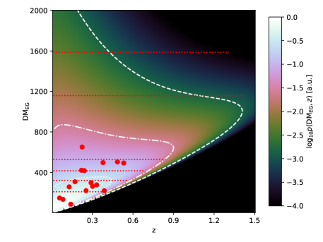
Figure 5: The z–DM distribution of FRBs (shading) using best-fitting model parameters, summed over the CRAFT/ICS $900\,{\rm MHz}$, CRAFT/ICS $1.3\,{\rm GHz}$, and CRAFT/ICS $1.6\,{\rm GHz}$ samples. Also shown are FRBs with (red solid circles) and without (red dashed lines) host galaxy redshifts. The latter are drawn at their estimated values of ${\rm DM}_{\rm EG}$ out to $z_{99}$, i.e. encompassing 99% of their likelihood in $P(z|{\rm DM})$ for their ${\rm DM}_{\rm EG}$ values. White contours of dotted, dash-dot, and dashed lines encompass 50%, 90%, and 99% of the probability density of $P(z,{\rm DM})$ respectively.

Parameter	Min	Max	Increment
${H_{0}}$	55	101	2
$\log_{10}E_{\rm max}$	40.5	42.5	0.1
$\alpha$	0	2	0.5
$\gamma$	-1.5	-0.5	0.1
$n$	0	3	0.25
$\mu_{\rm host}$	1.5	2.6	0.1
$\sigma_{\rm host}$	0.3	1.1	0.1

Table 4: Parameters and their values (in linear increments from min to max values) at which the joint likelihood $P(z,{\rm DM},\rm SNR)$ was evaluated. $\log_{10}E_{\rm min}$ was fixed at $10^{30}$ erg.

We evaluate $P(N_{\rm FRB})$ for each survey, and $P(z,{\rm DM},\rm SNR)$ for each FRB in that survey, over a seven-dimensional cube of parameters, with values given in Table 4. Posterior probabilities are calculated from the resulting product over all FRBs and surveys using uniform priors over the simulated parameter ranges, while confidence intervals on those parameters are constructed using the prescription of Feldman & Cousins (1998). Our results are given below. The best-fitting z–DM distribution for ASKAP FRBs is shown in Figure 5.

5.1 ${H_{0}}$

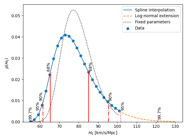
Figure 6: Posterior probability on ${H_{0}}$, using cubic splines (blue solid curve) fitted to data points (circles), using uniform priors over the simulated range, and extrapolated to higher values of ${H_{0}}$ using a log-normal fit (orange dashed curve). Confidence intervals are also shown (vertical red lines). The posterior probability when fixing all other parameters to their best-fit values is also shown (grey dotted curve).

Our posterior probability distribution for ${H_{0}}$ is given in Figure 6. We simulate only up to ${H_{0}}$=103 $\rm km\,s^{-1}\,Mpc^{-1}$: in the range above 80 $\rm km\,s^{-1}\,Mpc^{-1}$, we find the probability to be decreasing as a log-normal to better than 1% relative accuracy, so we save significant compute time and extrapolate results to ${H_{0}}$=130 $\rm km\,s^{-1}\,Mpc^{-1}$. Our best-fit value is ${H_{0}}$=$73_{-8}^{+12}$ $\rm km\,s^{-1}\,Mpc^{-1}$. While this agrees with values of ${H_{0}}$ derived from near-Universe measures, it is also consistent within $1\,\sigma$ of indirect values derived from e.g. the CMB (Abdalla et al., 2022).

Our constraint on ${H_{0}}$ is not symmetric — we derive a relatively sharp lower boundary, with looser constraints on large values of ${H_{0}}$. This is the result of what we term ‘the cliff effect’, whereby large excess DMs above the mean can be induced by intersection with galaxy halos or host galaxy contributions, but even voids contribute a minimum ${\rm DM}_{\rm cosmic}$. Thus, probability distribution $P(z|{\rm DM})$ has a sharp lower cutoff, or ‘cliff’. Low values of ${H_{0}}$ thus imply a higher minimum DM as a function of $z$, and when this minimum is contradicted by even a single measured FRB, those values of ${H_{0}}$ can be excluded. Higher values of ${H_{0}}$ however do not suffer such a large penalty due to the long tail of the $P({\rm DM}|z)$ distribution.

Figure 6 also shows the constraint on ${H_{0}}$ we would derive if all other FRB parameters are fixed to their best-fit values. This demonstrates the importance of performing a multi-parameter fit and marginalising over nuisance parameters. Even in the case that the fixed values of FRB parameters are well-guessed (i.e. at the best-fitting values used here), ignoring the confounding effects of uncertainties in these parameters nonetheless leads to a biased and artificially too-precise estimate of ${H_{0}}$.

Figure 7: Posterior probability on ${H_{0}}$, using cubic splines (solid curves) fitted to data points (squares), using uniform priors over the simulated range, for each of the five FRB surveys used in this work.

It is also interesting to examine the constraints on ${H_{0}}$ from each FRB survey individually. This is shown in Figure 7. The two surveys with large numbers of localised FRBs — CRAFT/ICS $900\,{\rm MHz}$ and CRAFT/ICS $1.3\,{\rm GHz}$ — provide the dominant constraints, as expected. That CRAFT/ICS $1.3\,{\rm GHz}$ is better fit by a higher value of ${H_{0}}$ is due to the cliff effect and FRB 20190102, which has a very low DM of 322.2 ${\rm pc\,cm^{-3}}$ for its redshift of 0.378. That the single localised FRB of CRAFT/ICS $1.6\,{\rm GHz}$ provides a comparable amount of information to CRAFT/FE and Parkes/Mb, with 26 and 28 FRBs each, illustrates the importance of localised FRB samples when constraining ${H_{0}}$.

5.2 Constraints on other parameters

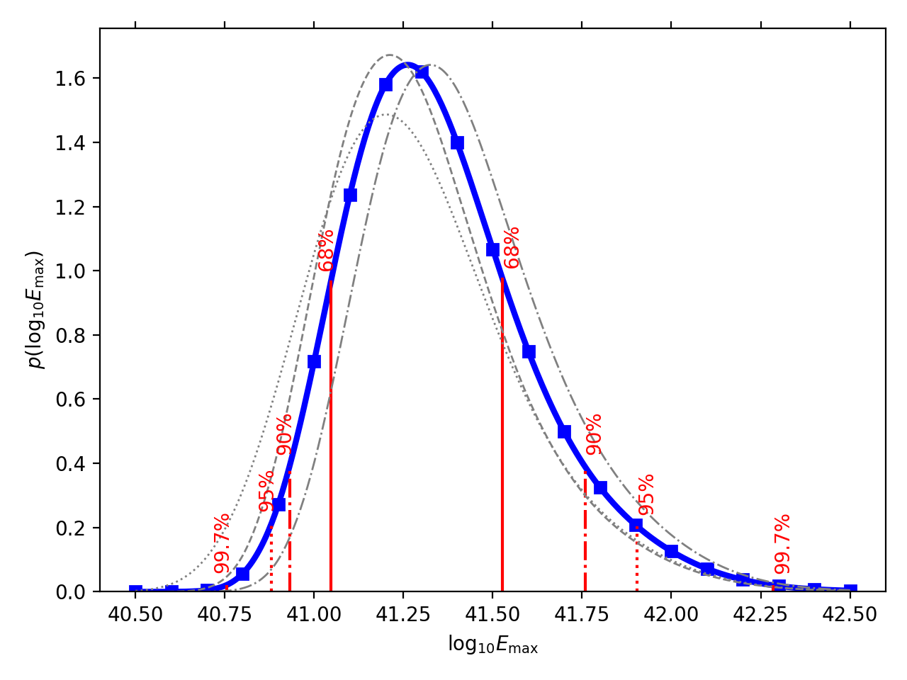
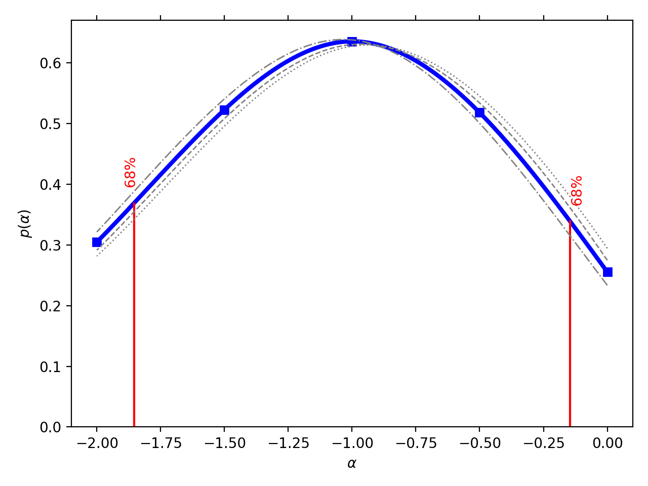
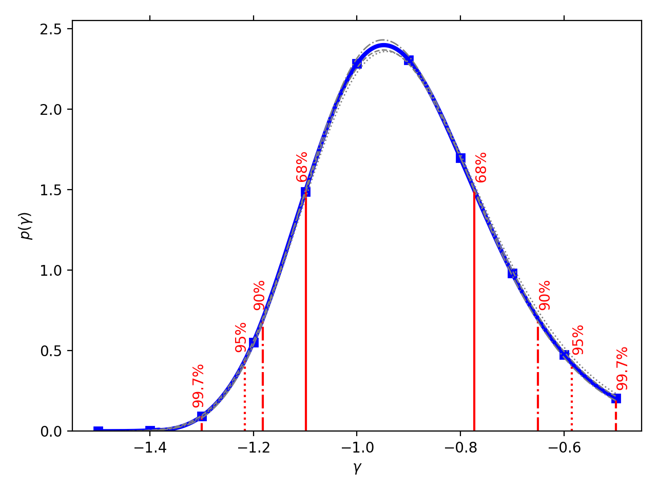
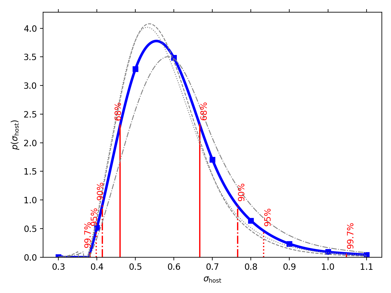
Figure 8: Posterior probabilities on the six other estimated parameters, using a prior for ${H_{0}}$ based on CMB and SN1a results (blue curves; see text). Also shown are posterior probabilities with no prior on ${H_{0}}$ (grey dotted curves) and with ${H_{0}}$ fixed to 67 $\rm km\,s^{-1}\,Mpc^{-1}$(grey dashed curves) and 73 $\rm km\,s^{-1}\,Mpc^{-1}$(grey dash-dot curves).

Table 5: Best-fitting parameter values and associated confidence intervals for each fitted parameter. For parameters other than ${H_{0}}$, limits are given for different priors on ${H_{0}}$: the ‘standard’ prior, covering both early- and local-Universe measurements of ${H_{0}}$ (see text); fixing ${H_{0}}$ to 67.4 $\rm km\,s^{-1}\,Mpc^{-1}$ and 73.04 $\rm km\,s^{-1}\,Mpc^{-1}$; and a flat prior between 55 and 101 $\rm km\,s^{-1}\,Mpc^{-1}$. For $\alpha$, only approximate 68 per cent errors are given (see text).

			68 per	90 per	95 per	99.7 per
Parameter	Prior	Best Fit	cent	cent	cent	cent
$H_{0}$	N/A	73.0	${}_{-8}^{+12}$	${}_{-12}^{+22}$	${}_{-13}^{+29}$	${}_{-17}^{+48}$
$\log_{10}E_{\rm max}$	Std	$41.26$	${}_{-0.22}^{+0.27}$	${}_{-0.33}^{+0.50}$	${}_{-0.38}^{+0.64}$	${}_{-0.51}^{+1.02}$
	Flat	$41.20$	${}_{-0.25}^{+0.29}$	${}_{-0.39}^{+0.52}$	${}_{-0.45}^{+0.67}$	${}_{-0.61}^{+1.06}$
	73.04	$41.21$	${}_{-0.21}^{+0.26}$	${}_{-0.32}^{+0.49}$	${}_{-0.37}^{+0.63}$	${}_{-0.49}^{+1.03}$
	67.4	$41.33$	${}_{-0.22}^{+0.27}$	${}_{-0.33}^{+0.50}$	${}_{-0.38}^{+0.63}$	${}_{-0.50}^{+0.99}$
$\alpha$	Std	$-0.99$	${}_{-1.01}^{+0.99}$	N/A
	Flat	$-0.92$	${}_{-1.08}^{+0.92}$	N/A
	73.04	$-0.95$	${}_{-1.05}^{+0.95}$	N/A
	67.4	$-1.03$	${}_{-0.97}^{+1.03}$	N/A
$\gamma$	Std	$-0.95$	${}_{-0.15}^{+0.18}$	${}_{-0.23}^{+0.30}$	${}_{-0.27}^{+0.36}$	${}_{-0.36}^{+0.45}$
	Flat	$-0.94$	${}_{-0.15}^{+0.18}$	${}_{-0.24}^{+0.30}$	${}_{-0.27}^{+0.37}$	${}_{-0.36}^{+0.44}$
	73.04	$-0.95$	${}_{-0.15}^{+0.18}$	${}_{-0.23}^{+0.30}$	${}_{-0.27}^{+0.37}$	${}_{-0.36}^{+0.45}$
	67.4	$-0.95$	${}_{-0.15}^{+0.17}$	${}_{-0.23}^{+0.29}$	${}_{-0.27}^{+0.36}$	${}_{-0.35}^{+0.45}$
$n_{\rm sfr}$	Std	$1.13$	${}_{-0.41}^{+0.49}$	${}_{-0.65}^{+0.77}$	${}_{-0.77}^{+0.90}$	${}_{-1.09}^{+1.19}$
	Flat	$1.08$	${}_{-0.41}^{+0.50}$	${}_{-0.64}^{+0.78}$	${}_{-0.76}^{+0.92}$	${}_{-1.05}^{+1.21}$
	73.04	$1.10$	${}_{-0.41}^{+0.50}$	${}_{-0.63}^{+0.78}$	${}_{-0.75}^{+0.92}$	${}_{-1.06}^{+1.21}$
	67.4	$1.15$	${}_{-0.41}^{+0.49}$	${}_{-0.66}^{+0.76}$	${}_{-0.79}^{+0.89}$	${}_{-1.11}^{+1.18}$
$\mu_{\rm host}$	Std	$2.27$	${}_{-0.13}^{+0.12}$	${}_{-0.23}^{+0.21}$	${}_{-0.28}^{+0.26}$	${}_{-0.47}^{+0.33}$
	Flat	$2.33$	${}_{-0.14}^{+0.13}$	${}_{-0.25}^{+0.21}$	${}_{-0.31}^{+0.25}$	${}_{-0.57}^{+0.27}$
	73.04	$2.30$	${}_{-0.12}^{+0.11}$	${}_{-0.20}^{+0.19}$	${}_{-0.25}^{+0.24}$	${}_{-0.40}^{+0.30}$
	67.4	$2.23$	${}_{-0.14}^{+0.13}$	${}_{-0.25}^{+0.22}$	${}_{-0.31}^{+0.28}$	${}_{-0.51}^{+0.37}$
$\sigma_{\rm host}$	Std	$0.55$	${}_{-0.09}^{+0.12}$	${}_{-0.13}^{+0.22}$	${}_{-0.16}^{+0.30}$	${}_{-0.21}^{+0.51}$
	Flat	$0.53$	${}_{-0.08}^{+0.11}$	${}_{-0.13}^{+0.22}$	${}_{-0.15}^{+0.29}$	${}_{-0.20}^{+0.52}$
	73.04	$0.54$	${}_{-0.08}^{+0.11}$	${}_{-0.13}^{+0.20}$	${}_{-0.15}^{+0.27}$	${}_{-0.20}^{+0.48}$
	67.4	$0.57$	${}_{-0.09}^{+0.13}$	${}_{-0.14}^{+0.25}$	${}_{-0.17}^{+0.33}$	${}_{-0.21}^{+0.51}$

Besides constraints on ${H_{0}}$, our addition of new localized FRBs yields greater statistical power to constrain the other fitted parameters — $\log_{10}E_{\rm max}$, $\alpha$, $\gamma$, $n_{\rm sfr}$, $\mu_{\rm host}$, and $\sigma_{\rm host}$ — while also accounting for the confounding effect of allowing ${H_{0}}$ to vary. However, since our constraint on ${H_{0}}$ using FRB data only is significantly less than that of other measurements, we apply a prior on ${H_{0}}$ which is flat between the best-fit CMB and SN1A values (67.4 and 73.04 $\rm km\,s^{-1}\,Mpc^{-1}$), and falls away as a Gaussian on the lower/upper regions with the respective uncertainties of those measurements (0.5 and 1.42 $\rm km\,s^{-1}\,Mpc^{-1}$).

Posterior probability distributions on these parameters are shown in Figure 8, while confidence limits on all parameters are reported in Table 5. For comparison, we also show results with no prior on ${H_{0}}$, which give worse constraints; and also results when assuming ${H_{0}}$ is fixed to either the value of 67.4 obtained by Planck Collaboration et al. (2020) or 73.04 from Riess et al. (2021), representing the improvement in accuracy should ${H_{0}}$ be known exactly.

We confirm the result of James et al. (2022b) that the FRB population exhibits cosmological source evolution consistent with the star-formation rate, excluding no source evolution ($n=0$) at $3\,\sigma$. This is in-line with the expectations from models predicting a close association between star-forming activity and FRB progenitors, in particular young magnetar models (e.g. Metzger et al., 2017), but does not exclude that a fraction of FRBs could arise from channels with a significant ($\sim$Gyr) characteristic delay from star formation, such as mergers. It does exclude that the majority of FRB progenitors have a cosmologically significant delay with respect to star formation. We observe that other results in the literature that analyse FRB population evolution (e.g. Cao et al., 2018; Locatelli et al., 2019; Arcus et al., 2021; Bhattacharyya et al., 2022) tend to assume a 1–1 z–DM (i.e. a purely linear) relationship, and/or fix values of other FRB population parameters, which are assumptions which we do not make.

We also find an increased value of $\mu_{\rm host}=2.27_{-0.13}^{+0.12}$, i.e. a median host DM of $186^{+59}_{-48}$ ${\rm pc\,cm^{-3}}$(the corresponding mean DM is 240 ${\rm pc\,cm^{-3}}$), which is significantly greater than the usually assumed value of 100 ${\rm pc\,cm^{-3}}$ found in the literature. This may not reflect entirely upon the actual FRB host galaxy: our fit to $\mu_{\rm host}$ will include any error in our assumed mean value of ${\rm DM}_{\rm halo}$=50${\rm pc\,cm^{-3}}$, and some component of $\sigma_{\rm host}$ will include scatter about that mean, and also errors in ${\rm DM}_{\rm ISM}$. However, since our used values of ${\rm DM}_{\rm halo}$=50${\rm pc\,cm^{-3}}$, and NE2001 for ${\rm DM}_{\rm ISM}$, are typical of the literature, it does suggest that the average work on FRBs is underestimating some combination of ${\rm DM}_{\rm host}$, ${\rm DM}_{\rm ISM}$, and/or ${\rm DM}_{\rm halo}$, and thus over-estimating ${\rm DM}_{\rm cosmic}$. Other results, such as the excess DM of $\sim 900$ ${\rm pc\,cm^{-3}}$ observed for FRB20190520B by Niu et al. (2022), and the suggestion of correlation between the locations of CHIME FRBs and large-scale structure at an excess DM of $\sim 400$ ${\rm pc\,cm^{-3}}$(Rafiei-Ravandi et al., 2021), support this conclusion.

The slope of the intrinsic luminosity function, $\gamma$, is found to be $-0.95^{+0.18}_{-0.15}$ — consistent with the observed high-energy slope of the luminosity functions of known repeating FRBs, e.g. $\gamma=-0.85\pm 0.3$ (Li et al., 2021), $-0.88>\gamma>-1.29$ (Jahns et al., 2022), and $\gamma=-1.04\pm 0.02$ (Hewitt et al., 2022) for FRB 20121102A. This is consistent with, though not sufficient proof of, apparently once-off FRBs being simply the high-energy tails of intrinsically repeating objects.

The posterior distribution of $\alpha$ drops only to approximately half its peak value over our simulated range ($-2\leq\alpha\leq 0$), suggesting an uncertainty of $\pm 0.85$. Thus we should consider that we have used a uniform top-hat prior on $\alpha$. Nonetheless, unlike J22a, we have significant discrimination power on $\alpha$. Our best-fit value of $\alpha=-1.0\pm 0.85$ is consistent with the result of Macquart et al. (2019), who find $\alpha=-1.5_{-0.3}^{+0.2}$ under the assumption that each FRB is characteristically broadband with a spectral slope, which (as argued in J22a) should be revised to $\alpha=-0.65^{+0.2}_{-0.3}$ under the ‘rate approximation’ used here. This disfavours the results of CHIME/FRB Collaboration et al. (2021) and Farah et al. (2019) — which do not include the effects of observational bias — that there is no increase of the FRB rate at decreasing frequency.

We conclude this section by noting that none of the above results are strongly dependent on our choice of prior on ${H_{0}}$ (none; based on existing literature; or fixed), with the greatest effect being on $E_{\rm max}$ and $\mu_{\rm host}$.

5.3 Correlations with other parameters

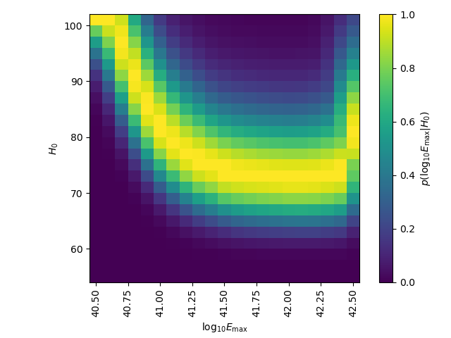
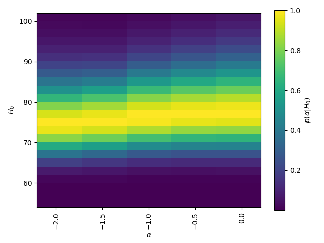
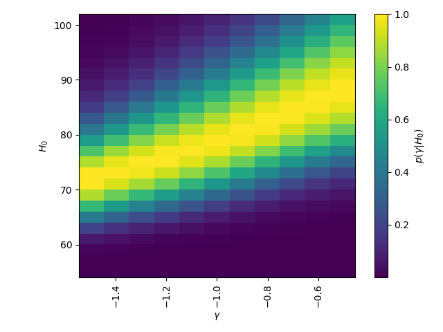
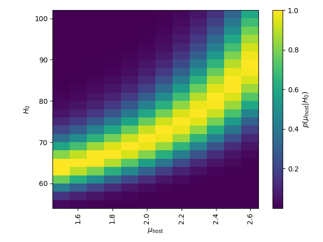
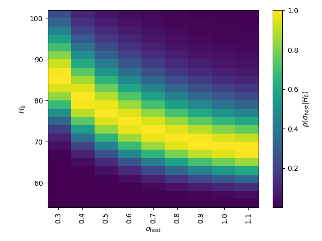
Figure 9: Conditional posterior probabilities on ${H_{0}}$ when allowing only single parameters to vary from their best-fit values. These plots describe degeneracies in the results between ${H_{0}}$ and the other model parameters.

We illustrate the correlations between parameters in Figure 9. We only show results for correlations between ${H_{0}}$ and other parameters, since J22a has already analysed other correlations. For each plot, we hold all other parameters constant at their best-fit values and plot the conditional probability $p(H_{0}|X)$ for each parameter $X$. From Figure 9, ${H_{0}}$ is correlated with all modelled parameters, emphasising the importance of jointly fitting them.

Some correlations are readily understood. As $\mu_{\rm host}$ increases, the implied ${\rm DM}_{\rm cosmic}$ decreases, favouring smaller distances being travelled by the FRB — and hence larger values of ${H_{0}}$. The strong negative correlation of ${H_{0}}$ with low values of $E_{\rm max}$ is because smaller values of $E_{\rm max}$ require that distances to localised FRBs decrease to allow these FRBs to be detectable, which requires larger values of ${H_{0}}$. However, once $E_{\rm max}$ is sufficiently large ($\log_{10}E_{\rm max}$$>41.5$), there is essentially no correlation. The sharp increase of ${H_{0}}$ for $\log_{10}E_{\rm max}$$>42.5$ — and for $n_{\rm sfr}$ $>2.5$ — is driven by the Parkes/Mb sample, where for these extreme values of $\log_{10}E_{\rm max}$ and $n_{\rm sfr}$, a large ${H_{0}}$ is required to reduce the DM of the otherwise very large number of distant FRBs that Parkes/Mb would be able to detect.

As $\gamma$ increases, more FRBs are generated near $E_{\rm max}$, and are thus visible from larger distances (higher $z$); while the effect of the experimental bias against high DMs is reduced (higher DM for a given $z$). It turns out for this data set that the latter effect is more important, and a positive correlation arises since increasing ${H_{0}}$ reduces the expected DM.

That $\sigma_{\rm host}$ is anti-correlated with ${H_{0}}$ –– particularly for low values –– can be understood via the cliff effect. Reducing $\sigma_{\rm host}$ narrows the distribution of ${\rm DM}_{\rm EG}$ about the Macquart relation. The reduced extent of the high DM tail still allows for excess-DM FRBs above the relation, albeit with reduced probability; however, a small reduction in $\sigma_{\rm host}$ massively decreases the likelihood of observing FRBs below the Macquart relation. To model this requires increasing ${H_{0}}$, since that pulls the Macquart relation downward, as shown in Figure 3.

For most values of $n_{\rm sfr}$ there is a very slight anti-correlation with ${H_{0}}$, since increasing both parameters can act to increase the fraction of high-redshift FRBs. However, for $n_{\rm sfr}\gtrsim 2.5$, there is a strong positive correlation. This is largely driven by $P(N_{\rm FRB})$, where increasing ${H_{0}}$ decreases the volume in which very large numbers of FRBs would otherwise be predicted.

The slight positive correlation between the spectral rate parameter $\alpha$ and ${H_{0}}$ is a combination of multiple minor effects, the sum of which has little impact on the determination of ${H_{0}}$. The influence of $\alpha$ will be constrained in the future by including FRB data from a wider range of frequencies.

6 Forecasts — CRACO Monte Carlo

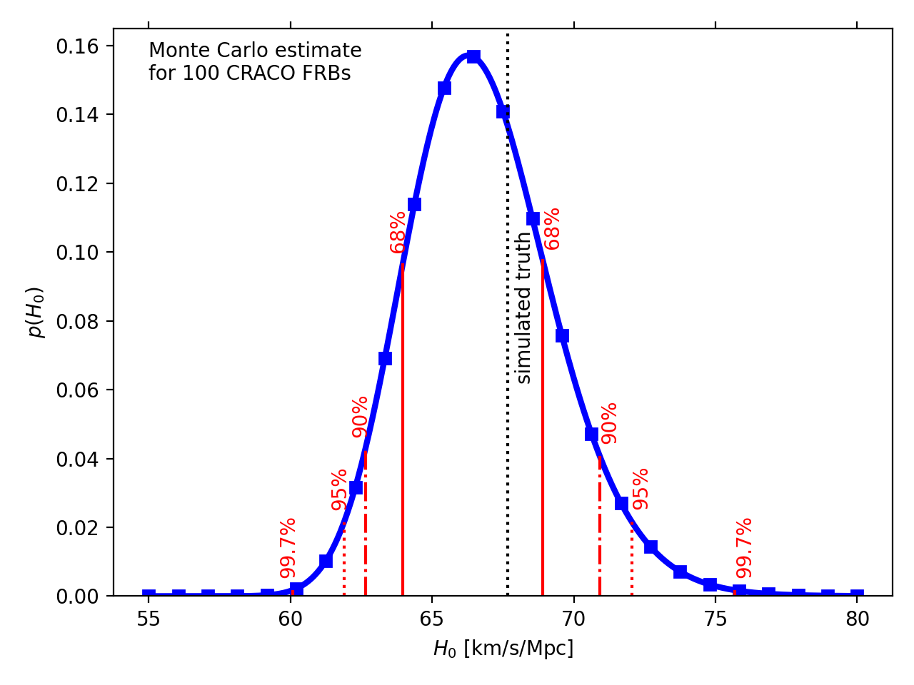
Figure 10: Posterior distribution on ${H_{0}}$ calculated from our Monte Carlo sample of 100 simulated FRBs that would be detected by the ASKAP CRACO upgrade (blue). Also shown are confidence intervals (red; labelled), and the simulated true value (black vertical line). Results with a uniform and Gaussian prior on $\alpha$ are indistinguishable.

Our limit on ${H_{0}}$ using the 16 localised and 60 unlocalised FRBs is not sufficiently constraining to discriminate between direct measurements from the local Universe and indirect measurements from the early Universe. However, in the near future, several experiments promise to greatly increase the number of localised FRBs. In particular, CRACO aims to implement a fully coherent image-plane FRB search during 2022.. The searches will be undertaken commensally with all other ASKAP observations.

We model CRACO by assuming $N_{\rm ant}=24$ of ASKAP’s 36 antennas are coherently added over a $\Delta\nu=288$ MHz bandwidth. Scaling the 22 Jy ms detection threshold to a 1 ms burst of the $\Delta\nu=336$ MHz Fly’s Eye survey (James et al., 2019a) by $N_{\rm ant}^{-1}(\Delta\nu)^{-0.5}$ gives an estimated detection threshold of $F_{\rm th}=0.99$ Jy ms. Assuming a Euclidean dependence of the FRB rate on sensitivity (i.e. $R\propto F_{\rm th}^{1.5}$), the Fly’s Eye rate of 20 FRBs in 1427 antenna days of observing predicts a 100-fold rate increase to 1.5 FRBs/day at high Galactic latitudes. This is then reduced by telescope down-time, RFI, time spent observing in the Galactic plane, and other efficiency losses in both radio observing and optical follow-up observations to identify host galaxies. Here, we use 100 FRBs to nominally represent the first year’s worth of CRACO observations. These FRBs are listed in Table 6, since they may be useful for other CRACO-related predictions, e.g. for gauging the requirements of optical follow-up observations.

We draw parameters $s$, DM, and $z$ randomly from the simulated distribution of $P(z,{\rm DM},\rm SNR)$  assuming Monte Carlo truth values of ${H_{0}}=67.66$ $\rm km\,s^{-1}\,Mpc^{-1}$and best-fit FRB population parameters from James et al. (2022b). These FRBs are plotted in Figure 2 and listed in Table 6. We repeat our calculation of $P(z,{\rm DM},\rm SNR)$ over the multidimensional grid of parameters given in Table 4, albeit limiting this to a more constrained range of ${H_{0}}$. The resulting Bayesian posterior probability distribution on ${H_{0}}$ is given in Figure 10.

For this particular FRB sample, we find ${H_{0}}=66.28_{-2.3}^{+2.6}$ $\rm km\,s^{-1}\,Mpc^{-1}$, consistent with the MC truth value of 67.66$\rm km\,s^{-1}\,Mpc^{-1}$. Importantly, the statistical uncertainty of $\sim 2.45$$\rm km\,s^{-1}\,Mpc^{-1}$— which includes the increased variance when fitting for FRB population parameters — would provide 2.5 $\sigma$ evidence to discriminate between the $\sim 6$  $\rm km\,s^{-1}\,Mpc^{-1}$ difference in estimates of ${H_{0}}$ (Abdalla et al., 2022). Assuming only statistical errors, to achieve $5\,\sigma$ discriminatory power would require 400 localised FRBs.

This suggests that near-future FRB observations — and perhaps only a single year’s worth of 100% efficient observations with the CRACO upgrade on ASKAP — will be able to help resolve the current discrepancy in the two measurements of ${H_{0}}$. It also motivates a careful treatment of potential systematic errors, both in the FRB sample used, and in the cosmological and FRB population model. We discuss such errors in §7.2.

Table 6: Monte Carlo FRBs generated for the (in development) CRACO system on ASKAP (see Section 6).

DM	${\rm SNR}$	$z$
	(${\rm pc\,cm^{-3}}$)
186.7	15.9	0.15
1179.5	26.0	1.321
438.5	20.2	0.062
315.3	17.9	0.089
833.1	10.5	0.949
595.3	32.8	0.25
313.4	16.8	0.37
568.5	13.1	0.629
143.5	11.0	0.026
743.4	12.6	0.812
941.9	10.0	0.755
460.5	10.7	0.355
1271.8	12.1	0.432
1308.6	15.7	1.273
567.9	12.4	0.608
410.5	84.7	0.057
391.1	117.3	0.251
1287.8	9.7	1.592
634.8	15.9	0.378
383.0	15.6	0.176
372.7	16.2	0.167
237.3	13.3	0.041
478.8	27.0	0.354
835.0	51.2	0.735
282.6	10.6	0.263
151.4	223.4	0.046
819.9	13.1	0.75
162.3	17.3	0.138
371.1	25.0	0.282
357.4	16.3	0.262
331.8	40.2	0.085
557.5	88.5	0.289
818.5	9.8	0.66
1257.6	22.4	0.699
1116.3	11.6	1.367
2259.2	12.3	1.338
307.9	22.6	0.243
1311.1	24.4	1.712
848.2	11.6	1.006
1060.6	10.6	1.108
785.5	10.0	0.164
484.9	11.7	0.52
481.2	9.6	0.424
484.7	14.9	0.61
260.6	12.9	0.054
393.8	12.7	0.291
273.7	22.7	0.182
534.4	21.0	0.556
703.6	10.8	0.195
335.9	18.5	0.329

DM	${\rm SNR}$	$z$
	(${\rm pc\,cm^{-3}}$)
898.1	32.2	0.718
582.2	13.8	0.571
636.2	23.1	0.441
735.7	27.7	0.482
1405.0	11.4	1.318
1083.0	19.3	1.101
709.4	12.4	0.58
1794.1	14.9	1.849
736.2	11.0	0.546
808.6	33.4	0.472
352.0	16.0	0.126
447.5	38.3	0.543
1346.2	12.3	1.567
428.3	12.3	0.537
421.8	28.0	0.018
602.3	16.3	0.093
1110.1	94.0	0.439
303.5	10.8	0.137
799.7	18.8	0.465
309.6	30.0	0.159
3446.6	25.6	0.08
721.5	25.8	0.306
296.3	21.4	0.134
573.2	19.6	0.464
184.5	11.4	0.063
580.0	15.6	0.632
754.0	9.6	0.103
391.9	11.2	0.43
282.0	21.7	0.073
548.7	25.8	0.35
449.7	12.6	0.019
187.9	40.8	0.052
522.1	11.8	0.353
233.3	85.5	0.081
923.9	9.9	0.961
568.1	15.9	0.295
1327.1	18.6	0.437
901.0	39.8	0.744
776.9	14.5	0.786
359.8	46.4	0.372
733.7	18.7	0.633
685.6	9.8	0.765
568.9	14.8	0.644
398.7	23.3	0.239
664.2	15.8	0.495
326.6	14.2	0.251
726.0	23.7	0.089
342.1	48.2	0.029
376.5	47.9	0.279
271.9	18.9	0.237

7 Discussion

7.1 Comparison to other estimates of ${H_{0}}$ with FRBs

Both Wu et al. (2022) (Wu22) and Hagstotz et al. (2022) (HS22) use measurements of FRBs to constrain ${H_{0}}$, finding ${H_{0}}$$=68.8^{+5.0}_{-4.3}$ $\rm km\,s^{-1}\,Mpc^{-1}$ and ${H_{0}}$$=62.3\pm 9.1$ $\rm km\,s^{-1}\,Mpc^{-1}$ respectively. These values are compatible at the $1\sigma$ level with our result of $73_{-8}^{+12}$ $\rm km\,s^{-1}\,Mpc^{-1}$ — however, it is still useful to analyse differences in the methods, especially given that common data was used.

Wu22 and HS22 use 18 and 9 localised FRBs respectively, in both cases including a subset of the bursts used in this analysis, and those from other instruments. These include repeating FRBs which have been localised purely because they are repeaters, which presents a biased distribution of the underlying population (Gardenier et al., 2019), although the effect of this bias is difficult to determine. Furthermore, neither study accounts for observational biases against high DMs, which will systematically increase ${H_{0}}$ by assuming the artificially low measured mean DMs reflect the true underlying distribution.

Both Wu22 and HS22 model DM contributions according to (1)–(3), with Wu22 in particular using very similar functional forms. HS22 however uses Gaussian distributions in linear space to model both ${\rm DM}_{\rm host}$ and ${\rm DM}_{\rm cosmic}$; given that they are symmetric about the mean, they do not include the high-DM tail, nor the relatively sharp lower limit to DM for a given redshift, expected for ${\rm DM}_{\rm EG}$.

Importantly, both Wu22 and HS22 allow for an uncertainty in ${\rm DM}_{\rm local}$, using $\sigma_{\rm MW}=30$ ${\rm pc\,cm^{-3}}$, with Wu22 also allowing ${\rm DM}_{\rm halo}$ to vary in the range 50–80 ${\rm pc\,cm^{-3}}$. Allowing for such uncertainties is an important next step in our model, due to the influence of the cliff effect.

Neither Wu22 nor HS22 however allow assumed values for other parameters in their model to vary — and ${H_{0}}$ is particularly sensitive to the assumed value of $\mu_{\rm host}$ (see Figure 9). HS22 assumes $\mu_{\rm host}$=100${\rm pc\,cm^{-3}}$, while Wu22 use a model for $\mu_{\rm host}$ based on the simulations of Zhang et al. (2020), with $\mu_{\rm host}$ increasing with $z$, and varying according to the class of FRB host galaxy (see discussion below). However, all values of $\mu_{\rm host}$ are lower than our best-fit median value of $10^{\mu_{\rm host}}=186$ ${\rm pc\,cm^{-3}}$. Since their assumed values are low, their assumed ${\rm DM}_{\rm IGM}$ will be increased, which we attribute as being primarily responsible for the lower ${H_{0}}$ values estimated by these authors.

7.2 Sources of Uncertainty and Bias

In this analysis, we have not allowed for uncertainties in the cosmological parameters $f_{d}(z)$, $\Omega_{b}h^{2}$, and the feedback parameter $F$. Of these, the current experimental uncertainty in $\Omega_{b}h^{2}$ is $\mathcal{O}\sim 0.5$% (Mossa et al., 2020a), and negligible compared to errors in the current calculation. In the future, we will need to marginalise over this uncertainty.

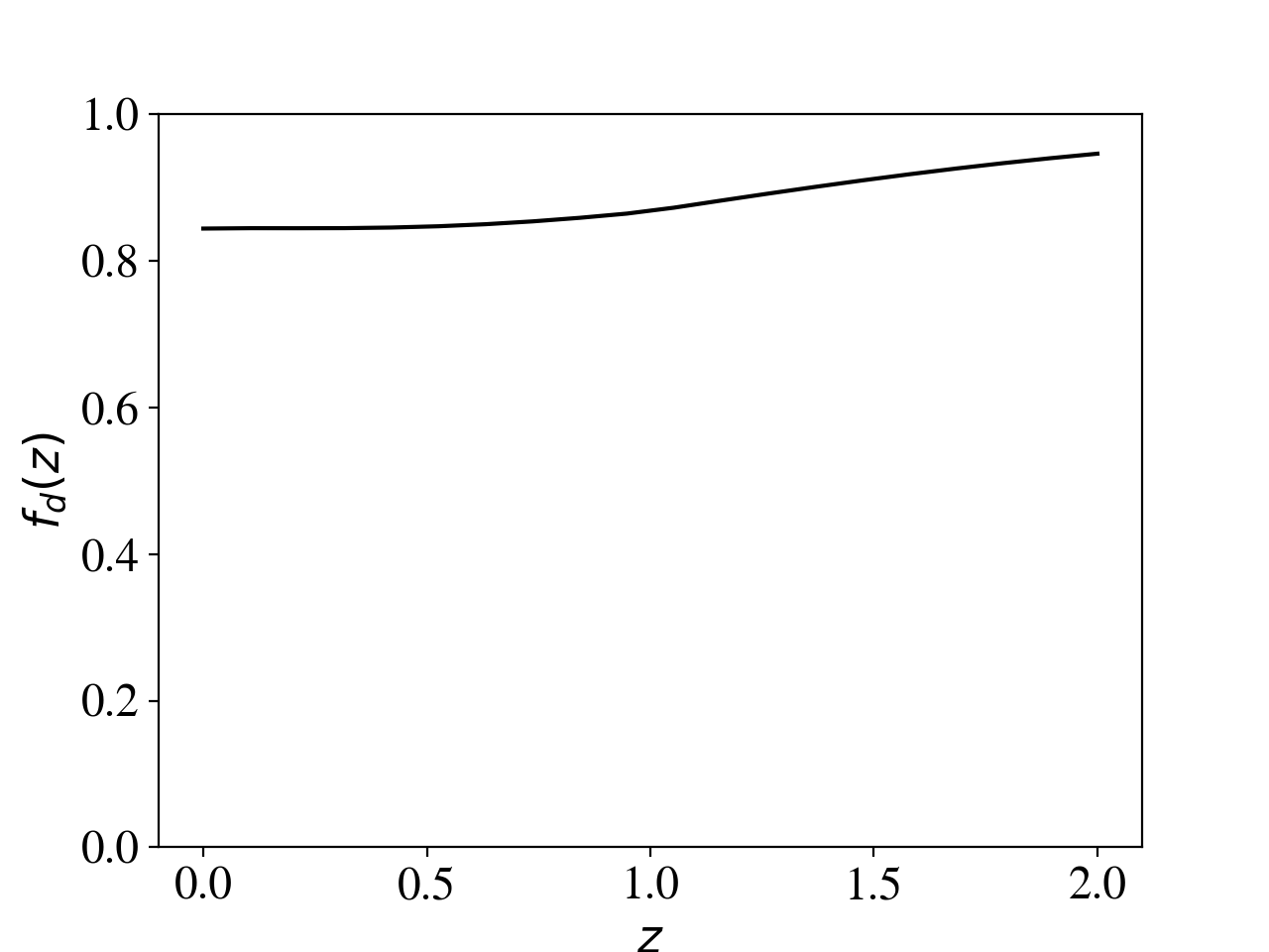
Figure 11: Modelled redshift evolution of the fraction of baryons that are diffused and ionized, $f_{d}(z)$, calculated according to Macquart et al. (2020) using code from Prochaska et al. (2019a).

Our adopted estimate for the fraction of baryons that are diffuse and ionized, $f_{d}(z)$, follows the methodology introduced in Prochaska et al. (2019a), and discussed in further detail in Macquart et al. (2020). The approach uses the estimated mass density of baryons in dense (i.e. neutral) gas and compact objects (stars, stellar remnants) from observations and stellar population modelling. For the present-day, one recovers $f_{d}(z=0)=0.844$ using the Planck Collaboration et al. (2020) parameters to estimate the total mass density in baryons. The redshift evolution of $f_{d}(z)$ is plotted in Figure 11. Regarding uncertainty in $f_{d}(z)$, the stellar mass estimate dominates primarily through our imprecise knowledge of the stellar initial mass function (IMF). If we assume a $30\%$ uncertainty in the stellar mass density (and associated remnants), this translates to a $4\%$ uncertainty in $f_{d}(z=0)$. As the statistical power of the FRB sample grows, this systematic error in $f_{d}(z)$ will rise in importance for ${H_{0}}$ analysis. It is possible, however, that upcoming experiments including weak-lensing surveys will reduce the IMF uncertainties. We also emphasize that at higher redshifts, $f_{d}$ increases as the masses of galaxies decreases. For example, a $30\%$ error in the stellar mass contribution at $z=1$ leads to a $\approx 2.5\%$ error in $f_{d}(z=1)$. In this respect, by including FRBs at $z>1$ one can partially alleviate the uncertainty in $f_{d}(z)$.

The feedback parameter $F$ acts to smear the distribution of ${\rm DM}_{\rm IGM}$ about the mean, with smaller values representing a larger ‘feedback’ effect that reduces the gas content of galactic halos, and hence a less clumpy Universe with a less smeared distribution of ${\rm DM}_{\rm IGM}$ (Cen & Ostriker, 2006). To first order, the influence of $F$ is similar to the smearing of ${\rm DM}_{\rm host}$ by $\sigma_{\rm host}$. Since both contribute to variance in ${\rm DM}_{\rm EG}$, and we fit $\sigma_{\rm host}$ to this, first-order uncertainties in $F$ are absorbed into $\sigma_{\rm host}$. However, variance in ${\rm DM}_{\rm EG}$ due to ${\rm DM}_{\rm host}$ is modelled as decreasing with $z$, while the absolute variance in ${\rm DM}_{\rm IGM}$ (due to $F$) increases with $z$. However, for future FRB samples — particularly those including localisations at $z\gtrsim 1$ — these terms should be separated, and $F$ explicitly fitted. For now, we note that $\sigma_{\rm host}$ and ${H_{0}}$ do show significant (anti-)correlation, and thus potentially errors in our (somewhat arbitrarily) adopted value of $F=0.32$ could influence our measurement of ${H_{0}}$, although we expect that the main effect of such an error is to shift the fitted value of $\sigma_{\rm host}$.

Related to this, we have used a fixed functional form for ${\rm DM}_{\rm host}$, which while allowing for the reduced DM due to redshift, does not allow for evolution of the host galaxy properties themselves. Indeed, our adopted log-normal distribution is not theoretically motivated, but rather is a qualitatively good description of the expected high-DM tail of ${\rm DM}_{\rm host}$. An improved model, including redshift evolution, will likely require combining FRB host galaxy studies (e.g. Bhandari et al., 2022) to derive empirical correlations similar to treatments of Hubble residuals with supernovae (e.g. Phillips, 1993). For instance, Zhang et al. (2020) find a cosmic evolution of $\mu_{\rm host}=C_{\rm DM}(1+z)^{\alpha_{\rm DM}}$, with constant $33\leq C_{\rm DM}\leq 96$ ${\rm pc\,cm^{-3}}$ and $0.83\leq\alpha_{\rm DM}\leq 1.08$, depending on galaxy type. Thus, when including the $(1+z)^{-1}$ redshift penalty to ${\rm DM}_{\rm host}$, the observed distribution of ${\rm DM}_{\rm host}$ should remain almost constant with redshift. Since $C_{\rm DM}$ varies with galaxy type however, so that the distribution of galaxy types — and thus presumably FRB host galaxies and thus $\mu_{\rm host}$ — will also vary with redshift. We suggest this topic for future investigations.

‘${\rm DM}_{\rm host}$’ represents all contributions to DM that come from the FRB occurring in a non-random part of the Universe, and thus includes the local cosmic structure (e.g. filament), halo, and interstellar medium of the host, and the immediate environment of the progenitor. Improvements in modelling should target all these aspects. One path forward is to use optical observations of the FRB host galaxy environment and intervening matter (Lee et al., 2022b), combined with properties such as the rotation measure and scattering of the FRB itself (Cordes et al., 2022), to constrain these values on a per-FRB basis.

Finally, we note that our models for the FRB luminosity function, and spectral behaviour, are relatively simplistic — the true behaviour is likely more complicated. These are discussed in more detail in J22a, and both can be investigated through near-Universe observations of FRBs.

7.3 Comparison with other methods

It is interesting to compare and contrast FRBs with other probes of ${H_{0}}$ in the local Universe. The traditional method of using Type Ia Supernovae (SNIa) relies on these being calibratable standard candles, using the cosmological distance ladder and in particular Cepheid variables (e.g. Riess et al., 2021, and references therein). This is certainly not the case for FRBs, which show a vast range of luminosity (Spitler et al., 2014; Shannon et al., 2018). However, using early Universe constraints on $\Omega_{b}h^{2}$ allows FRB DM to effectively become a ‘standard candle’, directly relating the value of DM to distance via the Macquart relation. This means however that FRB measures of ${H_{0}}$ in the local Universe will not be fully independent of early Universe cosmological fits, but can nonetheless be used to identify an inconsistent cosmology.

Both methods suffer from potential biases due to a changing nature of host galaxies with redshift, and concerns regarding dust extinction biases in SNIa (see e.g. Sullivan et al., 2003) are analogous to FRB detection biases against high DMs induced by FRB host galaxies. As discussed above, FRBs are sensitive to local Universe contributions to DM, which are less well-known than Galactic extinction effects on SN1a. Thus in many ways, FRB determination of ${H_{0}}$ is qualitatively similar to, but independent of, measures derived from SNIa — making them a perfect method for determining if the current Hubble tension is a result of systematic errors in the distance ladder, or a sign of new cosmology beyond $\Lambda$CDM.

Current limits on ${H_{0}}$ from FRBs are much less accurate than those from SNIa, with statistical errors of ${}_{-8}^{+12}$ $\rm km\,s^{-1}\,Mpc^{-1}$ compared to $\pm 1.01$ $\rm km\,s^{-1}\,Mpc^{-1}$ for SN1a (Riess et al., 2021). New experiments promise to dramatically increase the rate of both samples — the Legacy Survey of Space and Time (LSST) to be performed by the Rubin Observatory is expected to detect 400,000 Type Ia supernovae (Ivezić et al., 2019), while CRACO, DSA2000 (Hallinan et al., 2022), and CHORD (Vanderlinde et al., 2019) expect to increase the number of localised FRBs to the tens of thousands, although making use of this sample will require significant investment on optical telescopes to obtain host redshifts.

Gravitational wave (GW) detections also promise to constrain ${H_{0}}$ (Schutz, 1986). Since the intrinsic signal strength is precisely predicted from general relativity, there is essentially no calibration uncertainty. The challenge however lies in the event rate of localisable GW signals, which is very low, with so-far only a single event yielding an uncertainty of $70.3_{-5.0}^{+5.3}$ $\rm km\,s^{-1}\,Mpc^{-1}$ (Hotokezaka et al., 2019). There are also only moderate improvements expected in the near future (Abbott et al., 2020): a 1.8% precision on ${H_{0}}$ would require 50-100 binary neutron star (BNS) mergers with host galaxies, or 15 which also have afterglow information constraining their inclination angle (Hotokezaka et al., 2019). The expected rate of BNS detection during the upcoming fourth observing run (‘O4’) of the LIGO–Virgo–KAGRA GW detectors, at $7.7^{+11.9}_{-5.7}$ yr^-1, is too uncertain to make hard predictions about the time required to reach these numbers (Colombo et al., 2022). The $\sim 78\%$ fraction of these events that will produce a kilonova (and hence redshift via host galaxy identification), and $\sim 10\%$ fraction that will produce a detectable jet constraining their inclination angle, must also be considered (Colombo et al., 2022).

Therefore, provided that the systematic errors discussed in Section 7.2 can be reduced, FRBs will be a valuable cosmological probe, should be at least as precise as GW-based approaches, and have the potential to approach SN1a in precision.

8 Conclusions

Using a sample of 16 localised and 60 unlocalised FRBs, we have fitted the observed values of ${\rm SNR}$, $z$, and DM for each FRB, and the number of FRBs observed by each survey, using a Bayesian approach. We use the methodology of James et al. (2022a), which includes the biasing effects of telescope beamshape and the FRB width, and models the FRB luminosity function, source evolution, and properties of the FRB population and their host galaxies. We have updated the method to allow ${H_{0}}$ to vary while adjusting $\Omega_{b}$ according to precise constraints on $\Omega_{b}h^{2}$ from the CMB. We find a best-fit value of $73_{-8}^{+12}$ $\rm km\,s^{-1}\,Mpc^{-1}$, consistent with both direct and indirect measures of ${H_{0}}$ (Abdalla et al., 2022), and other estimates using FRBs (Wu et al., 2022; Hagstotz et al., 2022). This estimate was obtained with uniform priors over the entire range of $\mu_{\rm host}$, $\sigma_{\rm host}$, $\log_{10}E_{\rm max}$, $\gamma$, and $n_{\rm sfr}$ where the likelihood is non-vanishing; and the plausible range of $-2\leq\alpha\leq 0$ allowed by other studies.

We discuss systematic differences in the different methodologies for inferring ${H_{0}}$ from FRB samples, and we attribute the lower values of ${H_{0}}$ found by those studies to be primarily due to their low assumed values of ${\rm DM}_{\rm host}$, which we fit, finding a median host contribution of $186^{+59}_{-48}$ ${\rm pc\,cm^{-3}}$ (from an assumed Galactic halo contribution of ${\rm DM}_{\rm halo}=50\,{\rm pc\,cm^{-3}}$).

The addition of new data confirms the previous result of James et al. (2022b) that the FRB population evolves with redshift in a manner consistent with the star-formation rate, and excludes no source evolution at $3\,\sigma$. This is consistent with young magnetar scenarios, and the presence of FRBs near spiral arms Mannings et al. (2021), although we do not specifically exclude older progenitors. We have also constrained the frequency dependence of the FRB rate, albeit weakly, finding that $R_{\rm FRB}\propto\nu^{-1\pm 0.85}$. Our estimated slope of the cumulative luminosity function is $\gamma=-0.95_{-0.15}^{+0.18}$, slightly flatter than previous estimates, and consistent with values derived from individual repeating FRBs.

We have used Monte Carlo simulations to predict that 100 localised FRBs from the first year of operation of the CRACO system of ASKAP will be able to constrain ${H_{0}}$ with a statistical uncertainty of $\approx\pm 2.45\rm km\,s^{-1}\,Mpc^{-1}$, giving significant power to discriminate between different existing estimates. This motivates further work to address systematic uncertainties in our modelling, in particular to constrain or fit the fraction of cosmic baryons in diffuse ionized gas, and the contribution of the Milky Way halo to DM.

Data Availability

The code used in this study is available from GitHub (Prochaska et al., 2019a; James et al., 2021), which also includes the input FRB data. The calculated values of $P(N_{\rm FRB})$ and $P(z,{\rm DM},\rm SNR)$ for each dataset takes up several GB, and a download link is available upon request to the authors.

Appendix A Studies of systematic effects

In this Appendix, we present several studies of potential systematic effects which, if not properly controlled, could bias our estimates of ${H_{0}}$.

A.1 Missing low-${\rm SNR}$ FRBs

The question of completeness in FRB surveys has been discussed by several authors (e.g. Macquart & Ekers, 2018a; Bhandari et al., 2018; James et al., 2019b). From a simulation perspective, we assume completeness above some signal-to-noise threshold, ${\rm SNR}_{\rm th}$, i.e. all FRBs with ${\rm SNR}_{\rm FRB}>{\rm SNR}_{\rm th}$ are detected. However, practically, this may not be case. FRBs which pass the threshold are usually required to be either visually inspected, and/or analysed by an algorithm, to distinguish these events from RFI. Such an inspection — whether done by human or machine — will be more likely to fail for weak FRBs than for strong ones. This observational bias has been suggested as one reason why the first FRB to be discovered, the ‘Lorimer burst’ (FRB 20010724; Lorimer et al., 2007), was exceptionally bright — because all the other bursts which had been viewed, but were not so bright, had not been identified (Macquart & Ekers, 2018a). It has also been suggested to explain the dearth of Parkes FRBs with ${\rm SNR}<14$, although there is no evidence of such a bias from the CRAFT/FE observations (James et al., 2019c).

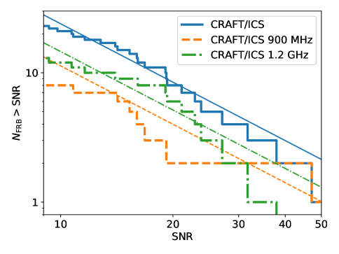
Figure 12: Cumulative event count as a function of FRB SNR for all CRAFT/ICS observations (blue, solid), and separated into CRAFT/ICS $900\,{\rm MHz}$ (orange, dashed) and CRAFT/ICS $1.3\,{\rm GHz}$ (green, dot-dash). Only two CRAFT/ICS $1.6\,{\rm GHz}$ FRBs were detected and are not shown separately. Also shown are fits to a ${\rm SNR}^{-1.5}$ power law.

For CRAFT/ICS observations, the detection threshold, ${\rm SNR}_{\rm th}$, initially had to be set as high as 14$\sigma$ to reduce the number of false RFI candidates. Subsequently, an improved clustering algorithm, snoopy2, was developed to analyse all events satisfying ${\rm SNR}_{\rm FRB}>{\rm SNR}_{\rm th}$ and reject RFI. This algorithm has been shown to pass all FRBs detected in ASKAP/FE observations. Furthermore, ASKAP/ICS observations of pulsars have not shown any evidence of behaviour that would reject true FRBs, i.e. all pulsar pulses above the detection threshold are not rejected. Thus CRAFT/ICS observations typically use a threshold of 9$\sigma$.

Figure 12 plots the number of ASKAP FRBs observed above different ${\rm SNR}$ values. In a Euclidean Universe, this logN–logS curve should have a power-law slope of -1.5. However, for CRAFT/ICS, there is evidence for an inflection point near ${\rm SNR}$ of 15. While part of this inflection can be explained by early observations with a high ${\rm SNR}_{\rm th}$, the threshold had stablised by the time of the 900 MHz observations — and the inflection point is present at both frequency ranges.

The source of this deficit of low-${\rm SNR}$ FRBs is unknown. One potential solution is to artificially increase the detection threshold to an ${\rm SNR}$ of 15, and to discard all FRBs with ${\rm SNR}<15$. Before discarding valuable events however, we first investigate the potential bias of including FRBs in the range $9.5<{\rm SNR}<15$.

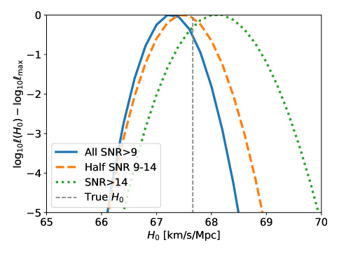
Figure 13: Simulated sensitivity to ${H_{0}}$ of CRAFT/ICS $1.3\,{\rm GHz}$ observations when using all events with ${\rm SNR}\geq 9$, excluding half in the range $9\leq{\rm SNR}<14$, and only using events with ${\rm SNR}\geq 14$.

To do so, we simulate 1000 FRBs from CRAFT/ICS $1.3\,{\rm GHz}$ using ${\rm SNR}_{\rm th}=9$, and calculate the likelihood $\ell$(${H_{0}}$) while holding all other parameters constant. As this is a single survey, $P(N_{\rm FRB})$ has no contribution, since the population density can always be appropriately scaled. The result is shown in Figure 13. We then repeat the calculation by randomly removing half of all FRBs in the range $9\leq{\rm SNR}\leq 14$ while keeping ${\rm SNR}_{\rm th}=9$ as in the main analysis, and by removing all FRBs with ${\rm SNR}<15$ but accounting for this via setting ${\rm SNR}_{\rm th}=15$. Thus both ${\rm SNR}>9$ and ${\rm SNR}>14$ calculations should present unbiased (but statistically fluctuating) measures of ${H_{0}}$, while the ‘half SNR 9–14’ sample will present a biased estimate.

In Figure 13, the unbiased samples correctly reproduce the simulated true value of ${H_{0}}$ with errors of $\pm 0.5$ $\rm km\,s^{-1}\,Mpc^{-1}$. The biased half 9–14 sample produces ${H_{0}}$ in-between these two values — very close to the simulated truth. Thus while we cannot exclude that missing FRBs in the range $9\leq{\rm SNR}\leq 14$ results in a bias, this bias is smaller than the random deviation in ${H_{0}}$ when using 1000 FRBs. Therefore we include the six FRBs with $9\leq{\rm SNR}\leq 14$ in our sample, and use ${\rm SNR}_{\rm th}=9$; and we suggest that all near-future FRB surveys do the same.

A.2 Effect of ISM

The Milky Way interstellar medium (ISM) increases the dispersion measure of extragalactic FRBs at low Galactic latitudes through an increasing ${\rm DM}_{\rm ISM}$. This in turn reduces the sensitivity of FRB surveys at these latitudes in terms of extragalactic dispersion measure, ${\rm DM}_{\rm EG}$. Whether or not the apparent paucity of FRBs observed at low Galactic latitudes by Parkes (Petroff et al., 2014) is due to this effect or e.g. interstellar scintillation (Macquart & Johnston, 2015), or is indeed even statistically significant (Bhandari et al., 2018), remains undetermined. Here, we model the effects of ${\rm DM}_{\rm ISM}$ on the redshift distribution $z$ of observable FRBs using CRAFT/ICS $1.3\,{\rm GHz}$. Note that the Galactic Plane also reduces the ability of optical follow-up observations to identify the FRB host galaxy, as discussed in §4.5. Here we only consider only the effects on the initial detection of FRBs with radio waves.

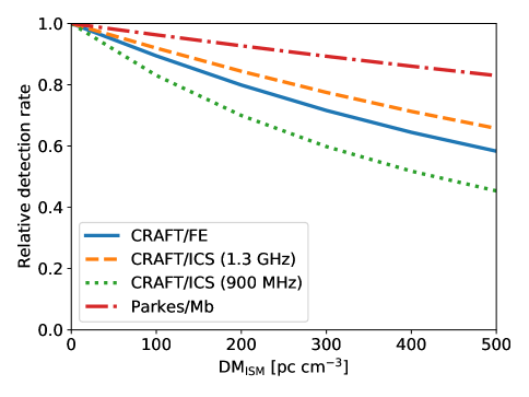
Figure 14: Dependence of total FRB detection rate on ${\rm DM}_{\rm ISM}$, relative to the hypothetical rate when ${\rm DM}_{\rm ISM}$$=0$.

In Figure 14, we plot the total (simulated) detectable FRB rate as a function of ${\rm DM}_{\rm ISM}$ for the FRB surveys used in this work. In the range of 0–500 ${\rm pc}\,{\rm cm}^{-3}$, the detection rate falls the least ($\sim$20%) for Parkes/Mb, due to its high frequency resolution negating the effects of increased DM smearing; and the most ($\sim$50%) for CRAFT/ICS $900\,{\rm MHz}$ due to its lower observation frequency and hence greater DM smearing.

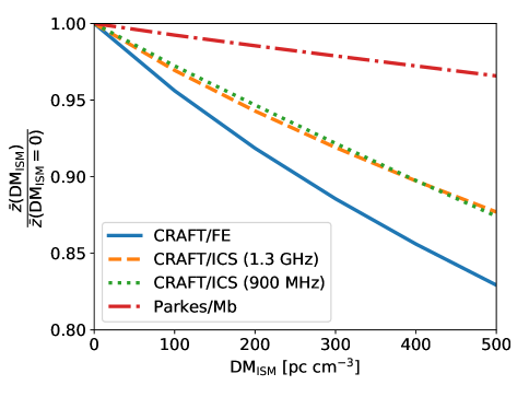
Figure 15: Dependence of mean detected redshift $z$ on ${\rm DM}_{\rm ISM}$.

The effect of this reduced sensitivity on the observable redshift distribution is shown in Figure 15. An increased ${\rm DM}_{\rm ISM}$ decreases the mean redshift of detectable FRBs, $\bar{z}$, for all surveys considered here. Again, Parkes/Mb is the least affected survey. However, the relative effect on CRAFT/FE (17% reduction in $\bar{z}$ at ${\rm DM}_{\rm ISM}=500{\rm pc}\,{\rm cm}^{-3}$ relative to ${\rm DM}_{\rm ISM}=0{\rm pc}\,{\rm cm}^{-3}$) is now greater than that on CRAFT/ICS $900\,{\rm MHz}$. This is likely because the lower sensitivity of CRAFT/FE leads to, on-average, lower values of ${\rm DM}_{\rm EG}$, so that a moderate increase in ${\rm DM}_{\rm ISM}$ has a proportionally greater effect on sensitivity and hence $\bar{z}$.

To test the effect of this approximation on ${H_{0}}$, we use simulated FRBs from CRAFT/ICS $1.3\,{\rm GHz}$ and the best-fit parameters of James et al. (2022b). We simulate four sets of FRBs, setting ${\rm DM}_{\rm ISM}$to $0$, $100$, $200$, and $500$ ${\rm pc}\,{\rm cm}^{-3}$. To illustrate the bias effect of ${\rm DM}_{\rm ISM}$ on ${H_{0}}$, we evaluate the likelihood $\ell$ by changing ${H_{0}}$ only, subject to the constraint on $\Omega_{b}h^{2}$.

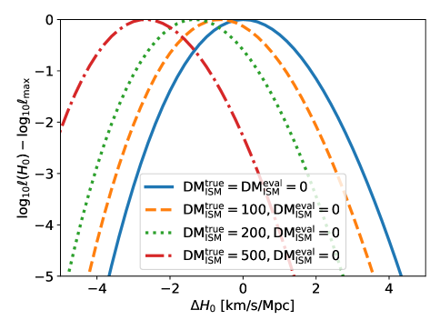
Figure 16: Effect on evaluated likelihoods of ${H_{0}}$ (relative to maximum) when using an incorrect value of ${\rm DM}_{\rm ISM}$ for evaluation.

For our first test, we use samples of FRBs with ${\rm DM}_{\rm EG}$ generated at true values of ${\rm DM}_{\rm ISM}$, ${\rm DM}_{\rm ISM}^{\rm true}$, of $0$, $100$, $200$, and $500$ ${\rm pc}\,{\rm cm}^{-3}$, but ${H_{0}}$ is evaluated assuming a different value, ${\rm DM}_{\rm ISM}^{\rm eval}=0$. The results are shown in Figure 16. In all cases, the most likely value of ${H_{0}}$ is evaluated as being lower, by 0.6, 1.4, and 2.6 $\rm km\,s^{-1}\,Mpc^{-1}$for $100$, $200$, and $500$ ${\rm pc}\,{\rm cm}^{-3}$respectively, to account for seeing FRBs with lower ${\rm DM}_{\rm FRB}$ for a given redshift.

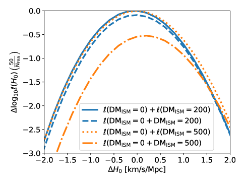
Figure 17: Effect of merging samples with common ${\rm DM}_{\rm ISM}$ on $H_{0}$.

The effect of ${\rm DM}_{\rm ISM}$ on ${H_{0}}$ illustrated in Figure 16 is accounted-for in our simulation code, by subtracting ${\rm DM}_{\rm ISM}$ (and ${\rm DM}_{\rm host}$) from ${\rm DM}_{\rm FRB}$ to calculate ${\rm DM}_{\rm EG}$ on a per-event basis. However, the observation bias as a function of ${\rm DM}_{\rm EG}$ is calculated using the mean value of ${\rm DM}_{\rm ISM}$ for each sample only. This is done purely because generating a $z$–DM grid for each FRB individually is too computationally expensive.

To test the effect of mixing FRBs with different values of ${\rm DM}_{\rm ISM}$ into the same evaluation, we take samples of FRBs generated at ${\rm DM}_{\rm ISM}=200$ and $500$ ${\rm pc}\,{\rm cm}^{-3}$, and add them to the sample generated at ${\rm DM}_{\rm ISM}=0$ ${\rm pc}\,{\rm cm}^{-3}$. ${H_{0}}$ is then evaluated using the default method of averaging ${\rm DM}_{\rm ISM}$ over the sample, i.e. to ${\rm DM}_{\rm ISM}=100$ and ${\rm DM}_{\rm ISM}=250$ ${\rm pc}\,{\rm cm}^{-3}$ respectively. This is compared to results on ${H_{0}}$ generated by treating samples at ${\rm DM}_{\rm ISM}=0$, $200$, and $500$ ${\rm pc}\,{\rm cm}^{-3}$ individually, i.e. such that the average value of ${\rm DM}_{\rm ISM}$ is the correct one. Results are shown in Figure 17, giving the shift in most likely value of ${H_{0}}$, and the change in maximum likelihood $\ell_{\rm max}$ per 50 events (the vertical shift in maximum likelihood over 2000 events can be quite large, and prevents easy display). The effect of averaging ${\rm DM}_{\rm ISM}$ over 0 and 200 ${\rm pc}\,{\rm cm}^{-3}$ is negligible, resulting in bias of only +0.027 $\rm km\,s^{-1}\,Mpc^{-1}$. Mixing samples of FRBs with ${\rm DM}_{\rm ISM}$ between 0 and 500 ${\rm pc}\,{\rm cm}^{-3}$ is less reliable, with a bias of 0.18 $\rm km\,s^{-1}\,Mpc^{-1}$.

These biases are currently significantly smaller than the random errors from our small sample of localised FRBs, especially given that all have been detected with ${\rm DM}_{\rm ISM}<200$ ${\rm pc}\,{\rm cm}^{-3}$. Thus we loosen the constraint of ${\rm DM}_{\rm ISM}<100$ ${\rm pc}\,{\rm cm}^{-3}$ previously adopted in James et al. (2022a), and include all FRBs localised by ASKAP in our main analysis. It also allows us to include ASKAP/FE and Parkes/Mb FRBs originally excluded from the sample of James et al. (2022a), which are listed in Table 3.

A.3 Effect of unlocalised ASKAP/ICS FRBs

The majority of ASKAP/ICS FRBs have had their host galaxies, and hence redshifts, identified. However, several FRBs remain unlocalised, as described in §4.5. These reasons generally fall into two categories: reasons uncorrelated with FRB properties, which result in reduced statistical power on ${H_{0}}$ but no potential bias; and those which are correlated with FRB properties, and thus could potentially bias a study such as that presented in this work.

In particular, the sample used in this work includes two FRBs with DM over 1000 ${\rm pc}\,{\rm cm}^{-3}$ (FRB 20210407 and FRB 20210912) with potentially high-redshift host galaxies which have not been identified in initial follow-up observations with the VLT, although in the former case Galactic extinction plays a significant role. If ${\rm DM}_{\rm FRB}$ is dominated by ${\rm DM}_{\rm cosmic}$ therefore, the hosts of these FRBs will lie at $z\gtrsim 1$ and may not be detectable with standard follow-up observations. However, if ${\rm DM}_{\rm FRB}$ is dominated by a large host contribution — such as FRB 20210117A (Bhandari et al. (in prep.))— the host will be readily identified. This then leads to a sample biased towards low redshift.

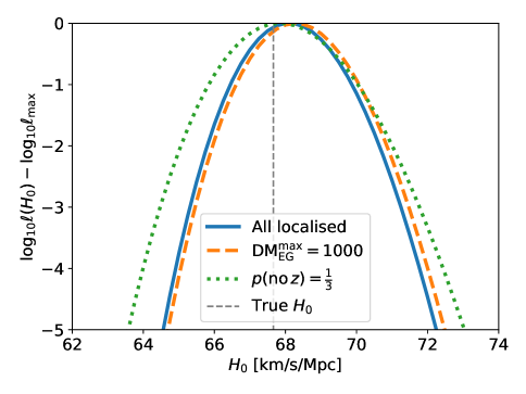
Figure 18: Constraints on ${H_{0}}$ obtained from 1000 synthetic (Monte Carlo) FRBs when varying ${H_{0}}$ only, assuming all bursts are localised; when discarding all 30 bursts with ${\rm DM}_{\rm EG}>{\rm DM}_{\rm EG}^{\rm max}=1000$ ${\rm pc}\,{\rm cm}^{-3}$; and when also discarding one third of FRBs chosen randomly. No bias is visible when estimating ${H_{0}}$, but some loss of accuracy is, as expected.

To counter this effect, we place an upper limit on ${\rm DM}_{\rm EG}$, ${\rm DM}_{\rm EG}^{\rm max}$, below which we expect all FRB hosts to be identifiable. Above ${\rm DM}_{\rm EG}^{\rm max}$, we discard all redshift information, even if known. We also include the DM of FRBs that remain unlocalised for observational reasons. This implementation has been tested using Monte Carlo FRBs generated from the CRAFT/ICS $1.3\,{\rm GHz}$ survey parameters, as per Appendix A.2. Results are shown in Figure 18. Clearly, the loss of information when removing FRB redshifts results in poorer statistical constraints on ${H_{0}}$ — however, no systematic bias has been introduced.

A.4 Effects of gridding in $z$–DM space

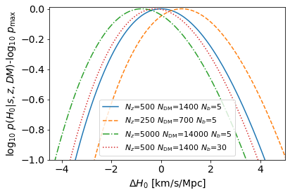
Figure 19: Simulated systematic effect on ${H_{0}}$ estimates using the CRACO due to the number of redshifts $N_{z}$, DMs $N_{\rm DM}$, and beam values $N_{b}$. Shown is the posterior probability distribution $\log_{10}p({H_{0}}|s,z,{\rm DM})$ normalised to the maximum value, as a function of $\Delta{H_{0}}$, i.e. the deviation from the best-fit value of ${H_{0}}$ obtained for the default grid of $N_{\rm DM}$=1400, $N_{z}$= 500 and $N_{b}$=5.

The probability distribution $P(z,{\rm DM})$ is calculated on a finite grid of $N_{z}=500$ linearly spaced redshifts up to $z=5$ and $N_{\rm DM}=1400$ linearly spaced dispersion measures up to $\rm{DM}=7000$ ${\rm pc}\,{\rm cm}^{-3}$. Furthermore, we parameterise the telescope beamshape using only $N_{b}=5$ combinations of beam sensitivity $B$ and solid angle $\Omega(B)$. To test the effects of this choice of gridding, we again calculate $p({H_{0}}|s,z,{\rm DM})$ for different gridding choices using the simulated CRACO sample while holding all other parameters fixed. The results are shown in Figure 19.

We find that our best-fitting value of ${H_{0}}$ varies by $\pm 1$$\rm km\,s^{-1}\,Mpc^{-1}$ according to our choice of gridding: for this particular sample, a grid sparser by a factor of two ($N_{z}=250$, $N_{\rm DM}=700$) produces a higher value of ${H_{0}}$ by 1 $\rm km\,s^{-1}\,Mpc^{-1}$, while ten-fold finer grid ($N_{z}=5000$, $N_{\rm DM}=14000$) produces a lower value of ${H_{0}}$ by 1 $\rm km\,s^{-1}\,Mpc^{-1}$. Increasing $N_{b}$ has almost no effect on the estimation of ${H_{0}}$, which is likely due to this parameter being extensively optimised by J22a.

We attribute this sensitivity to two regions of parameter space that are sensitive to smoothness, being the sharp decline in $P({\rm DM}|z)$ near the lower boundary due to the cliff effect, and the low-$z$ region.

Compared to our current uncertainty in ${H_{0}}$ estimates with FRBs, a potential systematic error of $\pm 1$ $\rm km\,s^{-1}\,Mpc^{-1}$ is small. However, in future, this suggests either using a finer grid in $z$–DM space; optimising the spacing, e.g. using log-spaced grids; or shifting to a method which does not use a brute force calculation over a grid, but performs a more intelligent optimisation of parameters.

References

- Abbott et al. (2020) Abbott B. P., et al., 2020, Living Reviews in Relativity, 23, 3
- Abdalla et al. (2022) Abdalla E., et al., 2022, arXiv e-prints, p. arXiv:2203.06142
- Aggarwal et al. (2021) Aggarwal K., Budavári T., Deller A. T., Eftekhari T., James C. W., Prochaska J. X., Tendulkar S. P., 2021, ApJ, 911, 95
- Arcus et al. (2021) Arcus W. R., Macquart J. P., Sammons M. W., James C. W., Ekers R. D., 2021, MNRAS, 501, 5319
- Aver et al. (2021) Aver E., Berg D. A., Olive K. A., Pogge R. W., Salzer J. J., Skillman E. D., 2021, J. Cosmology Astropart. Phys., 2021, 027
- Bannister et al. (2017) Bannister K. W., et al., 2017, ApJ, 841, L12
- Bannister et al. (2019) Bannister K. W., et al., 2019, Science, 365, 565
- Bhandari et al. (2018) Bhandari S., et al., 2018, MNRAS, 475, 1427
- Bhandari et al. (2020) Bhandari S., et al., 2020, ApJ, 901, L20
- Bhandari et al. (2022) Bhandari S., et al., 2022, AJ, 163, 69
- Bhat et al. (2004) Bhat N. D. R., Cordes J. M., Camilo F., Nice D. J., Lorimer D. R., 2004, ApJ, 605, 759
- Bhattacharyya et al. (2022) Bhattacharyya S., Tiwari H., Bharadwaj S., Majumdar S., 2022, MNRAS, 513, L1
- Burke-Spolaor & Bannister (2014) Burke-Spolaor S., Bannister K. W., 2014, ApJ, 792, 19
- CHIME/FRB Collaboration et al. (2021) CHIME/FRB Collaboration et al., 2021, ApJS, 257, 59
- Caleb et al. (2019) Caleb M., Flynn C., Stappers B. W., 2019, MNRAS, 485, 2281
- Cao et al. (2018) Cao X.-F., Yu Y.-W., Zhou X., 2018, ApJ, 858, 89
- Cen & Ostriker (2006) Cen R., Ostriker J. P., 2006, ApJ, 650, 560
- Chime/Frb Collaboration et al. (2020) Chime/Frb Collaboration et al., 2020, Nature, 582, 351
- Colombo et al. (2022) Colombo A., Salafia O. S., Gabrielli F., Ghirlanda G., Giacomazzo B., Perego A., Colpi M., 2022, arXiv e-prints, p. arXiv:2204.07592
- Connor (2019) Connor L., 2019, MNRAS, 487, 5753
- Cooke et al. (2018) Cooke R. J., Pettini M., Steidel C. C., 2018, ApJ, 855, 102
- Cordes & Lazio (2002) Cordes J. M., Lazio T. J. W., 2002, ArXiv Astrophysics e-prints,
- Cordes et al. (2022) Cordes J. M., Ocker S. K., Chatterjee S., 2022, ApJ, 931, 88
- Day et al. (2020) Day C. K., et al., 2020, MNRAS, 497, 3335
- Day et al. (2021) Day C. K., Deller A. T., James C. W., Lenc E., Bhandari S., Shannon R. M., Bannister K. W., 2021, Publ. Astron. Soc. Australia, 38, e050
- Eftekhari & Berger (2017) Eftekhari T., Berger E., 2017, ApJ, 849, 162
- Farah et al. (2019) Farah W., et al., 2019, MNRAS, 488, 2989
- Feldman & Cousins (1998) Feldman G. J., Cousins R. D., 1998, Phys. Rev. D, 57, 3873
- Freedman et al. (2001) Freedman W. L., et al., 2001, The Astrophysical Journal, 553, 47
- Gajjar et al. (2018) Gajjar V., et al., 2018, ApJ, 863, 2
- Gardenier et al. (2019) Gardenier D. W., van Leeuwen J., Connor L., Petroff E., 2019, A&A, 632, A125
- Hagstotz et al. (2022) Hagstotz S., Reischke R., Lilow R., 2022, MNRAS, 511, 662
- Hallinan et al. (2022) Hallinan G., Ravi V., Walter F., 2022, in American Astronomical Society Meeting Abstracts. p. 409.06
- Heintz et al. (2020) Heintz K. E., et al., 2020, ApJ, 903, 152
- Hessels et al. (2019) Hessels J. W. T., et al., 2019, ApJ, 876, L23
- Hewitt et al. (2022) Hewitt D. M., et al., 2022, MNRAS,
- Hotan et al. (2021) Hotan A. W., et al., 2021, Publ. Astron. Soc. Australia, 38, e009
- Hotokezaka et al. (2019) Hotokezaka K., Nakar E., Gottlieb O., Nissanke S., Masuda K., Hallinan G., Mooley K. P., Deller A. T., 2019, Nature Astronomy, 3, 940
- Hunter (2007) Hunter J. D., 2007, Computing in Science and Engineering, 9, 90
- Inoue (2004) Inoue S., 2004, MNRAS, 348, 999
- Ivezić et al. (2019) Ivezić Ž., et al., 2019, ApJ, 873, 111
- Jahns et al. (2022) Jahns J. N., et al., 2022, arXiv e-prints, p. arXiv:2202.05705
- James et al. (2019a) James C. W., et al., 2019a, Publ. Astron. Soc. Australia, 36, e009
- James et al. (2019b) James C. W., Ekers R. D., Macquart J.-P., Bannister K. W., Shannon R. M., 2019b, MNRAS, 483, 1342
- James et al. (2019c) James C. W., Ekers R. D., Macquart J. P., Bannister K. W., Shannon R. M., 2019c, MNRAS, 483, 1342
- James et al. (2021) James C. W., Prochaska J. X., Ghosh E. M., 2021, zdm, https://zenodo.org/record/5213780#.YRxh5BMzZKA
- James et al. (2022a) James C. W., Prochaska J. X., Macquart J. P., North-Hickey F. O., Bannister K. W., Dunning A., 2022a, MNRAS, 509, 4775
- James et al. (2022b) James C. W., Prochaska J. X., Macquart J. P., North-Hickey F. O., Bannister K. W., Dunning A., 2022b, MNRAS, 510, L18
- Keane et al. (2011) Keane E. F., Kramer M., Lyne A. G., Stappers B. W., McLaughlin M. A., 2011, MNRAS, 415, 3065
- Keane et al. (2016) Keane E., et al., 2016, Nature, 530, 453
- Keane et al. (2018) Keane E. F., et al., 2018, MNRAS, 473, 116
- Keating & Pen (2020) Keating L. C., Pen U.-L., 2020, MNRAS, 496, L106
- Lee et al. (2022a) Lee K.-G., Ata M., Khrykin I. S., Huang Y., Prochaska J. X., Cooke J., Zhang J., Batten A., 2022a, ApJ, 928, 9
- Lee et al. (2022b) Lee K.-G., Ata M., Khrykin I. S., Huang Y., Prochaska J. X., Cooke J., Zhang J., Batten A., 2022b, ApJ, 928, 9
- Lemos et al. (2022) Lemos T., Gonçalves R. S., Carvalho J. C., Alcaniz J. S., 2022, arXiv e-prints, p. arXiv:2205.07926
- Li et al. (2021) Li D., et al., 2021, Nature, 598, 267
- Locatelli et al. (2019) Locatelli N., Ronchi M., Ghirlanda G., Ghisellini G., 2019, A&A, 625, A109
- Lorimer et al. (2007) Lorimer D. R., Bailes M., McLaughlin M. A., Narkevic D. J., Crawford F., 2007, Science, 318, 777
- Macquart & Ekers (2018a) Macquart J.-P., Ekers R. D., 2018a, MNRAS, 474, 1900
- Macquart & Ekers (2018b) Macquart J.-P., Ekers R., 2018b, MNRAS, 480, 4211
- Macquart & Johnston (2015) Macquart J.-P., Johnston S., 2015, MNRAS, 451, 3278
- Macquart et al. (2019) Macquart J.-P., Shannon R. M., Bannister K. W., James C. W., Ekers R. D., Bunton J. D., 2019, ApJ, 872, L19
- Macquart et al. (2020) Macquart J. P., et al., 2020, Nature, 581, 391
- Madau & Dickinson (2014) Madau P., Dickinson M., 2014, ARA&A, 52, 415
- Madhavacheril et al. (2019) Madhavacheril M. S., Battaglia N., Smith K. M., Sievers J. L., 2019, Phys. Rev. D, 100, 103532
- Mannings et al. (2021) Mannings A. G., et al., 2021, ApJ, 917, 75
- Masui & Sigurdson (2015) Masui K. W., Sigurdson K., 2015, Phys. Rev. Lett., 115, 121301
- McQuinn (2014) McQuinn M., 2014, ApJ, 780, L33
- Metzger et al. (2017) Metzger B. D., Berger E., Margalit B., 2017, ApJ, 841, 14
- Mossa et al. (2020a) Mossa V., et al., 2020a, Nature, 587, 210
- Mossa et al. (2020b) Mossa V., et al., 2020b, Nature, 587, 210
- Niu et al. (2022) Niu C. H., et al., 2022, Nature, 606, 873
- Osłowski et al. (2019) Osłowski S., et al., 2019, MNRAS, 488, 868
- Petroff et al. (2014) Petroff E., et al., 2014, ApJL, 789, L26
- Petroff et al. (2017) Petroff E., et al., 2017, MNRAS, 469, 4465
- Phillips (1993) Phillips M. M., 1993, ApJ, 413, L105
- Planck Collaboration et al. (2020) Planck Collaboration et al., 2020, A&A, 641, A6
- Platts et al. (2019) Platts E., Weltman A., Walters A., Tendulkar S. P., Gordin J. E. B., Kandhai S., 2019, Phys. Rep., 821, 1
- Platts et al. (2020) Platts E., Prochaska J. X., Law C. J., 2020, ApJ, 895, L49
- Pleunis et al. (2021a) Pleunis Z., et al., 2021a, ApJ, 911, L3
- Pleunis et al. (2021b) Pleunis Z., et al., 2021b, ApJ, 923, 1
- Prochaska & Zheng (2019) Prochaska J. X., Zheng Y., 2019, MNRAS, 485, 648
- Prochaska et al. (2019a) Prochaska J. X., Simha S., Law C., Tejos N., Neeleman M., 2019a, FRB, https://zenodo.org/record/3403651#.YRxkcBMzZKA
- Prochaska et al. (2019b) Prochaska J. X., et al., 2019b, Science, 365, aay0073
- Qiu et al. (2019) Qiu H., Bannister K. W., Shannon R. M., Murphy T., Bhandari S., Agarwal D., Lorimer D. R., Bunton J. D., 2019, MNRAS, 486, 166
- Qiu et al. (2020) Qiu H., et al., 2020, MNRAS, 497, 1382
- Rafiei-Ravandi et al. (2021) Rafiei-Ravandi M., et al., 2021, ApJ, 922, 42
- Rajwade et al. (2020) Rajwade K. M., et al., 2020, MNRAS, 495, 3551
- Riess et al. (2016) Riess A. G., et al., 2016, The Astrophysical Journal, 826, 56
- Riess et al. (2021) Riess A. G., et al., 2021, arXiv e-prints, p. arXiv:2112.04510
- Schutz (1986) Schutz B. F., 1986, Nature, 323, 310
- Shannon et al. (2018) Shannon R. M., et al., 2018, Nature, 562, 386
- Spitler et al. (2014) Spitler L. G., et al., 2014, ApJ, 790, 101
- Spitler et al. (2016) Spitler L., et al., 2016, Nature, 531, 202
- Staveley-Smith et al. (1996) Staveley-Smith L., et al., 1996, Publications of the Astronomical Society of Australia, 13, 243
- Sullivan et al. (2003) Sullivan M., et al., 2003, MNRAS, 340, 1057
- Suyu et al. (2017) Suyu S. H., et al., 2017, Monthly Notices of the Royal Astronomical Society, 468, 2590–2604
- Vanderlinde et al. (2019) Vanderlinde K., et al., 2019, in Canadian Long Range Plan for Astronomy and Astrophysics White Papers. p. 28 (arXiv:1911.01777), doi:10.5281/zenodo.3765414
- Virtanen et al. (2020) Virtanen P., et al., 2020, Nature Methods, 17, 261
- Wu et al. (2022) Wu Q., Zhang G.-Q., Wang F.-Y., 2022, MNRAS,
- Zhang et al. (2020) Zhang G. Q., Yu H., He J. H., Wang F. Y., 2020, ApJ, 900, 170
- van der Walt et al. (2011) van der Walt S., Colbert S. C., Varoquaux G., 2011, Computing in Science and Engineering, 13, 22