Relativistic stable operators with critical potentials

Abstract.

We give local in time sharp two sided estimates of the heat kernel associated with the relativistic stable operator perturbed by a critical (Hardy) potential.

AMS 2020 Mathematics Subject Classification: Primary 35K67, 47D08; Secondary 31C05; 47A55; 60J35.

Keywords and phrases: heat kernel estimates, non-local operator, relativistic Hardy potential, Schrödinger perturbation, Hardy identity.

1. Introduction

Let $d\in\mathbb{N}:=\{1,2,\ldots\}$ and $\alpha\in(0,2\land d)$. For $\delta\in(0,d-\alpha)$ we consider the operator

$$L=-(-\Delta+1)^{\alpha/2}+V_{\delta}(x)\,,$$ (1.1)

where

$$V_{\delta}(x)=\frac{2^{\alpha/2}\Gamma\left(\frac{d-\delta}{2}\right)}{\Gamma\left(\frac{d-\delta-\alpha}{2}\right)}\frac{K_{\frac{\delta+\alpha}{2}}\left(|x|\right)}{K_{\frac{\delta}{2}}\left(|x|\right)}|x|^{-\alpha/2}\,.$$ (1.2)

$\Gamma$ denotes the Gamma function and $K_{\nu}$ is the modified Bessel function of the second kind. The potential $V_{\delta}$ arises naturally as a critical (Hardy) potential for the relativistic operator when implementing the approach developed in Bogdan et al. [11]. For $\delta=\frac{d-\alpha}{2}$ it was derived and investigated by Roncal [59] from three different perspectives.

The main purpose of the present paper is to analyse the heat kernel corresponding to $L$, that is, the fundamental solution to the parabolic equation $\partial_{t}u=Lu$. Analogous problems were studied for the classical Hardy operator $\Delta+\kappa|x|^{-2}$ and its fractional counterpart $-(-\Delta)^{\alpha/2}+\kappa|x|^{-\alpha}$ with $\alpha\in(0,2)$, see Section 1.3 for related literature. Contrary to the latter two, the operator $-(-\Delta+1)^{\alpha/2}+V_{\delta}(x)$ is not homogeneous; the kinetic term $-((-\Delta+1)^{\alpha/2}-1)$ manifests properties of both operators: $\Delta$ and $-(-\Delta)^{\alpha/2}$. This generates new challenges and requires the development of an appropriate methodology. The methods we propose allow us to treat in a common framework other important operators, e.g., the relativistic operator with Coulomb potential

$$-\sqrt{-\Delta+1}+\kappa|x|^{-1}.$$

1.1. Main results

In our first result we address the question of the existence of the heat kernel corresponding to the operator $L$. We use the notation $\mathbb{R}^{d}_{0}=\mathbb{R}^{d}\setminus\{0\}$.

Proposition 1.1.

Let $\delta\in(0,d-\alpha)$. There is a Borel function $\tilde{p}\colon(0,\infty)\times\mathbb{R}^{d}_{0}\times\mathbb{R}^{d}_{0}\to(0,\infty)$ such that for every $s\in\mathbb{R}$, $x\in\mathbb{R}^{d}_{0}$ and $\phi\in C_{c}^{\infty}(\mathbb{R}\times\mathbb{R}^{d})$ we have

$$\int_{s}^{\infty}\int_{\mathbb{R}^{d}}\tilde{p}(u-s,x,z)\left[\partial_{u}-(-\Delta_{z}+1)^{\alpha/2}+V_{\delta}(z)\right]\phi(u,z)\,{\rm d}{z}{\rm d}{u}=-\phi(s,x)\,.$$

The double integral is absolutely convergent.

The function $\tilde{p}$ is constructed in Subsection 2.1 by the use of the perturbation technique of kernels. Our main result is Theorem 1.2., which is concerned with the estimates of $\tilde{p}$. For $t>0$, $x\in\mathbb{R}^{d}_{0}$ we define

$$H^{0}(t,x) =1+t^{\delta/\alpha}|x|^{-\delta}\qquad\quad \mbox{if }\quad\delta\in(0,\tfrac{d-\alpha}{2}]\,,$$

$$H^{0}(t,x) =1+t^{(d-\alpha-\delta)/\alpha}|x|^{-(d-\alpha-\delta)}\qquad\quad \mbox{if }\quad\delta\in[\tfrac{d-\alpha}{2},d-\alpha)\,.$$

Let $p$ be the heat kernel for the operator $(-\Delta+1)^{\alpha/2}$ (see (2.7) with $m=1$). Here, and in what follows, we write $f\approx g$ on $D$ if $f,g\geq 0$ and there is a (comparability) constant $c>0$ such that $c^{-1}g\leq f\leq cg$ holds on $D$.

Theorem 1.2.

Let $\alpha\in(0,2\land d)$ and $\delta\in(0,d-\alpha)$. The function $\tilde{p}$ is jointly continuous on $(0,\infty)\times\mathbb{R}^{d}_{0}\times\mathbb{R}^{d}_{0}$ and for every $T>0$ we have

$$\tilde{p}(t,x,y)\approx p(t,x,y)H^{0}(t,x)H^{0}(t,y)$$

on $(0,T]\times\mathbb{R}^{d}_{0}\times\mathbb{R}^{d}_{0}$. The comparability constant can be chosen to depend only on $d,\alpha,\delta,T$.

Note that local in time sharp estimates of $p$ are known. Namely, for every $T>0$ we have

$$p(t,x,y)\approx\left(t^{-d/\alpha}\land\frac{tK_{\frac{d+\alpha}{2}}(|x-y|)}{|x-y|^{\frac{d+\alpha}{2}}}\right)$$

on $(0,T]\times\mathbb{R}^{d}\times\mathbb{R}^{d}$, see Subsection A.2. In Theorem 4.12 we first prove Theorem 1.2 for $\delta\in(0,(d-\alpha)/2]$, and then in Theorem 5.1 we obtain an extended version of Theorem 4.12, which in particular covers the case $\delta\in[\tfrac{d-\alpha}{2},d-\alpha)$.

We give yet another property of $\tilde{p}$. For $f\in L^{2}(\mathbb{R}^{d})$ we let

$$P_{t}f(x)=\int_{\mathbb{R}^{d}}p(t,x,y)f(y)\,{\rm d}{y}\qquad\mbox{and}\qquad\mathcal{E}(f,f)=\lim_{t\to 0^{+}}\frac{1}{t}\left<f-P_{t}f,f\right>\,.$$

Since $P_{t}$ is a strongly continuous contraction semigroup on $L^{2}(\mathbb{R}^{d})$, then $\mathcal{E}$ is the corresponding quadratic form, see [38, Lemma 1.3.4]. As already mentioned, the potential $V_{\delta}$ is constructed by using the approach developed in Bogdan et al. [11], therefore as a consequence we get the following Hardy identity (see [11, Theorem 2]. For $\delta=\frac{d-\alpha}{2}$ this result was obtained by Roncal [59] via different methods.

Corollary 1.3.

Let $\delta\in(0,d-\alpha)$. Then for every $f\in L^{2}(\mathbb{R}^{d})$,

$$\mathcal{E}(f,f)=\int_{\mathbb{R}^{d}}f^{2}(x)V_{\delta}(x)\,{\rm d}{x}+\frac{1}{2}\int_{\mathbb{R}^{d}}\int_{\mathbb{R}^{d}}\left[\frac{f(x)}{h_{\delta}(x)}-\frac{f(y)}{h_{\delta}(y)}\right]^{2}h_{\delta}(y)h_{\delta}(x)\nu(x-y)\,{\rm d}{y}{\rm d}{x}\,,$$

where

$$h_{\delta}(x)=c_{d,\alpha,\delta}\,|x|^{-\frac{\delta}{2}}K_{\frac{\delta}{2}}(|x|)\,,\qquad\nu(x)=\frac{2^{\frac{\alpha-d}{2}+1}}{\pi^{d/2}|\Gamma(-\frac{\alpha}{2})|}\,\frac{K_{\frac{d+\alpha}{2}}(|x|)}{|x|^{\frac{d+\alpha}{2}}}\,.$$

The exact value of the constant $c_{d,\alpha,\delta}>0$ is given in Lemma 2.3, but it does not matter in Corollary 1.3 due to cancellations taking place in the double integral expression.

The role of the function $h_{\delta}$ and its properties are important also in other places of our reasoning. For instance, in Theorem 4.9, we prove that for each $\delta\in(0,(d-\alpha)/2]$, for all $t>0$ and $x\in\mathbb{R}^{d}_{0}$,

$$\int_{\mathbb{R}^{d}}\tilde{p}(t,x,y)h_{\delta}(y)\,{\rm d}{y}=h_{\delta}(x)\,.$$

In light of the above, the identity in Corollary 1.3 may be interpreted as the ground state representation for the quadratic form of the operator $L$.

Remark 1.1.

The above results can be extended to operators $-(-\Delta+m^{2/\alpha})^{\alpha/2}$ and potentials $V_{\delta}^{m}(x)$, $m>0$, by proper scaling as explained in Lemmas 2.2 and 2.4. In particular, for every $\delta\in(0,d-\alpha)$ and $T>0$ we have

$$\tilde{p}^{m}(t,x,y)\approx p^{m}(t,x,y)H^{0}(t,x)H^{0}(t,y)$$

on $(0,T/m]\times\mathbb{R}^{d}_{0}\times\mathbb{R}^{d}_{0}$ with comparability constant independent of $m>0$ (in fact, that depends only on $d,\alpha,\delta,T$). Additionally, by taking $m\to 0^{+}$ we can recover the estimates of $\tilde{p}^{\,0}(t,x,y)$ from [12, Theorem 1.1], see Proposition 3.5.

1.2. Methods

As mentioned in Remark 1.1, the sharp two-sided heat kernel estimates for $-(-\Delta)^{\alpha/2}+\kappa_{\delta}|x|^{-\alpha}$ were obtained in [12]. The potential $\kappa_{\delta}|x|^{-\alpha}$ is the critical perturbation of the fractional Laplacian, that is, the value of $\kappa_{\delta}$ significantly affects the behaviour of the corresponding heat kernel. In particular, if $\kappa_{\delta}>\kappa^{*}$ (certain explicit constant) the heat kernel becomes instantaneously infinite.

The methods used in [12] cannot be transferred to our problem and, for this reason, we have to find a new strategy. Below, we outline main steps that led to the sharp two-sided estimates in Theorem 1.2. We start with the upper estimates:

1. upper heat kernel estimates for $-(-\Delta)^{\alpha/2}+V_{\delta}(x)$   (Proposition 3.4),

2. upper heat kernel estimates for $-(-\Delta+1)^{\alpha/2}+V_{\delta}(x)$  (Theorem 4.6).

We take the heat kernel estimates from [12] as the starting point, and after a careful analysis of the potential $V_{\delta}(x)$, in particular of the difference $V_{\delta}(x)-\kappa_{\delta}|x|^{-\alpha}$ (see Lemma 2.10), by applying perturbation technique we arrive at $(U_{1})$. The latter is again non-trivial, not only because $V_{\delta}(x)-\kappa_{\delta}|x|^{-\alpha}>0$ ($V_{\delta}(x)$ is larger than $\kappa_{\delta}|x|^{-\alpha}$), but also since the difference is unbounded (singular) in the neighbourhood of zero if $\delta<\alpha$, while the heat kernel of $-(-\Delta)^{\alpha/2}+\kappa_{\delta}|x|^{-\alpha}$ is already singular at zero. The standard realisation of the perturbation procedure fails, because the kernel of this operator does not satisfy the 3G inequality typically used in the first step of the method. When proceeding towards $(U_{2})$, one encounters certain technical difficulties. For instance, the heat kernel $p$ of $-(-\Delta+1)^{\alpha/2}$ does not have scaling, and has exponential decay in the spatial variable, which is harder to retain compared to the power-type nature of the heat kernel of the fractional Laplacian, which has scaling. We develop a new integral method to take into account that faster decay, and combine it with $(U_{1})$, to finally obtain the proper outcome in $(U_{2})$. From that we also get:

1. upper heat kernel estimates for $-(-\Delta+1)^{\alpha/2}+\kappa_{\delta}|x|^{-\alpha}$  (Theorem 5.1).

Since sharp bounds of $p$ are only known locally in time, this is reflected in our results.

Here are the key steps for the lower estimates:

1. invariance of $h_{\delta}$   (Theorem 4.9),

2. lower heat kernel estimates for $-(-\Delta+1)^{\alpha/2}+V_{\delta}(x)$   (Theorem 4.11).

First of all, the formulae for $h_{\delta}$ and $V_{\delta}$ are not accidental, see Section 2.3. They are computed according to a general procedure proposed in [11], which we used specifically to the operator $-(-\Delta+1)^{\alpha/2}$. From [11] it is known that $h_{\delta}$ is the so-called super-median. In $(L_{1})$ we prove more, namely that $h_{\delta}$ is actually invariant for the relativistic semigroup perturbed by $V_{\delta}(x)$. As far as $(L_{1})$ is intuitively expected, the proof is technical, especially if $\delta=\frac{d-\alpha}{2}$ (in view of blow-up result this value of $\delta$ may be regarded as critical). The step $(L_{1})$ is inevitable in order to carry out an exact integral analysis and prove $(L_{2})$.

We comment on the steps for the lower heat kernel estimates of the relativistic operator with Coulomb potential:

1. two-sided heat kernel estimates of $-(-\Delta+1)^{\alpha/2}+V_{\delta}(x)$,

2. lower heat kernel estimates of $-(-\Delta+1)^{\alpha/2}+\kappa_{\delta}|x|^{-\alpha}$.

We note that the potential $V_{\delta}(x)$ is tailor-made for $-(-\Delta+1)^{\alpha/2}$, which manifests in $(L_{1})$ and $(L_{2})$. Clearly, $(L_{1}^{*})$ is a consequence of $(U_{2})$ and $(L_{2})$. In order to prove $(L_{2}^{*})$, we perturb the heat kernel of $-(-\Delta+1)^{\alpha/2}+V_{\delta}(x)$ by (possibly singular) potential $\kappa_{\delta}|x|^{-\alpha}-V_{\delta}(x)<0$. To succeed, we heavily rely on $(L_{1}^{*})$ and adapt the new integral method used to prove $(U_{2})$.

In Section 5 we summarize all the estimates and explain the blow-up phenomenon, that is, the criticality of the parameter $\delta^{*}:=\frac{d-\alpha}{2}$.

1.3. Historical and bibliographical comments

The analysis of heat kernels corresponding to operators with the so-called critical potentials goes back to Baras and Goldstein [7], where the existence of non-trivial non-negative solutions of the heat equation $\partial_{t}=\Delta+\kappa|x|^{-2}$ in $\mathbb{R}^{d}$ was established for $0\leq\kappa\leq(d-2)^{2}/4$, and non-existence (explosion) for bigger constants $\kappa$. The operator was also studied by Vazquez and Zuazua [68] in bounded subsets of $\mathbb{R}^{d}$ as well as in the whole space. Sharp estimates of the heat kernel were obtained by Liskevich and Sobol [51] for $0<\kappa<(d-2)^{2}/4$, and by Milman and Semenov [55, Theorem 1] for $0<\kappa\leq(d-2)^{2}/4$, see also [1]. Sharp estimates in bounded domains were given by Moschini and Tesei [57] in the subcritical case, and by Filippas et al. [33] for the critical value $(d-2)^{2}/4$. Further generalizations for local operators were given in a series of papers by Metafune et al. that include [54, 53]. Asymptotics of solutions to the Cauchy problem by self-similar solutions were proved by Pilarczyk [58].

Another operator that drew attention in this context was the fractional Laplacian with Hardy potential $-(-\Delta)^{\alpha/2}+\kappa|x|^{-\alpha}$. Abdellaoui et al. [2, 3] proved that if $\kappa>\kappa^{*}=2^{\alpha}\Gamma\left(\frac{d+\alpha}{4}\right)/\Gamma\left(\frac{d-\alpha}{4}\right)$, then the operator has no weak positive supersolution, while for $0<\kappa\leq\kappa^{*}$ non-trivial non-negative solutions exist. In the latter case Bogdan et al. [12] obtained sharp two-sided estimates of the heat kernel, namely that it is comparable on $(0,\infty)\times\mathbb{R}^{d}_{0}\times\mathbb{R}^{d}_{0}$ to the expression

$$p^{0}(t,x,y)H^{0}(t,x)H^{0}(t,y)\,.$$

Here $p^{0}$ is the heat kernel of the fractional Laplacian and satisfies on $(0,\infty)\times\mathbb{R}^{d}\times\mathbb{R}^{d}$,

$$p^{0}(t,x,y)\approx\left(t^{-d/\alpha}\land\frac{t}{|x-y|^{d+\alpha}}\right).$$

The estimates from [12] were a key ingredient in the analysis of Sobolev norms by Frank et al. [36], Merz [52], and Bui and D’Ancona [20]. They were also used by Bui and Bui [19] to study maximal regularity of the parabolic equation, and by Bhakta et al. [9] to represent weak solutions. Hardy spaces of the operator were investigated by Bui and Nader in [21]. Bogdan et al. [15] found asymptotics of the heat kernel by studying self-similar solutions. Cholewa et al. [27] studied the parabolic equation (also of order greater that 2) in the context of homogeneity. We also refer to BenAmor [8], Chen and Weth [23], Jakubowski and Maciocha [44] for the fractional Laplacian with Hardy potential on subsets of $\mathbb{R}^{d}$, and to Frank et al. [35], where the operator $|x|^{-\beta}(-(-\Delta)^{\alpha/2}+\kappa|x|^{-\alpha}-1)$, for certain $\beta>0$, was treated. Perturbations of the fractional Laplacian, and more general operators, by negative critical potentials were considered by Jakubowski and Wang [45], Cho et al. [26], Song et al. [65].

The relativistic operator $\sqrt{-\Delta+m^{2}}$ is an important object in physical studies, because it describes the kinetic energy of a relativistic particle with mass $m$. In quantum mechanics it was used in problems concerning the stability of relativistic matter, in particular, the relativistic operator with Coulomb potential $\sqrt{-\Delta+m^{2}}-\kappa|x|^{-1}$ is of interest, see Weder [70, 71], Herbst [41], Daubechies and Lieb [28, 29], Fefferman and Llave [32], Carmona et al. [22], Frank et al. [34, 37], Lieb and Seiringer [50]. We note in passing that in Subsection 5.1 we provide local in time sharp estimates of the heat kernel corresponding to that operator and in [43] we prove pointwise estimates of its eigenfunctions.

The relativistic stable operators $-((-\Delta+m^{2/\alpha})^{\alpha/2}-m)$, $\alpha\in(0,2)$, $m>0$, were investigated by Ryznar [60], who obtained Green function and Poisson kernel estimates on bounded domains as well as Harnack inequality. Kulczycki and Siudeja [49] studied intrinsic ultracontractivity of the associated Feynman-Kac semigroup. After these two papers the topic was intensely studied and resulted in rich literature concerning such operators and corresponding stochastic processes, see e.g. [48, 40, 24, 25, 64, 66, 6, 46, 5]. The undertaken topics involve also linear or non-linear mostly elliptic equations or systems of equations with or without critical potentials, and with certain focus on the unique continuation properties, see for instance Fall and Felli [30, 31], Secchi [63], Ambrosio [4], Bueno et al. [18] and the references therein. The list is far from being complete. Results more closely related to the present paper can be found in Grzywny et al. [39], where perturbations of non-local operators by a proper Kato class potentials are considered, and include relativistic stable operators.

1.4. Notation and organization

We use $:=$ to indicate the definition. As usual $a\land b:=\min\{a,b\}$, $a\vee b:=\max\{a,b\}$. For a function $f(x)$ which is radial, i.e. its value depends only on $r=|x|$, we use the same letter to denote its profile $f(r):=f(x)$. We write $c=c(a,\ldots)$ to indicate that the constant $c$ depends only on the listed parameters. We also recall that $\mathbb{R}^{d}_{0}=\mathbb{R}^{d}\setminus\{0\}$. In certain parts of the presented theory the functions, series or integrals are allowed to attain the infinite value. On the other hand, we often avoid it by restricting the domain to $\mathbb{R}^{d}_{0}$. It is though sometimes replaced by $\mathbb{R}^{d}$, for instance in the integration regions, since one point is of the Lebesgue measure zero. For $n\in\mathbb{N}$ we denote by $C_{0}(\mathbb{R}^{n})$ the space of continuous functions $f\colon\mathbb{R}^{n}\to\mathbb{R}$ that vanish at infinity, and $C_{c}^{\infty}(\mathbb{R}^{n})$ are smooth functions with compact support.

The paper is organized as follows. The preliminary Section 2 is divided into four parts. First in Subsection 2.1 we introduce the general framework of Schrödinger perturbations of transition densities, which is used in the paper. In Subsection 2.2 we provide the context for the relativistic stable operator. Next, in Subsection 2.3 we present computations that give rise to $V_{\delta}$ and $h_{\delta}$ and we prove Corollary 1.3. Finally, in Subsection 2.4 we study properties of the potential $V_{\delta}$. Section 3 is mainly devoted to the analysis of the heat kernel corresponding to the fractional Laplacian perturbed by $V_{\delta}$. In the same section we prove Proposition 1.1. In Section 4, which consists of four parts, we focus on the heat kernel corresponding to the relativistic stable operator perturbed by $V_{\delta}$. In subsequent subsections we show upper bounds, invariance of $h_{\delta}$ with respect to perturbed semigroup and lower bounds. In Subsection 4.4 we prove Theorem 4.12. In Section 5 we extend Theorem 4.12 to other transition densities and we discuss blow-up phenomenon. In Appendix A we collect known properties of the modified Bessel function of the second kind and of the heat kernel and the Lévy measure corresponding to the relativistic stable operator.

2. Preliminaries

2.1. Schrödinger perturbation

The following subsection is general and independent of more specific framework of Section 1. Let $p\colon(0,\infty)\times\mathbb{R}^{d}_{0}\times\mathbb{R}^{d}_{0}\to[0,\infty]$ be a Borel function satisfying for all $0<s<t$ and $x,y\in\mathbb{R}^{d}_{0}$,

$$\int_{\mathbb{R}^{d}}p(s,x,z)p(t-s,z,y)\,{\rm d}{z}=p(t,x,y)\,.$$

We call $p$ a transition density. For a Borel function $q\colon\mathbb{R}^{d}_{0}\to[0,\infty]$ we define the Schrödinger perturbation of $p$ by $q$ as

$$\tilde{p}_{q}=\sum_{n=0}^{\infty}p_{n}\,,$$

where, for $t>0$, $x,y\in\mathbb{R}^{d}_{0}$, we let $p_{0}(t,x,y)=p(t,x,y)$ and

$$p_{n}(t,x,y)=\int_{0}^{t}\int_{\mathbb{R}^{d}}p_{n-1}(s,x,z)q(z)p(t-s,z,y)\,{\rm d}{z}{\rm d}{s}\,,\qquad n\geq 1\,.$$

From the general theory developed in [13], based solely on the algebraic structure of the above series and the Fubini-Tonelli theorem, the Duhamel’s formula,

$$\tilde{p}_{q}(t,x,y)=p(t,x,y)+\int_{0}^{t}\int_{\mathbb{R}^{d}}\tilde{p}_{q}(s,x,z)q(z)p(t-s,z,y)\,{\rm d}{z}{\rm d}{s}\,,$$ (2.1)

and the Chapman-Kolmogorov equation,

$$\int_{\mathbb{R}^{d}}\tilde{p}_{q}(s,x,z)\tilde{p}_{q}(t-s,z,y)\,{\rm d}{z}=\tilde{p}_{q}(t,x,y)\,,$$ (2.2)

hold. In particular, $\tilde{p}$ is a transition density. Furthermore, for every $q_{1},q_{2}\geq 0$ we have

$$\tilde{p}_{q_{1}+q_{2}}=\widetilde{(\tilde{p}_{q_{1}})}_{q_{2}}\,.$$ (2.3)

Namely, the perturbation of $p$ by $q_{1}+q_{2}$ may be realized in two steps: first by obtaining $\tilde{p}_{q_{1}}$, and then by perturbing $\tilde{p}_{q_{1}}$ by $q_{2}$. Suppose that $\rho^{1}$ and $\rho^{2}$ are two transition densities such that $\rho^{1}\leq c\rho^{2}$ on $(0,T]\times\mathbb{R}^{d}_{0}\times\mathbb{R}^{d}_{0}$ for some $T>0$ and $c\geq 0$. Then on $(0,T]\times\mathbb{R}^{d}_{0}\times\mathbb{R}^{d}_{0}$ we have

$$\tilde{\rho}^{1}_{q}\leq c\,\tilde{\rho}^{2}_{c\cdot q}\,.$$ (2.4)

We also consider (similarly to above) perturbations by singed $q$. In that case we have to make sure that the series converges properly and that it is non-negative. For convenience we merge arguments used in [13] in such a way that fits well our setting and applications.

Lemma 2.1.

Suppose that $q_{1}\geq 0$ and $\tilde{p}_{q_{1}}(t,x,y)<\infty$ for every $t>0$, $x,y\in\mathbb{R}^{d}_{0}$. Assume that there are $\epsilon\in[0,1/2)$ (for $q_{2}\leq 0$ we only require that $\epsilon\in[0,1)$) and $\tau>0$ such that for all $t\in(0,\tau]$, $x,y\in\mathbb{R}^{d}_{0}$,

$$\int_{0}^{t}\int_{\mathbb{R}^{d}}\tilde{p}_{q_{1}}(s,x,z)|q_{2}(z)|\tilde{p}_{q_{1}}(t-s,z,y)\,{\rm d}{z}{\rm d}{s}\leq\epsilon\,\tilde{p}_{q_{1}}(t,x,y)\,.$$

Then $\tilde{p}_{q_{1}+q_{2}}=\widetilde{(\tilde{p}_{q_{1}})}_{q_{2}}$ is a finite transition density. Furthermore, for every $T>0$ there exists a constant $c=c(\epsilon,\tau,T)>0$ such that $\tilde{p}_{q_{1}+q_{2}}\geq c\tilde{p}_{q_{1}}$ on $(0,T]\times\mathbb{R}^{d}_{0}\times\mathbb{R}^{d}_{0}$.

Proof.

Clearly, $\tilde{p}_{q_{1}}$ is a finite transition density, therefore by [13, Theorem 2] the series $\widetilde{(\tilde{p}_{q_{1}})}_{q_{2}}$ is a transition density. By (2.3) and [13, Theorem 2] we have $\tilde{p}_{q_{1}+|q_{2}|}=\widetilde{(\tilde{p}_{q_{1}})}_{|q_{2}|}\leq c\tilde{p}_{q_{1}}<\infty$ on $(0,T]\times\mathbb{R}^{d}_{0}\times\mathbb{R}^{d}_{0}$ for any $T>0$. This guarantees the absolute convergence of the series and by [13, Lemma 8] gives $\tilde{p}_{q_{1}+q_{2}}=\widetilde{(\tilde{p}_{q_{1}})}_{q_{2}}$. Now, for $q_{2}\leq 0$, like in [13, (25)] we have

$$\widetilde{(\tilde{p}_{q_{1}})}_{q_{2}}\geq(1-\epsilon)\,\tilde{p}_{q_{1}}\,,$$

and for general (singed) $q_{2}$ we get

$$\widetilde{(\tilde{p}_{q_{1}})}_{q_{2}}\geq(1-\epsilon/(1-\epsilon))\,\tilde{p}_{q_{1}}\,,$$

on $(0,\tau]\times\mathbb{R}^{d}_{0}\times\mathbb{R}^{d}_{0}$, which extends to $(0,T]\times\mathbb{R}^{d}_{0}\times\mathbb{R}^{d}_{0}$ by Chapman-Kolmogorov equation. ∎

2.2. The relativistic stable operator

We briefly recall fundamental properties of the relativistic stable operator $-((-\Delta+m^{2/\alpha})^{\alpha/2}-m)$, where $\alpha\in(0,2)$, $m\geq 0$. In fact, we focus on the operator

$$-(-\Delta+m^{2/\alpha})^{\alpha/2}f=\mathcal{F}^{-1}(-\psi^{m}\hat{f})\,,\qquad f\in C_{c}^{\infty}(\mathbb{R}^{d})\,,$$ (2.5)

where

$$\psi^{m}(\xi)=(|\xi|^{2}+m^{2/\alpha})^{\alpha/2}\,.$$

The function $-\psi^{m}$ is called the symbol or the Fourier multiplier of the operator (2.5). The value $\psi^{m}(0)=m$ is known as the killing rate. We refer the reader to [17], [61], [62] for a broader perspective and details of the material presented below. It is well known that the operator (2.5) uniquely generates a translation invariant Feller semigroup $(P_{t}^{m})_{t\geq 0}$ or (equivalently) vaguely continuous convolution semigroup of measures $p_{t}^{m}(dx)$ or (equivalently) a Lévy process $(X_{t}^{m})_{t\geq 0}$ with exponential killing rate $m$. For $f\in C_{0}(\mathbb{R}^{d})$ we have that

$$P_{t}^{m}f(x)=\int_{\mathbb{R}^{d}}f(x+z)p_{t}^{m}(dz)=\mathbb{E}f(x+X_{t}^{m})\qquad\mbox{and}\qquad\widehat{p^{m}_{t}}(\xi)=e^{-t\psi^{m}(\xi)}\,.$$

Due to the latter equality, $\psi^{m}$ is also referred to as the characteristic exponent and admits the Lévy-Khintchine representation $\psi^{m}(\xi)=m+\int_{\mathbb{R}^{d}\setminus\{0\}}\big{(}1-\cos\left<\xi,z\right>\!\big{)}\nu^{m}(z){\rm d}{z}$, where

$$\nu^{m}(x)=\frac{2^{\frac{\alpha-d}{2}+1}}{\pi^{d/2}|\Gamma(-\frac{\alpha}{2})|}\,\frac{m^{\frac{d+\alpha}{\alpha}}K_{\frac{d+\alpha}{2}}(m^{\frac{1}{\alpha}}|x|)}{(m^{\frac{1}{\alpha}}|x|)^{\frac{d+\alpha}{2}}}\,,\quad m>0\,,$$ (2.6)

and

$$\nu^{0}(x)=\frac{2^{\alpha}\Gamma((d+\alpha)/2)}{\pi^{d/2}|\Gamma(-\alpha/2)|}|x|^{-d-\alpha}$$

may be obtained by taking the limit as $m\to 0^{+}$, see (A.1). The measure $\nu^{m}(x){\rm d}{x}$ is called the Lévy measure. Since $\widehat{p^{m}_{t}}$ is integrable we have $p^{m}_{t}(dx)=p_{t}^{m}(x){\rm d}{x}$ and the heat kernel $p^{m}(t,x,y)=p_{t}^{m}(y-x)$ corresponding to the operator (2.5) may be recovered from the symbol by using the inverse Fourier transform

$$p^{m}(t,x,y)=(2\pi)^{-d}\int_{\mathbb{R}^{d}}e^{-i\left<y-x,z\right>}\,e^{-t\,\psi^{m}(z)}\,{\rm d}{z}\,.$$ (2.7)

It will be convenient for us to use an alternative equivalent approach to the semigruop $(P_{t}^{m})_{t\geq 0}$ (or the process $(X_{t}^{m})_{t\geq 0}$) by the subordination technique. Before we move further, we note that $(P_{t}^{m})_{t\geq 0}$ is a strongly continuous contraction semigroup on $C_{0}(\mathbb{R}^{d})$, its infinitesimal generator has $C_{c}^{\infty}(\mathbb{R}^{d})$ as a core and for $f\in C_{c}^{\infty}(\mathbb{R}^{d})$ it coincides with the operator (2.5) which is a non-local integro-differential operator

$$-(-\Delta+m)^{\alpha/2}f(x)=-mf(x)+P.V.\int_{\mathbb{R}^{d}\setminus\{0\}}\big{(}f(x+z)-f(x)\big{)}\nu^{m}(z){\rm d}{z}\,.$$

Let $\eta_{t}(s)$ be the transition density of the $\alpha$-stable subordinator and

$$\Pi({\rm d}{s})=\frac{\alpha/2}{\Gamma(1-\alpha/2)}\frac{\mathds{1}_{s>0}}{s^{1+\alpha/2}}{\rm d}{s}$$

be the corresponding Lévy measure. The Laplace transform of $e^{-m^{2/\alpha}s}\eta_{t}(s)$ is equal to

$$\int_{0}^{\infty}e^{-\lambda s}e^{-m^{2/\alpha}s}\eta_{t}(s)\,{\rm d}{s}=e^{-t\phi^{m}(\lambda)}\,,$$

where the Laplace exponent $\phi^{m}$ is a Bernstein function and admits the following Lévy-Khintchine representation

$$\phi^{m}(\lambda)=(\lambda+m^{2/\alpha})^{\alpha/2}=m+\int_{0}^{\infty}\left(1-e^{-\lambda s}\right)e^{-m^{2/\alpha}s}\,\Pi({\rm d}{s})\,.$$

Let $g_{t}(x)=(4\pi t)^{-d/2}\exp\{-|x|^{2}/(4t)\}$ be the Gauss-Weierstrass kernel. The Bochner subordination of the Gaussian semigroup with respect to $\phi^{m}$ results in the following relations

$$\psi^{m}(\xi)=\phi^{m}(|\xi|^{2})\,,\qquad\quad\nu^{m}(x)=\int_{0}^{\infty}g_{s}(x)e^{-m^{2/\alpha}s}\,\Pi({\rm d}{s})\,,$$

and

$$p^{m}(t,x,y)=\int_{0}^{\infty}g_{s}(x-y)e^{-m^{2/\alpha}s}\eta_{t}(s)\,{\rm d}{s}\,,\qquad t>0,\,x,y\in\mathbb{R}^{d}\,.$$ (2.8)

Note that it is a sub-probabilistic kernel, namely $\int_{\mathbb{R}^{d}}p^{m}(t,x,y){\rm d}{y}=e^{-mt}$, $t>0$. Clearly, it is also a finite transition density as defined in Subsection 2.1. In Subsection A.2 we collect further important properties of $\nu^{1}(x)$ and $p^{1}(t,x,y)$.

2.3. Derivation of $V_{\delta}$ and $h_{\delta}$

As already announced in the introduction we use the approach proposed in [11]. We assume that $\alpha\in(0,2\land d)$ and $m\geq 0$. For $x\in\mathbb{R}^{d}_{0}$ and $\beta\in(0,d)$ we let

$$h^{m}_{\beta}(x):=\int_{0}^{\infty}t^{\frac{d-\alpha-\beta}{\alpha}}p^{m}(t,x,0)\,{\rm d}{t}\,,$$

and for $\beta\in(-\alpha,d-\alpha)$,

$$\bar{h}^{m}_{\beta}(x):=\int_{0}^{\infty}\left(t^{\frac{d-\alpha-\beta}{\alpha}}\right)^{\prime}\!p^{m}(t,x,0)\,{\rm d}{t}=\frac{d-\alpha-\beta}{\alpha}h^{m}_{\beta+\alpha}(x)\,.$$

Finally, for $\beta\in(0,d-\alpha)$ we define

$$V_{\beta}^{m}(x):=\frac{\bar{h}^{m}_{\beta}(x)}{h^{m}_{\beta}(x)}=\frac{d-\alpha-\beta}{\alpha}\frac{h^{m}_{\beta+\alpha}(x)}{h^{m}_{\beta}(x)}\,.$$

Lemma 2.2.

For $\beta\in(0,d-\alpha)$, $m>0$ and $x,y\in\mathbb{R}^{d}_{0}$ we have for $\bar{f}(x)=f(x/m^{1/\alpha})$, $f\in C_{c}^{\infty}(\mathbb{R}^{d})$,

$$\nu^{m}(x)=m^{\frac{d+\alpha}{\alpha}}\nu^{1}(m^{\frac{1}{\alpha}}x)\,,\qquad(-\Delta+m^{2/\alpha})^{\alpha/2}f(x)=m\left((-\Delta+1)^{\alpha/2}\bar{f}\right)(m^{\frac{1}{\alpha}}x)\,,$$

and

$$p^{m}(t,x,y)=m^{\frac{d}{\alpha}}p^{1}(mt,m^{\frac{1}{\alpha}}x,m^{\frac{1}{\alpha}}y)\,,\qquad h^{m}_{\beta}(x)=m^{\frac{\beta}{\alpha}}h^{1}_{\beta}(m^{\frac{1}{\alpha}}x)\,,\quad V^{m}_{\beta}(x)=mV^{1}_{\beta}(m^{\frac{1}{\alpha}}x)\,.$$

Proof.

The first equality is trivial. The second one results from the first and representation of the operator as a non-local integro-differential operator. Recall that $\eta_{st}(u)=s^{-2/\alpha}\eta_{t}(s^{-2/\alpha}u)$. Together with (2.8) this leads to the second line of equalities above. ∎

In view of Lemma 2.2, in what follows we fix $m=1$ and we remove it from the notation,

$$\boxed{\,\nu(x)=\nu^{1}(x)\,,\qquad p(t,x,y)=p^{1}(t,x,y)\,,\qquad h_{\beta}(x)=h^{1}_{\beta}(x)\,,\qquad V_{\beta}(x)=V^{1}_{\beta}(x)\,.\,}$$

Lemma 2.3.

For $\beta\in(0,d)$, $x\in\mathbb{R}^{d}_{0}$ we have

$$h_{\beta}(x)=\frac{2^{\frac{\beta}{2}+1}\Gamma\left(\frac{d-\beta}{\alpha}\right)}{(4\pi)^{d/2}\Gamma\left(\frac{d-\beta}{2}\right)}\,|x|^{-\frac{\beta}{2}}K_{\frac{\beta}{2}}(|x|)\,.$$

The function $h_{\beta}(r)$ is decreasing in $r>0$.

Proof.

We have $\int_{0}^{\infty}t^{(d-\alpha-\beta)/\alpha}\eta_{t}(s)\,{\rm d}{t}=\frac{\Gamma\left(\frac{d-\beta}{\alpha}\right)}{\Gamma\left(\frac{d-\beta}{2}\right)}s^{\frac{d-\beta}{2}-1}$ by [11, (23)]. Thus

$$h_{\beta}(x) =\int_{0}^{\infty}\int_{0}^{\infty}g_{s}(x)e^{-s}t^{(d-\alpha-\beta)/\alpha}\eta_{t}(s)\,{\rm d}{s}{\rm d}{t}=\frac{\Gamma\left(\frac{d-\beta}{\alpha}\right)}{\Gamma\left(\frac{d-\beta}{2}\right)}\int_{0}^{\infty}g_{s}(x)e^{-s}s^{\frac{d-\beta}{2}-1}\,{\rm d}{s}$$

$$=\frac{\Gamma\left(\frac{d-\beta}{\alpha}\right)}{(4\pi)^{d/2}\Gamma\left(\frac{d-\beta}{2}\right)}\int_{0}^{\infty}e^{-s-\frac{|x|^{2}}{4s}}s^{-\frac{\beta}{2}-1}\,{\rm d}{s}\,.$$

The final formula follows from the definition of $K_{\nu}$, see Subsection A.1. Since $K_{\beta/2}(r)$ is decreasing so is $h_{\beta}(r)$, see Subsection A.1. ∎

Remark 2.1.

It is now clear that $V_{\delta}=\bar{h}_{\delta}/h_{\delta}$ as constructed above coincides with (1.2).

Recall that $\tilde{p}$ is the Schrödinger perturbation of $p$ by $V_{\delta}$ for $\delta\in(0,d-\alpha)$ according to Subsection 2.1. We show how to recover the case of $m>0$ from that with $m=1$.

Lemma 2.4.

Let $\tilde{p}^{\,m}$ be the Schrödinger perturbation of $p^{m}$ by $V^{m}_{\delta}$, and $(p^{m})_{n}$ be the summand of the corresponding series. Then for all $t>0$, $x,y\in\mathbb{R}^{d}_{0}$, $n=0,1,\ldots$ and $m>0$,

$$(p^{m})_{n}(t,x,y)=m^{\frac{d}{\alpha}}\,p_{n}(mt,m^{\frac{1}{\alpha}}x,m^{\frac{1}{\alpha}}y)\,,$$

and

$$\tilde{p}^{\,m}(t,x,y)=m^{\frac{d}{\alpha}}\,\tilde{p}(mt,m^{\frac{1}{\alpha}}x,m^{\frac{1}{\alpha}}y)\,.$$

Proof.

By Lemma 2.2 the first equality holds for $n=0$. Then by induction

$$(p^{m})_{n+1}(t,x,y) =\int_{0}^{t}\int_{\mathbb{R}^{d}}(p^{m})_{n}(s,x,z)V^{m}_{\delta}(z)p^{m}(t-s,z,y)\,{\rm d}{z}{\rm d}{s}$$

$$=m^{\frac{2d}{\alpha}+1}\int_{0}^{t}\int_{\mathbb{R}^{d}}p_{n}(ms,m^{\frac{1}{\alpha}}x,m^{\frac{1}{\alpha}}z)V_{\delta}(m^{\frac{1}{\alpha}}z)p(mt-ms,m^{\frac{1}{\alpha}}z,m^{\frac{1}{\alpha}}y)\,{\rm d}{z}{\rm d}{s}$$

$$=m^{\frac{d}{\alpha}}\int_{0}^{mt}\int_{\mathbb{R}^{d}}p_{n}(u,m^{\frac{1}{\alpha}}x,w)V_{\delta}(w)p(mt-u,w,m^{\frac{1}{\alpha}}y)\,{\rm d}{z}{\rm d}{s}$$

$$=m^{\frac{d}{\alpha}}p_{n+1}(mt,m^{\frac{1}{\alpha}}x,m^{\frac{1}{\alpha}}y)\,.$$

Summing over $n=0,1\ldots$ gives the second equality. ∎

From [11, Theorem 1] we immediately obtain the following inequality.

Corollary 2.5.

For $\delta\in(0,d-\alpha)$ and all $t>0$, $x\in\mathbb{R}^{d}_{0}$,

$$\int_{\mathbb{R}^{d}}\tilde{p}(t,x,y)h_{\delta}(y)\,{\rm d}{y}\leq h_{\delta}(x)\,.$$

Proof of Corollary 1.3.

Due to a direct application of [11, Theorem 2, formula (16)] it suffices to verify that

$$\lim_{t\to 0^{+}}\int_{\mathbb{R}^{d}}\int_{\mathbb{R}^{d}}\frac{p(t,x,y)}{2t} \left[\frac{f(x)}{h_{\delta}(x)}-\frac{f(y)}{h_{\delta}(y)}\right]^{2}h_{\delta}(y)h_{\delta}(x)\,{\rm d}{y}{\rm d}{x}$$

$$=\frac{1}{2}\int_{\mathbb{R}^{d}}\int_{\mathbb{R}^{d}} \left[\frac{f(x)}{h_{\delta}(x)}-\frac{f(y)}{h_{\delta}(y)}\right]^{2}h_{\delta}(y)h_{\delta}(x)\nu(x-y)\,{\rm d}{y}{\rm d}{x}\,.$$ (2.9)

Since by (A.8) and Lemma A.4 we have $p(t,x,y)/t\leq c\nu(x-y)$ and $p(t,x,y)/t\to\nu(x-y)$ as $t\to 0^{+}$, the equality (2.9) holds by the dominated convergence theorem if the right hand side of (2.9) is finite, and by Fatou’s lemma in the opposite case. ∎

2.4. Analysis of the potential

We assume that $\alpha\in(0,2\land d)$. In view of Lemma 2.2 and Remark 2.1 we have for $\beta\in(0,d-\alpha)$, $m>0$ and $x\in\mathbb{R}^{d}_{0}$,

$$V_{\beta}^{m}(x)=\kappa_{\beta}|x|^{-\alpha}\,\frac{\Gamma\left(\frac{\beta}{2}\right)}{\Gamma\left(\frac{\beta+\alpha}{2}\right)}\frac{K_{\frac{\beta+\alpha}{2}}\left(m^{1/\alpha}|x|\right)}{K_{\frac{\beta}{2}}\left(m^{1/\alpha}|x|\right)}\left(\frac{m^{1/\alpha}|x|}{2}\right)^{\alpha/2},$$ (2.10)

where

$$\kappa_{\beta}=\frac{2^{\alpha}\Gamma\left(\frac{\beta+\alpha}{2}\right)\Gamma\left(\frac{d-\beta}{2}\right)}{\Gamma\left(\frac{\beta}{2}\right)\Gamma\left(\frac{d-\beta-\alpha}{2}\right)}\,.$$

Note that $\kappa_{\beta}|x|^{-\alpha}$ is the Hardy potential for the fractional Laplacian. We write

$$\nu_{1}=\beta/2\,,\qquad\qquad\nu_{2}=(\beta+\alpha)/2\,.$$

The following two properties stem from [42, Lemma 2.6] and [72, Theorem 2.9], respectively,

$$\frac{V_{\beta}(x)}{\kappa_{\beta}|x|^{-\alpha}}\quad\mbox{is radial increasing in }x,\mbox{ and decreasing in }\beta\in(0,d-\alpha).$$ (2.11)

We proceed with the analysis of $V_{\beta}$.

Lemma 2.6.

For $\beta\in(0,d-\alpha)$ we have

$$\lim_{|x|\to 0}\frac{V_{\beta}(x)}{\kappa_{\beta}|x|^{-\alpha}}=1\,.$$

Proof.

The result follows from the asymptotic behaviour of the function $K_{\nu}(r)$ given in (A.1). ∎

Corollary 2.7.

For $\beta\in(0,d-\alpha)$ and $x\in\mathbb{R}^{d}_{0}$ we have $V_{\beta}(x)-\kappa_{\beta}|x|^{-\alpha}>0$.

Proof.

The inequality follows from Lemma 2.6 and (2.11). ∎

Since $V_{\beta}$ is radial we write $V_{\beta}(r)=V_{\beta}(x)$ for $r=|x|$.

Lemma 2.8.

For $\beta\in(0,d-\alpha)$ and $r>0$ we have $V_{\beta}^{\prime}(r)<0$.

Proof.

Note that $V_{\beta}(r)=cr^{-\alpha/2}\frac{K_{\nu_{2}}(r)}{K_{\nu_{1}}(r)}$. Therefore,

$$V_{\beta}^{\prime}(r)=-(\alpha/2)r^{-1}V_{\beta}(r)+V_{\beta}(r)\left(\frac{K_{\nu_{2}}^{\prime}(r)}{K_{\nu_{2}}(r)}-\frac{K_{\nu_{1}}^{\prime}(r)}{K_{\nu_{1}}(r)}\right).$$ (2.12)

Using (A.2) we get

$$V_{\beta}^{\prime}(r)=V_{\beta}(r)\left(\frac{K_{\nu_{1}+1}(r)}{K_{\nu_{1}}(r)}-\frac{K_{\nu_{2}+1}(r)}{K_{\nu_{2}}(r)}\right).$$

The result follows from (A.4). ∎

Lemma 2.9.

For $\beta\in(0,d-\alpha)$ and $x\in\mathbb{R}^{d}_{0}$ we have

$$V_{\beta}(x)-\kappa_{\beta}|x|^{-\alpha}=\kappa_{\beta}|x|^{-\alpha}\int_{0}^{|x|}\frac{V_{\beta}(s)}{\kappa_{\beta}s^{-\alpha}}\left(\frac{K_{\nu_{1}-1}(s)}{K_{\nu_{1}}(s)}-\frac{K_{\nu_{2}-1}(s)}{K_{\nu_{2}}(s)}\right){\rm d}{s}\,.$$

Proof.

By Lemma 2.6,

$$V_{\beta}(x)-\kappa_{\beta}|x|^{-\alpha}=|x|^{-\alpha}\int_{0}^{|x|}\left(s^{\alpha}V_{\beta}(s)\right)^{\prime}{\rm d}{s}\,,$$

where $(s^{\alpha}V_{\beta}(s))^{\prime}=\alpha s^{\alpha-1}V_{\beta}(s)+s^{\alpha}V_{\beta}^{\prime}(s)$. We use (2.12) and (A.3) to get

$$V_{\beta}^{\prime}(s)=-\alpha s^{-1}V_{\beta}(s)+V_{\beta}(s)\left(\frac{K_{\nu_{1}-1}(s)}{K_{\nu_{1}}(s)}-\frac{K_{\nu_{2}-1}(s)}{K_{\nu_{2}}(s)}\right).$$

This ends the proof. ∎

Lemma 2.10.

For $\beta\in(0,d-\alpha)$ we have on $\{x\in\mathbb{R}^{d}\colon 0<|x|\leq 1/2\}$,

$$V_{\beta}(x)-\kappa_{\beta}|x|^{-\alpha} \approx\begin{cases}|x|^{2-\alpha}\,,&\beta>2\,,\\ |x|^{2-\alpha}\log(1/|x|)\,,\qquad&\beta=2\,,\\ |x|^{\beta-\alpha}\,,&\beta\in(0,2)\,.\end{cases}$$

Proof.

By the asymptotics given in Subsection A.1 we have

$$\lim_{r\to 0^{+}}\frac{K_{\nu-1}(r)}{K_{\nu}(r)}(r/2)^{-1}=\frac{1}{\nu-1}\,,\qquad \nu>1\,,$$

$$\lim_{r\to 0^{+}}\frac{K_{\nu-1}(r)}{K_{\nu}(r)}\,(r\log(1/r))^{-1}=1\,,\qquad \nu=1\,,$$

$$\lim_{r\to 0^{+}}\frac{K_{\nu-1}(r)}{K_{\nu}(r)}\,(r^{-1+2\nu})^{-1}=2^{1-2\nu}\frac{\Gamma(1-\nu)}{\Gamma(\nu)}\,,\qquad \nu\in(0,1)\,.$$

Therefore, from the two expressions $K_{\nu_{1}-1}(r)/K_{\nu_{1}}(r)$ and $K_{\nu_{2}-1}(r)/K_{\nu_{2}}(r)$ the one with $\nu_{1}$ dominates the other when $r\to 0^{+}$. Then by Lemmas 2.6 and 2.9, and using the above limits with $\nu=\beta/2$ we obtain the comparability. ∎

As shown in [11, Proof of Proposition 5] the function $\beta\mapsto\kappa_{\beta}$ is increasing on $(0,(d-\alpha)/2]$ and decreasing on $[(d-\alpha)/2,d-\alpha)$. The mapping $\beta\mapsto V_{\beta}(x)$ does not have that property. Combining [11] and (2.11) we get the following observation, which we also depict on Figure 1.

Remark 2.2.

For $\beta\in[\tfrac{d-\alpha}{2},d-\alpha)$ and $\beta^{\prime}=d-\alpha-\beta\in(0,\frac{d-\alpha}{2}]$ we have

$$\kappa_{\beta}=\kappa_{\beta^{\prime}}\qquad\mbox{and}\qquad V_{\beta}<V_{\beta^{\prime}}\,.$$

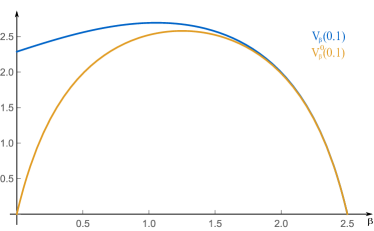
(a) $|x|=0.1$

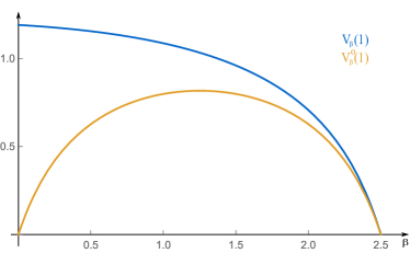
(b) $|x|=1$

Figure 1. Comparison of $V_{\beta}(x)$ and $V_{\beta}^{0}(x)=\kappa_{\beta}|x|^{-\alpha}$ for $d=3$, $\alpha=1/2$.

We will later on need the following technical result that provides the upper bound of the difference $V_{\beta}(x)-\kappa_{\beta}|x|^{-\alpha}$, which is uniform in the parameter $\beta$.

Lemma 2.11.

Let $0<\beta_{0}<\alpha\land(d-\alpha)$. There exists $c>0$ such that for all $\beta\in[\beta_{0},d-\alpha)$ and $0<|x|\leq 1$,

$$V_{\beta}(x)-\kappa_{\beta}|x|^{-\alpha}\leq c|x|^{\beta_{0}-\alpha}\,.$$

Proof.

By Lemma 2.9, (2.11) and (A.5),

$$V_{\beta}(x)-\kappa_{\beta}|x|^{-\alpha}\leq\kappa_{\frac{d-\alpha}{2}}|x|^{-\alpha}\frac{V_{\beta_{0}}(1)}{\kappa_{\beta_{0}}}\int_{0}^{|x|}\frac{K_{\frac{\beta_{0}}{2}-1}(s)}{K_{\frac{\beta_{0}}{2}}(s)}\,{\rm d}{s}\,.$$

Then we use the third limit from the proof of Lemma 2.10. ∎

3. Heat kernel of $-(-\Delta)^{\alpha/2}+V_{\delta}$

In this section we assume that $\alpha\in(0,2\land d)$. Before treating the transition density for the operator (1.1), we first analyse the one corresponding to $-(-\Delta)^{\alpha/2}+V_{\delta}$. Namely, we consider the heat kernel $p^{0}$ of $-(-\Delta)^{\alpha/2}$, see (2.8) for the definition, and we concentrate on $\tilde{p}^{\,0}_{V_{\delta}}$ that is the Schrödinger perturbation of $p^{0}$ by $V_{\delta}$. As an auxiliary function we use $\tilde{p}^{\,0}_{V^{0}_{\delta}}$ that is the Schrödinger perturbation of $p^{0}$ by $V^{0}_{\delta}(z)=\kappa_{\delta}|z|^{-\alpha}$, which was thoroughly investigated in [12]. By Corollary 2.7 we have for $\delta\in(0,d-\alpha)$ that

$$0\leq V^{0}_{\delta}\leq V_{\delta}\qquad\mbox{and}\qquad\tilde{p}^{\,0}_{V_{\delta}^{0}}\leq\tilde{p}^{\,0}_{V_{\delta}}\,.$$

In Proposition 3.4 below we show that the converse of the latter inequality holds up to multiplicative constant. We first prove two auxiliary results.

Lemma 3.1.

Let $\beta\in(0,d)$ and $\gamma\in[\beta-\alpha,\infty)$. There is a constant $c>0$ such that for all $t>0$, $x\in\mathbb{R}^{d}$,

$$\int_{0}^{t}\int_{\mathbb{R}^{d}}s^{\gamma/\alpha}p^{0}(s,x,z)|z|^{-\beta}\,{\rm d}{z}{\rm d}{s}\leq c\begin{cases}t^{(\gamma+\alpha)/\alpha}\left(t^{-\beta/\alpha}\land|x|^{-\beta}\right)\quad&{\rm for}\,\,\gamma>\beta-\alpha\,,\\ \\ \log(1+t^{\beta/\alpha}|x|^{-\beta})&{\rm for}\,\,\gamma=\beta-\alpha\,.\end{cases}$$

Proof.

By [12, Lemma 2.3],

$$\int_{\mathbb{R}^{d}}p^{0}(s,x,z)|z|^{-\beta}{\rm d}{z}\leq c(s^{-\beta/\alpha}\land|x|^{-\beta})\,.$$

Hence, for $|x|^{\alpha}\geq t$,

$$\int_{0}^{t}\int_{\mathbb{R}^{d}}s^{\gamma/\alpha}p^{0}(s,x,z)|z|^{-\beta}{\rm d}{z}{\rm d}{s} \leq c|x|^{-\beta}\int_{0}^{t}s^{\gamma/\alpha}{\rm d}{s}=\frac{c\alpha}{\gamma+\alpha}t^{(\gamma+\alpha)/\alpha}|x|^{-\beta}\,.$$

Let $|x|^{\alpha}<t$. For $\gamma>\beta-\alpha$,

$$\int_{0}^{t}\int_{\mathbb{R}^{d}}s^{\gamma/\alpha}p^{0}(s,x,z)|z|^{-\beta}{\rm d}{z}{\rm d}{s} \leq c|x|^{-\beta}\int_{0}^{|x|^{\alpha}}s^{\gamma/\alpha}{\rm d}{s}+c\int_{|x|^{\alpha}}^{t}s^{(\gamma-\beta)/\alpha}{\rm d}{s}\leq ct^{(\gamma+\alpha-\beta)/\alpha}\,.$$

The same steps lead to the second estimate for $\gamma=\beta-\alpha$. ∎

Lemma 3.2.

Let $\delta\in(0,\frac{d-\alpha}{2}]$ and $0<\delta<\alpha$. There is a constant $c>0$ such that for all $t>0$, $x,y\in\mathbb{R}^{d}_{0}$,

$$\int_{0}^{t}\int_{\mathbb{R}^{d}}\tilde{p}^{\,0}_{V^{0}_{\delta}}(s,x,z)|z|^{\delta-\alpha}\,\tilde{p}^{\,0}_{V^{0}_{\delta}}(t-s,z,y)\,{\rm d}{z}{\rm d}{s}\leq ct^{\delta/\alpha}\tilde{p}^{\,0}_{V_{\delta}^{0}}(t,x,y)\,.$$

Proof.

Recall from [12, Theorem 1.1 and (2.4)] that

$$\tilde{p}^{\,0}_{V^{0}_{\delta}}(t,x,y)\approx p^{0}(t,x,z)H^{0}(t,x)H^{0}(t,y)\,,$$ (3.1)

where $H^{0}(t,x)=1+t^{\delta/\alpha}|x|^{-\delta}$ as introduced in Section 1. Note that for $0<s<t$ we have $H^{0}(t-s,y)\leq H^{0}(t,y)$ and

$$H^{0}(s,x)H^{0}(s,z)H^{0}(t-s,z) \leq H^{0}(s,z)H^{0}(s,x)H^{0}(t,z)$$

$$\leq H^{0}(s,z)\left(H^{0}(t,x)H^{0}(s,z)+\frac{t^{\delta/\alpha}}{|z|^{\delta}}\right)$$

$$=H^{0}(t,x)\left(1+\frac{2s^{\delta/\alpha}}{|z|^{\delta}}+\frac{s^{2\delta/\alpha}}{|z|^{2\delta}}\right)+t^{\delta/\alpha}\left(\frac{1}{|z|^{\delta}}+\frac{s^{\delta/\alpha}}{|z|^{2\delta}}\right).$$

By Lemma 3.1 we get for $k\in\{0,1,2\}$,

$$\int_{0}^{t}\int_{\mathbb{R}^{d}}s^{k\delta/\alpha}p^{0}(s,x,z)|z|^{-k\delta}|z|^{\delta-\alpha}\,{\rm d}{z}{\rm d}{s}\leq ct^{\delta/\alpha}\,,$$

and for $k\in\{0,1\}$,

$$\int_{0}^{t}\int_{\mathbb{R}^{d}}s^{k\delta/\alpha}p^{0}(s,x,z)|z|^{-(k+1)\delta}|z|^{\delta-\alpha}\,{\rm d}{z}{\rm d}{s}\leq c\log\left(1+\left(t|x|^{-\alpha}\right)^{k\delta/\alpha+1}\right)\leq cH^{0}(t,x)\,.$$

Thus

$$\int_{0}^{t}\int_{\mathbb{R}^{d}}p^{0}(s,x,z)H^{0}(s,x)H^{0}(s,z)H^{0}(t-s,y)H^{0}(t-s,z)|z|^{\delta-\alpha}\,{\rm d}{z}{\rm d}{s}\leq ct^{\delta/\alpha}H^{0}(t,x)H^{0}(t,y)\,.$$

Similarly,

$$\int_{0}^{t}\int_{\mathbb{R}^{d}}p^{0}(t-s,z,y)H^{0}(s,x)H^{0}(s,z)H^{0}(t-s,y)H^{0}(t-s,z)|z|^{\delta-\alpha}{\rm d}{z}{\rm d}{s}\leq ct^{\delta/\alpha}H^{0}(t,x)H^{0}(t,y)\,.$$

Finally, the result follows from the latter two inequalities combined with

$$\tilde{p}^{\,0}_{V^{0}_{\delta}}(s,x,z)\tilde{p}^{\,0}_{V^{0}_{\delta}}(t-s,z,y)$$

$$\leq cp^{0}(t,x,y)\Big{(}p^{0}(s,x,z)+p^{0}(t-s,z,y)\Big{)}H^{0}(s,x)H^{0}(s,z)H^{0}(t-s,y)H^{0}(t-s,z)\,,$$

which holds by (3.1) and 3G-inequality for $p^{0}(t,x,y)$, see [14, Theorem 4]. ∎

We show that $V_{\delta}-V^{0}_{\delta}$ can be conveniently used to perturb $\tilde{p}^{\,0}_{V_{\delta}^{0}}$.

Corollary 3.3.

Let $\delta\in(0,\frac{d-\alpha}{2}]$. For every $T>0$ there is a constant $c>0$ such that for all $t\in(0,T]$ and $x,y\in\mathbb{R}^{d}_{0}$,

$$\int_{0}^{t}\int_{\mathbb{R}^{d}}\tilde{p}^{\,0}_{V^{0}_{\delta}}(s,x,z)\Big{(}V_{\delta}(z)-V^{0}_{\delta}(z)\Big{)}\tilde{p}^{\,0}_{V^{0}_{\delta}}(t-s,z,y)\,{\rm d}{z}{\rm d}{s}\leq c\max\{t,t^{\delta/\alpha}\}\,\tilde{p}^{\,0}_{V_{\delta}^{0}}(t,x,y)\,.$$

Proof.

Let $q(z):=V_{\delta}(z)-V^{0}_{\delta}(z)=V_{\delta}(z)-\kappa_{\delta}|z|^{-\alpha}\geq 0$, see Corollary 2.7. If $\delta\geq\alpha$ the inequality is trivial, because due to Lemmas 2.8 and 2.10 the function $q$ is bounded, and $\tilde{p}^{\,0}_{V_{\delta}^{0}}$ satisfies Chapman-Kolmogorov equation (2.2). If $0<\delta<\alpha$, then $q$ is bounded for $|z|\geq 1/2$, while for $|z|\leq 1/2$ we can use Lemmas 2.10 and 3.2 to obtain the desired inequality. ∎

Proposition 3.4.

Let $\delta\in(0,d-\alpha)$. For every $T>0$ there is a constant $c>0$ such that for all $t\in(0,T]$ and $x,y\in\mathbb{R}^{d}_{0}$,

$$\tilde{p}^{\,0}_{V_{\delta}}(t,x,y)\leq c\,\tilde{p}^{\,0}_{V_{\delta}^{0}}(t,x,y)\,.$$

Proof.

According to (2.3) we treat $\tilde{p}^{\,0}_{V_{\delta}}$ as the perturbation of $\tilde{p}^{\,0}_{V^{0}_{\delta}}$ by $q_{\delta}(z):=V_{\delta}(z)-V^{0}_{\delta}(z)=V_{\delta}(z)-\kappa_{\delta}|z|^{-\alpha}\geq 0$, see Corollary 2.7. If $\delta\in(0,\frac{d-\alpha}{2}]$ the result follows from [13, Theorem 2] since $q$ is relatively Kato for $\tilde{p}^{\,0}_{V_{\delta}^{0}}$ by Corollary 3.3. If $\delta\in[\frac{d-\alpha}{2},d-\alpha)$ the same argument applies, because $0\leq q_{\delta}\leq q_{\delta^{\prime}}$ with $\delta^{\prime}=d-\alpha-\delta\in(0,\frac{d-\alpha}{2}]$, see Remark 2.2. ∎

We will use the following observation several times throughout the paper.

Remark 3.1.

Let $\delta\in(0,d-\alpha)$. Recall that $\tilde{p}:=\tilde{p}_{V_{\delta}}$ is the Schrödinger perturbation of $p:=p^{1}$ by $V_{\delta}:=V^{1}_{\delta}$. Directly from (2.8) we have $p\leq p^{0}$, and by Proposition 3.4,

$$\tilde{p}\leq\tilde{p}^{\,0}_{V_{\delta}}\leq c\,\tilde{p}^{\,0}_{V_{\delta}^{0}}$$

holds on $(0,T]\times\mathbb{R}^{d}_{0}\times\mathbb{R}^{d}_{0}$, whenever $\delta\in(0,d-\alpha)$ and $T>0$ are fixed.

We are ready to show Proposition 1.1. The essence of the proof is to take a similar equality for the original transition density $p$ and the operator $\partial_{u}-(-\Delta_{z}+1)^{\alpha/2}$, and to use the algebraic structure of the perturbed transition density $\tilde{p}$. That idea goes back to [13, (39)], [16, Lemma 4] and [10, Lemma 2.1]. In doing so one should ensure that certain integrals converge absolutely. This can be guaranteed using Proposition 3.4 and [12, Proposition 3.2].

Proof of Proposition 1.1.

Recall that $\tilde{p}:=\tilde{p}_{V_{\delta}}$ that is the perturbation of $p:=p^{1}$ by $V_{\delta}:=V^{1}_{\delta}$. For $s\in\mathbb{R}$ and $x\in\mathbb{R}^{d}_{0}$ we define

$$Pf(s,x) =\int_{s}^{\infty}\int_{\mathbb{R}^{d}}p(u-s,x,z)f(u,z)\,{\rm d}{z}{\rm d}{u}\,,$$

$$\tilde{P}f(s,x) =\int_{s}^{\infty}\int_{\mathbb{R}^{d}}\tilde{p}(u-s,x,z)f(u,z)\,{\rm d}{z}{\rm d}{u}\,,$$

$$V_{\delta}f(s,x) =V_{\delta}(x)f(s,x)\,.$$

for a jointly measurable function $f$ such that the integrals converge absolutely. Let $\psi(u,z)=\left(\partial_{u}-(-\Delta_{z}+1)^{\alpha/2}\right)\phi(u,z)$. It is well known that for all $s\in\mathbb{R}$, $x\in\mathbb{R}^{d}$ and $\phi\in C_{c}^{\infty}(\mathbb{R}\times\mathbb{R}^{d})$ we have (see [10, Theorem 4.1 and (1.16)])

$$\int_{s}^{\infty}\int_{\mathbb{R}^{d}}p(u-s,x,z)\left[\partial_{u}-(-\Delta_{z}+1)^{\alpha/2}\right]\phi(u,z)\,{\rm d}{z}{\rm d}{u}=-\phi(s,x)\,.$$

Hence, $P\psi=-\phi$. Then,

$$\tilde{P}(\psi+V_{\delta}\phi)=(P+\tilde{P}V_{\delta}P)\psi+\tilde{P}V_{\delta}\phi=-\phi+\tilde{P}V_{\delta}P\psi+\tilde{P}V_{\delta}(-P\psi)=-\phi\,,$$

which is the desired equality, but we need to make sure that the integrals converge absolutely. We consider

$$\tilde{P}^{0}f(s,x)=\int_{s}^{\infty}\int_{\mathbb{R}^{d}}\tilde{p}^{\,0}_{V_{\delta}^{0}}(u-s,x,z)f(u,z)\,{\rm d}{z}{\rm d}{s}\,.$$

Note that the function $\psi$ is bounded [61, p. 211] and zero if $|u|$ is large. By Remark 3.1, for every $s\in\mathbb{R}$ and $x\in\mathbb{R}^{d}_{0}$ there is $c$ such that

$$\tilde{P}|\psi|(s,x)\leq c\tilde{P}^{0}|\psi|(s,x)<\infty\,.$$

The finiteness follows from [12, Proposition 3.2] and because $\tilde{P}^{0}$ is the same for $\delta$ and $\delta^{\prime}=d-\alpha-\delta$, see Remark 2.2. This implies that $P|\psi|$, $\tilde{P}|\psi|$, $\tilde{P}V_{\delta}P|\psi|$ and $\tilde{P}V_{\delta}|\phi|$ are finite. Indeed, by (2.1) we have

$$P|\psi|+\tilde{P}V_{\delta}P|\psi|=\tilde{P}|\psi|<\infty\qquad\mbox{and}\qquad\tilde{P}V_{\delta}|\phi|\leq\tilde{P}V_{\delta}P|\psi|<\infty\,.$$

∎

Proposition 3.5.

Let $\delta\in(0,d-\alpha)$. If $m\downarrow 0$, then for all $t>0$, $x,y\in\mathbb{R}^{d}_{0}$,

$$p^{m}(t,x,y)\uparrow p^{0}(t,x,y)\,,\qquad\quad V_{\delta}^{m}(x)\downarrow V_{\delta}^{0}(x)\,,\qquad\quad\tilde{p}^{\,m}(t,x,y)\to\tilde{p}^{\,0}(t,x,y)\,.$$

Proof.

The convergence and monotonicity of $p^{m}$ follows from (2.8). The convergence of $V_{\delta}^{m}$ stems from Lemmas 2.6 and 2.2, and the monotonicity from (2.11). To prove the third convergence we use the dominated convergence theorem. To justify its use we note that $p^{m}\leq p^{0}$ and $V_{\delta}^{m}\leq V_{\delta}^{1}$ if $m\in(0,1]$, and we let $\tilde{p}^{\,0}_{V_{\delta}}$ (the Schrödinger perturbation of $p^{0}$ by $V_{\delta}=V_{\delta}^{1}$) to be the majorant, see also Proposition 3.4 for summability or integrability. ∎

4. Heat kernel of $-(-\Delta+1)^{\alpha/2}+V_{\delta}$

Under the constraint in the whole section that $\alpha\in(0,2\land d)$ and $\delta\in(0,\frac{d-\alpha}{2}]$ we finally consider the transition density $\tilde{p}$ for the operator (1.1). As specified after Theorem 4.12 and in the comment preceding Lemma 2.4, we investigate $\tilde{p}:=\tilde{p}_{V_{\delta}}$ that is the Schrödinger perturbation of $p:=p^{1}$ by $V_{\delta}:=V^{1}_{\delta}$.

4.1. Upper bound

We consider the following function

$$H(t,x):=1+\frac{h_{\delta}(x)}{h_{\delta}(t^{1/\alpha})}\,.$$

Note that for every $T>0$ we have on $(0,T]\times\mathbb{R}^{d}_{0}$ (see Lemma 2.3 and (A.1)),

$$H(t,x)\approx H^{0}(t,x)\,.$$ (4.1)

Proposition 4.1.

For every $T,R>0$ there exists a constant $c$ such that for all $t\in(0,T]$ and $x,y\in\mathbb{R}^{d}_{0}$ satisfying $|x-y|\leq R$,

$$\tilde{p}(t,x,y)\leq cp(t,x,y)H(t,x)H(t,y)\,.$$

Proof.

By Remark 3.1 and (3.1) we have $\tilde{p}(t,x,y)\leq cp^{0}(t,x,y)H^{0}(t,x)H^{0}(t,y)$. Now, due to (4.1) it suffices to observe that $p^{0}(t,x,y)\leq c(t^{-d/\alpha}\land\frac{t}{|x-y|^{d+\alpha}})\leq cp(t,x,y)\,,$ whenever $t\in(0,T]$ and $|x-y|\leq R$, see e.g. [12, (2.4)] and (A.9). ∎

Recall that $V_{\delta}$ is radial decreasing (see Lemma 2.8) thus we can define the inverse of its radial profile, which we denote by $V_{\delta}^{-1}$.

Lemma 4.2.

For all $t>0$ and $x,y\in\mathbb{R}^{d}_{0}$,

$$\tilde{p}(t,x,y)\leq 2p(t,x,y)+2\int_{0}^{t}\int_{|z|\leq V_{\delta}^{-1}(\frac{1}{2t})}\tilde{p}(t-s,x,z)V_{\delta}(z)p(s,z,y)\,{\rm d}{z}{\rm d}{s}\,.$$ (4.2)

Proof.

By Duhamel’s formula (2.1), the monotonicity of $V_{\delta}$ and Chapman-Kolmogorov equation (2.2), for any $R>0$ we have

$$\tilde{p}(t,x,y) =p(t,x,y)+\int_{0}^{t}\int_{|z|\leq R}\tilde{p}(t-s,x,z)V_{\delta}(z)p(s,z,y)\,{\rm d}{z}{\rm d}{s}$$

$$\qquad\qquad\qquad+\int_{0}^{t}\int_{|z|>R}\tilde{p}(t-s,x,z)V_{\delta}(z)p(s,z,y)\,{\rm d}{z}{\rm d}{s}$$

$$\leq p(t,x,y)+\int_{0}^{t}\int_{|z|\leq R}\tilde{p}(t-s,x,z)V_{\delta}(z)p(s,z,y)\,{\rm d}{z}{\rm d}{s}+tV_{\delta}(R)\tilde{p}(t,x,y)\,.$$

It suffices to take $V_{\delta}(R)=1/(2t)$. ∎

Proposition 4.3.

Let $T>0$. There exists a constant $c$ such that for all $t\in(0,T]$, $x\in\mathbb{R}^{d}_{0}$,

$$\int_{\mathbb{R}^{d}}\tilde{p}(t,x,y)\,{\rm d}{y}\leq cH(t,x)\,.$$ (4.3)

Proof.

Integrating (4.2) we get

$$\int_{\mathbb{R}^{d}}\tilde{p}(t,x,y)\,{\rm d}{y}\leq 2+2\int_{0}^{t}\int_{|z|\leq V_{\delta}^{-1}(\frac{1}{2t})}\tilde{p}(t-s,x,z)V_{\delta}(z)\,{\rm d}{z}{\rm d}{s}\,.$$

Note that by Lemma 2.6 there is $c_{1}$ such that $V_{\delta}^{-1}(\frac{1}{2t})\leq c_{1}t^{1/\alpha}$ for all $t\in(0,T]$. Thus, by (A.9) there is $c_{2}>0$ such that for all $0<s<t\leq T$ and $|z|\leq V_{\delta}^{-1}(\frac{1}{2t})$,

$$c_{2}\leq\int_{|y|\leq 2c_{1}t^{1/\alpha}}p(s,z,y)\,{\rm d}{y}\,.$$

Then, by (2.1) in the second inequality,

$$\int_{\mathbb{R}^{d}}\tilde{p}(t,x,y)\,{\rm d}{y} \leq 2+\frac{2}{c_{2}}\int_{|y|\leq 2c_{1}t^{1/\alpha}}\left(\int_{0}^{t}\int_{|z|\leq V_{\delta}^{-1}(\frac{1}{2t})}\tilde{p}(t-s,x,z)V_{\delta}(z)p(s,z,y)\,{\rm d}{z}{\rm d}{s}\right){\rm d}{y}$$

$$\leq 2+\frac{2}{c_{2}}\int_{|y|\leq 2c_{1}t^{1/\alpha}}\tilde{p}(t,x,y)\,{\rm d}{y}\,.$$

Now, by the monotonicity of $h_{\delta}$ and Corollary 2.5 we get

$$\int_{|y|\leq 2c_{1}t^{1/\alpha}}\tilde{p}(t,x,y)\,{\rm d}{y}\leq\frac{1}{h_{\delta}(2c_{1}t^{1/\alpha})}\int_{|y|\leq 2c_{1}t^{1/\alpha}}\tilde{p}(t,x,y)h_{\delta}(y)\,{\rm d}{y}\leq\frac{h_{\delta}(x)}{h_{\delta}(2c_{1}t^{1/\alpha})}\,.$$

Finally, note that $h_{\delta}(2c_{1}t^{1/\alpha})\approx h_{\delta}(t^{1/\alpha})$ for $t\in(0,T]$. ∎

In what follows, for $T>0$ we set

$$R_{0}:=\max\{1,V_{\delta}^{-1}(1/(2T))\}\,.$$

We shall also use $\nu(x)$ defined in Corollary 1.3.

Lemma 4.4.

Let $T>0$. There exists a constant $c$ such that for all $t\in(0,T]$, $R\in[R_{0},2R_{0}]$ and $0<|x|\leq R$, $|y|\geq R+1$,

$$\tilde{p}(t,x,y)\leq ct\nu(x-y)H(t,x)\,.$$

Proof.

Since $|x|\leq 2R_{0}$, $|y|\geq R_{0}+1$, using (A.8) and (A.6) we get $p(s,z,y)\leq cs\nu(x-y)$ for all $s\in(0,T]$ and $|z|\leq R_{0}$. Thus, by (4.2) we have

$$\tilde{p}(t,x,y) \leq 2p(t,x,y)+2\int_{0}^{t}\int_{|z|\leq R_{0}}\tilde{p}(t-s,x,z)V_{\delta}(z)p(s,z,y)\,{\rm d}{z}{\rm d}{s}$$

$$\leq ct\nu(x-y)+ct\nu(x-y)\int_{0}^{t}\int_{|z|\leq R_{0}}\tilde{p}(t-s,x,z)V_{\delta}(z)\,{\rm d}{z}{\rm d}{s}\,.$$

Furthermore, by (2.1) and (4.3) we have

$$\int_{0}^{t}\int_{\mathbb{R}^{d}}\tilde{p}(t-s,x,z)V_{\delta}(z)\,{\rm d}{z}{\rm d}{s}\leq\int_{\mathbb{R}^{d}}\tilde{p}(t,x,y)\,{\rm d}{y}\leq cH(t,x)\,.$$

∎

Proposition 4.5.

Let $T>0$. There exists a constant $c$ such that for all $t\in(0,T]$ and $|x|\vee|y|\geq 3R_{0}$,

$$\tilde{p}(t,x,y)\leq ct\nu(x-y)H(t,x)H(t,y)\,.$$

Proof.

By the symmetry of $\tilde{p}$ we may and do assume that $|y|\geq 3R_{0}$. The case of $|x|\leq 2R_{0}$ is covered by Lemma 4.4 with $R=2R_{0}$. From now on we consider $|x|\geq 2R_{0}$. Using the symmetry of $\tilde{p}$ again, we get by (4.2) that

$$\tilde{p}(t,x,y) \leq 2p(t,y,x)+2\int_{0}^{t}\int_{|z|\leq R_{0}}\tilde{p}(t-s,z,y)V_{\delta}(z)p(s,z,x)\,{\rm d}{z}{\rm d}{s}\,.$$

Furthermore, by Lemma 4.4 with $R=R_{0}$, we have by the monotonicity of $h_{\delta}$ that for $0<s<t\leq T$ and $|z|\leq R_{0}$,

$$\tilde{p}(t-s,z,y)\leq cT\nu(z-y)H(T,z)\,.$$

Thus, by (A.8) and (A.7) we have

$$\tilde{p}(t,x,y) \leq ct\nu(x-y)+cT^{2}\int_{0}^{t}\int_{|z|\leq R_{0}}\nu(z-y)H(T,z)V_{\delta}(z)\nu(x-z)\,{\rm d}{z}{\rm d}{s}$$

$$\leq ct\nu(x-y)+cT^{2}\nu(x-y)\int_{0}^{t}\int_{|z|\leq R_{0}}H(T,z)V_{\delta}(z)\,{\rm d}{z}{\rm d}{s}$$

$$=ct\nu(x-y)+ct\nu(x-y)\,T^{2}\int_{|z|\leq R_{0}}H(T,z)V_{\delta}(z)\,{\rm d}{z}\,.$$

Finally, notice that $\int_{|z|\leq R_{0}}H(T,z)V_{\delta}(z)\,{\rm d}{z}<\infty$ since $\alpha<d$, and $H(t,x)H(t,y)\geq 1$. ∎

Theorem 4.6.

Let $T>0$. There exists a constant $c$ such that for all $t\in(0,T]$ and $x,y\in\mathbb{R}^{d}_{0}$,

$$\tilde{p}(t,x,y)\leq cp(t,x,y)H(t,x)H(t,y)\,.$$

Proof.

If $|x-y|\leq 6R_{0}$, the inequality follows from Proposition 4.1. If $|x-y|\geq 6R_{0}$, then $|x|\vee|y|\geq 3R_{0}$ and the inequality holds by Proposition 4.5 and (A.10). ∎

4.2. Invariance of $h_{\delta}$

We show that in fact there is equality in Corollary 2.5 if $\delta\in(0,\frac{d-\alpha}{2}]$. Recall that the functions $h_{\beta}:=h^{1}_{\beta}$ and $\bar{h}_{\beta}:=\bar{h}^{1}_{\beta}$ are defined in Subsection 2.3.

Lemma 4.7.

For all $\beta\in(0,d-\alpha)$ and $t>0$, $x\in\mathbb{R}^{d}_{0}$,

$$\int_{\mathbb{R}^{d}}p(t,x,y)h_{\beta}(y)\,{\rm d}{y}+\int_{0}^{t}\int_{\mathbb{R}^{d}}p(s,x,y)\bar{h}_{\beta}(y)\,{\rm d}{y}{\rm d}{s}=h_{\beta}(x)\,.$$

Proof.

Let $f(t)=t^{\frac{d-\alpha-\beta}{\alpha}}$. Then

$$\int_{0}^{t}\int_{\mathbb{R}^{d}}p(s,x,y)\bar{h}_{\beta}(y)\,{\rm d}{y}{\rm d}{s} =\int_{0}^{t}\int_{0}^{\infty}p(s+r,x,0)f^{\prime}(r)\,{\rm d}{r}{\rm d}{s}$$

$$=-\int_{0}^{t}\int_{0}^{\infty}\partial_{s}\,p(s+r,x,0)f(r)\,{\rm d}{r}{\rm d}{s}$$

$$=\int_{0}^{\infty}[p(r,x,0)-p(t+r,x,0)]f(r)\,{\rm d}{r}$$

$$=h_{\beta}(x)-\int_{\mathbb{R}^{d}}p(t,x,y)h_{\beta}(y)\,{\rm d}{y}\,.$$

In the second equality above we used integration by parts and that $p(s+r,x,0)f(r)\leq p^{0}(s+r,x,0)f(r)$ vanishes at zero and at infinity as a function of $r$. In the third equality we used Fubini’s theorem, which was justified because $\int_{0}^{t}\int_{0}^{\infty}|\frac{\partial}{\partial s}\,p(s+r,x,0)f(r)|\,{\rm d}{r}{\rm d}{s}<\infty$, see Lemma A.3. ∎

Here is how Lemma 4.7 propagates onto $\tilde{p}$.

Proposition 4.8.

For all $\beta\in(0,d-\alpha)$ and $t>0$, $x\in\mathbb{R}^{d}_{0}$,

$$\int_{\mathbb{R}^{d}}\tilde{p}(t,x,y)h_{\beta}(y)\,{\rm d}{y}+\int_{0}^{t}\int_{\mathbb{R}^{d}}\tilde{p}(s,x,y) \bar{h}_{\beta}(y)\,{\rm d}{y}{\rm d}{s}$$

$$=h_{\beta}(x)+\int_{0}^{t}\int_{\mathbb{R}^{d}}\tilde{p}(s,x,y)V_{\delta}(y)h_{\beta}(y)\,{\rm d}{y}{\rm d}{s}\,.$$

Proof.

By Duhamel’s formula (2.1),

$$\int_{\mathbb{R}^{d}}\tilde{p}(t,x,y)h_{\beta}(y)\,{\rm d}{y}$$

$$\qquad=\int_{\mathbb{R}^{d}}p(t,x,y)h_{\beta}(y)\,{\rm d}{y}+\int_{0}^{t}\int_{\mathbb{R}^{d}}\tilde{p}(s,x,z)V_{\delta}(z)\int_{\mathbb{R}^{d}}p(t-s,z,y)h_{\beta}(y)\,{\rm d}{y}\,{\rm d}{z}{\rm d}{s}\,,$$

and

$$\int_{0}^{t}\int_{\mathbb{R}^{d}}\tilde{p}(s,x,y)\bar{h}_{\beta}(y)\,{\rm d}{y}{\rm d}{s}$$

$$\qquad=\int_{0}^{t}\int_{\mathbb{R}^{d}}p(s,x,y)\bar{h}_{\beta}(y)\,{\rm d}{y}{\rm d}{s}+\int_{0}^{t}\int_{\mathbb{R}^{d}}\int_{0}^{s}\int_{\mathbb{R}^{d}}\tilde{p}(u,x,z)V_{\delta}(z)p(s-u,z,y)\,{\rm d}{z}{\rm d}{u}\,\bar{h}_{\beta}(y)\,{\rm d}{y}{\rm d}{s}$$

$$\qquad=\int_{0}^{t}\int_{\mathbb{R}^{d}}p(s,x,y)\bar{h}_{\beta}(y)\,{\rm d}{y}{\rm d}{s}+\int_{0}^{t}\int_{\mathbb{R}^{d}}\tilde{p}(u,x,z)V_{\delta}(z)\int_{0}^{t-u}\int_{\mathbb{R}^{d}}p(r,z,y)\bar{h}_{\beta}(y)\,{\rm d}{y}{\rm d}{r}\,{\rm d}{z}{\rm d}{u}$$

$$\qquad=\int_{0}^{t}\int_{\mathbb{R}^{d}}p(s,x,y)\bar{h}_{\beta}(y)\,{\rm d}{y}{\rm d}{s}+\int_{0}^{t}\int_{\mathbb{R}^{d}}\tilde{p}(s,x,z)V_{\delta}(z)\int_{0}^{t-s}\int_{\mathbb{R}^{d}}p(r,z,y)\bar{h}_{\beta}(y)\,{\rm d}{y}{\rm d}{r}\,{\rm d}{z}{\rm d}{s}\,.$$

It suffices to add the above expressions and apply Lemma 4.7. ∎

Recall that we assume $\delta\in(0,\frac{d-\alpha}{2}]$. Given the equality in Proposition 4.8, we would like to put $\beta=\delta$ and to cancel the double integrals, because $\bar{h}_{\delta}(x)=V_{\delta}(x)h_{\delta}(x)$, $x\in\mathbb{R}^{d}_{0}$. That would require the finiteness of these integrals. We also note that the case $\delta=\frac{d-\alpha}{2}$ is more challenging than that of $\delta<\frac{d-\alpha}{2}$. We prove both cases at once by a limiting procedure.

Theorem 4.9.

For all $t>0$ and $x\in\mathbb{R}^{d}_{0}$,

$$\int_{\mathbb{R}^{d}}\tilde{p}(t,x,y)h_{\delta}(y)\,{\rm d}{y}=h_{\delta}(x)\,.$$

Proof.

By the definition of $h_{\beta}^{m}$ in Subsection 2.3 we have

$$h_{\beta}(y)\leq h_{\beta}^{0}(y)=\frac{2^{\beta}\Gamma\left(\frac{d-\beta}{\alpha}\right)\Gamma\left(\frac{\beta}{2}\right)}{(4\pi)^{d/2}\Gamma\left(\frac{d-\beta}{2}\right)}|y|^{-\beta}\,.$$

Thus, by Remark 3.1 and [12, (3.3)], for $0<\beta<\delta$ the integrals on the left hand side of the equality in Proposition 4.8 are finite, hence the one on the right hand side is also finite, and we can rewrite the equality as

$$\int_{\mathbb{R}^{d}}\tilde{p}(t,x,y)h_{\beta}(y)\,{\rm d}{y}=h_{\beta}(x)+\int_{0}^{t}\int_{\mathbb{R}^{d}}\tilde{p}(s,x,y)\Big{(}V_{\delta}(y)-V_{\beta}(y)\Big{)}h_{\beta}(y)\,{\rm d}{y}{\rm d}{s}\,.$$

Fix $0<\beta_{0}<\alpha\land\delta$. For $\beta\in[\beta_{0},\delta]$ we have $h_{\beta}(x)\leq\sup_{\beta\in[\beta_{0},\delta]}h_{\beta}^{0}(1)(|x|^{-\delta}+1)$, therefore by Remark 3.1 and [12, (3.2) and Proposition 3.2] we can apply the dominated convergence theorem to the integral on the left hand side,

$$\lim_{\beta\uparrow\delta}\int_{\mathbb{R}^{d}}\tilde{p}(t,x,y)h_{\beta}(y)\,{\rm d}{y}=\int_{\mathbb{R}^{d}}\tilde{p}(t,x,y)h_{\delta}(y)\,{\rm d}{y}\,.$$

Now, we split the integral on the right hand side,

$$\int_{0}^{t}\int_{\mathbb{R}^{d}}\tilde{p}(s,x,y)\Big{(}V_{\delta}(y)-V_{\beta}(y)\Big{)}h_{\beta}(y)\,{\rm d}{y}{\rm d}{s}=I_{1}+I_{2}+I_{3}+I_{4}\,,$$

where

$$I_{1} =\int_{0}^{t}\int_{|y|\geq r_{0}}\tilde{p}(s,x,y)\Big{(}V_{\delta}(y)-V_{\beta}(y)\Big{)}h_{\beta}(y)\,{\rm d}{y}{\rm d}{s}\,,$$

$$I_{2} =(\kappa_{\delta}-\kappa_{\beta})\int_{0}^{t}\int_{|y|<r_{0}}\tilde{p}(s,x,y)|y|^{-\alpha}h_{\beta}(y)\,{\rm d}{y}{\rm d}{s}\,,$$

$$I_{3} =\int_{0}^{t}\int_{|y|<r_{0}}\tilde{p}(s,x,y)\Big{(}V_{\delta}(y)-\kappa_{\delta}|y|^{-\alpha}\Big{)}h_{\beta}(y)\,{\rm d}{y}{\rm d}{s}\,,$$

$$I_{4} =-\int_{0}^{t}\int_{|y|<r_{0}}\tilde{p}(s,x,y)\Big{(}V_{\beta}(y)-\kappa_{\beta}|y|^{-\alpha}\Big{)}h_{\beta}(y)\,{\rm d}{y}{\rm d}{s}\,,$$

and the value of $r_{0}\in(0,1]$ will be specified later. Clearly, $I_{2}\geq 0$ and $I_{3}\geq 0$. All the following inequalities will be uniform in $\beta\in[\beta_{0},\delta]$. By Lemma 2.11 for all $0<|y|\leq 1$,

$$|V_{\beta}(y)-\kappa_{\beta}|y|^{-\alpha}|h_{\beta}(y)\leq c|y|^{\beta_{0}-\alpha}\sup_{\beta\in[\beta_{0},\delta]}h_{\beta}(1)|y|^{-\delta}=c^{\prime}|y|^{\beta_{0}-\delta-\alpha}\,.$$

Fix $\varepsilon>0$. Since by [12, (3.3)] with $\beta=\delta-\beta_{0}$ the latter expression is integrable against $\tilde{p}^{\,0}_{V_{\delta}^{0}}(s,x,y)\,{\rm d}{y}{\rm d}{s}$ on $(0,t]\times\mathbb{R}^{d}$, by Remark 3.1 there is $r_{0}\in(0,1]$ such that $-I_{4}\leq\varepsilon$. Now, for that choice of $r_{0}\in(0,1]$ and all $|y|\geq r_{0}$,

$$|V_{\delta}(y)-V_{\beta}(y)|h_{\beta}(y)\leq\sup_{\beta\in[\beta_{0},\delta]}\Big{(}V_{\delta}(r_{0})+V_{\beta}(r_{0})\Big{)}h_{\beta}(r_{0})<\infty\,.$$

Combined with (4.3) it justifies the usage of the dominated convergence theorem, and we get $\lim_{\beta\uparrow\delta}I_{1}=0$. Finally, we have

$$\int_{\mathbb{R}^{d}}\tilde{p}(t,x,y)h_{\delta}(y)\,{\rm d}{y}\geq h_{\delta}(x)-\varepsilon\,.$$

Since $\varepsilon$ was arbitrary, and in view of Corollary 2.5, we obtain the desired equality. ∎

4.3. Lower bound

We adapt methods developed in [12, Section 4.2]. Let

$$\rho(t,x,y):=\frac{\tilde{p}(t,x,y)}{H(t,x)H(t,y)}\qquad\mbox{and}\qquad\mu_{t}({\rm d}{y}):=[H(t,y)]^{2}{\rm d}{y}\,.$$

Using Theorem 4.9 we get for all $t>0$ and $x\in\mathbb{R}^{d}_{0}$,

$$\int_{\mathbb{R}^{d}}\rho(t,x,z)\,\mu_{t}({\rm d}{z})\geq e^{-t}\,.$$ (4.4)

By Chapman-Kolmogorov equation (2.2) and (4.1), for all $t\in(0,T]$ and $x,y\in\mathbb{R}^{d}_{0}$,

$$\rho(2t,x,y) \geq c\int_{\mathbb{R}^{d}}\rho(t,x,z)\rho(t,z,y)\,\mu_{t}({\rm d}{z})\,.$$ (4.5)

Lemma 4.10.

Let $T>0$. There are $r\in(0,1)$, $R\geq 2$ such that for all $t\in(0,T]$ and $0<|x|\leq(4t)^{1/\alpha}$,

$$\int_{r\leq\frac{|z|}{t^{1/\alpha}}\leq R}\rho(t,x,z)\,\mu_{t}({\rm d}{z})\geq\frac{e^{-T}}{2}\,.$$

Proof.

By Theorem 4.6 we have $\rho(t,x,z)\leq cp(t,x,z)\leq cp^{0}(t,x,z)$, and $H(t,z)\leq cH^{0}(t,z)$. Using the scaling of $p^{0}$ we get from [12, Section 4.2] that the integral of $c^{3}p^{0}$ over $\{|z|\leq rt^{1/\alpha}\}\cup\{|z|\geq Rt^{1/\alpha}\}$ does not exceed $e^{-T}/2$. Therefore, the result follows from (4.4). ∎

Theorem 4.11.

Let $T>0$. There exists a constant $c$ such that for all $t\in(0,T]$ and $x,y\in\mathbb{R}^{d}_{0}$,

$$\tilde{p}(t,x,y)\geq cp(t,x,y)H(t,x)H(t,y)\,.$$

Proof.

If $|x|,|y|\geq t^{1/\alpha}$ we have $H(t,x)H(t,y)\leq 4$, so

$$\rho(t,x,y)\geq\frac{1}{4}\tilde{p}(t,x,y)\geq\frac{1}{4}p(t,x,y)\,.$$ (4.6)

Now, let $r$ and $R$ be taken from Lemma 4.10, which will be used twice below. We first assume that $0<|x|\leq(4t)^{1/\alpha}$ and $|y|\geq r(2t)^{1/\alpha}$. Then by (4.5), (4.1), (A.11) and (A.8) we get for all $t\in(0,T]$,

$$\rho(2t,x,y) \geq c\int_{r\leq\frac{|z|}{t^{1/\alpha}}\leq R}\rho(t,x,z)\rho(t,z,y)\,\mu_{t}({\rm d}{z})\geq c\int_{r\leq\frac{|z|}{t^{1/\alpha}}\leq R}\rho(t,x,z)\frac{p(t,z,y)}{[H^{0}(1,r)]^{2}}\,\mu_{t}({\rm d}{z})$$

$$\geq\frac{c}{[H^{0}(1,r)]^{2}}\left(\int_{r\leq\frac{|z|}{t^{1/\alpha}}\leq R}\rho(t,x,z)\,\mu_{t}({\rm d}{z})\right)p(t,x,y)\geq cp(t,x,y)\geq cp(2t,x,y)\,.$$

In particular, for all $0<|x|\leq(2t)^{1/\alpha}$, $|y|\geq rt^{1/\alpha}$ and $t\in(0,T]$,

$$\rho(t,x,y) \geq cp(t,x,y)\,.$$ (4.7)

Now, we assume that $0<|x|,|y|\leq(2t)^{1/\alpha}$. Then by (4.5), the symmetry and (4.7) applied to $\rho(t,y,z)$, and again (A.11) and (A.8), we get for all $t\in(0,T]$,

$$\rho(2t,x,y) \geq c\int_{r\leq\frac{|z|}{t^{1/\alpha}}\leq R}\rho(t,x,z)\rho(t,z,y)\,\mu_{t}({\rm d}{z})\geq c\int_{r\leq\frac{|z|}{t^{1/\alpha}}\leq R}\rho(t,x,z)p(t,z,y)\,\mu_{t}({\rm d}{z})$$

$$\geq c\left(\int_{r\leq\frac{|z|}{t^{1/\alpha}}\leq R}\rho(t,x,z)\,\mu_{t}({\rm d}{z})\right)p(t,x,y)\geq cp(t,x,y)\geq cp(2t,x,y)\,.$$

In particular, for all $0<|x|,|y|\leq t^{1/\alpha}$ and $t\in(0,T]$,

$$\rho(t,x,y)\geq cp(t,x,y)\,.$$ (4.8)

Note that (4.7) covers the case $0<|x|\leq t^{1/\alpha}$, $|y|\geq t^{1/\alpha}$. Thus, due to the symmetry the inequalities (4.6), (4.7) and (4.8) cover all cases. ∎

4.4. Theorem 1.2 for $\delta\in(0,(d-\alpha)/2]$

Theorem 4.12.

Let $\alpha\in(0,2\land d)$ and $\delta\in(0,\frac{d-\alpha}{2}]$. The function $\tilde{p}$ is jointly continuous on $(0,\infty)\times\mathbb{R}^{d}_{0}\times\mathbb{R}^{d}_{0}$ and for every $T>0$ we have

$$\tilde{p}(t,x,y)\approx p(t,x,y)H^{0}(t,x)H^{0}(t,y)$$

on $(0,T]\times\mathbb{R}^{d}_{0}\times\mathbb{R}^{d}_{0}$. The comparability constant can be chosen to depend only on $d,\alpha,\delta,T$.

Proof.

The estimates follow from Theorems 4.6 and 4.11, see (4.1). The continuity of $\tilde{p}$ essentially follows from that of $p(t,x,y)$, the Duhamel’s formula (2.1) and integrability properties similarly to [12, Lemma 4.10], which are assured by the inequalities given in Remark 3.1. We omit details. ∎

5. Further analysis and consequences

In the whole section we assume that $\alpha\in(0,2\land d)$.

5.1. Four transition densities

Note that we have two heat kernels $p^{0}$ and $p:=p^{1}$ as well as two potentials $V^{0}_{\delta}$ and $V_{\delta}:=V^{1}_{\delta}$. That amounts to four possible transition densities as Schrödinger perturbations. In [12] the authors studied $\tilde{p}^{\,0}_{V^{0}_{\delta}}$. We have already discussed $\tilde{p}^{\,0}_{V^{1}_{\delta}}$ for $\delta\in(0,d-\alpha)$ in Section 3 and $\tilde{p}^{1}_{V^{1}_{\delta}}$ for $\delta\in(0,\frac{d-\alpha}{2}]$ in Section 4. The remaining one is $\tilde{p}^{1}_{V^{0}_{\delta}}$, that is the one corresponding to the operator $-(-\Delta+1)^{\alpha/2}+\kappa_{\delta}|x|^{-\alpha}$.

Table 1. Heat kernels, potentials and Schrödinger perturbations.

	$V^{0}_{\delta}$	$V^{1}_{\delta}$
$p^{0}(t,x,y)$	$\tilde{p}^{\,0}_{V^{0}_{\delta}}$	$\tilde{p}^{\,0}_{V^{1}_{\delta}}$
$p^{1}(t,x,y)$	$\tilde{p}^{1}_{V^{0}_{\delta}}$	$\tilde{p}^{1}_{V^{1}_{\delta}}$

Several trivial inequalities between transition densities in the table follow from

$$p^{1}\leq p^{0}\qquad\mbox{and}\qquad 0\leq V_{\delta}^{0}\leq V_{\delta}^{1}\,.$$

Namely, the function increases if we move to the right or upwards.

Theorem 5.1.

Let $\delta\in(0,d-\alpha)$. For every $T>0$, we have on $(0,T]\times\mathbb{R}^{d}_{0}\times\mathbb{R}^{d}_{0}$ that

$${\color[rgb]{1,0,0}\tilde{p}^{\,0}_{V^{1}_{\delta}}(t,x,y)}\approx{\color[rgb]{0.76,0.01,0}\tilde{p}^{\,0}_{V^{0}_{\delta}}(t,x,y)}\approx p^{0}(t,x,y)H^{0}(t,x)H^{0}(t,y)\,,$$

and

$${\color[rgb]{0,0,1}\tilde{p}^{1}_{V^{1}_{\delta}}(t,x,y)}\approx{\color[rgb]{0,0.6,0}\tilde{p}^{1}_{V^{0}_{\delta}}(t,x,y)}\approx p^{1}(t,x,y)H^{0}(t,x)H^{0}(t,y)\,.$$

Each function is jointly continuous on $(0,\infty)\times\mathbb{R}^{d}_{0}\times\mathbb{R}^{d}_{0}$.

The main new ingredient in the proof of Theorem 5.1 is Corollary 5.5, see below. It is a counterpart of Corollary 3.3 and its proof is based on similar ideas used in Subsection 4.1.

Lemma 5.2.

Let $\delta\in(0,\frac{d-\alpha}{2}]$. For every $T,R>0$ there exists a constant $c$ such that for all $t\in(0,T]$ and $x,y\in\mathbb{R}^{d}_{0}$ satisfying $|x-y|\leq R$,

$$\int_{0}^{t}\int_{\mathbb{R}^{d}}\tilde{p}^{1}_{V_{\delta}^{1}}(s,x,z)\Big{(}V^{1}_{\delta}(z)-V^{0}_{\delta}(z)\Big{)}\tilde{p}^{1}_{V_{\delta}^{1}}(t-s,z,y)\,{\rm d}{z}{\rm d}{s}\leq c\max\{t,t^{\delta/\alpha}\}\,\,\tilde{p}^{1}_{V_{\delta}^{1}}(t,x,y)\,.$$

Proof.

Using Remark 3.1 and applying Corollary 3.3 we can bound the left hand side by $c\max\{t,t^{\delta/\alpha}\}\tilde{p}^{\,0}_{V_{\delta}^{0}}$. Now, exactly like in the proof of Proposition 4.1 we get that $\tilde{p}^{\,0}_{V_{\delta}^{0}}\leq c\tilde{p}^{1}_{V_{\delta}^{1}}$ if $t\in(0,T]$ and $x,y\in\mathbb{R}^{d}_{0}$ satisfy $|x-y|\leq R$. ∎

Remark 5.1.

Let $\delta\in(0,\frac{d-\alpha}{2}]$. There exists a constant $c$ such that for all $t>0$ and $x,y\in\mathbb{R}^{d}_{0}$,

$$\int_{0}^{t}\int_{|z|\geq 1/2}\tilde{p}^{1}_{V_{\delta}^{1}}(s,x,z)\Big{(}V^{1}_{\delta}(z)-V^{0}_{\delta}(z)\Big{)}\tilde{p}^{1}_{V_{\delta}^{1}}(t-s,z,y)\,{\rm d}{z}{\rm d}{s}\leq ct\,\tilde{p}^{1}_{V_{\delta}^{1}}(t,x,y)\,.$$

The inequality simply follows from boundedness of $V^{1}_{\delta}-V^{0}_{\delta}$ for $|z|\geq 1/2$ and the Chapman-Kolmogorov equation (2.2) for $\tilde{p}^{1}_{V_{\delta}^{1}}$.

Lemma 5.3.

Let $\delta\in(0,\frac{d-\alpha}{2}]$ and $0<\delta<\alpha$. For every $T>0$ there exists a constant $c$ such that for all $t\in(0,T]$, $R\in[1,2]$ and $0<|x|\leq R$, $|y|\geq R+1$,

$$\int_{0}^{t}\int_{|z|\leq 1/2}\tilde{p}^{1}_{V_{\delta}^{1}}(s,x,z)\Big{(}V^{1}_{\delta}(z)-V^{0}_{\delta}(z)\Big{)}\tilde{p}^{1}_{V_{\delta}^{1}}(t-s,z,y)\,{\rm d}{z}{\rm d}{s}\leq ct^{\delta/\alpha+1}\nu(x-y)H^{0}(t,x)\,.$$

Proof.

We apply Theorem 4.6, (4.1) and Lemma 2.10 to obtain the following upper bound of the left hand side

$$c\int_{0}^{t}\int_{|z|\leq 1/2}p^{1}(s,x,z)H^{0}(s,x)H^{0}(s,z)|z|^{\delta-\alpha}\,p^{1}(t-s,z,y)H^{0}(t-s,z)H^{0}(t-s,y)\,{\rm d}{z}{\rm d}{s}\,.$$

Using $p^{1}(s,x,z)\leq p^{0}(s,x,z)$ and $p^{1}(t-s,z,y)\leq ct\nu(x-y)$, see (A.8) and (A.6), we further bound it by

$$ct\nu(x-y)\int_{0}^{t}\int_{|z|\leq 1/2}p^{0}(s,x,z)H^{0}(s,x)H^{0}(s,z)H^{0}(t-s,z)H^{0}(t-s,y)|z|^{\delta-\alpha}\,{\rm d}{z}{\rm d}{s}$$

$$\leq ct^{\delta/\alpha+1}\nu(x-y)H^{0}(t,x)H^{0}(t,y)\,,$$

where the latter follows from the same inequality as in the proof of Lemma 3.2. We finally notice that $H^{0}(t,y)$ is bounded under our assumptions. ∎

Proposition 5.4.

Let $\delta\in(0,\frac{d-\alpha}{2}]$ and $0<\delta<\alpha$. For every $T>0$ there exists a constant $c$ such that for all $t\in(0,T]$ and $x,y\in\mathbb{R}^{d}_{0}$ satisfying $|x|\vee|y|\geq 3$,

$$\int_{0}^{t}\int_{|z|\leq 1/2}\tilde{p}^{1}_{V_{\delta}^{1}}(s,x,z)\Big{(}V^{1}_{\delta}(z)-V^{0}_{\delta}(z)\Big{)} \tilde{p}^{1}_{V_{\delta}^{1}}(t-s,z,y)\,{\rm d}{z}{\rm d}{s}$$

$$\leq c\max\{t,t^{\delta/\alpha}\}\,t\nu(x-y)H^{0}(t,x)H^{0}(t,y)\,.$$

Proof.

By the symmetry of $\tilde{p}^{1}_{V_{\delta}^{1}}$ we may and do assume that $|y|\geq 3$. The case of $|x|\leq 2$ is covered by Lemma 5.3 with $R=2$. From now on we consider $|x|\geq 2$. By Theorem 4.6, (4.1) and (A.8) for $0<s<t\leq T$ and $0<|z|\leq 1/2$ we have

$$\tilde{p}^{1}_{V_{\delta}^{1}}(s,x,z) \leq cs\nu(x-z)H^{0}(s,z)\,,$$

$$\tilde{p}^{1}_{V_{\delta}^{1}}(t-s,z,y) \leq c(t-s)\nu(z-y)H^{0}(t-s,z)\,,$$

which together with Lemma 2.10 give us the following bound on the left hand side

$$ct^{2}\int_{0}^{t}\int_{|z|\leq 1/2}\nu(x-z)H^{0}(s,z)|z|^{\delta-\alpha}\,\nu(z-y)H^{0}(t-s,z)\,{\rm d}{z}{\rm d}{s}\,.$$

Using (A.7) it can be further bounded by

$$ct^{2}\nu(x-y)\,T\!\!\int_{|z|\leq 1/2}[H^{0}(T,z)]^{2}|z|^{\delta-\alpha}\,{\rm d}{z}\,.$$

Finally, note that $\int_{|z|\leq 1/2}[H^{0}(T,z)]^{2}|z|^{d-\alpha}\,{\rm d}{z}<\infty$ since $\alpha<d$, and $H^{0}(t,x)H^{0}(t,y)\geq 1$. ∎

Corollary 5.5.

Let $\delta\in(0,\frac{d-\alpha}{2}]$. For every $T>0$ there is a constant $c>0$ such that for all $t\in(0,T]$ and $x,y\in\mathbb{R}^{d}_{0}$,

$$\int_{0}^{t}\int_{\mathbb{R}^{d}}\tilde{p}^{1}_{V_{\delta}^{1}}(s,x,z)\Big{(}V^{1}_{\delta}(z)-V^{0}_{\delta}(z)\Big{)}\tilde{p}^{1}_{V_{\delta}^{1}}(t-s,z,y)\,{\rm d}{z}{\rm d}{s}\leq c\max\{t,t^{\delta/\alpha}\}\,\,\tilde{p}^{1}_{V_{\delta}^{1}}(t,x,y)\,.$$

Proof.

If $\delta\geq\alpha$ the inequality is trivial, because due to Lemma 2.10 the function $V_{\delta}^{1}-V_{\delta}^{0}$ is bounded, and $\tilde{p}^{\,1}_{V_{\delta}^{1}}$ satisfies Chapman-Kolmogorov equation (2.2). Suppose that $0<\delta<\alpha$. If $|x-y|\leq 6$, the inequality follows from Lemma 5.2. If $|x-y|\geq 6$, then also $|x|\vee|y|\geq 3$ and the inequality holds by Remark 5.1, Proposition 5.4, (A.10), Theorem 4.11 and (4.1). ∎

Now we use $V^{0}_{\delta}-V^{1}_{\delta}$ to perturb $\tilde{p}^{1}_{V_{\delta}^{1}}$ in order to analyse $\tilde{p}^{1}_{V^{0}_{\delta}}$ and to complement the picture.

Proof of Theorem 5.1.

The estimates for $\tilde{p}^{\,0}_{V^{0}_{\delta}}$ with $\delta\in(0,d-\alpha)$ are given in [12, Theorem 1.1], see Remark 2.2. For $\tilde{p}^{\,0}_{V^{1}_{\delta}}$ with $\delta\in(0,d-\alpha)$ the upper estimate is given in Proposition 3.4 and the lower follows from the trivial inequality $\tilde{p}^{\,0}_{V^{0}_{\delta}}\leq\tilde{p}^{\,0}_{V^{1}_{\delta}}$, see the comment preceding Lemma 3.1. For $\tilde{p}^{1}_{V^{1}_{\delta}}$ with $\delta\in(0,\frac{d-\alpha}{2}]$ they are given in Theorem 4.12. For $\tilde{p}^{1}_{V^{0}_{\delta}}$ with $\delta\in(0,\frac{d-\alpha}{2}]$ the upper estimates follow from $\tilde{p}^{1}_{V^{0}_{\delta}}\leq\tilde{p}^{1}_{V^{1}_{\delta}}$ and the lower bound $\tilde{p}^{1}_{V^{0}_{\delta}}\geq c\tilde{p}^{1}_{V^{1}_{\delta}}$ is due to Corollary 5.5 and Lemma 2.1 with $q_{1}=V^{1}_{\delta}$ and $q_{2}=V^{0}_{\delta}-V^{1}_{\delta}$. If $\delta\in[\frac{d-\alpha}{2},d-\alpha)$ the estimates follow from the case $\delta\in(0,\frac{d-\alpha}{2}]$, because by Remark 2.2 we have

$$\tilde{p}^{1}_{V^{0}_{\delta^{\prime}}}=\tilde{p}^{1}_{V^{0}_{\delta}}\leq\tilde{p}^{1}_{V^{1}_{\delta}}\leq\tilde{p}^{1}_{V^{1}_{\delta^{\prime}}}\,,$$

where $\delta^{\prime}=d-\alpha-\delta\in(0,\frac{d-\alpha}{2}]$. The proof of the continuity goes by similar lines to that in the proof of Theorem 4.12, see Subsection 4.4. ∎

5.2. Blowup

In this subsection we explain why the value $\delta^{*}:=\frac{d-\alpha}{2}$ of the parameter $\delta$ in $V_{\delta}$ can be regarded as critical. Note that out of the four transition densities discussed in Subsection 5.1 the function $\tilde{p}^{1}_{V^{0}_{\delta}}$ is the smallest and $\tilde{p}^{\,0}_{V^{1}_{\delta}}$ is the largest. We start with a blowup result.

Corollary 5.6.

Let $q=(1+\varepsilon)V^{0}_{\delta^{*}}$. Then $\tilde{p}^{1}_{q}(t,x,y)=\infty$.

Proof.

Clearly, $\tilde{p}^{1}_{q}\geq\tilde{p}^{1}_{V^{0}_{\delta^{*}}}$. By Theorem 5.1,

$$\tilde{p}^{1}_{V^{0}_{\delta^{*}}}(t,x,y)\geq cp^{1}(t,x,y)t^{(d-\alpha)/\alpha}|x|^{-(d-\alpha)/2}|y|^{-(d-\alpha)/2}\,.$$ (5.1)

According to (2.3), we consider $\tilde{p}^{1}_{q}$ as a perturbation of $\tilde{p}^{1}_{V^{0}_{\delta^{*}}}$ by $\varepsilon V^{0}_{\delta^{*}}$. Then, by the Duhamel’s fromula (2.1) and (5.1) we get

$$\tilde{p}^{1}_{q}(t,x,y) =\tilde{p}^{1}_{V^{0}_{\delta^{*}}}(t,x,y)+\int_{0}^{t}\int_{\mathbb{R}^{d}}\tilde{p}^{1}_{q}(s,x,z)\varepsilon V^{0}_{\delta^{*}}(z)\tilde{p}^{1}_{V^{0}_{\delta^{*}}}(t-s,z,y)\,{\rm d}{z}{\rm d}{s}$$

$$\geq\varepsilon\kappa_{\delta^{*}}\int_{0}^{t}\int_{\mathbb{R}^{d}}\tilde{p}^{1}_{V^{0}_{\delta^{*}}}(s,x,z)|z|^{-\alpha}\,\tilde{p}^{1}_{V^{0}_{\delta^{*}}}(t-s,z,y)\,{\rm d}{z}{\rm d}{s}$$

$$\geq c(|x||y|)^{-(d-\alpha)/2}\int_{0}^{t}[s(t-s)]^{(d-\alpha)/\alpha}\int_{\mathbb{R}^{d}}p^{1}(s,x,z)|z|^{-d}\,p^{1}(t-s,z,y)\,{\rm d}{z}{\rm d}{s}=\infty.$$

∎

Now we give a no-blowup result. Recall that $\kappa_{\delta}$ attains its maximum at $\delta=\delta^{*}$.

Corollary 5.7.

Let $\delta\in(0,d-\alpha)$ and $\delta\neq\delta^{*}$. If $\varepsilon\in(0,\frac{\kappa_{\delta^{*}}-\kappa_{\delta}}{\kappa_{\delta}})$ and $q=(1+\varepsilon)V^{1}_{\delta}$, then for all $t>0$, $x,y\in\mathbb{R}^{d}_{0}$ we have $\tilde{p}^{\,0}_{q}(t,x,y)<\infty$.

Proof.

We have $q=V^{0}_{\delta}+(1+\varepsilon)(V^{1}_{\delta}-V^{0}_{\delta})+\varepsilon V^{0}_{\delta}=q_{1}+q_{2}+q_{3}$. First, we construct $\tilde{p}^{\,0}_{q_{1}}=\tilde{p}^{\,0}_{V^{0}_{\delta}}$. Next, we perturb it by $q_{2}$. Proceeding like in the proof of Proposition 3.4, we see that $q_{2}$ is relatively Kato for $\tilde{p}^{\,0}_{q_{1}}$, and thus by [13, Theorem 2] we get $\tilde{p}^{\,0}_{q_{1}+q_{2}}\leq(1+\theta)\tilde{p}^{\,0}_{q_{1}}$ for arbitrarily small fixed $\theta>0$ on $(0,t_{0}]\times\mathbb{R}^{d}_{0}\times\mathbb{R}^{d}_{0}$. We assure that $\varepsilon(1+\theta)\leq\frac{\kappa_{\delta^{*}}-\kappa_{\delta}}{\kappa_{\delta}}$ and we perturb $\tilde{p}^{\,0}_{q_{1}+q_{2}}$ by $q_{3}$. Note that

$$(1+\theta)q_{3}(x)\leq\frac{\kappa_{\delta^{*}}-\kappa_{\delta}}{\kappa_{\delta}}V^{0}_{\delta}(x)=(\kappa_{\delta^{*}}-\kappa_{\delta})|x|^{-\alpha}=:q_{4}(x)\,.$$

Therefore, by (2.4), on $(0,t_{0}]\times\mathbb{R}^{d}_{0}\times\mathbb{R}^{d}_{0}$ we get

$$\tilde{p}^{\,0}_{q}=\widetilde{(\tilde{p}^{\,0}_{q_{1}+q_{2}})}_{q_{3}}\leq(1+\theta)\widetilde{(\tilde{p}^{0}_{q_{1}})}_{(1+\theta)q_{3}}\leq(1+\theta)\widetilde{(\tilde{p}^{\,0}_{q_{1}})}_{q_{4}}=(1+\theta)\tilde{p}^{\,0}_{V^{0}_{\delta^{*}}}\,.$$

Finally, the finiteness holds for all $t>0$ by the latter inequality and Chapman-Kolmogorov equation (2.2). ∎

Appendix A

Despite the obvious collision we shall use the well established notation for the Bessel function $K_{\nu}(r)$ and the Lévy measure $\nu(r)$. It is always self explanatory which object is in use and should cause no confusion.

A.1. The Bessel function

The modified Bessel function of the second kind $K_{\nu}$ is given by

$$K_{\nu}(r)=\frac{1}{2}\left(\frac{r}{2}\right)^{\nu}\int_{0}^{\infty}u^{-\nu-1}e^{-u-\frac{r^{2}}{4u}}\,du\,,\quad\qquad\nu\in\mathbb{R},\,\,r>0\,.$$

It holds that $K_{\nu}=K_{-\nu}$ and $K_{1/2}(x)=K_{-1/2}(x)=\sqrt{\pi/2}\,x^{-1/2}e^{-x}$. The asymptotics of $K_{\nu}$ at the origin and at infinity are well known,

$$\lim_{r\to 0^{+}}\dfrac{K_{0}(r)}{\log(1/r)}=1\,,$$

$$\lim_{r\to 0^{+}}\frac{K_{\nu}(r)}{r^{-\nu}}=2^{\nu-1}\Gamma(\nu),\qquad\mbox{for }\nu>0\,,$$ (A.1)

and

$$\lim_{r\to\infty}{K_{\nu}(r)}\sqrt{r}e^{r}=\sqrt{\pi/2},\qquad\mbox{for }\nu\geq 0\,.$$

It is not hard to see that $K_{\nu}(r)$ is decreasing in $r>0$. We will use two representations of the derivative of $K_{\nu}(r)$ for $r>0$, see [69, page 79] or [67, (4.24)],

$$K_{\nu}^{\prime}(r)=-K_{\nu+1}(r)+(\nu/r)K_{\nu}(r)\,,$$ (A.2)

$$K_{\nu}^{\prime}(r)=-K_{\nu-1}(r)-(\nu/r)K_{\nu}(r)\,.$$ (A.3)

From [42, Lemma 2.2] we have that for $r>0$,

$$\nu\mapsto K_{\nu+1}(r)/K_{\nu}(r)\quad\mbox{is increasing}\,,$$ (A.4)

$$\nu\mapsto K_{\nu-1}(r)/K_{\nu}(r)\quad\mbox{is decreasing}\,.$$ (A.5)

A.2. The relativistic stable kernel

We assume that $\alpha\in(0,2)$. Recall that $\nu(x)=\nu^{1}(x)$ and $p(t,x,y)=p^{1}(t,x,y)$. According to [43, Example 2.3(a)] the function $\nu$ is an example of a Lévy density satisfying the assumptions [43, (A1)–(A2)], thus the first two lemmas below follow from [43, Lemma 5.1]. We note that the estimates (A.8) were established in [25, Theorem 4.1], for more general approach see also [47].

Lemma A.1.

Let $R\geq 1$. There is a constant $c$ such that for all $|x-z|\geq 1$ and $|w-z|\leq 2R$,

$$\nu(x-z)\leq c\,\nu(x-w)\,,$$ (A.6)

and for all $|x|,|y|\geq 2R$ and $|z|\leq R$,

$$\nu(x-z)\nu(z-y)\leq c\,\nu(x-y)\,.$$ (A.7)

Lemma A.2.

Let $T,R>0$. For all $t\in(0,T]$ and $x,y\in\mathbb{R}^{d}$,

$$p(t,x,y)\approx\min\{t^{-d/\alpha},t\nu(x-y)\}\,.$$ (A.8)

For all $t\in(0,T]$ and $|x-y|\leq R$,

$$p(t,x,y)\approx\min\{t^{-d/\alpha},t|x-y|^{-d-\alpha}\}\,.$$ (A.9)

For all $t\in(0,T]$ and $|x-y|\geq R$,

$$p(t,x,y)\approx t\nu(x-y)\,.$$ (A.10)

For every $a>0$ there is $c>0$ such that for all $t\in(0,T]$, $z,y\in\mathbb{R}^{d}$ and $|w|\leq at^{1/\alpha}$,

$$p(t,z+w,y)\leq cp(t,z,y)\,.$$ (A.11)

Lemma A.3.

There is a constant $c$ such that for all $t\geq 1$ and $x,y\in\mathbb{R}^{d}$

$$|\partial_{t}p(t,x,y)|\leq ce^{-t}\,.$$

For every $x\neq y$ there is a constant $c$ such that for all $t\in(0,1]$,

$$|\partial_{t}p(t,x,y)|\leq c\,.$$

Proof.

Note that $p(t,x,y)=e^{-t}(2\pi)^{-d}\int_{\mathbb{R}^{d}}e^{-i\left<y-x,z\right>}\,e^{-t\Psi(z)}\,{\rm d}{z}$, where $\Psi(x)=(|x|^{2}+1)^{\alpha/2}-1$. Both, the above integral and its derivative in $t$, are bounded for $t\geq 1$, proving the first statement. Now, notice that $\Psi(x)=(|x|^{2}+1)^{\alpha/2}-1\approx|x|^{2}\land|x|^{\alpha}$. This allows us to use [56, Propositions C.1 and C.5], which gives $|\partial_{t}\,e^{t}p(t,x,y)|\leq ct^{-1}\Upsilon_{t}(x-y)\leq c$, see [56, Section 3] for the definition of $\Upsilon_{t}$. This proves the second part.

∎

Lemma A.4.

For all $x\neq y$ we have $\lim_{t\to 0^{+}}\dfrac{p(t,x,y)}{t}=\nu(x-y)$.

Proof.

By [61, Corollary 8.9] we have $\int_{0}^{\infty}f(s)\frac{\eta_{t}(s)}{t}{\rm d}{s}\longrightarrow\int_{0}^{\infty}f(s)\Pi({\rm d}{s})$ as $t\to 0^{+}$ for any bounded continuous $f$ vanishing in the neighbourhood of zero. See Subsection 2.2 for the definition of $\Pi({\rm d}{s})$. It is then not hard to verify that together with (2.8), for $x\neq y$ we have

$$\frac{p(t,x,y)}{t}=\int_{0}^{\infty}g_{s}(x-y)e^{-s}\frac{\eta_{t}(s)}{t}\,{\rm d}{s}\quad\xrightarrow{t\to 0^{+}}\quad\int_{0}^{\infty}g_{s}(x-y)e^{-s}\,\Pi({\rm d}{s})=\nu(x-y)\,.$$

∎

References

- [1] Erratum to: “Global heat kernel bounds via desingularizing weights” [J. Funct. Anal. 212 (2004), no. 2, 373–398; mr2064932] by P. D. Milman and Yu. A. Semenov. J. Funct. Anal., 220(1):238–239, 2005.
- [2] B. Abdellaoui, M. Medina, I. Peral, and A. Primo. The effect of the Hardy potential in some Calderón-Zygmund properties for the fractional Laplacian. J. Differential Equations, 260(11):8160–8206, 2016.
- [3] B. Abdellaoui, M. Medina, I. Peral, and A. Primo. Optimal results for the fractional heat equation involving the Hardy potential. Nonlinear Anal., 140:166–207, 2016.
- [4] V. Ambrosio. On the fractional relativistic Schrödinger operator. J. Differential Equations, 308:327–368, 2022.
- [5] G. Ascione and J. Lőrinczi. Potentials for non-local Schrödinger operators with zero eigenvalues. J. Differential Equations, 317:264–364, 2022.
- [6] H. Balsam and K. Pietruska-Pałuba. Transition density estimates for relativistic -stable processes on metric spaces. Probab. Math. Statist., 40(2):183–204, 2020.
- [7] P. Baras and J. A. Goldstein. The heat equation with a singular potential. Trans. Amer. Math. Soc., 284(1):121–139, 1984.
- [8] A. BenAmor. The heat equation for the Dirichlet fractional Laplacian with Hardy’s potentials: properties of minimal solutions and blow-up. Rev. Roumaine Math. Pures Appl., 66(1):43–66, 2021.
- [9] M. Bhakta, A. Biswas, D. Ganguly, and L. Montoro. Integral representation of solutions using Green function for fractional Hardy equations. J. Differential Equations, 269(7):5573–5594, 2020.
- [10] K. Bogdan, Y. Butko, and K. Szczypkowski. Majorization, 4G theorem and Schrödinger perturbations. J. Evol. Equ., 16(2):241–260, 2016.
- [11] K. Bogdan, B. Dyda, and P. Kim. Hardy inequalities and non-explosion results for semigroups. Potential Anal., 44(2):229–247, 2016.
- [12] K. Bogdan, T. Grzywny, T. Jakubowski, and D. Pilarczyk. Fractional Laplacian with Hardy potential. Comm. Partial Differential Equations, 44(1):20–50, 2019.
- [13] K. Bogdan, W. Hansen, and T. Jakubowski. Time-dependent Schrödinger perturbations of transition densities. Studia Math., 189(3):235–254, 2008.
- [14] K. Bogdan and T. Jakubowski. Estimates of heat kernel of fractional Laplacian perturbed by gradient operators. Comm. Math. Phys., 271(1):179–198, 2007.
- [15] K. Bogdan, T. Jakubowski, P. Kim, and D. Pilarczyk. Self-similar solution for Hardy operator. preprint 2022, arXiv:2203.02039.
- [16] K. Bogdan, T. Jakubowski, and S. Sydor. Estimates of perturbation series for kernels. J. Evol. Equ., 12(4):973–984, 2012.
- [17] B. Böttcher, R. Schilling, and J. Wang. Lévy matters. III, volume 2099 of Lecture Notes in Mathematics. Springer, Cham, 2013. Lévy-type processes: construction, approximation and sample path properties, With a short biography of Paul Lévy by Jean Jacod, Lévy Matters.
- [18] H. Bueno, G. G. Mamani, A. H. S. Medeiros, and G. A. Pereira. Results on a strongly coupled, asymptotically linear pseudo-relativistic Schrödinger system: ground state, radial symmetry and Hölder regularity. Nonlinear Anal., 221:Paper No. 112916, 22, 2022.
- [19] T. A. Bui and T. Q. Bui. Maximal regularity of parabolic equations associated to generalized Hardy operators in weighted mixed-norm spaces. J. Differential Equations, 303:547–574, 2021.
- [20] T. A. Bui and P. D’Ancona. Generalized Hardy operators. Nonlinearity, 36(1):171–198, 2023.
- [21] T. A. Bui and G. Nader. Hardy spaces associated to generalized Hardy operators and applications. NoDEA Nonlinear Differential Equations Appl., 29(4):Paper No. 40, 2022.
- [22] R. Carmona, W. C. Masters, and B. Simon. Relativistic Schrödinger operators: asymptotic behavior of the eigenfunctions. J. Funct. Anal., 91(1):117–142, 1990.
- [23] H. Chen and T. Weth. The Poisson problem for the fractional Hardy operator: distributional identities and singular solutions. Trans. Amer. Math. Soc., 374(10):6881–6925, 2021.
- [24] Z.-Q. Chen, P. Kim, and R. Song. Global heat kernel estimate for relativistic stable processes in exterior open sets. J. Funct. Anal., 263(2):448–475, 2012.
- [25] Z.-Q. Chen, P. Kim, and R. Song. Sharp heat kernel estimates for relativistic stable processes in open sets. Ann. Probab., 40(1):213–244, 2012.
- [26] S. Cho, P. Kim, R. Song, and Z. Vondraček. Factorization and estimates of Dirichlet heat kernels for non-local operators with critical killings. J. Math. Pures Appl. (9), 143:208–256, 2020.
- [27] J. W. Cholewa and A. Rodriguez-Bernal. On some PDEs involving homogeneous operators. Spectral analysis, semigroups and Hardy inequalities. J. Differential Equations, 315:1–56, 2022.
- [28] I. Daubechies. One-electron molecules with relativistic kinetic energy: properties of the discrete spectrum. Comm. Math. Phys., 94(4):523–535, 1984.
- [29] I. Daubechies and E. H. Lieb. One-electron relativistic molecules with Coulomb interaction. Comm. Math. Phys., 90(4):497–510, 1983.
- [30] M. M. Fall and V. Felli. Sharp essential self-adjointness of relativistic Schrödinger operators with a singular potential. J. Funct. Anal., 267(6):1851–1877, 2014.
- [31] M. M. Fall and V. Felli. Unique continuation properties for relativistic Schrödinger operators with a singular potential. Discrete Contin. Dyn. Syst., 35(12):5827–5867, 2015.
- [32] C. Fefferman and R. de la Llave. Relativistic stability of matter. I. Rev. Mat. Iberoamericana, 2(1-2):119–213, 1986.
- [33] S. Filippas, L. Moschini, and A. Tertikas. Sharp two-sided heat kernel estimates for critical Schrödinger operators on bounded domains. Comm. Math. Phys., 273(1):237–281, 2007.
- [34] R. L. Frank, E. H. Lieb, and R. Seiringer. Stability of relativistic matter with magnetic fields for nuclear charges up to the critical value. Comm. Math. Phys., 275(2):479–489, 2007.
- [35] R. L. Frank, E. H. Lieb, and R. Seiringer. Hardy-Lieb-Thirring inequalities for fractional Schrödinger operators. J. Amer. Math. Soc., 21(4):925–950, 2008.
- [36] R. L. Frank, K. Merz, and H. Siedentop. Equivalence of Sobolev norms involving generalized Hardy operators. Int. Math. Res. Not. IMRN, (3):2284–2303, 2021.
- [37] R. L. Frank, K. Merz, H. Siedentop, and B. Simon. Proof of the strong Scott conjecture for Chandrasekhar atoms. Pure Appl. Funct. Anal., 5(6):1319–1356, 2020.
- [38] M. Fukushima, Y. Oshima, and M. Takeda. Dirichlet forms and symmetric Markov processes, volume 19 of De Gruyter Studies in Mathematics. Walter de Gruyter & Co., Berlin, extended edition, 2011.
- [39] T. Grzywny, K. Kaleta, and P. Sztonyk. Heat kernels of non-local Schrödinger operators with Kato potentials. J. Differential Equations, 340:273–308, 2022.
- [40] T. Grzywny and M. Ryznar. Two-sided optimal bounds for Green functions of half-spaces for relativistic -stable process. Potential Anal., 28(3):201–239, 2008.
- [41] I. W. Herbst. Spectral theory of the operator . Comm. Math. Phys., 53(3):285–294, 1977.
- [42] M. E. H. Ismail and M. E. Muldoon. Monotonicity of the zeros of a cross-product of Bessel functions. SIAM J. Math. Anal., 9(4):759–767, 1978.
- [43] T. Jakubowski, K. Kaleta, and K. Szczypkowski. Bound states and heat kernels for fractional-type Schrödinger operators with singular potentials. preprint 2022, arXiv:2208.00687.
- [44] T. Jakubowski and P. Maciocha. Ground-state representation for fractional Laplacian on half-line . preprint 2022, arXiv:2206.05157.
- [45] T. Jakubowski and J. Wang. Heat kernel estimates of fractional Schrödinger operators with negative Hardy potential. Potential Anal., 53(3):997–1024, 2020.
- [46] K. Kaleta and R. L. Schilling. Progressive intrinsic ultracontractivity and heat kernel estimates for non-local Schrödinger operators. J. Funct. Anal., 279(6):108606, 69, 2020.
- [47] K. Kaleta and P. Sztonyk. Small-time sharp bounds for kernels of convolution semigroups. J. Anal. Math., 132:355–394, 2017.
- [48] P. Kim and Y.-R. Lee. Generalized 3G theorem and application to relativistic stable process on non-smooth open sets. J. Funct. Anal., 246(1):113–143, 2007.
- [49] T. Kulczycki and B. Siudeja. Intrinsic ultracontractivity of the Feynman-Kac semigroup for relativistic stable processes. Trans. Amer. Math. Soc., 358(11):5025–5057, 2006.
- [50] E. H. Lieb and R. Seiringer. The stability of matter in quantum mechanics. Cambridge University Press, Cambridge, 2010.
- [51] V. Liskevich and Z. Sobol. Estimates of integral kernels for semigroups associated with second-order elliptic operators with singular coefficients. Potential Anal., 18(4):359–390, 2003.
- [52] K. Merz. On scales of Sobolev spaces associated to generalized Hardy operators. Math. Z., 299(1-2):101–121, 2021.
- [53] G. Metafune, L. Negro, and C. Spina. estimates for the Caffarelli-Silvestre extension operators. J. Differential Equations, 316:290–345, 2022.
- [54] G. Metafune, M. Sobajima, and C. Spina. Kernel estimates for elliptic operators with second-order discontinuous coefficients. J. Evol. Equ., 17(1):485–522, 2017.
- [55] P. D. Milman and Y. A. Semenov. Global heat kernel bounds via desingularizing weights. J. Funct. Anal., 212(2):373–398, 2004.
- [56] J. Minecki and K. Szczypkowski. Non-symmetric Lévy-type operators. preprint 2021, arXiv:2112.13101.
- [57] L. Moschini and A. Tesei. Parabolic Harnack inequality for the heat equation with inverse-square potential. Forum Math., 19(3):407–427, 2007.
- [58] D. Pilarczyk. Self-similar asymptotics of solutions to heat equation with inverse square potential. J. Evol. Equ., 13(1):69–87, 2013.
- [59] L. Roncal. Hardy type inequalities for the fractional relativistic operator. Math. Eng., 4(3):Paper No. 018, 16, 2022.
- [60] M. Ryznar. Estimates of Green function for relativistic -stable process. Potential Anal., 17(1):1–23, 2002.
- [61] K.-i. Sato. Lévy processes and infinitely divisible distributions, volume 68 of Cambridge Studies in Advanced Mathematics. Cambridge University Press, Cambridge, 1999. Translated from the 1990 Japanese original, Revised by the author.
- [62] R. L. Schilling, R. Song, and Z. Vondraček. Bernstein functions, volume 37 of De Gruyter Studies in Mathematics. Walter de Gruyter & Co., Berlin, second edition, 2012. Theory and applications.
- [63] S. Secchi. A generalized pseudorelativistic Schrödinger equation with supercritical growth. Commun. Contemp. Math., 21(8):1850073, 21, 2019.
- [64] N.-R. Shieh. On time-fractional relativistic diffusion equations. J. Pseudo-Differ. Oper. Appl., 3(2):229–237, 2012.
- [65] R. Song, P. Wu, and S. Wu. Heat kernel estimates for non-local operator with multisingular critical killing. preprint 2022, arXiv:2203.03891.
- [66] K. Tsuchida. On a construction of harmonic function for recurrent relativistic -stable processes. Tohoku Math. J. (2), 72(2):299–315, 2020.
- [67] H. van Haeringen. Bound states for -like potentials in one and three dimensions. J. Math. Phys., 19(10):2171–2179, 1978.
- [68] J. L. Vazquez and E. Zuazua. The Hardy inequality and the asymptotic behaviour of the heat equation with an inverse-square potential. J. Funct. Anal., 173(1):103–153, 2000.
- [69] G. N. Watson. A Treatise on the Theory of Bessel Functions. Cambridge University Press, Cambridge, England; The Macmillan Company, New York, 1944.
- [70] R. A. Weder. Spectral properties of one-body relativistic spin-zero Hamiltonians. Ann. Inst. H. Poincaré Sect. A (N.S.), 20:211–220, 1974.
- [71] R. A. Weder. Spectral analysis of pseudodifferential operators. J. Functional Analysis, 20(4):319–337, 1975.
- [72] Z.-H. Yang and S.-Z. Zheng. The monotonicity and convexity for the ratios of modified Bessel functions of the second kind and applications. Proc. Amer. Math. Soc., 145(7):2943–2958, 2017.