A Particle-Based Algorithm for Distributional Optimization on Constrained Domains via Variational Transport and Mirror Descent

[Uncaptioned image] Dai Hai Nguyen
Department of Computer Science
University of Tsukuba, Japan
hai@cs.tsukuba.ac.jp
&[Uncaptioned image] Tetsuya Sakurai
Department of Computer Science
University of Tsukuba, Japan
sakurai@cs.tsukuba.ac.jp
Abstract

We consider the optimization problem of minimizing an objective functional, which admits a variational form and is defined over probability distributions on the constrained domain, which poses challenges to both theoretical analysis and algorithmic design. Inspired by the mirror descent algorithm for constrained optimization, we propose an iterative particle-based algorithm, named Mirrored Variational Transport (mirrorVT), extended from the Variational Transport framework [7] for dealing with the constrained domain. In particular, for each iteration, mirrorVT maps particles to an unconstrained dual domain induced by a mirror map and then approximately perform Wasserstein gradient descent on the manifold of distributions defined over the dual space by pushing particles. At the end of iteration, particles are mapped back to the original constrained domain. Through simulated experiments, we demonstrate the effectiveness of mirrorVT for minimizing the functionals over probability distributions on the simplex- and Euclidean ball-constrained domains. We also analyze its theoretical properties and characterize its convergence to the global minimum of the objective functional.

Keywords distributional optimization  \cdot functional gradient descent  \cdot mirror descent

1 Introduction

Many problems in machine learning and computational statistics involve a distributional optimization problem in which we wish to optimize a functional F:𝒫2(𝒳):𝐹subscript𝒫2𝒳F:\mathcal{P}_{2}(\mathcal{X})\rightarrow\mathbb{R} of probability distributions : minp𝒫2(𝒳)F(p)subscript𝑝subscript𝒫2𝒳𝐹𝑝\min_{p\in\mathcal{P}_{2}(\mathcal{X})}F(p) where 𝒫2(𝒳)subscript𝒫2𝒳\mathcal{P}_{2}(\mathcal{X}) denote the set of probability distributions defined over the domain 𝒳𝒳\mathcal{X} with finite second-order moments. A common class of methods falling into such a category is gradient-based Markov Chain Monte Carlo (MCMC) sampling, commonly used in Bayesian inference (see [14, 15, 9] and references therein). These sampling methods attempt to approximate a target distribution psuperscript𝑝p^{*} by generating a set of particles and updating the particles in such a way that a dissimilarity D𝐷D between the approximate empirical probability measure p𝑝p given by the current set of particles and the target psuperscript𝑝p^{*} is minimized. The dissimilarity function D(p,p)𝐷𝑝superscript𝑝D(p,p^{*}) includes Kullback-Leiber (KL) divergence, Jensen-Shanon (JS) divergence or Wasserstein distance in the optimal transport [13]. By setting F(p)=D(p,p)𝐹𝑝𝐷𝑝superscript𝑝F(p)=D(p,p^{*}), the sampling task can be seen as a distributional optimization problem.

In general, this optimization problem can be solved by an iterative algorithm, named Wasserstein Gradient Descent [17], which has two steps for each iteration: 1) obtain Wasserstein gradient of F𝐹F with respect to the current probability distribution and 2) perform the exponential mapping on 𝒫2(𝒳)subscript𝒫2𝒳\mathcal{P}_{2}(\mathcal{X}). Variational Transport (VT, [7]) algorithm is recently proposed to make it useful for the distributional optimization by approximating a probability distribution using a set of particles and updating the particles to minimize F𝐹F. To this end, VT assumes that F𝐹F admits a variational form and solve a variational maximization problem to approximate Wasserstein gradient of F𝐹F and then use the obtained solution to specify a direction to update each particle. This can be seen as a forward discretization of the Wasserstein gradient flow [11].

However, applying VT to constrained distributions remains a challenge as it can push the particles outside the domain by following the direction given by the solution of the variational maximization problem. In this paper, we address this challenge by proposing mirror Variational Transport (mirrorVT) working on the dual space with unconstrained domain instead of the (original) primal space with constrained domain via a mirror map. Our approach is motivated by the Mirror Descent Algorithm (MD, [2]) for the constrained optimization problem.

We summarize our contributions of this paper as follows. 1) we extend the variational transport framework to deal with the distributional optimization problem on the constrained domain. Motivated by the MD algorithm, we convert the original optimization problem from the primal space (constrained domain) into dual space (unconstrained domain) via the mirror map. 2) We analyze theoretical properties and the convergence of mirrorVT to the optimal solution of the objective functional. 3) We conduct simulated experiments on simplex- and Euclidean ball-constrained domains to demonstrate the effectiveness of mirrorVT in dealing with the distributional optimization on the constrained domain.

2 Related Works

Our work is relevant to the line of research on sampling methods, particularly gradient-based MCMC, which is a class of particle-based sampling algorithms for a target distribution. For example, see [15, 14, 16] and references therein. Our work is more related to [3, 9] in which the finite-time convergence of gradient-based methods in terms of KL-divergences in 𝒫2(𝒳)subscript𝒫2𝒳\mathcal{P}_{2}(\mathcal{X}) is comprehensively studied.

In addition to gradient-based MCMC, our method is also closely related to VT [7], which utilizes the optimal transport framework and the variational form of the objective functional for solving the distributional optimization problems via particle approximation. In particular, in each iteration, VT estimates the Wasserstein gradient by solving a variational maximization problem associated with the objective functional, and then performs Wasserstein gradient descent by simply pushing the particles. By utilizing the variational representation of the objective functional, VT can be applied to optimize functionals beyond the KL-divergences commonly targeted by gradient-based MCMC algorithms. However, when working on the constrained domain, it can push the particles outside the domain, making it infeasible to preserve the constrained domain.

Another line of related research in dealing with sampling for constrained domain is inspired by the classical MD [2], for example, see [1, 6] and references therein. The basic idea of these works is to transform the constrained sampling problems into unconstrained ones by using a mirror map. The finite-time convergence of these methods is also well studied. Furthermore, our work is most related to recently proposed Stein Variational Mirror Descent (SVMD, [12]), which is a variant of Stein Variational Gradient Desccent (SVGD, [8]) and suitable for sampling from the constrained domain and non-Euclidean geometries. It basically minimizes the KL-divergence to the constrained target distribution by pushing particles in a dual space induced by a mirror map. In this paper, we exploit the connection between our method and SVMD, and show that our method relates to SVMD when we utilize the KL-divergence as the objective functional and approximate the optimal direction to push the particles via the integral operator [10]. Furthermore, while SVMD can be seen as a distributional optimization problem with the KL-divergence as the objective functional, our method can be applied to a broad class of functionals due to the use of the VT framework.

3 Background: Variational Transport and Mirror Descent

We consider the following distributional optimization problem on a constrained domain:

minp𝒫2(𝒳)F(p)subscript𝑝subscript𝒫2𝒳𝐹𝑝\displaystyle\min_{p\in\mathcal{P}_{2}(\mathcal{X})}F(p) (1)

where 𝒳𝒳\mathcal{X} denotes a d𝑑d-dimensional Riemannian manifold with the constrained support. In this section, we briefly describe preliminaries on optimal transport, the VT and MD algorithms which are closely related to our proposed algorithm.

3.1 Preliminaries on Optimal Transport and Wasserstein Space

Given a measurable map T:𝒳𝒳:𝑇𝒳𝒳T:\mathcal{X}\rightarrow\mathcal{X} and p𝒫2(𝒳)𝑝subscript𝒫2𝒳p\in\mathcal{P}_{2}(\mathcal{X}), we say that q𝑞q is the push-forward measure of p𝑝p under T𝑇T, denoted by q=Tp𝑞𝑇𝑝q=T\sharp p, if for every Borel set E𝒳𝐸𝒳E\subseteq\mathcal{X}, q(E)=p(T1(E))𝑞𝐸𝑝superscript𝑇1𝐸q(E)=p(T^{-1}(E)). For any p,q𝒫2(𝒳)𝑝𝑞subscript𝒫2𝒳p,q\in\mathcal{P}_{2}(\mathcal{X}), the 222-Wasserstein distance 𝒲2(p,q)subscript𝒲2𝑝𝑞\mathcal{W}_{2}(p,q) is defined as:

𝒲22(p,q)=infπΠ(p,q)𝒳×𝒳xx22dπ(x,x)superscriptsubscript𝒲22𝑝𝑞subscriptinfimum𝜋Π𝑝𝑞subscript𝒳𝒳superscriptsubscriptdelimited-∥∥xsuperscriptx22differential-d𝜋xsuperscriptx\displaystyle\mathcal{W}_{2}^{2}(p,q)=\inf_{\pi\in\Pi(p,q)}\int_{\mathcal{X}\times\mathcal{X}}\lVert\textbf{x}-\textbf{x}^{\prime}\rVert_{2}^{2}\mathrm{d}\pi(\textbf{x},\textbf{x}^{\prime}) (2)

where Π(p,q)Π𝑝𝑞\Pi(p,q) is all probability measures on 𝒳×𝒳𝒳𝒳\mathcal{X}\times\mathcal{X} whose two marginals are equal to p𝑝p and q𝑞q, 2subscriptdelimited-∥∥2\lVert\cdot\rVert_{2} denotes the Euclidean norm. It is known that the metric space (𝒫2(𝒳),𝒲2)subscript𝒫2𝒳subscript𝒲2(\mathcal{P}_{2}(\mathcal{X}),\mathcal{W}_{2}), also known as Wasserstein space, is an infinite-dimensional geodesic space [13].

Given a functional F:𝒫2(𝒳):𝐹subscript𝒫2𝒳F:\mathcal{P}_{2}(\mathcal{X})\rightarrow\mathbb{R}, the first variation of F𝐹F evaluated at p𝑝p, denoted by F(p)/p:𝒳:𝐹𝑝𝑝𝒳\partial F(p)/\partial p:\mathcal{X}\rightarrow\mathbb{R}, is given as follows:

limϵ01ϵ(F(p+ϵχ)F(p))=𝒳F(p)p(x)χ(x)d(x)subscriptitalic-ϵ01italic-ϵ𝐹𝑝italic-ϵ𝜒𝐹𝑝subscript𝒳𝐹𝑝𝑝x𝜒xdx\displaystyle\lim_{\epsilon\rightarrow 0}\frac{1}{\epsilon}\left(F(p+\epsilon\chi)-F(p)\right)=\int_{\mathcal{X}}\frac{\partial F(p)}{\partial p}(\textbf{x})\chi(\textbf{x})\mathrm{d}(\textbf{x}) (3)

for all χ=qp𝜒𝑞𝑝\chi=q-p, where q𝒫2(𝒳)𝑞subscript𝒫2𝒳q\in\mathcal{P}_{2}(\mathcal{X}). With mild regularity assumptions, the Wasserstein gradient of F𝐹F, denoted by gradFgrad𝐹\texttt{grad}F, relates to the gradient of the first variation of F𝐹F via the following continuity equation:

gradF(p)(x)=div(p(x)F(p)p(x))grad𝐹𝑝xdiv𝑝x𝐹𝑝𝑝x\displaystyle\texttt{grad}F(p)(\textbf{x})=-\texttt{div}\left(p(\textbf{x})\nabla\frac{\partial F(p)}{\partial p}(\textbf{x})\right) (4)

for all x𝒳x𝒳\textbf{x}\in\mathcal{X}, where div denotes the divergence operator. For every vector field v:𝒳𝒳:𝑣𝒳𝒳v:\mathcal{X}\rightarrow\mathcal{X}, we have:

𝒳F(p)p(x),v(x)p(x)dx=𝒳F(p)p(x)div(p(x)v(x))dxsubscript𝒳𝐹𝑝𝑝x𝑣x𝑝xdifferential-dxsubscript𝒳𝐹𝑝𝑝xdiv𝑝x𝑣xdifferential-dx\displaystyle\int_{\mathcal{X}}\langle\nabla\frac{\partial F(p)}{\partial p}(\textbf{x}),v(\textbf{x})\rangle p(\textbf{x})\mathrm{d}\textbf{x}=-\int_{\mathcal{X}}\frac{\partial F(p)}{\partial p}(\textbf{x})\texttt{div}(p(\textbf{x})v(\textbf{x}))\mathrm{d}\textbf{x} (5)

We refer the readers to [11] for more details.

3.2 The Variational Transport (VP) Algorithm

When 𝒳𝒳\mathcal{X} is the unconstrained domain, the functional gradient descent with respect to the geodesic distance can be used to directly optimize F𝐹F. Essentially, it constructs a sequence of probability distributions {pt}t1subscriptsubscript𝑝𝑡𝑡1\left\{p_{t}\right\}_{t\geq 1} in 𝒫2(𝒳)subscript𝒫2𝒳\mathcal{P}_{2}(\mathcal{X}) as follows:

pt+1Exppt{ηtgradF(pt)}subscript𝑝𝑡1subscriptExpsubscript𝑝𝑡subscript𝜂𝑡grad𝐹subscript𝑝𝑡\displaystyle p_{t+1}\leftarrow\texttt{Exp}_{p_{t}}\left\{-\eta_{t}\cdot\texttt{grad}F(p_{t})\right\} (6)

where ηtsubscript𝜂𝑡\eta_{t} is the stepsize, gradF(pt)grad𝐹subscript𝑝𝑡\texttt{grad}F(p_{t}) is the Wasserstein gradient evaluated at ptsubscript𝑝𝑡p_{t} and ExppsubscriptExp𝑝\texttt{Exp}_{p} denotes the exponential mapping by which the probability measure p𝑝p is moved along a given direction on 𝒫2(𝒳)subscript𝒫2𝒳\mathcal{P}_{2}(\mathcal{X}). See [17] for more details.

The Variational Transport (VP, [7]) algorithm is introduced for solving the distributional optimization problem (1) by approximating ptsubscript𝑝𝑡p_{t} by an empirical measure p~tsubscript~𝑝𝑡\tilde{p}_{t} of N𝑁N particles {xt,i}i[N]subscriptsubscriptx𝑡𝑖𝑖delimited-[]𝑁\left\{\textbf{x}_{t,i}\right\}_{i\in\left[N\right]} and assuming that the functional F𝐹F admits the following variational form:

F(pt)=supf{f(x)pt(x)dxF(f)}𝐹subscript𝑝𝑡subscriptsupremum𝑓𝑓xsubscript𝑝𝑡xdifferential-dxsuperscript𝐹𝑓\displaystyle F(p_{t})=\sup_{f\in\mathcal{F}}{\left\{\int{f(\textbf{x})p_{t}(\textbf{x})\mathrm{d}\textbf{x}}-F^{*}(f)\right\}} (7)

where \mathcal{F} is a class of square-integrable functions on 𝒳𝒳\mathcal{X} with respect to the Lebesgue measure and F::superscript𝐹F^{*}:\mathcal{F}\rightarrow\mathbb{R} is a convex functional of F𝐹F. The advantage of the variational functional objective is that the Wasserstein gradient can be calculated from the solution ftsubscriptsuperscript𝑓𝑡f^{*}_{t} to the problem (7), which can be estimated using samples from ptsubscript𝑝𝑡p_{t}. Specifically, it is shown that ft=F/ptsubscriptsuperscript𝑓𝑡𝐹subscript𝑝𝑡f^{*}_{t}=\partial F/\partial p_{t}, which is the first variation of F𝐹F (see Proposition 3.1 in [7]). Furthermore, under the assumption that ftsubscriptsuperscript𝑓𝑡\nabla f^{*}_{t} is hh-Lipschitz continuous, then for any ηt[0,1/h)subscript𝜂𝑡01\eta_{t}\in\left[0,1/h\right), the exponential mapping in (6) is shown to be equivalent to the push-forward mapping defined by ftsubscriptsuperscript𝑓𝑡f^{*}_{t}. That is for xt,isubscriptx𝑡𝑖\textbf{x}_{t,i} drawn from ptsubscript𝑝𝑡p_{t}:

xt+1,iExpxt,i{ηtft(xt,i)}subscriptx𝑡1𝑖subscriptExpsubscriptx𝑡𝑖subscript𝜂𝑡subscriptsuperscript𝑓𝑡subscriptx𝑡𝑖\displaystyle\textbf{x}_{t+1,i}\leftarrow\texttt{Exp}_{\textbf{x}_{t,i}}\left\{-\eta_{t}\cdot\nabla f^{*}_{t}(\textbf{x}_{t,i})\right\} (8)

where xt+1,isubscriptx𝑡1𝑖\textbf{x}_{t+1,i} is the updated particle which is drawn from pt+1subscript𝑝𝑡1p_{t+1}, Expx(ηu)subscriptExpx𝜂𝑢\texttt{Exp}_{\textbf{x}}(\eta\cdot\nabla u) denotes the transportation map which sends x𝒳x𝒳\textbf{x}\in\mathcal{X} to a point x+ηu𝒳x𝜂𝑢𝒳\textbf{x}+\eta\cdot\nabla u\in\mathcal{X} (see Proposition 3.2 in [7]).

In addition, VP estimates the solution ftsubscriptsuperscript𝑓𝑡f^{*}_{t} by solving the empirical variational maximization problem with finite samples drawn from ptsubscript𝑝𝑡p_{t} via stochastic gradient descent on the domain 𝒳𝒳\mathcal{X} (see Algorithm 1):

ft~=argmaxf{1Ni=1Nf(xt,i)F(f)}~superscriptsubscript𝑓𝑡subscriptargmax𝑓1𝑁superscriptsubscript𝑖1𝑁𝑓subscriptx𝑡𝑖superscript𝐹𝑓\displaystyle\tilde{f_{t}^{*}}=\mathop{\rm arg~{}max}\limits_{f\in\mathcal{F}}{\left\{\frac{1}{N}\sum_{i=1}^{N}f(\textbf{x}_{t,i})-F^{*}(f)\right\}} (9)

where \mathcal{F} is a function class, which can be specified to be the following class of deep neural networks:

~={f~|f~(x)=1nwi=1nwbiσ([w]iTx)}~conditional-set~𝑓~𝑓x1subscript𝑛𝑤superscriptsubscript𝑖1subscript𝑛𝑤subscript𝑏𝑖𝜎superscriptsubscriptdelimited-[]w𝑖𝑇x\displaystyle\tilde{\mathcal{F}}=\left\{\tilde{f}|\tilde{f}(\textbf{x})=\frac{1}{\sqrt{n_{w}}}\sum_{i=1}^{n_{w}}b_{i}\sigma([\textbf{w}]_{i}^{T}\textbf{x})\right\} (10)

where nwsubscript𝑛𝑤n_{w} is the width of the neural networks, [w]idsubscriptdelimited-[]w𝑖superscript𝑑[\textbf{w}]_{i}\in\mathbb{R}^{d}, w=([w]1,,[w]nw)Tnw×dwsuperscriptsubscriptdelimited-[]w1subscriptdelimited-[]wsubscript𝑛𝑤𝑇superscriptsubscript𝑛𝑤𝑑\textbf{w}=([\textbf{w}]_{1},...,[\textbf{w}]_{n_{w}})^{T}\in\mathbb{R}^{n_{w}\times d} is the input weight, σ𝜎\sigma denotes a smooth activation function, and bi{1,1}subscript𝑏𝑖11b_{i}\in\left\{-1,1\right\}. In addition, in each iteration, the weights w is guaranteed to lie in the l2subscript𝑙2l_{2}-ball centered at the initial weights w(0)w0\textbf{w}(0) with radius rfsubscript𝑟𝑓r_{f} defined as 0(rf)={w:ww(0)2rf}superscript0subscript𝑟𝑓conditional-setwsubscriptdelimited-∥∥ww02subscript𝑟𝑓\mathcal{B}^{0}(r_{f})=\left\{\textbf{w}:\lVert\textbf{w}-\textbf{w}(0)\rVert_{2}\leq r_{f}\right\}. We refer the readers to [7] for more details of this neural network parameterization. This choice of neural network class facilitates the analysis of the gradient error induced by the difference between ftsubscriptsuperscript𝑓𝑡f^{*}_{t} and ft~~superscriptsubscript𝑓𝑡\tilde{f_{t}^{*}}.

However, when the domain 𝒳𝒳\mathcal{X} is constrained, e.g. d𝑑d-dimensional simplex, the updates of VP may fail to preserve the constrained domain by pushing particles outside the domain. We tackle this problem in this paper by adopting the principle of the following mirror descent algorithm.

Table 1: Common choice of functionals F𝐹F, G𝐺G and their corresponding conjugate functionals
Divergence Functional F(p)𝐹𝑝F(p) Functional G(q)𝐺𝑞G(q) Conjugate F(f)superscript𝐹𝑓F^{*}(f) Conjugate G(g)superscript𝐺𝑔G^{*}(g)
KL KL(p(x)||p(x))\texttt{KL}(p(\textbf{x})||p^{*}(\textbf{x})) KL(q(y)||q(y))\texttt{KL}(q(\textbf{y})||q^{*}(\textbf{y})) log𝔼pef(x)logsubscript𝔼superscript𝑝superscript𝑒𝑓x\texttt{log}\mathbb{E}_{p^{*}}e^{f(\textbf{x})} log𝔼qeg(y)logsubscript𝔼superscript𝑞superscript𝑒𝑔y\texttt{log}\mathbb{E}_{q^{*}}e^{g(\textbf{y})}
JS JS((p(x)||p(x))\text{JS}((p(\textbf{x})||p^{*}(\textbf{x})) JS(q(y)||q(y))\text{JS}(q(\textbf{y})||q^{*}(\textbf{y})) 12Eplog(12e2f(y))12log212subscript𝐸superscript𝑝log12superscript𝑒2𝑓y12log2-\frac{1}{2}E_{p^{*}}\texttt{log}\left(1-2e^{2f(\textbf{y})}\right)-\frac{1}{2}\texttt{log}2 12Eqlog(12e2g(y))12log212subscript𝐸superscript𝑞log12superscript𝑒2𝑔y12log2-\frac{1}{2}E_{q^{*}}\texttt{log}\left(1-2e^{2g(\textbf{y})}\right)-\frac{1}{2}\texttt{log}2
1-Wasserstein 𝒲1(p(x)||p(x))\mathcal{W}_{1}(p(\textbf{x})||p^{*}(\textbf{x})) 1α𝒲1(q(y)||q(y))\frac{1}{\alpha}\mathcal{W}_{1}(q(\textbf{{y}})||q^{*}(\textbf{y})) 𝔼p[f(x)+{fL1}]subscript𝔼superscript𝑝delimited-[]𝑓xsubscriptdelimited-∥∥𝑓𝐿1\mathbb{E}_{p^{*}}\left[f(\textbf{x})+\{\lVert f\rVert_{L}\leq 1\}\right] 𝔼q[g(y)+{gL1α}]subscript𝔼superscript𝑞delimited-[]𝑔ysubscriptdelimited-∥∥𝑔𝐿1𝛼\mathbb{E}_{q^{*}}\left[g(\textbf{y})+\{\lVert g\rVert_{L}\leq\frac{1}{\alpha}\}\right]

3.3 The Mirror Descent (MD) Algorithm

Gradient Descent is the standard algorithm to optimize a target function f𝑓f on the unconstrained domain 𝒳𝒳\mathcal{X} by solving the following optimization problem for each step t𝑡t:

xt+1=argminx𝒳f(xt),x+12ηtxxt22subscriptx𝑡1subscriptargminx𝒳𝑓subscriptx𝑡x12subscript𝜂𝑡subscriptsuperscriptdelimited-∥∥xsubscriptx𝑡22\displaystyle\textbf{x}_{t+1}=\mathop{\rm arg~{}min}\limits_{\textbf{x}\in\mathcal{X}}{\langle\nabla f(\textbf{x}_{t}),\textbf{x}\rangle+\frac{1}{2\eta_{t}}\lVert\textbf{x}-\textbf{x}_{t}\rVert^{2}_{2}} (11)

To deal with the constrained optimization problems, the Mirror Descent (MD) algorithm replaces 2subscriptdelimited-∥∥2\lVert\cdot\rVert_{2} in (11) with a function φ𝜑\varphi that reflects the geometry of the problem [2]. The MD algorithm chooses ΦΦ\Phi to be the Bregman divergence induced by a strongly convex function φ:𝒳:𝜑𝒳\varphi:\mathcal{X}\rightarrow\mathbb{R} as follows: Φ(x,x)=φ(x)φ(x)φ(x),xxΦsuperscriptxx𝜑superscriptx𝜑x𝜑xsuperscriptxx\Phi(\textbf{x}^{\prime},\textbf{x})=\varphi(\textbf{x}^{\prime})-\varphi(\textbf{x})-\langle\nabla\varphi(\textbf{x}),\textbf{x}^{\prime}-\textbf{x}\rangle for x,x𝒳superscriptxx𝒳\textbf{x}^{\prime},\textbf{x}\in\mathcal{X}. Then, the solution of (11) for each step becomes:

xt+1=φ(φ(xt)ηtf(xt))subscriptx𝑡1superscript𝜑𝜑subscriptx𝑡subscript𝜂𝑡𝑓subscriptx𝑡\displaystyle\textbf{x}_{t+1}=\nabla\varphi^{*}\left(\nabla\varphi(\textbf{x}_{t})-\eta_{t}\nabla f(\textbf{x}_{t})\right) (12)

where φ(y)=supx𝒳x,yφ(x)superscript𝜑ysubscriptsupremumx𝒳xy𝜑x\varphi^{*}(\textbf{y})=\sup_{\textbf{x}\in\mathcal{X}}{\langle\textbf{x},\textbf{y}\rangle-\varphi(\textbf{x})} is the convex conjugate of function φ𝜑\varphi and φ(y)=(φ)1(y)superscript𝜑ysuperscript𝜑1y\nabla\varphi^{*}(\textbf{y})=(\nabla\varphi)^{-1}(\textbf{y}) is the inverse map. Intuitively, the MD update (12) is composed of three steps: 1) mapping xtsubscriptx𝑡\textbf{x}_{t} to ytsubscripty𝑡\textbf{y}_{t} by φ𝜑\nabla\varphi, 2) applying the update: yk+1=ytηtf(xt)subscripty𝑘1subscripty𝑡subscript𝜂𝑡𝑓subscriptx𝑡\textbf{y}_{k+1}=\textbf{y}_{t}-\eta_{t}\nabla f(\textbf{x}_{t}), and 3) mapping back through xt+1=φ(yt+1)subscriptx𝑡1superscript𝜑subscripty𝑡1\textbf{x}_{t+1}=\nabla\varphi^{*}(\textbf{y}_{t+1}).

4 The Mirrored Variational Transport (mirrorVT) Algorithm

In what follows, we introduce the main algorithm to tackle the distributional optimization problem (1) when the domain 𝒳𝒳\mathcal{X} is constrained.

4.1 From The Primal Space To Dual Space

Motivated by the MD algorithm for constrained optimization problem, we propose to solve the problem (1) in the dual space with unconstrained support via a α𝛼\alpha-strongly convex function φ𝜑\varphi. In particular, the variational form of F𝐹F in (7) can be written as follows:

F(p)=supf{f(x)p(x)dxF(f)}=supf{f(φ(y))q(y)dyF(fφ)}=supg𝒢{g(y)q(y)dyG(g)}=G(q)𝐹𝑝subscriptsupremum𝑓𝑓x𝑝xdifferential-dxsuperscript𝐹𝑓subscriptsupremum𝑓𝑓superscript𝜑y𝑞ydifferential-d𝑦superscript𝐹𝑓superscript𝜑subscriptsupremum𝑔𝒢𝑔y𝑞ydifferential-dysuperscript𝐺𝑔𝐺𝑞\displaystyle\begin{split}F(p)&=\sup_{f\in\mathcal{F}}{\left\{\int{f(\textbf{x})p(\textbf{x})\mathrm{d}\textbf{x}}-F^{*}(f)\right\}}\\ &=\sup_{f\in\mathcal{F}}{\left\{\int{f(\nabla\varphi^{*}(\textbf{y}))q(\textbf{y})\mathrm{d}y}-F^{*}(f\circ\nabla\varphi^{*})\right\}}\\ &=\sup_{g\in\mathcal{G}}{\left\{\int{g(\textbf{y})q(\textbf{y})\mathrm{d}\textbf{y}}-G^{*}(g)\right\}}=G(q)\\ \end{split} (13)

where y=φ(x)𝒴y𝜑x𝒴\textbf{y}=\nabla\varphi(\textbf{x})\in\mathcal{Y}, 𝒴𝒴\mathcal{Y} denotes the d𝑑d-dimensional Riemannian manifold with the unconstrained support, q=(φ)p𝑞𝜑𝑝q=(\nabla\varphi)\sharp p is the push-forward measure of p𝑝p induced by the mapping φ𝜑\nabla\varphi, g=fφ𝒢𝑔𝑓superscript𝜑𝒢g=f\circ\nabla\varphi^{*}\in\mathcal{G}, 𝒢𝒢\mathcal{G} denotes a function class defined on the domain 𝒴𝒴\mathcal{Y}. To be more intuitive, several examples of Fsuperscript𝐹F^{*}, Gsuperscript𝐺G^{*} are shown in Table 1.

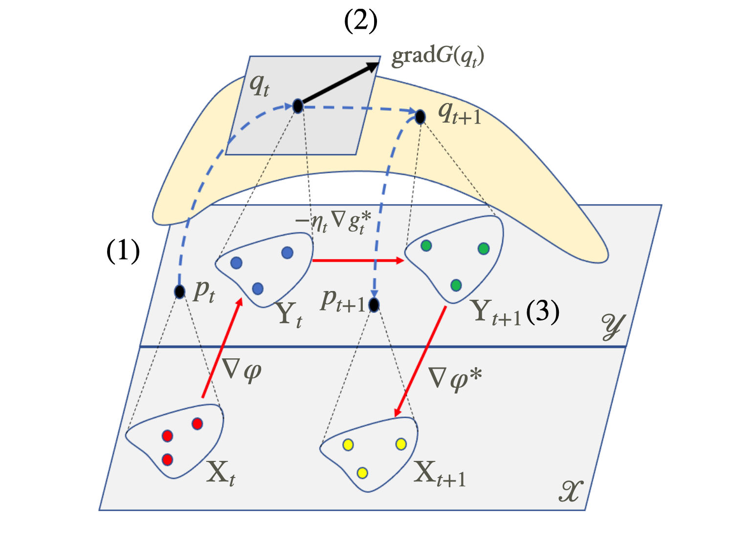
Refer to caption


Figure 1: Overview of Mirror Variational Transport (mirrorVT). In t𝑡t-th iteration, there are three main steps: (1) mirrorVT maps the particle set XtsubscriptX𝑡\textbf{X}_{t} to YtsubscriptY𝑡\textbf{Y}_{t} in the unconstrained domain 𝒴𝒴\mathcal{Y} via the mirror map φ𝜑\nabla\varphi, (2) mirrorVT pushes the particle set YtsubscriptY𝑡\textbf{Y}_{t} along the direction gtsubscriptsuperscript𝑔𝑡\nabla g^{*}_{t} in the domain 𝒴𝒴\mathcal{Y} to obtain the updated particle set Yt+1subscriptY𝑡1\textbf{Y}_{t+1}, and (3) mirrorVT maps Yt+1subscriptY𝑡1\textbf{Y}_{t+1} back to Xt+1subscriptX𝑡1\textbf{X}_{t+1} in the constrained domain 𝒳𝒳\mathcal{X} via the map φsuperscript𝜑\nabla\varphi^{*}.

The advantages of defining the functional G𝐺G on the unconstrained domain 𝒴𝒴\mathcal{Y} are as follows: 1) G𝐺G is defined over the unconstrained domain 𝒴𝒴\mathcal{Y}, which enables to apply VP to optimize G𝐺G in the dual space; 2) It is straightforward to verify the following connection between F𝐹F and G𝐺G: G/q=gq𝐺𝑞superscriptsubscript𝑔𝑞\partial G/\partial q=g_{q}^{*} and gq(y)=2φ(x)1fp(x)superscriptsubscript𝑔𝑞ysuperscript2𝜑superscriptx1superscriptsubscript𝑓𝑝x\nabla g_{q}^{*}(\textbf{y})=\nabla^{2}\varphi(\textbf{x})^{-1}\nabla f_{p}^{*}(\textbf{x}), where fpsuperscriptsubscript𝑓𝑝f_{p}^{*} and gqsuperscriptsubscript𝑔𝑞g_{q}^{*} are the optimal solutions to the variational maximization problem (13) of F𝐹F and G𝐺G, respectively.

So we propose the mirrored variational transport (mirrorVT) algorithm, as illustrated in Fig. 1, to optimize the functional F𝐹F. Initially, a set of particles X1={x1,i}i[N]subscriptX1subscriptsubscriptx1𝑖𝑖delimited-[]𝑁\textbf{X}_{1}=\left\{\textbf{x}_{1,i}\right\}_{i\in[N]} is obtained by drawing N𝑁N i.i.d observations from the initial probability distribution p1subscript𝑝1p_{1}. In each iteration t𝑡t, we maintain two set of N𝑁N particles Xt={xt,i}i[N]subscriptX𝑡subscriptsubscriptx𝑡𝑖𝑖delimited-[]𝑁\textbf{X}_{t}=\left\{\textbf{x}_{t,i}\right\}_{i\in[N]} and Yt={yt,i}i[N]subscriptY𝑡subscriptsubscripty𝑡𝑖𝑖delimited-[]𝑁\textbf{Y}_{t}=\left\{\textbf{y}_{t,i}\right\}_{i\in[N]} as follows. First, mirrorVT compute the solution ftsubscriptsuperscript𝑓𝑡f^{*}_{t} to (7) based on the current particle set XtsubscriptX𝑡\textbf{X}_{t}. Then, mirrorVT maps the current particle set XtsubscriptX𝑡\textbf{X}_{t} to the domain 𝒴𝒴\mathcal{Y} via the mirror map φ𝜑\nabla\varphi (see step 1 of Fig. 1):

yt,iφ(xt,i)subscripty𝑡𝑖𝜑subscriptx𝑡𝑖\displaystyle\textbf{y}_{t,i}\leftarrow\nabla\varphi(\textbf{x}_{t,i}) (14)

for all i[N]𝑖delimited-[]𝑁i\in[N]111We use [N] to indicate the list [1,2,,N]12𝑁\left[1,2,...,N\right] throughout the rest of the paper. This is to transform the optimization problem from constrained domain into the unconstrained one (𝒴𝒴\mathcal{Y}) and equivalent to pushing the empirical measure pt=1/Ni[N]δxt,isubscript𝑝𝑡1𝑁subscript𝑖delimited-[]𝑁subscript𝛿subscriptx𝑡𝑖p_{t}=1/N\sum_{i\in[N]}\delta_{\textbf{x}_{t,i}} by the push-forward measure induced by φ𝜑\nabla\varphi: qt=[φ]ptsubscript𝑞𝑡delimited-[]𝜑subscript𝑝𝑡q_{t}=\left[\nabla\varphi\right]\sharp p_{t}.

With the obtained ftsubscriptsuperscript𝑓𝑡f^{*}_{t}, we assume that 2φ(x)1ft(x)superscript2𝜑superscriptx1subscriptsuperscript𝑓𝑡x\nabla^{2}\varphi(\textbf{x})^{-1}\nabla f^{*}_{t}(\textbf{x}) is hh-Lipschitz continuous and one may verify that gt(y)subscriptsuperscript𝑔𝑡y\nabla g^{*}_{t}(\textbf{y}) is h/α𝛼h/\alpha-Lipschitz continuous222For any x,x𝒳xsuperscriptx𝒳\textbf{x},\textbf{x}^{\prime}\in\mathcal{X} and y=φ(x),y=φ(x)formulae-sequencey𝜑xsuperscripty𝜑superscriptx\textbf{y}=\nabla\varphi(\textbf{x}),\textbf{y}^{\prime}=\nabla\varphi(\textbf{x}^{\prime}), we have: gt(y)gt(y)2=2φ(x)1ft(x)2φ(x)1ft(x)2hxx2=hφ(y)φ(y)2h/αyy2subscriptdelimited-∥∥subscriptsuperscript𝑔𝑡ysubscriptsuperscript𝑔𝑡superscripty2subscriptdelimited-∥∥superscript2𝜑superscriptx1subscriptsuperscript𝑓𝑡xsuperscript2𝜑superscriptsuperscriptx1subscriptsuperscript𝑓𝑡superscriptx2subscriptdelimited-∥∥xsuperscriptx2subscriptdelimited-∥∥superscript𝜑ysuperscript𝜑superscripty2𝛼subscriptdelimited-∥∥ysuperscripty2\lVert\nabla g^{*}_{t}(\textbf{y})-\nabla g^{*}_{t}(\textbf{y}^{\prime})\rVert_{2}=\lVert\nabla^{2}\varphi(\textbf{x})^{-1}\nabla f^{*}_{t}(\textbf{x})-\nabla^{2}\varphi(\textbf{x}^{\prime})^{-1}\nabla f^{*}_{t}(\textbf{x}^{\prime})\rVert_{2}\leq h\lVert\textbf{x}-\textbf{x}^{\prime}\rVert_{2}=h\lVert\nabla\varphi^{*}(\textbf{y})-\nabla\varphi^{*}(\textbf{y}^{\prime})\rVert_{2}\leq h/\alpha\lVert\textbf{y}-\textbf{y}^{\prime}\rVert_{2}, where the last inequality holds as φsuperscript𝜑\varphi^{*} is 1/α1𝛼1/\alpha-smooth.. Hence for any ηt[0,α/h)subscript𝜂𝑡0𝛼\eta_{t}\in\left[0,\alpha/h\right), we can enable mirrorVT to push the particles in the dual domain as follows (see step 2 of Fig. 1):

yt+1,iExpyt,i{ηt2φ(xt,i)1ft(xt,i)}subscripty𝑡1𝑖subscriptExpsubscripty𝑡𝑖subscript𝜂𝑡superscript2𝜑superscriptsubscriptx𝑡𝑖1subscriptsuperscript𝑓𝑡subscriptx𝑡𝑖\displaystyle\textbf{y}_{t+1,i}\leftarrow\texttt{Exp}_{\textbf{y}_{t,i}}\left\{-\eta_{t}\nabla^{2}\varphi(\textbf{x}_{t,i})^{-1}f^{*}_{t}(\textbf{x}_{t,i})\right\} (15)

for all i[N]𝑖delimited-[]𝑁i\in[N]. This is equivalent to updating the empirical measure qt=1/Ni[N]δyt,isubscript𝑞𝑡1𝑁subscript𝑖delimited-[]𝑁subscript𝛿subscripty𝑡𝑖q_{t}=1/N\sum_{i\in[N]}\delta_{\textbf{y}_{t,i}} by the push-forward measure [Exp𝒴(ηtgt)]qtdelimited-[]subscriptExp𝒴subscript𝜂𝑡subscriptsuperscript𝑔𝑡subscript𝑞𝑡\left[\texttt{Exp}_{\mathcal{Y}}(-\eta_{t}\nabla g^{*}_{t})\right]\sharp q_{t}, which is realized by applying Proposition 3.1 in [7] for the function gtsubscriptsuperscript𝑔𝑡g^{*}_{t} defined over the dual domain 𝒴𝒴\mathcal{Y}. At the end of t𝑡t-th iteration, mirrorVT maps particles back to the original constrained domain 𝒳𝒳\mathcal{X} (see step 3 of Fig. 1):

xt+1,iφ(yt+1,i)subscriptx𝑡1𝑖superscript𝜑subscripty𝑡1𝑖\displaystyle\textbf{x}_{t+1,i}\leftarrow\nabla\varphi^{*}(\textbf{y}_{t+1,i}) (16)

for all i[N]𝑖delimited-[]𝑁i\in[N]. This step is equivalent to pushing the updated empirical measure qt+1=1/Ni[N]δyt+1,isubscript𝑞𝑡11𝑁subscript𝑖delimited-[]𝑁subscript𝛿subscripty𝑡1𝑖q_{t+1}=1/N\sum_{i\in[N]}\delta_{\textbf{y}_{t+1,i}} from the dual domain to the primal one by the push-forward measure [φ]qt+1delimited-[]superscript𝜑subscript𝑞𝑡1\left[\nabla\varphi^{*}\right]\sharp q_{t+1}.

4.2 Continuous-time dynamics of ptsubscript𝑝𝑡p_{t}

We can view steps of mirrorVT as a discretization of the following continuous-time dynamics of particles (as ηt0subscript𝜂𝑡0\eta_{t}\rightarrow 0):

dyt=2φ(xt)1ft(xt)dt and xt=φ(yt)dtdsubscripty𝑡superscript2𝜑superscriptsubscriptx𝑡1subscriptsuperscript𝑓𝑡subscriptx𝑡d𝑡subscript and x𝑡superscript𝜑subscripty𝑡d𝑡\mathrm{d}\textbf{y}_{t}=-\nabla^{2}\varphi(\textbf{x}_{t})^{-1}\nabla f^{*}_{t}(\textbf{x}_{t})\mathrm{d}t\text{ and }\textbf{x}_{t}=\nabla\varphi^{*}(\textbf{y}_{t})\mathrm{d}t (17)

which is equivalent to

dxtdt=(xtyt)1dytdt=2φ(xt)2ft(xt)dsubscriptx𝑡d𝑡superscriptsubscriptsubscriptx𝑡subscripty𝑡1dsubscripty𝑡d𝑡superscript2𝜑superscriptsubscriptx𝑡2subscriptsuperscript𝑓𝑡subscriptx𝑡\frac{\mathrm{d}\textbf{x}_{t}}{\mathrm{d}t}=\left(\nabla_{\textbf{x}_{t}}\textbf{y}_{t}\right)^{-1}\frac{\mathrm{d}\textbf{y}_{t}}{\mathrm{d}t}=-\nabla^{2}\varphi(\textbf{x}_{t})^{-2}\nabla f^{*}_{t}(\textbf{x}_{t}) (18)

by applying the chain rule. We now consider the continuous-time dynamic of ptsubscript𝑝𝑡p_{t} and its limit. Let γt:+𝒫2(𝒳):subscript𝛾𝑡superscriptsubscript𝒫2𝒳\gamma_{t}:\mathbb{R}^{+}\rightarrow\mathcal{P}_{2}(\mathcal{X}) be a curve with probability measures ptsubscript𝑝𝑡p_{t}, vt(xt)subscript𝑣𝑡subscriptx𝑡v_{t}(\textbf{x}_{t}) be the vector field which satisfy the continuity equation: tpt=div(ptvt)subscript𝑡subscript𝑝𝑡divsubscript𝑝𝑡subscript𝑣𝑡\partial_{t}p_{t}=-\texttt{div}(p_{t}v_{t}). As shown in the following Proposition 1, the functional F𝐹F is decreasing along the curve γtsubscript𝛾𝑡\gamma_{t}. Let psuperscript𝑝p^{*} be the optimal solution of F𝐹F and assume F𝐹F is geodesically convex, the limit of ptsubscript𝑝𝑡p_{t} is psuperscript𝑝p^{*} as t𝑡t\rightarrow\infty.

Proposition 1.

F(pt)𝐹subscript𝑝𝑡F(p_{t}) is decreasing in time and satisfies:

dF(pt)dt=𝔼xpt2φ(x)1ft(x)220d𝐹subscript𝑝𝑡d𝑡subscript𝔼similar-toxsubscript𝑝𝑡subscriptsuperscriptdelimited-∥∥superscript2𝜑superscriptx1subscriptsuperscript𝑓𝑡x220\displaystyle\frac{\mathrm{d}F(p_{t})}{\mathrm{d}t}=-\mathbb{E}_{\textbf{x}\sim p_{t}}\lVert\nabla^{2}\varphi(\textbf{x})^{-1}\nabla f^{*}_{t}(\textbf{x})\rVert^{2}_{2}\leq 0 (19)
Proof.

The proof can be obtained by the following calculation:

dF(pt)dtd𝐹subscript𝑝𝑡d𝑡\displaystyle\frac{\mathrm{d}F(p_{t})}{\mathrm{d}t} =F(pt)ptptt=F(pt)ptdiv(ptvt)absent𝐹subscript𝑝𝑡subscript𝑝𝑡subscript𝑝𝑡𝑡𝐹subscript𝑝𝑡subscript𝑝𝑡divsubscript𝑝𝑡subscript𝑣𝑡\displaystyle=\int\frac{\partial F(p_{t})}{\partial p_{t}}\frac{\partial p_{t}}{\partial t}=-\int\frac{\partial F(p_{t})}{\partial p_{t}}\texttt{div}(p_{t}v_{t})
=F(pt)pt(x),vt(x)pt(x)dx=ft(x),vt(x)pt(x)dxabsent𝐹subscript𝑝𝑡subscript𝑝𝑡xsubscript𝑣𝑡xsubscript𝑝𝑡xdifferential-dxsubscriptsuperscript𝑓𝑡xsubscript𝑣𝑡xsubscript𝑝𝑡xdifferential-dx\displaystyle=\int\langle\nabla\frac{\partial F(p_{t})}{\partial p_{t}}(\textbf{x}),v_{t}(\textbf{x})\rangle p_{t}(\textbf{x})\mathrm{d}\textbf{x}=\int\langle\nabla f^{*}_{t}(\textbf{x}),v_{t}(\textbf{x})\rangle p_{t}(\textbf{x})\mathrm{d}\textbf{x}
=ft(x),2φ(x)2ft(x)pt(x)dx=ft(x),2φ(x)2ft(x)pt(x)dxabsentsubscriptsuperscript𝑓𝑡xsuperscript2𝜑superscriptx2subscriptsuperscript𝑓𝑡xsubscript𝑝𝑡xdifferential-dxsubscriptsuperscript𝑓𝑡xsuperscript2𝜑superscriptx2subscriptsuperscript𝑓𝑡xsubscript𝑝𝑡xdifferential-dx\displaystyle=-\int\langle\nabla f^{*}_{t}(\textbf{x}),\nabla^{2}\varphi(\textbf{x})^{-2}\nabla f^{*}_{t}(\textbf{x})\rangle p_{t}(\textbf{x})\mathrm{d}\textbf{x}=-\int\langle\nabla f^{*}_{t}(\textbf{x}),\nabla^{2}\varphi(\textbf{x})^{-2}\nabla f^{*}_{t}(\textbf{x})\rangle p_{t}(\textbf{x})\mathrm{d}\textbf{x}
=𝔼xpt2φ(x)1ft(x)22absentsubscript𝔼similar-toxsubscript𝑝𝑡subscriptsuperscriptdelimited-∥∥superscript2𝜑superscriptx1subscriptsuperscript𝑓𝑡x22\displaystyle=-\mathbb{E}_{\textbf{x}\sim p_{t}}\lVert\nabla^{2}\varphi(\textbf{x})^{-1}\nabla f^{*}_{t}(\textbf{x})\rVert^{2}_{2}

where the equality in the first line is obtained by the definition of continuity equation, the equality in the second line is obtained by Equation (5) and Proposition 3.1 in [7], and the equality in the third line is obtained by Equation (18). The proof is completed. ∎

4.3 Relation to Stein Variational Mirror Descent [12]

Stein Variational Mirror Descent (SVMD, [12]), most related to Algorithm 2, minimizes the KL divergence to the target distribution defined over a constrained domain by pushing particles in the dual space induced by a mirror map. In what follows, we verify that mirrorVT when using KL-divergence as the objective functional relates to SVMD algorithms via the integral operator. First we give the definition of the integral operator as follows:

Definition 1.

(Integral operator, [10]) Let k:𝒳×𝒳:𝑘𝒳𝒳k:\mathcal{X}\times\mathcal{X}\rightarrow\mathbb{R} be a reproducing kernel, 𝒳𝒳\mathcal{X} is endowed with a probability measure p𝑝p, L2(𝒳,p)superscript𝐿2𝒳𝑝L^{2}(\mathcal{X},p) be the space of square integrable functions with norm fp2=f,fp=|f(x)|2dp(x)superscriptsubscriptdelimited-∥∥𝑓𝑝2subscript𝑓𝑓𝑝superscript𝑓x2differential-d𝑝x\lVert f\rVert_{p}^{2}=\langle f,f\rangle_{p}=\int|f(\textbf{x})|^{2}\mathrm{d}p(\textbf{x}). We define k,p:L2(𝒳,p)L2(𝒳,p):subscript𝑘𝑝superscript𝐿2𝒳𝑝superscript𝐿2𝒳𝑝\mathcal{L}_{k,p}:L^{2}(\mathcal{X},p)\rightarrow L^{2}(\mathcal{X},p) to be the corresponding integral operator given by:

k,pf(x)=𝒳k(x,x)f(x)p(x)dxsubscript𝑘𝑝𝑓xsubscript𝒳𝑘xsuperscriptx𝑓superscriptx𝑝superscriptxdifferential-dx\displaystyle\mathcal{L}_{k,p}f(\textbf{x})=\int_{\mathcal{X}}k(\textbf{x},\textbf{x}^{\prime})f(\textbf{x}^{\prime})p(\textbf{x}^{\prime})\mathrm{d}\textbf{x} (20)

The following theorem shows the connection between mirrorVP and SVMD.

Theorem 2.

Let F(p)=KL(p||p)F(p)=\text{KL}(p||p^{*}), for p𝒫2(𝒳)𝑝subscript𝒫2𝒳p\in\mathcal{P}_{2}(\mathcal{X}) be the functional to be optimized, k𝑘k be the reproducing kernel defined on 𝒳𝒳\mathcal{X}, kφ(y,y)=k(φ(y),φ(y))subscript𝑘𝜑ysuperscripty𝑘superscript𝜑ysuperscript𝜑superscriptyk_{\varphi}(\textbf{y},\textbf{y}^{\prime})=k(\nabla\varphi^{*}(\textbf{y}),\nabla\varphi^{*}(\textbf{y}^{\prime})) for y,y𝒴ysuperscripty𝒴\textbf{y},\textbf{y}^{\prime}\in\mathcal{Y}. In t𝑡t-th iteration, the integral operator k,ptsubscript𝑘subscript𝑝𝑡\mathcal{L}_{k,p_{t}} applied on the update direction vtsubscript𝑣𝑡v_{t} is given by:

k,ptvt(x)=𝔼yqtkφ(y,y)logq(y)+ykφ(y,y)x𝒳,y=φ(x)𝒴formulae-sequencesubscript𝑘subscript𝑝𝑡subscript𝑣𝑡xsubscript𝔼similar-tosuperscriptysubscript𝑞𝑡subscript𝑘𝜑ysuperscriptysuperscript𝑞superscriptysubscriptysubscript𝑘𝜑ysuperscriptyfor-allsuperscriptx𝒳superscripty𝜑superscriptx𝒴\mathcal{L}_{k,p_{t}}v_{t}(\textbf{x})=-\mathbb{E}_{\textbf{y}^{\prime}\sim q_{t}}k_{\varphi}(\textbf{y},\textbf{y}^{\prime})\nabla\log q^{*}(\textbf{y}^{\prime})+\nabla_{\textbf{y}}k_{\varphi}(\textbf{y},\textbf{y}^{\prime})\text{, }\forall\textbf{x}^{\prime}\in\mathcal{X},\textbf{y}^{\prime}=\nabla\varphi(\textbf{x}^{\prime})\in\mathcal{Y} (21)

The proof of Theorem 2 is given in Appendix A.1. We could observe that the right-hand side of (21) is the same as that of (11) in [12], suggesting that in case that we optimize the KL-divergence and approximate the optimal update direction in the dual space by kernel k𝑘k through the integral operator, mirrorVT reduces to SVMD. Especially, when k(x,x)=1𝑘xsuperscriptx1k(\textbf{x},\textbf{x}^{\prime})=1 if x=xxsuperscriptx\textbf{x}=\textbf{x}^{\prime} and 0 otherwise, mirrorVT exactly recovers SVMD, so we could say that SVMD is a special case of mirrorVT. However, it might be challenging to derive a similar kernel-based update for divergences beyond KL-divergence.

Input: Functional F𝐹F, number of particles N𝑁N, number of iterations: K𝐾K, and initial weights w(0)w0\textbf{w}(0)
Output: fw^subscript𝑓^wf_{\hat{\textbf{w}}}
1 Stepsize η=N1/2𝜂superscript𝑁12\eta=N^{-1/2}
2 s0𝑠0s\leftarrow 0
3 while s<N𝑠𝑁s<N do
       x=xs+1xsubscriptx𝑠1\textbf{x}=\textbf{x}_{s+1} ;
       // pick up a sample
       gw(s)(x)θF(fw(s)(x))wfw(s)(x)subscript𝑔w𝑠xsubscript𝜃superscript𝐹subscript𝑓w𝑠xsubscriptwsubscript𝑓w𝑠xg_{\textbf{w}(s)}(\textbf{x})\leftarrow\nabla_{\theta}F^{*}(f_{\textbf{w}(s)}(\textbf{x}))-\nabla_{\textbf{w}}f_{\textbf{w}(s)}(\textbf{x}) ;
       // compute gradient w.r.t network parameters
       w(s+1/2)w(s)ηgw(s)(x)w𝑠12w𝑠𝜂subscript𝑔w𝑠x\textbf{w}(s+1/2)\leftarrow\textbf{w}(s)-\eta g_{\textbf{w}(s)}(\textbf{x});
       // update network parameters
       w(s+1)argminw0{ww(s+1/2)2}w𝑠1subscriptargminwsuperscript0subscriptdelimited-∥∥ww𝑠122\textbf{w}(s+1)\leftarrow\mathop{\rm arg~{}min}\limits_{\textbf{w}\in\mathcal{B}^{0}}\left\{\lVert\textbf{w}-\textbf{w}(s+1/2)\rVert_{2}\right\};
       // guarantee to lie in the ball 0(rf)superscript0subscript𝑟𝑓\mathcal{B}^{0}(r_{f})
4       ss+1𝑠𝑠1s\leftarrow s+1
5 end while
w^=1/Ns=0N1w(s)^w1𝑁superscriptsubscript𝑠0𝑁1w𝑠\hat{\textbf{w}}=1/N\cdot\sum_{s=0}^{N-1}\textbf{w}(s)
Algorithm 1 Variational Form Maximization (VFM({xi}i[N]subscriptsubscriptx𝑖𝑖delimited-[]𝑁\left\{\textbf{x}_{i}\right\}_{i\in[N]}, F𝐹F))

4.4 Convergence Analysis

In this section, we analyze the convergence of mirrorVT. Its pseudocode is shown in Algorithm 2.

In practice, we need to solve the empirical variational maximization problem (9) with finite samples via stochastic gradient descent to get the estimate ft~~subscriptsuperscript𝑓𝑡\tilde{f^{*}_{t}} of the true ftsubscriptsuperscript𝑓𝑡f^{*}_{t} (see Algorithm 1). The true Wasserstein gradient at ptsubscript𝑝𝑡p_{t} is given by gradF(pt)=div(ptft)grad𝐹subscript𝑝𝑡divsubscript𝑝𝑡subscriptsuperscript𝑓𝑡\texttt{grad}F(p_{t})=-\texttt{div}(p_{t}\nabla f^{*}_{t}) and its estimate is given by div(ptft~)divsubscript𝑝𝑡~superscriptsubscript𝑓𝑡-\texttt{div}(p_{t}\nabla\tilde{f_{t}^{*}}), so the difference is given by δt=div(pt(ft~ft))subscript𝛿𝑡divsubscript𝑝𝑡~superscriptsubscript𝑓𝑡subscriptsuperscript𝑓𝑡\delta_{t}=-\texttt{div}(p_{t}(\nabla\tilde{f_{t}^{*}}-\nabla f^{*}_{t})). Hence, the expected gradient error is defined as:

ϵt=𝔼δt,δtpt=𝔼ft~(x)ft(x)22pt(x)dxsubscriptitalic-ϵ𝑡𝔼subscriptsubscript𝛿𝑡subscript𝛿𝑡subscript𝑝𝑡𝔼subscriptsuperscriptdelimited-∥∥~superscriptsubscript𝑓𝑡xsubscriptsuperscript𝑓𝑡x22subscript𝑝𝑡xdifferential-dx\displaystyle\epsilon_{t}=\mathbb{E}\langle\delta_{t},\delta_{t}\rangle_{p_{t}}=\mathbb{E}\int\lVert\nabla\tilde{f_{t}^{*}}(\textbf{x})-\nabla f^{*}_{t}(\textbf{x})\rVert^{2}_{2}p_{t}(\textbf{x})\mathrm{d}\textbf{x} (22)

where the expectation is taken over the initial particles. To derive the upper bound of ϵtsubscriptitalic-ϵ𝑡\epsilon_{t}, according to [7], we assume to learn the function ft~~superscriptsubscript𝑓𝑡\tilde{f_{t}^{*}} from the class ~~\tilde{\mathcal{F}} of neural networks (10). The gradient error, defined in (22), is upper bounded by: O(rf2/N1/2+rf3/nw1/2+rf4/nw)𝑂superscriptsubscript𝑟𝑓2superscript𝑁12superscriptsubscript𝑟𝑓3superscriptsubscript𝑛𝑤12superscriptsubscript𝑟𝑓4subscript𝑛𝑤O\left(r_{f}^{2}/N^{1/2}+r_{f}^{3}/n_{w}^{1/2}+r_{f}^{4}/n_{w}\right). See [7] for the assumptions and proofs. It is noted that the gradient error decays to zero at the rate of 1/N1𝑁1/\sqrt{N} with a sufficiently large width nwsubscript𝑛𝑤n_{w} of the neural network. Furthermore, the order of gradient error is independent of the iteration t𝑡t.

We further make the following assumptions on the functionals F𝐹F and G𝐺G (see [7] for the reference) to analyze the convergence of Algorithm 2.

Input: Functional F:𝒫2(𝒳):𝐹subscript𝒫2𝒳F:\mathcal{P}_{2}(\mathcal{X})\rightarrow\mathbb{R}, initial measure p1𝒫2(𝒳)subscript𝑝1subscript𝒫2𝒳p_{1}\in\mathcal{P}_{2}(\mathcal{X}), number of particles N𝑁N, number of iterations: T𝑇T and stepsizes {ηt}t=1Tsuperscriptsubscriptsubscript𝜂𝑡𝑡1𝑇\left\{\eta_{t}\right\}_{t=1}^{T}.
Output: The final set of particles XTsubscriptX𝑇\textbf{X}_{T}
1 Generate N𝑁N particles X1={x1,i}i[N]subscriptX1subscriptsubscriptx1𝑖𝑖delimited-[]𝑁\textbf{X}_{1}=\left\{\textbf{x}_{1,i}\right\}_{i\in[N]} by drawing N𝑁N i.i.d. observations from p1subscript𝑝1p_{1}.
2 while tT𝑡𝑇t\leq T do
       ft~VFM(Xt,F)~superscriptsubscript𝑓𝑡VFMsubscriptX𝑡𝐹\tilde{f_{t}^{*}}\leftarrow\textbf{VFM}(\textbf{X}_{t},F);
       // estimate solution of variational maximization problem
       for i[N]𝑖delimited-[]𝑁i\in[N]\text{: }yt,iφ(xt,i)subscripty𝑡𝑖𝜑subscriptx𝑡𝑖\textbf{y}_{t,i}\leftarrow\nabla\varphi(\textbf{x}_{t,i}) ;
       // map particles into the dual space
       for i[N]𝑖delimited-[]𝑁i\in[N]\text{: }vt(xt,i)2φ(xt,i)1ft~(xt,i)subscript𝑣𝑡subscriptx𝑡𝑖superscript2𝜑superscriptsubscriptx𝑡𝑖1~superscriptsubscript𝑓𝑡subscriptx𝑡𝑖v_{t}(\textbf{x}_{t,i})\leftarrow\nabla^{2}\varphi(\textbf{x}_{t,i})^{-1}\nabla\tilde{f_{t}^{*}}(\textbf{x}_{t,i});
       // calculate update direction for each particle
       for i[N]𝑖delimited-[]𝑁i\in[N]\text{: }yt+1,iyt,iηtvt(xt,i)subscripty𝑡1𝑖subscripty𝑡𝑖subscript𝜂𝑡subscript𝑣𝑡subscriptx𝑡𝑖\textbf{y}_{t+1,i}\leftarrow\textbf{y}_{t,i}-\eta_{t}v_{t}(\textbf{x}_{t,i});
       // push each particle in dual space
       for i[N]𝑖delimited-[]𝑁i\in[N]\text{: }xt+1,iφ(yt+1,i)subscriptx𝑡1𝑖superscript𝜑subscripty𝑡1𝑖\textbf{x}_{t+1,i}\leftarrow\nabla\varphi^{*}(\textbf{y}_{t+1,i});
       // map updated particle to primal space
       Xt+1{xt+1,i}i[N]subscriptX𝑡1subscriptsubscriptx𝑡1𝑖𝑖delimited-[]𝑁\textbf{X}_{t+1}\leftarrow\left\{\textbf{x}_{t+1,i}\right\}_{i\in[N]};
       // update particle set
3       tt+1𝑡𝑡1t\leftarrow t+1
4 end while
Algorithm 2 The Mirrored Variational Transport (mirrorVT) algorithm

Assumption 1.1 (Geodesic smoothness). We assume that F𝐹F and G𝐺G are geodesically L1subscript𝐿1L_{1}- and L2subscript𝐿2L_{2}-smooth with respect to the 222-Wasserstein distance in the sense that: for pfor-all𝑝\forall p, p𝒫2(𝒳)superscript𝑝subscript𝒫2𝒳p^{\prime}\in\mathcal{P}_{2}(\mathcal{X}), qfor-all𝑞\forall q, q𝒫2(𝒴)superscript𝑞subscript𝒫2𝒴q^{\prime}\in\mathcal{P}_{2}(\mathcal{Y}):

F(p)𝐹superscript𝑝\displaystyle F(p^{\prime}) F(p)+gradF(p),Expp1(p)p+L12𝒲22(p,p)absent𝐹𝑝subscriptgrad𝐹𝑝superscriptsubscriptExp𝑝1superscript𝑝𝑝subscript𝐿12subscriptsuperscript𝒲22superscript𝑝𝑝\displaystyle\leq F(p)+\langle\texttt{grad}F(p),\texttt{Exp}_{p}^{-1}(p^{\prime})\rangle_{p}+\frac{L_{1}}{2}\cdot\mathcal{W}^{2}_{2}(p^{\prime},p) (23)
G(q)𝐺superscript𝑞\displaystyle G(q^{\prime}) G(q)+gradG(q),Expq1(q)q+L22𝒲22(q,q)absent𝐺𝑞subscriptgrad𝐺𝑞superscriptsubscriptExp𝑞1superscript𝑞𝑞subscript𝐿22subscriptsuperscript𝒲22superscript𝑞𝑞\displaystyle\leq G(q)+\langle\texttt{grad}G(q),\texttt{Exp}_{q}^{-1}(q^{\prime})\rangle_{q}+\frac{L_{2}}{2}\cdot\mathcal{W}^{2}_{2}(q^{\prime},q) (24)

We also assume that F𝐹F is geodesically μ𝜇\mu-strongly convex with respect to the 222-Wasserstein distance. That is:

Assumption 1.2 (Geodesic strong convexity) for pfor-all𝑝\forall p, p𝒫2(𝒳)superscript𝑝subscript𝒫2𝒳p^{\prime}\in\mathcal{P}_{2}(\mathcal{X}), we have:

F(p)𝐹superscript𝑝\displaystyle F(p^{\prime}) F(p)+gradF(p),Expp1(p)p+μ2𝒲22(p,p)absent𝐹𝑝subscriptgrad𝐹𝑝superscriptsubscriptExp𝑝1superscript𝑝𝑝𝜇2subscriptsuperscript𝒲22superscript𝑝𝑝\displaystyle\geq F(p)+\langle\texttt{grad}F(p),\texttt{Exp}_{p}^{-1}(p^{\prime})\rangle_{p}+\frac{\mu}{2}\cdot\mathcal{W}^{2}_{2}(p^{\prime},p) (25)

The geodesic strong convexity of F𝐹F ensures that it admits the gradient dominance defined as follows:

Assumption 1.3 (μ𝜇\mu-gradient dominance) for F𝐹F satisfying (25) is gradient dominated in the sense that:

μ(F(pt)F(p))gradF(p),gradF(p)p𝜇𝐹subscript𝑝𝑡𝐹superscript𝑝subscriptgrad𝐹𝑝grad𝐹𝑝𝑝\displaystyle\mu\cdot\left(F(p_{t})-F(p^{*})\right)\leq\langle\texttt{grad}F(p),\texttt{grad}F(p)\rangle_{p} (26)
Theorem 3.

(Convergence of Algorithm 2) Let the metric tensor 0αI2φ(x)βIprecedes0𝛼Iprecedes-or-equalssuperscript2𝜑xprecedes-or-equals𝛽I0\prec\alpha\textbf{I}\preceq\nabla^{2}\varphi(\textbf{x})\preceq\beta\textbf{I} for all x𝒳x𝒳\textbf{x}\in\mathcal{X} and under the Assumptions 1.1 and 1.2, for t𝑡t-th iteration of Algorithm 2 with the constant stepsize η(0,min{1/4L1,α/h,1/μβ2})𝜂014subscript𝐿1𝛼1𝜇superscript𝛽2\eta\in\left(0,\min\left\{1/4L_{1},\alpha/h,1/\mu\beta^{2}\right\}\right), it holds that:

𝔼[F(pt+1)]infp𝒫2(𝒳)F(p)ρt(𝔼[F(p1)]infp𝒫2(𝒳)F(p))+1ρt1ρηα2Error𝔼delimited-[]𝐹subscript𝑝𝑡1subscriptinfimum𝑝subscript𝒫2𝒳𝐹𝑝superscript𝜌𝑡𝔼delimited-[]𝐹subscript𝑝1subscriptinfimum𝑝subscript𝒫2𝒳𝐹𝑝1superscript𝜌𝑡1𝜌𝜂superscript𝛼2Error\displaystyle\mathbb{E}\left[F(p_{t+1})\right]-\inf_{p\in\mathcal{P}_{2}(\mathcal{X})}F(p)\leq\rho^{t}\left(\mathbb{E}\left[F(p_{1})\right]-\inf_{p\in\mathcal{P}_{2}(\mathcal{X})}F(p)\right)+\frac{1-\rho^{t}}{1-\rho}\frac{\eta}{\alpha^{2}}\cdot\texttt{Error} (27)

where ρ=1μη/2β2[0,1]𝜌1𝜇𝜂2superscript𝛽201\rho=1-\mu\eta/2\beta^{2}\in\left[0,1\right] is the contraction factor, Error=O(rf2/N1/2+rf3/nw1/2+rf4/nw)Error𝑂superscriptsubscript𝑟𝑓2superscript𝑁12superscriptsubscript𝑟𝑓3superscriptsubscript𝑛𝑤12superscriptsubscript𝑟𝑓4subscript𝑛𝑤\texttt{Error}=O\left(r_{f}^{2}/N^{1/2}+r_{f}^{3}/n_{w}^{1/2}+r_{f}^{4}/n_{w}\right) is the gradient error and the expectation is taken over the initial particle set.

The proof of Theorem 3 is given in the Appendix A.2. It is noted that in (27) there are optimization and gradient errors. The optimization error linearly decays by the factor of ρ𝜌\rho, while statistical gradient error decays at the rate of 1/N1𝑁1/\sqrt{N} (N𝑁N is number of particles).

5 Experiments

In this section, we conduct a series of simulated experiments to assess algorithms for optimizing functionals with respect to the distributions defined over the constrained domain. The functionals take the forms of KL-divergence, JS-divergence and Wasserstein distance characterizing the distances to the the target distributions psuperscript𝑝p^{*}.

5.1 Case studies on synthetic data

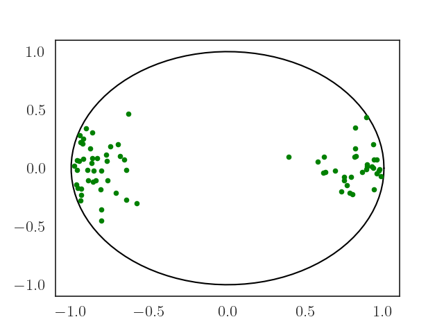
We consider two case studies with a truncated distribution and a composition distribution. For the first case, we consider an example of two-components Gaussian mixture truncated in a unit ball d={xd:x21}superscript𝑑conditional-setxsuperscript𝑑subscriptdelimited-∥∥x21\mathcal{B}^{d}=\left\{\textbf{x}\in\mathbb{R}^{d}:\lVert\textbf{x}\rVert_{2}\leq 1\right\}. We generate 100 two-dimensional samples for each Gaussian component and throw away samples outside the unit ball and use the remaining ones to represent the target distribution psuperscript𝑝p^{*} (see Fig. 2 left). The two Gaussian components are characterized by the following means and variances: μ1=[1,0],μ2=[1,0],σ1=σ2=0.2formulae-sequencesubscript𝜇110formulae-sequencesubscript𝜇210subscript𝜎1subscript𝜎20.2\mu_{1}=\left[-1,0\right],\mu_{2}=\left[1,0\right],\sigma_{1}=\sigma_{2}=0.2.

Refer to caption
(a) Samples from two-components Gaussian mixture truncated by the unit ball.
Refer to caption
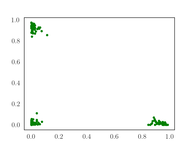
(b) Samples from three-components Dirichlet mixture.
Figure 2: Ground truth samples.

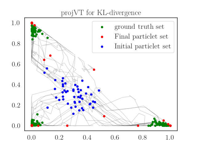
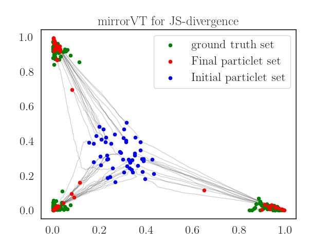
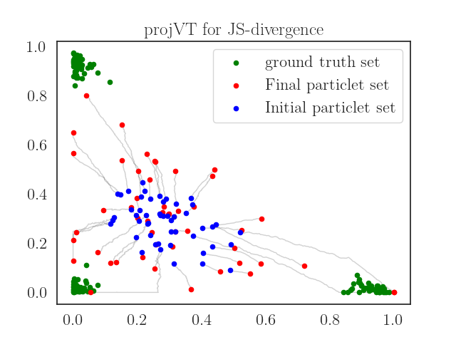
For the second case, we consider an example of composition distribution defined on a simplex Δd={x0d:i=1dxi=1}superscriptΔ𝑑conditional-setxsuperscriptsubscriptabsent0𝑑superscriptsubscript𝑖1𝑑subscriptx𝑖1\Delta^{d}=\left\{\textbf{x}\in\mathbb{R}_{\geq 0}^{d}:\sum_{i=1}^{d}\textbf{x}_{i}=1\right\}. In particular, we consider three-components Dirichlet mixture (see Fig. 2 right). We generate 50 five-dimensional samples for each component. The Dirichlet distribution with unnormalized density of the form p(x)i=1dxiαi1,xΔdformulae-sequenceproportional-to𝑝xsuperscriptsubscriptproduct𝑖1𝑑superscriptsubscriptx𝑖subscript𝛼𝑖1for-allxsuperscriptΔ𝑑p(\textbf{x})\propto\prod_{i=1}^{d}\textbf{x}_{i}^{\alpha_{i}-1},\forall\textbf{x}\in\Delta^{d}, is characterized by the concentration parameters αi0,i[d]formulae-sequencesubscript𝛼𝑖0𝑖delimited-[]𝑑\alpha_{i}\geq 0,i\in[d]. The three Dirichlet components in the simulation are characterized by α1=[50,1,1,1,1]superscript𝛼1501111\alpha^{1}=[50,1,1,1,1], α2=[1,50,1,1,1]superscript𝛼2150111\alpha^{2}=[1,50,1,1,1] and α3=[1,1,50,1,1]superscript𝛼3115011\alpha^{3}=[1,1,50,1,1]. By visualizing only two first coordinates of data point samples, we can see that samples are mainly concentrated on three corners. For truncated Gaussian mixture, we generate 100 samples as the initial particle set which represents the initial measure p1subscript𝑝1p_{1} (see Algorithm 2). For Dirichlet mixture, we generate 50 samples from the Dirichlet distribution characterized by α=[5,5,5,5,5]𝛼55555\alpha=[5,5,5,5,5].

Refer to caption
Refer to caption
Refer to caption
Refer to caption
Refer to caption
Refer to caption
Refer to caption
Refer to caption
Refer to caption
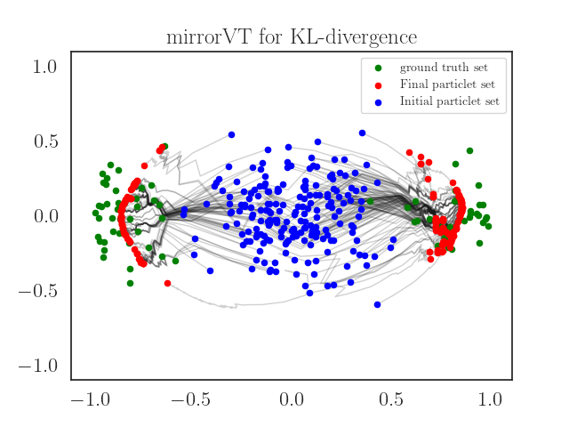
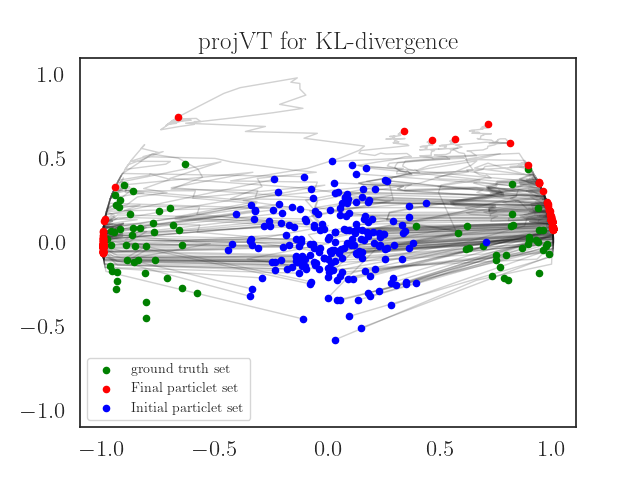
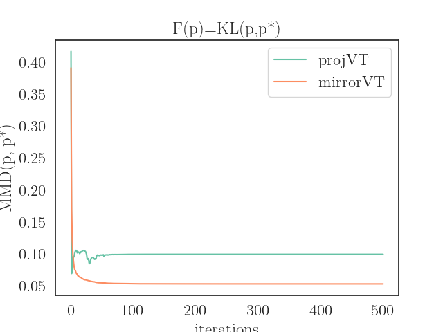
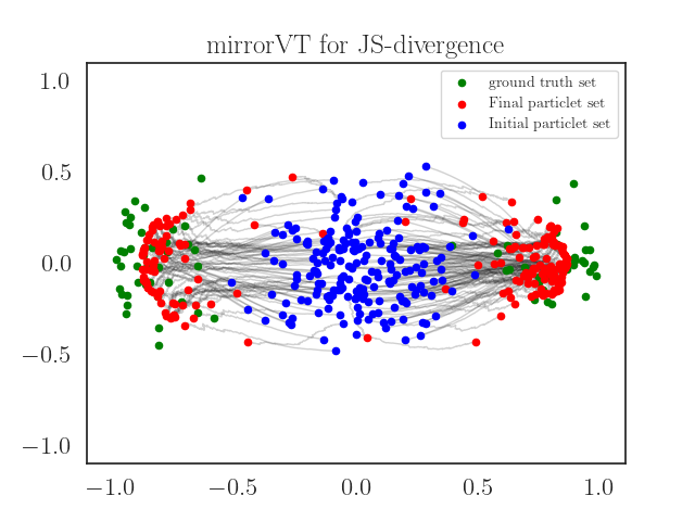
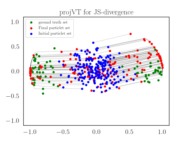
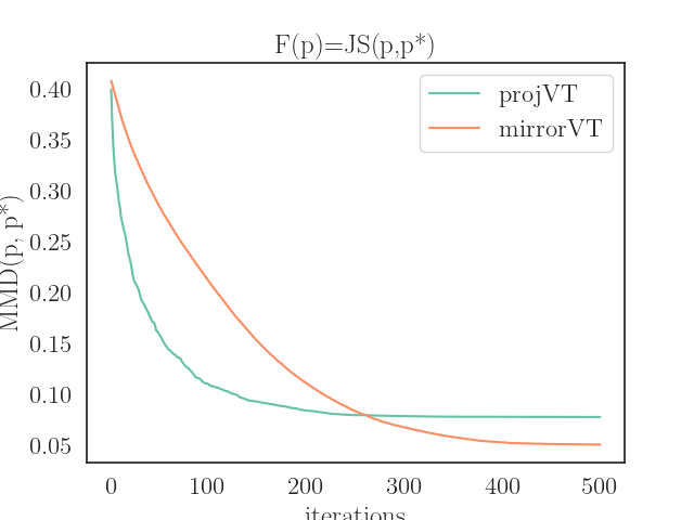
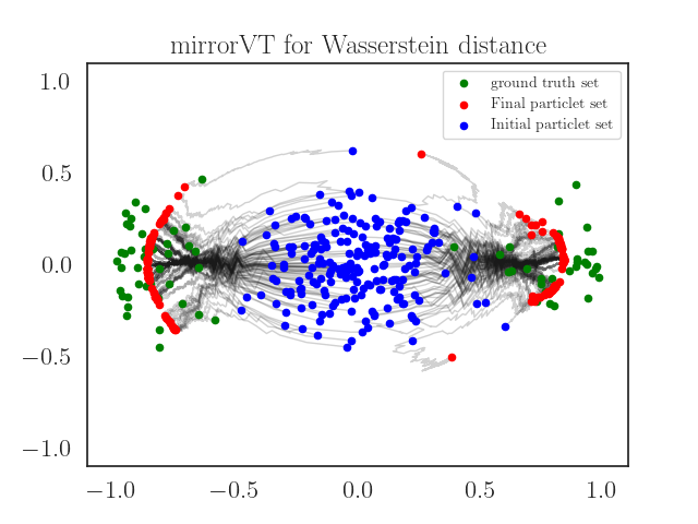
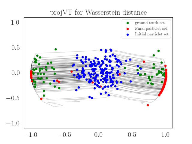
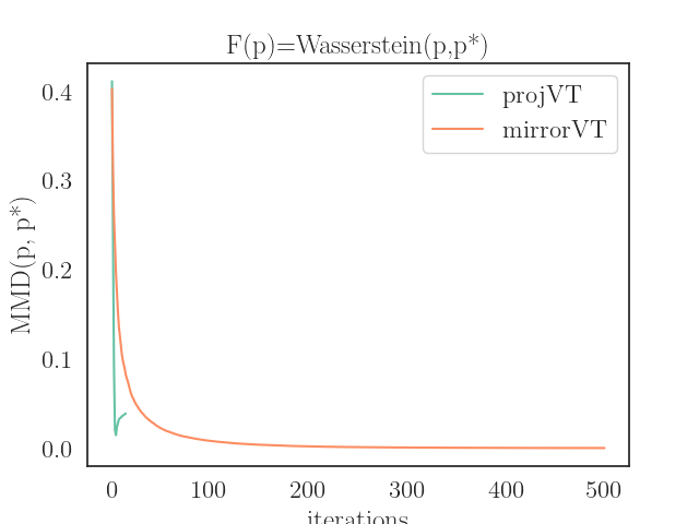
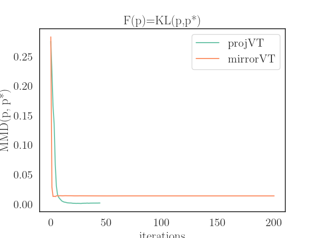
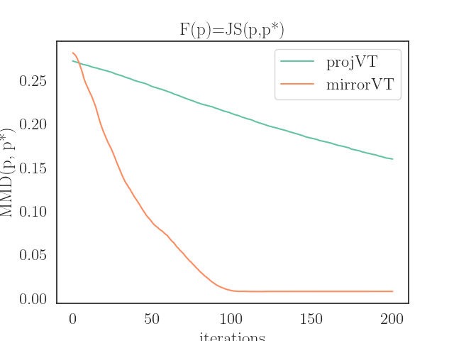
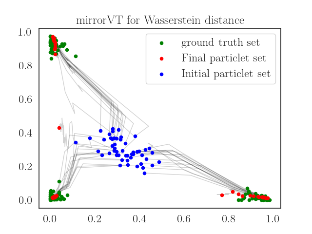
Figure 3: Simulation from two-components Gaussian mixture truncated by the unit ball: trajectories of particles updated by mirrorVT (1st column) and projVT (2nd column), and the comparison of methods in terms of convergence in MMD (3rd column). F𝐹F takes the following forms: KL-divergence (1st row), JS-divergence (2nd row) and Wasserstein distance (3rd row). Green: particles from the target distribution, Blue: initial particle set, Red: the final updated particles.

5.2 Comparing methods

For comparison, we consider the projected variational transport (named projVT) which is a simple variant of VT for the constrained domain. Its update simply has two steps for t𝑡t-th iteration: 1) pushing the particles in the direction of f~tsubscriptsuperscript~𝑓𝑡\tilde{f}^{*}_{t} and 2) projecting back to the constrained domain by the projection operation. In particular, for the unit ball dsuperscript𝑑\mathcal{B}^{d}, the projection operation can be easily computed by: projd(x)=argminydxy2=x/max{1,x2}subscriptprojsuperscript𝑑xsubscriptargminysuperscript𝑑subscriptdelimited-∥∥xy2x1subscriptdelimited-∥∥x2\texttt{proj}_{\mathcal{B}^{d}}(\textbf{x})=\mathop{\rm arg~{}min}\limits_{\textbf{y}\in\mathcal{B}^{d}}\lVert\textbf{x}-\textbf{y}\rVert_{2}=\textbf{x}/\max\left\{1,\lVert\textbf{x}\rVert_{2}\right\}.

For the simplex, the projection operation can be defined as:

projΔd(x)=argminyΔdxy22 subject to i=1dyi=1,yi0i[d]formulae-sequencesubscriptprojsuperscriptΔ𝑑xsubscriptargminysuperscriptΔ𝑑superscriptsubscriptdelimited-∥∥xy22 subject to superscriptsubscript𝑖1𝑑subscripty𝑖1subscripty𝑖0for-all𝑖delimited-[]𝑑\displaystyle\texttt{proj}_{\Delta^{d}}(\textbf{x})=\mathop{\rm arg~{}min}\limits_{\textbf{y}\in\Delta^{d}}\lVert\textbf{x}-\textbf{y}\rVert_{2}^{2}\text{ subject to }\sum_{i=1}^{d}\textbf{y}_{i}=1,\textbf{y}_{i}\geq 0\forall i\in[d]

which can be efficiently solved [4]. For mirrorVT, we need to define the mirror maps. In particular, for the unit ball, a possible map is:

φ(x)=log(1x)x𝜑x1delimited-∥∥xdelimited-∥∥x\displaystyle\varphi(\textbf{x})=-\log(1-\lVert\textbf{x}\rVert)-\lVert\textbf{x}\rVert (28)

and for a simplex, the most natural choice of the map φ𝜑\varphi is the entropic mirror map (see [2]):

φ(x)=i=1d1xilogxi+(1i=1d1xi)log(1i=1d1xi),xΔdformulae-sequence𝜑xsuperscriptsubscript𝑖1𝑑1subscriptx𝑖subscriptx𝑖1superscriptsubscript𝑖1𝑑1subscriptx𝑖1superscriptsubscript𝑖1𝑑1subscriptx𝑖for-allxsuperscriptΔ𝑑\displaystyle\varphi(\textbf{x})=\sum_{i=1}^{d-1}\textbf{x}_{i}\log\textbf{x}_{i}+\left(1-\sum_{i=1}^{d-1}\textbf{x}_{i}\right)\log\left(1-\sum_{i=1}^{d-1}\textbf{x}_{i}\right),\forall\textbf{x}\in\Delta^{d} (29)

The details of φ(x)𝜑x\nabla\varphi(\textbf{x}), φ(x)superscript𝜑x\nabla\varphi^{*}(\textbf{x}) and 2φ(x)1superscript2𝜑superscriptx1\nabla^{2}\varphi(\textbf{x})^{-1} associated with these mirror maps are given in the Appendix A.3.
Refer to caption
Refer to caption
Refer to caption
Refer to caption
Refer to caption
Refer to caption
Refer to caption
Refer to caption
Refer to caption
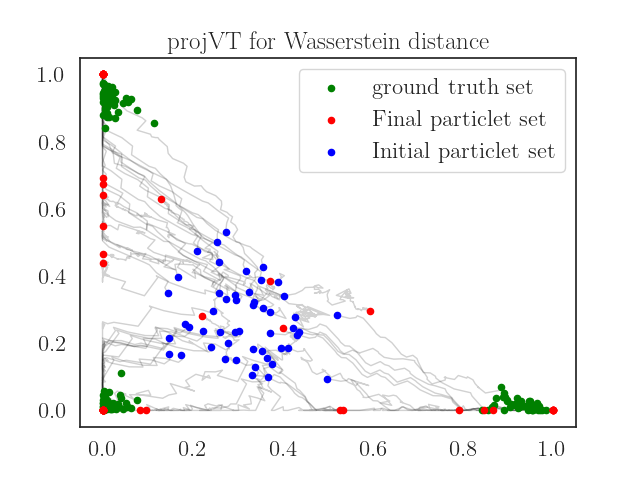
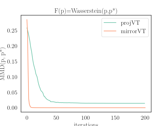
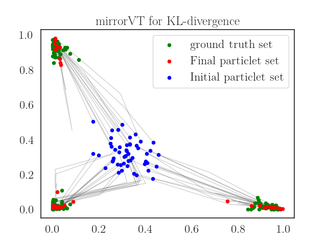
Figure 4: Simulation from three-components Dirichlet mixture: trajectories of particles updated by mirrorVT (1st column) and projVT (2nd column), and the comparison of methods in terms of convergence in MMD (3rd column). F𝐹F takes the following forms: KL-divergence (1st row), JS-divergence (2nd row) and Wasserstein distance (3rd row). Green: particles from the target distribution, Blue: initial particle set, Red: the final updated particles.

5.3 Results

We compare the quality of particles updated by projVT and mirrorVT on the synthetic data samples. The step sizes for projVT and mirrorVT are fine-tuned and set to 0.01 and 0.1, respectively, and we run T=500𝑇500T=500 particle updates. We measure the quality of particle sets by computing their maximum mean discrepancy (MMD, [5]) to the ground truth particle set which represents the target distribution. We stop the particle updates if no improvement in MMD after 20 consecutive updates is observed. Hence we take the following forms of F𝐹F: KL-divergence, JS-divergence and Wasserstein distance.

On the truncated Gaussian mixture sample data, we observe that the particles updated by mirrorVT can well approximate the ground truth samples while those updated by projVT tend to stay in the boundary of the domain (see Fig. 3). This can be explained by the nature of the projection operations. Especially, for the case of JS-divergence, projVT fails to converge to the target distribution. Furthermore, by measuring MMD of particles over iterations, we can find that the convergence of mirrorVT is significant better than that of projVT.

On the simplex sample data, similarly, particles updated by mirrorVT approximate the ground truth samples much better than those updated by projVT (see Fig. 4). Again, particles by projVT mostly stay in the boundary with poorer quality (illustrated by the trajectories of particles and convergence of MMD). In the case of JS-divergence, projVT also fails to approximate the target particle set, while its particles mostly stay in the boundary in the case of Wasserstein distance. The above observations indicate the superior performance of mirrorVT in the distributional optimization problem on the constrained domains.

6 Conclusions And Future Works

In this work, we have considered the distributional optimization problem where probability distributions are defined over the constrained domain. Motivated by the MD algorithm for the constrained optimization, we have presented an iterative particle-based framework, named mirrorVT, to solve the problem in the unconstrained dual space induced by the mirror map. In particular, for each iteration, mirrorVT maps particles to the unconstrained dual space via the mirror map, then approximately performs Wasserstein gradient descent in the dual space by the VT framework [7] and finally maps the updated particles back to the constrained domain. Furthermore, we also analyze theoretical properties of mirrorVT and characterize its convergence to the optimal solution of the objective functional.

However, there are some open questions we would like to address in our future works, for instance, whether it is possible to accelerate the distributional optimization algorithms by applying Nesterov momentum techniques with both of the cases: unconstrained and constrained domains. We also would like to consider the development of distributional optimization algorithms for the functionals which do not admit the variational form.

References

  • Ahn and Chewi [2021] Kwangjun Ahn and Sinho Chewi. Efficient constrained sampling via the mirror-langevin algorithm. Advances in Neural Information Processing Systems, 34:28405–28418, 2021.
  • Beck and Teboulle [2003] Amir Beck and Marc Teboulle. Mirror descent and nonlinear projected subgradient methods for convex optimization. Operations Research Letters, 31(3):167–175, 2003.
  • Cheng and Bartlett [2018] Xiang Cheng and Peter Bartlett. Convergence of langevin mcmc in kl-divergence. In Algorithmic Learning Theory, pages 186–211. PMLR, 2018.
  • Duchi et al. [2008] John Duchi, Shai Shalev-Shwartz, Yoram Singer, and Tushar Chandra. Efficient projections onto the l 1-ball for learning in high dimensions. In Proceedings of the 25th international conference on Machine learning, pages 272–279, 2008.
  • Gretton et al. [2012] Arthur Gretton, Karsten M Borgwardt, Malte J Rasch, Bernhard Schölkopf, and Alexander Smola. A kernel two-sample test. The Journal of Machine Learning Research, 13(1):723–773, 2012.
  • Hsieh et al. [2018] Ya-Ping Hsieh, Ali Kavis, Paul Rolland, and Volkan Cevher. Mirrored langevin dynamics. Advances in Neural Information Processing Systems, 31, 2018.
  • Liu et al. [2021] Lewis Liu, Yufeng Zhang, Zhuoran Yang, Reza Babanezhad, and Zhaoran Wang. Infinite-dimensional optimization for zero-sum games via variational transport. In International Conference on Machine Learning, pages 7033–7044. PMLR, 2021.
  • Liu and Wang [2016] Qiang Liu and Dilin Wang. Stein variational gradient descent: A general purpose bayesian inference algorithm. Advances in neural information processing systems, 29, 2016.
  • Ma et al. [2015] Yi-An Ma, Tianqi Chen, and Emily Fox. A complete recipe for stochastic gradient mcmc. Advances in neural information processing systems, 28, 2015.
  • Rosasco et al. [2009] Lorenzo Rosasco, Mikhail Belkin, and Ernesto De Vito. A note on learning with integral operators. In COLT. Citeseer, 2009.
  • Santambrogio [2017] Filippo Santambrogio. {{\{Euclidean, metric, and Wasserstein}}\} gradient flows: an overview. Bulletin of Mathematical Sciences, 7(1):87–154, 2017.
  • Shi et al. [2021] Jiaxin Shi, Chang Liu, and Lester Mackey. Sampling with mirrored stein operators. arXiv preprint arXiv:2106.12506, 2021.
  • Villani [2009] Cédric Villani. Optimal transport: old and new, volume 338. Springer, 2009.
  • Welling and Teh [2011] Max Welling and Yee W Teh. Bayesian learning via stochastic gradient langevin dynamics. In Proceedings of the 28th international conference on machine learning (ICML-11), pages 681–688, 2011.
  • Wibisono [2018] Andre Wibisono. Sampling as optimization in the space of measures: The langevin dynamics as a composite optimization problem. In Conference on Learning Theory, pages 2093–3027. PMLR, 2018.
  • Xu et al. [2018] Pan Xu, Jinghui Chen, Difan Zou, and Quanquan Gu. Global convergence of langevin dynamics based algorithms for nonconvex optimization. Advances in Neural Information Processing Systems, 31, 2018.
  • Zhang and Sra [2016] Hongyi Zhang and Suvrit Sra. First-order methods for geodesically convex optimization. In Conference on Learning Theory, pages 1617–1638. PMLR, 2016.

Appendix A Appendices

A.1 Proof of Theorem 2

.

Proof.

We have assumed F(p)=KL(p||p)F(p)=\text{KL}(p||p^{*}) for p,p𝒫2(𝒳)𝑝superscript𝑝subscript𝒫2𝒳p,p^{*}\in\mathcal{P}_{2}(\mathcal{X}), so G(q)=KL(q||q)G(q)=\text{KL}(q||q^{*}), for q,q𝒫2(𝒴)𝑞superscript𝑞subscript𝒫2𝒴q,q^{*}\in\mathcal{P}_{2}(\mathcal{Y}). By the definition of the first variation of a functional, we have:

ddϵG(q+ϵχ)|ϵ=0=𝒴Gq(y)χ(y)dy, for all χ𝒫2(𝒴)evaluated-atdditalic-ϵ𝐺𝑞italic-ϵ𝜒italic-ϵ0subscript𝒴𝐺𝑞y𝜒ydifferential-dy, for all 𝜒subscript𝒫2𝒴\displaystyle\frac{\mathrm{d}}{\mathrm{d}\epsilon}G(q+\epsilon\chi)\bigg{|}_{\epsilon=0}=\int_{\mathcal{Y}}\frac{\partial G}{\partial q}(\textbf{y})\chi(\textbf{y})\mathrm{d}\textbf{y}\text{, for all }\chi\in\mathcal{P}_{2}(\mathcal{Y})

We can compute the left-hand side as follows:

ddϵG(q+ϵχ)|ϵ=0evaluated-atdditalic-ϵ𝐺𝑞italic-ϵ𝜒italic-ϵ0\displaystyle\frac{\mathrm{d}}{\mathrm{d}\epsilon}G(q+\epsilon\chi)\bigg{|}_{\epsilon=0} =ddϵKL(q+ϵχ||q)|ϵ=0\displaystyle=\frac{\mathrm{d}}{\mathrm{d}\epsilon}\text{KL}(q+\epsilon\chi||q^{*})\bigg{|}_{\epsilon=0}
=ddϵ(q+ϵχ)log(q+ϵχq)dy|ϵ=0absentevaluated-atdditalic-ϵ𝑞italic-ϵ𝜒𝑞italic-ϵ𝜒superscript𝑞differential-dyitalic-ϵ0\displaystyle=\frac{\mathrm{d}}{\mathrm{d}\epsilon}\int(q+\epsilon\chi)\log\left(\frac{q+\epsilon\chi}{q^{*}}\right)\mathrm{d}\textbf{y}\bigg{|}_{\epsilon=0}
=logqq(y)χ(y)dyabsent𝑞superscript𝑞y𝜒ydifferential-dy\displaystyle=\int\log\frac{q}{q^{*}}(\textbf{y})\chi(\textbf{y})\mathrm{d}\textbf{y}

which indicates that G/q=logqlogq𝐺𝑞𝑞superscript𝑞\partial G/\partial q=\log q-\log q^{*}. For t𝑡t-th iteration, the update direction vtsubscript𝑣𝑡v_{t} is given by:

vt(x)=2φ(x)1ft(x)=gt(y)=logqt(y)logq(y)subscript𝑣𝑡xsuperscript2𝜑superscriptx1subscriptsuperscript𝑓𝑡xsubscriptsuperscript𝑔𝑡ysubscript𝑞𝑡ysuperscript𝑞y\displaystyle\begin{split}v_{t}(\textbf{x})&=\nabla^{2}\varphi(\textbf{x})^{-1}\nabla f^{*}_{t}(\textbf{x})=\nabla g^{*}_{t}(\textbf{y})\\ &=\nabla\log q_{t}(\textbf{y})-\nabla\log q^{*}(\textbf{y})\end{split} (30)

for all x𝒳,y=φ(x)𝒴formulae-sequencex𝒳y𝜑x𝒴\textbf{x}\in\mathcal{X},\textbf{y}=\nabla\varphi(\textbf{x})\in\mathcal{Y}. By applying the integral operator k,ptsubscript𝑘subscript𝑝𝑡\mathcal{L}_{k,p_{t}} (see Definition 1) to vtsubscript𝑣𝑡v_{t}, we obtain:

k,ptvt(x)=𝒳k(x,x)vt(x)pt(x)dx=𝒴kφ(y,y)logqt(y)qt(y)dy𝒴kφ(y,y)logq(y)qt(y)dy=𝒴kφ(y,y)qt(y)dy𝒴kφ(y,y)logq(y)qt(y)dy=𝒴kφ(y,y)qt(y)dy𝒴kφ(y,y)logq(y)qt(y)dy=𝔼yqtkφ(y,y)logq(y)+kφ(y,y)subscript𝑘subscript𝑝𝑡subscript𝑣𝑡xsubscript𝒳𝑘xsuperscriptxsubscript𝑣𝑡superscriptxsubscript𝑝𝑡superscriptxdifferential-dsuperscriptxsubscript𝒴subscript𝑘𝜑ysuperscriptysubscript𝑞𝑡superscriptysubscript𝑞𝑡superscriptydifferential-dsuperscriptysubscript𝒴subscript𝑘𝜑ysuperscriptysuperscript𝑞superscriptysubscript𝑞𝑡superscriptydifferential-dsuperscriptysubscript𝒴subscript𝑘𝜑ysuperscriptysubscript𝑞𝑡superscriptydifferential-dsuperscriptysubscript𝒴subscript𝑘𝜑ysuperscriptysuperscript𝑞superscriptysubscript𝑞𝑡superscriptydifferential-dsuperscriptysubscript𝒴subscript𝑘𝜑ysuperscriptysubscript𝑞𝑡superscriptydifferential-dsuperscriptysubscript𝒴subscript𝑘𝜑ysuperscriptysuperscript𝑞superscriptysubscript𝑞𝑡superscriptydifferential-dsuperscriptysubscript𝔼similar-tosuperscriptysubscript𝑞𝑡subscript𝑘𝜑ysuperscriptysuperscript𝑞superscriptysubscript𝑘𝜑ysuperscripty\displaystyle\begin{split}\mathcal{L}_{k,p_{t}}v_{t}(\textbf{x})&=\int_{\mathcal{X}}k(\textbf{x},\textbf{x}^{\prime})v_{t}(\textbf{x}^{\prime})p_{t}(\textbf{x}^{\prime})\mathrm{d}\textbf{x}^{\prime}\\ &=\int_{\mathcal{Y}}k_{\varphi}(\textbf{y},\textbf{y}^{\prime})\nabla\log q_{t}(\textbf{y}^{\prime})q_{t}(\textbf{y}^{\prime})\mathrm{d}\textbf{y}^{\prime}-\int_{\mathcal{Y}}k_{\varphi}(\textbf{y},\textbf{y}^{\prime})\nabla\log q^{*}(\textbf{y}^{\prime})q_{t}(\textbf{y}^{\prime})\mathrm{d}\textbf{y}^{\prime}\\ &=\int_{\mathcal{Y}}k_{\varphi}(\textbf{y},\textbf{y}^{\prime})\nabla q_{t}(\textbf{y}^{\prime})\mathrm{d}\textbf{y}^{\prime}-\int_{\mathcal{Y}}k_{\varphi}(\textbf{y},\textbf{y}^{\prime})\nabla\log q^{*}(\textbf{y}^{\prime})q_{t}(\textbf{y}^{\prime})\mathrm{d}\textbf{y}^{\prime}\\ &=-\int_{\mathcal{Y}}\nabla k_{\varphi}(\textbf{y},\textbf{y}^{\prime})q_{t}(\textbf{y}^{\prime})\mathrm{d}\textbf{y}^{\prime}-\int_{\mathcal{Y}}k_{\varphi}(\textbf{y},\textbf{y}^{\prime})\nabla\log q^{*}(\textbf{y}^{\prime})q_{t}(\textbf{y}^{\prime})\mathrm{d}\textbf{y}^{\prime}\\ &=-\mathbb{E}_{\textbf{y}^{\prime}\sim q_{t}}k_{\varphi}(\textbf{y},\textbf{y}^{\prime})\nabla\log q^{*}(\textbf{y}^{\prime})+\nabla k_{\varphi}(\textbf{y},\textbf{y}^{\prime})\end{split} (31)

The first equality is obtained by the definition of the integral operator (see Definition 1), the second equality is obtained by using (30) and the forth equality is obtained by applying the integration by parts to the first term. The proof is completed. ∎

A.2 Proof of Theorem 3

Proof.

We analyze the performance of one step of mirrorVT. Under the Assumption 1.1 (L2subscript𝐿2L_{2}-smoothness of G𝐺G), for any t0𝑡0t\geq 0, we have:

G(qt+1)G(qt)+gradG(qt),Expqt1(qt+1)qt+1/2L2𝒲22(qt+1,qt)=G(qt)ηtgradG(qt),gradG(qt)+δ~tqt+1/2L2ηt2gradG(qt)+δ~t,gradG(qt)+δ~tqt=G(qt)ηtgradG(qt),gradG(qt)qtηtgradG(qt),δ~tqt+1/2L2ηt2gradG(qt)+δ~t,gradG(qt)+δ~tqt𝐺subscript𝑞𝑡1𝐺subscript𝑞𝑡subscriptgrad𝐺subscript𝑞𝑡superscriptsubscriptExpsubscript𝑞𝑡1subscript𝑞𝑡1subscript𝑞𝑡12subscript𝐿2subscriptsuperscript𝒲22subscript𝑞𝑡1subscript𝑞𝑡𝐺subscript𝑞𝑡subscript𝜂𝑡subscriptgrad𝐺subscript𝑞𝑡grad𝐺subscript𝑞𝑡subscript~𝛿𝑡subscript𝑞𝑡12subscript𝐿2superscriptsubscript𝜂𝑡2subscriptgrad𝐺subscript𝑞𝑡subscript~𝛿𝑡grad𝐺subscript𝑞𝑡subscript~𝛿𝑡subscript𝑞𝑡𝐺subscript𝑞𝑡subscript𝜂𝑡subscriptgrad𝐺subscript𝑞𝑡grad𝐺subscript𝑞𝑡subscript𝑞𝑡subscript𝜂𝑡subscriptgrad𝐺subscript𝑞𝑡subscript~𝛿𝑡subscript𝑞𝑡12subscript𝐿2superscriptsubscript𝜂𝑡2subscriptgrad𝐺subscript𝑞𝑡subscript~𝛿𝑡grad𝐺subscript𝑞𝑡subscript~𝛿𝑡subscript𝑞𝑡\displaystyle\begin{split}G(q_{t+1})&\leq G(q_{t})+\langle\texttt{grad}G(q_{t}),\texttt{Exp}_{q_{t}}^{-1}(q_{t+1})\rangle_{q_{t}}+1/2L_{2}\cdot\mathcal{W}^{2}_{2}(q_{t+1},q_{t})\\ &=G(q_{t})-\eta_{t}\langle\texttt{grad}G(q_{t}),\texttt{grad}G(q_{t})+\tilde{\delta}_{t}\rangle_{q_{t}}+1/2L_{2}\eta_{t}^{2}\langle\texttt{grad}G(q_{t})+\tilde{\delta}_{t},\texttt{grad}G(q_{t})+\tilde{\delta}_{t}\rangle_{q_{t}}\\ &=G(q_{t})-\eta_{t}\langle\texttt{grad}G(q_{t}),\texttt{grad}G(q_{t})\rangle_{q_{t}}-\eta_{t}\langle\texttt{grad}G(q_{t}),\tilde{\delta}_{t}\rangle_{q_{t}}\\ &+1/2L_{2}\eta_{t}^{2}\langle\texttt{grad}G(q_{t})+\tilde{\delta}_{t},\texttt{grad}G(q_{t})+\tilde{\delta}_{t}\rangle_{q_{t}}\end{split} (32)

where ηt(0,α/h]subscript𝜂𝑡0𝛼\eta_{t}\in\left(0,\alpha/h\right] (see (11)) and δ~t=div(qt(gt~gt))subscript~𝛿𝑡divsubscript𝑞𝑡~superscriptsubscript𝑔𝑡subscriptsuperscript𝑔𝑡\tilde{\delta}_{t}=-\texttt{div}(q_{t}(\nabla\tilde{g_{t}^{*}}-\nabla g^{*}_{t})) is the difference between the true 222-Wasserstein gradient at qtsubscript𝑞𝑡q_{t} given by gradG(qt)=div(qtgt)grad𝐺subscript𝑞𝑡divsubscript𝑞𝑡subscriptsuperscript𝑔𝑡\texttt{grad}G(q_{t})=-\texttt{div}(q_{t}\nabla g^{*}_{t}) and its estimate given by div(qtgt~)divsubscript𝑞𝑡~superscriptsubscript𝑔𝑡-\texttt{div}(q_{t}\nabla\tilde{g_{t}^{*}}). The corresponding expected gradient error for G𝐺G is defined as:

ϵ~t=𝔼δ~t,δ~tqt=𝔼2φ(x)1(ft~(x)ft(x))22pt(x)dxsubscript~italic-ϵ𝑡𝔼subscriptsubscript~𝛿𝑡subscript~𝛿𝑡subscript𝑞𝑡𝔼subscriptsuperscriptdelimited-∥∥superscript2𝜑superscriptx1~superscriptsubscript𝑓𝑡xsubscriptsuperscript𝑓𝑡x22subscript𝑝𝑡xdifferential-dx\displaystyle\tilde{\epsilon}_{t}=\mathbb{E}\langle\tilde{\delta}_{t},\tilde{\delta}_{t}\rangle_{q_{t}}=\mathbb{E}\int\lVert\nabla^{2}\varphi(\textbf{x})^{-1}\left(\nabla\tilde{f_{t}^{*}}(\textbf{x})-\nabla f^{*}_{t}(\textbf{x})\right)\rVert^{2}_{2}p_{t}(\textbf{x})\mathrm{d}\textbf{x} (33)

Also since 0αI2φ(x)precedes0𝛼Iprecedes-or-equalssuperscript2𝜑x0\prec\alpha\textbf{I}\preceq\nabla^{2}\varphi(\textbf{x}) for all x𝒳x𝒳\textbf{x}\in\mathcal{X}, we have

ϵ~t1α2ϵtsubscript~italic-ϵ𝑡1superscript𝛼2subscriptitalic-ϵ𝑡\displaystyle\tilde{\epsilon}_{t}\leq\frac{1}{\alpha^{2}}\epsilon_{t} (34)

By applying the basic inequality: gradG(qt),δ~t12gradG(qt),gradG(qt)+12δ~t,δ~tgrad𝐺subscript𝑞𝑡subscript~𝛿𝑡12grad𝐺subscript𝑞𝑡grad𝐺subscript𝑞𝑡12subscript~𝛿𝑡subscript~𝛿𝑡\langle\texttt{grad}G(q_{t}),\tilde{\delta}_{t}\rangle\leq\frac{1}{2}\langle\texttt{grad}G(q_{t}),\texttt{grad}G(q_{t})\rangle+\frac{1}{2}\langle\tilde{\delta}_{t},\tilde{\delta}_{t}\rangle and combining with (34), we have:

G(qt+1)G(qt)1/2ηt(12ηtL2)gradG(qt),gradG(qt)qt+ηt(1+2ηtL2)2α2ϵt𝐺subscript𝑞𝑡1𝐺subscript𝑞𝑡12subscript𝜂𝑡12subscript𝜂𝑡subscript𝐿2subscriptgrad𝐺subscript𝑞𝑡grad𝐺subscript𝑞𝑡subscript𝑞𝑡subscript𝜂𝑡12subscript𝜂𝑡subscript𝐿22superscript𝛼2subscriptitalic-ϵ𝑡\displaystyle\begin{split}G(q_{t+1})&\leq G(q_{t})-1/2\cdot\eta_{t}(1-2\eta_{t}L_{2})\cdot\langle\texttt{grad}G(q_{t}),\texttt{grad}G(q_{t})\rangle_{q_{t}}+\frac{\eta_{t}(1+2\eta_{t}L_{2})}{2\alpha^{2}}\epsilon_{t}\\ \end{split} (35)

By the definition of the inner product on the tangent space and the assumption of μ𝜇\mu-strong convexity of F𝐹F, we obtain the following inequality:

gradG(qt),gradG(qt)qt=𝒴gt(y)22qt(y)dy=𝒳2φ(x)ft(x)22pt(x)dx1α2𝒳ft(x)22pt(x)dx=1α2gradF(pt),gradF(pt)ptμα2(F(pt)F(p))subscriptgrad𝐺subscript𝑞𝑡grad𝐺subscript𝑞𝑡subscript𝑞𝑡subscript𝒴superscriptsubscriptdelimited-∥∥subscriptsuperscript𝑔𝑡y22subscript𝑞𝑡ydifferential-dysubscript𝒳superscriptsubscriptdelimited-∥∥superscript2𝜑xsubscriptsuperscript𝑓𝑡x22subscript𝑝𝑡xdifferential-dx1superscript𝛼2subscript𝒳superscriptsubscriptdelimited-∥∥subscriptsuperscript𝑓𝑡x22subscript𝑝𝑡xdifferential-dx1superscript𝛼2subscriptgrad𝐹subscript𝑝𝑡grad𝐹subscript𝑝𝑡subscript𝑝𝑡𝜇superscript𝛼2𝐹subscript𝑝𝑡𝐹superscript𝑝\displaystyle\begin{split}\langle\texttt{grad}G(q_{t}),\texttt{grad}G(q_{t})\rangle_{q_{t}}&=\int_{\mathcal{Y}}\lVert\nabla g^{*}_{t}(\textbf{y})\rVert_{2}^{2}q_{t}(\textbf{y})\mathrm{d}\textbf{y}\\ &=\int_{\mathcal{X}}\lVert\nabla^{2}\varphi(\textbf{x})\nabla f^{*}_{t}(\textbf{x})\rVert_{2}^{2}p_{t}(\textbf{x})\mathrm{d}\textbf{x}\\ &\geq\frac{1}{\alpha^{2}}\int_{\mathcal{X}}\lVert\nabla f^{*}_{t}(\textbf{x})\rVert_{2}^{2}p_{t}(\textbf{x})\mathrm{d}\textbf{x}=\frac{1}{\alpha^{2}}\langle\texttt{grad}F(p_{t}),\texttt{grad}F(p_{t})\rangle_{p_{t}}\\ &\geq\frac{\mu}{\alpha^{2}}\left(F(p_{t})-F(p^{*})\right)\end{split} (36)

where the first inequality is obtained by 2φ(x)βIprecedes-or-equalssuperscript2𝜑x𝛽I\nabla^{2}\varphi(\textbf{x})\preceq\beta\textbf{I} for all x𝒳x𝒳\textbf{x}\in\mathcal{X} and the second inequality is obtained by Assumption 1.3 (see (26)). Thus combining (35) and use the identity: F(pt)=G(qt)𝐹subscript𝑝𝑡𝐺subscript𝑞𝑡F(p_{t})=G(q_{t}), we have:

F(pt+1)F(pt)[1μηt2β2(12ηtL2))](F(pt)F)+ηt(1+2ηtL2)2α2ϵt\displaystyle F(p_{t+1})-F(p_{t})\leq\left[1-\frac{\mu\eta_{t}}{2\beta^{2}}(1-2\eta_{t}L_{2}))\right]\left(F(p_{t})-F^{*}\right)+\frac{\eta_{t}(1+2\eta_{t}L_{2})}{2\alpha^{2}}\epsilon_{t} (37)

By setting ηt=ηmin{12L2,1μβ2}subscript𝜂𝑡𝜂12subscript𝐿21𝜇superscript𝛽2\eta_{t}=\eta\leq\min\left\{\frac{1}{2L_{2}},\frac{1}{\mu\beta^{2}}\right\}, we have:

1μηt2β2(12ηtL2))1μηt2β2,01μη2β2 and η(1+2ηL2)2α2ηα2\displaystyle 1-\frac{\mu\eta_{t}}{2\beta^{2}}\left(1-2\eta_{t}L_{2})\right)\leq 1-\frac{\mu\eta_{t}}{2\beta^{2}},0\leq 1-\frac{\mu\eta}{2\beta^{2}}\text{ and }\frac{\eta(1+2\eta L_{2})}{2\alpha^{2}}\leq\frac{\eta}{\alpha^{2}} (38)

In the sequel, we define ρ=1μη2β2[0,1]𝜌1𝜇𝜂2superscript𝛽201\rho=1-\frac{\mu\eta}{2\beta^{2}}\in\left[0,1\right], we have:

F(pt+1)F(pt)ρ(F(pt)F)+ηtα2ϵt𝐹subscript𝑝𝑡1𝐹subscript𝑝𝑡𝜌𝐹subscript𝑝𝑡superscript𝐹subscript𝜂𝑡superscript𝛼2subscriptitalic-ϵ𝑡\displaystyle F(p_{t+1})-F(p_{t})\leq\rho\left(F(p_{t})-F^{*}\right)+\frac{\eta_{t}}{\alpha^{2}}\epsilon_{t} (39)

By forming a telescoping sequence and combining the upper bound of ϵtsubscriptitalic-ϵ𝑡\epsilon_{t} given in [7], we have:

F(pt+1)infp𝒫2(𝒳)F(p)ρt(F(p1)infp𝒫2(𝒳)F(p))+1ρt1ρηα2Error𝐹subscript𝑝𝑡1subscriptinfimum𝑝subscript𝒫2𝒳𝐹𝑝superscript𝜌𝑡𝐹subscript𝑝1subscriptinfimum𝑝subscript𝒫2𝒳𝐹𝑝1superscript𝜌𝑡1𝜌𝜂superscript𝛼2Error\displaystyle F(p_{t+1})-\inf_{p\in\mathcal{P}_{2}(\mathcal{X})}F(p)\leq\rho^{t}\left(F(p_{1})-\inf_{p\in\mathcal{P}_{2}(\mathcal{X})}F(p)\right)+\frac{1-\rho^{t}}{1-\rho}\frac{\eta}{\alpha^{2}}\cdot\texttt{Error} (40)

Finally, by taking the expectation over the initial particle set, we complete the proof. ∎

A.3 Details Of The Mirror Maps

In this section, we describe more details of the mirror maps used in our simulated experiments.

A.3.1 Mirror Map On The Unit Ball

For the mirror map defined in (28), we can easily shown that:

φxi=xi1x2,φyi=yi1+y2,2φxixj=δij1x2+xixjx2(1x2)2formulae-sequence𝜑subscriptx𝑖subscriptx𝑖1subscriptdelimited-∥∥x2formulae-sequencesuperscript𝜑subscripty𝑖subscripty𝑖1subscriptdelimited-∥∥y2superscript2𝜑subscriptx𝑖subscriptx𝑗subscript𝛿𝑖𝑗1subscriptdelimited-∥∥x2subscriptx𝑖subscriptx𝑗subscriptdelimited-∥∥x2superscript1subscriptdelimited-∥∥x22\frac{\partial\varphi}{\partial\textbf{x}_{i}}=\frac{\textbf{x}_{i}}{1-\lVert\textbf{x}\rVert_{2}},\frac{\partial\varphi^{*}}{\partial\textbf{y}_{i}}=\frac{\textbf{y}_{i}}{1+\lVert\textbf{y}\rVert_{2}},\frac{\partial^{2}\varphi}{\partial\textbf{x}_{i}\partial\textbf{x}_{j}}=\frac{\delta_{ij}}{1-\lVert\textbf{x}\rVert_{2}}+\frac{\textbf{x}_{i}\textbf{x}_{j}}{\lVert\textbf{x}\rVert_{2}\left(1-\lVert\textbf{x}\rVert_{2}\right)^{2}}

Hence the Hessian matrix can be written as: 2φ(x)=11x2I+1x2(1x2)2xxsuperscript2𝜑x11subscriptdelimited-∥∥x2I1subscriptdelimited-∥∥x2superscript1subscriptdelimited-∥∥x22superscriptxxtop\nabla^{2}\varphi(\textbf{x})=\frac{1}{1-\lVert\textbf{x}\rVert_{2}}\textbf{I}+\frac{1}{\lVert\textbf{x}\rVert_{2}\left(1-\lVert\textbf{x}\rVert_{2}\right)^{2}}\textbf{x}\textbf{x}^{\top}, where I is the identity matrix. In order to obtain the inversion of Hessian matrix, we apply the celebrated Woodbury matrix identity and show that

(2φ(x))1=(1x2)(I1x2xx)superscriptsuperscript2𝜑x11subscriptdelimited-∥∥x2I1subscriptdelimited-∥∥x2superscriptxxtop\left(\nabla^{2}\varphi(\textbf{x})\right)^{-1}=\left(1-\lVert\textbf{x}\rVert_{2}\right)\left(\textbf{I}-\frac{1}{\lVert\textbf{x}\rVert_{2}}\textbf{x}\textbf{x}^{\top}\right)

A.3.2 Mirror Map On The Simplex

For the entropic mirror map (see [2]), we can consider x=[x1,,xd1]d1xsubscriptx1subscriptx𝑑1superscript𝑑1\textbf{x}=\left[\textbf{x}_{1},...,\textbf{x}_{d-1}\right]\in\mathbb{R}^{d-1} by discarding the last entry xd=1i=1d1xisubscriptx𝑑1superscriptsubscript𝑖1𝑑1subscriptx𝑖\textbf{x}_{d}=1-\sum_{i=1}^{d-1}\textbf{x}_{i} and easily show that:

φxi=logxilogxd,φyi=exp(yi)j=1d1exp(yj),2φxixj=δijxi+1xd,i[d1]formulae-sequence𝜑subscriptx𝑖subscriptx𝑖subscriptx𝑑formulae-sequencesuperscript𝜑subscripty𝑖subscripty𝑖superscriptsubscript𝑗1𝑑1subscripty𝑗formulae-sequencesuperscript2𝜑subscriptx𝑖subscriptx𝑗subscript𝛿𝑖𝑗subscriptx𝑖1subscriptx𝑑for-all𝑖delimited-[]𝑑1\frac{\partial\varphi}{\partial\textbf{x}_{i}}=\log\textbf{x}_{i}-\log\textbf{x}_{d},\frac{\partial\varphi^{*}}{\partial\textbf{y}_{i}}=\frac{\exp{\left(\textbf{y}_{i}\right)}}{\sum_{j=1}^{d-1}\exp{\left(\textbf{y}_{j}\right)}},\frac{\partial^{2}\varphi}{\partial\textbf{x}_{i}\partial\textbf{x}_{j}}=\frac{\delta_{ij}}{\textbf{x}_{i}}+\frac{1}{\textbf{x}_{d}},\forall i\in\left[d-1\right]

Hence the Hessian matrix can be written as: 2φ(x)=diag(1/x1,1/x2,,1/xd1)+1/xd11superscript2𝜑xdiag1subscriptx11subscriptx21subscriptx𝑑11subscriptx𝑑superscript11top\nabla^{2}\varphi(\textbf{x})=\texttt{diag}(1/\textbf{x}_{1},1/\textbf{x}_{2},...,1/\textbf{x}_{d-1})+1/\textbf{x}_{d}\textbf{1}\textbf{1}^{\top}. By applying the Sherman–Morrison formula, we obtain the inverse Hessian matrix of the following form:

(2φ(x))1=diag(x)xxsuperscriptsuperscript2𝜑x1diagxsuperscriptxxtop\left(\nabla^{2}\varphi(\textbf{x})\right)^{-1}=\texttt{diag}(\textbf{x})-\textbf{x}\textbf{x}^{\top}