The Uchuu-SDSS galaxy lightcones: a clustering, RSD and BAO study

Abstract

We present the data release of the Uchuu-SDSS galaxies: a set of 32 high-fidelity galaxy lightcones constructed from the large Uchuu 2.1 trillion particle $N$-body simulation using Planck cosmology. We adopt subhalo abundance matching to populate the Uchuu-box halo catalogues with SDSS galaxy luminosities. These cubic box galaxy catalogues generated at several redshifts are combined to create the set of lightcones with redshift-evolving galaxy properties. The Uchuu-SDSS galaxy lightcones are built to reproduce the footprint and statistical properties of the SDSS main galaxy survey, along with stellar masses and star formation rates. This facilitates direct comparison of the observed SDSS and simulated Uchuu-SDSS data. Our lightcones reproduce a large number of observational results, such as the distribution of galaxy properties, the galaxy clustering, the stellar mass functions, and the halo occupation distributions. Using the simulated and real data we select samples of bright red galaxies at $z_{\mathrm{eff}}=0.15$ to explore Redshift Space Distortions and Baryon Acoustic Oscillations (BAO) utilizing a full-shape analytical model of the two-point correlation function. We create a set of 5100 galaxy lightcones using GLAM N-body simulations to compute covariance errors. We report a $\sim 30\%$ precision increase on $f\sigma_{8}$, due to our better estimate of the covariance matrix. From our BAO-inferred $\alpha_{\parallel}$ and $\alpha_{\perp}$ parameters, we obtain the first SDSS measurements of the Hubble and angular diameter distances $D_{\mathrm{H}}(z=0.15)/r_{d}=27.9^{+3.1}_{-2.7}$, $D_{\mathrm{M}}(z=0.15)/r_{d}=5.1^{+0.4}_{-0.4}$. Overall, we conclude that the Planck CDM cosmology nicely explains the observed large-scale structure statistics of SDSS. All data sets are made publicly available.

1 Introduction

Galaxy redshift surveys, measuring the spatial distribution of galaxies throughout cosmic time, have proven to be key observational probes for constraining cosmological models and astrophysical phenomena. For example, the distribution of galaxies on large scales can be used to infer cosmological parameters (e.g. Alam et al., 2021), as well as to constrain the properties of dark energy that drives the accelerated expansion of the Universe (Riess et al., 1998; Perlmutter et al., 1999). On smaller scales, the galaxy clustering signal encodes information on how galaxies populate dark matter haloes, on star formation, feedback and other baryonic processes that shape galaxy formation (see Wechsler & Tinker, 2018, for a review).

In order to connect galaxy redshift surveys to theoretical predictions, it is essential to generate high-fidelity galaxy catalogues from cosmological simulations that capture the expected properties and clustering of the observed galaxy sample (e.g. de la Torre et al., 2013; White et al., 2014; Rodríguez-Torres et al., 2016; Lin et al., 2020). Hence, they can be used to increase the amount of information that can be extracted from galaxy survey data. Firstly, the cosmological parameters of the simulation are known exactly. This allows us to assess the systematic and statistical errors of cosmological measurements from galaxy surveys, to compute the covariance errors, to test the performance of statistical analyses, and to aid the theoretical interpretation of survey results. Secondly, high-fidelity catalogues based on simulations allow us to assess the systematics arising from such observational effects as selection function and fibre collisions. These effects are a source for incompleteness in the survey sample. They must to be understood in order to minimise their impact in the measured clustering signal (see Smith et al., 2019, and references therein).

In the last two decades, vast observational efforts such as the 2dF Galaxy Redshift Survey (2dFGRS) (Colless et al., 2001) and the Sloan Digital Sky Survey (SDSS) saga (Alam et al., 2021), have driven most of the major discoveries about the Large-Scale Structure (LSS) of our Universe. The relevance of the SDSS surveys is not purely historical – to date, SDSS continues to be the largest reference galaxy database, offering sky positions, redshifts, spectra and images for millions of galaxies. New technological advances continue to push the depth and volume of galaxy surveys – the new generation of galaxy surveys, which include the Dark Energy Spectroscopic Instrument (DESI) survey (DESI Collaboration et al., 2016), the Large Synoptic Survey Telescope (LSST) (Ivezić et al., 2019), the Subaru Prime Focus Spectrograph (PFS) (Takada et al., 2014) and the Euclid survey (Laureijs et al., 2011), aim to produce unprecedentedly large data sets in an effort to map the Universe to even higher precision.

In order to generate high-fidelity simulated galaxy lightcones for these large surveys, cosmological simulations with high-resolution in a large volume are needed. Although it would be desirable to create mocks from hydrodynamical simulations, in which the formation of galaxies is modelled self-consistently by solving the coupled evolution of both baryons and dark matter (DM), such simulations are complex and computationally expensive. The largest to date do not exceed a few hundred Mpc in box size (e.g. Dubois et al., 2014; Schaye et al., 2015; Pillepich et al., 2018; Springel et al., 2018). Hydrodynamical simulations are also strongly affected by the modelling uncertainties of complex baryonic processes. Thus, one usually resorts to DM-only simulations. Since galaxy formation physics is not included, dark matter halos must be populated with galaxies in order to produce the desired simulated galaxy catalogue. This can be done using a variety of methods, each comprising different assumptions about the galaxy–halo connection (Wechsler & Tinker, 2018).

A common option to generate galaxies from DM halos is to use empirically based methods, such as subhalo abundance matching (SHAM; e.g. Marinoni & Hudson, 2002; Vale & Ostriker, 2004; Kravtsov et al., 2004; Conroy et al., 2006; Rodríguez-Torres et al., 2016; Safonova et al., 2021). In its simplest form, the main underlying assumption is that every halo and subhalo contains a galaxy, and that there are correlations between halo and galaxy properties. For instance, the most massive and luminous galaxies are generally assumed to reside in the most massive haloes. At face value, one can assign galaxies to haloes by generating a rank-ordered relation between observed galaxy luminosities and simulated halo masses. However, such a one-to-one relation between galaxies and halos is incompatible with observations (e.g. Trujillo-Gomez et al., 2011; Shu et al., 2012) – an intrinsic scatter must be incorporated in the method to produce realistic catalogues. Furthermore, the clustering of haloes is observed to depend on properties other than halo mass, including the halo formation time, concentration and spin (e.g. Wechsler, 2001; Gao et al., 2005; Wechsler et al., 2006). Empirical models such as SHAM or the popular HOD method (e.g. Zehavi et al., 2011) are computationally fast, and are able to workaround the uncertainties in the physics of galaxy formation by constraining the model parameters directly with data. Applications of the SHAM method are able to reproduce observed properties of galaxies in large surveys as the luminosity and stellar mass functions or the luminosity and colour-dependent clustering to high accuracy (e.g. Trujillo-Gomez et al., 2011; Rodríguez-Torres et al., 2016).

From real and simulated survey data, the nature of dark energy can be probed for instance by measuring the growth rate of structure, defined in linear theory as $f(a)=d\mathrm{ln}D(a)/d\mathrm{ln}a$, where $a$ is the scale factor and $D(a)$ is the linear growth function. This parameter can be regarded as a measure of the energy content of the Universe, allowing us to constrain different theories of gravity and dark energy (see e.g. Peebles, 1980; Guzzo et al., 2008, for a review). Galaxy peculiar velocities introduce anisotropies in their observed redshifts. This effect, first described in Kaiser (1987), is known as Redshift Space Distortions (RSD). Measurements of RSD in galaxy surveys yield $f\sigma_{8}$, where $\sigma_{8}(z)$ is the normalization of the power spectrum at redshift $z$ on a scale of $8~{}h^{-1}\mathrm{Mpc}$. Another source of anisotropy comes from the choice of the fiducial cosmology adopted in the clustering analysis, used for converting redshifts and angles to comoving coordinates. If the fiducial cosmology differs from the observed one, galaxy clusters will appear flattened or elongated. The study of this so-called Alcock-Paczynski effect can provide an additional source of cosmological information from the data, as well as a means to validate a cosmological model from a simulated galaxy survey.

In addition to RSD, one can measure the Baryon Acoustic Oscillation (BAO) feature from the two-point clustering statistics in galaxy surveys. This allows us to determine the expansion rate of the Universe (e.g. Eisenstein et al., 2005; Cole et al., 2005). Recently, Alam et al. (2021) reported cosmological implications from two decades of SDSS spectroscopic surveys based on clustering measurements from galaxies and quasars in the redshift range $0.1<z<3$. This includes the SDSS DR7 main galaxy sample (MGS), at low redshift $z\sim 0.1$, which clustering statistics is compared in this work with the high-fidelity simulated galaxy light-cones built from on our 2.1 trillion $N$-body Uchuu simulation (Ishiyama et al., 2021).

Our Uchuu-SDSS light-cones are built using the SHAM method to reproduce the basic properties of the SDSS galaxy population, match its sky footprint and selection function, and include the effect of fibre collisions, which facilitates their straightforward comparison with the SDSS MGS data. Furthermore we study and measure RSD and BAO in the real and simulated data to test the Planck base $\Lambda$CDM cosmology model (Planck Collaboration et al., 2020). The Uchuu-SDSS galaxy catalogues include sky positions, redshifts, $ugriz$ apparent and absolute magnitudes stellar masses and star formation rates (SFR), as well as several halo properties. The catalogues are made publicly available at the Skies & Universes website.

The structure of this paper is as follows. In Section 2, we introduce the SDSS MGS data and define the volume-limited galaxy samples used to validate our simulated galaxy catalogues. In Section 3, we describe the Uchuu simulation and the methodology behind the creation of galaxies from the dark matter halo properties. This includes the construction of light-cones from cubic boxes, the implementation of fibre collisions, and the assignment of additional SDSS galaxy properties. Section 4 presents the basic properties of the Uchuu-SDSS light-cones, compared to the SDSS data. In particular, we explore the statistics of several galaxy properties, the galaxy clustering dependence on luminosity, color, and stellar mass, and the galaxy HOD. In Section 5, we present our RSD and BAO measurements both in the real and simulated data, and compare them with the fiducial Planck cosmology. Finally, in Section 6, we present a summary of our results.

2 SDSS Galaxy Samples

2.1 Parent and volume-limited samples

${}^{0.1}M_{r}^{\mathrm{max}}$	$z_{\mathrm{max}}$	$N$	$n_{g}$	$V_{\mathrm{eff}}$	$f_{\mathrm{NN}}$
-18.0	0.041	35359	31.95	1.11	0.043
-18.5	0.053	49272	20.41	2.54	0.046
-19.0	0.064	62534	14.47	4.55	0.050
-19.5	0.085	112652	11.09	10.68	0.058
-20.0	0.106	119734	6.13	20.53	0.062
-20.5	0.132	112496	3.03	39.03	0.068
-21.0	0.159	71795	1.13	66.95	0.079
-21.5	0.198	33505	0.28	125.63	0.099
-22.0	0.245	9820	0.045	218.32	0.149

Table 1: For each SDSS volume-limited sample, the columns list (from left to right): the absolute magnitude threshold, the maximum redshift, the number of galaxies, the galaxy number density (in $10^{-3}~{}h^{3}\mathrm{Mpc}^{-3}$), the effective volume of each sample (in $10^{6}~{}h^{-3}\mathrm{Mpc}^{3}$), and the fraction of galaxies requiring the nearest neighbour correction. The lower redshift cut for all samples is $z_{\mathrm{min}}=0.02$. Magnitudes of all galaxies are $k$–corrected and passively evolved to the survey’s median redshift of $z=0.1$ and computed assuming $h=1$.

In this work, we build and compare Uchuu simulated galaxies to observational data from the seventh data release (DR7; Abazajian et al., 2009) of the SDSS (York et al., 2000). More specifically, we make use of the large scale structure catalog of the SDSS MGS from the NYU Value Added Galaxy Catalogue (NYU-VAGC; Blanton et al., 2005). We restrict our sample to consist only of galaxies in the contiguous northern footprint in regions which have a completeness of $>90\%$. This parent sample covers an effective area of $\sim 6511\ \mathrm{deg}^{2}$ and contains $\sim 497\,000$ galaxies with Petrosian $r$-band magnitudes in the range $14.5<r_{\mathrm{pet}}<17.6$. In this sample, $\sim 6\%$ of targeted galaxies lack a spectroscopically measured redshift due to fibre collisions. We apply a nearest neighbour correction to these galaxies, assigning to them the redshift of the galaxy with which they collided.

Apparent magnitudes can be linked to absolute magnitudes via the distance modulus equation,

$$r={}^{0.1}M_{r}^{h}+5\log_{10}D_{L}(z)+25+{}^{0.1}k_{r}(z),$$ (1)

where $D_{L}(z)$ is the luminosity distance (in units of $h^{-1}\mathrm{Mpc}$), ${}^{0.1}k_{r}(z)$ is the $k$-correction, which takes into account the shift in the bandpass with redshift.

Throughout this paper, we denote $k$-corrected unevolved absolute magnitudes in the $r$-band as ${}^{0.1}M_{r}^{h}\equiv{}^{0.1}M_{r}-5\log_{10}h$, where the superscript 0.1 indicates that the rest-frame magnitude has been $k$-corrected to a reference redshift of $z_{\mathrm{ref}}=0.1$ (Blanton et al., 2003a). A similar notation is used for magnitudes in other bands. We also denote the rest-frame $g-r$ colours as ${}^{0.1}(g-r)$, $k$-corrected to the same reference redshift.

Additionally, the absolute magnitudes are corrected for passive evolution using the model of Blanton (2006). Specifically, the ‘evolved’ magnitude ${}^{0.1}M_{r}^{h,e}$ is given by

$${}^{0.1}M_{r}^{h,e}={}^{0.1}M_{r}^{h}+E(z),$$ (2)

where the evolution correction $E(z)$ is given by

$$E(z)=q_{0}(1+q_{1}(z-q_{z0}))(z-q_{z0}).$$ (3)

This model contains three parameters which we set to values of $q_{0}=2$, $q_{1}=-1$, and $q_{z0}=0.1$.

From this parent sample of galaxies, we construct nine different volume-limited samples, each of which is complete down to a specified $r$-band magnitude, ${}^{0.1}M_{r}^{\mathrm{max}}$, which is $k$-corrected and corrected for evolution. For our samples, we use the same magnitude thresholds and maximum redshifts as Guo et al. (2015). In all samples, to minimize the impact of peculiar velocities and spureous objects, we keep only galaxies with redshifts $z>0.02$. In Table 1, for each sample we provide the magnitude threshold, maximum redshift, number of galaxies, number density of galaxies, and effective volume. These quantities can be compared directly to those in Table 1 of Guo et al. (2015). We also show the fraction of galaxies in each sample which require the nearest neighbour correction due to fibre collisions, see Section 3.3.5 for the details.

Finally, in order to study in greater detail the BAO signal in the SDSS MGS, we define a BAO sample in which this signal is enhanced, analogously to Ross et al. (2015). This sample, named SDSSbao, is defined by the cuts,

$$\begin{array}[]{l}0.07<z<0.2\\ {}^{0.1}M_{r}^{h}<-21.2\\ {}^{0.1}(g-r)>0.8\\ 14.5<r<17.6\\ c>0.9,\end{array}$$ (4)

where $c$ is the completeness.

2.2 Stellar masses and star formation rates

Uchuu-SDSS galaxy catalogues list stellar masses $M_{\ast}$ and star formation rates SFRs using two independent sources, which are the MPA/JHU catalogue (the Max Planck Institute for Astrophysics and the Johns Hopkins University) and the Granada Group catalogue

For the MPA/JHU catalogue, $M_{\ast}$ was calculated following the methodologies presented in Kauffmann et al. (2003) and Salim et al. (2007). The stellar masses in the MPA/JHU catalogue, have been found to be consistent with other estimates (e.g. Taylor et al., 2011; Chang et al., 2015; Duarte & Mamon, 2015; Leslie et al., 2016).

For galaxies classified as star forming (SF) in the MPA/JHU catalogue, SFRs are calculated using the nebular emission lines within the spectroscopic fibre aperture of $3\arcsec$ as described in Brinchmann et al. (2004). SFRs are calculated using the empirical calibration of $\mathrm{H}_{\alpha}$ emission lines (Kennicutt, 1998) and corrected from the dust extinction with the Balmer decrement $\mathrm{H}_{\alpha}/\mathrm{H}_{\beta}$ (Charlot & Fall, 2000), assuming a Kroupa initial mass function (Kroupa, 2001). The SFR contribution outside of the fibre is estimated from the galaxy photometry following Salim et al. (2007). Finally, the specific star formation rate (sSFR, defined as SFR/$M_{\ast}$) were calculated by combining the SFR and stellar mass likelihood distributions as outlined in Appendix A of Brinchmann et al. (2004). Throughout the paper we use the median values of the resulting probability distribution functions as the sSFR of a galaxy.

For the Granada Group catalogue, $M_{\ast}$ and SFR are calculated using the SDSS spectroscopic redshift and $ugriz$ magnitudes by means of broad-band spectral energy distribution (SED) fitting via Flexible stellar population synthesis technique (FSPS, Conroy et al., 2009). Our Uchuu-SDSS galaxy catalogues include $M_{\ast}$ and sSFR obtained from the early formation time and dust attenuation model (Charlot & Fall, 2000) with Kroupa (2001) initial mass functions.

3 Constructing the Uchuu-SDSS catalogues

3.1 The Uchuu Simulation

The Uchuu simulation is a large high-resolution $N$-body cosmological simulation, the largest simulation in the Uchuu suite (Ishiyama et al., 2021). It follows the evolution of $2.1$ trillion ($12\,800^{3}$) dark matter particles with particle mass resolution of $3.27\text{\times}{10}^{8}\text{\,}{\mathrm{\mathit{h}}}^{-1}\text{\,}\mathrm{\mathit{M_{\odot}}}$ in a ($2.0\text{\,}{\mathrm{\mathit{h}}}^{-1}\text{\,}\mathrm{Gpc}$)³ comoving periodic box. The simulation adopts the Planck CDM cosmological parameters: $\Omega_{\mathrm{m}}=0.3089$, $\Omega_{\mathrm{b}}=0.0486$, $\Omega_{\Lambda}=0.6911$, $h=0.6774$, $n_{\mathrm{s}}=0.9667$, and $\sigma_{8}=0.8159$ (Planck Collaboration et al., 2016). Starting at $z=127$, the subsequent gravitational evolution was solved down to $z=0$ using the TreePM code GreeM (Ishiyama et al., 2009, 2012), with a gravitational softening length of $4.27\text{\,}{\mathrm{\mathit{h}}}^{-1}\text{\,}\mathrm{kpc}$.

A set of 50 particle snapshots ranging from $z=14$ to $z=0$ were saved, from which bound structures were identified by running the RockStar phase-space halo/subhalo finder (Behroozi et al., 2013a). Then merger trees were constructed using the Consistent Trees code (Behroozi et al., 2013b). All Uchuu data products are publicly available.

The characteristics of Uchuu make it ideal for the creation of simulated galaxy catalogues. Its high resolution allows to resolve dark matter haloes down to small halo masses on a large volume. This renders the simulation suitable for the application of SHAM, which requires that subhaloes are identified. The very large volume of Uchuu allows for detailed statistics, as well as the study of large-scale clustering features such as the BAO.

3.2 Box galaxy catalogues

In order to construct Uchuu galaxy lightcones, we first start with applying SHAM algorithm to assign luminosities to all halos and subhaloes in simulation boxes. Following the basic principle of SHAM, we assign galaxy luminosities to DM haloes by matching the galaxy luminosity function to the cumulative distribution function of a halo property that serves as a proxy of galaxy stellar mass. A possible choice for this halo property is the maximum circular velocity, $V_{\mathrm{max}}$ (e.g. Conroy et al., 2006; Trujillo-Gomez et al., 2011), defined as the maximum value of the halo circular velocity at the redshift of interest,

$$V_{\mathrm{max}}(z)=\max\left(\sqrt{\frac{GM(<r,z)}{r}}\right).$$ (5)

Using $V_{\mathrm{max}}$ generally yields better results compared to the halo mass. Since the maximum velocity is generally reached at smaller scales compared to the halo radius, it characterises both the halo concentration (Campbell et al., 2018) and the depth of the potential at the typical galactic scales (Chaves-Montero et al., 2016). It is also less affected by the tidal stripping suffered by subhaloes upon being accreted by larger haloes (Hayashi et al., 2003). Another typical choice, which we adopt in this work, is to use the peak circular velocity, $V_{\mathrm{peak}}$, defined as the peak value of $V_{\mathrm{max}}$ over the history of the halo. This makes estimates that reproduce even more closely the properties of observed data (e.g. Reddick et al., 2013; Chaves-Montero et al., 2016; Safonova et al., 2021).

The subhaloes in Uchuu are $90\%$ complete down to $V_{\mathrm{peak}}\gtrsim$70\text{\,}\mathrm{km}\text{\,}{\mathrm{s}}^{-1}$$, while distinct haloes are $90\%$ complete down to $V_{\mathrm{peak}}\gtrsim$50\text{\,}\mathrm{km}\text{\,}{\mathrm{s}}^{-1}$$. This allows us to reach low galaxy luminosities in our Uchuu galaxy catalogues.

We match $V_{\mathrm{peak}}$ with an observationally motivated target luminosity function, $\phi_{\mathrm{target}}$. We adopt a recipe closely following Smith et al. (2017), which interpolates between the measured luminosity function from SDSS, $\phi_{\mathrm{SDSS}}$ (Blanton et al., 2003b), at low redshifts and the luminosity function from the GAMA survey, $\phi_{\mathrm{GAMA}}$ (Loveday et al., 2012), at higher redshifts, as follows

$$\begin{split}\phi_{\mathrm{target}}({}^{0.1}M_{r}^{h},z)&=(1-w(z))\phi_{\mathrm{SDSS}}({}^{0.1}M_{r}^{h},z)\\ &+w(z)\phi_{\mathrm{GAMA}}({}^{0.1}M_{r}^{h},z),\end{split}$$ (6)

where $w(z)$ is a sigmoid function describing this smooth transition at z=0.15, which is given by

$$w(z)=\left(1+e^{-100(z-0.15)}\right)^{-1}.$$ (7)

Both luminosity functions are modelled with an evolving Schechter fit

$$\phi(M)=0.4\ln{10}\,\phi^{\ast}\left(10^{0.4(M^{\ast}-M)}\right)^{1+\alpha}\exp{\left(-10^{0.4(M^{\ast}-M)}\right)},$$ (8)

where the redshift evolution of the Schechter parameters is modelled as

$$\begin{array}[]{l}\alpha(z)=\alpha(z_{0})\\ M^{\ast}(z)=M^{\ast}(z_{0})-Q(z-z_{0})\\ \phi^{\ast}=\phi^{\ast}(0)10^{0.4Pz},\end{array}$$ (9)

where $z_{0}=0.1$ (Blanton et al., 2003b; Loveday et al., 2012). The corresponding parameters for the SDSS and GAMA function are shown in Table 2. Note that this is different to Smith et al. (2017), which used the tabulated measurement from SDSS.

Parameter	SDSS	GAMA
$\alpha$	$-1.05$	-1.23
$\phi^{\ast}/h^{3}\mathrm{Mpc}^{-3}$	$1.49\times 10^{-2}$	$0.94\times 10^{-2}$
$M^{\ast}(z_{0})$	$-20.44$	$-20.70$
$P$	$0.18$	$1.8$
$Q$	$1.62$	$0.7$

Table 2: Schechter parameters obtained from a fit to SDSS (Blanton et al., 2003b) and GAMA (Loveday et al., 2012) data. These two luminosity functions are interpolated in order to obtain our target luminosity function (eq. 6).

In our galaxy assignment algorithm, we use the cumulative LF, which gives the number density of galaxies brighter than magnitude threshold.

Starting from the halo $V_{\mathrm{peak}}$ values, we use a SHAM algorithm to assign galaxy luminosities by matching the $V_{\mathrm{peak}}$ cumulative number density function to our target galaxy luminosity function, with some added intrinsic scatter. We detail below our algorithm, which is based on the method introduced in McCullagh et al. (2017); Safonova et al. (2021),

1. Sort the haloes by $V_{\mathrm{peak}}$ in descending order, to compute the $V_{\mathrm{peak}}$ cumulative number density function, $n_{\mathrm{h}}(>V_{\mathrm{peak}})$.

2. Assign an ‘unscattered’ galaxy $r$-band magnitude, ${}^{0.1}M_{r}^{h}$, to each halo by matching the above $V_{\mathrm{peak}}$ cumulative halo number density function to the target galaxy luminosity function, preserving the ranking such that large $V_{\mathrm{peak}}$ haloes host high-luminosity galaxies.

   $$n_{\mathrm{g}}(<{}^{0.1}M_{r}^{h})=n_{\mathrm{h}}(>V_{\mathrm{peak}})$$ (10)

3. Define a new ‘scattered’ value of the magnitude, ${}^{0.1}M_{r}^{h,\mathrm{scat}}$,

   $${}^{0.1}M_{r}^{h,\mathrm{scat}}=\mathcal{N}(0,\sigma^{2})+{}^{0.1}M_{r}^{h},$$ (11)

   where $\mathcal{N}(0,\sigma^{2})$ is a number drawn from a normal distribution with mean $0$ and variance $\sigma^{2}$.

4. Sort the haloes by ${}^{0.1}M_{r}^{h,\mathrm{scat}}$, and compute the ${}^{0.1}M_{r}^{h,\mathrm{scat}}$ cumulative distribution, $n_{\mathrm{h}}(<{}^{0.1}M_{r}^{h,\mathrm{scat}})$.

5. Assign the final $r$-band magnitude by matching the cumulative distribution of ${}^{0.1}M_{r}^{h,\mathrm{scat}}$ to the target cumulative distribution function,

   $$n_{\mathrm{g}}(<{}^{0.1}M_{r}^{h})=n_{\mathrm{h}}(<{}^{0.1}M_{r}^{h,\mathrm{scat}}).$$ (12)

   In other words, the brightest final luminosities are assigned to the haloes with brightest ${}^{0.1}M_{r}^{h,\mathrm{scat}}$.

All the degrees of freedom in the procedure above are contained in the choice of the scatter parameter $\sigma$, which we can regulate. In our case, we reduce the number of tunable parameters of our model and neglect any possible redshift or luminosity dependence of $\sigma$ by fixing it to a constant value of $0.5\,\mathrm{mag}$. This choice, despite its simplicity, is able to reproduce the observed galaxy clustering while avoiding unphysicalities in the $(V_{\mathrm{peak}},{}^{0.1}M_{r}^{h})$ galaxy distribution. This is shown in Fig. 1, where we show the monopole of the two-point correlation function of our Uchuu galaxy catalogue at $z=0.093$, the catalogue closest to the median redshift of SDSS, compared to the results from our SDSS samples.

Our model is able to recover the SDSS results to good accuracy for a large range of scales and volume-limited samples.

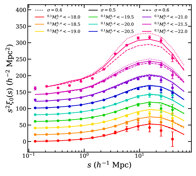
Figure 1: The monopole of the two-point correlation functions from the Uchuu box galaxy catalogue at $z=0.093$ (solid lines) and the SDSS data (filled symbols) for several volume-limited samples corresponding to luminosity cuts as listed in Table 1. For clarity, lines corresponding to different luminosity cuts have been offset by successive intervals $20\text{\,}{\mathrm{\mathit{h}}}^{-2}\text{\,}{\mathrm{Mpc}}^{2}$, starting from the lowest luminosity sample. The clustering is shown for different values of the scatter parameter $\sigma=\{0.4,0.5,0.6\}$, by the dotted, sold and dashed curves, respectively.

The value of $\sigma$ is calibrated to reproduce the observed SDSS galaxy clustering. For more details about the calibration of $\sigma$ and its effect on galaxy clustering, we direct the reader to Appendix B. We also recover the target LF by construction.

The resulting relation between $V_{\mathrm{peak}}$ and ${}^{0.1}M_{r}^{h}$ is shown in Fig. 2 for galaxies with ${}^{0.1}M_{r}<-14.0$ in the $z=0.093$ box. The large volume of Uchuu allows to reach a huge dynamical range in galaxy luminosity $-23<{}^{0.1}M_{r}^{h}<-14$.

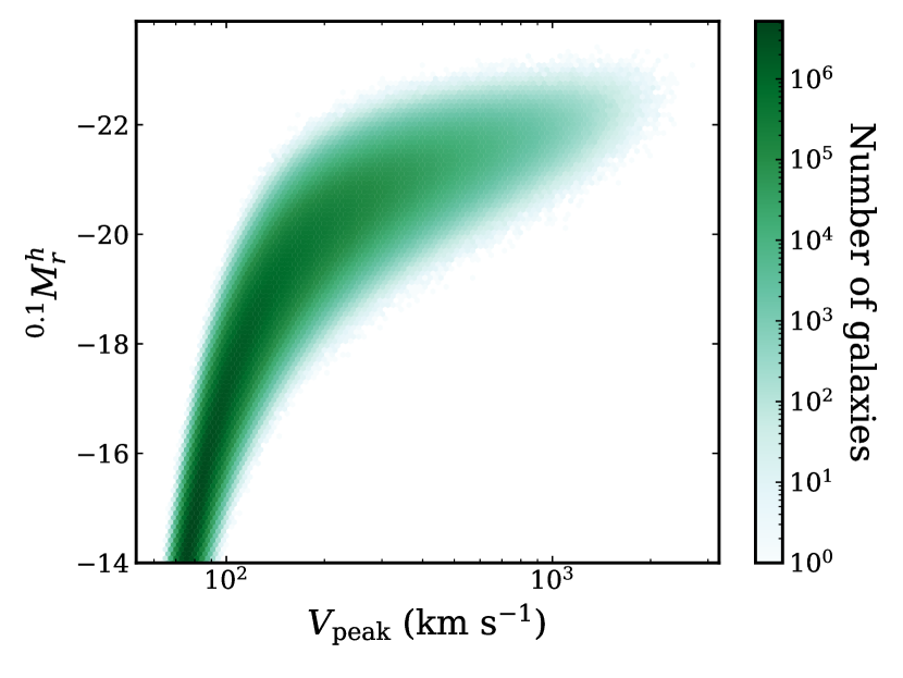
Figure 2: The $(V_{\mathrm{peak}},{}^{0.1}M_{r}^{h})$ distribution in the Uchuu $z=0.093$ box, assuming a constant scatter parameter $\sigma=0.5$. Colour indicates the number of galaxies in each hexagonal bin, in logarithmic scale.

3.3 Uchuu-SDSS galaxy lightcones

We use a total of 6 snapshots between $z=0$ and $z=0.5$, which are separated in redshift by approximately 0.1 ($z_{\mathrm{snap}}=0,0.093,0.19,0.3,0.43,0.49$). Lightcones are created from the snapshots by joining them together in spherical shells. An observer is first placed in the box, and the Cartesian galaxy coordinates in each snapshot are converted to equatorial coordinates, and the redshift is calculated, taking into account the line-of-sight velocity. In each simulation snapshot, galaxies in the redshift range $(z_{\mathrm{snap-1}}+z_{\mathrm{snap}})/2<z<(z_{\mathrm{snap}}+z_{\mathrm{snap+1}})/2$ are selected, which are then joined together to build the lightcone. If the redshift shell is too big to fit inside a single cubic box, periodic replications are applied. In the final lightcone there are no periodic replications below $z=0.36$.

The full-sky lightcone is then cut to the northern contiguous region of the SDSS survey footprint, using a healpix map (Gorski et al., 1999; Blanton et al., 2005; Swanson et al., 2008). The original healpix map has $N_{\mathrm{side}}=512$, but we increase the size of the pixels, using $N_{\mathrm{side}}=128$, and keeping pixels where the completeness in the data is greater than 0.9. This results in a footprint with area $7261~{}\mathrm{deg}^{2}$. The SDSS footprint can be replicated across the full sky to create 4 independent SDSS simulated catalogues. By generating lightcones from eight observer positions (with coordinates at either 0 or $1~{}h^{-1}\mathrm{Gpc}$, along each of the three dimensions), we are therefore able to create a total of 32 Uchu-SDSS lightcones. The first 8 mocks (constructed with observer at the origin, and at the centre of the box) are independent below $z=0.3$. There is some overlap in the volume between the lightcones at higher redshifts than this, but the fraction of galaxies with $z>0.3$ is very small ($\sim 0.1\%$). We refer to these lightcones as the 8 independent lightcones. The full set of 32 lightcones are independent below $z=0.175$, and we use all 32 to improve the statistics of our RSD and BAO measurements (see Section 5). The BAO galaxy sample (eq. 4) has a maximum redshift of $z=0.2$, so there is some overlap between mocks, and $\sim 25\%$ of galaxies in the sample have $z>0.175$.

Combining multiple snapshots in this way to construct a lightcone has the issue that there are discontinuities at the boundaries between snapshots. It is possible for the same halo to appear twice at either side of the boundary, or to not appear at all, and the duplicated haloes artificially boost the pair counts on very small scales. We investigate this in Smith et al. (2022a), and find that there is a boost in the real-space clustering on small scales due to this effect. In redshift space, when velocities are included, the effect is greatly reduced. Using snapshots separated by $\sim 0.1$ in redshift is a good compromise which adds evolution to the lightcone, without excessively boosting the clustering below $1~{}h^{-1}\mathrm{Mpc}$. The clustering measurements on the scales used in a typical RSD analysis ($\gtrsim 20~{}h^{-1}\mathrm{Mpc}$) are insensitive to the number of snapshots used.

3.3.1 Magnitude evolution

Each simulation snapshot was constructed to reproduce the target luminosity function at the redshift of the snapshot, $z_{\mathrm{snap}}$. In the lightcone, this leads to discontinuities in these properties at the boundaries between snapshots.

In order to create a simulated lightcone with a smoothly evolving luminosity function, and smooth $n(z)$, we rescale the galaxy absolute magnitudes as a function of redshift. The original magnitude assigned to each galaxy is first mapped to the corresponding number density, using the luminosity function at $z_{\mathrm{snap}}$. This number density can then be mapped back to an absolute magnitude at the redshift of the galaxy in the lightcone, $z$, using the target luminosity function at the same redshift, $z$. By construction, this reproduces the smooth evolution of the target luminosity function.

3.3.2 Colour assignment

After galaxy luminosities have been assigned, we add ${}^{0.1}(g-r)$ colours to our simulated galaxy sample. We use an evolving empirical model for the ${}^{0.1}(g-r)$ colours, based on (Skibba & Sheth, 2009; Smith et al., 2017), but improved to better reproduce the colour-magnitude diagram from the GAMA survey, at a range of redshifts (Smith et al., 2022b). The bi-modality of the colour probability distribution functions is modelled as a sum of two Gaussian distributions. Defining $p({}^{0.1}(g-r);{}^{0.1}M_{r}^{h},z)\equiv dN/N/d{}^{0.1}(g-r)$, where $N$ is the number of galaxies,

$$\begin{split}p({}^{0.1}(g-r);{}^{0.1}M_{r}^{h},z)&=f_{\mathrm{blue}}\,\mathcal{N}_{\mathrm{blue}}(\mu_{\mathrm{blue}},\sigma_{\mathrm{blue}})\\ &+(1-f_{\mathrm{blue}})\,\mathcal{N}_{\mathrm{red}}(\mu_{\mathrm{red}},\sigma_{\mathrm{red}}),\end{split}$$ (13)

where $\mathcal{N}_{\mathrm{blue}}$ and $\mathcal{N}_{\mathrm{red}}$ are Gaussian probability distribution functions corresponding to blue and red galaxies, respectively, and $f_{\mathrm{blue}}$ is the fraction of blue galaxies. The parameters describing this double-Gaussian distribution all depend on ${}^{0.1}M_{r}^{h}$ and $z$.

At a fixed redshift, the mean and rms of each Gaussian, $\mu_{\mathrm{red}}({}^{0.1}M_{r}^{h})$, $\sigma_{\mathrm{red}}({}^{0.1}M_{r}^{h})$, $\mu_{\mathrm{blue}}({}^{0.1}M_{r}^{h})$ and $\sigma_{\mathrm{blue}}({}^{0.1}M_{r}^{h})$, are modelled as broken linear functions. These functions were fit to the colour-magnitude diagram measured in GAMA, in several redshift bins, which we then interpolate between. Basing the colour distributions on the data from GAMA allows us to create simulated galaxy catalogues to very faint magnitudes, which will be useful e.g. for the DESI Bright Galaxy Survey.

However, we find good agreement between these colours and the measurements from the SDSS data. The fraction of blue galaxies at given luminosity, $f_{\mathrm{blue}}({}^{0.1}M_{r}^{h})$, is modelled differently for central and satellite galaxies. Colours are then drawn randomly from the ${}^{0.1}(g-r)$ colour distributions described above. This method is able to reproduce by construction our target colour distributions.

3.3.3 Apparent magnitudes

The apparent $r$-band magnitude is computed from the absolute magnitude using eq. 1. In the $r$-band, we use a set of colour-dependent $k$-corrections from the GAMA data (see figure 13 of Smith et al., 2017). These are a set of polynomial $k$-corrections, measured in several bins of ${}^{0.1}(g-r)$ colour. These $k$-corrections allow us to calculate apparent magnitudes using the information that was originally available in the simulated catalogue ($r$-band magnitude and $g-r$ colour). In the other bands, we use the $k$-corrections of Blanton et al. (2003a).

We have compared the GAMA and SDSS $r$-band $k$-corrections, and find that the median $k$-corrections at each redshift are in good agreement, differing by no more than $\sim 0.01$. The $1\sigma$ scatter is at a level $<0.04$. At $z=0.1$, both $k$-corrections agree exactly, since ${}^{0.1}k(z=0.1)=-2.5\mathrm{log}_{10}(1.1)\approx-0.103$.

3.3.4 Assigning galaxy properties using SDSS data

The method we have used to create the lightcone assigns each galaxy a rest-frame $r$-band absolute magnitude, ${}^{0.1}M_{r}^{h}$, and ${}^{0.1}(g-r)$ colour. In order to assign more properties to the mock, we match galaxies to the SDSS data. We use a k-d tree to find the closest SDSS galaxy, based on $z$, ${}^{0.1}M_{r}^{h}$ and ${}^{0.1}(g-r)$. Each mock galaxy is then assigned the absolute magnitude in the $u$, $g$, $i$ and $z$-band of the closest-matching galaxy, in addition to its stellar mass and specific star formation rate.

The $u$, $g$, $i$ and $z$-band apparent magnitudes are calculated at the redshift of the mock galaxy from the absolute magnitudes, using eq. 1 and the SDSS $k$-corrections.

3.3.5 Modeling fibre collisions

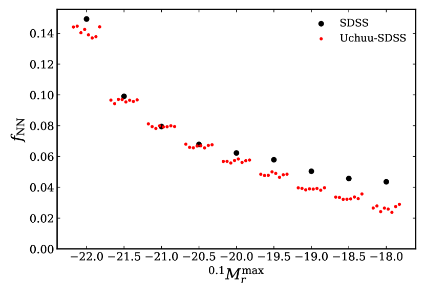
Figure 3: The fraction of galaxies affected by fibre collisions in Uchuu-SDSS and SDSS lightcones. For each of our SDSS volume-limited sample, the black points show the fraction of galaxies receiving the nearest neighbour correction, $f_{\mathrm{NN}}$. The red points show $f_{\mathrm{NN}}$ when we construct volume-limited samples from each of our eight parent Uchuu-SDSS catalogues.

In SDSS, spectroscopic fibres on a single plate cannot be placed closer to each other than the diameter of the fibre plugs. As a result, if two galaxies are in close proximity ($<55^{\prime\prime}$), a spectrum can only be obtained for one of them. The tiling of SDSS plates slightly alleviates this problem, with $\sim 30\%$ of the SDSS footprint covered by multiple plates. These plate ‘overlap regions’ allow for spectroscopic redshifts to be obtained for several galaxies that are within $55^{\prime\prime}$ of one another. Still, $\sim 6\%$ of targeted galaxies in our SDSS sample lack a spectroscopically measured redshift due to their proximity to a neighbouring galaxy.

To mimic the fibre collision effect of SDSS, when constructing our mock galaxy catalogues, we employ a procedure adapted from Szewciw et al. (2022). First, we link together galaxies into friends-of-friends ‘collision groups’. A galaxy is part of a collision group if its angular distance to any galaxy in that group is $<55^{\prime\prime}$. Next, we decide whether each galaxy in a group will be ‘observed’ (i.e. receive its spectroscopic redshift) or ‘unobserved’. When making this choice, we first attempt to maximize the number of galaxies in a collision group that could receive spectroscopic fibres from a single SDSS plate. If there does exist more than one set that maximizes the number of observed galaxies, then we randomly choose one of these sets to be observed. Next, to simulate the effect of SDSS plate overlap regions, we randomly select $\sim 30\%$ of the unobserved galaxies to receive their original observed spectroscopic redshifts. The remaining unobserved galaxies are then assigned the redshift of their angular nearest neighbour. Finally, given the new redshifts of these galaxies, we recompute their $k$-corrections (using the colour-dependent $k$-corrections described in Smith et al., 2017) and absolute magnitudes.

It is important to note that this procedure does not fully mimic the role that plate overlap regions play in recovering the redshifts of collided galaxies. In our procedure the collided galaxies whose redshifts are recovered are chosen at random from the full sky. In SDSS, by contrast, recovered galaxies lie in plate overlap regions and thus are spatially correlated. Furthermore, in SDSS, each overlap region of the sky is covered by a different number of intersecting plates. The number of overlapping plates dictates the number of galaxies whose redshifts can be spectroscopically measured in a given collision group. Our procedure, however, is agnostic with respect to the number of plates required to recover redshifts for any randomly chosen set of collided galaxies.

Despite these differences, we apply the procedure described above to our simulated galaxy catalogues. With this relatively simple procedure described above, the global fraction of galaxies affected by fibre collisions in the simulated lightcone ($f_{\mathrm{NN}}\sim 5.2\%$) is quite similar to that of SDSS ($f_{\mathrm{NN}}\sim 5.9\%$). In Fig. 3, we show a comparison of $f_{\mathrm{NN}}$ between SDSS (black points) and each of our eight independent Uchuu-SDSS lightcones (red points) for the different volume-limited samples defined in Table 1. In both Uchuu and SDSS, we see the same qualitative trend – $f_{\mathrm{NN}}$ increases as we move to more luminous samples. This is as expected, since more luminous galaxies tend to be more strongly clustered and thus are more likely to be affected by fibre collisions. There is good agreement for bright volume-limited samples, although for ${}^{0.1}M_{r}^{\mathrm{max}}\leq-19.5$ Uchuu underestimates $f_{\mathrm{NN}}$ by up to a $2\%$ offset.

After running the fibre assignment algorithm on the 32 Uchuu-SDSS lightcones, we evaluate the fibre assignment completeness in healpix pixels with $N_{\mathrm{side}}=512$. The lightcones are then cut to pixels where the average completeness $>0.9$ (averaged over the 32 lightcones). This results in a final area of $6642~{}\mathrm{deg}^{2}$, which is comparable to the footprint of the SDSS data.

The 32 Uchuu-SDSS lightcone catalogues described in this section, containing ugriz magnitudes, stellar masses, star formation rates and fibre assignment information, are made publicly available at Skies & Universes. A subset of the cubic box catalogues used in the construction of the lightcones, and the companion SDSS data set are also made available. Note that our released box catalogues also include ${}^{0.1}(g-r)$ computed using a similar method as described in Section 3.3.2.

4 Properties of the Uchuu-SDSS galaxies

4.1 Galaxy properties

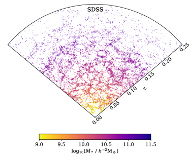
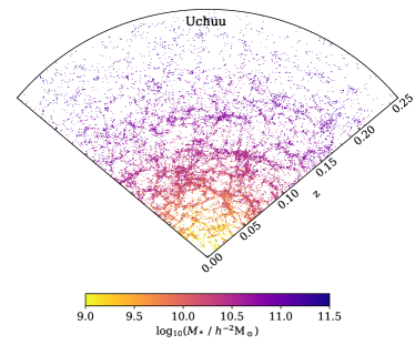
Figure 4: Slice through the SDSS galaxy catalogue (left), and Uchuu-SDSS lightcone (right), where galaxies are coloured by their stellar mass. Galaxies are shown between $35<\mathrm{dec}<40~{}\deg$, and $140<\mathrm{RA}<240~{}\deg$.

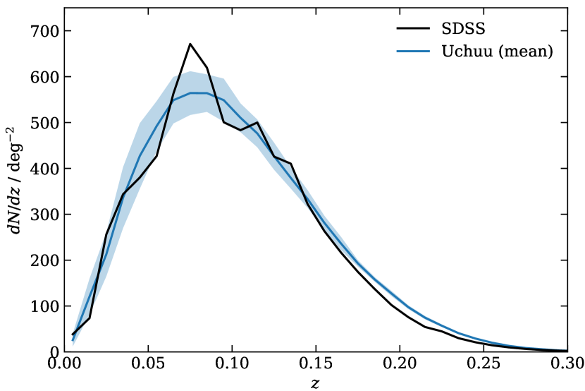
Figure 5: Redshift distribution of galaxies in the the Uchuu-SDSS lightcones, compared to the SDSS data, for galaxies with $r<17.6$. The blue curve is the mean of the 32 simulated lightcones, with the shaded region indicating the $1\sigma$ scatter. The black curve shows the redshift distribution of SDSS. Overall, we find good agreement between Uchuu and SDSS, with a small over-prediction of the number of galaxies in Uchuu at $z\sim 0.2$ due to differences in the luminosity functions.

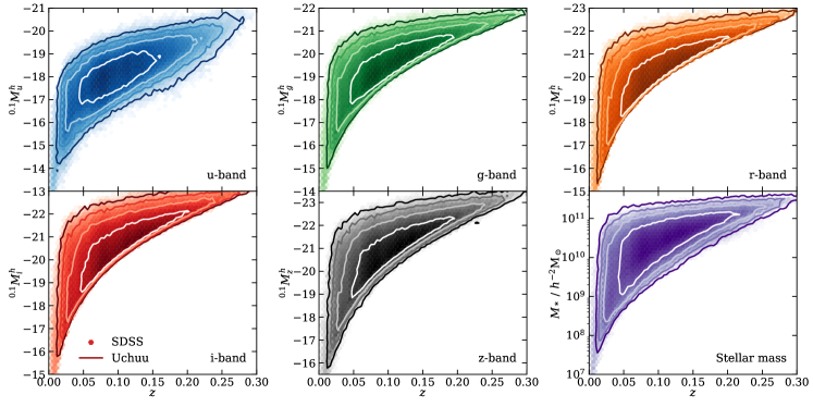
Figure 6: Absolute magnitudes and stellar masses of galaxies in one of the Uchuu-SDSS lightcones (contours), as a function of redshift, compared to the data from SDSS (hexagons), for galaxies with apparent magnitude $r<17.6$. The different panels show the magnitudes in the $ugriz$ bands, as indicated in the legend. The lower right panel shows the MPA stellar masses.

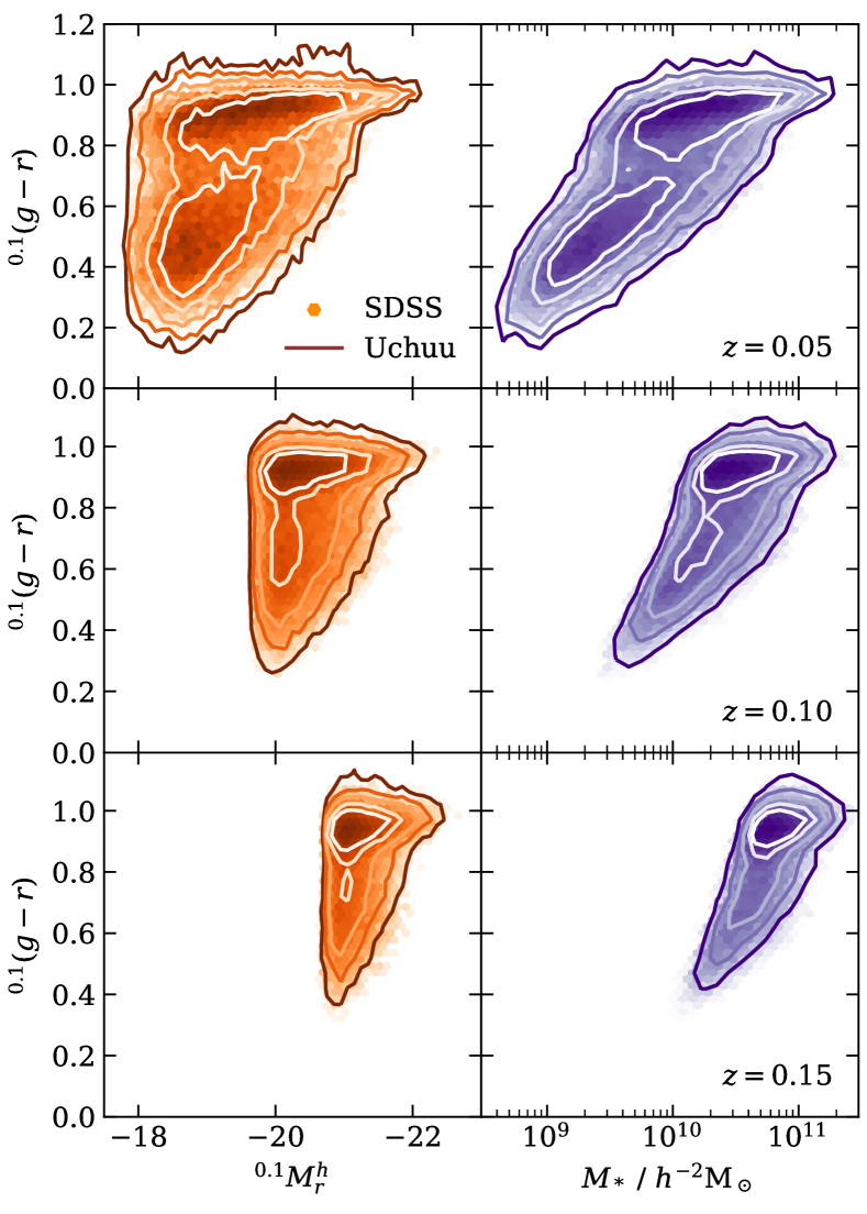
Figure 7: Distribution of ${}^{0.1}(g-r)$ colours in the Uchuu-SDSS lightcone (contours), compared with the colour distributions of SDSS (hexagons). The left-hand column shows the colour distribution with respect to the $r$-band absolute magnitude, at three different redshifts (from top to bottom, $z=0.05$, $z=0.1$ and $z=0.15$). The right-hand column is the same, but with respect to the MPA stellar mass.

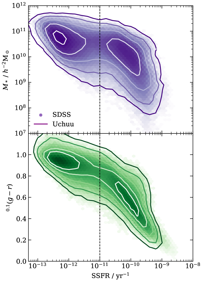
Figure 8: Top panel: stellar mass vs sSFR for galaxies in SDSS (hexagons) and in the Uchuu-SDSS lightcone (contours). Bottom panel: the ${}^{0.1}(g-r)$ colour vs sSFR. The vertical dashed line indicates the sSFR cut of $10^{-11}~{}\mathrm{yr}^{-1}$, which we use to split the bimodal distributions into samples of quiescent and star-forming galaxies.

In this section, we illustrate the various galaxy properties stored in the Uchuu-SDSS lightcones, and compare with the galaxy properties in the SDSS data.

Fig. 4 shows galaxies in a thin slice of the SDSS catalogue and one of the Uchuu-SDSS lightcones, where each galaxy has been coloured based on its stellar mass, illustrating the similarities between the mock and data. The density of galaxies falls with increasing redshift, since faint galaxies with low stellar masses can only be observed close to $z=0$, while the brightest galaxies can be observed over the full redshift range. The density of galaxies appears to be in good agreement between the Uchuu-SDSS and SDSS data.

This can been seen quantitatively in Fig. 5, which compares the redshift distribution of the 32 Uchuu-SDSS lightcones with SDSS. The Uchuu-SDSS lightcones are in good agreement with SDSS, peaking at $z\sim 0.08$. There is scatter between the 32 lighcones, due to cosmic variance, but the measurement from SDSS is consistent with this scatter. At higher redshifts ($z\sim 0.2$), there is a slight excess of galaxies in the Uchuu-SDSS lightcones compared to the data, due to differences in the luminosity function. While the target luminosity function used to construct the simulated lightcones is in good agreement with the SDSS data at low redshifts, we transition to the luminosity function measured in GAMA at higher redshifts. Using the GAMA luminosity function results in a higher number density of galaxies compared to the SDSS measurements, but the SDSS luminosity function is poorly constrained at this redshift.

The absolute magnitudes of galaxies from one of the Uchuu-SDSS lightcones is shown in Fig. 6, compared to SDSS. In the $r$-band, magnitudes were assigned to each galaxy to match an evolving target luminosity function from SDSS and GAMA measurements, and we find that this is able to reproduce well the distribution of absolute $r$-band magnitudes in the SDSS data. The magnitudes in the other bands were assigned by matching each simulated galaxy to a galaxy in the data, based on $r$-band magnitude, $g-r$ colour and redshift. By construction, the distribution of these magnitudes is also in good agreement with the SDSS data.

The ${}^{0.1}(g-r)$ colour distributions in the Uchuu-SDSS lightcones are shown in the left-hand column of Fig. 7, as a function of ${}^{0.1}M_{r}^{h}$, in three narrow redshift bins at $z=0.05$, $z=0.1$ and $z=0.15$. In each redshift bin, the colour distribution is bimodal, with a red sequence of galaxies and cloud of blue galaxies. The brightest galaxies are red, while fainter galaxies have a higher blue fraction. The colour distributions show good agreement with the SDSS data, reproducing the same colour evolution with redshift. There is a small discrepancy at low redshifts, where the red sequence is more sloped in Uchuu-SDSS compared to in SDSS, since the colours in the Uchuu-SDSS lightcone were tuned to GAMA measurements. The right-hand column shows the same colour distributions but as a function of the stellar mass. Here we see that the blue galaxies tend to have lower stellar masses than the red galaxies. Again, there is good agreement between the simulated and real data, with a slight discrepancy in the red sequence at low redshifts.

The distribution of star formation rates of galaxies in the lightcone is shown in Fig. 8, in comparison to the SDSS measurements. The upper panel shows stellar mass against sSFR, while ${}^{0.1}(g-r)$ is plotted against sSFR in the lower panel. There is a clear bimodal distribution of quiescent galaxies with low star formation rates on the left, and star-forming galaxies on the right. The quiescent galaxies tend to have higher stellar masses than the star-forming galaxies. Applying a cut of $10^{11}~{}\mathrm{yr}^{-1}$ in sSFR is able to cleanly cut the galaxy catalogue into these two samples, while we can see in the lower panel that a cut in ${}^{0.1}(g-r)$ would not work as well.

4.2 Luminosity, mass and colour dependence of clustering

In this section, we compare the clustering in our Uchuu-SDSS lightcones with the observational results from the volume-limited SDSS samples. We measure the first non-zero Legendre multipoles ($\ell=0,2,4$) of the redshift-space two-point correlation function (TPCF), defined as,

$$\xi_{\ell}(s)=\left(2\ell+1\right)\int_{0}^{1}\xi^{s}\left(s,\mu\right)L_{\ell}(\mu)d\mu,$$ (14)

where $s=|\mathbf{s}|$, $\mu=\pi/s$ is the cosine of the angle between the line-of-sight direction and the pair separation vector $\mathbf{s}$. $\xi^{s}\left(s,\mu\right)$ is the two point correlation function and $L_{\ell}$ is the $\ell^{\mathrm{th}}$-order Legendre polynomial. These quantities are computed using the publicly available code FCFC (Zhao et al., 2021).

Fig. 9 compares the monopole, $\xi_{0}(s)$, quadrupole, $\xi_{2}(s)$, and hexadecapole, $\xi_{4}(s)$, of the TPCF of 8 independent Uchuu-SDSS lightcone catalogues against the measurements from the SDSS dataset, for the set of volume-limited samples described in Table 1. The clustering of our Uhuu-SDSS galaxies is in good agreement with the data for all the volume-limited samples considered, despite the simplicity of our luminosity assignment model – note that we neglect any potential dependence of our scatter parameter on redshift or luminosity, and consequently our luminosity assignment model has only one tunable parameter. The agreement is poorer for the ${}^{0.1}M_{r}^{h}<-22$ sample, with the Uchuu-SDSS lightcones underestimating the observed monopole. This suggests that the scatter between our halo mass proxy and galaxy luminosity is likely to decrease for bright galaxies ${}^{0.1}M_{r}^{h}\lesssim-22$, which is in agreement with previous findings (Stiskalek et al., 2021).

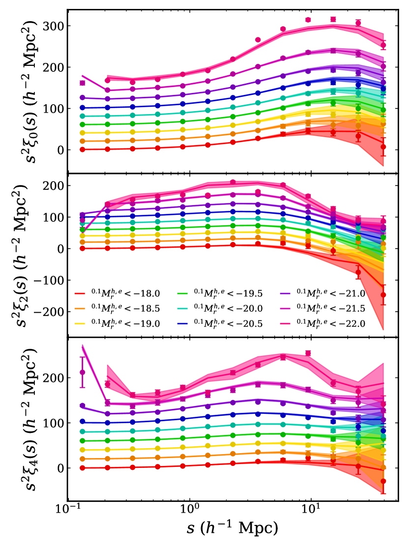
Figure 9: Monopole (top panel), quadrupole (middle panel) and hexadecapole (bottom panel) of the TPCF of Uchuu-SDSS and SDSS galaxies for several volume-limited samples corresponding to luminosity cuts (see Table 1). Solid lines indicate the average of the eight independent Uchuu-SDSS lightcones, while the shaded regions indicate the rms scatter. Data points indicate the clustering measured from the SDSS sample described in Section 2. For clarity, lines corresponding to different luminosity cuts have been offset by successive intervals $20\text{\,}{\mathrm{\mathit{h}}}^{-2}\text{\,}{\mathrm{Mpc}}^{2}$, starting from the lowest luminosity sample. Note that the lowest-$s$ point for the ${}^{0.1}M_{r}^{h}<-22$ sample has been removed due to low statistics.

Similarly, Fig. 10 shows the two-point correlation function for several $M_{\ast}$ cuts. We find again good agreement between our simulated catalogues and the SDSS data. The poorer agreement for the highest mass cut at $\log_{10}(M_{\ast})>11$ suggests again a decrease in the scatter in the galaxy–halo connection at the high mass end, in agreement with previous studies (Behroozi et al., 2019).

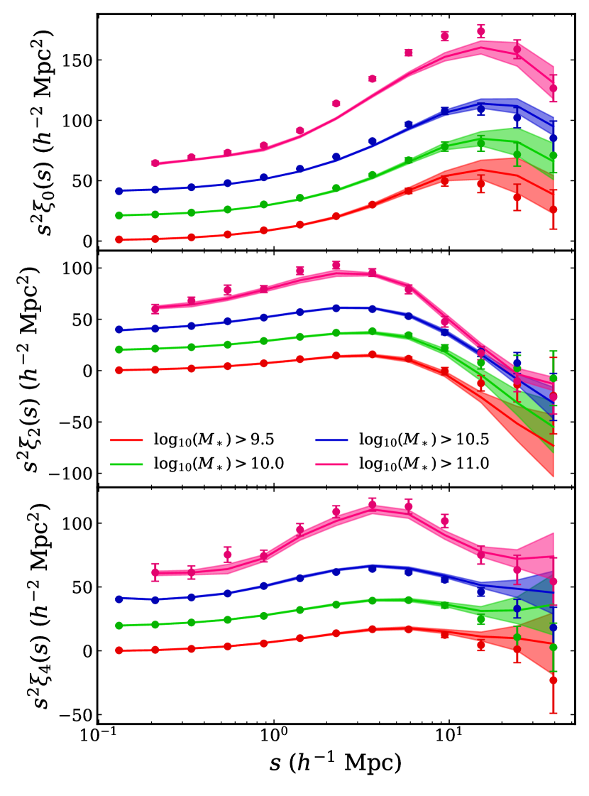
Figure 10: Similar to Fig. 9. Here, the clustering for several $M_{\ast}$ cuts are depicted. For clarity, lines corresponding to different cuts have been offset by successive intervals $20\text{\,}{\mathrm{\mathit{h}}}^{-2}\text{\,}{\mathrm{Mpc}}^{2}$, starting from the lowest mass sample. Note that the lowest-$s$ point for the $\log_{10}(M_{\ast})<11.0$ sample has been removed due to low statistics.

In order to study the colour-dependence of clustering, we split the sample into two populations of blue and red galaxies. We use a luminosity-dependent colour cut as introduced in Zehavi et al. (2005), (eq. 13 in Zehavi et al., 2011).

$${}^{0.1}(g-r)_{\mathrm{cut}}=0.21-0.03~{}{}^{0.1}M_{r}^{h,e}.$$ (15)

Galaxies above the ${}^{0.1}(g-r)$ cut belong to the red population, while galaxies below the cut belong to the blue population.

Fig. 11 compares the TPCF for blue, red and all galaxies of Uchuu-SDSS with that of the SDSS dataset, for a subset of the volume-limited samples in Table 1.

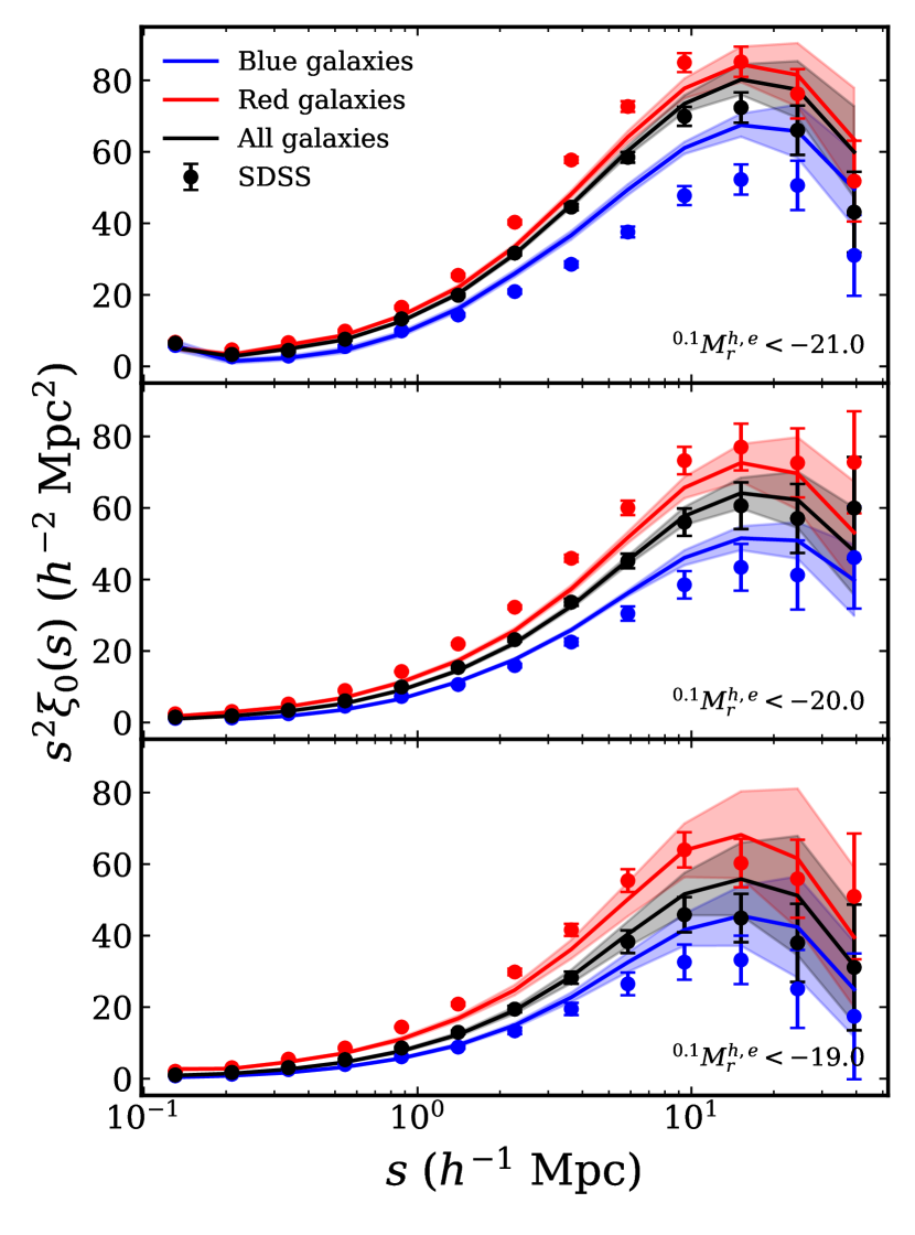
Figure 11: The monopole of the two-point correlation function for SDSS (points with error bars) and Uchuu-SDSS galaxies (solid lines), split into blue and red galaxies according to eq. 15. The dark solid lines indicate the average of the eight independent Uchuu-SDSS lightcones, while the shaded regions show the rms scatter. Each panel corresponds to a volume-limited sample, as indicated in the lower right corner.

Uchuu-SDSS is in reasonable agreement with the SDSS data, although the agreement is visibly poorer than for the overall volume-limited samples, specially for the brightest samples. This points to limitations due to the simplicity of our colour-assignment algorithm. As described in Section 3.3.1, colours in the lightcone are randomly drawn from our target colour distribution. Our results could be improved, by using information about the halo age to assign colours, thus accounting for assembly bias. This would likely require to apply a model involving free parameters, which would need to be finely tuned in order to match the observed colour-dependent clustering.

4.3 Stellar mass function

In order to further validate our simulated galaxy catalogues, we calculate the stellar mass function (SMF) of the SDSS sample (see Section 2.2) and compare it with that from the set of 8 independent Uchuu-SDSS lightcones (see Section 3.3.4). The SMF is estimated by the non-parametric $1/V_{\mathrm{max}}$ method widely used in deriving the galaxy luminosity function. To compute the SMF for SDSS and Uchuu samples, we select all galaxies in a redshift range of $0.02\leq z\leq 0.2$ with stellar masses $M_{\ast}\geq 10^{9}~{}h^{-2}\mathrm{M_{\odot}}$ and $r$-band apparent magnitudes $14.5\leq r\leq 17.6$.

In Fig. 12 (left panel), we present the SMF obtained from the mean of the 8 Uchuu-SDSS lightcones. Results are compared to SMF derived from the SDSS sample. We also compare our results with that obtained by Moustakas et al. (2013). In Moustakas et al. (2013), $M_{\ast}$ was determined utilizing iSEDfit, a suite of routines used to determine stellar masses, SFRs, and other physical properties of galaxies from the observed broadband SEDs and redshifts (e.g. Kauffmann et al., 2003; Salim et al., 2007). The Uchuu-SDSS is in reasonably good agreement with both MPA-SDSS and SMF obtained by Moustakas et al. (2013).

The middle and right panels of Fig. 12 show the SMF of quiescent and star-forming galaxies for each data set. We adopt $\mathrm{sSFR}=10^{-11}~{}\mathrm{yr}^{-1}$ as the threshold between quiescent and star-forming galaxies. This value corresponds to the minimum between the two peaks of the bimodal sSFR distribution shown in Fig. 8. The Uchuu-SDSS SMFs for quiescent and star-forming galaxies galaxies is consistent with those obtained from MPA-SDSS for all masses, although for quiescent galaxies the agreement is slightly poorer compared to the overall sample in the left panel. There is also a good agreement between the Uchuu SMFs and those obtained by Moustakas et al. (2013), with a notable offset at the low- and high-mass ends for quiescent galaxies. One possible reason for this difference is the different methods for the estimation of SFRs used by MPA/JHU and Moustakas et al. (2013), which result in different SFR values.

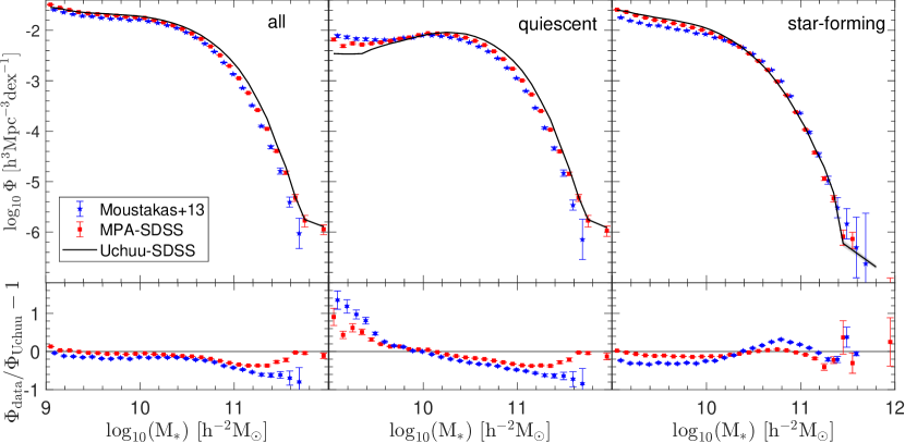
Figure 12: Comparison of the SMF of the Uchuu-SDSS data (the mean of the 8 independent lightcones) with that obtained from the SDSS data with $0.02\leq z\leq 0.20$, $\mathrm{M_{\ast}}\geq 10^{9}~{}h^{-2}M_{\odot}$, and $14.5\leq r\leq 17.6$, in addition to the results from MPA and Moustakas et al. (2013), as shown in the legends. Left, middle and right panels present the SMF for all, quiescent, and star-forming galaxies, respectively. The lower panels show the relative fraction, $\Phi_{\mathrm{data}}/\Phi_{\mathrm{Uchuu}}-1$, of the SMF relative to that from Uchuu-SDSS. The plot shows a reasonable agreement among all three data sets, except for quiescent galaxies at the low- and high-mass ends.

4.4 Halo occupation distribution

Galaxies are known to be biased tracers of the underlying dark matter density field. In order to better understand the connection between galaxies and haloes in Uchuu-SDSS catalogues, we investigate the halo occupation distribution. We compute $\langle N_{\mathrm{gal}}(>L|M_{\mathrm{halo}})\rangle$ – the mean number of galaxies brighter than a given $r$-band luminosity in a halo with virial mass $M_{\mathrm{halo}}$.

The luminosity-dependent HOD is modeled with the functional form described in Zehavi et al. (2011). We write $\langle N_{\mathrm{gal}}(>L|M_{\mathrm{halo}})\rangle$ as a sum of the mean number of central and satellite galaxies. The mean occupation function of the central galaxies is modelled as a step-like function with a cutoff profile softened to account for the scatter between galaxy luminosity and halo mass, and the mean occupation of satellite galaxies is modelled as a power law modulated by a similar cutoff profile, see Zehavi et al. (2011) for the details. This HOD model has five free parameters: the mass scale, $M_{\mathrm{min}}$, and width, $\sigma_{\log{M}}$, of the central galaxy mean occupation, and the cutoff mass scale, $M_{0}$, normalization, $M_{1}^{\prime}$, and high-mass slope, $\alpha$, of the satellite galaxy mean occupation function.

We fit this model to the average HOD obtained from 8 independent Uchuu-SDSS lightcones for the volume-limited samples corresponding to luminosity cuts described in Table 1. The best fitting HOD parameters are shown in Table 3, along with the SDSS estimates from Zehavi et al. (2011). Fig. 13 shows the mean halo occupation of the Uchuu-SDSS galaxies and the best-fit HOD models. As seen in the figure, the HOD shifts towards more massive haloes as the luminosity threshold increases – more luminous galaxies occupy more massive haloes.

Our results broadly agree with those of Zehavi et al. (2011) over the wide range of brightness thresholds for all volume-limited samples. However, we observe a few discrepancies for some HOD parameters (see Table 3). This is likely due to the difference in the methodologies. While we have computed the halo occupation directly from our values of ${}^{0.1}M_{r}^{h}$ and $M_{\mathrm{halo}}$ in the Uchuu-SDSS lightcones, Zehavi et al. (2011) obtains it by fitting the projected correlation function of the observed SDSS data. All our best fit parameters, except $\alpha$, follow an ascending trend as a function of the luminosity threshold.

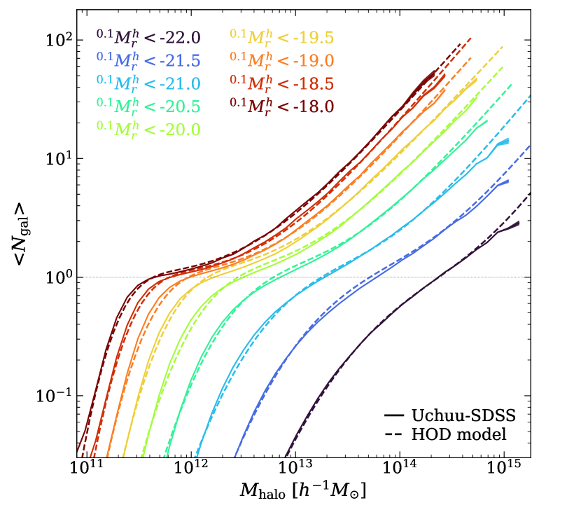
Figure 13: Measured mean halo occupation for the different luminosity threshold samples drawn from 8 independent Uchuu-SDSS lightcones as a function of halo mass. The dashed lines represents the best-fit models for the halo occupation functions. Best-fit HOD parameters are shown in Table 3 together with those obtained by Zehavi et al. (2011). The maximum host halo mass in each sample is related to their effective volume (see Table 1).

${}^{0.1}M_{r}^{\mathrm{max}}$	$\log{M_{\mathrm{min}}}$	$\sigma_{\log{M}}$	$\log{M_{0}}$	$\log{M_{1}^{\prime}}$	$\alpha$
-18.0	11.34$\pm$0.09	0.29$\pm$0.20	11.07$\pm$0.08	12.60$\pm$0.03	0.99$\pm$0.03
	11.18	0.19	9.81	12.42	1.04
-18.5	11.48$\pm$0.08	0.31$\pm$0.16	11.08$\pm$0.07	12.73$\pm$0.04	1.03$\pm$0.03
	11.33	0.26	8.99	12.50	1.02
-19.0	11.66$\pm$0.06	0.35$\pm$0.12	11.16$\pm$0.07	12.83$\pm$0.02	0.99$\pm$0.02
	11.45	0.19	9.77	12.63	1.02
-19.5	11.85$\pm$0.10	0.38$\pm$0.16	11.37$\pm$0.09	12.95$\pm$0.04	0.95$\pm$0.03
	11.57	0.17	12.23	12.75	0.99
-20.0	12.12$\pm$0.08	0.45$\pm$0.11	11.48$\pm$0.09	13.17$\pm$0.04	0.97$\pm$0.04
	11.83	0.25	12.35	12.98	1.00
-20.5	12.43$\pm$0.06	0.52$\pm$0.06	11.49$\pm$0.11	13.47$\pm$0.03	1.00$\pm$0.04
	12.14	0.17	11.62	13.43	1.15
-21.0	12.86$\pm$0.12	0.62$\pm$0.09	11.69$\pm$0.12	13.83$\pm$0.09	1.07$\pm$0.14
	12.78	0.68	12.71	13.76	1.15
-21.5	13.32$\pm$0.14	0.68$\pm$0.09	11.79$\pm$0.14	14.25$\pm$0.09	1.08$\pm$0.16
	13.38	0.69	13.35	14.20	1.09
-22.0	13.98$\pm$0.30	0.81$\pm$0.22	11.86$\pm$0.22	14.76$\pm$0.19	1.26$\pm$0.30
	14.06	0.71	13.72	14.80	1.35

Table 3: Best-fit HOD parameters for our volume-limited samples. For each luminosity cut the top row indicates the best-fit parameters for our Uchuu-SDSS lightcones, while the bottom row shows that for the SDSS data as reported in Zehavi et al. (2011). Error bars on our HOD parameters correspond to standard deviation errors on the parameters. Halo masses are in units of $h^{-1}M_{\odot}$.

5 RSD and BAO measurements

In this section we study the BAO signal in the SDSS MGS. For this purpose we define a BAO sample (SDSSbao, see Section 2.1) in which this signal is enhanced similar to Ross et al. (2015). We also model the full shape of the TPCF to measure $f\sigma_{8}$ and obtain the anisotropic BAO distances. While we have the set of 32 Uchuu-SDSS lightcones to compare with the SDSSbao data, in order to further improve our covariance errors on BAO scales, we generate an additional sample of 5100 light-cones, describe below, using a set of lower resolution $N$-body simulations run with the GLAM code (Klypin & Prada, 2018).

In Section 5.1 we describe the method used to construct our 5100 GLAM-SDSSbao lightcones, while their clustering properties are explored in Section 5.2. Our RSD measurements are presented in Section 5.3. Finally, we measure the isotropic BAO scale in Section 5.4.

5.1 Constructing the GLAM lightcones

We generate 1275 GLAM simulations using the same cosmology and linear power spectrum as the Uchuu simulation. The GLAM simulations follow the evolution of $2000^{3}$ particles of mass $1.07\times 10^{10}h^{-1}\mathrm{M_{\odot}}$ in a cubic box of size $1~{}h^{-1}\mathrm{Gpc}$ with $N_{s}=140$ timesteps, and mesh of $N_{g}=5800$. This numerical set-up yields a spatial resolution of $\Delta x=0.172~{}h^{-1}\mathrm{Mpc}$. The initial conditions are generated using the Zeldovich approximation starting at $z_{\mathrm{ini}}=105$. The distinct haloes in GLAM are identified with the Bound Density Maximum halo finder (Klypin & Holtzman, 1997).

Since the GLAM simulations are unable to resolve substructure inside distinct haloes, the SHAM method introduced in Section 3 cannot be applied, and we thus resort to a statistical HOD method. First, we compute the HOD of the SDSSbao sample by applying the galaxy selection criteria in eq. 4 to our 8 independent Uchuu-SDSS lightcones (hereafter Uchuu-SDSSbao). We then use the 1275 GLAM halo catalogues available at the mean redshift of the BAO sample ($z\sim 0.1$) to generate a galaxy catalogue for each GLAM box by randomly drawing galaxies from the measured halo occupation statistics for each distinct halo. Fig. 14 shows the mean HOD from Uchuu-SDSSbao used to populate with galaxies the GLAM simulations, along with the resulting mean HOD obtained from the 1275 GLAM galaxy catalogues. By construction, the HOD of Uchuu- and GLAM-SDSSbao galaxies are in agreement. It is important to note that the GLAM simulations are only able to resolve haloes larger than $10^{12}~{}h^{-1}\mathrm{M_{\odot}}$. However, the HOD obtained from the high-fidelity Uchuu-SDSSbao lightcones does not extends to masses below this limit. The resulting GLAM galaxy catalogues have an average density of $6\times 10^{-4}$ galaxies per unit volume (average $n(z)$ of the Uchuu-SDSSbao sample).

Once the GLAM halos for a given box are populated with galaxies, we adjust its number density to match that in the SDSSbao sample. For this step, we use the $n(z)$ presented in Ross et al. (2015) as reference. Then we cut it to the northern contiguous region of the SDSS survey footprint. As with the Uchuu lightcones, by replicating the SDSS footprint across the full sky, we can generate a total of 4 independent SDSSbao lightcones from each GLAM box, which allows us to create a total of 5100 GLAM-SDSSbao lightcones. We decided not to apply the fibre collision correction to GLAM-SDSSbao since it effect is negligible on the scales we are going to make use of the lightcones (BAO scales).

The GLAM-SDSSbao lightcones mean number density is shown in Fig. 15 together with that from Uchuu-SDSSbao and the SDSSbao data. There is a 20% slight excess of galaxies in Uchuu-SDSSbao as compared to the data and the GLAM-SDSSbao lightcones at high-redshift tail of the distribution. As explained in section 4.1, this is because we use a target luminosity function to build the Uchuu galaxy catalogues that transitions from SDSS to GAMA, since the luminosity function from SDSS is poorly constrained at high redshifts. This difference does not seem to have a significant impact on the performance of our Uchuu-SBSSbao lightcones in reproducing within $1\sigma$ the SDSSbao clustering, however it may explain the small difference seen between Uchuu- and GLAM-SDSSbao (see Fig. 16).

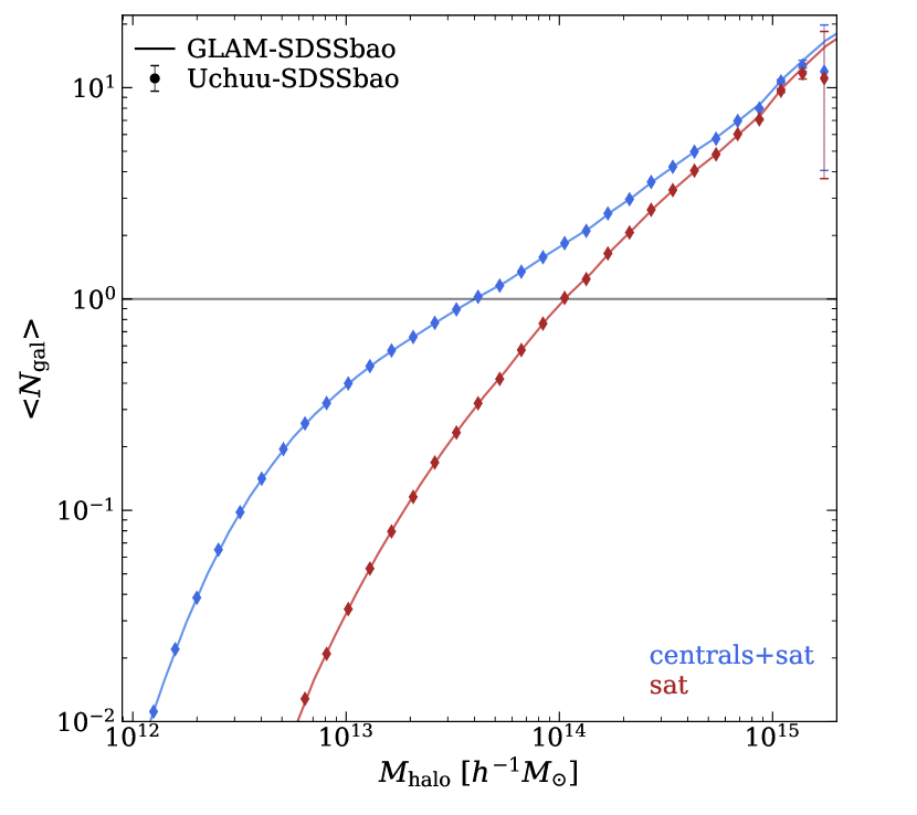
Figure 14: Mean halo occupation distribution from our Uchuu- and GLAM-SDSSbao catalogues, dots and solid line, for all galaxies and satellite galaxies only (in blue and red respectively).

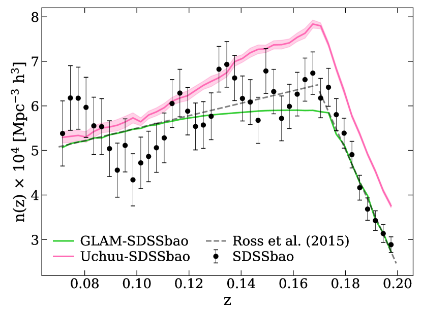
Figure 15: Number density of the SDSSbao data, Uchuu- and GLAM-SDSSbao lightcones. The green line represents the mean $n(z)$ of the 5100 GLAM-SDSSbao, while the magenta represents that from the 32 Uchuu-SDSSbao. The standard deviation for each of the samples is shown as a shaded area. The error bars that accompany the SDSSbao $n(z)$, represented with black dots, are taken from the standard deviation of the GLAM-SDSSbao catalogues. The deviation between GLAM and Ross et al. (2015) around $z=0.16$ follows from the $n(z)$ of GLAM galaxy catalogues obtained from the HOD.

5.2 Two-point correlation function and covariance matrix

In this section we explore the clustering on the BAO scales in the three data sets: SDSSbao, Uchuu- and GLAM-SDSSbao.

In order to optimise the BAO clustering signal-to-noise ratio, we weight both galaxies and randoms depending on the galaxy number density $n(z)$ using FKP weights (Feldman et al., 1994; Ross et al., 2015), i.e.

$$w_{\textrm{FKP}}=\frac{1}{1+P_{\textrm{FKP}}n(z)}.$$ (16)

We set $P_{\textrm{FKP}}=16\,000~{}h^{-3}\mathrm{Mpc}^{3}$ , which is close to the measured amplitude at $k=0.1~{}h^{-1}\mathrm{Mpc}$.

Further, from the 5100 GLAM-SDSSbao lightcones, we infer the covariance matrix, $C$, defined as

$$C^{\ell_{i}\ell_{j}}(s_{i},s_{j})=\frac{1}{N-1}\sum^{N}_{n=1}[\xi^{(\ell_{i})}(s_{i})-\bar{\xi}^{(\ell_{i})}(s_{i})][\xi^{(\ell_{j})}(s_{j})-\bar{\xi}^{(\ell_{j})}(s_{j})],$$ (17)

where $N$ is the number of lightcones.

Fig. 16 shows the monopole, quadrupole and hexadecapole of the two-point correlation function of the SDSSbao data, the mean of the 32 Uchuu-SDSSbao lightcones (described in Section 3.3), and the mean of the 5100 GLAM-SDSSbao. We include all bins between 25 and $200~{}h^{-1}\mathrm{Mpc}$ in $5~{}h^{-1}\mathrm{Mpc}$ steps. The error bars in the SDSSbao TPCF are calculated from the diagonal elements of the GLAM-SDSSbao covariance matrix. For Uchuu and GLAM, we plot the error in the mean of the correlation functions as shaded regions.

The three data sets show a clear BAO peak at $s\sim$100\text{\,}{\mathrm{\mathit{h}}}^{-1}\text{\,}\mathrm{Mpc}$$. Uchuu- and GLAM-SDSSbao generally agree with the SDSSbao observational measurements within $2\sigma$. The GLAM measurements have better statistics than Uchuu, due to the huge number of lightcones in the GLAM suite. Moreover, Uchuu have a larger number density than GLAM, which translates into a lower clustering amplitude. Note that the GLAM lightcones, used to estimate uncertainties from its TPCF covariance matrix, match the SDSSbao number density (see Fig. 15).

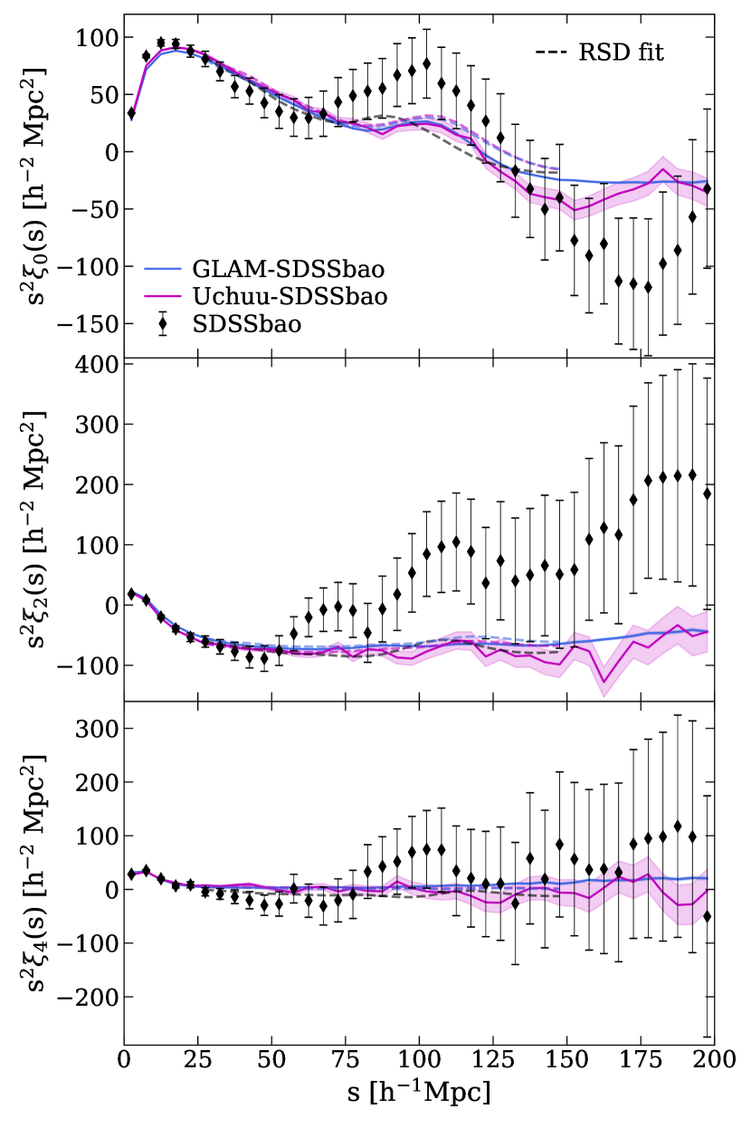
Figure 16: The monopole, quadrupole and hexadecapole of the two-point correlation function measured in our three SDSS BAO data set: SDSSbao (filled symbols), GLAM-SDSSbao (blue lines) and Uchuu-SDSSbao (pink lines). Errors have been estimated from the covariance matrix of the 5100 GLAM-SDSSbao lightcones. Observations and simulated data agree within 2$\sigma$ at all scales. Following the same colour code, we also plot the best-fit RSD model (dashed lines) for each data, (see Section 5.3).

5.3 RSD measurements

Galaxy clustering analyses that rely on two-point statistics are not sensitive to the growth rate of structure $f$ directly but instead to $f\sigma_{8}$, where $\sigma_{8}$ is the normalization of the linear power spectrum on scale of $8~{}h^{-1}\mathrm{Mpc}$.

We measure the linear growth rate of structure, $f\sigma_{8}$, and the Alcock-Paczynski parameters, $\alpha_{\perp}$ and $\alpha_{\parallel}$, of the Uchuu-SDSS lightcones and SDSSbao sample described above using the two-point correlation function, $\xi(s,\mu)$.

The anisotropic Alcock-Paczynski parameters are defined as

$$\alpha_{\parallel}=\frac{D_{\mathrm{H}}(z)r^{\text{fid}}_{d}}{D_{\mathrm{H}}^{\text{fid}}(z)r_{d}}$$ (18)

and

$$\alpha_{\perp}=\frac{D_{\mathrm{M}}(z)r^{\text{fid}}_{d}}{D_{\mathrm{M}}^{\text{fid}}(z)r_{d}},$$ (19)

where $H(z)$ is the Hubble parameter, $D_{\mathrm{M}}(z)$ is the angular diameter distance, $D_{\mathrm{H}}(z)=c/H(z)$ is the Hubble distance, and $r_{d}$ is the sound horizon at the drag epoch. Quantities with a ‘fid’ superscript are calculated for the fiducial cosmology assumed during the analysis, while the quantities without a superscript exist in the true cosmology.

The analysis is performed using the Planck fiducial cosmology, as adopted for Uchuu, to convert the redshifts to comoving distances. If the assumed fiducial cosmology does not match the true cosmology, there is a scaling of the BAO peak position parallel and perpendicular to the line-of-sight (as given in eqs. 18, 19). Thus, we should recover $\alpha_{\perp}=\alpha_{\parallel}=1$ from the Uchuu- and GLAM-SDSSbao lightcones.

From the covariance matrix $C$ computed in section 5.2, we can define the $\chi^{2}$ statistic as

$$\chi^{2}=\frac{N-p-2}{N-1}(\xi^{\text{Data}}-\xi^{\text{Model}})C^{-1}(\xi^{\text{Data}}-\xi^{\text{Model}})^{T},$$ (20)

where $p$ is the number of degrees-of-freedom being fitted and $N$ is the number of GLAM-SDSSbao lightcones, and we have included the Hartlap correction (Hartlap et al., 2007).

Our theoretical model for the TPCF, $\xi^{\text{Model}}$, is based on Lagrangian Perturbation Theory (LPT). To model the distribution of galaxies, one also needs to introduce a bias model that connects the matter density, $\delta_{m}$, and the galaxy density, $\delta_{g}$. with two parameters $b_{1}$ and $b_{2}$ named the linear and quadratic Lagrangian bias, respectively. We can then obtain the model power spectrum, and include the effect of peculiar velocities to account for the RSD effect (Seljak & McDonald, 2011).

We also model the Fingers-of-God (FOG) effect in Fourier space, using the phenomenological Lorentz model (Taruya et al., 2010):

$$P_{\mathrm{FOG}}(\boldsymbol{k})=\frac{1}{1+(\boldsymbol{k}\cdot\hat{\boldsymbol{n}}\>\sigma_{\mathrm{FOG}})^{2}/2}P(\boldsymbol{k}).$$ (21)

where $P(\boldsymbol{k})$ is the non-linear power spectrum without the FOG effect, $\sigma_{\mathrm{FOG}}$ is the one-dimensional velocity dispersion and $\hat{\boldsymbol{n}}$ is the normalised LOS direction vector.

The theoretical power spectrum $P_{\mathrm{FOG}}$ is obtained using the MomentumExpansion module of velocileptors package (for more details, see Chen et al., 2020; Chen et al., 2021). Finally, we obtain the correlation function by taking the Fourier transform of $P_{\mathrm{FOG}}$,

$$\xi(\boldsymbol{x})=\int d^{3}\boldsymbol{k}e^{i\boldsymbol{k}\cdot\boldsymbol{x}}P_{\mathrm{FOG}}(\boldsymbol{k}).$$ (22)

We fit our RSD model to the correlation function multipoles from three datasets SDSSbao, Uchuu-SDSSbao and GLAM-SDSSbao in the separation range $[25,145]~{}h^{-1}\mathrm{Mpc}$, with bins of width $5~{}h^{-1}\mathrm{Mpc}$. In addition to the cosmological parameters $f\sigma_{8}$, $\alpha_{\parallel}$ and $\alpha_{\perp}$, we also estimate the Lagrangian biases $b_{1},b_{2}$ and the Fingers-of-God parameter $\sigma_{\mathrm{FOG}}$. Unphysical values of parameters are avoided by setting the priors to $f\sigma_{8}>0$, $b_{1}>-1$ and $\sigma_{\mathrm{FOG}}>0$. The first Lagrangian bias is related to the Eulerian bias by $b_{1,\rm Eulerian}=1+b_{1}$. We assume the effective redshift of the SDSSbao sample to be $z=0.15$.

The correlation function multipoles corresponding to our best-fit models can be seen in Fig 16. We observe good agreement with Uchuu-SDSSbao and GLAM-SDSSbao measurements. The RSD model predicts position of the BAO peak in the monopole that is too low as compared with the observed position of the peak. However, this disagreement is within the noise limits.

The minima of $\chi^{2}$ is found using iminuit (Dembinski & et al., 2020), which achieves convergence near the minimum using the first and approximate second derivatives. Errors are estimated from the region of $\Delta\chi^{2}=1$ of the marginalized $\chi^{2}$ distribution, and they are allowed to be asymmetric. We also run Monte Carlo Markov chains (MCMC) with the emcee package (Foreman-Mackey et al., 2013) in order to compute the likelihood surface of our set of fitted parameters. Their convergence is checked with the Gelman-Rubin convergence test (Gelman & Rubin, 1992; Brooks & Gelman, 1998).

We first test our RSD pipeline on the GLAM-SDSSbao and Uchuu-SDSSbao light-cones. The best-fit results of the parameters $f\sigma_{8}$, $\alpha_{\parallel}$ and $\alpha_{\perp}$ are summarised in Fig. 17. We confirm that the theoretical model recovers the fiducial Planck values within 1$\sigma$.

We then apply the pipeline to the SDSSbao sample. Our results are listed in Table 4. Both $\chi^{2}$ minimization and MCMC sampling methods provide consistent results, and the small difference in the errors and parameter values are attributed to a better treatment of the Fingers-of-God effect with MCMC chains. The parameter distributions for $\sigma_{\mathrm{FOG}}$ is non-Gaussian, as it is restricted to positive values, but the best-fit value is consistent with 0. Additionally, we compare our obtained $f\sigma_{8}$ and $b_{1}$ with Howlett et al. (2015), finding a good agreement, but we obtain a $\gtrsim 30\%$ increase in precision on $f\sigma_{8}$ which it can be attributed to our better estimate of the covariance matrix (see Table 4).

Parameter	$\chi^{2}$ minimization	MCMC	Reference
$f\sigma_{8}$	$0.65^{+0.17}_{-0.16}$	$0.62^{+0.17}_{-0.17}$	$0.63^{+0.24}_{-0.27}$
$\alpha_{\parallel}$	$0.99^{+0.11}_{-0.10}$	$1.04^{+0.15}_{-0.10}$	N/A
$\alpha_{\perp}$	$1.18^{+0.10}_{-0.08}$	$1.17^{+0.07}_{-0.07}$	N/A
$b_{1,\rm Eulerian}$	$1.59^{+0.19}_{-0.19}$	$1.62^{+0.22}_{-0.19}$	$1.36^{+0.29}_{-0.26}$
$b_{2}$	$-0.3^{+2.1}_{-1.6}$	$-0.8^{+1.6}_{-1.4}$	N/A
$\sigma_{\mathrm{FOG}}[h^{-1}\mathrm{Mpc}]$	$4.5^{+2.8}_{-4.5}$	$3.6^{+2.5}_{-3.5}$	N/A

Table 4: RSD fitted parameters from the SDSSbao data, obtained by $\chi^{2}$ minimization and using Bayesian MCMC inference. Only $f\sigma_{8}$ and $b_{1,\rm Eulerian}$ estimated values from Howlett et al. (2015) are found in the literature.

Parameter	Uchuu	GLAM	Expected value
$f\sigma_{8}$	$0.48^{+0.15}_{-0.15}$	$0.45^{+0.16}_{-0.16}$	$0.46$
$\alpha_{\parallel}$	$0.94^{+0.11}_{-0.09}$	$0.94^{+0.16}_{-0.10}$	1.00
$\alpha_{\perp}$	$0.99^{+0.08}_{-0.07}$	$1.00^{+0.09}_{-0.08}$	1.00
$b_{1,\rm Eulerian}$	$1.42^{+0.17}_{-0.15}$	$1.40^{+0.19}_{-0.17}$	N/A
$b_{2}$	$-0.4^{+1.6}_{-1.3}$	$-0.6^{+1.6}_{-1.3}$	N/A
$\sigma_{\mathrm{FOG}}[h^{-1}\mathrm{Mpc}]$	$0^{+9}_{-0}$	$0^{+22}_{-0}$	N/A

Table 5: RSD fitted cosmological parameters from the means of Uchuu and GLAM correlation functions, obtained using $\chi^{2}$ minimization in comparison with the values predicted by the fiducial cosmology.

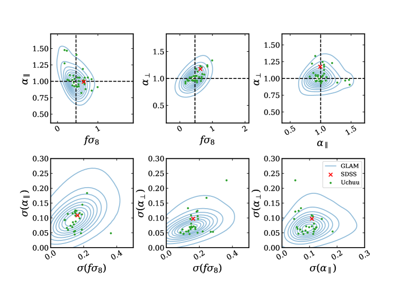
Figure 17: Upper row: Parameter values of $f\sigma_{8}$, $\alpha_{\parallel}$ and $\alpha_{\perp}$ measured from the GLAM-SDSSbao (blue contours), Uchuu-SDSSbao (green points), and SDSSbao light-cones (red cross). Dashed black lines represent the expected values for the fiducial cosmology. Lower row: The corresponding parameter errors.

The distribution of parameter values and their uncertainties can be seen in Fig. 17, where the results from the SDSSbao sample together with those from GLAM and Uchuu are shown in blue, orange and red respectively, and the black lines show the expected values of the parameters for the Planck fiducial cosmology. The results from GLAM- and Uchuu-SDSSbao are very consistent within each other and with the SDSSbao data, meaning that the mocks can be seen as a fair statistical representation of the data. We confirm that the fits we have performed are valid and have an acceptable $\chi^{2}/\mathrm{dof}$, for GLAM mocks being $\chi^{2}/\mathrm{dof}=1.00\pm 0.18$, for Uchuu mocks being $\chi^{2}/\mathrm{dof}=1.06\pm 0.18$ and for the SDSSbao sample being $\chi^{2}/\mathrm{dof}=0.99$.

Finally we use our best-fit values of the BAO-inferred $\alpha_{\parallel}$ and $\alpha_{\perp}$ parameters to provide a measurement of the Hubble distance and the (comoving) angular diameter distance at the effective redshift of the SDSSbao sample, i.e. $D_{\mathrm{H}}(z=0.15)/r_{d}=27.9^{+3.1}_{-2.7}$, $D_{\mathrm{M}}(z=0.15)/r_{d}=5.1^{+0.4}_{-0.4}$. These distance results are valuable since at present only the spherically averaged distance $D_{\mathrm{V}}(z=0.15)/r_{d}$ has been reported from BAO isotropic measurements from a similar SDSSbao sample by Ross et al. (2015), see below for our own BAO isotropic analysis.

5.4 Isotropic BAO measurements

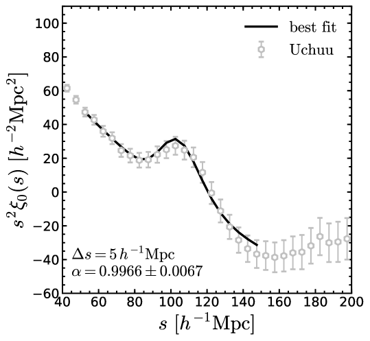
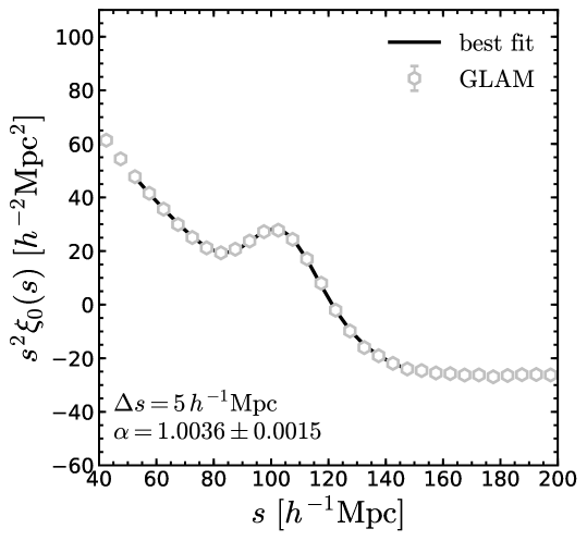
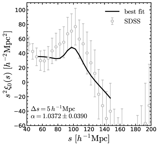
Figure 18: Measured (grey dots) and best-fit (solid black lines) correlation function monopole from the Uchuu (left panel) and GLAM (middle panel) simulated light-cones, and SDSS observations (right panel) at $z=0.15$ using a bin width of $\Delta s=5\,h^{-1}\rm{Mpc}$. The error bars for Uchuu and GLAM were rescaled by the square-root of the number of lightcones.

We also measure the isotropic BAO scale from our Uchuu-SDSSbao and the SDSSbao data at $z=0.15$. The BAO signal can clearly be seen in the correlation function monopole measured from both data set (see Fig. 16). The BAO scale can be extracted by fitting the monopole of the correlation function to a template that includes the dilation parameter, $\alpha$,

$$\alpha\equiv\frac{D_{\mathrm{V}}(z)r^{\mathrm{fid}}_{\mathrm{d}}}{D^{\mathrm{fid}}_{\mathrm{V}}(z)r_{\mathrm{d}}}\,,$$ (23)

where

$$D_{\mathrm{V}}(z)=\left[cz(1+z)^{2}D^{2}_{\mathrm{A}}(z)H^{-1}(z)\right]^{1/3}\,,$$ (24)

is the spherically average distance (Eisenstein et al., 2005); $\alpha$ is related to the anisotropic Alcock-Paczynski parameters $\alpha_{\perp}$ and $\alpha_{\parallel}$ given in eqs. 18 and 19, by $\alpha=\alpha_{\parallel}^{1/3}\alpha_{\perp}^{2/3}$.

To obtain the best-fit $\alpha$ value, we use Bayesian statistics and maximise the likelihood by adopting the BAO model of the monopole of the redshift-space correlation function as presented in Ross et al. (2015). We perform the fit to the simulations and data monopoles on scales $50<s<150~{}h^{-1}\mathrm{Mpc}$, using separation bins of width $\Delta s=5h^{-1}\mathrm{Mpc}$. The measured and the best-fit model of the correlation function monopole from the SDSSbao data and the simulated Uchuu and GLAM lightcones are shown in Fig. 18. We find $\alpha=0.9966\pm 0.0067$, $\alpha=1.0036\pm 0.0015$ and $\alpha=1.0372\pm 0.0390$ from Uchuu, GLAM, and the SDSSbao observations, respectively. Our best-fit $\alpha$ value for the SDSS data and its error is consistent with that reported by Ross et al. (2015), i.e. $\alpha=1.057\pm 0.037$.

From our dilation parameter estimate we measure a spherically averaged distance $D_{\mathrm{V}}(z=0.15)/r_{\mathrm{d}}=4.43\pm 0.16$, in agreement with the value $D_{\mathrm{V}}(z=0.15)/r_{\mathrm{d}}=4.47\pm 0.17$ measured by Ross et al. (2015). The values of $D_{\mathrm{V}}$ from the Uchuu and GLAM lightcone measurements are $D_{\mathrm{V}}(z=0.15)/r_{\mathrm{d}}=4.257\pm 0.028$ and $D_{\mathrm{V}}(z=0.15)/r_{\mathrm{d}}=4.304\pm 0.007$, respectively.

6 Summary

The cosmological interpretation of large galaxy surveys requires generation of high-fidelity simulated galaxy data. Here we describe and analyze publicly available Uchuu-SDSS lightcones: a set of simulated SDSS catalogues generated using the Uchuu $N$-body simulation. Uchuu is a large high-resolution cosmological simulation that follows the evolution of the dark matter across cosmic time in the Planck cosmology. The Uchuu-SDSS catalogues are tailored to reproduce the sky footprint and galaxy properties of the SDSS MGS observational sample. This facilitates the direct comparison between our simulated lightcones and the observational data to probe the Planck-$\Lambda$CDM cosmology model using the large-scale clustering signal.

The rest-frame $r$-band magnitudes, ${}^{0.1}M_{r}^{h}$, are assigned to the Uchuu haloes using the SHAM method, with a simple recipe for the scatter in the galaxy-halo connection. By construction, our scheme reproduces the SDSS and GAMA luminosity functions, and it reproduces to good accuracy the SDSS clustering (see Fig. 1), while using only one free parameter – the scatter. The resulting galaxy catalogues computed at different redshifts are combined in spherical shells and cut to the SDSS sky footprint. By placing observers at different positions in the cubic box, we produce a set of 8 independent Uchuu-SDSS lightcones, with only a small mutual overlap in volume. Additionally, an extended set of 32 lightcones, which overlap for $z>0.175$, are generated to increase the statistics for our SDSS RSD and BAO measurements. Galaxy colours are also produced using a Monte Carlo method that randomly draws colours from the ${}^{0.1}M_{r}^{h}$ and redshift-dependent $g-r$ distribution obtained from the GAMA survey. Redshifts, $r$-band magnitudes and $g-r$ colours are used to match each simulated galaxy to a galaxy in the SDSS sample. This allows us to assign absolute magnitudes, apparent magnitudes and $k$-corrections in the $u$, $g$, $i$ and $z$-bands in addition to stellar masses and specific star formation rates. Finally, we implement the effect of fibre collisions by applying a nearest neighbour correction to a set of galaxies situated in close angular proximity.

Our Uchuu-SDSS lightcones are able to recover the galaxy redshift distribution (see Fig. 5) and various galaxy properties from the SDSS survey to very high accuracy (see Figs. 6, 7 and 8). We also compute the galaxy correlation functions for several volume-limited samples corresponding to a wide range of luminosities (Fig. 9) and stellar mass cuts (Fig. 10), finding a very good agreement with the SDSS clustering down to the smallest $100\,h^{-1}\mathrm{kpc}$ scale. The colour- and stellar-mass-dependent galaxy clustering (see Fig. 11) is in general agreement with the SDSS results. Similarly, the simulated stellar mass function (Fig. 12) is in good agreement with that from SDSS data. We also provide the halo occupation distributions and parameters of the Uchuu-SDSS galaxies (Fig. 13), which are in agreement with previous SDSS analyses.

We explore the RSD and BAO signal in our Uchuu-SDSS lightcones and the SDSS data (see Fig. 16). In order to obtain high-precision covariance matrices for the error estimates of the RSD and BAO measurements, we create a large number of GLAM simulations. We apply HOD method to populate the GLAM halos with galaxies, generating a total of 5100 GLAM-SDSSbao lightcones. We measure $f\sigma_{8}$ and the anisotropic BAO parameters, $\alpha_{\perp}$ and $\alpha_{\parallel}$, from a full-shape model fit of the TPCF, finding a very good agreement between the SDSSbao data and our GLAM- and high-fidelity Uchuu-SDSSbao lighcones (see Fig. 17). Our results are given in Table 4. We obtain a $\gtrsim 30\%$ increase in precision on $f\sigma_{8}$, as compared to the previous measurement by (Howlett et al., 2015), which can be attributed to our better estimate of the covariance matrix.

We use our best-fit values of the BAO-inferred $\alpha_{\parallel}$ and $\alpha_{\perp}$ parameters to provide a measurement of the Hubble distance and the (comoving) angular diameter distance at the effective redshift of the SDSSbao sample, i.e. $D_{\mathrm{H}}(z=0.15)/r_{d}=27.9^{+3.1}_{-2.7}$, $D_{\mathrm{M}}(z=0.15)/r_{d}=5.1^{+0.4}_{-0.4}$. We highlight that these distance results are valuable since at present only the spherically averaged distance $D_{\mathrm{V}}(z=0.15)/r_{d}$ has been reported by Ross et al. (2015). Finally, we measure the isotropic dilation scale, $\alpha$, of the BAO signal by fitting a model template of the BAO peak (Ross et al., 2015), obtaining again a good agreement between the simulated and observational SDSS data (Fig. 18).

Based on our results, we conclude that the Planck CDM cosmology nicely explains the observed statistics of the large-scale structure of the SDSS main galaxy survey.

This work shows the great potential of the Uchuu simulation as a canvas for the creation of simulated galaxies (and quasars) for large surveys. The procedures presented in this paper can be readily applied for the creation of high-fidelity lightcones from Uchuu, and covariance errors from GLAM simulations, tailored for upcoming galaxy surveys such as DESI (DESI Collaboration et al., 2016), Euclid (Laureijs et al., 2011), and LSST (LSST Science Collaboration et al., 2009). This will aid the evaluation of analysis pipelines, the assessment of observational biases and systematic effects, and enable cosmological models to be probed.

Data Availability

The 32 Uchuu-SDSS galaxy lightcones, the 6 Uchuu-box galaxy catalogues at redshifts ${z=\{0,0.093,0.19,0.3,0.43,0.49\}}$, the 5100 Uchuu-SDSSbao galaxy lightcones, and the companion SDSS LSS catalogue used in this work are made available at http://www.skiesanduniverses.org/Simulations/Uchuu/, together With the information on how to read the data. For a list and brief description of the available catalogue columns, please see Appendix A.

Appendix A Content of the Uchuu-SDSS catalogues

Below is a list of the columns of each data set, along with a short description.

A.1 Uchuu-SDSS galaxy lightcones

Each Uchuu-SDSS lightcone has $\sim 590\,000$ galaxies in total (excluding the regions of low fibre-collision completeness), with the following columns:

• galaxy_type: indicates whether the galaxy is central or a satellite (0 for centrals, 1 for satellites).

• ra: right ascension (degrees).

• dec: declination (degrees).

• z_cos: cosmological redshift.

• z_obs: observed redshift (accounting for peculiar velocities).

• z_obs_fib: observed redshift including fibre collisions, i.e. fibre-collided galaxies get a nearest neighbour correction (see Section 3.3.5).

• k_corr_r: $r$-band $k$-correction at a reference redshift $z=0.1$. There are similar columns for the other SDSS photometric bands i.e. k_corr_u, k_corr_g, k_corr_i and k_corr_z.

• k_corr_r_fib: $r$-band $k$-correction, recomputed for fibre-collided galaxies using the nearest neighbour-corrected redshift, z_obs_fib.

• M_r: rest-frame $r$-band absolute magnitude ${}^{0.1}M_{r}^{h}$, $k$-corrected to $z=0.1$, with no E-correction. Similarly, the absolute magnitudes in the other bands are M_u, M_g, M_i and M_z.

• M_r_fib: $r$-band absolute magnitude accounting for fibre collisions, i.e. recomputed for fibre collided galaxies using the values of kcorr_r_fib and z_obs_fib.

• m_r: apparent $r$-band magnitude, $r$. The apparent magnitudes in the other bands are m_u, m_g, m_i and m_z.

• g_r: rest-frame $g-r$ colour $k$-corrected to $z=0.1$, ${}^{0.1}(g-r)$. This is the colour from our colour-assignment algorithm.

• g_r_obs: observer-frame $g-r$ colour, from our colour-assignment algorithm.

• stellar_mass_MPA: MPA stellar mass ($h^{-2}\mathrm{M_{\odot}}$).

• stellar_mass_granada_best: Granada best-fitting stellar mass ($h^{-2}\mathrm{M_{\odot}}$).

• stellar_mass_granada_median: Granada median stellar mass ($h^{-2}\mathrm{M_{\odot}}$).

• ssfr_MPA: MPA specific star formation rate ($\log_{10}(1/\mathrm{Gyr})$).

• ssfr_granada_best: Granada best-fitting stellar mass ($\log_{10}(1/\mathrm{Gyr})$).

• ssfr_granada_median: Granada median stellar mass ($\log_{10}(1/\mathrm{Gyr})$).

• idnn: ID of the nearest neighbour in the original catalogue (-1 if no galaxies are within $55^{\prime\prime}$; -2 if the galaxy is collided but keeps its true spectroscopic redshift).

• is_collided: indicates whether a galaxy is fibre-collided (is True if idnn is not either -1 or -2).

• completeness: fibre-collision completeness in the healpix pixel containing the galaxy.

• snap: snapshot number from the original Uchuu-box catalogue.

In addition, the following columns describe the DM host halo properties of the Uchuu-SDSS galaxies, taken from the original values in the Uchuu simulation halo catalogues.

• First_Acc_Scale: scale factor at which current and former satellites first passed through a larger halo.

• Macc: halo virial mass at accretion, excluding unbound particles ($h^{-1}\mathrm{M_{\odot}}$).

• Mvir_all: mass enclosed within the virial overdensity, including unbound particles ($h^{-1}\mathrm{M_{\odot}}$).

• Rvir: virial radius ($h^{-1}\mathrm{kpc}$).

• Vpeak: peak value of $V_{\mathrm{max}}$ over the halo history (physical $\mathrm{km}\text{\,}{\mathrm{s}}^{-1}$).

• halo_id: halo ID.

• halo_mass: mass enclosed within an overdensity of $200\rho_{\mathrm{crit}}$, where $\rho_{\mathrm{crit}}$ is the critical density at the snapshot redshift ($h^{-1}\mathrm{M_{\odot}}$).

• is_cen: indicates whether the halo is central (True for centrals, False for satellite).

• pid: ID of the parent central halo for satellite haloes, -1 for central haloes.

• pos: 3D position vector. The coordinate system of the Uchuu cubic box has been shifted so that the observer is at the origin, and there are periodic replications of the box (comoving $h^{-1}\mathrm{Mpc}$).

• rs: scale radius of a fitted NFW profile (comoving $h^{-1}\mathrm{kpc}$)

• vel: 3D velocity (physical $\mathrm{km\,s^{-1}}$).

• vrms: velocity dispersion (physical $\mathrm{km\,s^{-1}}$).

Additionally, a set of 10 random catalogues, each containing $10$ times the number of galaxies of an individual catalogue, are provided in order to facilitate the analysis of the simulated catalogues. The randoms are obtained by sampling galaxies randomly from the Uchuu-SDSS catalogues, but reassigning them a random sky position chosen with uniform probability within the footprint of the lightcone.

A.2 Uchuu-box galaxy catalogues

For the $(2~{}h^{-1}\mathrm{Gpc})^{3}$ Uchuu-box galaxy catalogues (at redshifts ${z=\{0,0.093,0.19\}}$), there are two galaxy properties: M_r and g_r, defined as in the previous subsection.

The halo columns are the same as in the Uchuu-SDSS lightcones, with a few exceptions: halo_id is renamed as id, and halo_mass is renamed as M200c. The columns pos, vel, and is_cen are removed, and the following are added:

• x: x-position of the halo/galaxy (comoving $\mathrm{Mpc}\text{\,}{\mathrm{\mathit{h}}}^{-1}$). Similarly for y and z.

• vx: x-velocity of the halo/galaxy (physical $\mathrm{km}\text{\,}{\mathrm{s}}^{-1}$). Similarly for vy and vz.

A.3 GLAM-SDSSbao galaxy lightcones

Our 5100 GLAM-SDSSbao lightcones, described in 5.1, have the following columns:

• galaxy_id: indicates whether the galaxy is central or a satellite (1 for centrals, 2 for satellites).

• ra: right ascension (degrees).

• dec: declination (degrees).

• z_cos: cosmological redshift.

• z_obs: observed redshift (accounting for peculiar velocities).

In addition, the following columns describe the DM host halo properties of the galaxies, taken from the original values found in the GLAM simulation halo catalogues,

• Mtotal: halo virial mass ($h^{-1}\mathrm{M_{\odot}}$).

• Rvir: halo virial radius ($h^{-1}\mathrm{kpc}$).

• rs: scale radius of a fitted NFW profile (comoving $h^{-1}\mathrm{kpc}$).

• pos: 3D position vector. The coordinate system of the GLAM cubic box has been shifted so that the observer is at the origin, and there are periodic replications of the box (comoving $h^{-1}\mathrm{Mpc}$).

• vel: 3D velocity (physical $\mathrm{km\,s^{-1}}$).

• vlos: velocity vector projected along line-of-sight, with the observer positioned at the origin ($\mathrm{km\,s^{-1}}$).

A.4 SDSS data sample

We also make available the observed SDSS galaxy sample, which consists of $497\,536$ (excluding regions of low fibre-collision completeness).The columns, which are defined the same way as in the Uchuu-SDSS lightcones (see A1), with the same units, are as follows:

• indx: ID of the galaxy.

• ra

• dec

• z: measured redshift, including fibre collisions.

• k_corr_r, k_corr_u, k_corr_g, k_corr_i, k_corr_z

• M_r, M_u, M_g, M_i, M_z

• m_r, m_u, m_g, m_i, m_z

• g_r

• g_r_obs

• mass_MPA

• mass_granada_best

• mass_granada_median

• ssfr_MPA

• ssfr_granada_best

• ssfr_granada_median

• idnn

• fgotten: fibre-collision completeness in the region containing the galaxy.

Additionally, a random file with $67$ times the number of galaxies of each GLAM-SDSSbao catalogue is made available to facilitate the analysis.

Appendix B The effect of scatter in SHAM

As discussed in Section 3.2, our SHAM model has only one free parameter $\sigma$, which roughly corresponds to the scatter in ${}^{0.1}M_{r}^{h}$ at a fixed value of our halo mass proxy, $V\mathrm{peak}$. In practice, the value of $\sigma$ affects mainly the amplitude of the TPCF for a given volume-limited sample, results are shown in Fig. 1 for different values of the scatter. Increasing the value of $\sigma$ introduces a larger number of low $V_{\mathrm{peak}}$ galaxies into the volume-limited samples, which are weakly clustered (and also removes high $V_{\mathrm{peak}}$ galaxies, which are strongly clustered). This has the effect of decreasing the amplitude of the TPCF. The effect of scatter is consequently larger for strongly clustered volume-limited samples, becoming negligible for samples with magnitude threshold ${}^{0.1}M_{r}^{h}>-20$. In order to tune the scatter parameter, we optimise the goodness-of-fit of the TPCF monopole for the Uchuu snapshot at $z=0.093$ to the SDSS measurements, finding an optimal value of $\sigma=0.5$. We choose this snapshot since it is the closest to the median SDSS redshift $z=0.1$. This value is in agreement with previous observational estimations of the scatter using SHAM. For example, Trujillo-Gomez et al. (2011) estimate the the scatter of ${}^{0.1}M_{r}^{h}$ at fixed halo circular velocity, by combining an estimate of the intrinsic scatter of the Tully-Fisher relation (Verheijen, 2001) with the scatter resulting from the distribution of dust extinction corrections in SDSS, arriving precisely at a value of $0.5$.

References

- Abazajian et al. (2009) Abazajian K. N., et al., 2009, ApJS, 182, 543
- Alam et al. (2021) Alam S., et al., 2021, Phys. Rev. D, 103, 083533
- Behroozi et al. (2013a) Behroozi P. S., Wechsler R. H., Wu H.-Y., 2013a, ApJ, 762, 109
- Behroozi et al. (2013b) Behroozi P. S., Wechsler R. H., Wu H.-Y., Busha M. T., Klypin A. A., Primack J. R., 2013b, ApJ, 763, 18
- Behroozi et al. (2019) Behroozi P., Wechsler R. H., Hearin A. P., Conroy C., 2019, MNRAS, 488, 3143
- Blanton (2006) Blanton M. R., 2006, ApJ, 648, 268
- Blanton et al. (2003a) Blanton M. R., et al., 2003a, AJ, 125, 2348
- Blanton et al. (2003b) Blanton M. R., et al., 2003b, ApJ, 592, 819
- Blanton et al. (2005) Blanton M. R., et al., 2005, AJ, 129, 2562
- Brinchmann et al. (2004) Brinchmann J., Charlot S., White S. D. M., Tremonti C., Kauffmann G., Heckman T., Brinkmann J., 2004, MNRAS, 351, 1151
- Brooks & Gelman (1998) Brooks S. P., Gelman A., 1998, Journal of Computational and Graphical Statistics, 7, 434
- Campbell et al. (2018) Campbell D., van den Bosch F. C., Padmanabhan N., Mao Y.-Y., Zentner A. R., Lange J. U., Jiang F., Villarreal A., 2018, MNRAS, 477, 359
- Chang et al. (2015) Chang Y.-Y., van der Wel A., da Cunha E., Rix H.-W., 2015, ApJS, 219, 8
- Charlot & Fall (2000) Charlot S., Fall S. M., 2000, ApJ, 539, 718
- Chaves-Montero et al. (2016) Chaves-Montero J., Angulo R. E., Schaye J., Schaller M., Crain R. A., Furlong M., Theuns T., 2016, MNRAS, 460, 3100
- Chen et al. (2020) Chen S.-F., Vlah Z., White M., 2020, J. Cosmology Astropart. Phys., 2020, 062
- Chen et al. (2021) Chen S.-F., Vlah Z., Castorina E., White M., 2021, J. Cosmology Astropart. Phys., 2021, 100
- Cole et al. (2005) Cole S., et al., 2005, MNRAS, 362, 505
- Colless et al. (2001) Colless M., et al., 2001, MNRAS, 328, 1039
- Conroy et al. (2006) Conroy C., Wechsler R. H., Kravtsov A. V., 2006, ApJ, 647, 201
- Conroy et al. (2009) Conroy C., Gunn J. E., White M., 2009, ApJ, 699, 486
- DESI Collaboration et al. (2016) DESI Collaboration et al., 2016, arXiv e-prints, p. arXiv:1611.00036
- Dembinski & et al. (2020) Dembinski H., et al. P. O., 2020, doi:10.5281/zenodo.3949207
- Duarte & Mamon (2015) Duarte M., Mamon G. A., 2015, MNRAS, 453, 3848
- Dubois et al. (2014) Dubois Y., et al., 2014, MNRAS, 444, 1453
- Eisenstein et al. (2005) Eisenstein D. J., et al., 2005, ApJ, 633, 560
- Feldman et al. (1994) Feldman H. A., Kaiser N., Peacock J. A., 1994, ApJ, 426, 23
- Foreman-Mackey et al. (2013) Foreman-Mackey D., Hogg D. W., Lang D., Goodman J., 2013, PASP, 125, 306
- Gao et al. (2005) Gao L., Springel V., White S. D. M., 2005, MNRAS, 363, L66
- Gelman & Rubin (1992) Gelman A., Rubin D. B., 1992, Statistical Science, 7, 457
- Gorski et al. (1999) Gorski K. M., Wandelt B. D., Hansen F. K., Hivon E., Banday A. J., 1999, arXiv e-prints, pp astro–ph/9905275
- Guo et al. (2015) Guo H., et al., 2015, MNRAS, 453, 4368
- Guzzo et al. (2008) Guzzo L., et al., 2008, Nature, 451, 541
- Hartlap et al. (2007) Hartlap J., Simon P., Schneider P., 2007, A&A, 464, 399
- Hayashi et al. (2003) Hayashi E., Navarro J. F., Taylor J. E., Stadel J., Quinn T., 2003, ApJ, 584, 541
- Howlett et al. (2015) Howlett C., Ross A. J., Samushia L., Percival W. J., Manera M., 2015, MNRAS, 449, 848
- Ishiyama et al. (2009) Ishiyama T., Fukushige T., Makino J., 2009, PASJ, 61, 1319
- Ishiyama et al. (2012) Ishiyama T., Nitadori K., Makino J., 2012, arXiv e-prints, p. arXiv:1211.4406
- Ishiyama et al. (2021) Ishiyama T., et al., 2021, MNRAS,
- Ivezić et al. (2019) Ivezić Ž., et al., 2019, ApJ, 873, 111
- Kaiser (1987) Kaiser N., 1987, MNRAS, 227, 1
- Kauffmann et al. (2003) Kauffmann G., et al., 2003, MNRAS, 341, 33
- Kennicutt (1998) Kennicutt Robert C. J., 1998, ARA&A, 36, 189
- Klypin & Holtzman (1997) Klypin A., Holtzman J., 1997, arXiv e-prints, pp astro–ph/9712217
- Klypin & Prada (2018) Klypin A., Prada F., 2018, MNRAS, 478, 4602
- Kravtsov et al. (2004) Kravtsov A. V., Berlind A. A., Wechsler R. H., Klypin A. A., Gottlöber S., Allgood B., Primack J. R., 2004, ApJ, 609, 35
- Kroupa (2001) Kroupa P., 2001, MNRAS, 322, 231
- LSST Science Collaboration et al. (2009) LSST Science Collaboration et al., 2009, arXiv e-prints, p. arXiv:0912.0201
- Laureijs et al. (2011) Laureijs R., et al., 2011, arXiv e-prints, p. arXiv:1110.3193
- Leslie et al. (2016) Leslie S. K., Kewley L. J., Sanders D. B., Lee N., 2016, MNRAS, 455, L82
- Lin et al. (2020) Lin S., et al., 2020, MNRAS, 498, 5251
- Loveday et al. (2012) Loveday J., et al., 2012, MNRAS, 420, 1239
- Marinoni & Hudson (2002) Marinoni C., Hudson M. J., 2002, ApJ, 569, 101
- McCullagh et al. (2017) McCullagh N., Norberg P., Cole S., Gonzalez-Perez V., Baugh C., Helly J., 2017, arXiv e-prints, p. arXiv:1705.01988
- Moustakas et al. (2013) Moustakas J., et al., 2013, ApJ, 767, 50
- Peebles (1980) Peebles P. J. E., 1980, The large-scale structure of the universe
- Perlmutter et al. (1999) Perlmutter S., et al., 1999, ApJ, 517, 565
- Pillepich et al. (2018) Pillepich A., et al., 2018, MNRAS, 475, 648
- Planck Collaboration et al. (2016) Planck Collaboration et al., 2016, A&A, 594, A13
- Planck Collaboration et al. (2020) Planck Collaboration et al., 2020, A&A, 641, A6
- Reddick et al. (2013) Reddick R. M., Wechsler R. H., Tinker J. L., Behroozi P. S., 2013, ApJ, 771, 30
- Riess et al. (1998) Riess A. G., et al., 1998, AJ, 116, 1009
- Rodríguez-Torres et al. (2016) Rodríguez-Torres S. A., et al., 2016, MNRAS, 460, 1173
- Ross et al. (2015) Ross A. J., Samushia L., Howlett C., Percival W. J., Burden A., Manera M., 2015, MNRAS, 449, 835
- Safonova et al. (2021) Safonova S., Norberg P., Cole S., 2021, MNRAS, 505, 325
- Salim et al. (2007) Salim S., et al., 2007, ApJS, 173, 267
- Schaye et al. (2015) Schaye J., et al., 2015, MNRAS, 446, 521
- Seljak & McDonald (2011) Seljak U., McDonald P., 2011, Journal of Cosmology and Astroparticle Physics, 2011, 039
- Shu et al. (2012) Shu Y., Bolton A. S., Schlegel D. J., Dawson K. S., Wake D. A., Brownstein J. R., Brinkmann J., Weaver B. A., 2012, AJ, 143, 90
- Skibba & Sheth (2009) Skibba R. A., Sheth R. K., 2009, MNRAS, 392, 1080
- Smith et al. (2017) Smith A., Cole S., Baugh C., Zheng Z., Angulo R., Norberg P., Zehavi I., 2017, MNRAS, 470, 4646
- Smith et al. (2019) Smith A., et al., 2019, MNRAS, 484, 1285
- Smith et al. (2022a) Smith A., Cole S., Grove C., Norberg P., Zarrouk P., 2022a, arXiv e-prints, p. arXiv:2206.08763
- Smith et al. (2022b) Smith A., Cole S., Grove C., Norberg P., Zarrouk P., 2022b, arXiv e-prints, p. arXiv:2207.04902
- Springel et al. (2018) Springel V., et al., 2018, MNRAS, 475, 676
- Stiskalek et al. (2021) Stiskalek R., Desmond H., Holvey T., Jones M. G., 2021, MNRAS, 506, 3205
- Swanson et al. (2008) Swanson M. E. C., Tegmark M., Hamilton A. J. S., Hill J. C., 2008, MNRAS, 387, 1391
- Szewciw et al. (2022) Szewciw A. O., Beltz-Mohrmann G. D., Berlind A. A., Sinha M., 2022, ApJ, 926, 15
- Takada et al. (2014) Takada M., et al., 2014, PASJ, 66, R1
- Taruya et al. (2010) Taruya A., Nishimichi T., Saito S., 2010, Phys. Rev. D, 82, 063522
- Taylor et al. (2011) Taylor E. N., et al., 2011, MNRAS, 418, 1587
- Trujillo-Gomez et al. (2011) Trujillo-Gomez S., Klypin A., Primack J., Romanowsky A. J., 2011, ApJ, 742, 16
- Vale & Ostriker (2004) Vale A., Ostriker J. P., 2004, MNRAS, 353, 189
- Verheijen (2001) Verheijen M. A. W., 2001, ApJ, 563, 694
- Wechsler (2001) Wechsler R. H., 2001, PhD thesis, UNIVERSITY OF CALIFORNIA, SANTA CRUZ
- Wechsler & Tinker (2018) Wechsler R. H., Tinker J. L., 2018, ARA&A, 56, 435
- Wechsler et al. (2006) Wechsler R. H., Zentner A. R., Bullock J. S., Kravtsov A. V., Allgood B., 2006, ApJ, 652, 71
- White et al. (2014) White M., Tinker J. L., McBride C. K., 2014, MNRAS, 437, 2594
- York et al. (2000) York D. G., et al., 2000, AJ, 120, 1579
- Zehavi et al. (2005) Zehavi I., et al., 2005, ApJ, 630, 1
- Zehavi et al. (2011) Zehavi I., et al., 2011, ApJ, 736, 59
- Zhao et al. (2021) Zhao C., et al., 2021, MNRAS, 503, 1149
- de la Torre et al. (2013) de la Torre S., et al., 2013, A&A, 557, A54