Non-equilibrium attractor in high-temperature QCD plasmas

Abstract

We establish the existence of a far-from-equilibrium attractor in weakly-coupled gauge theory undergoing 0+1d Bjorken expansion which goes beyond the energy-momentum tensor to the detailed form of the one-particle distribution function. We then demonsrate that the dynamics can be rescaled at intermediate times and represented by universal exponents. Finally, we assess different procedures for reconstructing the full one-particle distribution function from the energy-momentum tensor along the attractor and discuss implications for the freeze-out procedure used in the phenomenological analysis of ultra-relativistic nuclear collisions

1 Introduction

In the precision era of heavy ion collisions there has been an increased interest in understanding and quantifying the effects of non-equilibrium corrections present at different stages in heavy ion collisions. Non-equilibrium corrections are significantly present and particularly important in two main phases of the dynamical evolution: (I) pre-hydrodynamics (pre-equilibrium), and (II) freeze out (particlization). Non-equilibrium attractors can be used to explore the approach to equilibrium and have been widely applied to examine the applicability of hydrodynamic theories out-of-equilibrium in many approaches. In this work [1], we employ a microscopic approach based on quantum chromodynamics (QCD) effective kinetic theory (EKT), which is derived using weak-coupling methods. The method is applicable at high temperatures and is appropriate for modelling the initial stages of ultrarelativistic heavy-ion collisions. In parametrically isotropic systems, EKT [2, 3] gives a leading-order accurate description (in $\alpha_{s}$) of the time evolution of the one-particle distribution function in QCD and allows for a numerical realization of the so-called bottom-up thermalization scenario [5]. The description is based on the relativistic Boltzmann equation

$$-\frac{df(\mathbf{p})}{d\tau}+\frac{p_{z}}{\tau}\partial_{p_{z}}f=\mathcal{C}_{1\leftrightarrow 2}[f(\mathbf{p})]+\mathcal{C}_{2\leftrightarrow 2}[f(\mathbf{p})]\,,$$ (1)

where $f(\mathbf{p})$ is the gluonic one-particle distribution function (per degree of freedom). The elastic scattering term $\mathcal{C}_{2\leftrightarrow 2}$ and the effective inelastic term $\mathcal{C}_{1\leftrightarrow 2}$ include physics of dynamical screening and Landau-Pomeranchuck-Migdal suppression. For the numerical solution of Eq. (1), we discretize $n(\mathbf{p})=p^{2}f(\mathbf{p})$ on an optimized momentum-space grid and use Monte Carlo sampling to compute the integrals appearing in the elastic and inelastic collisional kernels. The algorithm used is based on Refs. [3, 4, 6, 7].

2 Non-equilibrium QCD attractor for higher moments

The time evolution of integral moments which characterize the momentum dependence of the distribution function is given by  [8]

$${\cal M}^{nm}(\tau)\equiv\int\frac{d^{3}p}{(2\pi)^{3}}\,p^{n-1}\,p_{z}^{2m}\,f(\tau,\mathbf{p})\,,$$ (2)

where $p=|{\bf p}|$. Note that the energy density is given by $\varepsilon=\nu{\cal M}^{20}$, longitudinal pressure by $P_{L}=\nu{\cal M}^{01}$, and number density by $n=\nu{\cal M}^{10}$ for $\nu$ degrees of freedom ($\nu=2d_{A}$ for $d_{A}$ adjoint degrees of freedom). These moments will be scaled by their corresponding equilibrium values with $\overline{\cal{M}}^{nm}(\tau)\equiv{\cal M}^{nm}(\tau)/{\cal M}^{nm}_{\rm eq}(\tau)$, where, using a Bose distribution, one obtains

$${\cal M}^{nm}_{\rm eq}=\frac{T^{n+2m+2}\Gamma(n+2m+2)\zeta(n+2m+2)}{2\pi^{2}(2m+1)}\,.$$ (3)

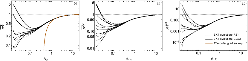
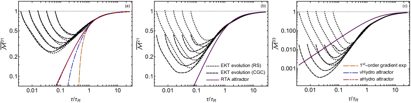
Figure 1: Evolution of the scaled moments (a) $\overline{\cal{M}}^{01}$, (b) $\overline{\cal{M}}^{21}$, and (c) $\overline{\cal{M}}^{33}$. The top row corresponds to varying the initial anisotropy ($\xi_{0}$) and bottom row to varying the initialization time $\tau_{0}$. Black dotted and dashed lines show the EKT evolution with RS and CGC initial conditions, respectively. The purple solid line is the exact RTA attractor, the orange long-dashed line is the first-order gradient expansion result, the blue dot-dashed line is the DNMR vHydro attractor, and the red dot-dot-dashed line is the aHydro attractor.

The temperature $T$ here corresponds to the temperature of an equilibrium system with the same energy density, given by $T=(30\varepsilon/\nu\pi^{2})^{1/4}$.

These simulations are initialized with either of the two following initial conditions: (1) spheroidally-deformed thermal initial conditions which we will refer to as “RS” initial conditions [9]

$$f_{0,{\rm RS}}(\mathbf{p})=f_{\rm Bose}\!\left(\sqrt{\mathbf{p}^{2}+\xi_{0}p_{z}^{2}}/\Lambda_{0}\right),$$ (4)

where $-1<\xi_{0}<\infty$ encodes the initial momentum-anisotropy and $\Lambda_{0}$ is a temperature-like scale which sets the magnitude of the initial average transverse momentum, or (2) non-thermal color-glass-condensate (CGC) inspired initial conditions [4]

$$f_{0,\rm CGC}(\mathbf{p}) = \frac{2A}{\lambda}\frac{\tilde{\Lambda}_{0}}{\sqrt{\mathbf{p}^{2}+\xi_{0}p_{z}^{2}}}e^{-\frac{2}{3}\left(\mathbf{p}^{2}+\xi_{0}\hat{p}_{z}^{2}\right)/\tilde{\Lambda}_{0}^{2}}\,.$$ (5)

In Fig. 1, we present results for the evolution of three scaled moments, $\overline{\cal{M}}^{01}$, $\overline{\cal{M}}^{21}$, and $\overline{\cal{M}}^{33}$, in panels (a), (b), and (c), respectively. In the top panel, we fix the initialisation time and examine the existence of the forward attractor or the convergence toward late time equilibrium state of the system. In the bottom panel which corresponds to the “pullback” attractor or the convergence to the free streaming phase of the dynamics, we vary the initialization time toward asymptotically early times $\tau\sim 0$. As we show in Fig. (1), different solutions to Eq. (1) collapse to a universal curve at roughly $\tau/\tau_{R}\sim 0.5$ which indicates insensitivity to initial anisotropy and occupancy and confirms the existence of an attractor solution [1].

2.1 Re-scaling the turning point

In addition to looking for scaling properties at early and late times [10, 11], one can then also investigate whether there is universal scaling dynamics in the initialization time $\omega_{0}=\tau_{0}/\tau_{R}$ at the turning point. With $\omega\equiv\tau/\tau_{R}$, we define the latter as the time $\omega_{nm}(\omega_{0})$ of the minimum of the moment $\overline{\mathcal{M}}^{nm}(\omega_{0})$, assuming that both $\omega_{nm}$ and $\overline{\mathcal{M}}^{nm}$ are power laws in $\omega_{0}$ with $\overline{\mathcal{M}}^{nm}\sim\omega_{0}^{A_{nm}}$ and $\omega_{nm}\sim\omega_{0}^{B_{nm}}$. If we also assume that the scaling exponents for fixed $n,m$ are universal and independent of the initial conditions, we can estimate their value by taking the average of the exponents from the fits to the RS and CGC initial conditions. Then, taking both $A_{nm}$ and $B_{nm}$ to depend linearly on $n$ and $m$, the resulting fits are

$$A_{nm} =-0.0604726\,(2-n)+0.340507\,m\,,$$ (6)

$$B_{nm} =0.51845-0.0285393\,n+0.0452043\,m\,.$$ (7)

Interestingly, we note that the exponent $B_{nm}$ seems to be approximately $1/2$ with small corrections for different $n,m$ while the exponent $A_{nm}$ shows strong dependence on $m$ and depends on $n$ only weakly [12] (see Fig. (2)).

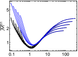
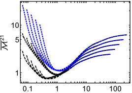
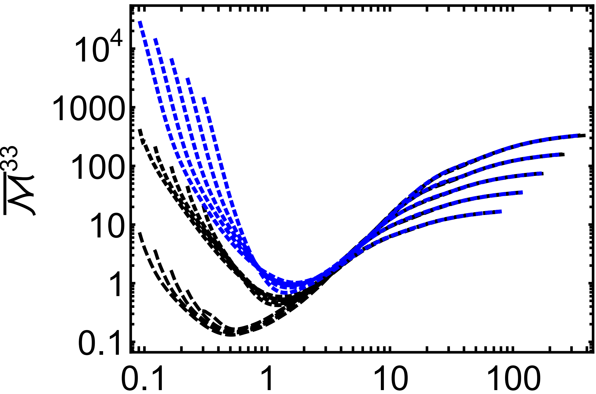
Figure 2: Rescaled moments $\overline{\mathcal{M}}^{nm}/\omega_{0}^{A_{nm}}$ as functions of $\omega/\omega_{0}^{B_{nm}}$ for different sets of initial conditions and initialization times $\omega_{0}=\tau_{0}/\tau_{R}$. Rescaling a particular moment and the scaled time $\omega$ reproduces a universal rescaling at the turning point at which the microscopic interactions begin to take over the dynamics.

3 Reconstructing the one-particle distribution function from $T^{\mu\nu}$

While the fluid-dynamic theories do not specify the higher moments of the distribution functions, in phenomenological applications it is a common practice to infer the full shape of the distribution from the shear components of the energy-momentum tensor only for use in freeze out. For a given $T^{\mu\nu}$, the linearized viscous correction to the one-particle distribution function, $\delta f$ can be locally computed given an assumption of the collision kernel. Herein, we consider two possible forms for $\delta f$. The (i) quadratic ansatz

$$\frac{\delta f_{(i)}}{f_{\rm eq}(1+f_{\rm eq})}=\frac{3\overline{\Pi}}{16T^{2}}(p^{2}-3p_{z}^{2})\,,$$ (8)

which results from a wide set of models. Here $\overline{\Pi}=\Pi/\epsilon=1/3-T^{zz}/\epsilon$. At full leading-order, however, QCD EKT has a more rich structure; for large $p\gg T$, QCD EKT reduces to power law form of the (ii) Landau-Pomeranchuck-Migdal (LPM) ansatz

$$\frac{\delta f_{(ii)}}{f_{\rm eq}(1+f_{\rm eq})}=\frac{16\overline{\Pi}}{21\sqrt{\pi}\,T^{3/2}}\!\left(p^{3/2}-\frac{3p_{z}^{2}}{\sqrt{p}}\right).$$ (9)

This $p^{1.5}$ power-law is numerically close to $\propto p^{1.38}$, which was found to describe the high-momentum region of the full EKT result [13]. Finally, we consider the non-linear (iii) aHydro freeze-out ansatz in which one assumes that the distribution function can be approximated by a spheroidally-deformed Bose-distribution $f(p)=f_{\rm Bose}(\sqrt{{\bf p}^{2}+\xi p_{z}^{2}}/\Lambda)$ [9, 14, 15].

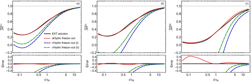
Figure 3: Evolution of the scaled moments (a) $\overline{\cal{M}}^{11}$, (b) $\overline{\cal{M}}^{21}$, and (c) $\overline{\cal{M}}^{22}$. The black solid line is a typical EKT evolution, the red-dashed line is the $P_{L}$-matched aHydro result for a given moment, the blue and green dot-dashed lines are the corresponding vHydro results using , respectively. The relative error shown in the bottom panels is (${\rm approximation}/{\rm EKT}-1$).

The different moments obtained by the above prescriptions are compared to the EKT attractor solution in Fig. 3. At late times $\tau>5\,\tau_{R}$, the low-order moments are described within a few percent by all the prescriptions, while some discrepancy remains even at $\tau\sim 20\,\tau_{R}$ between the quadratic ansatz (i) and our EKT results. The agreement worsens at earlier times and, around $\tau\sim\tau_{R}$ where the corrections to longitudinal pressure start to become sizable $P_{L}/P_{L}^{\rm eq}\sim 65\%$, ${\cal M}^{11}$ exhibits an approximately $20\%$ disagreement between EKT and both linearized ansatze. The disagreement increases for higher moments and at earlier times. In contrast, we observe good agreement between the aHydro ansatz and our EKT results at all times. As a result, when considering higher-moments or applying early-time freeze-out for smaller systems such as peripheral nucleus-nucleus collisions and proton-nucleus collision, the aHydro freeze-out ansatz is favored.

Acknowledgements: M.S. and D.A. were supported by the U.S. Department of Energy, Office of Science, Office of Nuclear Physics Award No. DE-SC0013470. D.A. is also supported by the US-DOE Nuclear Science Grant No. DE-SC0020633. K.B. is supported in part by the Austrian Science Fund (FWF) project P 34455. The authors wish to acknowledge the Ohio Supercomputer Center project No. PGS0251 and the Vienna Scientific Cluster (VSC) project 71444 for computational resources.

References

- [1] D. Almaalol, A. Kurkela, and M. Strickland, Phys. Rev. Lett. 125 (2020).
- [2] P. Arnold, G. Moore, and L. Yaffe, JHEP 01, 0209353 (2003).
- [3] Y. Abraao, C. Mark, A. Kurkela, E. Lu, and G.D. Moore, Physical Review D. 89, 074036 (2014).
- [4] A. Kurkela and Y. Zhu, Phys. Rev. Lett. 115, 182301 (2015).
- [5] R. Baier, A.H. Mueller, D. Schiff, and D.T. Son, Phys. Lett. B105, 0009237 (2001).
- [6] L. Keegan, A. Kurkela, P. Romatschke, W. van der Schee, and Y. Zhu, JHEP 04, 031 (2016).
- [7] P. Arnold, G.D. Moore, and L. Yaffe, JHEP 05, 051 (2003).
- [8] M. Strickland, JHEP 12, 128 (2018).
- [9] P. Romatschke and M. Strickland, Phys. Rev. D68, 036004 (2003).
- [10] A. Kurkela, W. van der Schee, U.A. Wiedemann, and B. Wu, Phys. Rev. Lett. 124 (2020).
- [11] X. Du, M.P. Heller, S. Schlichting, and V. Svensson, Phys. Rev. D 106 014016 (2022).
- [12] D. Almaalol and K. Boguslavski, forthcoming.
- [13] K. Dusling, G.D. Moore, and D. Teaney, Phys. Rev. C81, 034907 (2010).
- [14] W. Florkowski and R. Ryblewski, Phys. Rev. C83, 034907 (2011).
- [15] M. Martinez and M. Strickland, Nucl. Phys. A848 (2010).