Geodesics on an arbitrary ellipsoid of revolution

Abstract

The algorithms given in Karney, J. Geodesy 87, 43–55 (2013), to compute geodesics on terrestrial ellipsoids are extended to apply to ellipsoids of revolution with arbitrary eccentricity. For the direct and inverse geodesic problems, this entails implementing the formulation in terms of elliptic integrals given by Legendre and Cayley. The integral for the area of geodesic polygons is computed in terms of the discrete sine transform of the integrand. In all cases, accuracy close to full machine precision is achieved. An open-source implementation of these algorithms is available.

List of symbols

$a$	equatorial radius of the ellipsoid
$b$	its polar semi-axis
$f$	$(a-b)/a$, the flattening
$n$	$(a-b)/(a+b)$, the third flattening
$e$	$\sqrt{a^{2}-b^{2}}/a$, the eccentricity
$e^{\prime}$	$\sqrt{a^{2}-b^{2}}/b$, the second eccentricity
$\phi$	geographic latitude, north positive
$\lambda$	longitude, east positive
$\alpha$	azimuth of the geodesic, clockwise from north
$\alpha_{0}$	azimuth at the node
$s$	distance along the geodesic
$\beta$	parametric latitude; $a\tan\beta=b\tan\phi$
$\omega$	longitude on the auxiliary sphere
$\sigma$	arc length on the auxiliary sphere
$c$	the authalic radius
$S$	the area between the geodesic and the equator

The quantities $s$, $\sigma$, $\lambda$, and $\omega$ are measured from the node, the point where the geodesic crosses the equator in the northward direction. A single subscript refers to a specific point, e.g., $s_{1}$ measures the distance from the node to point $1$; for $s$, $\sigma$, and $\lambda$, a double subscript denotes a difference, e.g., $\lambda_{12}=\lambda_{2}-\lambda_{1}$.

1 Introduction

In an earlier paper, Algorithms for geodesics (Karney, 2013, henceforth referred to as AG), I presented algorithms for solving geodesic problems on an ellipsoid of revolution. This built on the classic work of Bessel (1825) and Helmert (1880) to give full double precision accuracy for ellipsoids with flattening satisfying $\lvert f\rvert\leq\frac{1}{100}$. A small improvement, described in Appendix A.2, extended this range $\lvert f\rvert\leq\frac{1}{50}$. Perhaps the most consequential innovation of AG was the reliable solution of the inverse geodesic problem, computing the shortest path between two arbitrary points on the ellipsoid. (Previously, the state of the art was provided by Vincenty (1975), which sometimes fails to converge.) Another important advance was turning the formulation of Danielsen (1989) for the area between a geodesic segment and the equator into an algorithm for computing accurately the area of any geodesic polygon, a polygon whose edges are geodesics. These algorithms allow geodesic problems to be reliably solved and this, in turn, has meant that they have been widely adopted in a variety of disciplines.

The present paper seeks to extend the treatment to arbitrary ellipsoid (in this paper, the term “ellipsoid” should be understood to mean “ellipsoid of revolution”). The condition $\lvert f\rvert\leq\frac{1}{50}$ covers all terrestrial applications. However, for the giant planets in our solar system, $f$ lies outside this range (for Saturn, we have $f\approx\frac{1}{10}$). For geodesic calculations, the solutions of the direct and inverse problems, this is a matter of realizing the formulation in terms of elliptic integrals, originally given by Legendre, as a usable algorithm. Generalizing the computation of the area of a geodesic polygon required a novel approach using the discrete sine transform.

Although the mathematical techniques used in this paper might be daunting for some readers, the concepts of geodesics with their interlocking definitions in terms of straightest lines and shortest paths are readily grasped. Furthermore, geodesics have well understood properties, for example:

• the shortest path from a point to a line intersects the line at right angles;

• shortest geodesics satisfy the triangle inequality and the other conditions that define a metric space;

• consequently, nearest neighbor problems can be solved efficiently using a vantage-point tree (Uhlmann, 1991; Yianilos, 1993).

It’s therefore possible, indeed it might be preferable, to tackle many problems involving geodesics by treating the implementation described here as a reliable “black box”.

The appendices cover various small improvements in the original algorithms given in AG and compare the algorithms presented here with recent work by Nowak and Nowak Da Costa (2022).

2 Geodesics in terms of elliptic integrals

2.1 Formulation of Legendre and Cayley

One of the earliest systematic studies of geodesics on an ellipsoid was given by Legendre (1811, §§126–129) who cast the solution in terms of his elliptic integrals. However, when Bessel later wished to obtain numerical results for the course of a geodesic, he stated “Because the tools to compute these special functions [elliptic integrals] are not yet sufficiently versatile, we instead develop a series solution which converges rapidly because $e^{2}$ is so small.” Bessel’s approach, series expansions valid for small flattening, became the mainstay for solving the geodesic problem. For a long time, elliptic integrals continued to be difficult to compute conveniently; for example, Abramowitz and Stegun (1964, Chap. 19) only provides tables for the elliptic integrals for selected values of the modulus and parameter. This obstacle was only removed with the work of Carlson (1995) as we describe below.

Before we give Legendre’s solution, let us review the formulation in terms of the auxiliary sphere; see Fig. 2 of AG. This is a construct used implicitly by Legendre and explicitly by Bessel that maps the path of the geodesic on the ellipsoid onto a great circle on the sphere. The latitude $\phi$ is mapped to the parametric latitude $\beta$, the azimuth $\alpha$ is preserved, and $\lambda$ and $s$ are related to the corresponding spherical variables $\omega$ and $\sigma$ by (Karney, 2011, Appendix A)

$$\frac{1}{a}\frac{\mathrm{d}s}{\mathrm{d}\sigma}=\frac{\mathrm{d}\lambda}{\mathrm{d}\omega}=\sqrt{1-e^{2}\cos^{2}\beta}.$$ (1)

Substituting the results from spherical trigonometry,

$$\frac{\mathrm{d}\omega}{\mathrm{d}\sigma} =\frac{\sin\alpha}{\cos\beta}=\frac{\sin\alpha_{0}}{\cos^{2}\beta},$$ (2)

$$\sin\beta =\cos\alpha_{0}\sin\sigma,$$ (3)

we obtain

$$\frac{s}{b} =\int_{0}^{\sigma}\sqrt{1+k^{2}\sin^{2}\sigma^{\prime}}\,\mathrm{d}\sigma^{\prime},$$ (4)

$$\lambda =(1-f)\sin\alpha_{0}\int_{0}^{\sigma}\frac{\sqrt{1+k^{2}\sin^{2}\sigma^{\prime}}}{1-\cos^{2}\alpha_{0}\sin^{2}\sigma^{\prime}}\,\mathrm{d}\sigma^{\prime},$$ (5)

$$J(\sigma) =\int_{0}^{\sigma}\frac{k^{2}\sin^{2}\sigma^{\prime}}{\sqrt{1+k^{2}\sin^{2}\sigma^{\prime}}}\,\mathrm{d}\sigma^{\prime},$$ (6)

where $k=e^{\prime}\cos\alpha_{0}$. $J(\sigma)$ is a term appearing in the expressions for the reduced length $m$ and the geodesic scale $M$; both these quantities, which were introduced by Gauss (1828), describe the behavior of nearby geodesics; see Sec. 3 of AG. These expressions can be put in the form of Legendre’s elliptic integrals,

$$\frac{s}{b} =E(\sigma,ik),$$ (7)

$$\lambda =(1-f)\sin\alpha_{0}G(\sigma,\cos^{2}\alpha_{0},ik),$$ (8)

$$J(\sigma) =E(\sigma,ik)-F(\sigma,ik),$$ (9)

where

$$G(\phi,\alpha^{2},k) =\int_{0}^{\phi}\frac{\sqrt{1-k^{2}\sin^{2}\theta}}{1-\alpha^{2}\sin^{2}\theta}\,\mathrm{d}\theta$$

$$=\frac{k^{2}}{\alpha^{2}}F(\phi,k)+\biggl{(}1-\frac{k^{2}}{\alpha^{2}}\biggr{)}\Pi(\phi,\alpha^{2},k),$$ (10)

and $F(\phi,k)$, $E(\phi,k)$, and $\Pi(\phi,\alpha^{2},k)$, are incomplete elliptic integrals (Olver et al., 2010, §http://dlmf.nist.gov/19.2.ii). Equations (7) and (8) are similar to the expressions given by Legendre; the only significant difference is that our formulas involve an imaginary modulus, $ik$, because we choose our origin for geodesics, $\sigma=0$, to be at the node (rather than at the vertex which was Legendre’s choice). This is inconsequential because the definitions of the elliptic integrals involve the square of the modulus; furthermore, for prolate ellipsoids, $ik$ is real.

Equations (5) and (8) for $\lambda$ are inconvenient to use in practice because the integrands are arbitrarily large as the geodesic passes close to a pole leading to a nearly discontinuous change in $\lambda$. Of course, this is the behavior of great circles as they approach a pole, and it is easily described by spherical trigonometry. It is therefore advantageous to split the expression for $\lambda$ into two terms, one involving $\omega$ to describe the basic behavior plus another, proportional to $f$ and involving special functions, to describe the ellipsoidal correction. This can be achieved by integrating

$$\frac{\mathrm{d}(\lambda-\omega)}{\mathrm{d}\omega}=\sqrt{1-e^{2}\cos^{2}\beta}-1,$$ (11)

which gives

$$\lambda=\omega-e^{2}\sin\alpha_{0}\int_{0}^{\sigma}\frac{1}{1+(1-f)\sqrt{1+k^{2}\sin^{2}\sigma^{\prime}}}\,\mathrm{d}\sigma^{\prime},$$ (12)

where the near-singular behavior of $\lambda$ is captured by $\omega$ with the difference given by a well behaved integral. This is the starting point for Bessel’s series solution.

Cayley (1870) found a similar way to transform Eq. (8) to give

$$\lambda=\chi-\frac{e^{\prime 2}}{\sqrt{1+e^{\prime 2}}}\sin\alpha_{0}H(\sigma,-e^{\prime 2},ik),$$ (13)

where

$$\tan\chi =\sqrt{\frac{1+e^{\prime 2}}{1+k^{2}\sin^{2}\sigma}}\tan\omega,$$ (14)

$$H(\phi,\alpha^{2},k) =\int_{0}^{\phi}\frac{\cos^{2}\theta}{(1-\alpha^{2}\sin^{2}\theta)\sqrt{1-k^{2}\sin^{2}\theta}}\,\mathrm{d}\theta$$

$$=\frac{1}{\alpha^{2}}F(\phi,k)+\biggl{(}1-\frac{1}{\alpha^{2}}\biggr{)}\Pi(\phi,\alpha^{2},k).$$ (15)

Now the main contribution to $\lambda$ is $\chi$, a variable that behaves similarly to the longitude near a pole, and the elliptic integral is relegated to a correction term; not only is it multiplied by $e^{\prime 2}$ but the parameter of the elliptic integral, $-e^{\prime 2}$ is also small. This allows the longitude to be computed more accurately. The equivalence of the two expressions for $\lambda$, Eqs. (8) and (13), follows from Olver et al. (2010, Eq. http://dlmf.nist.gov/19.7.E8).

2.2 Numerical evaluation of the elliptic integrals

Carlson (1995) provided high quality algorithms that allowed symmetric elliptic integrals (Olver et al., 2010, §http://dlmf.nist.gov/19.16) to be computed to arbitrary accuracy. Legendre’s elliptic integrals can then be simply evaluated using Olver et al. (2010, §http://dlmf.nist.gov/19.25.i). In our implementation, we also use the amendments to Carlson’s paper given in Olver et al. (2010, §http://dlmf.nist.gov/19.36.i).

With these methods in hand, we review the solutions of the direct and inverse geodetic problems. We first discuss the direct problem, determining the final position $\phi_{2}$, $\lambda_{2}$ and azimuth $\alpha_{2}$, given a starting position $\phi_{1}$, $\lambda_{1}$, initial azimuth $\alpha_{1}$, and distance $s_{12}$. The starting information allows us to calculate the parameter characterizing the geodesic, $\alpha_{0}$. Equations (7) and (13) above provide a reliable way to follow a geodesic arbitrarily far given its starting position and initial azimuth. The independent parameter in these equations is $\sigma$. Because we are given the distance $s_{12}$ to the second point, we need to invert Eq. (7) to find $\sigma$ in terms of $s$. This presents no difficulty; $s$ is a monotonically increasing function of $\sigma$ so there’s a unique solution and, provided we’re sufficiently close to the solution, Newton’s method can be used to obtain an accurate result; the derivative needed for Newton’s method, $\mathrm{d}s/\mathrm{d}\sigma$ is given by Eq. (1). This allows the direct geodesic problem to be solved in the same way as in AG.

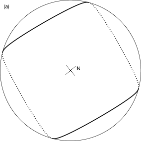
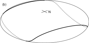
Figure 1: A simple closed geodesic for an ellipsoid with $b/a=\frac{1}{4}$. The geodesic starts on the equator with azimuth $\alpha_{0}\approx 51.24052^{\circ}$ and completes 2 complete undulations about the equator before returning to the starting longitude: (a) a top view; (b) a view at an inclination of $25^{\circ}$ to the equatorial plane; “N” marks the north pole. The solid and dotted lines show the visible and hidden portions of the geodesic.

Figure 1 illustrates a simple (i.e., non-self-intersecting) closed geodesic on an ellipsoid with $f=\frac{3}{4}$ or $b/a=\frac{1}{4}$. This is one of a class of “non-standard” closed geodesics that are neither equatorial nor meridional and which appear for sufficiently oblate ellipsoids, $a>2b$ (Klingenberg, 1982, §3.5.19).

2.3 Solving the inverse problem

The inverse problem is more challenging. Here we are given the endpoints $\phi_{1}$, $\lambda_{1}$ and $\phi_{2}$, $\lambda_{2}$, and wish to determine the shortest distance $s_{12}$ and azimuths $\alpha_{1}$ and $\alpha_{2}$. Because we have no direct way to determine $\alpha_{0}$, we must resort to an iterative solution. The traditional method for solving this problem, given by Helmert (1880) and used by Vincenty (1975), is functional iteration which fails to converge in cases where the endpoints are nearly antipodal.

A key contribution of AG was to reduce the determination of $\alpha_{0}$ to a simple one-dimensional root-finding problem. I briefly recapitulate the method here. Let’s assume we have already dealt with equatorial and meridional geodesics. Equatorial geodesics are those with $\phi_{1}=\phi_{2}=0$ and, for oblate ellipsoids, the additional condition that $\lvert\lambda_{12}\rvert\leq(1-f)\pi$; for these we have $\alpha_{1}=\pm\frac{1}{2}\pi$. Meridional geodesics are those with $\lambda_{12}=0$ or $\pm\pi$ and, for prolate ellipsoids, the additional condition that $m_{12}\geq 0$; and for these geodesics, we have $\alpha_{1}=0$ or $\pm\pi$.

For the remaining cases, we can, without loss of generality, specialize to the case

$$\phi_{1}\leq 0,\quad\phi_{1}\leq\phi_{2}\leq-\phi_{1},\quad 0<\lambda_{12}\leq\pi.$$ (16)

Note that $\lambda_{12}=0$ is excluded—this case corresponds to a meridional geodesic; the case $\lambda_{12}=\pi$ only arises for $f<0$ (for $f\geq 0$ this also corresponds to a meridional geodesic).

For a particular trial azimuth $\alpha^{*}_{1}$, we solve the hybrid problem: given $\phi_{1}$, $\alpha^{*}_{1}$, and $\phi_{2}$, compute the longitude difference $\lambda_{12}(\alpha^{*}_{1})$ corresponding to the first intersection of the geodesic with the circle of latitude $\phi_{2}$. The solution of the inverse problem is then given by finding $\alpha^{*}_{1}=\alpha_{1}$ which solves

$$\lambda_{12}(\alpha_{1})=\lambda_{12},$$ (17)

with $0<\alpha_{1}<\pi$. We use $\alpha_{1}$ as the control variable for this root-finding problem; this is a more convenient choice than $\alpha_{0}$ and, once this is found, we can readily obtain $\alpha_{0}$. In AG, we solved this equation using Newton’s method. This converges very rapidly but requires a good starting guess for the solution and this, in turn, required a careful analysis of the case of nearly antipodal endpoints.

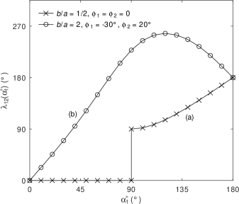
Figure 2: The solution to the hybrid problem for (a) $\phi_{1}=\phi_{2}=0$ and $b/a={\textstyle\frac{1}{2}}$ (marked with crosses); (b) $\phi_{1}=-30^{\circ}$, $\phi_{2}=20^{\circ}$, and $b/a=2$ (marked with circles). This illustrates the functional dependence of $\lambda_{12}(\alpha^{*}_{1})$.

This technique worked well with ellipsoids with small flattening. However, in the general case, the starting guess was sometimes sufficiently far from the true solution that Newton’s method failed. Before describing how we might deal with this, let us first review the properties of $\lambda_{12}(\alpha^{*}_{1})$. First of all, we have $\lambda_{12}(0)=0$ and $\lambda_{12}(\pi)=\pi$. Furthermore, with one exception, $\lambda_{12}(\alpha^{*}_{1})$ varies continuously so Eq. 17 is guaranteed to have a solution. The exception is illustrated in Fig. 2(a); this is the case with endpoints on the equator for an oblate ellipsoid and $\lambda_{12}(\alpha^{*}_{1})$ is discontinuous at $\alpha^{*}_{1}={\textstyle\frac{1}{2}}\pi$. Because equatorial and meridional geodesics have already been handled, this only occurs for ${(1-f)\pi}<\lambda_{12}<\pi$ and we can restrict the possible range of azimuth to ${\textstyle\frac{1}{2}}\pi<\alpha^{*}_{1}<\pi$. Within this range, $\lambda_{12}(\alpha^{*}_{1})$ is continuous and a solution exists. Finally, there is exactly one root and hence the derivative $\mathrm{d}\lambda_{12}(\alpha^{*}_{1})/\mathrm{d}\alpha^{*}_{1}=\lambda_{12}^{\prime}(\alpha^{*}_{1})$ is non-negative at that root. In this context, it is important to consider the case of a prolate ellipsoid; see Fig. 2(b). Even though $\lambda_{12}(\alpha^{*}_{1})$ has an interior maximum, $\lambda_{12}(\alpha^{*}_{1})=\lambda_{12}$ still has only a single root provided that $\lambda_{12}\leq\pi$ (stipulated in the initial setup of the inverse problem) and that $\alpha_{1}<\pi$ (because we have already handled meridional geodesics).

With this background, even the crudest root-finding techniques, e.g., bisection or regula falsi, can be used to find the solution. We shall continue to use Newton’s method on account of its rapid convergence. However we back it up with the bisection method to deal with two possible problems with Newton’s method: (a) $\lambda_{12}^{\prime}(\alpha^{*}_{1})$ is so small that the new value of $\alpha^{*}_{1}$ is outside the range $(0,\pi)$ or (b) $\lambda_{12}^{\prime}(\alpha^{*}_{1})$ is negative, in which case the new value of $\alpha^{*}_{1}$ is further from the true root. During the course of the Newton iteration, we maintain a bracketing range for $\alpha_{1}\in(\alpha_{1-},\alpha_{1+})$. Initially, we have $\alpha_{1-}=0$, $\alpha_{1+}=\pi$. On each iteration, we update one of $\alpha_{1\pm}$ to $\alpha^{*}_{1}$ depending on the sign of $\lambda_{12}(\alpha^{*}_{1})-\lambda_{12}$, provided that this results in a tighter bracket for $\alpha_{1}$. Whenever either of the problems, (a) or (b) listed above, occurs, we restart Newton’s method with a new starting guess $\alpha^{*}_{1}={\textstyle\frac{1}{2}}(\alpha_{1-}+\alpha_{1+})$; and we will be able to bisect the bracket after the next iteration.

We can use the spherical solution to get a starting value for $\alpha^{*}_{1}$ with a value of $0$ or $\pi$ (i.e., outside the allowed range for $\alpha_{1}$) replaced by $\frac{1}{2}\pi$. (See also Appendix A.3 for additional caveats for the case of equatorial endpoints.) Typically, the bisection safety mechanism is invoked at most once when solving the inverse problem. The net result is that this provides a reliable (always converging) and fast (rapidly converging) method of solving the inverse geodesic problem for arbitrary ellipsoids. In some cases, the inverse problem does not have a unique solution—there are multiple shortest geodesics; these cases are readily handled as discussed in Appendix A.1.

3 The area integral

3.1 Formulation of Danielsen

In AG, $S_{12}$ was defined as the area between a geodesic segment $s_{12}$ and the equator, i.e., the area of the geodesic quadrilateral $AF\!H\!B$ in Fig. 1 of AG. Following Danielsen (1989), this was cast as an integral as follows:

$$S_{12}=S(\sigma_{2})-S(\sigma_{1}),\quad S(\sigma)=c^{2}\bigl{(}\alpha+p(\sigma)\bigr{)},$$ (18)

where

$$c^{2}=\frac{a^{2}}{2}+\frac{b^{2}}{2}\frac{\tanh^{-1}e}{e}$$ (19)

is the authalic radius squared, and

$$p(\sigma) =\int_{\pi/2}^{\sigma}q(\sigma^{\prime})\,\mathrm{d}\sigma^{\prime},$$ (20)

$$q(\sigma) =-A_{4}\Delta t(e^{\prime 2},k^{2}\sin^{2}\sigma)\frac{\sin\sigma}{2},$$ (21)

$$A_{4} =\frac{e^{2}a^{2}}{c^{2}}\cos\alpha_{0}\sin\alpha_{0},$$ (22)

$$\Delta t(x,y) =\frac{t(x)-t(y)}{x-y},$$ (23)

$$t(x) =x+\sqrt{1+x}\,\frac{\sinh^{-1}\sqrt{x}}{\sqrt{x}}.$$ (24)

This is a change from the notation in Eq. (59) of AG; the relationship is

$$p(\sigma)=A_{4}I_{4}(\sigma);$$ (25)

this simplifies the assessment of the error in $S_{12}$. The expression $\Delta t(x,y)$ is the divided difference of $t(x)$. In the limit $y\rightarrow x$, we have $\Delta t(x,x)=t^{\prime}(x)$. If $x$ and $y$ are distinct and have the same sign, there’s a systematic way to express $\Delta t(x,y)$ in a form that avoids excessive roundoff errors (Kahan and Fateman, 1999).

The area of an arbitrary geodesic polygon is easily computed by summing the signed area contributions $S_{12}$ for each edge. An adjustment to this total needs to be made if the polygon encircles a pole as described in AG.

The challenge is that the integral, Eq. (20), cannot be carried out in closed form. However both $q(\sigma)$ and $p(\sigma)$ are periodic functions and so may be written as Fourier series:

$$q(\sigma) =\sum_{l=0}^{\infty}Q_{l}\sin\bigl{(}2(l+{\textstyle\frac{1}{2}})\sigma\bigr{)},$$ (26)

$$Q_{l} =\frac{4}{\pi}\int_{0}^{\pi/2}q(\sigma)\sin\bigl{(}2(l+{\textstyle\frac{1}{2}})\sigma\bigr{)}\,\mathrm{d}\sigma,$$ (27)

$$p(\sigma) =\sum_{l=0}^{\infty}P_{l}\cos\bigl{(}2(l+{\textstyle\frac{1}{2}})\sigma\bigr{)},$$ (28)

$$P_{l} =-\frac{Q_{l}}{2(l+\frac{1}{2})}.$$ (29)

Here, Eqs. (26) and (27) constitute a Fourier transform pair. In the next sections, we explore two ways to compute $P_{l}$ approximately.

3.2 Using a Taylor series

In AG, we gave Taylor series expansions for $P_{l}$ using $e^{\prime 2}$ and $k^{2}$ as small parameters. For reasons explained in Appendix A.5, this is a poor choice of expansion parameters for eccentric ellipsoids; so we replace the expansion parameters by $n$ and $\epsilon$, Eqs. (43), resulting in the expansion Eqs. (44) which should be used instead of AG’s Eqs. (63). This expansion may be used to approximate $p(\sigma)$ with

$$\tilde{p}^{(N)}(\sigma) =\sum_{l=0}^{\infty}\tilde{P}_{l}^{(N)}\cos\bigl{(}2(l+{\textstyle\frac{1}{2}})\sigma\bigr{)},$$ (30)

$$\tilde{P}_{l}^{(N)} =A_{4}C_{4l},$$ (31)

where $A_{4}$ is defined in Eq. (22) and the superscript $(N)$ gives the order at which the Taylor series is truncated; thus Eqs. (44) with the ellipses dropped corresponds to $N=6$. $A_{4}$ is proportional to $e^{2}$, so the highest order terms in Eqs. (44) are $O(f^{6})$; furthermore, we have $\tilde{P}_{l}^{(N)}=0$ for $l\geq N$.

One possibility for computing the area on eccentric ellipsoids is extending the Taylor series expansion to higher order. Thus, when I first implemented the solution of the geodesic problem in terms of elliptic integrals as described in Sec. 2, I computed the area using $\tilde{p}^{(30)}(\sigma)$; this gives full double precision accuracy for ${\textstyle\frac{1}{2}}\leq b/a\leq 2$. However, this approach quickly becomes cumbersome for extremely eccentric ellipsoids:

• the value of $N$ required to give full accuracy becomes very large;

• the cost of determining the coefficients in the Taylor series becomes impractical—it takes Maxima (2022) 17 minutes for $N=32$ (tolerable for generating code) but 19 hours to extend this to $N=64$ (which is starting to get painful);

• the storage required for the coefficients becomes excessive, scaling as $N^{3}/6$;

• once the ellipsoid is selected, evaluating the coefficients of $\epsilon^{j}$ in Eqs. (44) requires $O(N^{3})$ operations;

• once $\alpha_{0}$ is given, evaluating $\tilde{P}_{l}^{(N)}$ requires $O(N^{2})$ operations.

3.3 Quadrature using discrete sine transforms

To overcome the shortcomings of Taylor series for large eccentricities, I explored evaluating Eq. (20) using the quadrature method of Clenshaw and Curtis (1960). Given a definite integral,

$$\int_{-1}^{1}g(x)\,\mathrm{d}x,$$

this method entails expanding $g(x)$ as Chebyshev polynomials, or, equivalently, $g(\cos\theta)$ as a Fourier series. This allows the definite integral to be computed to high accuracy and, as a bonus, the indefinite integral can be computed. The accuracy is a result of the fast convergence of the trapezoidal rule for integrals of a periodic function over a full period; in this case, the integrals give the Fourier coefficients.

However, this is a roundabout procedure given that we are starting with a periodic function. Instead, we directly evaluate Eq. (27) using the trapezoidal rule and evaluate $p(\sigma)$ by using the resulting Fourier coefficients in Eqs. (28) and (29). Thus we approximate $Q_{l}$ with

$$\hat{Q}_{l}^{(N)}=\frac{4h_{N}}{\pi}\operatorname*{\sum\nolimits^{\prime}}_{j=0}^{N-1}q((j+1)h_{N})\sin\bigl{(}2(l+{\textstyle\frac{1}{2}})(j+1)h_{N}\bigr{)},$$ (32)

where $h_{N}=\pi/(2N)$, we take $0\leq l<N$, and the prime on the summation sign indicates that the last term in the sum should be halved. Because $q(\sigma)$ is an analytic periodic function, $\hat{Q}_{l}^{(N)}$ converges to the true value $Q_{l}$ faster than any power of $N$, as $N\rightarrow\infty$. Equation (32) is, in fact, the discrete sine transform, DST, of type III (Wang and Hunt, 1985). Its inverse is a type II DST,

$$q((j+1)h_{N})=\sum_{l=0}^{N-1}\hat{Q}_{l}^{(N)}\sin\bigl{(}2(l+{\textstyle\frac{1}{2}})(j+1)h_{N}\bigr{)};$$ (33)

this holds for all integer $j$. Rewriting this as a continuous function,

$$\hat{q}^{(N)}(\sigma)=\sum_{l=0}^{N-1}\hat{Q}_{l}^{(N)}\sin\bigl{(}2(l+{\textstyle\frac{1}{2}})\sigma\bigr{)},$$ (34)

we see that $\hat{q}^{(N)}(\sigma)$ is likely to be an excellent approximation to $q(\sigma)$ given that the functions coincide wherever $\sigma$ is a multiple of $h_{N}$. In the same way, we approximate $p(\sigma)$ by

$$\hat{p}^{(N)}(\sigma) =\sum_{l=0}^{\infty}\hat{P}_{l}^{(N)}\cos\bigl{(}2(l+{\textstyle\frac{1}{2}})\sigma\bigr{)},$$ (35)

$$\hat{P}_{l}^{(N)} =\begin{cases}\displaystyle-\frac{\hat{Q}_{l}^{(N)}}{2(l+\frac{1}{2})},&\text{for $l<N$},\\ 0,&\text{for $l\geq N$}.\end{cases}$$ (36)

A convenient way to compute DSTs is using the fast Fourier transform, FFT (Cooley and Tukey, 1965). This reduces the cost of evaluating Eq. (32) for $0\leq l<N$ from $O(N^{2})$ to $O(N\log N)$. Furthermore, Gentleman (1972) points out that the FFT results in smaller roundoff errors compared with other methods. Equation (35) can be evaluated using Clenshaw (1955) summation; this method is fast (the cosine terms are computed by a recurrence relation) and because $\hat{Q}_{l}^{(N)}$ decays rapidly with $l$ and because the summation starts at high values of $l$, it is also accurate.

As we shall see, the error $\max(\lvert\hat{q}^{(N)}(\sigma)-q(\sigma)\rvert)$ decays exponentially with $N$; thus doubling $N$ roughly squares the error. Furthermore, it’s possible to double $N$ rather inexpensively. First, generate the type IV DST for $q(\sigma)$,

$$\check{Q}_{l}^{(N)}=\frac{4h_{N}}{\pi}\sum_{j=0}^{N-1}q((j+{\textstyle\frac{1}{2}})h_{N})\sin\bigl{(}2(l+{\textstyle\frac{1}{2}})(j+{\textstyle\frac{1}{2}})h_{N}\bigr{)}.$$ (37)

The sums for computing $\hat{Q}_{l}^{(N)}$, Eq. (32), and $\check{Q}_{l}^{(N)}$ involve evaluating $q(\sigma)$ at intervals of ${\textstyle\frac{1}{2}}h_{N}=h_{2N}$; it follows that $\hat{Q}_{l}^{(2N)}$ is just the mean of $\hat{Q}_{l}^{(N)}$ and $\check{Q}_{l}^{(N)}$. These coefficients for $N\leq l<2N$ are

$$\hat{Q}_{l}^{(N)}=-\hat{Q}_{2N-1-l}^{(N)},\quad\check{Q}_{l}^{(N)}=+\check{Q}_{2N-1-l}^{(N)}.$$ (38)

Thus, $\hat{Q}_{l}^{(2N)}$ is given by

$$\hat{Q}_{N-1/2\pm g}^{(2N)}=\frac{\check{Q}_{N-1/2-\lvert g\rvert}^{(N)}\mp\hat{Q}_{N-1/2-\lvert g\rvert}^{(N)}}{2},$$ (39)

for $g=\frac{1}{2},\frac{3}{2},\ldots,N-\frac{1}{2}$. This method avoids wasting the results $\hat{Q}_{l}^{(N)}$ which have already been computed (Gentleman, 1972).

3.4 Convergence of approximate Fourier series

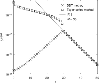
Figure 3: The dependence of the errors in the individual Fourier coefficients, $P_{l}$, on $l$ for $N=30$. The crosses, resp. squares, show the errors using the DST method, $\delta\hat{P}_{l}^{(N)}$, resp. the Taylor series method, $\delta\tilde{P}_{l}^{(N)}$. The case illustrated is for a geodesic on an ellipsoid with $b/a=\frac{1}{4}$, $\alpha_{0}=\frac{1}{4}\pi$. The line shows the exact value of $\lvert P_{l}\rvert$.

In assessing how well $\hat{p}^{(N)}(\sigma)$, Eq. (35), approximates $p(\sigma)$, we start by looking at the error in the individual Fourier coefficients, namely $\delta\hat{P}_{l}^{(N)}=\lvert\hat{P}_{l}^{(N)}-P_{l}\rvert$ for a given $N$. For illustrative purposes, we consider $b/a=\frac{1}{4}$, $\alpha_{0}=\frac{1}{4}\pi$, and consider $N=30$; we compute the “exact” $P_{l}$ using a much larger value $N$. The resulting errors $\delta\hat{P}_{l}^{(30)}$ are shown in Fig. 3 as crosses. The figure also shows $\lvert P_{l}\rvert$ (the solid line) decaying exponentially as a function of $l$. Obviously $\delta\hat{P}_{l}^{(30)}$, which equals $\lvert P_{l}\rvert$ for $l\geq 30$, shows the same exponential decay. However, we also have exponential decay in $\delta\hat{P}_{l}^{(30)}$ as $l$ decreases from $29$ to $0$; indeed, $\delta\hat{P}_{l}^{(30)}$ is roughly symmetric about $l=30$. This behavior is predicted by Eq. (39), since we can approximate $\delta\hat{P}_{l}^{(N)}$ by $\lvert\hat{P}_{l}^{(N)}-\hat{P}_{l}^{(2N)}\rvert$, with

$$\hat{P}_{N-1/2\pm g}^{(N)}-\hat{P}_{N-1/2\pm g}^{(2N)}=\frac{\hat{Q}_{N-1/2-\lvert g\rvert}^{(N)}-\check{Q}_{N-1/2-\lvert g\rvert}^{(N)}}{4(N\pm g)};$$ (40)

the variation of the numerator in this expression (symmetric in $g$) is much stronger than the variation of the denominator. We conclude that the error arising from using approximate Fourier coefficients, $\hat{P}_{l}^{(N)}$ instead of $P_{l}$, is approximately the same as the error from truncating the Fourier sum in Eq. (35).

Figure 3 also shows the errors in the Taylor series coefficients $\delta\check{P}_{l}^{(N)}=\lvert\check{P}_{l}^{(N)}-P_{l}\rvert$ for $N=30$ as squares. The error is, of course, the same as for $\delta\hat{P}_{l}^{(30)}$ for $l\geq 30$; but for $l<30$, the error is several orders of magnitude bigger.

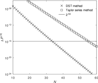
Figure 4: The dependence of the overall error in the Fourier series approximation to $p(\sigma)$ on $N$. The crosses, resp. squares, show the errors for the DST method, $\Delta\hat{P}^{(N)}$, resp. the Taylor series method, $\Delta\tilde{P}^{(N)}$. This is for the same case as Fig. 3, namely $b/a=\frac{1}{4}$, $\alpha_{0}=\frac{1}{4}\pi$. The horizontal line indicates the roundoff limit for double precision $2^{-53}\approx 10^{-16}$.

Figure 3 gives the errors in the individual Fourier coefficients for a particular $N$. To gauge how the overall error in $\hat{p}^{(N)}(\sigma)$, Eq. (35), varies with $N$, we combine the errors in the coefficients, as follows,

$$\Delta\hat{P}^{(N)}=\sum_{l=0}^{\infty}\delta\hat{P}_{l}^{(N)}.$$ (41)

We similarly define $\Delta\tilde{P}^{(N)}$ for the coefficients obtained by Taylor expansion. Figure 4 shows how these error metrics vary as $N$ is increased from $10$ to $60$ for $b/a=\frac{1}{4}$ and $\alpha_{0}=\frac{1}{4}\pi$ (the same parameters used for Fig. 3). Both show exponential decay with $\Delta\hat{P}^{(N)}$ being several orders of magnitude smaller and decaying at a slightly faster rate.

3.5 Determining the number of points in the quadrature

In practical applications, we will evaluate the area using Eqs. (18) and have to contend both with truncation errors, because we use a finite value of $N$ in computing $p(\sigma)$, and with roundoff errors, because of the limited precision of the floating-point number system. We would like to pick $N$ large enough that the truncation errors are less than the roundoff errors and for this we require that $\Delta\hat{P}^{(N)}\leq 2^{-m}$ where $m$ is the number of bits in the fraction of a floating-point number. For double precision, we typically have $m=53$ and, substituting the value of $c\approx 6371\,\mathrm{km}^{2}$ for the earth, this gives a truncation error in $S(\sigma)$ of $2^{-53}c^{2}\approx 50\,\mathrm{cm}^{2}$. The horizontal line in Fig. 4 labels this error threshold, $2^{-53}$. This shows that, for this case, we need $N\geq 34$ for the DST method compared to $N\geq 56$ when using a Taylor expansion.

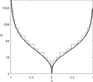
Figure 5: The heavy line shows the minimum number of points $N$ required in the DST to ensure double precision accuracy as a function of $n$ for $\lvert n\rvert\leq 0.99$ and for arbitrary $\alpha_{0}$. If we limit the possible values of $N$ to $2\times 2^{j}$ and $3\times 2^{j}$ with integer $j\geq 1$, then the result is the staircase shown as a light line.

In principle, we could reestimate $N$ for each geodesic, i.e., for every $n$ and $\alpha_{0}$. (Since we are dealing with both oblate and prolate ellipsoids of arbitrary eccentricity, we use $n$ as the measure of eccentricity instead of $e=2\sqrt{n}/(1+n)$ or $f=2n/(1+n)$.) However, that would require extra machinery to do the estimation at run time. Instead, we estimate $N$ for $-0.99\leq n\leq 0.99$. For a particular $n$, we find the minimum $N$ that satisfies the accuracy requirement for all $\alpha_{0}$. The result is shown in Fig. 5 as the heavy line. The light line shows the result of restricting the allowed values of $N$ to $2\times 2^{j}$ and $3\times 2^{j}$ with integer $j\geq 1$; now $N$ is the product of small factors ($2$ and $3$), a requirement for the efficient implementation of the FFT. The light line is converted to a simple table allowing $N$ to be looked up at run time based on the value of $n$.

The conclusion is that the discrete sine transform method provides a convenient and accurate way to evaluate the area integral. In comparison to the Taylor series method: the same accuracy is obtained with substantially fewer terms ($N=34$ for the DST versus $N=56$ for the Taylor series in the example illustrated in Fig. 4). Just as important, $N$ can be easily adjusted for a particular $n$, Fig. 5 (no need to compute a new Taylor series), the memory required is $O(N)$ instead of $O(N^{3})$, and the setup time for a particular geodesic is $O(N\log N)$ instead of $O(N^{3})$.

4 Implementation

The algorithms detailed in Secs. 2 and 3 have been implemented in version 2.1.2 of the open-source C++ library, GeographicLib (Karney, 2022). The solution of the geodesic problems in terms of elliptic integrals was added in version 1.25 (2012). At that time, the area was computed with a 30th order Taylor series as described in Sec. 3.2. This was replaced by the implementation using DSTs, Sec. 3.3, in version 2.1 (2022). These algorithms supplemented the earlier ones described in AG since, as we see below, these remain the preferred methods for terrestrial ellipsoids.

We use the KISS FFT package (Boergerding, 2021) for performing the DST. Even though this package has no direct support for the DSTs, as a “header-only” package, it is easier to integrate into GeographicLib than the more capable FFTW package (Frigo and Johnson, 2021).

The main geodesic calculations are also exposed with two utility programs provided with GeographicLib, GeodSolve for geodesic calculations, and Planimeter for measuring the perimeter and area of geodesic polygons. With both utilities, the -E flag uses the algorithms described here for arbitrary ellipsoids.

In developing numerical algorithms, especially those that offer high accuracy, it is very useful to be able to distinguish truncation errors from roundoff errors. For this reason, high precision calculations were added to GeographicLib in version 1.37 (2014). This allowed the library to be compiled with various alternatives to standard double precision (53 bits of precision or 16 decimal digits) for floating-point numbers:

• extended precision (64 bits or 19 decimal digits) available as the “long double” type on some platforms;

• quadruple precision (113 bits or 34 decimal digits) using the boost multi-precision library (Maddock and Kormanyos, 2022);

• arbitrary precision (selected at the start of execution) using the MPREAL C++ interface (Holoborodko, 2022) to the MPFR library (Fousse et al., 2007).

The results in Figs. 3, 4, and 5 and in Tables 1 and 2, below, were computed with the last option setting the precision to 256 bits (77 decimal digits).

5 Results

A starting point for testing the new algorithms is the test data set given in Karney (2010). This is specific to the WGS84 ellipsoid and as such allows us to compare the new algorithms with the series solutions described in AG. The maximum errors in geodesic calculations when converted to a distance are about $0.03\,\mu\mathrm{m}$ which is 2–3 times larger than the corresponding figures for the series solution. The error in the area is about $0.1\,\mathrm{m}^{2}$ in both cases. On this data set the new routines run about 2.5 times slower. The lower accuracy and speed are to be expected given the additional complexity of the new algorithms.

The lesson is clear: for terrestrial ellipsoids, the algorithms described in AG are to be preferred—they are faster and more accurate than the new routines. In fact, the new routines are still very accurate and fast. Once the eccentricity of the ellipsoid is such that $\lvert f\rvert>\frac{1}{50}$, the accuracy of the series solution degrades and the new routines should be used. Let us, therefore, turn to assessing their performance on eccentric ellipsoids.

Table 1: Results for a geodesic segment with $\phi_{1}=0$, $\lambda_{1}=0$, $\alpha_{1}=\frac{1}{4}\pi$, $\sigma_{12}={\textstyle\frac{1}{2}}\pi$ on an oblate ellipsoid with $a=6\,400\,\mathrm{km}$ and with various values of the third flattening, $n$. For each value of $n$, the first, resp. second, row gives the results of a high precision, resp. double precision, calculation. The data is displayed with 17 decimal digits and all the digits in the first rows may be regarded as correct. The differing digits in the second row are underlined, but differences in the 17th digit are usually not significant. The analytic results for $n=0$ and $1$ are also given.

$n$	$\lambda_{2}\,({}^{\circ})$	$s_{12}\,(\mathrm{m})$	$S_{12}\,(\mathrm{m}^{2})$
$0$	$90$	${\textstyle\frac{1}{2}}\pi a$	$\frac{1}{4}\pi a^{2}$
$\scriptstyle 0.01$	$\scriptstyle 88.742968019148302$	$\scriptstyle 9904105.0587012822$	$\scriptstyle 31213542356109.085$
	$\scriptstyle 88.74296801914830\underline{7}$	$\scriptstyle 9904105.05870128\underline{80}$	$\scriptstyle 31213542356109.0\underline{90}$
$\scriptstyle 0.02$	$\scriptstyle 87.516869281406891$	$\scriptstyle 9758656.5485393260$	$\scriptstyle 30293469475840.470$
	$\scriptstyle 87.5168692814068\underline{83}$	$\scriptstyle 9758656.54853932\underline{56}$	$\scriptstyle 30293469475840.4\underline{69}$
$\scriptstyle 0.05$	$\scriptstyle 84.015774978368889$	$\scriptstyle 9342609.4418442232$	$\scriptstyle 27735488324240.197$
	$\scriptstyle 84.0157749783688\underline{96}$	$\scriptstyle 9342609.44184422\underline{12}$	$\scriptstyle 27735488324240.19\underline{5}$
$\scriptstyle 0.10$	$\scriptstyle 78.725380139212172$	$\scriptstyle 8711622.0524734494$	$\scriptstyle 24064301808040.490$
	$\scriptstyle 78.7253801392121\underline{63}$	$\scriptstyle 8711622.05247344\underline{26}$	$\scriptstyle 24064301808040.4\underline{88}$
$\scriptstyle 0.20$	$\scriptstyle 69.896175299112817$	$\scriptstyle 7650604.1274847332$	$\scriptstyle 18453877989937.629$
	$\scriptstyle 69.8961752991128\underline{26}$	$\scriptstyle 7650604.1274847332$	$\scriptstyle 18453877989937.62\underline{5}$
$\scriptstyle 0.40$	$\scriptstyle 57.573823093058582$	$\scriptstyle 6143630.9790943809$	$\scriptstyle 11678681837788.421$
	$\scriptstyle 57.57382309305858\underline{6}$	$\scriptstyle 6143630.9790943\underline{796}$	$\scriptstyle 11678681837788.42\underline{2}$
$\scriptstyle 0.60$	$\scriptstyle 50.239779898617183$	$\scriptstyle 5219414.0281749099$	$\scriptstyle 8187126653111.4930$
	$\scriptstyle 50.239779898617\underline{222}$	$\scriptstyle 5219414.0281749\underline{116}$	$\scriptstyle 8187126653111.49\underline{80}$
$\scriptstyle 0.90$	$\scriptstyle 45.355849749995502$	$\scriptstyle 4575456.8211684255$	$\scriptstyle 6010343299883.0257$
	$\scriptstyle 45.355849749995\underline{450}$	$\scriptstyle 4575456.8211684255$	$\scriptstyle 6010343299883.025\underline{4}$
$\scriptstyle 0.95$	$\scriptstyle 45.098003329505353$	$\scriptstyle 4539479.1711295677$	$\scriptstyle 5891663480815.9028$
	$\scriptstyle 45.098003329505\underline{410}$	$\scriptstyle 4539479.171129567\underline{5}$	$\scriptstyle 5891663480815.90\underline{62}$
$\scriptstyle 0.98$	$\scriptstyle 45.017931867960028$	$\scriptstyle 4528085.2709957805$	$\scriptstyle 5853723375274.4502$
	$\scriptstyle 45.0179318679\underline{59945}$	$\scriptstyle 4528085.270995780\underline{8}$	$\scriptstyle 5853723375274.45\underline{31}$
$\scriptstyle 0.99$	$\scriptstyle 45.004943101537128$	$\scriptstyle 4526207.1227753328$	$\scriptstyle 5847407841550.2810$
	$\scriptstyle 45.004943101537\underline{080}$	$\scriptstyle 4526207.122775332\underline{1}$	$\scriptstyle 5847407841550.28\underline{52}$
$1$	$45$	$a/\sqrt{2}$	$\frac{1}{8}(\pi-2)a^{2}$

Table 2: Analogous results to Table 1, but for prolate ellipsoids. Here the values for $S_{12}$ for $-n\geq 0.98$ exceed $10^{17}\,\mathrm{m}^{2}$ and these are displayed to the nearest whole square meter, i.e., 18 decimal digits.

$-n$	$\lambda_{2}\,({}^{\circ})$	$s_{12}\,(\mathrm{m})$	$S_{12}\,(\mathrm{m}^{2})$
$\scriptstyle 0.01$	$\scriptstyle 91.288854749527201$	$\scriptstyle 10205732.514416281$	$\scriptstyle 33164247992795.212$
	$\scriptstyle 91.288854749527\underline{189}$	$\scriptstyle 10205732.514416281$	$\scriptstyle 33164247992795.21\underline{1}$
$\scriptstyle 0.02$	$\scriptstyle 92.610457370098315$	$\scriptstyle 10362118.908653340$	$\scriptstyle 34198331462649.689$
	$\scriptstyle 92.61045737009831\underline{7}$	$\scriptstyle 10362118.9086533\underline{39}$	$\scriptstyle 34198331462649.6\underline{95}$
$\scriptstyle 0.05$	$\scriptstyle 96.781576904333249$	$\scriptstyle 10854904.416431548$	$\scriptstyle 37558272805333.618$
	$\scriptstyle 96.7815769043332\underline{35}$	$\scriptstyle 10854904.4164315\underline{50}$	$\scriptstyle 37558272805333.6\underline{25}$
$\scriptstyle 0.10$	$\scriptstyle 104.48653831623701$	$\scriptstyle 11762457.095994598$	$\scriptstyle 44149951026541.638$
	$\scriptstyle 104.4865383162370\underline{0}$	$\scriptstyle 11762457.095994\underline{601}$	$\scriptstyle 44149951026541.6\underline{48}$
$\scriptstyle 0.20$	$\scriptstyle 123.32603446808286$	$\scriptstyle 13970425.888241007$	$\scriptstyle 62377755412860.708$
	$\scriptstyle 123.3260344680828\underline{5}$	$\scriptstyle 13970425.88824100\underline{2}$	$\scriptstyle 62377755412860.70\underline{3}$
$\scriptstyle 0.40$	$\scriptstyle 182.39739178709022$	$\scriptstyle 20839831.771249872$	$\scriptstyle 139011560027117.22$
	$\scriptstyle 182.3973917870902\underline{1}$	$\scriptstyle 20839831.7712498\underline{68}$	$\scriptstyle 139011560027117.2\underline{8}$
$\scriptstyle 0.60$	$\scriptstyle 304.70849870674712$	$\scriptstyle 34975034.400175888$	$\scriptstyle 391742895540755.96$
	$\scriptstyle 304.7084987067471\underline{5}$	$\scriptstyle 34975034.4001758\underline{69}$	$\scriptstyle 391742895540755.9\underline{4}$
$\scriptstyle 0.90$	$\scriptstyle 1428.1147116097373$	$\scriptstyle 164323044.22719251$	$\scriptstyle 8648966122417968.8$
	$\scriptstyle 1428.114711609737\underline{9}$	$\scriptstyle 164323044.2271925\underline{2}$	$\scriptstyle 86489661224179\underline{73.0}$
$\scriptstyle 0.95$	$\scriptstyle 2929.9802152369325$	$\scriptstyle 337162015.21658508$	$\scriptstyle 36412212193071484$
	$\scriptstyle 2929.9802152369\underline{275}$	$\scriptstyle 337162015.21658\underline{468}$	$\scriptstyle 364122121930714\underline{24}$
$\scriptstyle 0.98$	$\scriptstyle 7436.6985105821765$	$\scriptstyle 855784235.25896030$	$\scriptstyle 234584335066399637$
	$\scriptstyle 7436.6985105821\underline{568}$	$\scriptstyle 855784235.2589\underline{5941}$	$\scriptstyle 234584335066399\underline{136}$
$\scriptstyle 0.99$	$\scriptstyle 14948.252975667299$	$\scriptstyle 1720188142.2370088$	$\scriptstyle 947812505054464151$
	$\scriptstyle 14948.2529756672\underline{32}$	$\scriptstyle 1720188142.23700\underline{64}$	$\scriptstyle 94781250505446\underline{5024}$

We start by considering the geodesic that starts on the equator, i.e., at its node $\phi_{1}=0$, with azimuth $\alpha_{0}=\alpha_{1}=\frac{1}{4}\pi$ and compute the longitude at the vertex (the point of maximum latitude), the distance to the vertex, and the area under this geodesic segment. We shall carry out this calculation with various values of the third flattening $n$. The arc length on the auxiliary sphere, in this case, is $\sigma_{12}={\textstyle\frac{1}{2}}\pi$, and, because $\tan\alpha_{0}=1$, we have $\tan\phi_{2}=(1+n)/(1-n)$.

The results are shown in Tables 1 and 2 for oblate and prolate ellipsoids respectively. For each $n$, the first row shows the results with high precision arithmetic rounded to 17 decimal digits. These allow independent verification of the algorithms. The second row shows the results of carrying out the calculation in double precision. In all cases, the roundoff errors are very small—the changes take place in no more than the last 5 bits of the fraction of the binary representation; with $\lvert n\rvert\leq 0.9$, the errors amount to at most 7 units in the last place in the binary representation.

A more challenging test is presented with the data for the administrative boundaries of Poland (this was kindly provided to me in 2013 by Paweł Pędzich of the Warsaw University of Technology). This set includes a polygonal representation of the boundary of Poland itself. This consists of $67\,801$ edges with mean length $53\,\mathrm{m}$, minimum length $62\,\mathrm{mm}$, and maximum length $9.7\,\mathrm{km}$; the perimeter of the polygon is about $3\,600\,\mathrm{km}$ and its area is about $313\,000\,\mathrm{km}^{2}$. This is a good test for geodesic algorithms as it represents a realistic “large” problem allowing the overall accuracy and speed of the algorithms to be assessed.

In performing tests on ellipsoids with varying eccentricities, we need to stipulate how the points are mapped onto the ellipsoid. If we merely keep the latitude fixed, then for extreme oblate, resp. prolate, ellipsoids, all the points end up concentrated near the equator, resp. the poles, making it difficult to interpret the results. We instead map the points keeping the authalic latitude fixed. If, in addition, we choose $a$ so that the area of the ellipsoid matches that of the Earth, the area of the polygon is nearly constant as $n$ is varied and we assess the errors by computing the difference between the computed area and the true area. For this exercise, we find the true area using quadruple precision arithmetic.

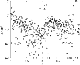
Figure 6: The absolute errors in the calculation of the area $\Delta A$ (plus signs, scale on the left) and perimeter $\Delta P$ (diamonds, scale on the right) of a polygonal model of Poland. Here the model is mapped to ellipsoids with various eccentricities (denoted by the third flattening $n$) by preserving the value of the authalic latitude.

The errors in the area and the perimeter are shown in Fig. 6. Generally speaking the errors in the area are between $1\,\mathrm{m}^{2}$ and $10\,\mathrm{m}^{2}$ and the errors in the perimeter are between $1\,\mu\mathrm{m}$ and $3\,\mu\mathrm{m}$.

The elapsed time for these calculations is approximated by

$$\bigl{(}4.5+N(40+\log_{2}N)/450\bigr{)}\,\mathrm{\mu s}\text{ per edge},$$

where the first term represents the time to compute the perimeter of the polygon, which involves solving the inverse geodesic problem for an edge, and the second term is the additional time required to compute its area. Here $N$ is the number of terms used in the DST which is given in Fig. 5. The time to compute the area begins to dominate for $\lvert n\rvert>0.2$. The area calculation could be made faster if the DSTs were computed using the FFTW package instead of KISS FFT.

6 Discussion

In this paper, we have shown how to solve geodesic problems on an ellipsoid of arbitrary eccentricity and an implementation of these methods is available in GeographicLib. The work naturally divides into two parts:

The method of solving the standard direct and inverse problems was an exercise in applying Carlson’s algorithms for the evaluation of elliptic integrals to the work of Legendre and Cayley. These then replaced the Taylor series expansions for the elliptic integrals used in AG. In addition, the method for solving the inverse problem needed to be adjusted to ensure convergence in all cases.

The evaluation of the area integral, Eq.(20), is simplicity itself: write the periodic integrand as a Fourier series, evaluate the Fourier coefficients by trapezoidal quadrature, and then the integral of the resulting series is trivial. This is an accurate and fast method because (1) the Fourier series of an analytic function converges rapidly, (2) quadrature is very accurate when applied to the full period of a periodic function, (3) the FFT can be used to evaluate all the coefficients efficiently. This method will be useful in other applications, e.g., to evaluate the Abelian integrals appearing in the solution given by Jacobi (1839) for geodesics on a triaxial ellipsoid.

The algorithms have been tested for a wide range of eccentricities, $\lvert n\rvert\leq 0.99$ or $1/199\leq b/a\leq 199$; this encompasses ellipsoids flatter than a pancake and as thin as spaghetti. In principle, the methods would work at more extreme eccentricities; however, it is likely a more specialized approach would be better in these cases. Despite this, the Taylor series method described in AG is preferred for small flattening, $\lvert f\rvert\leq\frac{1}{50}$. This is somewhat more accurate and somewhat faster than the general method given here.

The obvious domain of application for these algorithms is studying planets and other celestial bodies with high eccentricity. But, they also play a role in terrestrial applications. First of all, they allow the errors in the Taylor series method to be measured accurately. Secondly, because the flattening of terrestrial ellipsoids is so small, a starting approximation to the solution is given by spherical trigonometry and this solution can be subsequently refined using ellipsoidal geodesics. Unfortunately, any specifically ellipsoidal behavior might be overlooked, precisely because the flattening is small. Therefore, it behooves the developer to test the algorithms on more eccentric ellipsoids, say, with $f=\frac{1}{5}$, because then any ellipsoid effects will be much more apparent.

Appendix A Addenda to Karney (2013)

A.1 Multiple shortest geodesics

The shortest distance found by solving the inverse problem is (obviously) uniquely defined. However, in some special cases, multiple azimuths yield the same shortest distance. Here is a catalog of those cases:

• $\phi_{1}=-\phi_{2}$ (with neither point at a pole): If $\alpha_{1}=\alpha_{2}$, the geodesic is unique. Otherwise, there are two geodesics and the second one is obtained by setting $[\alpha_{1},\alpha_{2}]\leftarrow[\alpha_{2},\alpha_{1}]$, $[M_{12},M_{21}]\leftarrow[M_{21},M_{12}]$, and $S_{12}\leftarrow-S_{12}$. (This occurs when $\lambda_{12}$ is close to $\pm 180^{\circ}$ for oblate ellipsoids.)

• $\lambda_{12}=\pm 180^{\circ}$ (with neither point at a pole). If $\alpha_{1}=0^{\circ}$ or $\pm 180^{\circ}$, the geodesic is unique. Otherwise, there are two geodesics and the second one is obtained by setting $[\alpha_{1},\alpha_{2}]\leftarrow[-\alpha_{1},-\alpha_{2}]$, $S_{12}\leftarrow-S_{12}$. (This occurs when $\phi_{2}$ is close to $-\phi_{1}$ for prolate ellipsoids.)

• points 1 and 2 are at opposite poles: There are infinitely many geodesics that can be generated by setting $[\alpha_{1},\alpha_{2}]\leftarrow[\alpha_{1},\alpha_{2}]+[\delta,-\delta]$, for arbitrary $\delta$. (For spheres, this prescription applies when points 1 and 2 are antipodal.)

• $s_{12}=0$ (coincident points): There are infinitely many geodesics that can be generated by setting $[\alpha_{1},\alpha_{2}]\leftarrow[\alpha_{1},\alpha_{2}]+[\delta,\delta]$, for arbitrary $\delta$.

In cases where there are multiple shortest geodesics, GeographicLib returns an arbitrary one. The list given above allows the user (a) to determine whether there are other shortest geodesics and (b) to generate them.

A.2 Refining the result from the reverted distance series

The 6th-order series given in AG provide solutions for the geodesic problem which are accurate to roundoff for $\lvert f\rvert\leq\frac{1}{100}$. The least accurate of the series is the reverted series for $\sigma$ in terms of the scaled distance $\tau$, Eqs. (20) and (21) of AG, which is used only in solving the direct problem. (This series also gives the reduced latitude $\beta$ in terms of the rectifying latitude $\mu$.) The accuracy is improved by using these equations to give an initial approximation for $\sigma$ which is followed by one step of Newton’s method applied to Eq. (4), with $\mathrm{d}s/\mathrm{d}\sigma=b\sqrt{1+k^{2}\sin^{2}\sigma}$. With this change (which need only be applied for $\lvert f\rvert>\frac{1}{100}$), the 6th-order series are accurate to roundoff for $\lvert f\rvert\leq\frac{1}{50}$.

A.3 Non-equatorial geodesics

Care needs to be taken when solving the inverse problem for a non-equatorial geodesic when both endpoints are on the equator. If $\phi_{1}=\phi_{2}=0$, set $\phi_{1}=-0$ when determining $\sigma_{1}$ and $\omega_{1}$ using Eqs. (11) and (12) of AG. The library function atan2 will use the sign of zero to determine the correct quadrant. In addition, $\alpha_{1}={\textstyle\frac{1}{2}}\pi$ should be treated as $\alpha_{1}={\textstyle\frac{1}{2}}\pi+\delta$ (e.g., by setting $\cos\alpha_{1}$ to some tiny negative value $-\delta$); this breaks the degeneracy in the equation for $\sigma_{1}$.

A.4 An improved series for $A_{2}$

The series for $A_{2}$, Eq. (42) in AG, converges slightly faster if we expand ${(1+\epsilon)}A_{2}$, instead of $A_{2}/{(1-\epsilon)}$. The resulting series is

$$\textstyle A_{2}=(1+\epsilon)^{-1}\bigl{(}1-\frac{3}{4}\epsilon^{2}-\frac{7}{64}\epsilon^{4}-\frac{11}{256}\epsilon^{6}+\ldots\bigr{)}.$$ (42)

A.5 Re-expansion of the area integral

Equations (63) of AG give coefficients $C_{4l}$ for the Fourier series for the area integral. These are Taylor series with $e^{\prime 2}$ and $k^{2}$ as small parameters. The radius of convergence for this series is $\lvert e^{\prime}\rvert=1$; this means that the series diverges for oblate ellipsoids with $a>\sqrt{2}b$. This problem is remedied by expanding, instead, in terms of

$$n=\frac{\sqrt{1+e^{\prime 2}}-1}{\sqrt{1+e^{\prime 2}}+1},\quad\epsilon=\frac{\sqrt{1+k^{2}}-1}{\sqrt{1+k^{2}}+1},$$ (43)

the same small parameters used by Helmert for the Taylor series expansion of the longitude integral, Eq. (12). The radius of convergence of the resulting series is $\lvert n\rvert=1$ covering all eccentricities. The Fourier coefficients can then be written as

$$C_{40} \textstyle=\bigl{(}\frac{2}{3}-\frac{4}{15}n+\frac{8}{105}n^{2}+\frac{4}{315}n^{3}+\frac{16}{3465}n^{4}+\frac{20}{9009}n^{5}\bigr{)}$$

$$\textstyle\quad{}-\bigl{(}\frac{1}{5}-\frac{16}{35}n+\frac{32}{105}n^{2}-\frac{16}{385}n^{3}-\frac{64}{15015}n^{4}\bigr{)}\epsilon$$

$$\textstyle\quad{}-\bigl{(}\frac{2}{105}+\frac{32}{315}n-\frac{1088}{3465}n^{2}+\frac{1184}{5005}n^{3}\bigr{)}\epsilon^{2}$$

$$\textstyle\quad{}+\bigl{(}\frac{11}{315}-\frac{368}{3465}n-\frac{32}{6435}n^{2}\bigr{)}\epsilon^{3}$$

$$\textstyle\quad{}+\bigl{(}\frac{4}{1155}+\frac{1088}{45045}n\bigr{)}\epsilon^{4}+\frac{97}{15015}\epsilon^{5}+\ldots,$$

$$C_{41} \textstyle=\bigl{(}\frac{1}{45}-\frac{16}{315}n+\frac{32}{945}n^{2}-\frac{16}{3465}n^{3}-\frac{64}{135135}n^{4}\bigr{)}\epsilon$$

$$\textstyle\quad{}-\bigl{(}\frac{2}{105}-\frac{64}{945}n+\frac{128}{1485}n^{2}-\frac{1984}{45045}n^{3}\bigr{)}\epsilon^{2}$$

$$\textstyle\quad{}-\bigl{(}\frac{1}{105}-\frac{16}{2079}n-\frac{5792}{135135}n^{2}\bigr{)}\epsilon^{3}$$

$$\textstyle\quad{}+\bigl{(}\frac{4}{1155}-\frac{2944}{135135}n\bigr{)}\epsilon^{4}+\frac{1}{9009}\epsilon^{5}+\ldots,$$

$$C_{42} \textstyle=\bigl{(}\frac{4}{525}-\frac{32}{1575}n+\frac{64}{3465}n^{2}-\frac{32}{5005}n^{3}\bigr{)}\epsilon^{2}$$

$$\textstyle\quad{}-\bigl{(}\frac{8}{1575}-\frac{128}{5775}n+\frac{256}{6825}n^{2}\bigr{)}\epsilon^{3}$$

$$\textstyle\quad{}-\bigl{(}\frac{8}{1925}-\frac{1856}{225225}n\bigr{)}\epsilon^{4}+\frac{8}{10725}\epsilon^{5}+\ldots,$$

$$C_{43} \textstyle=\bigl{(}\frac{8}{2205}-\frac{256}{24255}n+\frac{512}{45045}n^{2}\bigr{)}\epsilon^{3}$$

$$\textstyle\quad{}-\bigl{(}\frac{16}{8085}-\frac{1024}{105105}n\bigr{)}\epsilon^{4}-\frac{136}{63063}\epsilon^{5}+\ldots,$$

$$C_{44} \textstyle=\bigl{(}\frac{64}{31185}-\frac{512}{81081}n\bigr{)}\epsilon^{4}-\frac{128}{135135}\epsilon^{5}+\ldots,$$

$$C_{45} \textstyle=\frac{128}{99099}\epsilon^{5}+\ldots.$$ (44)

At the order shown, this series gives full double precision accuracy for the area for $\lvert f\rvert\leq\frac{1}{50}$.

Appendix B Comparison with Nowak et al. (2022)

Nowak and Nowak Da Costa (2022, here called NNdC) also consider the problem of geodesics on an arbitrary ellipsoid. Their starting point for evaluating the integrals for the distance and longitude is expanding $\sqrt{1-e^{2}}$ as a Taylor series. So, as a preliminary matter, their methods fail to converge for $\lvert e^{2}\rvert>1$, i.e., for prolate ellipsoids with $b>\sqrt{2}a$. Furthermore, their results for the integrals are unnecessarily complicated given that these can be put in closed form in terms of elliptic integrals and evaluated using Carlson (1995); see Sec. 2.

Therefore, let us concentrate on their series for computing the area. Their expression for the area, Eqs. (72), is the same as our Eqs. (18) with the substitution

$$p(\sigma)=\frac{a^{2}}{c^{2}}\sin 2\alpha\operatorname*{Ar}(C^{2},\rho^{2}),$$ (45)

where

$$C^{2}=\sin^{2}\alpha_{0},\quad\rho^{2}=1-\cos^{2}\alpha_{0}\sin^{2}\sigma.$$ (46)

Table 3: The minimum number of terms $N_{\mathrm{NNdC}}$ required for full double precision accuracy for the area using the algorithm of Nowak and Nowak Da Costa (2022). The results are given for the computation of the area under a geodesic segment between its node and its vertex with $\alpha_{0}=\frac{1}{4}\pi$. (This is the test case considered in Tables 1 and 2.) The method diverges for $e^{2}<-1$ or $n\lesssim-0.1716$. The corresponding number of terms needed using the DST method $N_{\mathrm{DST}}$ is given in the last column.

$n$	$N_{\mathrm{NNdC}}$	$N_{\mathrm{DST}}$
$-0.18$	diverges	$16$
$-0.17$	$1241$	$15$
$-0.15$	$118$	$14$
$-0.10$	$35$	$12$
$-0.05$	$18$	$9$
$\pm 0.01$	$9$	$6$
$\pm 0.02$	$11$	$7$
$0.05$	$16$	$9$
$0.10$	$24$	$12$
$0.20$	$43$	$16$
$0.30$	$72$	$21$
$0.40$	$117$	$27$
$0.60$	$337$	$44$
$0.80$	$1522$	$88$
$0.90$	$5873$	$160$
$0.95$	$20992$	$288$
$0.99$	$\mathord{>}100000$	$912$

The function $\operatorname*{Ar}(C^{2},\rho^{2})$ is, in turn, given by an infinite sum, their Eq. (69). For the case considered in Tables 1 and 2, namely computing the area under a geodesic segment between its node and its vertex with $\alpha_{0}=\frac{1}{4}\pi$, the two methods yield the same results provided that $\lvert e^{2}\rvert<1$; this serves to validate both approaches. We can therefore include enough terms in the infinite sum to limit the errors in the area to $2^{-53}c^{2}$, the same criterion we used in selecting the number of points to use for the DST. Table 3 compares this number, $N_{\mathrm{NNdC}}$, to the corresponding number for the DST, $N_{\mathrm{DST}}$, from Fig. 5. We can make a few points here:

1. $N_{\mathrm{NNdC}}$ is consistently greater than $N_{\mathrm{DST}}$, in some cases, by a large factor.

2. The value $N_{\mathrm{DST}}$ is selected to meet the accuracy threshold for all geodesics on an ellipsoid with the given $n$, while, here, I determined $N_{\mathrm{NNdC}}$ only for one particular value $\alpha_{0}=\frac{1}{4}\pi$.

3. The computational cost for evaluating the area integral with the method of NNdC scales as $O(N_{\mathrm{NNdC}}^{2})$ which is more expensive than for the DST method, $O(N_{\mathrm{DST}}\log N_{\mathrm{DST}})$.

4. The results in Table 3 were found using high precision arithmetic and so reflect only the truncation errors in both methods. NNdC have not provided an implementation of their method, so it’s not possible to compare either the roundoff errors or the timing; however, considering points 1 and 3, it’s likely that their method is less accurate and slower than the DST method.

References

- Abramowitz and Stegun (1964) M. Abramowitz and I. A. Stegun, editors, 1964, Handbook of Mathematical Functions (NBS), http://numerical.recipes/aands.
- Bessel (1825) F. W. Bessel, 1825, The calculation of longitude and latitude from geodesic measurements, Astron. Nachr., 331(8), 852–861 (2010), doi:10.1002/asna.201011352, translated from German by C. F. F. Karney and R. E. Deakin, eprint: arxiv:0908.1824.
- Boergerding (2021) M. Boergerding, 2021, KISS FFT, https://github.com/mborgerding/kissfft.
- Carlson (1995) B. C. Carlson, 1995, Numerical computation of real or complex elliptic integrals, Numerical Algorithms, 10(1), 13–26, doi:10.1007/BF02198293, eprint: arxiv:math/9409227.
- Cayley (1870) A. Cayley, 1870, On the geodesic lines on an oblate spheroid, Phil. Mag. (4th ser.), 40(268), 329–340, doi:10.1080/14786447008640411, https://books.google.com/books?id=Zk0wAAAAIAAJ&pg=PA329.
- Clenshaw (1955) C. W. Clenshaw, 1955, A note on the summation of Chebyshev series, Math. Comp., 9(51), 118–120, doi:10.1090/S0025-5718-1955-0071856-0.
- Clenshaw and Curtis (1960) C. W. Clenshaw and A. R. Curtis, 1960, A method for numerical integration on an automatic computer, Num. Math., 2(1), 197–205, doi:10.1007/BF01386223.
- Cooley and Tukey (1965) J. W. Cooley and J. W. Tukey, 1965, An algorithm for the machine calculation of complex Fourier series, Math. Comp., 19(90), 297–301, doi:10.1090/S0025-5718-1965-0178586-1.
- Danielsen (1989) J. S. Danielsen, 1989, The area under the geodesic, Survey Review, 30(232), 61–66, doi:10.1179/003962689791474267.
- Fousse et al. (2007) L. Fousse, G. Hanrot, V. Lefèvre, P. Pélissier, and P. Zimmermann, 2007, MPFR: A multiple-precision binary floating-point library with correct rounding, ACM TOMS, 33(2), 13:1–15, doi:10.1145/1236463.1236468, https://www.mpfr.org.
- Frigo and Johnson (2021) M. Frigo and S. G. Johnson, 2021, FFTW, version 3.3.10, https://fftw.org.
- Gauss (1828) C. F. Gauss, 1828, General Investigations of Curved Surfaces of 1827 and 1825 (Princeton Univ. Lib., 1902), translated by J. C. Morehead and A. M. Hiltebeitel, https://books.google.com/books?id=a1wTJR3kHwUC.
- Gentleman (1972) W. M. Gentleman, 1972, Implementing Clenshaw-Curtis quadrature, II Computing the cosine transformation, Comm. ACM, 15(5), 343–346, doi:10.1145/355602.361311.
- Helmert (1880) F. R. Helmert, 1880, Mathematical and Physical Theories of Higher Geodesy, volume 1 (Aeronautical Chart and Information Center, St. Louis, 1964), doi:10.5281/zenodo.32050.
- Holoborodko (2022) P. Holoborodko, 2022, MPFR C++ (MPREAL), version 3.6.9, https://github.com/advanpix/mpreal.
- Jacobi (1839) C. G. J. Jacobi, 1839, Note von der geodätischen Linie auf einem Ellipsoid und den verschiedenen Anwendungen einer merkwürdigen analytischen Substitution, Jour. Crelle, 19, 309–313, doi:10.1515/crll.1839.19.309, https://www.digizeitschriften.de/id/243919689_0019|log20.
- Kahan and Fateman (1999) W. M. Kahan and R. J. Fateman, 1999, Symbolic computation of divided differences, SIGSAM Bull., 33(2), 7–28, doi:10.1145/334714.334716.
- Karney (2010) C. F. F. Karney, 2010, Test set for geodesics, doi:10.5281/zenodo.32156.
- Karney (2011) —, 2011, Geodesics on an ellipsoid of revolution, Technical report, SRI International, doi:10.48550/arXiv.1102.1215.
- Karney (2013) —, 2013, Algorithms for geodesics, J. Geodesy, 87(1), 43–55, doi:10.1007/s00190-012-0578-z.
- Karney (2022) —, 2022, GeographicLib, version 2.1.2, https://geographiclib.sourceforge.io/C++/2.1.2.
- Klingenberg (1982) W. P. A. Klingenberg, 1982, Riemannian Geometry (de Gruyer, Berlin).
- Legendre (1811) A. M. Legendre, 1811, Exercices de Calcul Intégral sur Divers Ordres de Transcendantes et sur les Quadratures, volume 1 (Courcier, Paris), https://iris.univ-lille.fr/handle/1908/1541.
- Maddock and Kormanyos (2022) J. Maddock and C. Kormanyos, 2022, Boost multiprecision library, version 1.79.0, https://www.boost.org.
- Maxima (2022) Maxima, 2022, A computer algebra system, version 5.46.0, https://maxima.sourceforge.io.