Majorana’s approach to nonadiabatic transitions validates the adiabatic-impulse approximation

Abstract

The approach by Ettore Majorana [1] for non-adiabatic transitions between two quasi-crossing levels is revisited. We rederive the transition probability, known as the Landau-Zener-Stückelberg-Majorana formula, and introduce Majorana’s approach to modern readers. This result, typically referred as the Landau-Zener formula, was published by Majorana before Landau, Zener, Stückelberg. Moreover, we obtain the full wave function, including its phase, which is important nowadays for quantum control and quantum information. The asymptotic wave function correctly describes dynamics far from the avoided-level crossing, while it has limited accuracy in that region.

I Introduction

A few years after the discovery of the Schrödinger equation, it was solved for the problem of transitions between two energy levels [1, 2, 3, 4, 5], and the solution is now known as the Landau-Zener-Stückelberg-Majorana (LZSM) formula. We return to this non-trivial problem in the view of modern interest in quantum control and quantum information [6, 7, 8].

The contributions of these four authors have been discussed in the recent literature with detailed derivations. Here we give a few references: for Landau’s approach, see Ref. [9]; for Zener’s approach see Ref. [10] and references therein; for Stückelberg’s approach see Refs. [11, 12]; and for Majorana’s approach see Ref. [13]. All the four approaches give exactly the same LZSM formula for the transition probability [14, 8]. But can we derive the full, including phase, wave function with these approaches? The answer is negative for Landau’s approach and for Stückelberg’s approach [11]. It is well known, that Zener’s approach does give the full wave function [15]. However, to the best of our knowledge, this question has not been fully addressed in literature for Majorana’s approach, cf. Refs. [13, 16, 17]. In particular, recently it was pointed out that Majorana’s contribution to the problem has been underestimated [14, 13].

The author of Ref. [13] discusses from a modern perspective several of Majorana’s works related to condensed matter physics, and among these, the paper of interest here: Ref. [1]. Addressing this, Ref. [13] rederives the LZSM formula; however does not find the full wave function, including the phase, after the passage of the avoided-level crossing. The full asymptotic wave function was found in Ref. [16] following Majorana’s approach. There, the authors [16] studied both the direct and inverse transition of the avoided-level crossing, found the asymptotic wave functions, and introduced the transfer-matrix (or adiabatic-impulse) method to describe the evolution.

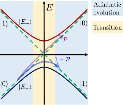
Figure 1: The two-level system and the adiabatic-impulse model. The approximation consists in the assumption that the evolution is described by the alternation of stages. During the adiabatic stages the system follows either a ground state $E_{-}$ or an excited state $E_{+}$. The impulse-type transition (with the probability $\mathcal{P}$) is assumed to happen in the point of the minimal energy-level splitting. In this work, the adiabatic-impulse model is justified within Majorana’s approximation.

However, several important questions are left unanswered. For one thing, “it is interesting to contemplate an ambitious program, where one might infer the time-dependence of states from the time-dependent energy levels” [13]. Does Majorana’s approach give the correct description of the dynamics? And not only the asymptotic behaviour at infinity. Following Refs. [1, 13, 16], we explore in detail Majorana’s approach. Not only we present how to obtain the asymptotic transition probability at infinity, but we also introduce and describe the adiabatic-impulse model and explore the dynamics near the avoided-level crossing.

The energy levels are schematically shown in Fig. 1. Consider a two-level system with states $\left|0\right\rangle$ and $\left|1\right\rangle$. If starting, say, to the left in a ground state (more generally, in a superposition state), what is the transition probability to the excited state to the right? What will be the full wave function far from the avoided-level crossing to the right? The answer to this latter question would help to justify a convenient adiabatic-impulse model. This model assumes that the transition region is considered to be infinitely thin, while elsewhere the evolution is modelled as adiabatic.

The rest of this work is organised as follows. In Sec. II (with details in Appendix A) we follow Majorana’s methodology and, solving the Schrödinger equation, obtain the time-dependent wave function. The asymptotic behaviour of this, at $t\rightarrow\infty$, is further analyzed in Sec. III (with details in Appendix B), resulting in the LZSM transition probability, Stokes phase change, and the convenient adiabatic-impulse model. The solution following Majorana is compared with the one following Zener in Sec. IV (with details in Appendix C). Further developments of the Majorana’s approach are the time evolution in Sec. V and using a superposition initial state in Sec. VI.

Note that the English version of Ref. [1] is available in the book [18] and also in the second edition in Ref. [19], commented by M. Inguscio [20]. For Majorana’s biography and research see Ref. [21] and also the book [22].

II Direct and inverse Laplace transforms

In his work [1], Ettore Majorana studied an oriented atomic beam passing a point of a vanishing magnetic field; the second half of the paper was devoted to a spin-1/2 particle in a linearly time-dependent magnetic field. The author considered the problem about a spin orientation in a dynamic magnetic field with components $H_{x}\sim-\Delta$, $H_{y}=0$, and $H_{z}\sim-vt$, where $\Delta$ and $v$ are constant values.

The time evolution of a linearly driven two-level system is governed by the Schrödinger equation:

$$i\hbar\frac{\partial}{\partial t}\left|\psi\right\rangle=-\frac{1}{2}\left(\Delta\sigma_{x}+vt\sigma_{z}\right)\left|\psi\right\rangle,$$ (1)

where $\sigma_{i}$ are the Pauli matrices.

For the wave function in the form

$$\left|\psi\right\rangle=\begin{pmatrix}\alpha\\ \beta\end{pmatrix}$$ (2)

this can be rewritten as a system of two coupled ordinary differential equations. Introducing the dimensionless time $\tau$ and the adiabaticity parameter $\delta$

$$\tau=\sqrt{\frac{v}{2\hbar}}t\text{, \ \ }\delta=\frac{\Delta^{2}}{4v\hbar},$$ (3)

and making the substitutions

$$\alpha=f\exp\!{\left(\frac{i}{2}\tau^{2}\right)},\text{ }\beta=g\exp\!{\left(-\frac{i}{2}\tau^{2}\right)},$$ (4)

we obtain

$$\begin{cases}\dot{f}\!&=i\sqrt{2\delta}g\exp{(-i\tau^{2}),}\\ \dot{g}\!&=i\sqrt{2\delta}f\exp{(i\tau^{2}).}\end{cases}$$ (5)

These can be rewritten for $f$ and $g$ separately

$$\frac{d^{2}f}{d\tau^{2}}+2i\tau\frac{df}{d\tau}+2\delta f = 0,$$ (6)

$$\frac{d^{2}g}{d\tau^{2}}-2i\tau\frac{dg}{d\tau}+2\delta g = 0.$$ (7)

The substitution (4) is used for obtaining these equations in homogeneous form. In this form the Laplace transform simplifies the equations. (Note that to obtain Majorana’s equations we have to replace $\tau\rightarrow\sqrt{2}\tau_{\mathrm{M}}$ and $\sqrt{\delta}\rightarrow-\sqrt{k}/2$, where $\tau_{\mathrm{M}}$ and $k$ is Majorana’s notation.) Following Majorana, the equation for $f(\tau)$, Eq. (6), can be solved by the two-sided Laplace transform,

$$\mathcal{L}[f(\tau)]=\int_{-\infty}^{\infty}\!\!\!e^{-s\tau}f(\tau)\;d\tau=F(s).$$ (8)

Here $F(s)$ is the Laplace transform of the function $f(\tau)$. Then we substitute this in Eq. (6), use the theorem about differentiation of the original function,
$\mathcal{L}[\tau f(\tau)]=-F^{\prime}(s)$, and obtain

$$s^{2}F(s)-2i\left[F(s)+sF^{\prime}(s)\right]+2\delta F(s)=0.$$ (9)

The solution of this first-order differential equation gives

$$F(s)=C_{\delta}\exp{\left(-\frac{is^{2}}{4}\right)}s^{-1-i\delta}.$$ (10)

Here the constant of integration $C_{\delta}$ could be defined from an initial condition. And then we can find $f(\tau)$ from the inverse Laplace transform:

$$f(\tau)=\lim_{T\rightarrow\infty}\int_{\gamma-iT}^{\gamma+iT}e^{s\tau}F(s)\;ds,$$ (11)

where $\gamma$ is a real number so that the contour path of integration is in the region of convergence of $F(s)$. This integral can be calculated by the steepest descent method [23]. For the following calculations, the contour could be deformed due to the residue theorem. This requires large times and we need to find the solution in two limits: for large positive time, which means that $\tau\rightarrow+\infty$, and for large negative time $\tau\ll 0$. Then, the integration contour in Eq. (11) is over either the contour $L_{1}$ for $\tau<0$ or $L_{2}$ for $\tau>0$, the contours to be defined. How the contours are chosen is described in detail in Appendix A; these steepest-descent contours $L_{1,2}$ are demonstrated in Fig. 2.

Our integral (11) has two contributions: the first one is from the saddle point and the second one is from the vicinity of zero. Details of the calculations are presented in Appendix A.

First, we can write the contribution from the saddle point for $f(\tau)$ as follows

$$f(\tau)=C_{\delta}\sqrt{{4\pi}}(-2i\tau)^{-1-i\delta}\exp\!{\left(i\frac{3\pi}{4}-i\tau^{2}\right)}.$$ (12)

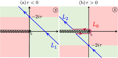
Figure 2: Contours of integration $L_{1,2}$ in Eq. (11) as used in Ref. [1]. The regions where the saddle point method could be applied are shown in green. The contour $L_{1}$ in (a) corresponds to $\tau<0$, and $L_{2}$ in (b) corresponds to $\tau>0$. The contour $L_{0}$ is a part of the contour $L_{2}$, which is partly situated in the red region. The integration along this contour should be calculated separately from the integral calculated within the saddle-point method, both of which contribute to the integral in Eq. (11).

Second, we describe the contribution from the near-zero region $s\rightarrow 0$, which is the integral Eq. (11) on the contour $L_{0}$. Here $L_{0}$ is the near-zero vicinity contour with the neckline along the negative axis which is a part of the $L_{2}$ contour. Here we can neglect the term $s^{2}/4$ next to $s\tau$, and then we use the Gamma function in the Hankel integral representation [24, §12.22]:

$$\int_{L_{0}}e^{x}x^{-y}dx\approx\frac{2\pi i}{\Gamma(y)}.$$ (13)

For using this, we define the replacement $x=s\tau$ and then for the integral in Eq. (11) we have

$$\int_{L_{0}}\tau^{i\delta}\frac{e^{x}}{x^{1+i\delta}}dx=\tau^{i\delta}\frac{2\pi i}{\Gamma(1+i\delta)}.$$ (14)

So, we obtain the approximate solution of Eq. (6) for two cases, $\tau<0$ and $\tau>0$, in the general form. The second part of the spinor, $g(\tau)$, is obtained from Eq. (5) neglecting the terms $\sim\tau^{-2}$ because this result is asymptotic. Then using the substitutions Eq. (4), we obtain

$$\tau<0:\begin{cases}\alpha(\tau)=C_{\delta}\sqrt{4\pi}(-2i\tau)^{-i\delta-1}\exp\!\left(-i\frac{\tau^{2}}{2}+i\frac{3\pi}{4}\right),\\ \beta(\tau)=C_{\delta}\sqrt{\frac{2\pi}{\delta}}(-2i\tau)^{-i\delta}\exp\!\left(-\frac{i\tau^{2}}{2}+\frac{i\pi}{4}\right),\end{cases}$$ (15a)

$$\tau>0:\begin{cases}\alpha(\tau)=C_{\delta}\sqrt{4\pi}(-2i\tau)^{-i\delta-1}\exp\!\left(-\frac{i\tau^{2}}{2}+i\frac{3\pi}{4}\right)+C_{\delta}\frac{2\pi i}{\Gamma(i\delta+1)}\tau^{i\delta}\exp\!\left(\frac{i\tau^{2}}{2}\right),\\ \beta(\tau)=C_{\delta}\sqrt{\frac{2\pi}{\delta}}(-2i\tau)^{-i\delta}\exp\!\left(-\frac{i\tau^{2}}{2}+\frac{i\pi}{4}\right)+C_{\delta}\sqrt{\frac{\delta}{2}}\frac{2\pi i}{\Gamma(i\delta+1)}\tau^{i\delta-1}\exp\!\left(\frac{i\tau^{2}}{2}\right).\end{cases}$$ (15b)

We now consider the initial condition far from the avoided-level crossing, at $\tau\rightarrow-\infty$, and from Eq. (15a) obtain

$$\begin{cases}|\alpha|^{2}=0\\ |\beta|^{2}=1\end{cases}.$$ (16)

To fulfil the normalization condition we have taken the constant of integration $C_{\delta}$ as

$$C_{\delta}=\sqrt{\frac{\delta}{2\pi}}e^{-\frac{\pi\delta}{2}},$$ (17)

where we used that $i^{i\delta}=e^{-\pi\delta/2}$. Note that the initial condition (16) leaves the phase undefined, so that replacing $C_{\delta}\rightarrow C_{\delta}e^{i\vartheta}$ with any phase $\vartheta~{}$would result in the same initial condition.

III Probability, phase, and adiabatic-impulse model

III.1 Asymptotic solution

Based on the general equations above, we consider the limiting case. Omitting the terms $\sim\tau^{-1}$, from Eq. (15), we obtain the asymptotes for $\alpha(\tau)$ and $\beta(\tau)$

$$\alpha(\tau\rightarrow-\infty)\rightarrow 0,$$ (18)

$$\beta(\tau\rightarrow-\infty)\rightarrow\left(-2i\tau\right)^{-i\delta}\exp\!\left(\frac{i\pi}{4}-\frac{\pi\delta}{2}-\frac{i\tau^{2}}{2}\right),$$

$$\alpha(\tau\rightarrow\infty)\rightarrow\frac{\sqrt{2\pi\delta}}{\Gamma(1+i\delta)}\tau^{i\delta}\exp\!{\left(-\frac{\pi\delta}{2}+\frac{i\pi}{2}+\frac{i\tau^{2}}{2}\right)},$$

$$\beta(\tau\rightarrow\infty)\rightarrow\left(-2i\tau\right)^{-i\delta}\exp\!\left(\frac{i\pi}{4}-\frac{\pi\delta}{2}-\frac{i\tau^{2}}{2}\right).$$

The expressions for $\beta(\tau)$ before and after the transition are similar. It is important to note that according to the sign of $\tau$ these formulas have different absolute values far from the transition region. When $\tau<0$, we see that the expression ibecomes

$$\beta(\tau\rightarrow-\infty)\rightarrow\left(2|\tau|\right)^{-i\delta}\exp\!\left(\frac{i\pi}{4}-\frac{i\tau^{2}}{2}\right),$$ (19)

the absolute value of this is 1. However, when $\tau>0$ the result is

$$\beta(\tau\rightarrow\infty)\rightarrow\left(2|\tau|\right)^{-i\delta}\exp\!\left(-\pi\delta+\frac{i\pi}{4}-\frac{i\tau^{2}}{2}\right),$$ (20)

then the absolute value of this expression is different from $1$. The respective transition probability is

$$\mathcal{P}=\left|\beta(\tau\rightarrow\infty)\right|^{2}=\exp\left[-2\pi\delta\right].$$ (21)

This is known as the LZSM formula. In view that many (if not most) authors in this context refer to this as the LZ formula, we emphasize that Majorana published this very result in Ref. [1] before LZS  [2, 3, 4, 5].

Being interested not only in the transition probability but rather in finding the full wave function, including the phase, we rewrite Eq. (18) in the exponential form:

$$\alpha(\tau\rightarrow\infty)\!\! \approx \!\!\sqrt{1-\mathcal{P}}\exp\left[i\mathrm{Arg}\left[\Gamma(1-i\delta)\right]+\frac{i\tau^{2}}{2}+i\delta\ln{\tau}\right]\!\!,$$

$$\beta(\tau\rightarrow\infty)\! \approx \!\sqrt{\mathcal{P}}\exp\left[\frac{i\pi}{4}-\frac{i\tau^{2}}{2}-i\delta\ln{2\tau}\right]\!.$$ (22)

Interestingly, in [1], Majorana obtained only the correct probability, Eq. (21). The phase in Eq. (22) can be obtained from Majorana’s formulas if we note that there is a typo in the result for function $f(\tau\rightarrow\infty)$ in Ref. [1]: we should correct the typo by replacing

$$e^{-k/4i}\rightarrow\tau_{\mathrm{M}}^{-k/4i},$$ (23)

and we have also to replace $\sqrt{k}\rightarrow-2\sqrt{\delta}$ and $\tau_{\mathrm{M}}\rightarrow\tau/\sqrt{2}$ to obtain our Eq. (22).

III.2 Adiabatic-impulse model

Let us further extend our results above by introducing the adiabatic-impulse model [25, 26, 10]. In brief, this model consists of adiabatic evolution far from the avoided-level crossing, described by the propagators $U_{\mathrm{ad}}$ and the impulse-type probabilistic transition in the point of the avoided-level crossing, see Fig. 1. The latter is described by the matrix $N$, and we will demonstrate now how to obtain this. Far from the quasicrossing point, the evolution could be described in the following way

$$\left|\psi_{\mathrm{f}}\right\rangle=U_{\mathrm{ad}}(0,t_{\mathrm{f}})NU_{\mathrm{ad}}(t_{\mathrm{i}},0)\left|\psi_{\mathrm{i}}\right\rangle,$$ (24)

where $\psi_{\mathrm{i}}$ is the initial wave function with components given by Eq. (18) when $-\tau\rightarrow\infty$, and $\psi_{\mathrm{f}}$ is the final state with components given by Eq. (18) when $\tau_{\mathrm{M}}\rightarrow\infty$. The adiabatic evolution is described in Appendix B.

III.3 Non-adiabatic transition

A non-adiabatic transition is described by the transfer matrix, which is associated with a scattering matrix [27] in scattering theory. (Note the analogy with Mach-Zehnder interferometer [28, 29, 30].) The components of the transfer matrix are related to the amplitudes of the respective states of the system in energy space. The diagonal elements correspond to the square root of the reflection coefficient $R$, and the off-diagonal elements correspond to the square root of the transmission coefficient $T$ and its complex conjugate:

$$N=\left(\begin{array}[]{cc}\sqrt{R}&\sqrt{T}\\ -\sqrt{T}^{\ast}&\sqrt{R}\end{array}\right).$$ (25)

In our problem we obtain for the diagonal from Eqs. (18) elements

$$R=\mathcal{P}\text{ \ \ and \ \ }T=(1-\mathcal{P})\exp\left(i2\varphi_{\mathrm{S}}\right),$$ (26)

where $\varphi_{\mathrm{S}}$ is the Stokes phase

$$\varphi_{\mathrm{S}}=\frac{\pi}{4}+\mathrm{Arg}\left[\Gamma\left(1-i\delta\right)\right]+\delta\left(\ln{\delta}-1\right).$$ (27)

To conclude this section, an avoided-level crossing is described by the adiabatic-impulse model. With the matrices $U$ and $N$, it is straightforward to generalize the model to multi-level systems, e.g. Ref. [31]. This demonstrates the thesis of Ref. [13] that “Majorana’s method is very well adapted to generalizations involving multiple level crossings.”

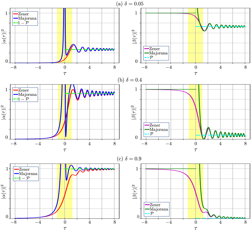
Figure 3: Comparison of the dynamics of the occupation probability versus time $\tau$, obtained by Majorana’s method and Zener’s method. The left panels show the dynamics of the first component of the spinor $\alpha(\tau)$, while the right panels show the second component $\beta(\tau)$, for three different values of the adiabaticity parameter $\delta$. The yellow regions show the area where Majorana’s approach does not give the correct result because that method is asymptotic. The bright green dashed lines show the LZSM probability. These illustrate that far from the transition region both results, by Zener and Majorana, tend to that value.

IV Comparison with Zener’s approach

As we wrote in the Introduction, out of the four approaches by LZSM [1, 2, 3, 4, 5], the total wave function is given only by the approaches by Zener and Majorana. The former is well known, while the latter is examined and extended here. Let us now compare the results by these two approaches.

For readers’ convenience, we write down here the final formulas of the Zener’s approach (for details, see Ref. [8] and references therein):

$$\alpha = A_{+}D_{-1-i\delta}\left(z\right)+A_{-}D_{-1-i\delta}\left(-z\right),$$ (28)

$$\beta = B_{+}D_{-i\delta}\left(z\right)+B_{-}D_{-i\delta}\left(-z\right).$$

Here $z=\tau\sqrt{2}e^{i\pi/4}$, $D_{\nu}(z)$ is the parabolic cylinder function, $B_{\pm}=\mp\delta^{-1/2}\exp{\left(-i\pi/4\right)}A_{\pm}$, and the coefficients $A_{\pm}$ are defined from an initial condition. We aim to compare the results obtained within Zener’s approach with the ones obtained here employing Majorana’s approach, Eq. (15). For this we need to use the asymptotic behavior of a full analytical solution, see Appendix C, and apply the initial condition Eq. (16). As an impressive result, the asymptotic expressions for the wave function by Zener, coincide with the ones we derived in Eq. (15) extending Majorana’s approach.

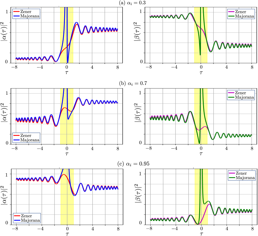
Figure 4: Time-evolution of the occupation probability when starting from different initial superposition states. Similarly to Fig. 3, we present the comparison of the dynamics obtained by following Majorana’s method and Zener’s method, now for three different initial states, with $\alpha_{\mathrm{i}}=0.3$, $0.7$, and $0.95$; $\beta_{\mathrm{i}}=\sqrt{1-\alpha_{\mathrm{i}}^{2}}$. The adiabaticity parameter here is $\delta=0.1$.

V Dynamics

For describing the dynamics of quantum systems, it is necessary to know the behaviour of the wave function for all times. Majorana obtained only the probability of the transition from the ground state to the excited one. We expand Majorana’s method and obtain the dynamics of the wave function. Still, this method is asymptotic, and it is expected not to work appropriately at small absolute values of the dimensionless time $\tau$. Does this give the correct behaviour at finite values of time? Let us explore this and consider this dynamics, by plotting the energy-level occupations, given by Eqs. (15), as functions of time.

In Fig. 3 we show the occupations of the two levels for the asymptotic result of Majorana’s approach, Eq. ​(15), and the exact result of Zener’s approach, Eq. ​(28). As a nice surprise, Fig. 3 shows that the asymptotic solution correctly describes the dynamics at $\left|\tau\right|\gtrsim 1$; and this means that, even for relatively small times, Majorana’s approach gives correct results. Thus, Majorana’s approach not only describes correctly the asymptotic values at infinity (which was the subject of Sec. III), but also the transient dynamics. Only in the very vicinity of zero, when $\left|\tau\right|\lesssim 1$, the asymptotic solution does not work correctly. As shown in Fig. 3, this region, shown by the yellow background colour, is rather narrow.

Let us quantify the region where our Majorana-type solution, Eq. (15), significantly deviates from the exact solution. As we can see from Fig. 3, this time interval corresponds to the so-called jump time [32, 8]. The jump time could be defined via the derivative at zero time, $P^{\prime}(0)$, in the following way for the Zener’s approach

$$\tau_{\mathrm{jump}}=\frac{1-\mathcal{P}}{P^{\prime}(0)},$$ (29)

where $P(\tau)$ is the time-dependent transition probability from the lower level to the upper one. We obtain this probability as $P(\tau)=|\alpha(\tau)|^{2}$ from Eq. (28) using the initial condition Eq. (16)

$$P(\tau)=\delta\exp{\left(-\frac{\pi\delta}{4}\right)}\left|D_{-i\delta-1}(-z)\right|^{2}.$$ (30)

Then the jump time depends on the adiabaticity parameter $\delta$ as follows

$$\tau_{\mathrm{jump}}(\delta)=\frac{\sqrt{1-\mathcal{P}}}{\sqrt{2\delta}\cos\chi(\delta)},$$ (31)

where

$$\chi(\delta)=\frac{\pi}{4}+\mathrm{Arg}\left[\Gamma\left(\frac{1}{2}-\frac{i\delta}{2}\right)\right]-\mathrm{Arg}\left[\Gamma\left(1-\frac{i\delta}{2}\right)\right].$$ (32)

Based on this formula, we can analytically estimate the area where our method does not give the correct result: the width of the yellow-background area in Fig. 3 corresponds to $\tau_{\mathrm{jump}}$, given by Eq. (31).

VI Arbitrary initial state

When in Sec. II we solved the evolution equations following Majorana, we obtained the specific initial condition, Eq. (16). If one is interested in any other initial condition, this solution is invalid. This is because this approach gives a partial solution of Eq. (6). In order to find the general solution, we need to obtain a second partial solution, linearly independent from the first one. This we can obtain by solving Eq. (7) analogously to how we did in Sec. II. Let us call these two solutions $\left|\psi_{1}\right\rangle$ and $\left|\psi_{2}\right\rangle$ with

$$\left|\psi_{1,2}\right\rangle=\begin{pmatrix}\alpha_{1,2}\\ \beta_{1,2}\end{pmatrix}.$$ (33)

Instead of solving Eq. (7), we note that this coincides with Eq. (6) by swapping $\alpha_{2}$ with $\beta_{1}$ and $\beta_{2}$ with $\alpha_{1}$ and taking their complex conjugate, with the appropriate choice of the branch in the square root. In the method of steepest descent, the branch depends on the inclination angle of the integration contour. In the two partial solutions, the inclinations are different, so the branches are also chosen to be different.

Then the general solution is a linear combination of these two solutions, $\left|\psi(\tau)\right\rangle=Q_{1}\left|\psi_{1}(\tau)\right\rangle+Q_{2}\left|\psi_{2}(\tau)\right\rangle$. If we consider a given initial state

$$\left|\psi(\tau_{\mathrm{i}})\right\rangle=\begin{pmatrix}\alpha_{{}_{\mathrm{i}}}\\ \beta_{{}_{\mathrm{i}}}\end{pmatrix},$$ (34)

then the constants are $Q_{1}=\beta_{\mathrm{i}}$ and $Q_{2}=\alpha_{\mathrm{i}}$.

To summarize, the general solution is

$$\left|\psi(\tau)\right\rangle=\beta_{\mathrm{i}}\left|\psi_{1}(\tau)\right\rangle+\alpha_{\mathrm{i}}\left|\psi_{2}(\tau)\right\rangle,$$ (35)

with $\left|\psi_{1}(\tau)\right\rangle$ given by Eq. (15) and $\left|\psi_{2}(\tau)\right\rangle$ obtained from $\left|\psi_{1}(\tau)\right\rangle$ by swapping $\alpha$ and $\beta$ and a subsequent complex conjugation.

Results of calculations for superposition initial states are shown in Fig. 4. There we consider three initial states, when the probability of the $\psi_{1}$-state, which is $\left|\alpha_{\mathrm{i}}\right|^{2}$, is close to $0.1$ (top panel), $0.5$ (middle panel), and $0.9$ (bottom panel). The top panel describes the slight deviation from Majorana’s solution $\left|\psi_{1}\right\rangle$, presented in Fig. 3, while the bottom panel describes the opposite case (which can be called anti-Majorana solution), when the solution is closer to $\left|\psi_{2}\right\rangle$.

Figure 5 shows the validity of our results obtained for a ground (a) and superposition state (b) within Majorana’s approach. This is quantified as the relative difference between our asymptotic solution and the exact one obtained within Zener’s approach. For illustrative purposes we choose the equally populated superposition at the initial time. If $\left|\alpha_{\mathrm{i}}\right|^{2}<0.5$, the figure becomes less symmetric and skewed to the left; if $\left|\alpha_{\mathrm{i}}\right|^{2}>0.5$ then skewed to the right. In addition, we plot dashed blue lines, showing the jump time from Eq. (29), which gives a good estimate of where the asymptotic solution is in agreement with the exact one (outside of the region between the blue curves). Note that the jump-time is not symmetric around the point $\tau=0$. In general, it is asymmetric, and shift relates to the value of the adiabaticity parameter $\delta$.

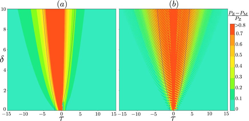
Figure 5: Validity of Majorana’s approach. This is quantified as the difference of the upper-level occupation probability calculated by both the asymptotic Majorana’s method and the exact Zener’s result. The initial condition is taken to be the ground state with $\alpha_{\mathrm{i}}=0$ (a) and the superposition state (b) with $\alpha_{\mathrm{i}}=0.7$. Here $P_{\mathrm{Z}}$ is Zener’s probability which is given by $|\alpha(\tau)|^{2}$ from Eq. (28). Then $P_{\mathrm{M}}$ is our result within Majorana’s approach which is provided by $|\alpha(\tau)|^{2}$ from Eq. (35). The dashed blue lines show the jump time $\tau_{\mathrm{jump}}$, Eq. (29). In general, the jump time is not symmetric around the point $\tau=0$; on the left panel the jump time is shifted to the left, for illustrative purposes.

VII Conclusions

We studied the approach by Majorana to the problem of a transition through a region where the energy levels experience avoided-level crossing. We demonstrated that “Majorana’s method is smooth and capable of considerable generalization” [13], and we considered this here in detail. We obtained in a mathematically elegant way, the asymptotic formulas for the amplitude and phase of the two-level system wave function after a single passage with linear excitation. This was done using Laplace transformations and contour integration. Our study demonstrates that Majorana’s approach justifies the adiabatic-impulse model. We demonstrated that this asymptotic model provides a very good description of the dynamics.

Appendix A Integration contours

We can use the saddle-point method for obtaining the result of the inverse Laplace transform, because our integrals are Laplace-type integrals [23]

$$I(\tau)=\int\limits_{L}\phi(z)\;e^{\tau\mu(z)}dz.$$ (36)

First, we must define the integration contours. These should be situated in the holomorphic region of the sub-integral function. The function $F(s)$ contains an exponential factor, which means that we should define the holomorphy region for a logarithm. This region is the whole complex plane with a cut along the real axis from minus infinity to zero.

The contour $L$ should be a steepest-descent contour of an integral for applying the saddle-point method. For this, the following conditions should be satisfied [23]:
1. There is a point $z_{0}$ belonging to the contour $L$ such that $\mbox{Re}\left[\mu(z_{0})\right]=\max\limits_{z\in L}\mbox{Re}\left[\mu(z)\right]$, where the function $\mu(\tau)$ was defined in the integral Eq. (36);
2. There is such a value $\tau_{0}>0$ that the following integral has a finite value when integrated over the contour $L$

$$\int\limits_{L}|\phi(z)|\exp\left[\tau_{0}\mbox{Re}\mu(z)\right]dz<\infty;$$ (37)

3. For a function $\mu(\tau)$ the following conditions are satisfied:

$$\mu^{\prime}(z_{0}) = 0,$$ (38)

$$\mu^{\prime\prime}(z_{0}) \neq 0,$$

$$\frac{d^{2}}{dy^{2}}\left[\mbox{Re}\mu(z_{0}+y\lambda)\right] = \mathrm{Const}<0,$$

where $\lambda$ is any tangent to contour $L$ in the point $z_{0}$;
4. Functions $\phi$ and $\mu$ are holomorphic in the vicinity of the contour.

The saddle-point method implies that if the contour $L$ is a steepest-descent contour for $I(\tau)$, then

$$I(\tau)=\sqrt{\frac{2\pi}{\tau}}\frac{\phi(z_{0})e^{\tau\mu(z_{0})}}{\sqrt{-\mu^{\prime\prime}(z_{0})}}\left(1+o(1)\right).$$ (39)

A branch of a square root $\sqrt{-\mu^{\prime\prime}(z_{0})}$ should be chosen corresponding to the angle of inclination of the integration contour. We should make a substitution for working with the steepest-descent contour in our problem

$$s=\tau z,\text{ \ \ }ds=\tau dz;$$ (40)

then

$$f(\tau)=C_{\delta}\tau^{-i\delta}\int\limits_{L}\exp\left\{\tau^{2}\left(z-i\frac{z^{2}}{4}\right)\right\}z^{-(i\delta+1)}dz,$$ (41)

$$\phi(z)=z^{-(i\delta+1)},$$ (42)

$$\mu(z)=z-i\frac{z^{2}}{4}.$$ (43)

From the condition #$3$ listed above, we obtain the point $z_{0}$

$$z_{0}=-2i\;\;\Rightarrow\;\;s_{0}=-2i\tau.$$ (44)

Also, we can obtain the angle of inclination of the tangent from the second part of the condition #$3$:

$$\mathrm{Re}\left(-\lambda^{2}\frac{i}{2}\right)<0\;\;\Rightarrow\;\;\mathrm{Arg}\lambda=\frac{3\pi}{4}.$$ (45)

From the condition #$1$ above we obtain the regions where the saddle-point method could be applied, defined by

$$\mathrm{Re}\left[\mu(z_{0})\right]-\mathrm{Re}\left[\mu(z)\right]>0.$$ (46)

The regions corresponding to this condition are highlighted by the light-green colour background in Fig. 2. We need to consider two different contours: with $\tau>0$ and $\tau<0$. In case of $\tau>0$, there is a part of the contour which lays outside of the green area. According to it, in this case the result comes not only from the saddle-point method but also from the integration near the zero point.

Appendix B Adiabatic evolution

In this section we discuss the adiabatic evolution in the diabatic basis. This is needed for the adiabatic-impulse model, which we formulate and justify in Sec. III. Here, the adiabatic evolution consists in staying in one of the adiabatic eigenstates $\left|\varphi_{\pm}(t)\right\rangle$, which are defined as eigenstates of $H(t)$,

$$H(t)\left|\varphi_{\pm}(t)\right\rangle=E_{\pm}(t)\left|\varphi_{\pm}(t)\right\rangle.$$ (47)

Solving the non-stationary Schrödinger equation, $i\hbar\dot{\left|{\psi}\right\rangle}=E\left|\psi\right\rangle$, we obtain [10]

$$\left|\varphi_{\pm}(t)\right\rangle=\left|\varphi_{\pm}(t_{\mathrm{i}})\right\rangle\exp{\left\{\mp i\left(\zeta+\frac{\pi}{4}\right)\right\}},$$ (48)

$$\zeta=\frac{1}{2\hbar}\int_{t_{\mathrm{i}}}^{t}{\Delta E(t^{\prime})dt^{\prime}},$$ (49)

$$\Delta E(t)=E_{+}(t)-E_{-}(t)=\sqrt{\Delta^{2}+\varepsilon^{2}(t)}.$$ (50)

The full wave function is

$$\left|\psi(t)\right\rangle=b_{+}(t)\left|\varphi_{+}(t_{\mathrm{i}})\right\rangle+b_{-}(t)\left|\varphi_{-}(t_{\mathrm{i}})\right\rangle,$$ (51)

where $b_{\pm}$ are the respective amplitudes. In the adiabatic basis we can write the wave function as a vector

$$\left|\psi(t)\right\rangle=\left(\begin{array}[]{c}b_{+}(t)\\ b_{-}(t)\end{array}\right).$$ (52)

This allows us to describe the adiabatic evolution from the time moment $t_{\mathrm{i}}$ to $t_{\mathrm{f}}$ with the evolution matrix $U_{\mathrm{ad}}$:

$$\left(\begin{array}[]{c}b_{+}(t_{\mathrm{f}})\\ b_{-}(t_{\mathrm{f}})\end{array}\right)=U_{\mathrm{ad}}\left(\begin{array}[]{c}b_{+}(t_{\mathrm{i}})\\ b_{-}(t_{\mathrm{i}})\end{array}\right).$$ (53)

The adiabatic evolution is then obtained from Eqs. (52) and (48):

$$U_{\mathrm{ad}}=\left(\begin{array}[]{cc}\exp\left(-i\zeta\right)&0\\ 0&\exp\left(i\zeta\right)\end{array}\right).$$ (54)

In our problem the bias is linear in time $\varepsilon(t)=vt$ and we can calculate the asymptotic expressions for $\zeta$ at large times, i.e. at $t=\pm\tau_{\mathrm{a}}\sqrt{2\hbar/v}$, with $\tau_{\mathrm{a}}\gg 1$:

$$\zeta\left(\pm\tau_{\mathrm{a}}\right) = \frac{1}{2\hbar}\int\limits_{0}^{\pm\tau_{\mathrm{a}}}\sqrt{\Delta^{2}+\varepsilon^{2}}d\tau\approx$$ (55)

$$\approx \pm\left[\frac{\tau_{\mathrm{a}}^{2}}{2}+\frac{\delta}{2}-\frac{\delta}{2}\ln{\delta}+\delta\ln{\sqrt{2}\tau_{\mathrm{a}}}\right].$$ (56)

The diabatic states $\left|\psi_{\pm}\right\rangle$ are the eigenstates of the Hamiltonian with $\Delta=0$, which means

$$\sigma_{z}\left|\psi_{\pm}\right\rangle=\pm\left|\psi_{\pm}\right\rangle\text{.}$$ (57)

We work in the diabatic basis so we need to transfer the adiabatic evolution matrix from the adiabatic basis to the diabatic one. The relation between the bases is [10]

$$\left|\varphi_{\pm}(t)\right\rangle=\gamma_{\mp}\left|\psi_{+}\right\rangle\mp\gamma_{\pm}\left|\psi_{-}\right\rangle,$$ (58)

where

$$\gamma_{\pm}=\frac{1}{\sqrt{2}}\sqrt{1\pm\frac{\varepsilon(t)}{\Delta E(t)}}.$$ (59)

This relation can be simplified far from the transition region, at $|\tau|\gg 1$. Then, the adiabatic evolution matrix in the diabatic basis has two different forms, before the transition,

$$\tau<0:\,\,\,\,U_{\mathrm{ad}}(\tau_{\mathrm{i}},0)=\left(\begin{array}[]{cc}\exp\left(-i\zeta\right)&0\\ 0&\exp\left(i\zeta\right)\end{array}\right)$$ (60)

and after it,

$$\tau>0:\,\,\,\,U_{\mathrm{ad}}(0,\tau_{\mathrm{f}})=\left(\begin{array}[]{cc}\exp\left(i\zeta\right)&0\\ 0&\exp\left(-i\zeta\right)\end{array}\right).$$ (61)

Then the matrix for the overall evolution in the diabatic basis is described by the following matrix

$$U_{\mathrm{ad}}(0,\tau_{\mathrm{f}})NU_{\mathrm{ad}}(\tau_{\mathrm{i}},0)=\begin{pmatrix}\sqrt{R}&\sqrt{T}e^{2i\zeta(\tau_{a})}\\ -\sqrt{T}^{\ast}e^{-2i\zeta(\tau_{a})}&\sqrt{R}\end{pmatrix}.$$ (62)

Appendix C Asymptotics of Zener’s wave function

Zener’s approach gives the full analytical solution in terms of the parabolic cylinder functions, e.g. [8],

$$\begin{cases}\alpha=A_{+}D_{-i\delta-1}(z)+A_{-}D_{-i\delta-1}(-z),\\ \beta=-\frac{A_{+}}{\sqrt{\delta}}\exp\!\left(-i\frac{\pi}{4}\right)\!D_{-i\delta}(z)+\frac{A_{-}}{\sqrt{\delta}}\exp\!\left(-i\frac{\pi}{4}\right)\!D_{-i\delta}(-z),\end{cases}$$ (63)

where $z=\tau\sqrt{2}e^{\frac{i\pi}{4}}$. The coefficients are obtained from an initial condition at $z=z_{\text{i}}$,

$$A_{+} = \frac{\Gamma(1+i\delta)}{\sqrt{2\pi}}\left[\alpha(z_{\text{i}\!\!}\ )D_{-i\delta}(-z_{\text{i}})-\right.$$ (64)

$$\left.-\beta(z_{\text{i}\!\!}\ )e^{i\frac{\pi}{4}}\sqrt{\delta}D_{-1-i\delta}(-z_{\text{i}})\right],$$

$$A_{-} = \frac{\Gamma(1+i\delta)}{\sqrt{2\pi}}\left[\alpha(z_{\text{i}\!\!}\ )D_{-i\delta}(z_{\text{i}})+\right.$$ (65)

$$\left.+\beta(z_{\text{i}\!\!}\ )e^{i\frac{\pi}{4}}\sqrt{\delta}D_{-1-i\delta}(z_{\text{i}})\right].$$

Comparing the time evolution obtained in our work following Majorana’s approach, Eq. (15), with Zener’s wave function requires to take the asymptotic expressions of these formulas. The asymptotes of the parabolic cylinder function are as follows (from Ref. [33]), depending on $\mathrm{Arg}{z}$,

1) for $-\frac{5\pi}{4}<\mathrm{Arg}{z}<-\frac{\pi}{4}$

$$D_{p}(z)\sim\exp{\left(-\frac{z^{2}}{4}\right)}z^{p}-\frac{\sqrt{2\pi}}{\Gamma(-p)}e^{-ip\pi}\exp{\left(\frac{z^{2}}{4}\right)}z^{-p-1}$$ (66)

2) and for $|\mathrm{Arg}z|<\frac{3\pi}{4}$

$$D_{p}(z)\sim\exp{\left(-\frac{z^{2}}{4}\right)}z^{p}.$$ (67)

There are two cases. For $\tau<0$, we have

$$z=\left(-\left|\tau\right|\right)\sqrt{2}\exp{\left(\frac{i\pi}{4}\right)}=\left|\tau\right|\sqrt{2}\exp{\left(-\frac{i3\pi}{4}\right)}$$ (68)

and then Eq. (66) applies. For $\tau>0$ we have

$$z=\tau\sqrt{2}\exp{\left(\frac{i\pi}{4}\right)},$$ (69)

and then Eq. (67) applies.

Using these asymptotic expressions for Eq. (63), we obtain exactly Eq. (15), which shows that the result using Majorana’s approach provides the very same asymptotic time evolution as the one by Zener’s approach.

References

- Majorana [1932] E. Majorana, “Atomi orientati in campo magnetico variabile,” Il Nuovo Cimento 9, 43 (1932).
- Landau [1932a] L. Landau, “Zur theorie der Energieubertragung,” Phyz. Z. Sowjetunion 1, 88 (1932a).
- Landau [1932b] L. Landau, “Zur theorie der Energieubertragung II,” Phyz. Z. Sowjetunion 2, 46 (1932b).
- Zener [1932] C. Zener, “Non-adiabatic crossing of energy levels,” Proc. R. Soc. A 137, 696 (1932).
- Stückelberg [1932] E. C. G. Stückelberg, “Theorie der unelastischen stösse zwischen atomen,” Helv. Phys. Acta 5, 369 (1932).
- Nakamura [2011] H. Nakamura, Nonadiabatic Transition (World Scientific, 2011).
- Shevchenko [2019] S. N. Shevchenko, Mesoscopic Physics meets Quantum Engineering (World Scientific Pub Co Inc, 2019).
- Ivakhnenko et al. [2022] O. V. Ivakhnenko, S. N. Shevchenko, and F. Nori, “Non-adiabatic Landau-Zener-Stückelberg-Majorana transitions, dynamics, and interference,” arXiv:2203.16348 (2022).
- Landau and Lifshitz [1965] L. D. Landau and E. M. Lifshitz, “Quantum Mechanics, Non‐Relativistic Theory,” (Pergamon Press, Oxford, 1965) Chap. 53 Transition under the action of adiabatic perturbation, pp. 185–187, 2nd ed.
- Shevchenko et al. [2010] S. N. Shevchenko, S. Ashhab, and F. Nori, “Landau–Zener–Stückelberg interferometry,” Phys. Rep. 492, 1 (2010).
- Child [1996] M. S. Child, Molecular Collision Theory, Dover Books on Chemistry Series (Dover Publications, 1996).
- Child [1974] M. S. Child, “On the Stueckelberg formula for non-adiabatic transitions,” Mol. Phys. 28, 495 (1974).
- Wilczek [2014] F. Wilczek, “Majorana and condensed matter physics,” in The Physics of Ettore Majorana: Theoretical, Mathematical, and Phenomenological (Cambridge University Press, 2014) pp. 279–302.
- Giacomo and Nikitin [2005] F. D. Giacomo and E. E. Nikitin, “The Majorana formula and the Landau–Zener–Stückelberg treatment of the avoided crossing problem,” Phys. Usp. 48, 515 (2005).
- Vitanov and Garraway [1996] N. V. Vitanov and B. M. Garraway, “Landau-Zener model: Effects of finite coupling duration,” Phys. Rev. A 53, 4288 (1996).
- Rodionov et al. [2016] Y. I. Rodionov, K. I. Kugel, and F. Nori, “Floquet spectrum and driven conductance in Dirac materials: Effects of Landau-Zener-Stückelberg-Majorana interferometry,” Phys. Rev. B 94, 195108 (2016).
- Dogra et al. [2020] S. Dogra, A. Vepsäläinen, and G. S. Paraoanu, “Majorana representation of adiabatic and superadiabatic processes in three-level systems,” Phys. Rev. Research 2, 043079 (2020).
- Bassani [2006] G. F. Bassani, ed., “Ettore Majorana scientific papers. On occasion of the centenary of his birth,” (Springer, Berlin, 2006) Chap. Oriented atoms in a variable magnetic field, pp. 125–132.
- Cifarelli [2020a] L. Cifarelli, ed., “Scientific Papers of Ettore Majorana,” (Springer, Berlin, 2020) Chap. Oriented atoms in a variable magnetic field, pp. 77–84.
- Cifarelli [2020b] L. Cifarelli, ed., “Scientific Papers of Ettore Majorana,” (Springer, Berlin, 2020) Chap. Comment on: ”Oriented atoms in a variable magnetic field”, by M. Inguscio, pp. 85–88.
- Esposito [2014] S. Esposito, The Physics of Ettore Majorana: Theoretical, Mathematical, and Phenomenological (Cambridge University Press, 2014).
- Esposito [2017] S. Esposito, Ettore Majorana (Springer-Verlag GmbH, 2017).
- Fedoruk [1977] M. Fedoruk, Method of the steepest descent (1977) pp. 162–184.
- Whittaker and Watson [1920] E. T. Whittaker and G. N. Watson, A Course of Modern Analysis, 3rd ed. (Cambridge University Press, 1920) Chap. The parabolic cylinder functions. Weber’s equation, pp. 347–349.
- Damski [2005] B. Damski, “The simplest quantum model supporting the Kibble-Zurek mechanism of topological defect production: Landau-Zener transitions from a new perspective,” Phys. Rev. Lett. 95, 035701 (2005).
- Damski and Zurek [2006] B. Damski and W. H. Zurek, “Adiabatic-impulse approximation for avoided level crossings: from phase-transition dynamics to Landau-Zener evolutions and back again,” Phys. Rev. A 73, 063405 (2006).
- Moskalets [2011] M. V. Moskalets, Scattering matrix approach to non-stationary quantum transport (World Scientific, 2011).
- Oliver et al. [2005] W. D. Oliver, Y. Yu, J. C. Lee, K. K. Berggren, L. S. Levitov, and T. P. Orlando, “Mach-Zehnder interferometry in a strongly driven superconducting qubit,” Science 310, 1653 (2005).
- Sillanpää et al. [2006] M. Sillanpää, T. Lehtinen, A. Paila, Y. Makhlin, and P. Hakonen, “Continuous-time monitoring of Landau-Zener interference in a Cooper-pair box,” Phys. Rev. Lett. 96, 187002 (2006).
- Burkard [2010] G. Burkard, “Splitting spin states on a chip,” Science 327, 650 (2010).
- Suzuki and Nakazato [2022] T. Suzuki and H. Nakazato, “Generalized adiabatic impulse approximation,” Phys. Rev. A 105, 022211 (2022).
- Vitanov [1999] N. V. Vitanov, “Transition times in the Landau-Zener model,” Phys. Rev. A 59, 988 (1999).
- Gradshteyn and Ryzhik [2007] I. S. Gradshteyn and I. M. Ryzhik, “Table of Integrals, Series, and Products,” (Academic Press is an imprint of Elsevier, 2007) Chap. 9, pp. 1028–1031, seventh ed.