Linear quadratic leader-follower stochastic differential games for mean-field switching diffusions

Abstract

In this paper, we consider a linear quadratic (LQ) leader-follower stochastic differential game for regime switching diffusions with mean-field interactions. One of the salient features of this paper is that conditional mean-field terms are included in the state equation and cost functionals. Based on stochastic maximum principles (SMPs), the follower’s problem and the leader’s problem are solved sequentially and an open-loop Stackelberg equilibrium is obtained. Further, with the help of the so-called four-step scheme, the corresponding Hamiltonian systems for the two players are decoupled and then the open-loop Stackelberg equilibrium admits a state feedback representation if some new-type Riccati equations are solvable.

Keywords: leader-follower game, linear quadratic problem, Markov chain, mean-field interaction, Riccati equation

1 Introduction

The leader-follower game involves two players with asymmetric roles, one called the leader and the other called the follower. In the game, the leader first announces her action, and the follower, according to the leader’s action, chooses an optimal response to minimize his cost functional. Next, the leader has to take the follower’s optimal response into account and chooses an optimal action to minimize her cost functional. Yong [32] first considered a linear quadratic (LQ) leader-follower stochastic differential game. Then, within the LQ framework, the result was extended by, e.g., [27, 23, 17] in different settings.

Mean-field stochastic differential equations (SDEs) were initially suggested to describe physical systems involving a large number of interacting particles. In the dynamics of a mean-field SDE, one replaces the interactions of all the particles by their average or mean to reduce the complexity of the problem. In the last decade, since Buchdahn et al. [3, 4] and Carmona and Delarue [5, 6, 7] introduced the mean-field backward SDEs (BSDEs) and mean-field forward-backward SDEs (FBSDEs), optimal control problems, especially stochastic maximum principles (SMPs), for mean-field systems have become a popular topic; see, for example, [16, 33, 30, 9, 10, 8, 36, 19, 1, 29].

Another feature of this paper is the use of a regime switching model, in which the continuous state of the LQ problem and the discrete state of the Markov chain coexist; see [34, 38, 28, 39, 35, 20, 21] for more information and applications of regime switching models. Recently, Nguyen, Yin, and Hoang [25] established the law of large numbers for systems with regime switching and mean-field interactions, where the mean-field limit was characterized as the conditional expectation of the solution to a conditional mean-field SDE with regime switching (see also Remark 2.1). This work paves the way for treating mean-field optimal control problems with regime switching; see [24, 26, 2, 11].

In this paper, we consider an LQ leader-follower stochastic differential game for mean-field switching diffusions. Based on the SMP in Nguyen, Nguyen, and Yin [24], an open-loop optimal control for the follower is obtained. Then, by applying the four-step scheme developed by Ma, Protter, and Yong [22], we derive its (anticipating) state feedback representation in terms of two Riccati equations and an auxiliary BSDE. Knowing the follower’s optimal control, the leader faces a state equation which is a conditional mean-field FBSDE with regime switching. We also utilize the SMP to obtain an open-loop optimal control for the leader. Then, by the dimensional augmentation approach in Yong [32], a non-anticipating state feedback representation is derived in terms of two Riccati equations. As a consequence, the follower’s optimal control can be also represented in a non-anticipating way.

The rest of this paper is organized as follows. In the next, we present an example which motivates us to study the leader-follower problem in this paper. In Section 2, we formulate the problem and provide some preliminary results. In Sections 3 and 4, we solve the LQ problems for the follower and the leader, respectively. Finally, Section 5 concludes the paper.

Motivation: a pension fund optimization problem. Typically, in a defined benefit (DB) scheme pension fund there are two participants who make contributions: one is the leader (such as the company) with contribution rate $u_{2}(\cdot)$, the other one is the follower (such as the individual) with contribution rate $u_{1}(\cdot)$. The dynamics of the pension fund is described as

$$dF(t)=F(t)d\Delta(t)+\{u_{1}(t)+u_{2}(t)-\xi_{0}\}dt,$$

where $d\Delta(t)$ is the return rate of the fund and $\xi_{0}$ is the pension scheme benefit outgo. The pension fund is invested in a bond $S_{0}(t)$ and a stock $S(t)$, which are given by

$$\left\{\begin{aligned} dS_{0}(t)=&r(\alpha(t))S_{0}(t)dt,\\ dS(t)=&b(\alpha(t))S(t)dt+\sigma(\alpha(t))S(t)dW(t),\end{aligned}\right.$$

where $r(i)$ is the interest rate, $b(i)$ is the appreciation rate, and $\sigma(i)$ is the volatility corresponding to the market regime $\alpha(t)=i$. Assume the proportions $\pi(\cdot)$ and $1-\pi(\cdot)$ of the fund are to be allocated in the stock and the bond, respectively. Then we have

$$d\Delta(t)=\{r(\alpha(t))+[b(\alpha(t))-r(\alpha(t))]\pi(t)\}dt+\sigma(\alpha(t))\pi(t)dW(t).$$

Therefore, the dynamics of the pension fund can be written as

$$dF(t)=\{r(\alpha(t)) F(t)+[b(\alpha(t))-r(\alpha(t))]\pi(t)F(t)$$

$$+ u_{1}(t)+u_{2}(t)-\xi_{0}\}dt+\sigma(\alpha(t))\pi(t)F(t)dW(t).$$

The cost functionals for the follower and the leader to minimize are defined as

$$J_{k}(u_{1}(\cdot),u_{2}(\cdot))=\frac{1}{2}E\bigg{[}\int_{0}^{T}\Big{(}u_{k}(t)-\xi_{k}\Big{)}^{2}dt+\Big{(}E[F(T)|\mathcal{F}_{T}^{\alpha}]-\xi_{T}\Big{)}^{2}\bigg{]},\quad k=1,2,$$

respectively, where $\xi_{k}$, $k=1,2$, are the running benchmark, and $\xi_{T}$ is the terminal wealth target; both are introduced to measure the stability and performance of the pension scheme.

The above pension fund optimization problem formulates naturally a special case of the LQ leader-follower game considered in this paper. For more pension fund optimization problems under various contexts, see [12, 14, 37]; for a conditional mean-variance portfolio selection problem (as an application of conditional mean-field control theory), see [26].

2 Problem formulation and preliminaries

Let $R^{n}$ be the $n$-dimensional Euclidean space with Euclidean norm $|\cdot|$ and Euclidean inner product $\langle\cdot,\cdot\rangle$. Let $R^{n\times m}$ be the space of all $(n\times m)$ matrices. $A^{\top}$ denotes the transpose of a vector or matrix $A$. $I_{n}$ denotes the $(n\times n)$ identity matrix.

Let $[0,T]$ be a finite time horizon and $(\Omega,\mathcal{F},P)$ be a fixed probability space on which a one-dimensional standard Brownian motion $W(t)$, $t\in[0,T]$, and a Markov chain $\alpha(t)$, $t\in[0,T]$, are defined. The Markov chain $\alpha(\cdot)$ takes values in a finite state space $\mathcal{M}$. Let $Q=(\lambda_{ij})_{i,j\in\mathcal{M}}$ be the generator (i.e., the matrix of transition rates) of $\alpha(\cdot)$ with $\lambda_{ij}\geq 0$ for $i\neq j$ and $\sum_{j\in\mathcal{M}}\lambda_{ij}=0$ for each $i\in\mathcal{M}$. Assume that $W(\cdot)$ and $\alpha(\cdot)$ are independent. For $t\geq 0$, denote $\mathcal{F}^{\alpha}_{t}=\sigma\{\alpha(s):0\leq s\leq t\}$ and $\mathcal{F}_{t}=\sigma\{W(s),\alpha(s):0\leq s\leq t\}$. Let $\mathcal{L}_{\mathcal{F}}^{2}(R^{n})$ be the set of all $R^{n}$-valued $\mathcal{F}_{t}$-adapted processes $x(\cdot)$ on $[0,T]$ such that $E\int_{0}^{T}|x(t)|^{2}dt<\infty$.

The state of the system is described by the following linear conditional mean-field SDE with regime switching on $[0,T]$:

$$\left\{\begin{aligned} dx(t)=&\Big{[}A(\alpha(t))x(t)+\widehat{A}(\alpha(t))E[x(t)|\mathcal{F}_{t}^{\alpha}]+B_{1}(\alpha(t))u_{1}(t)+B_{2}(\alpha(t))u_{2}(t)\Big{]}dt\\ +&\Big{[}C(\alpha(t))x(t)+\widehat{C}(\alpha(t))E[x(t)|\mathcal{F}_{t}^{\alpha}]+D_{1}(\alpha(t))u_{1}(t)+D_{2}(\alpha(t))u_{2}(t)\Big{]}dW(t),\\ x(0)=&x_{0},\end{aligned}\right.$$ (1)

where $x(\cdot)$ is the state process with values in $R^{n}$, $u_{1}(\cdot)$ and $u_{2}(\cdot)$ are control processes taken by the follower and the leader, with values in $R^{m_{1}}$ and $R^{m_{2}}$, respectively, and $A(i)$, $\widehat{A}(i)$, $B_{1}(i)$, $B_{2}(i)$, $C(i)$, $\widehat{C}(i)$, $D_{1}(i)$, $D_{2}(i)$, $i\in\mathcal{M}$, are constant matrices of suitable dimensions. It follows from Nguyen et al. [24, 26] that, for any $u_{1}(\cdot)\in\mathcal{L}_{\mathcal{F}}^{2}(R^{m_{1}})$ and $u_{2}(\cdot)\in\mathcal{L}_{\mathcal{F}}^{2}(R^{m_{2}})$, SDE (1) admits a unique solution $x(\cdot)\in\mathcal{L}_{\mathcal{F}}^{2}(R^{n})$. Then, $\mathcal{U}_{1}\doteq\mathcal{L}_{\mathcal{F}}^{2}(R^{m_{1}})$ and $\mathcal{U}_{2}\doteq\mathcal{L}_{\mathcal{F}}^{2}(R^{m_{2}})$ are called the admissible control sets for the follower and the leader, respectively.

The cost functionals for the follower and the leader to minimize are defined as

$$J_{k}(u_{1}(\cdot),u_{2}(\cdot))= \frac{1}{2}E\bigg{[}\int_{0}^{T}\bigg{(}\Big{\langle}Q_{k}(\alpha(t))x(t),x(t)\Big{\rangle}+\Big{\langle}\widehat{Q}_{k}(\alpha(t))E[x(t)|\mathcal{F}_{t}^{\alpha}],E[x(t)|\mathcal{F}_{t}^{\alpha}]\Big{\rangle}$$ (2)

$$+\Big{\langle}N_{k}(\alpha(t))u_{k}(t),u_{k}(t)\Big{\rangle}\bigg{)}dt+\Big{\langle}G_{k}(\alpha(T))x(T),x(T)\Big{\rangle}$$

$$+\Big{\langle}\widehat{G}_{k}(\alpha(T))E[x(T)|\mathcal{F}_{T}^{\alpha}],E[x(T)|\mathcal{F}_{T}^{\alpha}]\Big{\rangle}\bigg{]},\quad k=1,2,$$

respectively, where $Q_{k}(i)$, $\widehat{Q}_{k}(i)$, $N_{k}(i)$, $G_{k}(i)$, $\widehat{G}_{k}(i)$, $k=1,2$, $i\in\mathcal{M}$, are constant symmetric matrices of suitable dimensions.

Remark 2.1.

In fact, SDE (1) is obtained as the mean-square limit as $N\rightarrow\infty$ of a system of interacting particles in the following form:

$$\left\{\begin{aligned} dx^{l,N}(t)=&\bigg{[}A(\alpha(t))x^{l,N}(t)+\widehat{A}(\alpha(t))\frac{1}{N}\sum_{l=1}^{N}x^{l,N}(t)+B_{1}(\alpha(t))u_{1}(t)+B_{2}(\alpha(t))u_{2}(t)\bigg{]}dt\\ +\bigg{[}C(&\alpha(t))x^{l,N}(t)+\widehat{C}(\alpha(t))\frac{1}{N}\sum_{l=1}^{N}x^{l,N}(t)+D_{1}(\alpha(t))u_{1}(t)+D_{2}(\alpha(t))u_{2}(t)\bigg{]}dW^{l}(t),\\ x^{l,N}(0)=&x_{0},\quad 1\leq l\leq N,\end{aligned}\right.$$

where $\{W^{l}(\cdot)\}_{l=1}^{N}$ is a collection of independent standard Brownian motions and the Markov chain $\alpha(\cdot)$ serves as a common noise for all particles, which leads to the conditional expectations rather than expectations in (1).

Intuitively, since all the particles depend on the history of $\alpha(\cdot)$, their average and thereby its limit as $N\rightarrow\infty$ should also depend on this process. This intuition has been justified by the law of large numbers established by Nguyen et al. [25, Theorem 2.1], which shows that the joint process $(\frac{1}{N}\sum_{l=1}^{N}x^{l,N}(\cdot),\alpha(\cdot))$ converges weakly to a process $(\mu_{\alpha}(\cdot),\alpha(\cdot))$, where $(\mu_{\alpha}(t),\alpha(t))=(E[x(t)|\mathcal{F}_{t}^{\alpha}],\alpha(t))$, $0\leq t\leq T$, and $x(\cdot)$ is exactly the solution of (1).

Remark 2.2.

Note that the cost functionals $J_{k}$, $k=1,2$, defined by (2) are standard in the LQ mean-field control literature (see [33, 24, 26]) and, if we assume the Assumptions (A1) and (A2) given in Sections 3 and 4 hold, then $J_{k}$ is convex with respect to $u_{k}$, $k=1,2$, respectively. However, for LQ mean-field games of large-population systems, the tracking-type cost functionals where one wants to keep the system states stay as much close as possible to a function of the mean-field term are more frequently adopted (see [15, 18, 10]).

Now we explain the leader-follower feature of the game; see also Yong [32]. In the game, for any $u_{2}(\cdot)\in\mathcal{U}_{2}$ of the leader, the follower would like to choose an optimal control $u_{1}^{*}(\cdot)\in\mathcal{U}_{1}$ so that $J_{1}(u_{1}^{*}(\cdot),u_{2}(\cdot))$ achieves the minimum of $J_{1}(u_{1}(\cdot),u_{2}(\cdot))$ over $u_{1}(\cdot)\in\mathcal{U}_{1}$. Knowing the follower’s optimal control $u_{1}^{*}(\cdot)$ (depending on $u_{2}(\cdot)$), the leader would like to choose an optimal control $u_{2}^{*}(\cdot)\in\mathcal{U}_{2}$ to minimize $J_{2}(u_{1}^{*}(\cdot),u_{2}(\cdot))$ over $u_{2}(\cdot)\in\mathcal{U}_{2}$.

In a more rigorous way, the follower wants to find an optimal map $\Pi_{1}^{*}:\mathcal{U}_{2}\mapsto\mathcal{U}_{1}$ and the leader wants to find an optimal control $u_{2}^{*}(\cdot)\in\mathcal{U}_{2}$ such that

$$\left\{\begin{aligned} J_{1}(\Pi_{1}^{*}[u_{2}(\cdot)](\cdot),u_{2}(\cdot))=&\inf_{u_{1}(\cdot)\in\mathcal{U}_{1}}J_{1}(u_{1}(\cdot),u_{2}(\cdot)),\quad\forall u_{2}(\cdot)\in\mathcal{U}_{2},\\ J_{2}(\Pi_{1}^{*}[u_{2}^{*}(\cdot)](\cdot),u_{2}^{*}(\cdot))=&\inf_{u_{2}(\cdot)\in\mathcal{U}_{2}}J_{2}(\Pi_{1}^{*}[u_{2}(\cdot)](\cdot),u_{2}(\cdot)).\end{aligned}\right.$$

If the above optimal pair $(\Pi_{1}^{*}[\cdot],u_{2}^{*}(\cdot))$ exists, it is called an open-loop Stackelberg equilibrium of the leader-follower stochastic differential game.

Then we present some preliminary results on the martingales associated with a Markov chain, which are needed to establish the conditional mean-field BSDEs with regime switching. For each pair $(i,j)\in\mathcal{M}\times\mathcal{M}$ with $i\neq j$, define $[M_{ij}](t)=\sum_{0\leq s\leq t}1_{\{\alpha(s-)=i\}}1_{\{\alpha(s)=j\}}$ and $\langle M_{ij}\rangle(t)=\int_{0}^{t}\lambda_{ij}1_{\{\alpha(s-)=i\}}ds$, where $1_{A}$ denotes the indicator function of a set $A$. It follows from [24, 26] that the process $M_{ij}(t)\doteq[M_{ij}](t)-\langle M_{ij}\rangle(t)$ is a purely discontinuous and square-integrable martingale with respect to $\mathcal{F}_{t}^{\alpha}$, which is null at the origin. In this sense, $[M_{ij}](t)$ and $\langle M_{ij}\rangle(t)$ are the optional and predictable quadratic variations of $M_{ij}(t)$, respectively. In addition, we denote $M_{ii}(t)=[M_{ii}](t)=\langle M_{ii}\rangle(t)\equiv 0$ for each $i\in\mathcal{M}$.

Let $\mathcal{S}_{\mathcal{F}}^{2}(R^{n})$ be the set of all $R^{n}$-valued $\mathcal{F}_{t}$-adapted càdlàg processes $y(\cdot)$ on $[0,T]$ such that $E\int_{0}^{T}|y(t)|^{2}dt<\infty$. Let $\mathcal{K}_{\mathcal{F}}^{2}(R^{n})$ be the set of all collections of $R^{n}$-valued $\mathcal{F}_{t}$-adapted processes $\{k_{ij}(\cdot)\}_{i,j\in\mathcal{M}}$ on $[0,T]$ such that $\sum_{i,j\in\mathcal{M}}E\int_{0}^{T}|k_{ij}(t)|^{2}d[M_{ij}](t)<\infty$ with $k_{ii}(t)\equiv 0$ for each $i\in\mathcal{M}$. For convenience, we also denote $k(\cdot)=\{k_{ij}(\cdot)\}_{i,j\in\mathcal{M}}$ and

$$\int_{0}^{t}k(s)\bullet dM(s)=\sum_{i,j\in\mathcal{M}}\int_{0}^{t}k_{ij}(s)dM_{ij}(s),\quad k(s)\bullet dM(s)=\sum_{i,j\in\mathcal{M}}k_{ij}(s)dM_{ij}(s).$$

The following two lemmas play an important role in the subsequent analysis. The proof of the first lemma is elementary and the proof of the second one is similar to that of Xiong [31, Lemma 5.4]. For completeness and readers’ convenience, their proofs are provided here.

Lemma 2.3.

For any $\mathcal{F}_{t}$-adapted and square-integrable processes $x(\cdot)$ and $y(\cdot)$, we have

$$E\Big{[}x(t)E[y(t)|\mathcal{F}_{t}^{\alpha}]\Big{]}=E\Big{[}E[x(t)|\mathcal{F}_{t}^{\alpha}]y(t)\Big{]}=E\Big{[}E[x(t)|\mathcal{F}_{t}^{\alpha}]E[y(t)|\mathcal{F}_{t}^{\alpha}]\Big{]}.$$

Proof.

Note that

$$E\Big{[}x(t)E[y(t)|\mathcal{F}_{t}^{\alpha}]\Big{]}=E\Big{[}E\Big{(}x(t)E[y(t)|\mathcal{F}_{t}^{\alpha}]\Big{|}\mathcal{F}_{t}^{\alpha}\Big{)}\Big{]}=E\Big{[}E[x(t)|\mathcal{F}_{t}^{\alpha}]E[y(t)|\mathcal{F}_{t}^{\alpha}]\Big{]}.$$

Similarly,

$$E\Big{[}E[x(t)|\mathcal{F}_{t}^{\alpha}]y(t)\Big{]}=E\Big{[}E[x(t)|\mathcal{F}_{t}^{\alpha}]E[y(t)|\mathcal{F}_{t}^{\alpha}]\Big{]}.$$

Consequently, the desired conclusion follows. ∎

Lemma 2.4.

For any $\mathcal{F}_{t}$-adapted and square-integrable process $x(\cdot)$, we have

$$E\bigg{[}\int_{0}^{t}x(s)ds\bigg{|}\mathcal{F}_{t}^{\alpha}\bigg{]}=\int_{0}^{t}E[x(s)|\mathcal{F}_{s}^{\alpha}]ds,$$

and

$$E\bigg{[}\int_{0}^{t}x(s)dW(s)\bigg{|}\mathcal{F}_{t}^{\alpha}\bigg{]}=0.$$

Proof.

For the first equation, from the Markov property of $\alpha(\cdot)$ and the independence of $W(\cdot)$ and $\alpha(\cdot)$, it follows that

$$E\bigg{[}\int_{0}^{t}x(s)ds\bigg{|}\mathcal{F}_{t}^{\alpha}\bigg{]}=\int_{0}^{t}E[x(s)|\mathcal{F}_{t}^{\alpha}]ds=\int_{0}^{t}E[x(s)|\mathcal{F}_{s}^{\alpha}]ds.$$

Now we proceed to prove the second equation. We first suppose $x(\cdot)$ is simple, namely

$$x(s)=\sum_{m\geq 1}x_{m}1_{[t_{m},t_{m+1})}(s),$$

where, for each $m\geq 1$, $x_{m}$ is an $\mathcal{F}_{t_{m}}$-measurable random variable. As $W(t_{m+1})-W(t_{m})$ is independent of $\mathcal{F}_{t}^{\alpha}\vee\sigma(x_{m})\doteq\sigma(\mathcal{F}_{t}^{\alpha}\cup\sigma(x_{m}))$, we have

$$E\bigg{[}\int_{0}^{t}x(s)dW(s)\bigg{|}\mathcal{F}_{t}^{\alpha}\bigg{]}= \sum_{m\geq 1}E\bigg{[}x_{m}[W(t_{m+1})-W(t_{m})]\bigg{|}\mathcal{F}_{t}^{\alpha}\bigg{]}$$

$$= \sum_{m\geq 1}E\bigg{[}x_{m}E\bigg{(}W(t_{m+1})-W(t_{m})\bigg{|}\mathcal{F}_{t}^{\alpha}\vee\sigma(x_{m})\bigg{)}\bigg{|}\mathcal{F}_{t}^{\alpha}\bigg{]}=0.$$

For general $x(\cdot)$, we can approximate $x(\cdot)$ by a sequence of simple processes $\{x_{n}(\cdot):n\geq 1\}$ such that $|x_{n}(s)|\leq|x(s)|$, a.s., for each $n\geq 1$ and all $s\leq t$. Note that

$$E\bigg{[}\bigg{|}\int_{0}^{t}x_{n}(s)dW(s)\bigg{|}^{2}\bigg{]}=E\bigg{[}\int_{0}^{t}|x_{n}(s)|^{2}ds\bigg{]}\leq E\bigg{[}\int_{0}^{t}|x(s)|^{2}ds\bigg{]}<\infty,$$

which implies that $\{\int_{0}^{t}x_{n}(s)dW(s):n\geq 1\}$ is uniformly integrable. Therefore,

$$E\bigg{[}\int_{0}^{t}x(s)dW(s)\bigg{|}\mathcal{F}_{t}^{\alpha}\bigg{]}=\lim_{n\rightarrow\infty}E\bigg{[}\int_{0}^{t}x_{n}(s)dW(s)\bigg{|}\mathcal{F}_{t}^{\alpha}\bigg{]}=0.$$

This completes the proof. ∎

3 The problem for the follower

In this section, we deal with the problem for the follower. For convenience, we denote

$$\widehat{\phi}(t)=E[\phi(t)|\mathcal{F}_{t}^{\alpha}],$$

for a process $\phi(\cdot)$. We will apply the SMP obtained by Nguyen et al. [24, Theorem 3.7] to solve the follower’s problem. Besides the open-loop optimal control, we would like further to find its state feedback representation. We make the following assumption:

(A1) $Q_{1}(i)\geq 0$, $\widehat{Q}_{1}(i)\geq 0$, $N_{1}(i)>0$, $G_{1}(i)\geq 0$, $\widehat{G}_{1}(i)\geq 0$, $i\in\mathcal{M}$.

Lemma 3.1.

Let Assumption (A1) hold. For any given $u_{2}(\cdot)\in\mathcal{U}_{2}$ for the leader, let $u_{1}^{*}(\cdot)$ be an optimal control for the follower, then $u_{1}^{*}(\cdot)$ should have the following form:

$$u_{1}^{*}(t)=-\widetilde{N}_{1}^{-1}(t,\alpha(t))\Big{[}S_{1}(t,\alpha(t))x(t)+\widehat{S}_{1}(t,\alpha(t))\widehat{x}(t)+\Phi(t)\Big{]},$$ (3)

where, for notational simplicity, we denote

$$\widetilde{N}_{1}(t,i)=N_{1}(i)+D_{1}^{\top}(i)P_{1}(t,i)D_{1}(i),$$

$$S_{1}(t,i)=B_{1}^{\top}(i)P_{1}(t,i)+D_{1}^{\top}(i)P_{1}(t,i)C(i),\quad\widehat{S}_{1}(t,i)=B_{1}^{\top}(i)\widehat{P}_{1}(t,i)+D_{1}^{\top}(i)P_{1}(t,i)\widehat{C}(i),$$

$$\Phi(t)=B_{1}^{\top}(\alpha(t))\varphi(t)+D_{1}^{\top}(\alpha(t))\theta(t)+D_{1}^{\top}(\alpha(t))P_{1}(t,\alpha(t))D_{2}(\alpha(t))u_{2}(t),\quad i\in\mathcal{M},$$

and $P_{1}(\cdot,i)$ and $\widehat{P}_{1}(\cdot,i)$, $i\in\mathcal{M}$, are the solutions of Riccati equations (14) and (15), respectively, and $(\varphi(\cdot),\theta(\cdot),\eta(\cdot))\in\mathcal{S}_{\mathcal{F}}^{2}(R^{n})\times\mathcal{L}_{\mathcal{F}}^{2}(R^{n})\times\mathcal{K}_{\mathcal{F}}^{2}(R^{n})$ is the solution of BSDE (16).

Proof.

From [24, Theorem 3.7], the adjoint equation for the follower is given by

$$\left\{\begin{aligned} dp(t)=&-\Big{[}A^{\top}(\alpha(t))p(t)+\widehat{A}^{\top}(\alpha(t))\widehat{p}(t)+C^{\top}(\alpha(t))q(t)+\widehat{C}^{\top}(\alpha(t))\widehat{q}(t)\\ &+Q_{1}(\alpha(t))x(t)+\widehat{Q}_{1}(\alpha(t))\widehat{x}(t)\Big{]}dt+q(t)dW(t)+r(t)\bullet dM(t),\\ p(T)=&G_{1}(\alpha(T))x(T)+\widehat{G}_{1}(\alpha(T))\widehat{x}(T),\end{aligned}\right.$$ (4)

which, from [24, Theorem 3.4], admits a unique solution $(p(\cdot),q(\cdot),r(\cdot))\in\mathcal{S}_{\mathcal{F}}^{2}(R^{n})\times\mathcal{L}_{\mathcal{F}}^{2}(R^{n})\times\mathcal{K}_{\mathcal{F}}^{2}(R^{n})$, and an optimal control $u_{1}^{*}(\cdot)$ for the follower should satisfy

$$N_{1}(\alpha(t))u_{1}^{*}(t)+B_{1}^{\top}(\alpha(t))p(t)+D_{1}^{\top}(\alpha(t))q(t)=0.$$ (5)

Inspired by the terminal condition of the adjoint equation (4), it is natural to guess

$$p(t)=P_{1}(t,\alpha(t))x(t)+\widehat{P}_{1}(t,\alpha(t))\widehat{x}(t)+\varphi(t),$$ (6)

for some $R^{n\times n}$-valued deterministic, differentiable, and symmetric functions $P_{1}(t,i)$ and $\widehat{P}_{1}(t,i)$,  $i\in\mathcal{M}$, and an $R^{n}$-valued $\mathcal{F}_{t}$-adapted process $\varphi(t)$ with

$$d\varphi(t)=\gamma(t)dt+\theta(t)dW(t)+\eta(t)\bullet dM(t).$$

Then,

$$\widehat{p}(t)=\Big{(}P_{1}(t,\alpha(t))+\widehat{P}_{1}(t,\alpha(t))\Big{)}\widehat{x}(t)+\widehat{\varphi}(t).$$ (7)

From Lemma 2.4, we have

$$d\widehat{x}(t)= \Big{[}\Big{(}A(\alpha(t))+\widehat{A}(\alpha(t))\Big{)}\widehat{x}(t)+B_{1}(\alpha(t))\widehat{u}_{1}(t)+B_{2}(\alpha(t))\widehat{u}_{2}(t)\Big{]}dt.$$

In the rest of this paper, the arguments $t$ and $\alpha(t)$ will be dropped to save space, if needed and when no confusion arises. Applying Itô’s formula for Markov-modulated processes (see Zhou and Yin [38, Lemma 3.1]) to (6), we obtain

$$dp= \bigg{(}\dot{P}_{1}+\sum_{j\in\mathcal{M}}\lambda_{\alpha(t),j}[P_{1}(t,j)-P_{1}(t,\alpha(t))]\bigg{)}xdt+\sum_{i,j\in\mathcal{M}}[P_{1}(t,j)-P_{1}(t,i)]xdM_{ij}$$ (8)

$$+P_{1}[Ax+\widehat{A}\widehat{x}+B_{1}u_{1}+B_{2}u_{2}]dt+P_{1}[Cx+\widehat{C}\widehat{x}+D_{1}u_{1}+D_{2}u_{2}]dW$$

$$+\bigg{(}\dot{\widehat{P}}_{1}+\sum_{j\in\mathcal{M}}\lambda_{\alpha(t),j}[\widehat{P}_{1}(t,j)-\widehat{P}_{1}(t,\alpha(t))]\bigg{)}\widehat{x}dt+\sum_{i,j\in\mathcal{M}}[\widehat{P}_{1}(t,j)-\widehat{P}_{1}(t,i)]\widehat{x}dM_{ij}$$

$$+\widehat{P}_{1}\Big{[}(A+\widehat{A})\widehat{x}+B_{1}\widehat{u}_{1}+B_{2}\widehat{u}_{2}\Big{]}dt+\gamma dt+\theta dW+\eta\bullet dM.$$

Comparing the coefficients of $dW$ parts in (4) and (8), it follows that

$$q=P_{1}\Big{[}Cx+\widehat{C}\widehat{x}+D_{1}u_{1}+D_{2}u_{2}\Big{]}+\theta,$$ (9)

and then,

$$\widehat{q}=P_{1}\Big{[}(C+\widehat{C})\widehat{x}+D_{1}\widehat{u}_{1}+D_{2}\widehat{u}_{2}\Big{]}+\widehat{\theta}.$$ (10)

Inserting (6) and (9) into (5) yields

$$0= \Big{(}N+D_{1}^{\top}P_{1}D_{1}\Big{)}u_{1}^{*}+\Big{(}B_{1}^{\top}P_{1}+D_{1}^{\top}P_{1}C\Big{)}x+\Big{(}B_{1}^{\top}\widehat{P}_{1}+D_{1}^{\top}P_{1}\widehat{C}\Big{)}\widehat{x}$$

$$+B_{1}^{\top}\varphi+D_{1}^{\top}\theta+D_{1}^{\top}P_{1}D_{2}u_{2},$$

i.e., $u_{1}^{*}=-\widetilde{N}_{1}^{-1}[S_{1}x+\widehat{S}_{1}\widehat{x}+\Phi]$, provided $\widetilde{N}_{1}$ is invertible. So we have (3). Also,

$$\widehat{u}_{1}^{*}=-\widetilde{N}_{1}^{-1}\Big{[}(S_{1}+\widehat{S}_{1})\widehat{x}+\widehat{\Phi}\Big{]}.$$ (11)

On the one hand, substituting (6), (7), (9), (10), and (3), (11) into (4), we have

$$dp= -\Big{[}\Big{(}A^{\top}P_{1}+C^{\top}P_{1}C-C^{\top}P_{1}D_{1}\widetilde{N}_{1}^{-1}S_{1}+Q_{1}\Big{)}x$$ (12)

$$+\Big{(}\widehat{A}^{\top}P_{1}+(A+\widehat{A})^{\top}\widehat{P}_{1}+C^{\top}P_{1}\widehat{C}+\widehat{C}^{\top}P_{1}C+\widehat{C}^{\top}P_{1}\widehat{C}$$

$$-C^{\top}P_{1}D_{1}\widetilde{N}_{1}^{-1}\widehat{S}_{1}-\widehat{C}^{\top}P_{1}D_{1}\widetilde{N}_{1}^{-1}(S_{1}+\widehat{S}_{1})+\widehat{Q}_{1}\Big{)}\widehat{x}$$

$$+\Big{(}A-B_{1}\widetilde{N}_{1}^{-1}D_{1}^{\top}P_{1}C\Big{)}^{\top}\varphi+\Big{(}\widehat{A}-B_{1}\widetilde{N}_{1}^{-1}D_{1}^{\top}P_{1}\widehat{C}\Big{)}^{\top}\widehat{\varphi}$$

$$+\Big{(}C-D_{1}\widetilde{N}_{1}^{-1}D_{1}^{\top}P_{1}C\Big{)}^{\top}\theta+\Big{(}\widehat{C}-D_{1}\widetilde{N}_{1}^{-1}D_{1}^{\top}P_{1}\widehat{C}\Big{)}^{\top}\widehat{\theta}$$

$$+\Big{(}C^{\top}P_{1}D_{2}-C^{\top}P_{1}D_{1}\widetilde{N}_{1}^{-1}D_{1}^{\top}P_{1}D_{2}\Big{)}u_{2}$$

$$+\Big{(}\widehat{C}^{\top}P_{1}D_{2}-\widehat{C}^{\top}P_{1}D_{1}\widetilde{N}_{1}^{-1}D_{1}^{\top}P_{1}D_{2}\Big{)}\widehat{u}_{2}\Big{]}dt$$

$$+qdW+r\bullet dM.$$

On the other hand, substituting (3) and (11) into (8), we have

$$dp= \Big{[}\Big{(}\dot{P}_{1}+P_{1}A-P_{1}B_{1}\widetilde{N}_{1}^{-1}S_{1}+\sum_{j\in\mathcal{M}}\lambda_{\alpha(t),j}[P_{1}(t,j)-P_{1}(t,\alpha(t))]\Big{)}x$$ (13)

$$+\Big{(}\dot{\widehat{P}}_{1}+P_{1}\widehat{A}+\widehat{P}_{1}(A+\widehat{A})-P_{1}B_{1}\widetilde{N}_{1}^{-1}\widehat{S}_{1}-\widehat{P}_{1}B_{1}\widetilde{N}_{1}^{-1}(S_{1}+\widehat{S}_{1})$$

$$+\sum_{j\in\mathcal{M}}\lambda_{\alpha(t),j}[\widehat{P}_{1}(t,j)-\widehat{P}_{1}(t,\alpha(t))]\Big{)}\widehat{x}$$

$$+\gamma-P_{1}B_{1}\widetilde{N}_{1}^{-1}B_{1}^{\top}\varphi-\widehat{P}_{1}B_{1}\widetilde{N}_{1}^{-1}B_{1}^{\top}\widehat{\varphi}-P_{1}B_{1}\widetilde{N}_{1}^{-1}D_{1}^{\top}\theta-\widehat{P}_{1}B_{1}\widetilde{N}_{1}^{-1}D_{1}^{\top}\widehat{\theta}$$

$$+\Big{(}P_{1}B_{2}-P_{1}B_{1}\widetilde{N}_{1}^{-1}D_{1}^{\top}P_{1}D_{2}\Big{)}u_{2}+\Big{(}\widehat{P}_{1}B_{2}-\widehat{P}_{1}B_{1}\widetilde{N}_{1}^{-1}D_{1}^{\top}P_{1}D_{2}\Big{)}\widehat{u}_{2}\Big{]}dt$$

$$+\Big{\{}\cdots\Big{\}}dW+\Big{\{}\cdots\Big{\}}\bullet dM.$$

By equalizing the coefficients of $x$ and $\widehat{x}$ as well as the non-homogeneous terms in the $dt$ parts of (12) and (13), we obtain two Riccati equations:

$$\left\{\begin{aligned} \dot{P}_{1}(t,i)=&-\Big{[}P_{1}(t,i)A(i)+A^{\top}(i)P_{1}(t,i)+C^{\top}(i)P_{1}(t,i)C(i)+Q_{1}(i)\\ &-S_{1}^{\top}(t,i)\widetilde{N}_{1}^{-1}(t,i)S_{1}(t,i)+\sum_{j\in\mathcal{M}}\lambda_{ij}[P_{1}(t,j)-P_{1}(t,i)]\Big{]},\\ P_{1}(T,i)=&G_{1}(i),\quad i\in\mathcal{M},\end{aligned}\right.$$ (14)

and

$$\left\{\begin{aligned} \dot{\widehat{P}}_{1}(t,i)=&-\Big{[}\widehat{P}_{1}(t,i)(A(i)+\widehat{A}(i))+(A(i)+\widehat{A}(i))^{\top}\widehat{P}_{1}(t,i)\\ &+P_{1}(t,i)\widehat{A}(i)+\widehat{A}^{\top}(i)P_{1}(t,i)+C^{\top}(i)P_{1}(t,i)\widehat{C}(i)\\ &+\widehat{C}^{\top}(i)P_{1}(t,i)C(i)+\widehat{C}^{\top}(i)P_{1}(t,i)\widehat{C}(i)+\widehat{Q}_{1}(i)\\ &-S_{1}^{\top}(t,i)\widetilde{N}_{1}^{-1}(t,i)\widehat{S}_{1}(t,i)-\widehat{S}_{1}^{\top}(t,i)\widetilde{N}_{1}^{-1}(t,i)S_{1}(t,i)\\ &-\widehat{S}_{1}^{\top}(t,i)\widetilde{N}_{1}^{-1}(t,i)\widehat{S}_{1}(t,i)+\sum_{j\in\mathcal{M}}\lambda_{ij}[\widehat{P}_{1}(t,j)-\widehat{P}_{1}(t,i)]\Big{]},\\ \widehat{P}_{1}(T,i)=&\widehat{G}_{1}(i),\quad i\in\mathcal{M},\end{aligned}\right.$$ (15)

and an auxiliary BSDE:

$$\left\{\begin{aligned} d\varphi(t)=&-\Big{[}\mathbb{A}^{\top}(t,\alpha(t))\varphi(t)+\widehat{\mathbb{A}}^{\top}(t,\alpha(t))\widehat{\varphi}(t)+\mathbb{C}^{\top}(t,\alpha(t))\theta(t)+\widehat{\mathbb{C}}^{\top}(t,\alpha(t))\widehat{\theta}(t)\\ &+\mathbb{F}_{2}^{\top}(t,\alpha(t))u_{2}(t)+\widehat{\mathbb{F}}_{2}^{\top}(t,\alpha(t))\widehat{u}_{2}(t)\Big{]}dt+\theta(t)dW(t)+\eta(t)\bullet dM(t),\\ \varphi(T)=&0,\end{aligned}\right.$$ (16)

where, for simplicity of presentation, we denote

$$\mathbb{A}(t,i)= A(i)-B_{1}(i)\widetilde{N}_{1}^{-1}(t,i)S_{1}(t,i),\quad\widehat{\mathbb{A}}(t,i)=\widehat{A}(i)-B_{1}(i)\widetilde{N}_{1}^{-1}(t,i)\widehat{S}_{1}(t,i),$$

$$\mathbb{C}(t,i)= C(i)-D_{1}(i)\widetilde{N}^{-1}(t,i)S_{1}(t,i),\quad\widehat{\mathbb{C}}(t,i)=\widehat{C}(i)-D_{1}(i)\widetilde{N}^{-1}(t,i)\widehat{S}_{1}(t,i),$$

$$S_{2}(t,i)= B_{2}^{\top}(i)P_{1}(t,i)+D_{2}^{\top}(i)P_{1}(t,i)C(i),\quad\widehat{S}_{2}(t,i)=B_{2}^{\top}(i)\widehat{P}_{1}(t,i)+D_{2}^{\top}(i)P_{1}(t,i)\widehat{C}(i),$$

$$\mathbb{F}_{2}(t,i)= S_{2}(t,i)-D_{2}^{\top}(i)P_{1}(t,i)D_{1}(i)\widetilde{N}_{1}^{-1}(t,i)S_{1}(t,i),$$

$$\widehat{\mathbb{F}}_{2}(t,i)= \widehat{S}_{2}(t,i)-D_{2}^{\top}(i)P_{1}(t,i)D_{1}(i)\widetilde{N}_{1}^{-1}(t,i)\widehat{S}_{1}(t,i),\quad i\in\mathcal{M}.$$

Further, let $\widetilde{P}_{1}(t,i)=P_{1}(t,i)+\widehat{P}_{1}(t,i)$, $i\in\mathcal{M}$, then we have

$$\left\{\begin{aligned} \dot{\widetilde{P}}_{1}(t,i)=&-\Big{[}\widetilde{P}_{1}(t,i)\widetilde{A}(i)+\widetilde{A}^{\top}(i)\widetilde{P}_{1}(t,i)+\widetilde{C}^{\top}(i)P_{1}(t,i)\widetilde{C}(i)+\widetilde{Q}_{1}(i)\\ &-\widetilde{S}_{1}^{\top}(t,i)\widetilde{N}_{1}^{-1}(t,i)\widetilde{S}_{1}(t,i)+\sum_{j\in\mathcal{M}}\lambda_{ij}[\widetilde{P}_{1}(t,j)-\widetilde{P}_{1}(t,i)]\Big{]},\\ \widetilde{P}_{1}(T,i)=&\widetilde{G}_{1}(i),\quad i\in\mathcal{M},\end{aligned}\right.$$ (17)

where $\widetilde{\Lambda}\doteq\Lambda+\widehat{\Lambda}$ for $\Lambda=A,C,Q_{1},S_{1},G_{1}$; so we can use (17) instead of (15). Similar to [33, Theorem 4.1], under Assumption (A1), (14) and (17) have unique solutions $P_{1}(\cdot,i)$ and $\widetilde{P}_{1}(\cdot,i)$, $i\in\mathcal{M}$, respectively, which are positive definite. From [24, Theorem 3.4], (16) also admits a unique solution $(\varphi(\cdot),\theta(\cdot),\eta(\cdot))\in\mathcal{S}_{\mathcal{F}}^{2}(R^{n})\times\mathcal{L}_{\mathcal{F}}^{2}(R^{n})\times\mathcal{K}_{\mathcal{F}}^{2}(R^{n})$. ∎

Remark 3.2.

Note that $P_{1}$ and $\widetilde{P}_{1}$ do not depend on $u_{2}$, whereas $(\varphi,\theta,\eta)$ does depend on $u_{2}$. Moreover, since (16) is a BSDE, the value $(\varphi(t),\theta(t),\eta(t))$ of $(\varphi,\theta,\eta)$ at time $t$ depends on $\{u_{2}(s):s\in[0,T]\}$. Then, $\Phi$ and hence $u_{1}^{*}$ defined by (3) depend on $\{u_{2}(s):s\in[0,T]\}$ as well, which means $u_{1}^{*}$ is anticipating in nature. Thus, it is important to find a “real” state feedback representation for $u_{1}^{*}$ only in terms of $x$ and $\widehat{x}$.

In the following theorem, based on the so-called completion of the squares method, we verify the optimality of (3) and compute the minimal cost for the follower.

Lemma 3.3.

Let Assumption (A1) hold. For any given $u_{2}(\cdot)\in\mathcal{U}_{2}$ for the leader, $u_{1}^{*}(\cdot)$ defined by (3) is indeed an optimal control for the follower, and

$$J_{1}(u_{1}^{*}(\cdot), u_{2}(\cdot))=\frac{1}{2}\langle\widetilde{P}_{1}(0,i)x_{0},x_{0}\rangle+\langle\varphi(0),x_{0}\rangle$$

$$+\frac{1}{2}E\bigg{[}\int_{0}^{T}\Big{(}-|\widetilde{N}_{1}^{-\frac{1}{2}}\Phi|^{2}+\langle D_{2}^{\top}P_{1}D_{2}u_{2},u_{2}\rangle+2\langle B_{2}^{\top}\varphi+D_{2}^{\top}\theta,u_{2}\rangle\Big{)}dt\bigg{]}.$$

Proof.

Note that $x(0)=\widehat{x}(0)=x_{0}$, then for any $u_{1}\in\mathcal{U}_{1}$, we have

$$J_{1}(u_{1}(\cdot),u_{2}(\cdot))$$ (18)

$$= J_{1}(u_{1}(\cdot),u_{2}(\cdot))-\frac{1}{2}\langle P_{1}(0,i)(x(0)-\widehat{x}(0)),x(0)-\widehat{x}(0)\rangle$$

$$-\frac{1}{2}\langle\widetilde{P}_{1}(0,i)\widehat{x}(0),\widehat{x}(0)\rangle+\frac{1}{2}\langle\widetilde{P}_{1}(0,i)\widehat{x}(0),\widehat{x}(0)\rangle-\langle\varphi(0),x(0)\rangle+\langle\varphi(0),x(0)\rangle$$

$$= J_{1}(u_{1}(\cdot),u_{2}(\cdot))+\frac{1}{2}\langle\widetilde{P}_{1}(0,i)x_{0},x_{0}\rangle+\langle\varphi(0),x_{0}\rangle$$

$$-\frac{1}{2}E\bigg{[}\langle P_{1}(T,\alpha(T))(x(T)-\widehat{x}(T)),x(T)-\widehat{x}(T)\rangle-\int_{0}^{T}d\langle P_{1}(x-\widehat{x}),x-\widehat{x}\rangle\bigg{]}$$

$$-\frac{1}{2}E\bigg{[}\langle\widetilde{P}_{1}(T,\alpha(T))\widehat{x}(T),\widehat{x}(T)\rangle-\int_{0}^{T}d\langle\widetilde{P}_{1}\widehat{x},\widehat{x}\rangle\bigg{]}-E\bigg{[}\langle\varphi(T),x(T)\rangle-\int_{0}^{T}d\langle\varphi,x\rangle\bigg{]}$$

$$= \frac{1}{2}\langle\widetilde{P}_{1}(0,i)x_{0},x_{0}\rangle+\langle\varphi(0),x_{0}\rangle$$

$$+\frac{1}{2}E\bigg{[}\int_{0}^{T}\Big{(}\langle Q_{1}(x-\widehat{x}),x-\widehat{x}\rangle+\langle\widetilde{Q}_{1}\widehat{x},\widehat{x}\rangle+\langle N_{1}u_{1},u_{1}\rangle\Big{)}dt\bigg{]}$$

$$+\frac{1}{2}E\bigg{[}\int_{0}^{T}\Big{(}d\langle P_{1}(x-\widehat{x}),x-\widehat{x}\rangle+d\langle\widetilde{P}_{1}\widehat{x},\widehat{x}\rangle+2d\langle\varphi,x\rangle\Big{)}\bigg{]}.$$

On the one hand, applying Itô’s formula for Markov modulated processes to $P_{1}(x-\widehat{x})$,

$$d[P_{1}(x-\widehat{x})]= -[A^{\top}P_{1}+C^{\top}P_{1}C+Q_{1}-S_{1}^{\top}\widetilde{N}_{1}^{-1}S_{1}](x-\widehat{x})dt$$ (19)

$$+P_{1}[B_{1}u_{1}-B_{1}\widehat{u}_{1}+B_{2}u_{2}-B_{2}\widehat{u}_{2}]dt$$

$$+P_{1}[C(x-\widehat{x})+\widetilde{C}\widehat{x}+D_{1}u_{1}+D_{2}u_{2}]dW$$

$$+\sum_{i,j\in\mathcal{M}}[P_{1}(t,j)-P_{1}(t,i)](x-\widehat{x})dM_{ij}.$$

Applying Itô’s formula for semi-martingales (see Karatzas and Shreve [13, Theorem 3.3]) to $\langle P_{1}(x-\widehat{x}),x-\widehat{x}\rangle$ (only the $dt$ part is preserved),

$$d\langle P_{1}(x-\widehat{x}),x-\widehat{x}\rangle$$ (20)

$$= \langle d[P_{1}(x-\widehat{x})],x-\widehat{x}\rangle+\langle P_{1}(x-\widehat{x}),d(x-\widehat{x})\rangle+\langle d[P_{1}(x-\widehat{x})],d(x-\widehat{x})\rangle$$

$$= \langle[-C^{\top}P_{1}C-Q_{1}+S_{1}^{\top}\widetilde{N}_{1}^{-1}S_{1}](x-\widehat{x})+P_{1}[B_{1}u_{1}-B_{1}\widehat{u}_{1}+B_{2}u_{2}-B_{2}\widehat{u}_{2}],x-\widehat{x}\rangle dt$$

$$+\langle P_{1}(x-\widehat{x}),B_{1}u_{1}-B_{1}\widehat{u}_{1}+B_{2}u_{2}-B_{2}\widehat{u}_{2}\rangle dt$$

$$+\langle P_{1}[C(x-\widehat{x})+\widetilde{C}\widehat{x}+D_{1}u_{1}+D_{2}u_{2}],C(x-\widehat{x})+\widetilde{C}\widehat{x}+D_{1}u_{1}+D_{2}u_{2}\rangle dt.$$

On the other hand, applying Itô’s formula for Markov modulated processes to $\widetilde{P}_{1}\widehat{x}$,

$$d[\widetilde{P}_{1}\widehat{x}]= -[\widetilde{A}^{\top}\widetilde{P}_{1}+\widetilde{C}^{\top}P_{1}\widetilde{C}+\widetilde{Q}_{1}-\widetilde{S}_{1}^{\top}\widetilde{N}_{1}^{-1}\widetilde{S}_{1}]\widehat{x}dt+\widetilde{P}_{1}[B_{1}\widehat{u}_{1}+B_{2}\widehat{u}_{2}]dt$$ (21)

$$+\sum_{i,j\in\mathcal{M}}[\widetilde{P}_{1}(t,j)-\widetilde{P}_{1}(t,i)]\widehat{x}dM_{ij}.$$

Applying Itô’s formula for semi-martingales to $\langle\widetilde{P}_{1}\widehat{x},\widehat{x}\rangle$,

$$d\langle\widetilde{P}_{1}\widehat{x},\widehat{x}\rangle= \langle d(\widetilde{P}_{1}\widehat{x}),\widehat{x}\rangle+\langle\widetilde{P}_{1}\widehat{x},d\widehat{x}\rangle+\langle d(\widetilde{P}_{1}\widehat{x}),d\widehat{x}\rangle$$ (22)

$$= \langle[-\widetilde{C}^{\top}P_{1}\widetilde{C}-\widetilde{Q}_{1}+\widetilde{S}_{1}^{\top}\widetilde{N}_{1}^{-1}\widetilde{S}_{1}]\widehat{x}+\widetilde{P}_{1}[B_{1}\widehat{u}_{1}+B_{2}\widehat{u}_{2}],\widehat{x}\rangle dt$$

$$+\langle\widetilde{P}_{1}\widehat{x},B_{1}\widehat{u}_{1}+B_{2}\widehat{u}_{2}\rangle dt.$$

Finally, applying Itô’s formula for semi-martingales to $2\langle\varphi,x\rangle$,

$$2d\langle\varphi,x\rangle= 2(\langle d\varphi,x\rangle+\langle\varphi,dx\rangle+\langle d\varphi,dx\rangle)$$ (23)

$$= 2\langle-[\mathbb{A}^{\top}\varphi+\widehat{\mathbb{A}}^{\top}\widehat{\varphi}+\mathbb{C}^{\top}\theta+\widehat{\mathbb{C}}^{\top}\widehat{\theta}+\mathbb{F}_{2}^{\top}u_{2}+\widehat{\mathbb{F}}_{2}^{\top}\widehat{u}_{2}],x\rangle dt$$

$$+2\langle\varphi,Ax+\widehat{A}\widehat{x}+B_{1}u_{1}+B_{2}u_{2}\rangle dt$$

$$+2\langle\theta,Cx+\widehat{C}\widehat{x}+D_{1}u_{1}+D_{2}u_{2}\rangle dt.$$

We first look at the terms involving $u_{1}$ and $\widehat{u}_{1}$ in (18)–(23):

$$u_{1}^{\top}(N_{1}+D_{1}^{\top}P_{1}D_{1})u_{1}$$

$$+2u_{1}^{\top}[B_{1}^{\top}P_{1}(x-\widehat{x})+D_{1}^{\top}P_{1}(C(x-\widehat{x})+\widetilde{C}\widehat{x}+D_{2}u_{2})+B_{1}\widetilde{P}_{1}\widehat{x}+B_{1}^{\top}\varphi+D_{1}^{\top}\theta]$$

$$= |\widetilde{N}_{1}^{\frac{1}{2}}u_{1}+\widetilde{N}_{1}^{-\frac{1}{2}}[S_{1}(x-\widehat{x})+\widetilde{S}_{1}\widehat{x}+\Phi]|^{2}-|\widetilde{N}_{1}^{-\frac{1}{2}}[S_{1}(x-\widehat{x})+\widetilde{S}_{1}\widehat{x}+\Phi]|^{2},$$

in which we have used Lemma 2.3 to get

$$E\langle P_{1}B_{1}\widehat{u}_{1},x-\widehat{x}\rangle=E\langle P_{1}B_{1}u_{1},\widehat{x}-\widehat{x}\rangle=0,$$

$$E\langle\widetilde{P}_{1}B_{1}\widehat{u}_{1},\widehat{x}\rangle=E\langle\widetilde{P}_{1}B_{1}u_{1},\widehat{x}\rangle.$$

For the terms involving no $u_{1}$ or $\widehat{u}_{1}$ in (18)–(23):

$$\langle S_{1}^{\top}\widetilde{N}_{1}^{-1}S_{1}(x-\widehat{x}),x-\widehat{x}\rangle+\langle D_{2}^{\top}P_{1}D_{2}u_{2},u_{2}\rangle$$

$$+2\langle B_{2}^{\top}P_{1}(x-\widehat{x}),u_{2}\rangle+2\langle D_{2}^{\top}P_{1}[C(x-\widehat{x})+\widetilde{C}\widehat{x}],u_{2}\rangle$$

$$+\langle\widetilde{S}_{1}^{\top}\widetilde{N}_{1}^{-1}\widetilde{S}_{1}\widehat{x},\widehat{x}\rangle+2\langle B_{2}^{\top}\widetilde{P}_{1}\widehat{x},u_{2}\rangle+2\langle B_{2}^{\top}\varphi,u_{2}\rangle+2\langle D_{2}^{\top}\theta,u_{2}\rangle$$

$$+2\langle B_{1}\widetilde{N}_{1}^{-1}S_{1}x,\varphi\rangle+2\langle B_{1}\widetilde{N}_{1}^{-1}\widehat{S}_{1}\widehat{x},\varphi\rangle+2\langle D_{1}\widetilde{N}_{1}^{-1}S_{1}x,\theta\rangle+2\langle D_{1}\widetilde{N}_{1}^{-1}\widehat{S}_{1}\widehat{x},\theta\rangle$$

$$-2\langle[S_{2}-D_{2}^{\top}P_{1}D_{1}\widetilde{N}_{1}^{-1}S_{1}]x,u_{2}\rangle-2\langle[\widehat{S}_{2}-D_{2}^{\top}P_{1}D_{1}\widetilde{N}_{1}^{-1}\widehat{S}_{1}]\widehat{x},u_{2}\rangle$$

$$= \langle D_{2}^{\top}P_{1}D_{2}u_{2},u_{2}\rangle+2\langle B_{2}^{\top}\varphi,u_{2}\rangle+2\langle D_{2}^{\top}\theta,u_{2}\rangle$$

$$+\langle S_{1}^{\top}\widetilde{N}_{1}^{-1}S_{1}(x-\widehat{x}),x-\widehat{x}\rangle+\langle\widetilde{S}_{1}^{\top}\widetilde{N}_{1}^{-1}\widetilde{S}_{1}\widehat{x},\widehat{x}\rangle$$

$$+2\langle D_{2}^{\top}P_{1}D_{1}\widetilde{N}_{1}^{-1}S_{1}x,u_{2}\rangle+2\langle D_{2}^{\top}P_{1}D_{1}\widetilde{N}_{1}^{-1}\widehat{S}_{1}\widehat{x},u_{2}\rangle$$

$$+2\langle B_{1}\widetilde{N}_{1}^{-1}S_{1}x,\varphi\rangle+2\langle B_{1}\widetilde{N}_{1}^{-1}\widehat{S}_{1}\widehat{x},\varphi\rangle+2\langle D_{1}\widetilde{N}_{1}^{-1}S_{1}x,\theta\rangle+2\langle D_{1}\widetilde{N}_{1}^{-1}\widehat{S}_{1}\widehat{x},\theta\rangle$$

$$= \langle D_{2}^{\top}P_{1}D_{2}u_{2},u_{2}\rangle+2\langle B_{2}^{\top}\varphi,u_{2}\rangle+2\langle D_{2}^{\top}\theta,u_{2}\rangle$$

$$+|\widetilde{N}_{1}^{-\frac{1}{2}}[S_{1}(x-\widehat{x})+\widetilde{S}_{1}\widehat{x}+\Phi]|^{2}-|\widetilde{N}_{1}^{-\frac{1}{2}}\Phi|^{2},$$

in which we have also used Lemma 2.3 to get

$$E\langle P_{1}B_{2}\widehat{u}_{2},x-\widehat{x}\rangle=E\langle P_{1}B_{2}u_{2},\widehat{x}-\widehat{x}\rangle=0,$$

$$E\langle P_{1}C(x-\widehat{x}),\widetilde{C}\widehat{x}\rangle=E\langle P_{1}C(\widehat{x}-\widehat{x}),\widetilde{C}x\rangle=0,$$

$$E\langle\widetilde{P}_{1}B_{2}\widehat{u}_{2},\widehat{x}\rangle=E\langle\widetilde{P}_{1}B_{2}u_{2},\widehat{x}\rangle,$$

$$E\langle B_{1}\widetilde{N}_{1}^{-1}\widehat{S}_{1}x,\widehat{\varphi}\rangle=E\langle B_{1}\widetilde{N}_{1}^{-1}\widehat{S}_{1}\widehat{x},\varphi\rangle,$$

$$E\langle D_{1}\widetilde{N}_{1}^{-1}\widehat{S}_{1}x,\widehat{\theta}\rangle=E\langle D_{1}\widetilde{N}_{1}^{-1}\widehat{S}_{1}\widehat{x},\theta\rangle,$$

$$E\langle[\widehat{S}_{2}-D_{2}^{\top}P_{1}D_{1}\widetilde{N}_{1}^{-1}\widehat{S}_{1}]x,\widehat{u}_{2}\rangle=E\langle[\widehat{S}_{2}-D_{2}^{\top}P_{1}D_{1}\widetilde{N}_{1}^{-1}\widehat{S}_{1}]\widehat{x},u_{2}\rangle.$$

Then, (18) reduces to

$$J_{1}(u_{1}(\cdot), u_{2}(\cdot))=\frac{1}{2}\langle\widetilde{P}_{1}(0,i)x_{0},x_{0}\rangle+\langle\varphi(0),x_{0}\rangle$$

$$+\frac{1}{2}E\bigg{[}\int_{0}^{T}\Big{(}|\widetilde{N}_{1}^{\frac{1}{2}}(u_{1}+\widetilde{N}_{1}^{-1}[S_{1}(x-\widehat{x})+\widetilde{S}_{1}\widehat{x}+\Phi])|^{2}-|\widetilde{N}_{1}^{-\frac{1}{2}}\Phi|^{2}$$

$$+\langle D_{2}^{\top}P_{1}D_{2}u_{2},u_{2}\rangle+2\langle B_{2}^{\top}\varphi+D_{2}^{\top}\theta,u_{2}\rangle\Big{)}dt\bigg{]}.$$

It follows that $u_{1}^{*}$ defined by (3) is indeed an optimal control for the follower, and

$$J_{1}(u_{1}^{*}(\cdot), u_{2}(\cdot))=\frac{1}{2}\langle\widetilde{P}_{1}(0,i)x_{0},x_{0}\rangle+\langle\varphi(0),x_{0}\rangle$$

$$+\frac{1}{2}E\bigg{[}\int_{0}^{T}\Big{(}-|\widetilde{N}_{1}^{-\frac{1}{2}}\Phi|^{2}+\langle D_{2}^{\top}P_{1}D_{2}u_{2},u_{2}\rangle+2\langle B_{2}^{\top}\varphi+D_{2}^{\top}\theta,u_{2}\rangle\Big{)}dt\bigg{]}.$$

The proof is completed. ∎

4 The problem for the leader

After the follower’s problem being solved and the follower taking his optimal control (3), the leader faces a state equation, which is a conditional mean-field FBSDE with regime switching, consisting of the state equation (1) of the LQ problem and the auxiliary BSDE (16) of the follower:

$$\left\{\begin{aligned} dx=&\Big{[}\mathbb{A}x+\widehat{\mathbb{A}}\widehat{x}+\mathbb{F}_{1}\varphi+\mathbb{B}_{1}\theta+\mathbb{B}_{2}u_{2}\Big{]}dt+\Big{[}\mathbb{C}x+\widehat{\mathbb{C}}\widehat{x}+\mathbb{B}_{1}^{\top}\varphi+\mathbb{D}_{1}\theta+\mathbb{D}_{2}u_{2}\Big{]}dW,\\ d\varphi=&-\Big{[}\mathbb{A}^{\top}\varphi+\widehat{\mathbb{A}}^{\top}\widehat{\varphi}+\mathbb{C}^{\top}\theta+\widehat{\mathbb{C}}^{\top}\widehat{\theta}+\mathbb{F}_{2}^{\top}u_{2}+\widehat{\mathbb{F}}_{2}^{\top}\widehat{u}_{2}\Big{]}dt+\theta dW+\eta\bullet dM,\\ x(0)=&x_{0},\quad\varphi(T)=0,\end{aligned}\right.$$ (24)

where, for convenience, we denote

$$\mathbb{B}_{1}(t,i)= -B_{1}(i)\widetilde{N}_{1}^{-1}(t,i)D_{1}^{\top}(i),\quad\mathbb{B}_{2}(t,i)=B_{2}(i)-B_{1}(i)\widetilde{N}_{1}^{-1}(t,i)D_{1}^{\top}(i)P_{1}(t,i)D_{2}(i),$$

$$\mathbb{D}_{1}(t,i)= -D_{1}(i)\widetilde{N}_{1}^{-1}(t,i)D_{1}^{\top}(i),\quad\mathbb{D}_{2}(t,i)=D_{2}(i)-D_{1}(i)\widetilde{N}_{1}^{-1}(t,i)D_{1}^{\top}(i)P_{1}(t,i)D_{2}(i),$$

$$\mathbb{F}_{1}(t,i)= -B_{1}(i)\widetilde{N}_{1}^{-1}(t,i)B_{1}^{\top}(i),\quad i\in\mathcal{M}.$$

Note that the FBSDE (24) is decoupled in the sense that one can first solve the backward equation for $(\varphi,\theta,\eta)$ and then solve the forward equation for $x$, so the unique solvability of (24) is guaranteed. The leader’s problem is to find an optimal control $u_{2}^{*}(\cdot)\in\mathcal{U}_{2}$ to minimize her cost functional (2) for $k=2$. We will also utilize the SMP approach to solve the leader’s problem. In addition to Assumption (A1), we further make the following assumption:

(A2) $Q_{2}(i)\geq 0$, $\widehat{Q}_{2}(i)\geq 0$, $N_{2}(i)>0$, $G_{2}(i)\geq 0$, $\widehat{G}_{2}(i)\geq 0$, $i\in\mathcal{M}$.

The adjoint equation for the leader is given by

$$\left\{\begin{aligned} dy=&-\Big{[}\mathbb{A}^{\top}y+\widehat{\mathbb{A}}^{\top}\widehat{y}+\mathbb{C}^{\top}z+\widehat{\mathbb{C}}^{\top}\widehat{z}+Q_{2}x^{*}+\widehat{Q}_{2}\widehat{x}^{*}\Big{]}dt+zdW+k\bullet dM,\\ d\psi=&\Big{[}\mathbb{A}\psi+\widehat{\mathbb{A}}\widehat{\psi}+\mathbb{F}_{1}y+\mathbb{B}_{1}z\Big{]}dt+\Big{[}\mathbb{C}\psi+\widehat{\mathbb{C}}\widehat{\psi}+\mathbb{B}_{1}^{\top}y+\mathbb{D}_{1}z\Big{]}dW,\\ y(T)=&G_{2}(\alpha(T))x^{*}(T)+\widehat{G}_{2}(\alpha(T))\widehat{x}^{*}(T),\quad\psi(0)=0,\end{aligned}\right.$$ (25)

where $(x^{*},\varphi^{*},\theta^{*},\eta^{*})$ is the corresponding solution of (24) under an optimal control $u_{2}^{*}$ for the leader. Note that (25) is also a decoupled conditional mean-field FBSDE with regime switching, and thereby its unique solvability is guaranteed. Based on Yong [32, Theorem 3.2] and Nguyen et al. [24, Theorem 3.7], one can establish the following SMP for the leader’s problem.

Lemma 4.1.

Let Assumptions (A1) and (A2) hold. Then $u_{2}^{*}\in\mathcal{U}_{2}$ is an optimal control for the leader if and only if the adjoint equation (25) admits a unique solution $(y,z,k,\psi)\in\mathcal{S}_{\mathcal{F}}^{2}(R^{n})\times\mathcal{L}_{\mathcal{F}}^{2}(R^{n})\times\mathcal{K}_{\mathcal{F}}^{2}(R^{n})\times\mathcal{L}_{\mathcal{F}}^{2}(R^{n})$ such that

$$N_{2}u_{2}^{*}+\mathbb{B}_{2}^{\top}y+\mathbb{D}_{2}^{\top}z+\mathbb{F}_{2}\psi+\widehat{\mathbb{F}}_{2}\widehat{\psi}=0.$$ (26)

Proof.

Let $(x^{*},\varphi^{*},\theta^{*},\eta^{*})\in\mathcal{L}_{\mathcal{F}}^{2}(R^{n})\times\mathcal{S}_{\mathcal{F}}^{2}(R^{n})\times\mathcal{L}_{\mathcal{F}}^{2}(R^{n})\times\mathcal{K}_{\mathcal{F}}^{2}(R^{n})$ be the corresponding solution of (24) under $u_{2}^{*}$. For any $u_{2}^{0}\in\mathcal{U}_{2}$, we introduce the following state equation:

$$\left\{\begin{aligned} dx^{0}=&\Big{[}\mathbb{A}x^{0}+\widehat{\mathbb{A}}\widehat{x}^{0}+\mathbb{F}_{1}\varphi^{0}+\mathbb{B}_{1}\theta^{0}+\mathbb{B}_{2}u_{2}^{0}\Big{]}dt\\ &+\Big{[}\mathbb{C}x^{0}+\widehat{\mathbb{C}}\widehat{x}^{0}+\mathbb{B}_{1}^{\top}\varphi^{0}+\mathbb{D}_{1}\theta^{0}+\mathbb{D}_{2}u_{2}^{0}\Big{]}dW,\\ d\varphi^{0}=&-\Big{[}\mathbb{A}^{\top}\varphi^{0}+\widehat{\mathbb{A}}^{\top}\widehat{\varphi}^{0}+\mathbb{C}^{\top}\theta^{0}+\widehat{\mathbb{C}}^{\top}\widehat{\theta}^{0}+\mathbb{F}_{2}^{\top}u_{2}^{0}+\widehat{\mathbb{F}}_{2}^{\top}\widehat{u}_{2}^{0}\Big{]}dt\\ &+\theta^{0}dW+\eta^{0}\bullet dM,\\ x^{0}(0)=&0,\quad\varphi^{0}(T)=0,\end{aligned}\right.$$ (27)

and the adjoint equation:

$$\left\{\begin{aligned} dy^{0}=&-\Big{[}\mathbb{A}^{\top}y^{0}+\widehat{\mathbb{A}}^{\top}\widehat{y}^{0}+\mathbb{C}^{\top}z^{0}+\widehat{\mathbb{C}}^{\top}\widehat{z}^{0}+Q_{2}x^{0}+\widehat{Q}_{2}\widehat{x}^{0}\Big{]}dt\\ &+z^{0}dW+k^{0}\bullet dM,\\ d\psi^{0}=&\Big{[}\mathbb{A}\psi^{0}+\widehat{\mathbb{A}}\widehat{\psi}^{0}+\mathbb{F}_{1}y^{0}+\mathbb{B}_{1}z^{0}\Big{]}dt\\ &+\Big{[}\mathbb{C}\psi^{0}+\widehat{\mathbb{C}}\widehat{\psi}^{0}+\mathbb{B}_{1}^{\top}y^{0}+\mathbb{D}_{1}z^{0}\Big{]}dW,\\ y^{0}(T)=&G_{2}(\alpha(T))x^{0}(T)+\widehat{G}_{2}(\alpha(T))\widehat{x}^{0}(T),\quad\psi^{0}(0)=0.\end{aligned}\right.$$ (28)

Note that the initial condition $x^{0}(0)=0$ in (27), which is the only difference compared with (24). Also, the FBSDEs (27) and (28) have a unique solution $(x^{0},\varphi^{0},\theta^{0},\eta^{0},y^{0},z^{0},k^{0},\psi^{0})$ in the usual space.

For any $\lambda\in R$, consider $u_{2}\doteq u_{2}^{*}+\lambda u_{2}^{0}\in\mathcal{U}_{2}$ and denote $(x,\varphi,\theta,\eta)$ the corresponding solution of (24). From the linearity of the above FBSDEs, we have $x=x^{*}+\lambda x^{0}$. Then,

$$J_{2}(u_{1}^{*},u_{2})-J_{2}(u_{1}^{*},u_{2}^{*})$$ (29)

$$= \frac{\lambda^{2}}{2}E\bigg{[}\int_{0}^{T}\Big{(}\langle Q_{2}x^{0},x^{0}\rangle+\langle\widehat{Q}_{2}\widehat{x}^{0},\widehat{x}^{0}\rangle+\langle N_{2}u_{2}^{0},u_{2}^{0}\rangle\Big{)}dt$$

$$+\langle G_{2}(\alpha(T))x^{0}(T),x^{0}(T)\rangle+\langle\widehat{G}_{2}(\alpha(T))\widehat{x}^{0}(T),\widehat{x}^{0}(T)\rangle\bigg{]}$$

$$+\lambda E\bigg{[}\int_{0}^{T}\Big{(}\langle Q_{2}x^{*},x^{0}\rangle+\langle\widehat{Q}_{2}\widehat{x}^{*},\widehat{x}^{0}\rangle+\langle N_{2}u_{2}^{*},u_{2}^{0}\rangle\Big{)}dt$$

$$+\langle G_{2}(\alpha(T))x^{*}(T),x^{0}(T)\rangle+\langle\widehat{G}_{2}(\alpha(T))\widehat{x}^{*}(T),\widehat{x}^{0}(T)\rangle\bigg{]}$$

$$= \frac{\lambda^{2}}{2}E\bigg{[}\int_{0}^{T}\Big{(}\langle Q_{2}x^{0},x^{0}\rangle+\langle\widehat{Q}_{2}\widehat{x}^{0},\widehat{x}^{0}\rangle+\langle N_{2}u_{2}^{0},u_{2}^{0}\rangle\Big{)}dt$$

$$+\langle G_{2}(\alpha(T))x^{0}(T)+\widehat{G}_{2}(\alpha(T))\widehat{x}^{0}(T),x^{0}(T)\rangle\bigg{]}$$

$$+\lambda E\bigg{[}\int_{0}^{T}\Big{(}\langle Q_{2}x^{*},x^{0}\rangle+\langle\widehat{Q}_{2}\widehat{x}^{*},\widehat{x}^{0}\rangle+\langle N_{2}u_{2}^{*},u_{2}^{0}\rangle\Big{)}dt$$

$$+\langle G_{2}(\alpha(T))x^{*}(T)+\widehat{G}_{2}(\alpha(T))\widehat{x}^{*}(T),x^{0}(T)\rangle\bigg{]}.$$

On the one hand,

$$E[\langle G_{2}(\alpha(T))x^{0}(T)+\widehat{G}_{2}(\alpha(T))\widehat{x}^{0}(T),x^{0}(T)\rangle]$$ (30)

$$= E[\langle y^{0}(T),x^{0}(T)\rangle]$$

$$= E[\langle y^{0}(T),x^{0}(T)\rangle-\langle y^{0}(0),x^{0}(0)\rangle-\langle\psi^{0}(T),\varphi^{0}(T)\rangle+\langle\psi^{0}(0),\varphi^{0}(0)\rangle]$$

$$= E\bigg{[}\int_{0}^{T}\Big{(}-\langle Q_{2}x^{0},x^{0}\rangle-\langle\widehat{Q}_{2}\widehat{x}^{0},x^{0}\rangle+\langle u_{2}^{0},\mathbb{B}_{2}^{\top}y^{0}+\mathbb{D}_{2}^{\top}z^{0}+\mathbb{F}_{2}\psi^{0}+\widehat{\mathbb{F}}_{2}\widehat{\psi}^{0}\rangle\Big{)}dt\bigg{]}.$$

Therefore,

$$E\bigg{[}\int_{0}^{T}\langle u_{2}^{0},N_{2}u_{2}^{0}+\mathbb{B}_{2}^{\top}y^{0}+\mathbb{D}_{2}^{\top}z^{0}+\mathbb{F}_{2}\psi^{0}+\widehat{\mathbb{F}}_{2}\widehat{\psi}^{0}\rangle dt\bigg{]}$$ (31)

$$= E\bigg{[}\int_{0}^{T}\Big{(}\langle Q_{2}x^{0},x^{0}\rangle+\langle\widehat{Q}_{2}\widehat{x}^{0},x^{0}\rangle+\langle N_{2}u_{2}^{0},u_{2}^{0}\rangle\Big{)}dt$$

$$+\langle G_{2}(\alpha(T))x^{0}(T)+\widehat{G}_{2}(\alpha(T))\widehat{x}^{0}(T),x^{0}(T)\rangle\bigg{]}$$

$$= E\bigg{[}\int_{0}^{T}\Big{(}\langle Q_{2}x^{0},x^{0}\rangle+\langle\widehat{Q}_{2}\widehat{x}^{0},\widehat{x}^{0}\rangle+\langle N_{2}u_{2}^{0},u_{2}^{0}\rangle\Big{)}dt$$

$$+\langle G_{2}(\alpha(T))x^{0}(T),x^{0}(T)\rangle+\langle\widehat{G}_{2}(\alpha(T))\widehat{x}^{0}(T),\widehat{x}^{0}(T)\rangle\bigg{]}\geq 0,$$

where we have used Assumption (A2) and the following facts (noting Lemma 2.3):

$$E\langle\widehat{Q}_{2}\widehat{x}^{0},x^{0}\rangle=E\langle\widehat{Q}_{2}\widehat{x}^{0},\widehat{x}^{0}\rangle\geq 0,$$

$$E\langle\widehat{G}_{2}\widehat{x}^{0}(T),x^{0}(T)\rangle=E\langle\widehat{G}_{2}\widehat{x}^{0}(T),\widehat{x}^{0}(T)\rangle\geq 0.$$

On the other hand,

$$E[\langle G_{2}(\alpha(T))x^{*}(T)+\widehat{G}_{2}(\alpha(T))\widehat{x}^{*}(T),x^{0}(T)\rangle]$$ (32)

$$= E[\langle y(T),x^{0}(T)\rangle]$$

$$= E[\langle y(T),x^{0}(T)\rangle-\langle y(0),x^{0}(0)\rangle-\langle\psi(T),\varphi^{0}(T)\rangle+\langle\psi(0),\varphi^{0}(0)\rangle]$$

$$= E\bigg{[}\int_{0}^{T}\Big{(}-\langle Q_{2}x^{*},x^{0}\rangle-\langle\widehat{Q}_{2}\widehat{x}^{*},x^{0}\rangle+\langle u_{2}^{0},\mathbb{B}_{2}^{\top}y+\mathbb{D}_{2}^{\top}z+\mathbb{F}_{2}\psi+\widehat{\mathbb{F}}_{2}\widehat{\psi}\rangle\Big{)}dt\bigg{]}.$$

Thus, combining (29), (30), and (32) leads to

$$J_{2}(u_{1}^{*},u_{2})-J_{2}(u_{1}^{*},u_{2}^{*})$$

$$= \frac{\lambda^{2}}{2}E\bigg{[}\int_{0}^{T}\langle u_{2}^{0},N_{2}u_{2}^{0}+\mathbb{B}_{2}^{\top}y^{0}+\mathbb{D}_{2}^{\top}z^{0}+\mathbb{F}_{2}\psi^{0}+\widehat{\mathbb{F}}_{2}\widehat{\psi}^{0}\rangle dt\bigg{]}$$

$$+\lambda E\bigg{[}\int_{0}^{T}\langle u_{2}^{0},N_{2}u_{2}^{*}+\mathbb{B}_{2}^{\top}y+\mathbb{D}_{2}^{\top}z+\mathbb{F}_{2}\psi+\widehat{\mathbb{F}}_{2}\widehat{\psi}\rangle dt\bigg{]}.$$

From (31), we deduce that $u_{2}^{*}$ is optimal if and only if

$$N_{2}u_{2}^{*}+\mathbb{B}_{2}^{\top}y+\mathbb{D}_{2}^{\top}z+\mathbb{F}_{2}\psi+\widehat{\mathbb{F}}_{2}\widehat{\psi}=0.$$

The proof is completed. ∎

Similar to the follower’s problem, we also expect to derive a state feedback representation for $u_{2}^{*}$ defined by (26), which, as shown later, is non-anticipating. To apply the dimensional augmentation approach by Yong [32], we denote

$$X=\left[\begin{array}[]{c}x^{*}\\ \psi\\ \end{array}\right],\quad Y=\left[\begin{array}[]{c}y\\ \varphi^{*}\\ \end{array}\right],\quad Z=\left[\begin{array}[]{c}z\\ \theta^{*}\\ \end{array}\right],\quad K=\left[\begin{array}[]{c}k\\ \eta^{*}\\ \end{array}\right],\quad X_{0}=\left[\begin{array}[]{c}x_{0}\\ 0\\ \end{array}\right],$$

$$\mathbf{A}=\left[\begin{array}[]{cc}\mathbb{A}&0\\ 0&\mathbb{A}\\ \end{array}\right],\quad\widehat{\mathbf{A}}=\left[\begin{array}[]{cc}\widehat{\mathbb{A}}&0\\ 0&\widehat{\mathbb{A}}\\ \end{array}\right],\quad\mathbf{C}=\left[\begin{array}[]{cc}\mathbb{C}&0\\ 0&\mathbb{C}\\ \end{array}\right],\quad\widehat{\mathbf{C}}=\left[\begin{array}[]{cc}\widehat{\mathbb{C}}&0\\ 0&\widehat{\mathbb{C}}\\ \end{array}\right],$$

$$\mathbf{B}_{1}=\left[\begin{array}[]{cc}0&\mathbb{B}_{1}\\ \mathbb{B}_{1}&0\\ \end{array}\right],\quad\mathbf{B}_{2}=\left[\begin{array}[]{c}\mathbb{B}_{2}\\ 0\\ \end{array}\right],\quad\mathbf{D}_{1}=\left[\begin{array}[]{cc}0&\mathbb{D}_{1}\\ \mathbb{D}_{1}&0\\ \end{array}\right],\quad\mathbf{D}_{2}=\left[\begin{array}[]{c}\mathbb{D}_{2}\\ 0\\ \end{array}\right],$$

$$\mathbf{F}_{1}=\left[\begin{array}[]{cc}0&\mathbb{F}_{1}\\ \mathbb{F}_{1}&0\\ \end{array}\right],\quad\mathbf{F}_{2}=\left[\begin{array}[]{cc}0&\mathbb{F}_{2}\\ \end{array}\right],\quad\widehat{\mathbf{F}}_{2}=\left[\begin{array}[]{cc}0&\widehat{\mathbb{F}}_{2}\\ \end{array}\right],$$

$$\mathbf{Q}_{2}=\left[\begin{array}[]{cc}Q_{2}&0\\ 0&0\\ \end{array}\right],\quad\widehat{\mathbf{Q}}_{2}=\left[\begin{array}[]{cc}\widehat{Q}_{2}&0\\ 0&0\\ \end{array}\right],\quad\mathbf{G}_{2}=\left[\begin{array}[]{cc}G_{2}&0\\ 0&0\\ \end{array}\right],\quad\widehat{\mathbf{G}}_{2}=\left[\begin{array}[]{cc}\widehat{G}_{2}&0\\ 0&0\\ \end{array}\right].$$

Then, (24) and (25) can be rewritten as

$$\left\{\begin{aligned} dX=&\Big{[}\mathbf{A}X+\widehat{\mathbf{A}}\widehat{X}+\mathbf{F}_{1}Y+\mathbf{B}_{1}Z+\mathbf{B}_{2}u_{2}^{*}\Big{]}dt\\ &+\Big{[}\mathbf{C}X+\widehat{\mathbf{C}}\widehat{X}+\mathbf{B}_{1}^{\top}Y+\mathbf{D}_{1}Z+\mathbf{D}_{2}u_{2}^{*}\Big{]}dW,\\ dY=&-\Big{[}\mathbf{A}^{\top}Y+\widehat{\mathbf{A}}^{\top}\widehat{Y}+\mathbf{C}^{\top}Z+\widehat{\mathbf{C}}^{\top}\widehat{Z}+\mathbf{Q}_{2}X+\widehat{\mathbf{Q}}_{2}\widehat{X}\\ &+\mathbf{F}_{2}^{\top}u_{2}^{*}+\widehat{\mathbf{F}}_{2}^{\top}\widehat{u}_{2}^{*}\Big{]}dt+ZdW+K\bullet dM,\\ X(0)=&X_{0},\quad Y(T)=\mathbf{G}_{2}(\alpha(T))X(T)+\widehat{\mathbf{G}}_{2}(\alpha(T))\widehat{X}(T),\end{aligned}\right.$$ (33)

and (26) becomes

$$0=N_{2}u_{2}^{*}+\mathbf{B}_{2}^{\top}Y+\mathbf{D}_{2}^{\top}Z+\mathbf{F}_{2}X+\widehat{\mathbf{F}}_{2}\widehat{X}.$$ (34)

Theorem 4.2.

Let Assumptions (A1) and (A2) hold. An optimal control $u_{2}^{*}$ for the leader is given by

$$u_{2}^{*}(t)=-\widetilde{N}_{2}^{-1}(t,\alpha(t))\Big{[}\mathbf{S}_{2}(t,\alpha(t))X(t)+\widehat{\mathbf{S}}_{2}(t,\alpha(t))\widehat{X}(t)\Big{]},$$ (35)

where, for the sake of simplicity, we denote

$$\widetilde{N}_{2}(t,i)= N_{2}(i)+\mathbf{D}_{2}^{\top}(t,i)(I-P_{2}(t,i)\mathbf{D}_{1}(t,i))^{-1}P_{2}(t,i)\mathbf{D}_{2}(t,i),$$

$$\mathbf{J}_{2}(t,i)= \mathbf{B}_{1}^{\top}(t,i)P_{2}(t,i)+\mathbf{C}(t,i),\quad\widehat{\mathbf{J}}_{2}(t,i)=\mathbf{B}_{1}^{\top}(t,i)\widehat{P}_{2}(t,i)+\widehat{\mathbf{C}}(t,i),$$

$$\mathbf{S}_{2}(t,i)= \mathbf{D}_{2}^{\top}(t,i)(I-P_{2}(t,i)\mathbf{D}_{1}(t,i))^{-1}P_{2}(t,i)\mathbf{J}_{2}(t,i)+\mathbf{B}_{2}^{\top}(t,i)P_{2}(t,i)+\mathbf{F}_{2}(t,i),$$

$$\widehat{\mathbf{S}}_{2}(t,i)= \mathbf{D}_{2}^{\top}(t,i)(I-P_{2}(t,i)\mathbf{D}_{1}(t,i))^{-1}P_{2}(t,i)\widehat{\mathbf{J}}_{2}(t,i)+\mathbf{B}_{2}^{\top}(t,i)\widehat{P}_{2}(t,i)+\widehat{\mathbf{F}}_{2}(t,i),\quad i\in\mathcal{M},$$

provided $\widetilde{N}_{2}$ and $(I-P_{2}\mathbf{D}_{1})$ are invertible and $P_{2}(\cdot,i)$ and $\widehat{P}_{2}(\cdot,i)$, $i\in\mathcal{M}$, are solutions of Riccati equations (41) and (42), respectively.

Proof.

In the light of the terminal condition of (33), it is natural to set

$$Y(t)=P_{2}(t,\alpha(t))X(t)+\widehat{P}_{2}(t,\alpha(t))\widehat{X}(t),$$ (36)

for some $R^{2n\times 2n}$-valued deterministic, differentiable, and symmetric functions $P_{2}(t,i)$ and $\widehat{P}_{2}(t,i)$, $i\in\mathcal{M}$. Applying Itô’s formula for Markov-modulated processes to (36), we have

$$dY=\Big{(}\dot{P}_{2}+\sum_{j\in\mathcal{M}}\lambda_{\alpha(t),j}[P_{2}(t,j)-P_{2}(t,\alpha(t))]\Big{)}Xdt+\sum_{i,j\in\mathcal{M}}[P_{2}(t,j)-P_{2}(t,i)]XdM_{ij}$$ (37)

$$+P_{2}\Big{[}\mathbf{A}X+\widehat{\mathbf{A}}\widehat{X}+\mathbf{F}_{1}Y+\mathbf{B}_{1}Z+\mathbf{B}_{2}u_{2}^{*}\Big{]}dt+P_{2}\Big{[}\mathbf{C}X+\widehat{\mathbf{C}}\widehat{X}+\mathbf{B}_{1}^{\top}Y+\mathbf{D}_{1}Z+\mathbf{D}_{2}u_{2}^{*}\Big{]}dW$$

$$+\Big{(}\dot{\widehat{P}}_{2}+\sum_{j\in\mathcal{M}}\lambda_{\alpha(t),j}[\widehat{P}_{2}(t,j)-\widehat{P}_{2}(t,\alpha(t))]\Big{)}\widehat{X}dt+\sum_{i,j\in\mathcal{M}}[\widehat{P}_{2}(t,j)-\widehat{P}_{2}(t,i)]\widehat{X}dM_{ij}$$

$$+\widehat{P}_{2}\Big{[}(\mathbf{A}+\widehat{\mathbf{A}})\widehat{X}+\mathbf{F}_{1}\widehat{Y}+\mathbf{B}_{1}\widehat{Z}+\mathbf{B}_{2}\widehat{u}_{2}^{*}\Big{]}dt.$$

Comparing the coefficients of $dW$ parts in (33) and (37), we obtain

$$Z=(I-P_{2}\mathbf{D}_{1})^{-1}P_{2}\Big{[}\mathbf{J}_{2}X+\widehat{\mathbf{J}}_{2}\widehat{X}+\mathbf{D}_{2}u_{2}^{*}\Big{]}.$$ (38)

Substituting (36) and (38) into (34) and observing that $(I-P_{2}\mathbf{D}_{1})^{-1}P_{2}$ is symmetric, we get

$$u_{2}^{*}= -\widetilde{N}_{2}^{-1}\Big{[}\mathbf{S}_{2}X+\widehat{\mathbf{S}}_{2}\widehat{X}\Big{]}.$$

Inserting (36), (38), and (35) into (33) and (37), respectively, we have

$$dY= -\Big{[}\Big{(}\mathbf{A}^{\top}P_{2}+\mathbf{Q}_{2}+\mathbf{C}^{\top}(I-P_{2}\mathbf{D}_{1})^{-1}P_{2}\mathbf{J}_{2}$$ (39)

$$-\mathbf{C}^{\top}(I-P_{2}\mathbf{D}_{1})^{-1}P_{2}\mathbf{D}_{2}\widetilde{N}_{2}^{-1}\mathbf{S}_{2}-\mathbf{F}_{2}^{\top}\widetilde{N}_{2}^{-1}\mathbf{S}_{2}\Big{)}X$$

$$+\Big{(}\mathbf{A}^{\top}\widehat{P}_{2}+\widehat{\mathbf{A}}^{\top}(P_{2}+\widehat{P}_{2})+\widehat{\mathbf{Q}}_{2}$$

$$+\mathbf{C}^{\top}(I-P_{2}\mathbf{D}_{1})^{-1}P_{2}\widehat{\mathbf{J}}_{2}+\widehat{\mathbf{C}}^{\top}(I-P_{2}\mathbf{D}_{1})^{-1}P_{2}(\mathbf{J}_{2}+\widehat{\mathbf{J}}_{2})$$

$$-\mathbf{C}^{\top}(I-P_{2}\mathbf{D}_{1})^{-1}P_{2}\mathbf{D}_{2}\widetilde{N}_{2}^{-1}\widehat{\mathbf{S}}_{2}$$

$$-\widehat{\mathbf{C}}^{\top}(I-P_{2}\mathbf{D}_{1})^{-1}P_{2}\mathbf{D}_{2}\widetilde{N}_{2}^{-1}(\mathbf{S}_{2}+\widehat{\mathbf{S}}_{2})$$

$$-\mathbf{F}_{2}^{\top}\widetilde{N}_{2}^{-1}\widehat{\mathbf{S}}_{2}-\widehat{\mathbf{F}}_{2}^{\top}\widetilde{N}_{2}^{-1}(\mathbf{S}_{2}+\widehat{\mathbf{S}}_{2})\Big{)}\widehat{X}\Big{]}dt$$

$$+\Big{\{}\cdots\Big{\}}dW+\Big{\{}\cdots\Big{\}}\bullet dM,$$

and

$$dY= \Big{[}\Big{(}\dot{P}_{2}+P_{2}\mathbf{A}+P_{2}\mathbf{F}_{1}P_{2}+P_{2}\mathbf{B}_{1}(I-P_{2}\mathbf{D}_{1})^{-1}P_{2}\mathbf{J}_{2}$$ (40)

$$-P_{2}\mathbf{B}_{1}(I-P_{2}\mathbf{D}_{1})^{-1}P_{2}\mathbf{D}_{2}\widetilde{N}_{2}^{-1}\mathbf{S}_{2}-P_{2}\mathbf{B}_{2}\widetilde{N}_{2}^{-1}\mathbf{S}_{2}$$

$$+\sum_{j\in\mathcal{M}}\lambda_{\alpha(t),j}[P_{2}(t,j)-P_{2}(t,\alpha(t))]\Big{)}X$$

$$+\Big{(}\dot{\widehat{P}}_{2}+P_{2}\widehat{\mathbf{A}}+\widehat{P}_{2}(\mathbf{A}+\widehat{\mathbf{A}})+P_{2}\mathbf{F}_{1}\widehat{P}_{2}+\widehat{P}_{2}\mathbf{F}_{1}(P_{2}+\widehat{P}_{2})$$

$$+P_{2}\mathbf{B}_{1}(I-P_{2}\mathbf{D}_{1})^{-1}P_{2}\widehat{\mathbf{J}}_{2}+\widehat{P}_{2}\mathbf{B}_{1}(I-P_{2}\mathbf{D}_{1})^{-1}P_{2}(\mathbf{J}_{2}+\widehat{\mathbf{J}}_{2})$$

$$-P_{2}\mathbf{B}_{1}(I-P_{2}\mathbf{D}_{1})^{-1}P_{2}\mathbf{D}_{2}\widetilde{N}_{2}^{-1}\widehat{\mathbf{S}}_{2}-P_{2}\mathbf{B}_{2}\widetilde{N}_{2}^{-1}\widehat{\mathbf{S}}_{2}$$

$$-\widehat{P}_{2}\mathbf{B}_{1}(I-P_{2}\mathbf{D}_{1})^{-1}P_{2}\mathbf{D}_{2}(\mathbf{S}_{2}+\widehat{\mathbf{S}}_{2})-\widehat{P}_{2}\mathbf{B}_{2}\widetilde{N}_{2}^{-1}(\mathbf{S}_{2}+\widehat{\mathbf{S}}_{2})$$

$$+\sum_{j\in\mathcal{M}}\lambda_{\alpha(t),j}[\widehat{P}_{2}(t,j)-\widehat{P}_{2}(t,\alpha(t))]\Big{)}\widehat{X}\Big{]}dt$$

$$+\Big{\{}\cdots\Big{\}}dW+\Big{\{}\cdots\Big{\}}\bullet dM.$$

By equalizing the coefficients of $X$ and $\widehat{X}$ in (39) and (40), we obtain the following two Riccati equations

$$\left\{\begin{aligned} \dot{P}_{2}(t,i)=&-\Big{[}P_{2}(t,i)\mathbf{A}(t,i)+\mathbf{A}^{\top}(t,i)P_{2}(t,i)+P_{2}(t,i)\mathbf{F}_{1}(t,i)P_{2}(t,i)+\mathbf{Q}_{2}(i)\\ &+\mathbf{J}_{2}^{\top}(t,i)(I-P_{2}(t,i)\mathbf{D}_{1}(t,i))^{-1}P_{2}(t,i)\mathbf{J}_{2}(t,i)\\ &-\mathbf{S}_{2}^{\top}(t,i)\widetilde{N}_{2}^{-1}(t,i)\mathbf{S}_{2}(t,i)+\sum_{j\in\mathcal{M}}\lambda_{ij}[P_{2}(t,j)-P_{2}(t,i)]\Big{]},\\ P_{2}(T,i)=&\mathbf{G}_{2}(i),\quad i\in\mathcal{M},\end{aligned}\right.$$ (41)

and

$$\left\{\begin{aligned} \dot{\widehat{P}}_{2}(t,i)=&-\Big{[}\widehat{P}_{2}(t,i)(\mathbf{A}(t,i)+\widehat{\mathbf{A}}(t,i))+(\mathbf{A}(t,i)+\widehat{\mathbf{A}}(t,i))^{\top}\widehat{P}_{2}(t,i)\\ &+P_{2}(t,i)\widehat{\mathbf{A}}(t,i)+\widehat{\mathbf{A}}^{\top}(t,i)P_{2}(t,i)+P_{2}(t,i)\mathbf{F}_{1}(t,i)\widehat{P}_{2}(t,i)\\ &+\widehat{P}_{2}(t,i)\mathbf{F}_{1}(t,i)P_{2}(t,i)+\widehat{P}_{2}(t,i)\mathbf{F}_{1}(t,i)\widehat{P}_{2}(t,i)+\widehat{\mathbf{Q}}_{2}(i)\\ &+\mathbf{J}_{2}^{\top}(t,i)(I-P_{2}(t,i)\mathbf{D}_{1}(t,i))^{-1}P_{2}(t,i)\widehat{\mathbf{J}}_{2}(t,i)\\ &+\widehat{\mathbf{J}}_{2}^{\top}(t,i)(I-P_{2}(t,i)\mathbf{D}_{1}(t,i))^{-1}P_{2}(t,i)\mathbf{J}_{2}(t,i)\\ &+\widehat{\mathbf{J}}_{2}^{\top}(t,i)(I-P_{2}(t,i)\mathbf{D}_{1}(t,i))^{-1}P_{2}(t,i)\widehat{\mathbf{J}}_{2}(t,i)\\ &-\mathbf{S}_{2}^{\top}(t,i)\widetilde{N}_{2}^{-1}(t,i)\widehat{\mathbf{S}}_{2}(t,i)-\widehat{\mathbf{S}}_{2}^{\top}(t,i)\widetilde{N}_{2}^{-1}(t,i)\mathbf{S}_{2}(t,i)\\ &-\widehat{\mathbf{S}}_{2}^{\top}(t,i)\widetilde{N}_{2}^{-1}(t,i)\widehat{\mathbf{S}}_{2}(t,i)+\sum_{j\in\mathcal{M}}\lambda_{ij}[\widehat{P}_{2}(t,j)-\widehat{P}_{2}(t,i)]\Big{]},\\ \widehat{P}_{2}(T,i)=&\widehat{\mathbf{G}}_{2}(i),\quad i\in\mathcal{M}.\end{aligned}\right.$$ (42)

As the follower’s problem, we can also let $\widetilde{P}_{2}(t,i)=P_{2}(t,i)+\widehat{P}_{2}(t,i)$, $i\in\mathcal{M}$, to get an equation that is structurally similar to (41) and can be used instead of (42), i.e.,

$$\left\{\begin{aligned} \dot{\widetilde{P}}_{2}(t,i)=&-\Big{[}\widetilde{P}_{2}(t,i)\widetilde{\mathbf{A}}(t,i)+\widetilde{\mathbf{A}}^{\top}(t,i)\widetilde{P}_{2}(t,i)+\widetilde{P}_{2}(t,i)\mathbf{F}_{1}(t,i)\widetilde{P}_{2}(t,i)+\widetilde{\mathbf{Q}}_{2}(i)\\ &+\widetilde{\mathbf{J}}_{2}^{\top}(t,i)(I-P_{2}(t,i)\mathbf{D}_{1}(t,i))^{-1}P_{2}(t,i)\widetilde{\mathbf{J}}_{2}(t,i)\\ &-\widetilde{\mathbf{S}}_{2}^{\top}(t,i)\widetilde{N}_{2}^{-1}(t,i)\widetilde{\mathbf{S}}_{2}(t,i)+\sum_{j\in\mathcal{M}}\lambda_{ij}[\widetilde{P}_{2}(t,j)-\widetilde{P}_{2}(t,i)]\Big{]},\\ \widetilde{P}_{2}(T,i)=&\widetilde{\mathbf{G}}_{2}(i),\quad i\in\mathcal{M},\end{aligned}\right.$$ (43)

where $\widetilde{\mathbf{H}}\doteq\mathbf{H}+\widehat{\mathbf{H}}$ for $\mathbf{H}=\mathbf{A},\mathbf{Q}_{2},\mathbf{J}_{2},\mathbf{S}_{2},\mathbf{G}_{2}$. ∎

Then, we compute the minimal cost for the leader under $u_{2}^{*}$ defined by (35), and derive the non-anticipating state feedback representation of the follower’s optimal control (3).

Theorem 4.3.

Let Assumptions (A1) and (A2) hold. Suppose that the Riccati equations (41) and (43) have solutions $P_{2}(\cdot,i)$ and $\widetilde{P}_{2}(\cdot,i)$, $i\in\mathcal{M}$, respectively, such that $\widetilde{N}_{2}$ and $(I-P_{2}\mathbf{D}_{1})$ are invertible. Then,

$$J_{2}(u_{1}^{*}(\cdot),u_{2}^{*}(\cdot))=\langle\widetilde{P}_{2}^{(11)}(0,i)x_{0},x_{0}\rangle,$$ (44)

where $\widetilde{P}_{2}^{(11)}(0,i)$ is taken from

$$\widetilde{P}_{2}(0,i)=\left(\begin{array}[]{cc}\widetilde{P}_{2}^{(11)}(0,i)&\widetilde{P}_{2}^{(12)}(0,i)\\ (\widetilde{P}_{2}^{(12)})^{\top}(0,i)&\widetilde{P}_{2}^{(22)}(0,i)\\ \end{array}\right).$$

Moreover, the non-anticipating state feedback representation of the follower’s optimal control (3) is given by (45).

Proof.

Note that

$$E[\langle y(T),x^{*}(T)\rangle-\langle y(0),x^{*}(0)\rangle-\langle\psi(T),\varphi^{*}(T)\rangle+\langle\psi(0),\varphi^{*}(0)\rangle]$$

$$= E[\langle G_{2}(\alpha(T))x^{*}(T)+\widehat{G}_{2}(\alpha(T))\widehat{x}^{*}(T),x^{*}(T)\rangle-\langle y(0),x^{*}(0)\rangle].$$

By applying Itô’s formula for semi-martingales to $\langle x^{*},y\rangle-\langle\psi,\varphi^{*}\rangle$, we have

$$E[\langle G_{2}(\alpha(T))x^{*}(T)+\widehat{G}_{2}(\alpha(T))\widehat{x}^{*}(T),x^{*}(T)\rangle-\langle y(0),x^{*}(0)\rangle]$$

$$= E\bigg{[}\int_{0}^{T}\Big{(}-\langle Q_{2}x^{*},x^{*}\rangle-\langle\widehat{Q}_{2}\widehat{x}^{*},x^{*}\rangle+\langle u_{2}^{*},\mathbb{B}_{2}^{\top}y+\mathbb{D}_{2}^{\top}z+\mathbb{F}_{2}\psi+\widehat{\mathbb{F}}_{2}\widehat{\psi}\rangle\Big{)}dt\bigg{]}$$

$$= E\bigg{[}\int_{0}^{T}\Big{(}-\langle Q_{2}x^{*},x^{*}\rangle-\langle\widehat{Q}_{2}\widehat{x}^{*},x^{*}\rangle+\langle u_{2}^{*},\mathbf{B}_{2}^{\top}Y+\mathbf{D}_{2}^{\top}Z+\mathbf{F}_{2}X+\widehat{\mathbf{F}}_{2}\widehat{X}\rangle\Big{)}dt\bigg{]},$$

which implies that (noting (34))

$$J_{2}(u_{1}^{*}(\cdot),u_{2}^{*}(\cdot))=\langle Y(0),X(0)\rangle=\langle\widetilde{P}_{2}(0,i)X(0),X(0)\rangle=\langle\widetilde{P}_{2}^{(11)}(0,i)x_{0},x_{0}\rangle.$$

On the other hand, note that $u_{2}^{*}$ defined by (35) for the leader is non-anticipating, thereby $u_{1}^{*}$ defined by (3) for the follower can be also represented in a non-anticipating way, i.e.,

$$u_{1}^{*}= -\widetilde{N}_{1}^{-1}\Big{[}S_{1}x+\widehat{S}_{1}\widehat{x}+\Phi\Big{]}$$ (45)

$$= -\widetilde{N}_{1}^{-1}\Big{[}(\begin{array}[]{cc}S_{1}&0\\ \end{array})X+(\begin{array}[]{cc}\widehat{S}_{1}&0\\ \end{array})\widehat{X}+(\begin{array}[]{cc}0&B_{1}^{\top}\\ \end{array})Y+(\begin{array}[]{cc}0&D_{1}^{\top}\\ \end{array})Z+D_{1}^{\top}P_{1}D_{2}u_{2}^{*}\Big{]}$$

$$= -\widetilde{N}_{1}^{-1}\Big{[}(\begin{array}[]{cc}S_{1}&0\\ \end{array})+(\begin{array}[]{cc}0&B_{1}^{\top}\\ \end{array})P_{2}+(\begin{array}[]{cc}0&D_{1}^{\top}\\ \end{array})(I-P_{2}\mathbf{D}_{1})^{-1}P_{2}\mathbf{J}_{2}$$

$$-(\begin{array}[]{cc}0&D_{1}^{\top}\\ \end{array})(I-P_{2}\mathbf{D}_{1})^{-1}P_{2}\mathbf{D}_{2}\widetilde{N}_{2}^{-1}\mathbf{S}_{2}-D_{1}^{\top}P_{1}D_{2}\widetilde{N}_{2}^{-1}\mathbf{S}_{2}\Big{]}X$$

$$-\widetilde{N}_{1}^{-1}\Big{[}(\begin{array}[]{cc}\widehat{S}_{1}&0\\ \end{array})+(\begin{array}[]{cc}0&B_{1}^{\top}\\ \end{array})\widehat{P}_{2}+(\begin{array}[]{cc}0&D_{1}^{\top}\\ \end{array})(I-P_{2}\mathbf{D}_{1})^{-1}P_{2}\widehat{\mathbf{J}}_{2}$$

$$-(\begin{array}[]{cc}0&D_{1}^{\top}\\ \end{array})(I-P_{2}\mathbf{D}_{1})^{-1}P_{2}\mathbf{D}_{2}\widetilde{N}_{2}^{-1}\widehat{\mathbf{S}}_{2}-D_{1}^{\top}P_{1}D_{2}\widetilde{N}_{2}^{-1}\widehat{\mathbf{S}}_{2}\Big{]}\widehat{X}.$$

The proof is completed. ∎

Remark 4.4.

Up to now, we have completely solved our LQ leader-follower stochastic differential game for mean-field switching diffusion. It turns out that the game admits an open-loop Stackelberg equilibrium $(u_{1}^{*},u_{2}^{*})$ with a non-anticipating state feedback representation (45) and (35), respectively.

Finally, we provide a numerical example to illustrate the effectiveness of our theoretical results. Note that the optimal controls (45) for the follower and (35) for the leader as well as the value of the game (44) depend only on the solutions $P_{1}$, $\widetilde{P}_{1}$, $P_{2}$, $\widetilde{P}_{2}$ to Riccati equations (14), (17), (41), (43), respectively. So, in order to implement our control policies in practice, the whole task for us is to compute $P_{1}$, $\widetilde{P}_{1}$, $P_{2}$, $\widetilde{P}_{2}$.

Example 4.5.

Let $n=m_{1}=m_{2}=1$ and $T=1$. Consider the following state equation:

$$\left\{\begin{aligned} dX(t)=&[B_{1}(\alpha(t))u_{1}(t)+B_{2}u_{2}(t)]dt+CX(t)dW(t),\\ X(0)=&x_{0},\end{aligned}\right.$$

where $\alpha(\cdot)$ is a two-state Markov chain taking values in $\mathcal{M}=\{1,2\}$ with generator

$$\left[\begin{array}[]{cc}-1&1\\ 1&-1\\ \end{array}\right],$$

and $B_{1}(1)=2$, $B_{1}(2)=1$, $B_{2}=1$, $C=0.5$.

The cost functionals for the follower and the leader are given by

$$J_{k}(u_{1}(\cdot),u_{2}(\cdot))=\frac{1}{2}E\bigg{[}\int_{0}^{1}N_{k}u_{k}^{2}(t)dt+G_{k}X^{2}(1)+\widehat{G}_{k}(E[X(1)|\mathcal{F}_{1}^{\alpha}])^{2}\bigg{]},$$

where $N_{k}=1$, $G_{k}=1$, $\widehat{G}_{k}=0.5$, $k=1,2$, respectively. Note that in this example, to exhibit the effect of regime switching more clearly, we only let $B_{1}$ vary depending on the Markov chain and keep all the other parameters fixed as constants.

Then, $P_{1}(t,i)$, $\widetilde{P}_{1}(t,i)$, $P_{2}^{(11)}(t,i)$, $\widetilde{P}_{2}^{(11)}(t,i)$, $i\in\{1,2\}$, on $[0,1]$ are computed and plotted in Figures 2 and 2, respectively. It is mentioned that the other elements of the matrix-valued functions $P_{2}(t,i)$ and $\widetilde{P}_{2}(t,i)$, $i\in\{1,2\}$, are not plotted for simplicity.

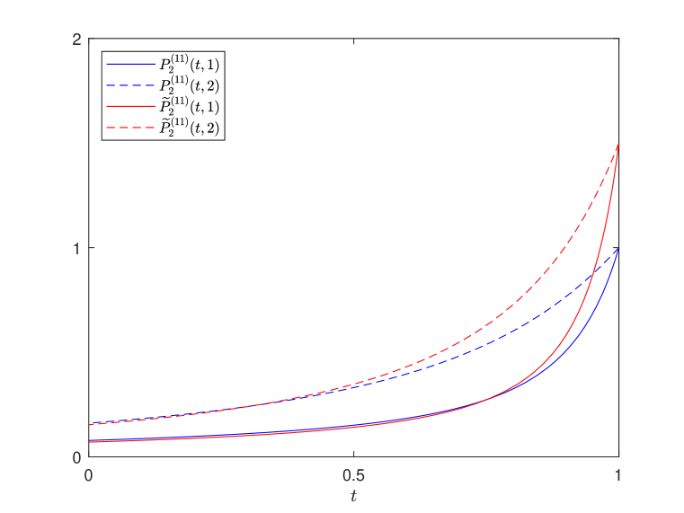
Figure 1: Riccati equations for the follower

Figure 2: Riccati equations for the leader

5 Concluding remarks

In this paper, we studied an LQ leader-follower stochastic differential game with regime switching and mean-field interactions. Conditional mean-field terms are included due to the presence of a Markov chain (just like a common noise). Some new-type Riccati equations are introduced for the first time in the literature. The open-loop Stackelberg equilibrium and its non-anticipating state feedback representation are obtained. There are several interesting problems that deserve further investigation, in particular, the existence and uniqueness results of the Riccati equations (41) and (43).

References

• [1] B. Acciaio, J. Backhoff-Veraguas, R. Carmona, Extended mean field control problems: stochastic maximum principle and transport perspective, SIAM J. Control Optim., 57 (2019), 3666–3693.
• [2] A. Bensoussan, B. Djehiche, H. Tembine, S. C. P. Yam, Mean-field-type games with jump and regime switching, Dyn. Games Appl., 10 (2020), 19–57.
• [3] R. Buckdahn, B. Djehiche, J. Li, S. Peng, Mean-field backward stochastic differential equations: A limit approach, Ann. Probab., 37 (2009), 1524–1565.
• [4] R. Buckdahn, J. Li, S. Peng, Mean-field backward stochastic differential equations and related partial differential equations, Stoch. Process. Appl., 119 (2009), 3133–3154.
• [5] R. Carmona, F. Delarue, Probabilistic analysis of mean-field games, SIAM J. Control Optim., 51 (2013), 2705–2734.
• [6] R. Carmona, F. Delarue, Mean field forward-backward stochastic differential equations, Electron. Commun. Probab., 18 (2013), no. 68, 15 pp.
• [7] R. Carmona, F. Delarue, Forward-backward stochastic differential equations and controlled McKean-Vlasov dynamics, Ann. Probab., 43 (2015), 2647–2700.
• [8] R. Carmona, F. Delarue, Probabilistic Theory of Mean Field Games with Applications I&II, Springer, Cham, 2018.
• [9] R. Carmona, F. Delarue, D. Lacker, Mean field games with common noise, Ann. Probab., 44 (2016), 3740–3803.
• [10] R. Carmona, X. Zhu, A probabilistic approach to mean field games with major and minor players, Ann. Appl. Probab., 26 (2016), 1535–1580.
• [11] J. Jian, P. Lai, Q. Song, J. Ye, LQG mean field games with a Markov chain as its common niose, arXiv: 2106.04762v2 [math.OC], 2021.
• [12] R. Josa-Fombellida, J. P. Rincón-Zapatero, Minimization of risks in pension funding by means of contributions and portfolio selection, Insurance Math. Econom., 29 (2001), 35–45.
• [13] I. Karatzas, S. E. Shreve, Broanian Motion and Stochastic Calculus, Springer, New York, 1991.
• [14] J. Huang, G. Wang, J. Xiong, A maximum principle for partial information backward stochastic control problems with applications, SIAM J. Control Optim., 48 (2009), 2106–2117.
• [15] M. Huang, P. E. Caines, R. P. Malhamé, Large-population cost-coupled LQG problems with nonuniform agents: individual-mass behavior and decentralized $\varepsilon$-Nash equilibria, IEEE Trans. Automat. Control, 52 (2007), 1560–1571.
• [16] J. Li, Stochastic maximum principle in the mean-field controls, Automatica, 48 (2012), 366–373.
• [17] N. Li, J. Xiong, Z. Yu, Linear-quadratic generalized Stackelberg games with jump-diffusion processes and related forward-backward stochastic differential equations, Science China Math., 64 (2021), 2091–2116.
• [18] T, Li, J. F. Zhang, Asymptotically optimal decentralized control for large population stochastic multiagent systems, IEEE Trans. Automat. Control, 53 (2008), 1643–1660.
• [19] X. Li, J. Sun, J. Xiong, Linear quadratic optimal control problems for mean-field backward stochastic differential equations, Appl. Math. Optim., 1 (2019), 223–250.
• [20] S. Lv, Z. Wu, Q. Zhang, The Dynkin game with regime switching and applications to pricing game options, Ann. Oper. Res., 313 (2022), 1159–1182.
• [21] S. Lv, J. Xiong, Hybrid optimal impulse control, Automatica, 140 (2022), 110233.
• [22] J. Ma, P. Protter, J. Yong, Solving forward-backward stochastic differential equations explicitly-a four-step scheme, Probab. Theory Relat. Fields, 98 (1994), 339–359.
• [23] J. Moon, Linear-quadratic stochastic Stackelberg differential games for jump-diffusion systems, SIAM J. Control Optim., 59 (2021), 954–976.
• [24] S. L. Nguyen, D. T. Nguyen, G. Yin, A stochastic maximum principle for switching diffusions using conditional mean-fields with applications to control problems, ESAIM Control Optim. Calc. Var., 26 (2020), 69.
• [25] S. L. Nguyen, G. Yin, T. A. Hoang, Laws of large numbers for systems with mean-field interactions and Markovian switching, Stoch. Process. Appl., 130 (2020), 262–296.
• [26] S. L. Nguyen, G. Yin, D. T. Nguyen, A general stochastic maximum principle for mean-field controls with regime switching, Appl. Math. Optim., 84 (2021), 3255–3294.
• [27] J. Shi, G. Wang, J. Xiong, Leader-follower stochastic differential game with asymmetric information and applications, Automatica, 63 (2016), 60–73.
• [28] Q. Song, R. H. Stockbridge, C. Zhu, On optimal harvesting problems in random environments, SIAM J. Control Optim., 49 (2011), 859–889.
• [29] G. Wang, Z. Wu, A maximum principle for mean-field stochastic control system with noisy observation, Automatica, 137 (2022), 110135.
• [30] G. Wang, C. Zhang, W. Zhang, Stochastic maximum principle for mean-field type optimal control under partial information, IEEE Trans. Automat. Control, 59 (2014), 522–528.
• [31] J. Xiong, An Introduction to Stochastic Filtering Theory, Oxford University Press, Oxford, 2008.
• [32] J. Yong, A leader-follower stochastic linear quadratic differential game, SIAM J. Control Optim., 41 (2002), 1015–1041.
• [33] J. Yong, Linear-quadratic optimal control problems for mean-field stochastic differential equations, SIAM J. Control Optim., 51 (2013), 2809–2838.
• [34] Q. Zhang, Stock trading: An optimal selling rule, SIAM J. Control Optim., 40 (2001), 64–87.
• [35] X. Zhang, X. Li, J. Xiong, Open-loop and closed-loop solvabilities for stochastic linear quadratic optimal control problems of Markovian regime switching system, ESAIM Control Optim. Calc. Var., 27 (2021), Paper No. 69, 35 pp.
• [36] X. Zhang, Z. Sun, J. Xiong, A general stochastic maximum principle for a Markov-modulated jump-diffusion model of mean-field type, SIAM J. Control Optim., 56 (2018), 2563–2592.
• [37] Y. Zheng, J. Shi, A Stackelberg game of backward stochastic differential equations with applications, Dyn. Games Appl., 10 (2020), 968–992.
• [38] X. Y. Zhou, G. Yin, Markowitz’s mean-variance portfolio selection with regime switching: A continuous-time model, SIAM J. Control Optim., 42 (2003), 1466–1482.
• [39] C. Zhu, Optimal control of the risk process in a regime-switching environment, Automatica, 47 (2011), 1570–1579.