Hamilton cycles in a semi-random graph model

Abstract.

We show that whp we can build a Hamilton cycle after at most $1.85n$ rounds in a particular semi-random model. In this model, in one round, we are given a uniform random $v\in[n]$ and then we can add an arbitrary edge $\left\{v,w\right\}$. Our result improves on $2.016n$ in [5].

1. Introduction

We consider the following semi-random graph model. We start with $G_{0}$ equal to the empty graph on vertex set $[n]$. We then obtain $G_{i+1}$ from $G_{i},i\geq 0$ as follows: we are presented with a uniform random $v\in[n]$ and then we can choose to add an arbitrary edge $\left\{v,w\right\}$ to $G_{i}$. This model was suggested by Peleg Michaeli and first explored in Ben-Eliezer, Hefetz, Kronenberg, Parczyk, Shikhelman and Stojaković [1]. Further research on the model can be found in Ben-Eliezer, Gishboliner, Hefetz and Krivelevich [2]; Gao, Kamiński, MacRury and Prałat[3]; and Gao, Macrury and Prałat[4, 5]. In particular [5] shows that whp one can construct a Hamilton cycle in this model in at most $2.016n$ rounds.

In this short note we modify the algorithm of [5] and prove:

Theorem 1.1.

In the semi-random model, there is a strategy for constructing a Hamilton cycle in at most $1.85n$ rounds.

2. Outline and Algorithm

Our algorithm and analysis are largely similar to those of [5], so let us recapitulate the broad strokes. They maintain a large and growing path, and a set of isolated nodes. When an isolated node is presented they join it to the tail of the path. When a path node $v$ is presented, they generate a “stubedge” (our name, not theirs) to a random isolated node $w$; later, if a path node $v^{\prime}$ adjacent to $v$ is presented, they generate edge $\left\{v^{\prime},w\right\}$ and use it to insert the vertex $w$ into the path between $v$ and $v^{\prime}$. These stubs are vital when the path is long and there are few isolated vertices: at that point, isolated vertices are rarely presented, while many stubs are generated. Note that by “birthday paradox” reasoning, only $\Theta(\sqrt{n})$ stubs are needed before there is a good chance of a neighboring vertex being presented.

As observed in [5], stubs can also be used to turn a Hamilton path into a Hamilton cycle in $o(n)$ rounds. Assume w.l.o.g. that the path vertices are in sequence $1,\ldots,n$. From each vertex $v$ presented, we generate a stubedge randomly to vertex $1$ or $n$. If $v$ had a stubedge to $n$ and later $v+1$ is presented, joining $v+1$ to $1$ creates a Hamilton cycle, using $1,\ldots,v$; $v+1,\ldots,n$; the stubedge $\left\{v,n\right\}$; and the new edge $\left\{v+1,1\right\}$. This takes expected time $O(1/\sqrt{n})$.

As in [5], we maintain a large and growing path and isolated nodes, but a key difference is that we also maintain a set of pairs. When an isolated node $v$ is presented, rather than joining it to the tail of the path, we join it to another isolated node $v^{\prime}$ to make a pair. When a vertex $v$ in a pair is presented, we join the pair to the tail of the path. Stubs are used to incorporate into the path either an isolated node, just as in [5], or a pair: If a stubedge goes from $v$ to a paired vertex $w$, and a path neighbor $v^{\prime}$ of $v$ is presented, joining $v^{\prime}$ to the partner $w^{\prime}$ of $w$ allows replacement of the edge $\left\{v,v^{\prime}\right\}$ with the path $v,w,w^{\prime},v^{\prime}$.

The motivation for this is simple. If an isolated vertex $v$ is presented, the number of components decreases by 1 whether $v$ is added to the path or paired with another vertex $v^{\prime}$: in this sense, equal progress is made either way. Ignoring the use of stubs, in the [5] algorithm, after $v$ is presented and joined to the path, to join $v^{\prime}$ to the path we would have to wait for $v^{\prime}$ to be presented. In the paired version, after $v$ is presented and paired with $v^{\prime}$, to join the pair of them to the path we wait until either $v$ or $v^{\prime}$ is presented; this takes half as long in expectation.

With regard to the stubs, the two versions are similar. As just noted, the number of components (isolated vertices or pairs) needing to be incorporated into the path (including by use of stubs) is the same either way. The only drawback of the paired version is that the path’s growth is somewhat delayed, so there are fewer early opportunities to create and use stubs.

3. Algorithm and Differential Equations

Our algorithm is largely the same as the main “fully randomized algorithm” of [5]. We do not employ any equivalent of their initial “degree-greedy” phase, although doing so would probably improve our results slightly. Like them, we run the main algorithm until the path is nearly but not quite complete, so that it can be analysed by the differential equation method. We finish up by appealing to the “clean-up” algorithm of [5, Lemma 2.5].

We now describe our algorithm in detail but briefly, then present the corresponding differential equations. As said, we maintain a path $P$, and non-path vertices $V$ consisting of isolated vertices $V_{1}$ and paired vertices $V_{2}$.

A stubedge goes from a path vertex we call the stubroot or simply stub to a non-path vertex we call a stubend. We say a stubroot with $i$ stubedges has stub-degree $i$; we will also call it an $i$-stubroot, and let $S_{i}$ be the set of such vertices. We limit the stub-degree to at most 3, so $S=S_{1}\cup S_{2}\cup S_{3}$ is the set of all stubroots. (There are never more than about $0.001n$ 3-stubs, and restricting the degree to at most 2 as in [5] only increases our completion time by about $0.002n$, from about $1.8465n$ to $1.8482n$.)

Each path vertex is one of four types, and when focussing on type we will use this font: a stub; a path-neighbor of a stub, called a stubneighbor; a clear vertex, which if presented will become a stub; or a blocked vertex, which is essentially useless.

In an abuse of notation, reusing the letters for the sets to denote their cardinality, let $P=P(t)$ denote the number of vertices on the path at time $t$, $V_{1}=V_{1}(t)$ the number of isolated vertices, $V_{2}=V_{2}(t)$ the number of vertices in pairs, $S_{i}=S_{i}(t)$ the number of $i$-stubs (for $i\in\left\{1,2,3\right\}$), $V(t)=V_{1}(t)+V_{2}(t)$, and $S(t)=S_{1}(t)+S_{2}(t)+S_{3}(t)$. We explore the expected changes in these quantities in one round.

Our algorithm will preserve the following property.

Property 3.1.

Within path-distance 2 of any stub there is no other stub nor any clear vertex, and the total number of clear vertices is exactly $P-5S$.

We discuss this in case (C1) below.

3.1. Description of the Algorithm

We list the actions taken after a (random) vertex is presented. The description below is valid as long as there remain at least 2 isolated vertices, and we will stop the algorithm long before that is an issue.

1. The presented vertex $v$ is clear. Choose a random non-path vertex $w$ and create a stubedge from $v$ to $w$, making $v$ a 1-stubroot. Change the type of $v$ from clear to stub, and if $v$ has path-distance 5 or more from other stubs, change the types of its path neighbors and second-neighbors, respectively, to stubneighbor and blocked, i.e., BNSNB. If $v$ is at distance 4 from the next stub to the right, make the types from $v$ to the next stub be SNBNS, and if distance 3, then SNNS.

   This changes 5 or fewer vertices from clear to another type. If fewer, then artificially change the type of additional clear vertices to blocked to make it exactly 5. This, and the fact that there is no clear nor stub vertex within path-distance 2 of $v$, preserve Property 3.1. There is no constraint on where the artificially blocked vertices should be, and they need not even stay fixed from round to round.

2. The presented vertex $v$ is a stub with $i$ stubneighbors, $i=1,2$. Choose a random non-path vertex $w$ and create a stubedge from $v$ to $w$, making $v$ an $(i+1)$-stubroot.

3. The presented vertex $v$ is a stubneighbor of a stub vertex $u$. By Property 3.1, $u$ is uniquely determined. Randomly choose one of $u$’s stubneighbors, $w$. Lengthen the path by removing the edge $\left\{v,u\right\}$, then adding the path $u,w,v$ (if $w\in V_{1}$, making the new edge $\left\{v,w\right\}$) or $u,w,w^{\prime},v$ (if $w\in V_{2}$ and $w,w^{\prime}$ is a pair, making the new edge $\left\{v,w^{\prime}\right\}$). If $u$’s degree was 2 or 3, $u$ becomes an $(i-1)$-stub.

   If $u$’s degree was 1, the stub disappears: $u$ and its two associated stubneighbor vertices become clear, as do its two associated blocked vertices unless they must remain blocked by proximity to some other stub. If necessary, change one or two other blocked vertices to clear to preserve Property 3.1.

   The stubedge $\left\{v,w\right\}$ becomes a path edge, and all other stubedges into $w$ (and $w^{\prime}$, if relevant) are deleted. This results in reducing the stub-degrees of other stubroots, and possibly their deletion.

4. The presented vertex $v$ is on the path, but blocked or a stub of degree 3. Do nothing.

5. The presented vertex $v$ is isolated. Choose another isolated vertex $v^{\prime}$ at random and make a pair $v,v^{\prime}$.

6. The presented vertex $v$ is one of a pair, with some $v^{\prime}$. Add $v,v^{\prime}$ to the tail of the path. As in (C3), delete all stubs to $v$ and $v^{\prime}$.

Lemma 3.2.

In (C6), each stubedge has probability $2/V(t)$ that its stubend is either $v$ or $v^{\prime}$, and these events are independent. In (C3) where $w$ was isolated, each stubedge except $\left\{v,w\right\}$ has probability $1/V(t)$ that its stubend is $w$, and these events are independent. In (C3) where $w$ was paired with $w^{\prime}$, each stubedge except $\left\{v,w\right\}$ has probability $2/V(t)$ that its stubend is either $w$ or $w^{\prime}$, and these events are independent.

This is analogous to a claim within [5, Lemma 2.2]. For (C6) the Lemma is immediate as the stubs to $v$ and $v^{\prime}$ are independent of their getting paired or joining the path. In the (C3) cases, though, there is a potential issue of size-biased sampling that is not explicitly addressed in the proof in [5], and so we give a proof sketch. The issue is that $w$ being the stubend of the chosen stubedge biases $w$ to have higher stub-degree (e.g., $w$ could not have been selected if it had no stub edges), suggesting that other stubedges are also more likely to have $w$ as stubend.

Proof.

Imagine that, when created, the stubedges are not revealed. They remain, then, uniformly random between the stubroots (whose stub-degrees are “known”) and non-path vertices. Only when the stubroot $v$ is determined and one of its stubedges is chosen, reveal (or, indeed, generate) the stubedge: this determines $w$. Only then, reveal (or generate) the other stubedges: each is equally likely to lead to $w$ or any other non-path vertex (including $w^{\prime}$, if relevant). So that we can apply the argument again in later rounds, we can reveal just the stubedges incident to $w$ (and $w^{\prime}$ if relevant): after deleting them, the other stubedges remain unrevealed and uniformly random. ∎

Alternatively, one may argue from the perspective that if one sample is taken from a population of i.i.d. Poisson $\lambda$ random variables, in proportion to the variables’ values, the sampled value $X$ is not Poisson $\lambda$ (for example, it cannot be 0), but $X-1$ is Poisson $\lambda$.

3.2. Derivation of the Equations

The following equations are valid as long as $P(t)\leq(1-\epsilon)n$ where $\epsilon>0$ is arbitrarily small; anyway the differential equation method can only be applied through such time. The error terms below are sometimes naturally $O(1/n)$ and sometimes $O(1/V(t))$, but with this assumption we always write them as $O(1/n)$.

3.2.1. ${\bf P(t)}$

$$\mathbb{E}(P(t+1)\mid G_{t})=P(t)+\frac{2V_{2}(t)}{n}+\frac{2S(t)}{n}\cdot\frac{V_{1}(t)+2V_{2}(t)}{V(t)}+O(1/n).$$ (1)

(C6):

$V_{2}(t)/n$ is the probability that a paired vertex is presented. The path length increases by 2.

(C3):

$2S(t)/n$ is the probability that a stubneighbor is presented. By Property 3.1 the stubroot $v$ is uniquely determined, and one of its stubedges $\left\{v,w\right\}$ is chosen randomly. With probability $V_{1}(t)/V(t)$, $w$ is isolated and the path length increases by 1; with probability $V_{2}(t)/V(t)$, $w$ is paired and the path length increases by 2.

3.2.2. ${\bf V_{1}(t)}$

$$\mathbb{E}(V_{1}(t+1)\mid G_{t})=V_{1}(t)-\frac{2V_{1}(t)}{n}-\frac{2S(t)}{n}\cdot\frac{V_{1}(t)}{V(t)}+O(1/n).$$ (2)

(C5):

$V_{1}(t)/n$ is the probability that an isolated vertex is presented. The vertex is paired with another isolated vertex and the number of isolated vertices decreases by 2.

(C3):

$2S(t)/n$ is the probability that a stubneighbor is presented. As in section 3.2.1’s (C3), the chosen stubend of the stub is isolated with probability $V_{1}(t)/V(t)$ and the number of isolated vertices decreases by 1.

3.2.3. ${\bf V_{2}(t)}$

$$\mathbb{E}(V_{2}(t+1)\mid G_{t})=V_{2}(t)-\frac{2V_{2}(t)}{n}+\frac{2V_{1}(t)}{n}-\frac{2S(t)}{n}\cdot\frac{2V_{2}(t)}{V(t)}+O(1/n).$$ (3)

(C6):

$V_{2}(t)/n$ is the probability that a paired vertex is presented. The path is extended using this pair, and the number of paired vertices decreases by 2.

(C5):

$V_{1}(t)/n$ is the probability that an isolated vertex is presented. The vertex is paired with another isolated vertex and the number of paired vertices increases by 2.

(C3):

$2S(t)/n$ is the probability that a stubneighbor is presented. The chosen stubend of the stub is paired with probability $V_{2}(t)/V(t)$, and the number of paired vertices decreases by 2.

At this point the reader will observe that the expected change in $n=P(t)+V_{1}(t)+V_{2}(t)$ is zero, as it should be.

3.2.4. ${\bf S_{1}(t)}$

$$\mathbb{E}(S_{1}(t+1)\mid G_{t}) =S_{1}(t)+\frac{P(t)-5S(t)}{n}-\frac{S_{1}(t)}{n}-\frac{2S_{1}(t)}{n}+\frac{2S_{2}(t)}{n}$$

$$\hskip 10.00002pt+\frac{2S(t)}{n}\cdot\frac{V_{1}(t)+2V_{2}(t)}{V(t)^{2}}\cdot(2S_{2}(t)-S_{1}(t))$$

$$\hskip 10.00002pt+\frac{V_{2}(t)}{n}\cdot\frac{2}{V(t)}\cdot(2S_{2}(t)-S_{1}(t))+O(1/n).$$ (4)

(C1):

$(P(t)-5S(t))/n$ is the probability that a clear vertex is presented. It becomes a 1-stub and $S_{1}(t)$ increases by 1.

(C2, $i=1$):

$S_{1}(t)/n$ is the probability that a 1-stub of the path is presented. It becomes a 2-stub, and $S_{1}(t)$ decreases by 1.

(C3, $i=1$):

$2S_{1}(t)/n$ is the probability that a neighbor of a 1-stub is presented. The stub is used and $S_{1}(t)$ decreases by 1.

(C3, $i=2$):

$2S_{2}(t)/n$ is the probability that a neighbor of a 2-stub is presented. The stub is used and $S_{1}(t)$ increases by 1.

(C3):

$2S(t)/n$ is the probability that a stubneighbor is presented. As in previous cases, the stub $v$ is determined and one of its stubedges $\left\{v,w\right\}$ is chosen randomly. Edge $\left\{v,w\right\}$ becomes a path edge, and is no longer a stubedge; this is captured by the previous two cases.

All other stubedges into $w$, and its pair-partner $w^{\prime}$ if any, are deleted. With probability $V_{1}(t)/V(t)$, $w$ was isolated, in which case by Lemma 3.2 each stubedge has probability $1/V(t)$ of having $w$ as stubend. With probability $V_{2}(t)/V(t)$, $w$ was paired with some $w^{\prime}$, in which case by Lemma 3.2 each stubend has probability $2/V(t)$ of having $w$ or $w^{\prime}$ as stubend. This gives the probability in the next term.

The effect in that term is that each $S_{2}$ vertex has 2 stubedges whose potential deletion turns it into an $S_{1}$ vertex, increasing $S_{1}$ by 1, while each $S_{1}$ vertex has 1 stubedge whose potential deletion turns it into a clear vertex, decreasing $S_{1}$ by 1.

(C6):

$V_{2}(t)/n$ is the probability that a paired vertex is presented. As in the preceding case, by Lemma 3.2 each stubedge has probability $2/V(t)$ of having either element of the pair as stubend and thus being deleted. The effect is that of the previous case.

3.2.5. $\bf S_{2}(t)$

$$\mathbb{E}(S_{2}(t+1)\mid G_{t}) =S_{2}(t)+\frac{S_{1}(t)}{n}-\frac{S_{2}(t)}{n}-\frac{2S_{2}(t)}{n}+\frac{2S_{3}(t)}{n}$$

$$\hskip 10.00002pt+\left[\frac{2S(t)}{n}\cdot\frac{V_{1}(t)+2V_{2}(t)}{V(t)^{2}}+\frac{V_{2}(t)}{n}\cdot\frac{2}{V(t)}\right]\cdot(3S_{3}(t)-2S_{2}(t))+O(1/n).$$ (5)

(C2, $i=1$):

$S_{1}(t)/n$ is the probability that a 1-stubroot of the path is presented. It becomes a 2-stubroot, and $S_{2}(t)$ increases by 1.

(C2, $i=2$):

$S_{2}(t)/n$ is the probability that a 2-stubroot of the path is presented. It becomes a 3-stubroot, and $S_{2}(t)$ decreases by 1.

(C3, $i=2$):

$2S_{2}(t)/n$ is the probability that a neighbor of a 2-stubroot is presented. The stub is used and $S_{2}(t)$ decreases by 1.

(C3, $i=3$):

$2S_{3}(t)/n$ is the probability that a neighbor of a 3-stubroot is presented. The stub is used and $S_{2}(t)$ increases by 1.

(C3),(C6):

Analogous to (C3) and (C6) of section 3.2.4, here combined.

3.2.6. $\bf S_{3}(t)$

$$\mathbb{E}(S_{3}(t+1)\mid G_{t}) =S_{3}(t)+\frac{S_{2}(t)}{n}-\frac{2S_{3}(t)}{n}$$

$$\hskip 10.00002pt-\left[\frac{2S(t)}{n}\cdot\frac{V_{1}(t)+2V_{2}(t)}{V(t)^{2}}+\frac{V_{2}(t)}{n}\cdot\frac{2}{V(t)}\right]\cdot 3S_{3}(t)+O(1/n).$$ (6)

(C2, $i=2$):

$S_{2}(t)/n$ is the probability that a 2-stub vertex of the path is presented. It becomes a 2-stub, and $S_{3}(t)$ increases by 1.

(C3, $i=3$):

$2S_{3}(t)/n$ is the probability that a neighbor of a 3-stub is presented. The stub is used and $S_{3}(t)$ decreases by 1.

(C3),(C6):

Analogous to the corresponding case of section 3.2.5.

The equations (1) – (3.2.6) lead to the following differential equations in the usual way: we let $\tau=t/n$ and $p(\tau)=P(t)/n,v_{1}(\tau)=V_{1}(t)/n$ etc. The initial conditions are $v_{1}(0)=1,p(0)=v_{2}(0)=\cdots=s_{3}(0)=0$.

$$\begin{split}p^{\prime}&=2v_{2}+\frac{2s(v_{1}+2v_{2})}{v}.\\ v_{1}^{\prime}&=-2v_{1}-\frac{2sv_{1}}{v}.\\ v_{2}^{\prime}&=-2v_{2}+2v_{1}-\frac{4sv_{2}}{v}.\\ s_{1}^{\prime}&=p-5s-3s_{1}+2s_{2}+\left[\frac{2s(v_{1}+2v_{2})}{v^{2}}+\frac{2v_{2}(t)}{v}\right](2s_{2}-s_{1}).\\ s_{2}^{\prime}&=s_{1}-3s_{2}+2s_{3}+\left[\frac{2s(v_{1}+2v_{2})}{v^{2}}+\frac{2v_{2}}{v}\right](3s_{3}-2s_{2}).\\ s_{3}^{\prime}&=s_{2}-2s_{3}-\left[\frac{2s(v_{1}+2v_{2})}{v^{2}}+\frac{2v_{2}}{v}\right](3s_{3}).\\ \end{split}$$ (7)

A numerical simulation of the differential equations is shown in Figure 1. It shows that $v_{1}(\tau^{*})+v_{2}(\tau^{*})\approx 0$ and $p(\tau^{*})\approx 1$ for $\tau^{*}\approx 1.85$. Justification of the use of the differential equation method follows as in [5]. As in [5], we use the differential equation method to analyse the algorithm until the path has length $(1-\epsilon)n$, for some suitably small $\epsilon$. After this we apply the clean-up algorithm of [5, Lemma 2.5] to construct a Hamilton cycle in a further $O(\sqrt{\epsilon}n+n^{3/4}\log^{2}n)$ rounds.

4. Concluding Remarks

Our combining of isolated vertices into pairs leads to a substantial speedup of the algorithm compared with [5], despite our skipping their first, “degree greedy” phase. We allowed for stub degrees up to 3 where [5] goes up only to 2, but, observing that the number of degree-3 stubs is never more than about $0.001n$, this seems to have been unimportant. Further improvements could probably be made.

First, since pairs gave a big gain, it is natural to consider paths of 3 vertices (“triplets”) or more. We have not tried it, but it appears that this cannot help. Specifically, if an isolated vertex $v$ is presented, there would appear to be no advantage in using $v$ to extend a “pair” $Q$ to a 3-vertex path, over concatenating $v$ to the main path. Either way, the number of components is the same. Either way, $Q$ must eventually be brought into $P$, either when one of its endpoints is presented (no difference in whether $p$ is added to $Q$ or not, as either way $Q$ has two endpoints), or when a stubedge to one of $Q$’s endpoints is used (again, with no advantage to $v$ over $Q$’s earlier endpoint).

Other improvements, possibly challenging to analyse, would come from choices intuitively more sensible than the uniformly random choices made by our algorithm.

One such is to restore the “degree greedy” approach from [5] that we discarded: when generating stubedges, let each go to a (random) non-path vertex of lowest stub-degree.

Another, when generating stubedges, is to favour paired vertices over isolated ones. We have some weak evidence that generating stubedges only to non-paired vertices up to some time, then uniformly to all non-paired vertices, is better than generating them uniformly throughout.

Another strategy is, in the case where a 2- or 3-stub is used, to select a stubedge to a non-path vertex of low stub degree, and/or to favor an isolated vertex over a paired one (or vice versa).

Returning to the idea of using “triples” as well as pairs, potentially, small advantages could be found if, for example, we linked $v$ with $Q$ only if $v$ were the stubend of more stubedges than the $Q$-endpoint it extends.

It would be very satisfying in its own right to better understand the natural stub process, where a presented vertex becomes a new stubroot unless it is already a stubroot or stubneighbor, i.e., if it is at path distance at least 2 from every existing stub. This in contradistinction to the easier-to-analyse process taken from [5] and described in (C1), where a presented vertex becomes a stub only if it is at path distance at least 3 from every existing stub, and not blocked. In the natural process, the number of stubneighbors will be between 1 and 2 times the number of stubroots (not 2 times, as used in (C3)) but it is not clear how to find the typical number, nor give a good lower bound. Presumably more stubroots will be produced, but it is not clear how to control the likelihood that a presented vertex will become a stub; indeed, nothing about the process is clear.

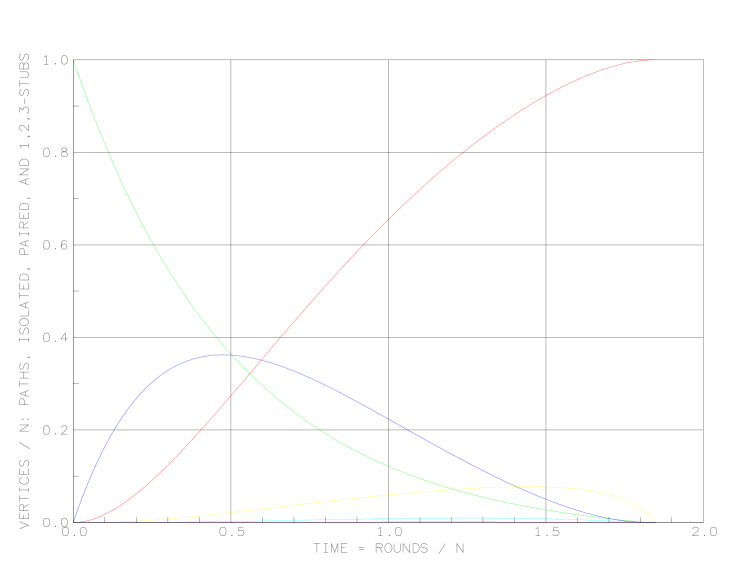
Figure 1. The differential equations simulated, as a function of time (rounds divided by $n$). Path length $P$ (as a multiple of $n$) is shown in red, isolated vertices $V_{1}$ in green, paired vertices $V_{2}$ in blue, and degree 1-, 2-, and 3-stubs $S_{i}$ in yellow, turquoise, and magenta. (The figure is clearer in some PDF viewers than others.)

References

- [1] O. Ben-Eliezer, D. Hefetz, G. Kronenberg, O. Parczyk, C. Shikhelman, M. Stojaković (2020). Semi‐random graph process. Random Structures & Algorithms, 56, 648–675.
- [2] O. Ben-Eliezer, L. Gishboliner, D. Hefetz, M. Krivelevich. Very fast construction of bounded-degree spanning graphs via the semi-random graph process. Random Structures & Algorithms, 57(4), 892–919.
- [3] P. Gao, B. Kamiński, C. MacRury, and P. Prałat. 2022. Hamilton cycles in the semi-random graph process. Eur. J. Comb. 99, C (Jan 2022).
- [4] P. Gao, C. MacRury, and P. Prałat. Perfect Matchings in the Semirandom Graph Process. SIAM J. Discrete Mathematics 36(2) (2022).
- [5] P. Gao, C. MacRury, and P. Prałat. A Fully Adaptive Strategy for Hamiltonian Cycles in the Semi-Random Graph Process. 2022. arXiv, https://arxiv.org/abs/2205.02350.