The Schwarzian octahedron recurrence (dSKP equation) II: geometric systems

Abstract

We consider nine geometric systems: Miquel dynamics, P-nets, integrable cross-ratio maps, discrete holomorphic functions, orthogonal circle patterns, polygon recutting, circle intersection dynamics, (corrugated) pentagram maps and the short diagonal hyperplane map. Using a unified framework, for each system we prove an explicit expression for the solution as a function of the initial data; more precisely, we show that the solution is equal to the ratio of two partition functions of an oriented dimer model on an Aztec diamond whose face weights are constructed from the initial data. Then, we study the Devron property [Gli15], which states the following: if the system starts from initial data that is singular for the backwards dynamics, this singularity is expected to reoccur after a finite number of steps of the forwards dynamics. Again, using a unified framework, we prove this Devron property for all of the above geometric systems, for different kinds of singular initial data. In doing so, we obtain new singularity results and also known ones [Gli15, Yao14]. Our general method consists in proving that these nine geometric systems are all related to the Schwarzian octahedron recurrence (dSKP equation), and then to rely on the companion paper [AdTM22], where we study this recurrence in general, prove explicit expressions and singularity results.

1 Introduction

The dSKP equation is a relation on six variables that arises as a discretization of the Schwarzian Kadomtsev-Petviashvili hierarchy [BK98a, BK98b], hence its name. In this paper, this relation is embedded in the octahedral-tetrahedral lattice $\mathcal{L}$ defined by:

$$\mathcal{L}=\left\{p=(i,j,k)\in\mathbb{Z}^{3}:i+j+k\in 2\mathbb{Z}\right\}.$$

Consider a function $x:\mathcal{L}\to\hat{\mathbb{C}}$. We say that $x$ satisfies the dSKP recurrence, or Schwarzian octahedron recurrence, if

$$\frac{(x_{-e_{3}}-x_{e_{2}})(x_{-e_{1}}-x_{e_{3}})(x_{-e_{2}}-x_{e_{1}})}{(x_{e_{2}}-x_{-e_{1}})(x_{e_{3}}-x_{-e_{2}})(x_{e_{1}}-x_{-e_{3}})}=-1,$$ (1.1)

where $(e_{1},e_{2},e_{3})$ is the canonical basis of $\mathbb{Z}^{3}$, $x_{q}(p):=x(p+q)$ for every $q\in(e_{i})_{i=1}^{3}$, and the relation is evaluated at any $p\in\mathbb{Z}^{3}\setminus\mathcal{L}$. The target space $\hat{\mathbb{C}}$ is an affine chart of ${\mathbb{C}\mathrm{P}}^{1}$.

Suppose that we are given initial data $\left(a_{i,j}\right)_{i,j\in\mathbb{Z}^{2}}$. One starts with values $x(i,j,[i+j]_{2})=a_{i,j}$, where $[n]_{p}\in\{0,\dots,p-1\}$ denotes the value of $n$ modulo $p$, and apply the dSKP recurrence to get any value $x(i,j,k)$ with $(i,j,k)\in\mathcal{L}$ and $k>[i+j]_{2}$. The solution is a rational function in the initial data $a$. One of the main contributions of the companion paper [AdTM22] is an explicit combinatorial expression of this rational function as the ratio of two partition functions of an associated oriented dimer model. Other main contributions consist in the study of singular initial conditions. These results, specified to the cases needed in the current paper, are recalled in Section 2.

The purpose of this paper is to use the general framework of the first paper to study discrete geometric systems. The systems considered here come in three groups. The first group consists solely of Miquel dynamics (Section 3), it is the only example we consider that has two-dimensional initial data. The second group consists of integrable cross-ratio maps (Section 5) and special cases thereof, which are discrete holomorphic functions (Section 6), polygon recutting (Section 7) and circle intersection dynamics (Section 8). As a special case of discrete holomorphic functions we also consider orthogonal circle patterns (Section 6.5), also known as Schramm circle packings. The third group consists of the corrugated pentagram map for $N$-corrugated polygons (Section 9.4), which for $N=2$ is simply called the pentagram map (Section 9) as well as the short diagonal hyperplane map (Section 10). A special role is played by P-nets (Section 4), which arise both as a restriction of discrete holomorphic functions but also correspond to the case of $N=1$ of the corrugated pentagram map.

For each system, we prove an explicit expression for the solution as a function of the initial data. Finding the explicit solution to any one of these systems is a result in its own right. Thus it is all the more practical that we can obtain all solutions to all the systems we present here from one underlying result. Let us mention that in the special case of Schramm’s circle packings some specific solutions were studied, see for example [AB00] and references therein. As an example, let us state our result for discrete holomorphic functions, see also Corollary 6.4 for a precise statement.

Theorem 1.1.

Let $z:\mathbb{Z}^{2}\rightarrow\hat{\mathbb{C}}$ be a discrete holomorphic function, and consider the graph $\mathbb{Z}^{2}$ with face weights $(a_{i,j})_{(i,j)\in\mathbb{Z}^{2}}$ given by,

$$a_{i,j}=\begin{cases}z_{\frac{i+j+[i+j]_{2}}{2},\frac{-(i+j)+[i+j]_{2}}{2}}&\text{ if }[i-j]_{4}\in\{0,3\},\\ z_{\frac{i+j+[i+j]_{2}}{2},\frac{-(i+j)+[i+j]_{2}}{2}+1}&\text{ if }[i-j]_{4}\in\{1,2\}.\end{cases}$$

Then, for all $(i,j)\in\mathbb{Z}^{2}$ such that $i+j\geq 2$, we have

$$z_{i,j} =\begin{cases}Y(A_{i+j-2}[z_{i^{\prime},(j-1)^{\prime}}],a)&\text{ if $[i+j]_{4}\in\{0,3\}$},\\ Y(A_{i+j-2}[z_{i^{\prime},(j-1)^{\prime}+1}],a)&\text{ if $[i+j]_{4}\in\{1,2\}$,}\end{cases}$$

where generically $A_{k}[a_{i,j}]$ denotes the Aztec diamond of size $k$ centered at a face with weight $a_{i,j}$; $Y(A_{k}[a_{i,j}],a)$ is the corresponding ratio function of oriented dimers, and for all $i,j\in\mathbb{Z}$, $(i^{\prime},j^{\prime}):=\bigl{(}\frac{i-j+[i-j]_{2}}{2},\frac{-(i-j)+[i-j]_{2}}{2}\bigr{)}.$

The proofs of these “explicit expression theorems” all follow the same pattern. They rely on a key lemma relating the geometric system to the dSKP equation. Then, they consist in applying our general explicit expression dSKP result [AdTM22, Theorem 1.1], written in the context of this paper as Theorem 2.2 below.

We next turn to proving singularity results for geometric systems, whose meaning we now explain. Let us assume that $T$ is an operator describing the dynamics, whether it is the iteration of the dSKP equation in general or the dynamics of some geometric system. For some choices of initial data, referred to as singular, $T^{-1}$ is not defined, however proceeding forwards with the dynamics seems possible to some extent. Integrable systems are believed to have a common property, known as the Devron property [Gli15], that can be thought of as a variant of the more common singularity confinement property initially introduced in relation with integrability of discrete equations [GRP91, HV98]. The Devron property says the following: if some periodic initial data is singular for the backwards dynamics, it should become singular after a finite number of steps of the fowards dynamics. In the companion paper, we identify initial data, that we call $(m,p)$-Devron initial data, and prove that the dSKP recurrence features the Devron property [AdTM22, Theorem 1.6]. We also obtain stronger results for a particularly symmetric case of $(m,1)$-Devron data referred to as $m$-Dodgson initial data [AdTM22, Corollary 1.5]. For general dSKP, our singularity results are new. However, in several geometric systems that we consider, singularity results have already been obtained by Glick [Gli15] and Yao [Yao14]. What we provide in this paper is a unified framework, relying on the Devron property of general dSKP, which allows us to identify the number of iterations after which a singular initial data reoccurs and, in some cases, compute the position of the returning singularity. Table 1 summarizes the results of this paper, those that are known and the new ones.

System	Initial condition	Steps	Reference	Citations
Miquel dynamics	$m$-Dodgson	$m-1$	Theorem 3.7	new
P-nets	$m$-Dodgson	$m-1$	Theorem 4.4	[Gli15, Yao14]
P-nets	$m$-Dodgson*	$m-2$	Theorem 4.5	new
Int. cr-maps	$(m,2)$-Devron	$2m-2$	Theorem 5.7	new
D. hol. f., $[m]_{2}=1$	$(m,2)$-Devron	$2m-2$	Theorem 6.10	[Yao14]
D. hol. f., $[m]_{2}=0$	$(m,2)$-Devron	$2m-3$	Theorem 6.10	new
D. hol. f., $[m]_{2}=0$	$(m,2)$-Devron*	$2m-4$	Theorem 6.11	new
Orthogonal CP	$(2m,2)$-Devron	$m-2$	Corollary 6.17	new
Polygon recutting	$(m,1)$-Devron	$m-1$	Theorem 7.7	[Gli15]
Circle intersection dyn.	$(m,1)$-Devron	$m-1$	Theorem 8.4	new
Circle intersection dyn.	$(m,2)$-Devron	$2m-4$	Theorem 8.5	new
Pentagram map	$m$-Dodgson	$m-1$	Theorem 9.5	[Gli15, Yao14]
Pentagram map	$(m,2)$-Devron	$2m-4$	Theorem 9.6	new
$N$-corrugated pent. map	$m$-Dodgson	$2m-2$	Theorem 9.12	[Gli15, Yao14]
Short diagonal hyp. map	$(m,2)$-Devron	$m-2$	Theorem 10.4	new

Table 1: An overview of the singularity results presented in this paper and the literature. A * denotes some additional algebraic constraint on the initial conditions.

As an example, let us state one of our (new) results for discrete holomorphic functions, see also Theorem 6.11.

Theorem 1.2.

Let $m\in 2\mathbb{N}+2$, and let $\tilde{z}$ be an $m$-periodic discrete holomorphic function such that $\tilde{z}_{i,0}=0$ for all $i\in 2\mathbb{Z}$, and such that

$$\sum_{i=0}^{m-1}\frac{(-1)^{i}}{\tilde{z}_{2i+1,1}}=0.$$ (1.2)

Assume that we can apply the propagation map $T$ to $(\tilde{z}_{0},\tilde{z}_{1})$ at least $2m-4$ times. Then, for all $i\in 2\mathbb{Z}+1$,

$$\tilde{z}_{i,2m-3}=\left(\frac{1}{m}\sum_{\ell=0}^{m-1}\frac{1}{\tilde{z}_{2\ell+1,1}}\right)^{-1}.$$ (1.3)

In other words, $\tilde{z}_{2m-3}$ is constant with value equal to the harmonic mean of $\tilde{z}_{1}$.

As mentioned above, our proofs of these results follow as corollaries of our dSKP singularity results [AdTM22]. The latter are recalled in the context of this paper in Section 2.2. The techniques used to obtain the dSKP results are of a combinatorial nature, and computing the position of a singularity amounts to finding eigenvectors of associated matrices. In comparison, Glick [Gli15] uses various methods to prove the Devron property, including “rescaled” variations of Dodgson condensation for the dKP equation and a similar method for Y-systems, which he then applies to the pentagram maps and its generalizations. He also uses multi-dimensional consistency in the case of polygon recutting. On the other side, Yao [Yao14] uses lifts to high-dimensional spaces and careful analysis of certain subspaces and invariants to prove the Devron property and the position of the recurring singularity.

Let us note that our singularity theorems provide upper bounds for the number of iterations of the respective dynamics. We have done extensive numerical verifications, so we are confident that generically within the respective assumptions, the upper bounds are actually tight. A proof of this would require to provide example solutions in each case. In principle, as we provide explicit formulas for all the dynamics, our methods also provide the algebraic conditions on the initial conditions, such that the dynamics terminate before the upper bound is reached. Apart from the two premature singularity reoccurrences mentioned above, we have not investigated these cases any further.

As a conclusion to this introduction, let us turn to open questions. First, we believe that hexagonal circle patterns with constant intersection angles [AB03, BH03] fall into our framework as well, but we have not investigated them in detail. Moreover, on the one hand, there has not been much research devoted yet to the study of the Devron property, on the other hand, it is easy to verify numerically that it appears in many geometric systems. This naturally leads to a lot of open questions. For example, we propose Conjecture 7.8 on the position of the recurring singularity in polygon recutting. Moreover, Conjecture 9.8 proposes a new type of recurring singularity, that does not seem to be a special case of a $(m,p)$-Devron singularity. Answering this conjecture would most likely help to also prove Conjecture 9.7, on the geometric nature of the $(m,2)$-Devron singularity in the pentagram map case. We believe these conjectures are well within the power of the general dSKP framework we developed.

There are also some geometric systems that feature the Devron property, for which it is not clear whether they are describable via the dSKP equation. In particular, we mention a higher dimensional version of discrete holomorphic functions in Remark 6.12. There are also three conjectures in [Gli15, Section 9]. The first we prove in Theorem 8.5. The second concerns a generalization of the pentagram map introduced by Khesin and Soloviev [KS13]; we prove it in Theorem 10.4, using results of Glick and Pylyavskyy [GP16] in combination with our framework. The last conjecture mentioned by Glick on the so called Schubert flip is open, and it is not clear whether there is a relation to the dSKP equation.

Finally, there is an intriguing coincidence of the evaluation of two Aztec diamonds of different sizes and with different weights. Both describe the propagation of discrete holomorphic functions, once via P-nets and once via integrable cross-ratio maps, see Question 6.7.

Outline of the paper

In Section 2 we recall the prerequisites from the companion paper [AdTM22]. Then, the following sections are dedicated to the different geometric systems. Section 3: Miquel dynamics, Section 4: P-nets, Section 5: integrable cross ratio maps, Section 6: discrete holomorphic functions and orthogonal circle patterns, Section 7: polygon recutting, Section 8: circle intersection dynamics, Section 9: $N$-corrugated polygons and pentagram map, Section 10: short diagonal hyperplane map. All geometric systems sections essentially follow the same structure which consists of: describing the geometric system, establishing the key lemma relating it to the dSKP equation, proving the explicit expression result, and then showing singularity results.

Acknowledgments

The first author would like to thank Max Glick and Sanjay Ramassamy for helpful discussions. He is supported by the Deutsche Forschungsgemeinschaft (DFG) Collaborative Research Center TRR 109 “Discretization in Geometry and Dynamics” as well as the by the MHI and Foundation of the ENS through the ENS-MHI Chair in Mathematics. The second and third authors are partially supported by the DIMERS project ANR-18-CE40-0033 funded by the French National Research Agency. The authors would also like to thank Claude-Michel Viallet for interesting discussions on singularity confinements.

2 Prerequisites

In this section we recall the results of the first paper [AdTM22], in special cases that appear in geometric systems.

The dSKP recurrence lives on vertices of the octahedral-tetrahedral lattice $\mathcal{L}$ defined as:

$$\mathcal{L}=\left\{p=(i,j,k)\in\mathbb{Z}^{3}:i+j+k\in 2\mathbb{Z}\right\}.$$

Definition 2.1.

A function $x:\mathcal{L}\rightarrow\hat{\mathbb{C}}$ satisfies the dSKP recurrence, if

$$\frac{(x_{-e_{3}}-x_{e_{2}})(x_{-e_{1}}-x_{e_{3}})(x_{-e_{2}}-x_{e_{1}})}{(x_{e_{2}}-x_{-e_{1}})(x_{e_{3}}-x_{-e_{2}})(x_{e_{1}}-x_{-e_{3}})}=-1,$$ (2.1)

holds evaluated at every point $p$ of $\mathbb{Z}^{3}\setminus\mathcal{L}$, where $x_{q}(p):=x(q+p)$ for every $q\in(\pm e_{i})_{i=1}^{3}$. More generally, if $A\subset\mathcal{L}$ and $x:A\to\hat{\mathbb{C}}$, we say that $x$ satisfies the dSKP recurrence on $A$ when (2.1) holds whenever all the points are in $A$.

The target space $\hat{\mathbb{C}}$ of the dSKP recurrence is an affine chart of the complex projective line ${\mathbb{C}\mathrm{P}}^{1}$, defined as follows. Consider the equivalence relation $\sim$ on $\mathbb{C}^{2}$ such that for $v,v^{\prime}\in\mathbb{C}^{2}$ we have $v\sim v^{\prime}$ if there is a $\lambda\in\mathbb{C}\setminus\{0\}$ such that $v=\lambda v^{\prime}$. Every point in the projective line is an equivalence class $[v]=\{v^{\prime}:v^{\prime}\sim v\}$ for some $v\in\mathbb{C}^{2}\setminus\{(0,0)\}$, that is

$${\mathbb{C}\mathrm{P}}^{1}=\{[v]:v\in\mathbb{C}^{2}\setminus\{(0,0)\}\}=\left(\mathbb{C}^{2}\setminus\{(0,0)\}\right)/\sim.$$

Then $\hat{\mathbb{C}}=\mathbb{C}\cup\{\infty\}$ is an affine chart of ${\mathbb{C}\mathrm{P}}^{1}$: every point $z\in\mathbb{C}\subset\hat{\mathbb{C}}$ corresponds to $[z,1]$ in ${\mathbb{C}\mathrm{P}}^{1}$ and $\infty\in\hat{\mathbb{C}}$ corresponds to $[1,0]$. In the affine chart one can perform the usual arithmetic operations on ${\mathbb{C}\mathrm{P}}^{1}$. One can even apply the naive calculation rules $z+\infty=\infty,z/\infty=0$ etc., see [RG11, Section 17]. Note that solutions to the dSKP equation are invariant under projective transformations, and the iteration of dSKP has a natural interpretation in terms of a projective involution, see [AdTM22, Remark 2.3].

Given $(a_{i,j})_{(i,j)\in\mathbb{Z}^{2}}$, define the initial condition

$$\forall\ (i,j)\in\mathbb{Z}^{2},\quad x(i,j,[i+j]_{2})=a_{i,j},$$ (2.2)

where $[n]_{p}$ generically denotes the value of $n$ modulo $p$, taken in $\{0,\dots,p-1\}$. The idea is that if $x$ satisfies the dSKP recurrence on $\mathcal{L}$, its values are determined by the initial conditions $\left(a_{i,j}\right)_{(i,j)\in\mathbb{Z}^{2}}$. Giving a combinatorial expression for this function of the initial conditions is the point of the next paragraph.

Note that in the following sections we assume that all initial data for dSKP are generic, in the sense that the data propagates to the whole lattice $\mathcal{L}$. When we study singularities, we assume that the data is as generic as possible under the assumption of the initial singularity. We will not repeat these assumptions in the following.

2.1 Explicit solution

Consider the square lattice, with faces indexed by $\mathbb{Z}^{2}$. The face indexed by $(i,j)$ is equipped with the weight $a_{i,j}$. For $k\geq 0$, define the Aztec diamond of size $k$ centered at $a_{i,j}$, denoted by $A_{k}(i,j)$ or $A_{k}[a_{i,j}]$, to be the subgraph centered at $(i,j)$ whose internal faces are those with labels $(i^{\prime},j^{\prime})$ such that $|i^{\prime}-i|+|j^{\prime}-j|<k$, see Figure 1. We call open faces those with label $(i^{\prime},j^{\prime})$ such that $|i^{\prime}-i|+|j^{\prime}-j|=k$, and denote by $F$ the set of internal and open faces of $A_{k}[a_{i,j}]$.

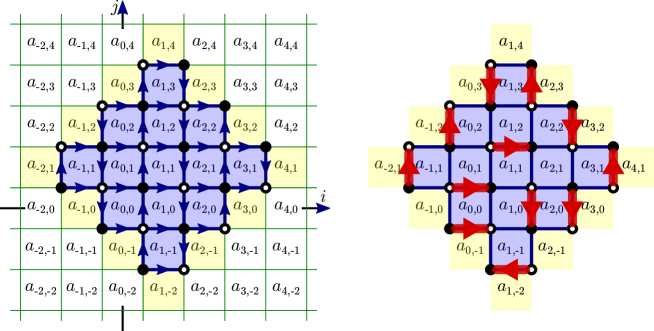
Figure 1: Left: the Aztec diamond of size $3$, $A_{3}[a_{1,1}]$, in blue, shown as a bipartite graph with a Kasteleyn orientation, with its internal faces in blue, and its open faces in yellow. Right: an example of an oriented dimer configuration on this graph. The ratio of partition functions is equal to $x(1,1,4)$.

As $A_{k}[a_{i,j}]$ is bipartite, we can decompose its vertex set $V$ into black and white vertices: $V=B\sqcup W$. In general, for a finite, planar bipartite graph $G$, let $\vec{E}$ be the set of its directed edges. A Kasteleyn orientation [Kas61] is, in our case, a skew-symmetric function $\varphi$ from $\vec{E}$ to $\{-1,1\}$ such that, for every internal face $f$ of degree $2k$ we have

$$\prod_{wb\in\partial f}\varphi_{(w,b)}=(-1)^{k+1}.$$

This corresponds to an orientation of edges of the graph: an edge $e=wb$ is oriented from $w$ to $b$ when $\varphi_{(w,b)}=1$, and from $b$ to $w$ when $\varphi_{(w,b)}=-1$. By Kasteleyn [Kas67], such an orientation of $G$ exists; in our case, an example is displayed in Figure 1.

An oriented dimer configuration of $A_{k}[a_{i,j}]$ is a subset of oriented edges $\vec{\mathsf{M}}$ such that its undirected version $\mathsf{M}$ is a dimer configuration - that is, it touches every vertex exactly once. Denote by $\vec{\mathscr{M}}$ the set of oriented dimer configurations of $A_{k}[a_{i,j}]$.

Given a Kasteleyn orientation $\varphi$, and an oriented edge $\vec{e}$, denote by $f(\vec{e})$ the (internal or open) face to the right of $\vec{e}$. The weight of an oriented dimer configurations $\vec{\mathsf{M}}$ is

$$w(\vec{\mathsf{M}})=\prod_{\vec{e}\in\vec{\mathsf{M}}}\varphi_{\vec{e}}\ a_{f(\vec{e})},$$ (2.3)

and the corresponding partition function is

$$Z(A_{k}[a_{i,j}],a,\varphi)=\sum_{\vec{\mathsf{M}}\in\vec{\mathscr{M}}}w(\vec{\mathsf{M}}).$$

We consider the weighted ratio of partition functions, defined by

$$Y(A_{k}[a_{i,j}],a)=\biggl{(}\,\prod_{f\in F}a_{f}\biggr{)}\ \frac{Z(A_{k}[a_{i,j}],a^{-1},\varphi)}{Z(A_{k}[a_{i,j}],a,\varphi)}.$$

It is also referred to as the ratio function of oriented dimers. Note that the partition function in the numerator uses the inverse face weights $a^{-1}_{i,j}$ to define the weight of configurations (2.3). The ratio of partition function does not depend on the choice of $\varphi$, see [AdTM22, Proposition 3.2]. This definition can be extended consistently to Aztec diamonds of size $0$ by setting $Y(A_{0}[a_{i,j}],a)=a_{i,j}$.

The following is a special case of [AdTM22, Theorem 3.4], detailed in [AdTM22, Example 3.5].

Theorem 2.2 ([AdTM22]).

If $x:\mathcal{L}\rightarrow\hat{\mathbb{C}}$ satisfies the dSKP recurrence with initial condition (2.2), then for every $(i,j,k)\in\mathcal{L}$ such that $k\geq 1$,

$$x(i,j,k)=Y(A_{k-1}[a_{i,j}],a).$$

In [AdTM22], we also prove an algebraic expression for the solution of the dSKP recurrence. To state it, it is easier to rotate the previous Aztec diamond by $45$ degrees, as in Figure 2. Recall that $B$ denotes the set of black vertices of this Aztec diamond, and that $F$ denotes the set of (internal or open) faces. Each face $f\in F$ corresponds to a weight, simply denoted by $a_{f}$. We define a linear operator $D$ going from $\mathbb{C}^{B}\oplus\mathbb{C}^{B}$ to $\mathbb{C}^{F}$, whose entries are the following: if $b$ is in the first copy of $B$ and $f\in F$ is adjacent to $b$, $D_{f,b}=\pm 1$, with $+1$ if $b$ is on the right or above $f$ and $-1$ otherwise. If $b^{\prime}$ is in the second copy of $B$ and $f\in F$ is adjacent to $b^{\prime}$, $D_{f,b^{\prime}}=\pm a_{f}$, with the same sign rule as before, see Figure 2. All the other entries are zero.

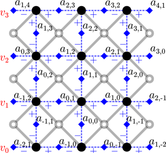
Figure 2: The same data as Figure 1 rotated by 45 degrees; again $(i,j,k)=(1,1,4)$. The elements of $B$ are shown as black dots, and those of $F$ are shown as blue diamonds. The nonzero entries of the operator $D$ correspond to the blue dashed lines, and their sign is indicated. The red labels are entries of the vector $v\in\mathbb{C}^{F}$ in the statement of Theorem 2.3.

Note that $2|B|=|F|-1$, so $D^{T}$ always has a nontrivial kernel. We can now express the dSKP solution, using [AdTM22, Theorem 5.3] after a change of index convention.

Theorem 2.3 ([AdTM22]).

Let $x:\mathcal{L}\rightarrow\hat{\mathbb{C}}$ satisfy the dSKP recurrence with initial condition (2.2). Let $(i,j,k)\in\mathcal{L}$ such that $k\geq 1$, and $D$ be the operator defined from $(A_{k-1}[a_{i,j}],a)$. Let $v\in\mathbb{C}^{F}$ be a nonzero vector such that

$$D^{T}\ v=0.$$ (2.4)

Denote by $v_{0},\dots,v_{k-1}$ the entries of $v$ corresponding to the $k$ leftmost elements of $F$, with respective face weights $a_{i-k+1,j},\dots,a_{i,j+k-1}$. Then, the ratio function of oriented dimers can be expressed as:

$$Y(A_{k-1}[a_{i,j}],a)=\frac{\sum_{\ell=0}^{k-1}a_{i-k+\ell+1,j+\ell}\,v_{\ell}}{\sum_{\ell=0}^{k-1}v_{\ell}}.$$

As argued in the proof of [AdTM22, Theorem 5.3], this statement should be understood as an equality of expression in formal variables $(a_{i,j})$; the entries $(v_{\ell})$ are themselves rational functions of the $(a_{i,j})$. One might wonder if this equality holds when $\dim\ker D^{T}\geq 2$. The following proposition, combined with the fact that there exists global solutions to the dSKP recurrence (see [AdTM22, Example 2.4]) implies that this is generically not the case: if one sees $D^{T}$ as a formal matrix in the $(a_{i,j})$ variables, then its kernel is always one-dimensional.

Proposition 2.4.

With the same notation as in Theorem 2.3, suppose that the initial conditions $(a_{i,j})$ are such that $\dim\ker D^{T}\geq 2$. Then $Y(A_{k-1}[a_{i,j}],a)$ is undefined in $\hat{\mathbb{C}}$, and so is $x(i,j,k)$.

Proof.

Suppose that there are two free vectors in $\ker D^{T}$. By a linear combination, there is a nonzero vector $v\in\ker D^{T}$ such that $\sum_{\ell=0}^{k-1}v_{\ell}=0$, so by Theorem 2.3, $Y(A_{k-1}[a_{i,j}],a)$ has to be $\infty$ or undefined (if at the same time $\sum_{\ell=0}^{k-1}a_{i-k+\ell,j+\ell}\,v_{\ell}=0$). Similarly, we can get another nonzero vector $v^{\prime}\in\ker D^{T}$ such that $\sum_{\ell=0}^{k-1}a_{i-k+\ell,j+\ell}\,v^{\prime}_{\ell}=0$, so that $Y(A_{k-1}[a_{i,j}],a)$ has to be $0$ or undefined (if at the same time $\sum_{\ell=0}^{k-1}v^{\prime}_{\ell}=0$). Since Theorem 2.3 holds for any choice of non-zero vector in $\ker D^{T}$, the only solution that satisfies both conditions is that it is undefined. Using Theorem 2.2, $x(i,j,k)$ is undefined as well. ∎

2.2 Singularities

We now recall the results of [AdTM22] about singular initial conditions. Note that we return to the unrotated version of the Aztec diamond as in Figure 1.

In some special cases, we prove a simpler expression for the solution $x(i,j,k)$ than the one given by Theorem 2.3. This is the case when $a_{i,j}=d$ whenever $(i,j)\in\mathbb{Z}^{2}$ and $[i+j]_{2}=0$, and $d$ is a constant. Then $x(i,j,k)$ can be expressed in terms of the inverse of a matrix $N$, of size $k\times k$, whose coefficients are the shifted inverses of the non-zero initial conditions that enter into the computation of $x(i,j,k)$. The following is taken from [AdTM22, Corollary 5.10].

Proposition 2.5 ([AdTM22]).

Suppose that for all $(i,j)\in\mathbb{Z}^{2}$ such that $[i+j]_{2}=0$, $a_{i,j}=d$. Let $(i,j,k)\in\mathcal{L}$ with $k\geq 1$. Consider the matrix $N=\left(N_{i^{\prime},j^{\prime}}\right)_{0\leq i^{\prime},j^{\prime}\leq k-1}$ with entries

$$N_{i^{\prime},j^{\prime}}=\frac{1}{a_{i-i^{\prime}+j^{\prime},j+k-1-i^{\prime}-j^{\prime}}-d}.$$

Then

$$x(i,j,k)=d+\sum_{0\leq i^{\prime},j^{\prime}\leq k-1}N^{-1}_{i^{\prime},j^{\prime}},$$

where the sum is over entries of the inverse matrix $N^{-1}$.

For example, if $d=0$, in the case of Figure 1 (that is $(i,j,k)=(1,1,4)$), this matrix is

$$N=\begin{pmatrix}a_{1,4}^{-1}&a_{2,3}^{-1}&a_{3,2}^{-1}&a_{4,1}^{-1}\\ a_{0,3}^{-1}&a_{1,2}^{-1}&a_{2,1}^{-1}&a_{3,0}^{-1}\\ a_{-1,2}^{-1}&a_{0,1}^{-1}&a_{1,0}^{-1}&a_{2,-1}^{-1}\\ a_{-2,1}^{-1}&a_{-1,0}^{-1}&a_{0,-1}^{-1}&a_{1,-2}^{-1}\end{pmatrix}.$$

We now turn to initial conditions with periodicity. For $m\geq 1$, we say that the initial conditions are $m$-doubly periodic if $a_{i,j}=a_{i+m,j+m}=a_{i+m,j-m}$. We say that they are $m$-Dodgson initial conditions if they are $m$-doubly periodic and in addition, for all $(i,j)\in\mathbb{Z}^{2}$ with $[i+j]_{2}=0$, $a_{i,j}=d$ where $d$ is a constant. Then, as a corollary to Proposition 2.5, we prove that at height $m$ (that is, after $m-1$ iterations of the dSKP recurrence), the same kind of special conditions reappear. This implies that the values of $x$ at height $m+1$ are not defined. The following is part of [AdTM22, Theorem 1.4].

Corollary 2.6 ([AdTM22]).

For $m$-Dodgson initial conditions, for every $(i,j)\in\mathbb{Z}^{2}$ such that $(i,j,m)\in\mathcal{L}$, $x(i,j,m)$ is independent of $i,j$.

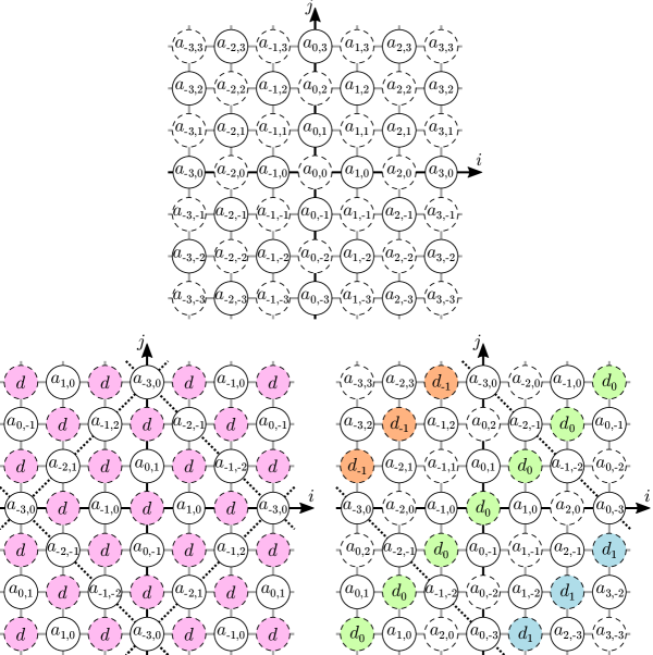
Figure 3: Initial data $(a_{i,j})$ for the dSKP recurrence. Variables in dashed circles lie at height $k=0$, while those in solid circles lie at height $k=1$. Top: generic. Bottom left: $3$-Dodgson; an elementary pattern is shown as a dashed square, and particular values at height $0$ are shown in purple. Bottom right: $(3,2)$-Devron; constant diagonals are shown in orange, green, blue.

In some cases it is possible to give a simple expression for this constant value on the layer at height $m$. More precisely, we prove such an expression when the NW-SE diagonals at height $1$ contain data that are cyclic permutations of each other. This corresponds to [AdTM22, Corollary 1.5].

Corollary 2.7 ([AdTM22]).

Suppose that the initial conditions are $m$-Dodgson, and suppose in addition that $d=0$ and that for some $p\not\in m\mathbb{Z}$, when $[i+j]_{2}=1$, $a_{i,j}=a_{i+p+1,j-p+1}$. Then, for all $(i,j)\in\mathbb{Z}^{2}$ such that $(i,j,m)\in\mathcal{L}$, $x(i,j,m)$ is the harmonic mean of the $m$ different values of the initial data:

$$x(i,j,m)=\left(\frac{1}{m}\sum_{i=0}^{m-1}a_{i,1-i}^{-1}\right)^{-1}.$$

Another, more general case of singularity is the following. We say that the initial data is $m$-simply periodic when for all $i,j$, $a_{i,j}=a_{i+m,j+m}$. For $m,p\geq 1$, we say that they are $(m,p)$-Devron initial conditions if they are $m$-simply periodic and in addition, for all $i,j$ with $[i-j]_{2p}=0$, $a_{i,j}=a_{i+1,j+1}$. This amounts to having every $p$-th SW-NE diagonal at height $0$ constant, see Figure 3, bottom right. We show in [AdTM22, Theorem 1.6] that this kind of special conditions reappears at height $(m-2)p+2$ (that is, after $(m-2)p+1$ applications of the dSKP recurrence):

Theorem 2.8 ([AdTM22]).

For $(m,p)$-Devron initial data, let $k=(m-2)p+2$. Then, for all $(i,j)\in\mathbb{Z}^{2}$ such that $[i-j-mp]_{2p}=0$, we have

$$x(i,j,k)=x(i+1,j+1,k).$$

3 Miquel dynamics

3.1 Circle patterns and Miquel dynamics

Any line or circle in the Euclidean sense in $\mathbb{C}\subset\hat{\mathbb{C}}$ is considered to be a (generalized) circle in ${\mathbb{C}\mathrm{P}}^{1}$. It is straightforward to verify that this definition of circles is invariant under projective transformations, as defined in [AdTM22, Remark 2.3]. Möbius transformations are all transformations that are compositions of projective transformations and complex conjugations $z\mapsto\bar{z}$. Clearly, the definition of circles above is also more generally invariant under all Möbius transformations. In an affine chart $\hat{\mathbb{C}}$ the center of a circle in the Euclidean sense is the Euclidean center and the center of a Euclidean line is $\infty$. Circle centers are not a projective or Möbius invariant notion but they are still useful in a fixed affine chart.

Definition 3.1.

A (square grid) circle pattern is a map $p:\mathbb{Z}^{2}\rightarrow\hat{\mathbb{C}}$, such that for all $(i,j)\in\mathbb{Z}^{2}$, there is a circle $c_{i,j}$ such that $p_{i,j},p_{i+1,j},p_{i+1,j+1},p_{i,j+1}\in c_{i,j}$. Denote by $t_{i,j}$ the center of the circle $c_{i,j}$, by $c:\mathbb{Z}^{2}\rightarrow\{\text{Circles of ${\mathbb{C}\mathrm{P}}^{1}$}\}$, the map corresponding to circles, and by $t:\mathbb{Z}^{2}\rightarrow\mathbb{C}$ the one corresponding to circle centers.

In the generic case, having both the circles $c_{i,j}$ and the intersection points $p_{i,j}$ is pointless, as the circles define the intersection points and vice versa. However we will look at non-generic cases later, so it is handy to have both descriptions ready. Note that we will use the terminology circle pattern both for the map $p$ and for the map $c$.

Definition 3.2.

A (square grid) t-realization is a map $t:\mathbb{Z}^{2}\rightarrow\mathbb{C}$, such that, for all $(i,j)\in\mathbb{Z}^{2}$,

$$\frac{(t_{i+1,j}-t_{i,j})(t_{i-1,j}-t_{i,j})}{(t_{i,j+1}-t_{i,j})(t_{i,j-1}-t_{i,j})}\in\mathbb{R}.$$ (3.1)

We use the term t-realization rather than t-embedding [CLR20] since in Definition 3.2 we do not ask the full requirements of a t-embedding, i.e., we do not ask that it corresponds to an embedded graph with convex faces. Note that t-embeddings have also previously appeared under the name of Coulomb gauge in [KLRR18]. The term t-realization has been used as a relaxation of t-embedding before [CLR21, Section 4.1], although we relax even more as we do not require the quantity in Definition 3.2 to be real positive. In the discrete differential geometry community, t-realizations are the planar case of conical nets, which are also studied separately [Mü15].

The circle centers of a circle pattern are a t-realization [Aff21, KLRR18]. A t-realization does not uniquely define a circle pattern, but it does so up to the choice of one of the intersection points.

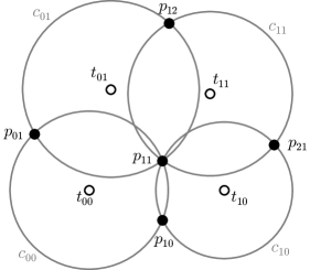
Figure 4: Left: Labeling in a circle pattern. Right: The six circles of a Miquel configuration.

In a square grid circle pattern, every circle has exactly four neighbouring circles, see Figure 4. These four circles intersect in eight points, four of which belong to the original circle. Miquel’s six circles theorem [Miq38] states that the four other points belong to a sixth circle. Following [Ram18], we can now introduce Miquel dynamics. The parity of a circle $c_{i,j}$ is defined to be the parity of $i+j$.

Definition 3.3.

Miquel dynamics is the dynamics $T$ mapping circle patterns to circle patterns such that, for every $k\geq 1$, $T^{k}(c)$ is $T^{k-1}(c)$, except that if $k$ is even (resp. odd) every odd (even) circle is replaced with the sixth circle that exists due to Miquel’s theorem; $T^{k}(t)$ denotes the corresponding dynamics on circle centers.

A relation of Miquel dynamics to dSKP is given by the next lemma.

Lemma 3.4 ([KLRR18, Aff21]).

Let $t$ be a t-realization associated to a circle pattern $c$. Then, for all $(i,j)\in\mathbb{Z}^{2}$ such that $[i+j]_{2}=0$, we have

$$\frac{(t_{i,j}-t_{i+1,j})(t_{i,j+1}-T(t)_{i,j})(t_{i-1,j}-t_{i,j-1})}{(t_{i+1,j}-t_{i,j+1})(T(t)_{i,j}-t_{i-1,j})(t_{i,j-1}-t_{i,j})}=-1.$$ (3.2)

A consequence of Lemma 3.4 is that $T(t)$ only depends on the circle centers $t$ and needs no additional information on the actual circle pattern $c$.

3.2 Explicit solution

Using Theorem 2.2, we provide an explicit expression for $T^{k}(t)$ using the ratio function of oriented dimers of the Aztec diamond. Recall from Section 2.1 that for the square lattice $\mathbb{Z}^{2}$ with face weights $(a_{i,j})_{(i,j)\in\mathbb{Z}^{2}}$, $A_{k}[a_{i,j}]$ denotes the Aztec diamond of size $k$ centered at $a_{i,j}$.

Theorem 3.5.

Let $t:\mathbb{Z}^{2}\rightarrow\mathbb{C}$ be a t-realization, and consider the graph $\mathbb{Z}^{2}$ with face-weights $(a_{i,j})_{(i,j)\in\mathbb{Z}^{2}}$ given by

$$a_{i,j}=t_{i,j}.$$

Then, for all $(i,j)\in\mathbb{Z}^{2},\,k\geq 1$ such that $[i+j+k]_{2}=1$, we have

$$T^{k}(t)_{i,j}=Y(A_{k}[t_{i,j}],t).$$

Proof.

Consider the function $x:\mathcal{L}\to\hat{\mathbb{C}}$ given by, for every $(i,j,k)$ such that $i+j+k\in 2\mathbb{Z}$, $k\geq 0$,

$$x(i,j,k)=\begin{cases}T^{k-1}(t)_{i,j}&\mbox{for }k>1,\\ t_{i,j}&\mbox{for }k\in\{0,1\}.\end{cases}$$ (3.3)

As a consequence of Lemma 3.4 we have that, for $k\geq 1$, the function $x$ satisfies the dSKP recurrence. Moreover, for all $(i,j)\in\mathbb{Z}^{2}$, the function $x$ satisfies the initial condition

$$a_{i,j}:=x(i,j,h(i,j))=x(i,j,[i+j]_{2})=t_{i,j},$$

giving the face weights of the statement.

As a consequence of Theorem 2.2, we know that $x(i,j,k)=Y(A_{k-1}[t_{i,j}],t)$. Using that $T^{k}(t)_{i,j}=x(i,j,k+1)$ ends the proof. ∎

3.3 Singularities

Using Corollary 2.6, we now study singularities of Miquel dynamics; this discussion is illustrated in Figure 5. The idea is to perform Miquel dynamics starting from a singular circle pattern (referred to as a Dodgson circle pattern) and prove that, if the singular circle pattern is moreover periodic, a similar singular circle pattern appears after a determined number of steps. This is the content of Theorem 3.7 below.

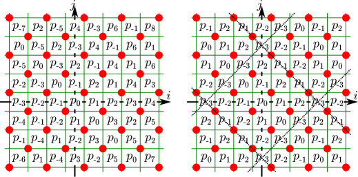
Figure 5: Left: a piece of an even Dodgson circle pattern. Every red dot corresponds to the same circle $\mathscr{D}$. Every face corresponds to a point $p^{0}_{i}$ on $\mathscr{D}$, abbreviated $p_{i}$ to alleviate the picture. Right: a doubly $m$-periodic case for $m=3$; an elementary pattern corresponds to a dotted square and repeats on the whole graph; the initial data consists in $2m=6$ points $p_{-3},p_{-2},p_{-1},p_{0},p_{1},p_{2}$ on $\mathscr{D}$, and $m^{2}=9$ circles distinct from $\mathscr{D}$, each passing through two points $p_{i},p_{j}$ with $i\not\equiv j\mod 2$. A geometric realisation is shown in Figure 6, where the green circle can be thought of as $\mathscr{D}$ and its six vertices as $p_{-3},\dots,p_{2}$ in cyclic order.

Definition 3.6.

Let $\mathscr{D}\subset\mathbb{C}$ be a fixed circle and let $p^{0}:\mathbb{Z}\rightarrow\mathscr{D}$. An even Dodgson circle pattern (with respect to $\mathscr{D}$) is a circle pattern $p^{\mathscr{D}}:\mathbb{Z}^{2}\rightarrow\mathbb{C}$ such that, for all $(i,j)\in\mathbb{Z}^{2}$,

$$p^{\mathscr{D}}_{i,j}=\begin{cases}p^{0}_{i-j}&\mbox{if }i+j\in 2\mathbb{Z}+1,\\ p^{0}_{i+j}&\mbox{if }i+j\in 2\mathbb{Z}.\end{cases}$$ (3.4)

An odd Dodgson circle pattern is defined similarly exchanging the parity in (3.4).

Note that in a circle pattern, diagonally opposite circles intersect and, in the definition of an even Dodgson circle pattern $p^{\mathscr{D}}$, even circles share three points of $\mathscr{D}$. This implies that all even circles coincide with $\mathscr{D}$, and thus all the even circle centers coincide as well. Similarly, in an odd Dodgson circle pattern, all odd circles, resp. odd circle centers, coincide. Moreover, note that the intersection points $p^{0}$ of a Dodgson circle pattern do not completely determine the circle pattern. Thus in this case it is practical to consider a circle pattern to be defined by the combination of intersection points $p$ and circles $c$.

Thus from the perspective of dSKP we are in Dodgson initial conditions, explaining the above terminology.

Let $m\geq 1$. We call a circle pattern doubly $m$-periodic if, for all $(i,j)\in\mathbb{Z}^{2}$,

$$c_{i+m,j+m}=c_{i,j}=c_{i+m,j-m}.$$

Theorem 3.7.

Let $m\geq 1$, and let $p^{\mathscr{D}}$ be a doubly $m$-periodic even Dodgson circle pattern with respect to a circle $\mathscr{D}$. Assume we can apply Miquel dynamics on $p^{\mathscr{D}}$ at least $m-1$ times. Then there is a circle $\mathscr{D}^{\prime}$ such that, when $m$ is even, resp. odd, $T^{m-1}(p^{\mathscr{D}})$ is an even, resp. odd, Dodgson circle pattern with respect to $\mathscr{D}^{\prime}$.

Proof.

By Theorem 3.5, we know that for $k\geq 1$, and all $(i,j)\in\mathbb{Z}^{2}$ such that $[i+j+k]_{2}=1$, $T^{k}(t)_{i,j}$ can be expressed as the ratio function of oriented dimers. The initial condition in the claim corresponds to those of Corollary 2.6, telling us that the singularity appears after $m-1$ steps, that is that $T^{m-1}(t)_{i,j}$ is independent of $(i,j)$ for all $(i,j)\in\mathbb{Z}^{2}$, such that $[i+j+m]_{2}=0$. This means that after $m-1$ iterations, when $m$ is even, resp. odd, all the even, resp. odd, circle centers coincide. ∎

The case of $m=2$ is just Miquel’s theorem. The case of $m=3$ has some additional symmetries compared to general $m>3$, see Figure 6. For $m=3$ all circles and intersection points occurring in Miquel dynamics yield a configuration that consists of 20 circles and 30 intersection points. On every circle there are six intersection points and through every intersection point passes 4 circles.

Other singularities like column-wise and single-column coincidences of circles in the initial-data exist as well. The same arguments as in the Dodgson Miquel case apply, but there is nothing of particular additional interest to be said. Thus we conclude the discussion of Miquel dynamics here.

Figure 6: Miquel Dodgson for $m=3$ yields an incidence theorem involving 20 circles. Green + blue is an even Dodgson circle pattern, and red + purple an odd Dodgson circle pattern, and the second pair is obtained from the first by two applications of Miquel dynamics.

4 P-nets

4.1 Definitions

We now consider P-nets, which were introduced in the study of discrete isothermic nets [BP99, Section 6.2] and relations of these surfaces to discrete integrable systems. P-nets are also related to discrete quadratic holomorphic differentials by Lam [Lam16]. Although more abstract, P-nets have a geometric realisation in terms of discrete holomorphic functions, see Section 6.3, and occur in orthogonal circle patterns, see Section 6.5.

Definition 4.1.

A P-net is a map $p:\mathbb{Z}^{2}\rightarrow\hat{\mathbb{C}}$ such that, for all $(i,j)\in\mathbb{Z}^{2}$,

$$\frac{1}{p_{i+1,j}-p_{i,j}}-\frac{1}{p_{i,j+1}-p_{i,j}}+\frac{1}{p_{i-1,j}-p_{i,j}}-\frac{1}{p_{i,j-1}-p_{i,j}}=0.$$ (4.1)

In fact, this definition is equivalent to requiring that for all $(i,j)\in\mathbb{Z}^{2}$, in any affine chart of ${\mathbb{C}\mathrm{P}}^{1}$ such that $p_{i,j}$ is at infinity, the quad $(p_{i+1,j},p_{i,j+1},p_{i-1,j},p_{i,j-1})$ is a parallelogram. This property justifies the P in P-net.

P-nets are exactly those maps from $\mathbb{Z}^{2}$ to $\hat{\mathbb{C}}$ that satisfy the following identity, see also [KS02, Section 5.2]. As we will see in the next section, this relation underlies the occurrence of the dSKP recurrence in P-nets.

Lemma 4.2.

A map $p:\mathbb{Z}^{2}\rightarrow\hat{\mathbb{C}}$ is a P-net if and only if, for all $(i,j)\in\mathbb{Z}^{2}$,

$$\frac{(p_{i,j}-p_{i+1,j})(p_{i,j+1}-p_{i,j})(p_{i-1,j}-p_{i,j-1})}{(p_{i+1,j}-p_{i,j+1})(p_{i,j}-p_{i-1,j})(p_{i,j-1}-p_{i,j})}=-1.$$ (4.2)

4.2 Explicit solution

Let $p_{j}:=(p_{i,j})_{i\in\mathbb{Z}}$ denote the points of the $j$-th row. The recurrence (4.2) of Lemma 4.2 implies that the points $p_{j+1}$ are determined by the points $p_{j}$ and $p_{j-1}$. Therefore we view two rows of data as initial data, and this determines the whole P-net.

Note that this framework is different from Miquel dynamics, where we viewed the whole circle pattern as initial data.

The next theorem makes this more explicit and proves that, for all $i\in\mathbb{Z},j\geq 1$, the point $p_{i,j}$ is equal to the ratio function of oriented dimers of an Aztec diamond subgraph of $\mathbb{Z}^{2}$ with face weights a subset of $(p_{i,0})_{i\in\mathbb{Z}},(p_{i,1})_{i\in\mathbb{Z}}$, see Figure 7.

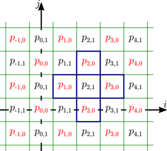
Figure 7: Face weights for the explicit solution of P-nets in Theorem 4.3 (left). The sample blue Aztec diamond is $A_{2}[p_{2,1}]$ and corresponds to the computation of $p_{2,3}$. Variables in red are those of $p_{0}$ and are all set to $0$ in Theorems 4.4 and 4.5.

Theorem 4.3.

Let $p:\mathbb{Z}^{2}\rightarrow\hat{\mathbb{C}}$ be a P-net, and consider the graph $\mathbb{Z}^{2}$ with face-weights $(a_{i,j})_{(i,j)\in\mathbb{Z}^{2}}$ given by

$$a_{i,j}=p_{i,[i+j]_{2}}.$$

Then, for all $i\in\mathbb{Z},j\geq 1$, we have

$$p_{i,j}=Y({A_{j-1}\kern-1.00006pt\left[p_{i,[j]_{2}}\right]},a).$$

Proof.

Consider the function $x:\mathcal{L}\rightarrow\hat{\mathbb{C}}$ given by

$$x(i,j,k)=p_{i,k}.$$

As a consequence of Lemma 4.2, we have that, for $k\geq 1$, the function $x$ satisfies the dSKP recurrence. Note that, for all $(i,j)\in\mathbb{Z}^{2}$, the function $x$ satisfies the initial condition

$$a_{i,j}=x(i,j,[i+j]_{2})=p_{i,[i+j]_{2}},$$

giving the face weights of the statement. As a consequence of Theorem 2.2, we know that $x(i,j,k)=Y(A_{k-1}[a_{i,j}],a)$. This implies that

$$x(i,i+j,j)=p_{i,j},\text{ and }\ a_{i,i+j}=p_{i,[2i+j]_{2}}=p_{i,[j]_{2}}.$$

The proof is concluded by using that the weighted graph $\mathbb{Z}^{2}$ is invariant by vertical translations of length 2.∎

4.3 Singularities

Assume we only know the restrictions $p_{0},p_{1}:\mathbb{Z}\rightarrow\hat{\mathbb{C}}$ of a P-net $p$ to two consecutive rows $p_{0},p_{1}$. Then, recall that by iterating Lemma 4.2, all of $p$ is uniquely reconstructable from $p_{0},p_{1}$.

Let us denote the propagation of data in a P-net as the map

$$T:(\hat{\mathbb{C}})^{\mathbb{Z}_{2}\times\mathbb{Z}}\rightarrow(\hat{\mathbb{C}})^{\mathbb{Z}_{2}\times\mathbb{Z}},\quad(p_{j},p_{j+1})\mapsto(p_{j+1},p_{j+2}).$$

Let $m\geq 1$. A P-net $p$ is said to be $m$-periodic if $p_{i,j}=p_{i+m,j}$ for all $i,j\in\mathbb{Z}$. We now study the occurrence of singularities when we start from a singular $m$-periodic P-net, i.e., an $m$-periodic P-net such that $p_{0}\equiv 0$, see also Figure 8. The recurrence of the singularity has already been proven by Glick [Gli15, Theorem 6.15], and the precise position by Yao [Yao14, Theorem 4.1]. Note that Glick and Yao call the propagation of P-nets the lower pentagram map, as it bears some resemblance to the pentagram map algebraically. We are able to obtain the result as an immediate Corollary of our general singularity theorems.

Theorem 4.4.

Let $m\geq 1$, and let $p$ be an $m$-periodic P-net such that $p_{0}\equiv 0$. Assume we can apply the propagation map $T$ to $(p_{0},p_{1})$ at least $m-1$ times. Then, for all $i\in\mathbb{Z}$, we have

$$p_{i,m}=\Bigl{(}\frac{1}{m}\sum_{\ell=0}^{m-1}p_{\ell,1}^{-1}\Bigr{)}^{-1},$$ (4.3)

that is the singularity repeats after $m-1$ steps and its value is the harmonic mean of $p_{1}$.

Proof.

By Theorem 4.3 we know that $p_{j}$ for $j\geq 1$ can be expressed via a solution of the dSKP recurrence. The initial conditions in the claim are $m$-Dodgson and also satisfy $a_{i,j}=a_{i,j+2}$, so they satisfy the hypothesis of Corollary 2.7. Therefore, the values of the dSKP solution at height $m$ (which are also the values of $p_{m}$) are all equal to the harmonic mean of $p_{1}$. ∎

Figure 8: P-net singularities. The black dot is at $0$ and corresponds to $p_{0}$; the brown dots are the values of $p_{1}$. Those are $m$-periodic with $m=3$ (left), resp. $m=4$ (center), resp. $m=5$ (right). Note that $p_{m}$ is constant.

Theorem 4.5.

Let $m\in 2\mathbb{N}+2$, and let $p$ be an $m$-periodic P-net such that $p_{0}\equiv 0$, and such that

$$\sum_{\ell=0}^{m-1}(-1)^{\ell}p_{\ell,1}^{-1}=0.$$ (4.4)

Assume we can apply the propagation map $T$ to $(p_{0},p_{1})$ at least $m-2$ times. Then, for all for all $i\in\mathbb{Z}$, we have

$$p_{i,m-1}=\Bigl{(}\frac{1}{m}\sum_{\ell=0}^{m-1}p_{\ell,1}^{-1}\Bigr{)}^{-1},$$ (4.5)

that is the singularity repeats after $m-2$ steps and its value is the harmonic mean of $p_{1}$.

Proof.

By Theorem 4.3 we know that $p_{j}$ for $j>1$ can be expressed via a solution of the dSKP recurrence. The initial conditions in the claim satisfy the hypothesis of Proposition 2.5 with $d=0$, as all initial data at height $0$ are equal to $0$ (see also Figure 7). Therefore, the value of $p_{i,m-1}$ is given by

$$p_{i,m-1}=\sum_{0\leq i^{\prime},j^{\prime}\leq m-2}N^{-1}_{i^{\prime},j^{\prime}}$$

where $N$ is the matrix of size $m-1$:

$$N=\begin{pmatrix}p^{-1}_{i,1}&p^{-1}_{i+1,1}&p^{-1}_{i+2,1}&\dots&p^{-1}_{i+m-2,1}\\ p^{-1}_{i-1,1}&p^{-1}_{i,1}&p^{-1}_{i+1,1}&\dots&p^{-1}_{i+m-3,1}\\ \vdots&&&&\vdots\\ p^{-1}_{i-m+2,1}&\dots&&&p^{-1}_{i,1}\end{pmatrix},$$

with indices taken modulo $m$. Since we suppose

$$p^{-1}_{0}+p^{-1}_{2}+\dots+p^{-1}_{m-2}=p^{-1}_{1}+p^{-1}_{3}+\dots+p^{-1}_{m-1}=:\lambda,$$

we see that $N$ applied to the vector $(1,0,1,0,\dots,1)^{T}$ gives the constant vector $\lambda(1,1,\dots,1)^{T}$. Therefore,

$$(1,0,1,0,\dots,1)^{T}=\lambda N^{-1}(1,1,\dots,1)^{T},$$

and then

$$p_{i,m-1} =\sum_{0\leq i^{\prime},j^{\prime}\leq m-2}N^{-1}_{i^{\prime},j^{\prime}}=(1,1,\dots,1)N^{-1}(1,1,\dots,1)^{T}$$

$$=\lambda^{-1}(1,1,\dots,1)(1,0,1,0,\dots,1)^{T}=\frac{m}{2}\lambda^{-1}=\Bigl{(}\frac{2}{m}\lambda\Bigr{)}^{-1}$$

$$=\Bigl{(}\frac{1}{m}\sum_{\ell=0}^{m-1}p_{\ell,1}^{-1}\Bigr{)}^{-1}.\hskip 227.62204pt\qed$$

5 Integrable cross-ratio maps and Bäcklund pairs

Integrable cross-ratio maps were introduced in relation to the discrete KdV equation [NC95, Section 2] and discrete isothermic surfaces [BP96, Section 4]. They are solutions to one of the discrete integrable equations on quad-graphs [ABS03, (Q1) with $\delta=0$]. They are also of interest because they contain many other examples as special cases, in particular the discrete holomorphic functions (see Section 6), orthogonal circle packings (see Section 6.5), polygon recutting (see Section 7) and circle intersection dynamics (see Section 8).

5.1 Definitions and properties

Definition 5.1 ([NC95, BP96]).

Let $\alpha,\beta:\mathbb{Z}\rightarrow\mathbb{C}\setminus\{0\}$ be edge-parameters. An integrable cross-ratio map is a map $z:\mathbb{Z}^{2}\rightarrow\hat{\mathbb{C}}$ such that, for all $(i,j)\in\mathbb{Z}^{2}$,

$$\operatorname{cr}(z_{i,j},z_{i+1,j},z_{i+1,j+1},z_{i,j+1}):=\frac{(z_{i,j}-z_{i+1,j})(z_{i+1,j+1}-z_{i,j+1})}{(z_{i+1,j}-z_{i+1,j+1})(z_{i,j+1}-z_{i,j})}=\frac{\alpha_{i}}{\beta_{j}}.$$ (5.1)

Definition 5.2.

Let $\alpha,\beta:\mathbb{Z}\rightarrow\mathbb{C}\setminus\{0\}$ and $\gamma\in\mathbb{C}\setminus\{0\}$. A Bäcklund pair of integrable cross-ratio maps $z,w$ is a pair of integrable cross-ratio maps such that, for all $(i,j)\in\mathbb{Z}^{2}$,

$$\operatorname{cr}(z_{i,j},z_{i+1,j},w_{i+1,j},w_{i,j}) =\frac{\alpha_{i}}{\gamma},$$ (5.2)

$$\operatorname{cr}(z_{i,j},z_{i,j+1},w_{i,j+1},w_{i,j}) =\frac{\beta_{j}}{\gamma}.$$ (5.3)

It is not trivial that Bäcklund pairs exist, but it is a consequence of the multi-dimensional consistency of integrable cross-ratio maps. In fact, for any choice of $\gamma$ and integrable cross-ratio map $z$ there is a one complex parameter family of integrable cross-ratio maps $w$ such that $z,w$ is a Bäcklund pair, [BMS05]. To give the reader an improved understanding of Bäcklund pairs, and because we will need the construction to study singularities, let us explain how to obtain $w$ from $z$. For some $(i,j)\in\mathbb{Z}^{2}$ choose $w_{i,j}\in\mathbb{C}$ such that $w_{i,j}$ does not equal $z_{i,j}$. Then $w_{i+1,j}$ is determined by Definition 5.2. Moreover, $w_{i+1,j}$ as a function of $w_{i,j}$ is given by a Möbius transform with coefficients in $z$. By induction, all other values of $w$ can be obtained in this manner, and they are all Möbius transforms of $w_{i,j}$ with coefficients in $z$. The multi-dimensional consistency of integrable cross-ratio maps guarantees that this construction is well-defined.

The following lemma is a natural observation for integrable cross-ratio maps, and we are certainly not the first to notice. However, an important consequence is that integrable cross-ratio maps are a reduction of dSKP lattices. This fact, to the best of our knowledge, is new. It is made explicit and used in the next section for proving an explicit formula for the solution.

Lemma 5.3.

Let $z,w$ be a Bäcklund pair of integrable cross-ratio maps. Then, the following equations hold for all $(i,j)\in\mathbb{Z}^{2}$,

$$\frac{(z_{i,j}-z_{i+1,j})(w_{i+1,j}-w_{i+1,j+1})(w_{i,j+1}-z_{i,j+1})}{(z_{i+1,j}-w_{i+1,j})(w_{i+1,j+1}-w_{i,j+1})(z_{i,j+1}-z_{i,j})} =-1,$$

$$\frac{(w_{i,j}-w_{i+1,j})(z_{i+1,j}-z_{i+1,j+1})(z_{i,j+1}-w_{i,j+1})}{(w_{i+1,j}-z_{i+1,j})(z_{i+1,j+1}-z_{i,j+1})(w_{i,j+1}-w_{i,j})} =-1.$$

Proof.

The left-hand side of the first equation can be decomposed into the product

$$-\operatorname{cr}(z_{i,j},z_{i+1,j},w_{i+1,j},w_{i,j})\operatorname{cr}(w_{i,j},w_{i,j+1},w_{i+1,j+1},w_{i+1,j})\operatorname{cr}(w_{i,j+1},z_{i,j+1},z_{i,j},w_{i,j}),$$

of three cross-ratios. But by definition of integrable cross-ratio maps and Bäcklund pairs the cross-ratios are $\alpha_{i}\gamma^{-1}$, $\beta_{j}\alpha_{i}^{-1}$ and $\gamma\beta_{i}^{-1}$, thus the first equation is proven. The proof of the second equation uses the same arguments.∎

5.2 Explicit solution

In the same spirit as for P-nets, but more involved in this case, the following theorem expresses the points $z_{i,j},w_{i,j}$ for all $(i,j)\in\mathbb{Z}^{2}$ such that $i+j\geq 1$, as the ratio function of oriented dimers of an Aztec diamond subgraph of $\mathbb{Z}^{2}$, with face weights a subset of $(z_{i,j}),(w_{i,j})_{i+j\in\{0,1\}}$, see Figure 10 for an example.

Figure 9: Labeling of initial data for the propagation in a Bäcklund pair of integrable cross-ratio maps.

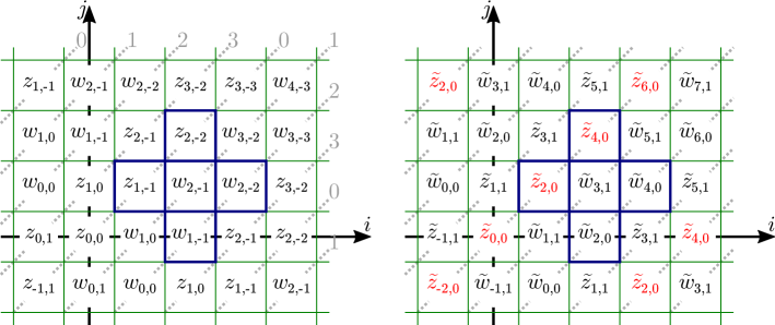
Figure 10: Face weights for the explicit solution of Bäcklund pairs in Theorem 5.4 (left). The dotted diagonals correspond to constant values of $[i-j]_{4}$, with that value indicated at the end. The sample blue Aztec diamond corresponds to the computation of $z_{3,0}$. Right: the same values after the change of variable (5.8). Variables in red are those that are set to $0$ in Theorem 5.7.

Theorem 5.4.

Let $z,w:\mathbb{Z}^{2}\rightarrow\hat{\mathbb{C}}$ be a Bäcklund pair of integrable cross-ratio maps, and consider the graph $\mathbb{Z}^{2}$ with face weights $(a_{i,j})_{(i,j)\in\mathbb{Z}^{2}}$ given by,

$$a_{i,j}=\begin{cases}z_{\frac{i+j+[i+j]_{2}}{2},\frac{-(i+j)+[i+j]_{2}}{2}}&\text{ if }[i-j]_{4}\in\{0,3\},\\ w_{\frac{i+j+[i+j]_{2}}{2},\frac{-(i+j)+[i+j]_{2}}{2}}&\text{ if }[i-j]_{4}\in\{1,2\}.\end{cases}$$

Then, for all $(i,j)\in\mathbb{Z}^{2}$ such that $i+j\geq 1$, introducing the notation

$$(i^{\prime},j^{\prime}):=\Bigl{(}\frac{i-j+[i-j]_{2}}{2},\frac{-(i-j)+[i-j]_{2}}{2}\Bigr{)},$$

we have

$$z_{i,j} =\begin{cases}Y(A_{i+j-1}[z_{i^{\prime},j^{\prime}}],a)&\text{ if $[i+j]_{4}\in\{0,1\}$},\\ Y(A_{i+j-1}[w_{i^{\prime},j^{\prime}}],a)&\text{ if $[i+j]_{4}\in\{2,3\}$},\end{cases}$$

$$w_{i,j} =\begin{cases}Y(A_{i+j-1}[z_{i^{\prime},j^{\prime}}],a)&\text{ if $[i+j]_{4}\in\{2,3\}$},\\ Y(A_{i+j-1}[w_{i^{\prime},j^{\prime}}],a)&\text{ if $[i+j]_{4}\in\{0,1\}$.}\end{cases}$$

Proof.

Consider the function $x:\mathcal{L}\rightarrow\hat{\mathbb{C}}$ given by

$$x(i,j,k)=\begin{cases}z_{\frac{i+j+k}{2},\frac{-(i+j)+k}{2}}&\mbox{ for }[i-j+k]_{4}=0,\\ w_{\frac{i+j+k}{2},\frac{-(i+j)+k}{2}}&\mbox{ for }[i-j+k]_{4}=2.\end{cases}$$ (5.4)

As a consequence of Lemma 5.3, we have that, for all $(i,j)\in\mathbb{Z}^{2}$, and all $k\geq 1$, the function $x$ satisfies the dSKP recurrence. Consider $(i,j)\in\mathbb{Z}^{2}$, such that $[i-j]_{4}\in\{0,3\}$ (the argument when $[i-j]_{4}\in\{1,2\}$ is similar), then $[i-j+[i+j]_{2}]_{4}=[i-j+[i-j]_{2}]=0$, and the function $x$ satisfies the initial condition

$$a_{i,j}=x(i,j,[i+j]_{2})=z_{\frac{i+j+[i+j]_{2}}{2},\frac{-(i+j)+[i+j]_{2}}{2}},$$

giving the face weights of the statement. As a consequence of Theorem 2.2, we know that $x(i,j,k)=Y(A_{k-1}[a_{i,j}],a)$. Using Equation (5.4), we have that for every $m\in\mathbb{Z}$,

$$x(m,i-j-m,i+j)=\begin{cases}z_{i,j}&\text{ if $m+j\in 2\mathbb{Z}$},\\ w_{i,j}&\text{ if $m+j\in 2\mathbb{Z}+1$}.\end{cases}$$ (5.5)

Applying this at $m=j$, we get that $z_{i,j}=x(j,i-2j,i+j)=Y(A_{i+j-1}[a_{j,i-2j}])$. An explicit computation of the face weight $a_{j,i-2j}$ gives

• if $[-i+3j]_{4}\in\{0,3\}$ (which is equivalent to $[-i-j]_{4}\in\{0,3\}$, or $[i+j]_{4}\in\{0,1\}$), then $a_{j,i-2j}=z_{i^{\prime},j^{\prime}}$.

• if $[-i+3j]_{4}\in\{1,2\}$ (which is equivalent to $[-i-j]_{4}\in\{1,2\}$, or $[i+j]_{4}\in\{2,3\}$), then $a_{j,i-2j}=w_{i^{\prime},j^{\prime}}$.

This shows that $z_{i,j}$ is the ratio of partition functions of the Aztec diamond of size $i+j-1$ centered at $(j,i-2j)$, whose central face has weight $z_{i^{\prime},j^{\prime}}$. However, note that the whole solution (5.4) is invariant under translations of multiples of $(2,-2,0)$. Therefore, any Aztec diamond of size $i+j-1$ whose central face has weight $z_{i^{\prime},j^{\prime}}$ is a translate of the first one by such a translation, and has the same face weights and ratio of partition functions. As a consequence, it is not important that the Aztec diamond is centered at $(j,i-2j)$, but only that it has the announced central face weight.

Doing the same for $m=j+1$ gives the expression of $w_{i,j}$. ∎

Remark 5.5.

Due to the definition of integrable cross-ratio maps it is possible to express $(z_{i,j})_{i+j>1}$ in terms of $(z_{i,j})_{i+j\in\{0,1\}}$ and $(\alpha_{i},\beta_{j})_{i,j\in\mathbb{Z}}$. However, these expressions can become arbitrarily complicated rational functions, so this is not in the spirit of giving explicit combinatorial expressions. It would be interesting to find an explicit combinatorial expression for the data of $z$ only in terms of $(z_{i,j})_{i+j\in\{0,1\}}$ and $(\alpha_{i},\beta_{j})_{i,j\in\mathbb{Z}}$, without resorting to a Bäcklund partner $w$.

5.3 Dual map

The following construction helps both in the proof and the statement of singularities. Given an integrable cross-ratio map, we define the discrete 1-form ${\mathrm{d}}{z}(v,v^{\prime})=z(v^{\prime})-z(v)$ for any two adjacent $v,v^{\prime}\in\mathbb{Z}^{2}$. This 1-form is closed by construction. Additionally, we consider the dual discrete 1-form ${\mathrm{d}}{z^{*}}$ given by

$${\mathrm{d}}{z^{*}}((i,j),(i+1,j)) =\frac{\alpha_{i}}{z_{i,j}-z_{i+1,j}}, {\mathrm{d}}{z^{*}}((i,j),(i,j+1)) =\frac{\beta_{j}}{z_{i,j}-z_{i,j+1}}.$$ (5.6)

This 1-form is also closed [BP96, Theorem 6]; this follows from the the cross-ratio condition of Definition 5.1. Any map $z^{*}$ obtained by integrating ${\mathrm{d}}{z^{*}}$ is called a dual map to $z$. Additionally, assume $z,w$ are a Bäcklund pair. By employing the cross-ratio conditions of Definition 5.2 we may moreover assume that the dual maps $z^{*},w^{*}$ satisfy $w^{*}-z^{*}=\gamma(z-w)^{-1}$. We may see $z^{*}$ (resp. $w^{*}$) as defined on the plane at height $0$ (resp. $1$) in $\mathbb{Z}^{3}$ as in Figure 9, so the previous formula gives vertical increments. Finally, the following identity [BS02, Section 5.4]

$${\mathrm{d}}{z^{*}}((i+1,j),(i,j))+{\mathrm{d}}{z^{*}}((i,j),(i,j+1))=\frac{\alpha_{i}}{z_{i+1,j}-z_{i,j}}+\frac{\beta_{j}}{z_{i,j}-z_{i,j+1}}=\frac{\alpha_{i}-\beta_{j}}{z_{i+1,j+1}-z_{i,j}},$$ (5.7)

is called the three-legged form and is useful in some of the upcoming calculations.

5.4 Change of coordinates

The following change of coordinates helps to better outline the structure of the data. It is also useful to describe singularities in Section 5.5. For $(i,j)\in\mathbb{Z}^{2}$, let

$$z_{i,j}=\tilde{z}_{i-j,i+j},$$ (5.8)

and let $\tilde{z}_{j}=(\tilde{z}_{i,j})_{[i+j]_{2}=0}$, noting that $\tilde{z}_{i,j}$ is only defined for $i+j\in 2\mathbb{Z}$. We will use the tilde to signify this change of coordinates in the remainder of the paper. The inverse coordinate transform is

$$\tilde{z}_{i,j}=z_{\frac{i+j}{2},\frac{-i+j}{2}}.$$ (5.9)

An example is provided in Figure 10.

Remark 5.6.

In the rotated coordinates, the explicit expression of Theorem 5.4 takes the following simpler form: for all $(i,j)\in\mathbb{Z}^{2}$ such that $[i+j]_{2}=0$,

$$\tilde{z}_{i,j}=\begin{cases}Y(A_{j-1}[\tilde{z}_{i,[i]_{2}}],a)&\text{ if $[j]_{4}\in\{0,1\}$},\\ Y(A_{j-1}[\tilde{w}_{i,[i]_{2}}],a)&\text{ if $[j]_{4}\in\{2,3\}$},\end{cases}\quad\quad\tilde{w}_{i,j}=\begin{cases}Y(A_{j-1}[\tilde{z}_{i,[i]_{2}}],a)&\text{ if $[j]_{4}\in\{2,3\}$},\\ Y(A_{j-1}[\tilde{w}_{i,[i]_{2}}],a)&\text{ if $[j]_{4}\in\{0,1\}$.}\end{cases}$$

5.5 Singularities

We now turn to studying singularities of integrable cross ratio maps. If we know $\tilde{z}_{j}$, $\tilde{z}_{j+1}$ and the functions $\alpha$ and $\beta$, then by Definition 5.1, we also know $\tilde{z}_{j+2}$. Let us denote by $T$ the map representing the propagation of data

$$T:(\hat{\mathbb{C}})^{\mathbb{Z}_{2}\times\mathbb{Z}}\rightarrow(\hat{\mathbb{C}})^{\mathbb{Z}_{2}\times\mathbb{Z}},\quad(\tilde{z}_{j},\tilde{z}_{j+1})\mapsto(\tilde{z}_{j+1},\tilde{z}_{j+2}).$$

Let $m\geq 1$. An integrable cross-ratio map $z$ is said to be $m$-periodic if $\alpha_{i}=\alpha_{i+m}$, $\beta_{i}=\beta_{i+m}$, and $z_{i,j}=z_{i+m,j-m}$ for all $(i,j)\in\mathbb{Z}^{2}$; the last condition is equivalent to $\tilde{z}_{i+2m,j}=\tilde{z}_{i,j}$ for all $(i,j)\in\mathbb{Z}^{2}$ such that $[i+j]_{2}=0$. A dual map $z^{*}$ to a periodic map $z$ is not necessarily periodic, instead $z^{*}$ has an additive monodromy $M[z^{*}]=z^{*}_{i+m,j-m}-z^{*}_{i,j}$ that does not depend on $i,j$ or the choice of dual map $z^{*}$. A Bäcklund pair of integrable cross-ratio maps $z,w$ is called $m$-periodic if both $z$ and $w$ are $m$-periodic. We claim that generically, for a given $m$-periodic integrable cross-ratio map $z$ there exists an integrable cross-ratio map $w$, such that $z,w$ is an $m$-periodic Bäcklund pair. Recall that we explained how to construct a Bäcklund pair from $w$ in the non-periodic case in Section 5.1. In the periodic case, assume we begin by setting $\tilde{w}_{0,0}=\hat{w}$ for some formal variable $\hat{w}$. Then we iteratively express $\tilde{w}_{1,1},\tilde{w}_{2,0},\tilde{w}_{3,1},\tilde{w}_{4,0},\dots,\tilde{w}_{2m,0}$ as Möbius transforms of $\hat{w}$. As a Möbius transform generically has two fixed points, we can choose $\hat{w}$ to equal one of the fixed points. The remainder of $\tilde{w}$ is determined by the propagation $T$ and thus we have constructed an $m$-periodic Bäcklund pair.

We prove the following singularity result.

Theorem 5.7.

Let $m\geq 1$, and let $\tilde{z}$ be an $m$-periodic integrable cross-ratio map such that $\tilde{z}_{i,0}=0$ for all $i\in 2\mathbb{Z}$. Assume we can apply the propagation map $T$ to $(\tilde{z}_{0},\tilde{z}_{1})$ at least $2m-2$ times. Then for all $i\in 2\mathbb{Z}+1$,

$$\tilde{z}_{i,2m-1}=\frac{\sum_{\ell=0}^{m-1}\left(\alpha_{\ell}-\beta_{\ell}\right)}{\sum_{\ell=0}^{m-1}\frac{1}{\tilde{z}_{2\ell+1,1}}\left(\alpha_{\ell}-\beta_{-\ell-1}\right)}=\frac{1}{M[z^{*}]}\sum_{\ell=0}^{m-1}\left(\alpha_{\ell}-\beta_{\ell}\right).$$ (5.10)

Remark 5.8.

Prior to proving the theorem, let us mention again that this may be seen as an equality on rational functions of formal variables $\alpha,\beta$ and $\tilde{z}_{1}$. Thus we may assume that there is an $\ell$ such that $\alpha_{\ell}\neq\beta_{-\ell-1}$, indeed, when this is not the case, the conclusion of the theorem (taken as a formal expression specified to that case) shows that $\tilde{z}_{i,2m-1}$ is undefined, so the propagation map $T$ could not, in fact, be applied $2m-2$ times.

Proof.

Note that the right equality follows immediately from the definition of the monodromy $M[z^{*}]$ of the dual 1-form.

Let $\tilde{w}$ be an $m$-periodic integrable cross-ratio map such that $\tilde{z},\tilde{w}$ is a Bäcklund pair with $\gamma=1$.

The initial condition in the claim is a case of $(m,2)$-Devron initial condition, see Figure 10. Therefore, by Theorem 2.8, we know that for the corresponding solution of the dSKP recurrence, if $[i-j-2m]_{4}=0$ then $x(i,j,2m-2)=x(i+1,j+1,2m-2)$. This solution is also explicitly described in (5.4), and noting that in this case $[i-j+(2m-2)]_{4}=2$, the previous equation becomes

$$w_{\frac{i+j}{2}+m-1,\frac{-(i+j)}{2}+m-1}=w_{\frac{i+j}{2}+m,\frac{-(i+j)}{2}+m-2},$$

or equivalently, $\tilde{w}_{i+j,2m-2}=\tilde{w}_{i+j+2,2m-2}$. In other words, $\tilde{w}_{2m-2}$ is constant. Generally, if $\tilde{w}_{i,j}=\tilde{w}_{i+2,j}\neq\tilde{w}_{i+1,j-1}$ then $\tilde{w}_{i+1,j+1}$ is not defined by Equation (5.1). However, if $\tilde{z}_{i,j},\tilde{z}_{i+2,j},\tilde{z}_{i+1,j-1}$ are pairwise different and different from $\tilde{w}_{i,j},\tilde{w}_{i+2,j},\tilde{w}_{i+1,j-1}$ then $\tilde{z}_{i+1,j+1}$ is defined and equal to $\tilde{w}_{i,j}$. As a consequence, $\tilde{z}_{2m-1}$ is constant.

We now compute this constant, for which we choose to compute $\tilde{w}_{2m-2,2m-2}$ using Theorem 2.3. The corresponding Aztec diamond has size $2m-3$, and its weights can be obtained from the previous solution of dSKP; a quick check shows that they are those of Figure 11. Let $D$ be the corresponding operator as in the discussion preceding Theorem 2.3, and let $v\in\mathbb{C}^{F}$ be a nonzero element of $\ker D^{T}$, which exists by a dimension argument.

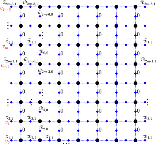
Figure 11: The weights on the graph defining $D$ in the case of a $m$-periodic Bäcklund pair with $\tilde{z}_{0}\equiv 0$. The same $4$ columns of weights repeat throughout the graph. In particular there are $m-1$ columns with weights $0$.

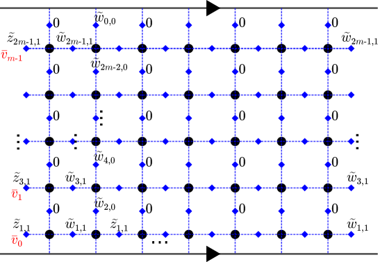
Figure 12: The graph on a cylinder obtained from that of Figure 11 by quotienting the $m$-periodicity.

Consider the graph on a cylinder obtained by a $(0,m)$ quotient of the previous graph, inheriting the face weights consistently, see Figure 12; we denote its black vertices by $\bar{B}$, its faces by $\bar{F}$, and the corresponding operator from $\mathbb{C}^{\bar{B}}\oplus\mathbb{C}^{\bar{B}}$ to $\mathbb{C}^{\bar{F}}$ by $\bar{D}$. Each element of $\bar{F}$ corresponds to one or two elements of $F$. By summing the entries of $v$ from these one or two elements, we get a vector $\bar{v}\in\mathbb{C}^{\bar{F}}$. It is easy to see that $\bar{v}\in\ker\bar{D}^{T}$. Note also that the weighted sums of the leftmost entries of $v$, as in Theorem 2.3, can be computed from $\bar{v}$, using the periodicity of $\tilde{z}_{1}$:

$$\begin{split}\sum_{\ell=0}^{2m-3}v_{\ell}&=\sum_{\ell=0}^{m-1}\bar{v}_{\ell},\\ \sum_{\ell=0}^{2m-3}a_{\ell}v_{\ell}&=\sum_{\ell=0}^{2m-3}\tilde{z}_{2\ell+1,1}v_{\ell}=\sum_{\ell=0}^{m-1}\tilde{z}_{2\ell+1,1}\bar{v}_{\ell}.\end{split}$$ (5.11)

If $\bar{v}\equiv 0$, then these two sums are $0$, and by Theorem 2.3, $\tilde{w}_{2m-2,2m-2}$ is undefined, which means that for these initial conditions the map $T$ cannot be applied $2m-2$ times. We now suppose that $\bar{v}$ is not the zero vector.

We have $|\bar{F}|=2|\bar{B}|+m$, so $\dim\ker\bar{D}^{T}\geq m$. We will show that this dimension is in fact $m$ and provide a basis of $\ker\bar{D}^{T}$, which we will use to get information on $\bar{v}$. First, for each of the $m-1$ columns of zeros in the quotient graph, we can put ones on this whole column, and zeros everywhere else; it is easy to check that this gives $m-1$ free vectors in $\ker\bar{D}^{T}$. The $m$-th vector we introduce has the following entries:

• on each element of $\bar{F}$ carrying a weight $\tilde{z}_{2\ell+1,1}$, the entry is $\frac{\alpha_{\ell}-\beta_{-\ell-1}}{\tilde{z}_{2\ell+1,1}}$;

• on each element of $\bar{F}$ carrying a weight $\tilde{w}_{2\ell+1,1}$, the entry is $\frac{\alpha_{\ell}-\beta_{-\ell-1}}{\tilde{w}_{2\ell+1,1}}$;

• on each element of $\bar{F}$ carrying a weight $\tilde{w}_{2\ell,0}$, the entry is $\frac{-1}{\tilde{w}_{2\ell,0}}$;

• on each element of $\bar{F}$ carrying a weight $0$ and on the same row as $\tilde{w}_{2\ell,0}$, the entry is $\frac{-1}{\tilde{w}_{2\ell,0}}$.

By Remark 5.8, this is not in the span of the previous $m-1$ vectors. We now check that this indeed defines a vector in $\ker\bar{D}^{T}$, which means we have to check two linear conditions for each element of $\bar{B}$. By periodicity of the vector, we just have to check it for the first two columns of $\bar{B}$. On the first column at row $\ell$, the first relation to check is

$$\frac{\alpha_{\ell}-\beta_{-\ell-1}}{\tilde{w}_{2\ell+1,1}}+\frac{-1}{\tilde{w}_{2\ell+2,0}}=\frac{\alpha_{\ell}-\beta_{-\ell-1}}{\tilde{z}_{2\ell+1,1}}+\frac{-1}{\tilde{w}_{2\ell,0}}.$$ (5.12)

Recall that $\tilde{z}_{2\ell,0},\tilde{z}_{2\ell+2,0}$ are zero, so that we may assume that $\tilde{w}_{2\ell+1,-1}$ is zero as well; a short computation shows that (5.1) still holds for $w$. Moreover, applying Equation (5.7) for $w$ at $i=\ell,j=-\ell-1$, we obtain

$$\frac{\alpha_{\ell}-\beta_{-\ell-1}}{\tilde{w}_{2\ell+1,1}}=\frac{\alpha_{\ell}}{\tilde{w}_{2\ell+2,0}}-\frac{\beta_{-\ell-1}}{\tilde{w}_{2\ell,0}}.$$ (5.13)

Substituting this expression into Equation (5.12), we obtain the integral of the dual 1-form along the closed path corresponding to $\tilde{z}_{2\ell,0},\tilde{w}_{2\ell,0},\tilde{w}_{2\ell+1,-1},\tilde{w}_{2\ell+2,0},\tilde{z}_{2\ell+2,0},\tilde{z}_{2\ell+1,1},\tilde{z}_{2\ell,0}$. Thus Equation (5.12) follows from the fact that the dual 1-form is closed.

The second condition for the first column is

$$\tilde{w}_{2\ell+1,1}\times\frac{\alpha_{\ell}-\beta_{-\ell-1}}{\tilde{w}_{2\ell+1,1}}+0\times\frac{-1}{\tilde{w}_{2\ell+2,0}}=\tilde{z}_{2\ell+1,1}\times\frac{\alpha_{\ell}-\beta_{-\ell-1}}{\tilde{z}_{2\ell+1,1}}+0\times\frac{-1}{\tilde{w}_{2\ell,0}},$$ (5.14)

which is trivial. We now turn to the second column. The first condition is again (5.12). The second condition is

$$\tilde{w}_{2\ell+1,1}\times\frac{\alpha_{\ell}-\beta_{-\ell-1}}{\tilde{w}_{2\ell+1,1}}+\tilde{w}_{2\ell+2,0}\times\frac{-1}{\tilde{w}_{2\ell+2,0}}=\tilde{z}_{2\ell+1,1}\times\frac{\alpha_{\ell}-\beta_{-\ell-1}}{\tilde{z}_{2\ell+1,1}}+\tilde{w}_{2\ell,0}\times\frac{-1}{\tilde{w}_{2\ell,0}},$$ (5.15)

which is also trivial.

Thus we have found $m$ free vectors in $\ker\bar{D}^{T}$. We claim that this space has dimension $m$. Indeed, if its dimension was higher, using the rank-nullity theorem we would have $\dim\ker\bar{D}\geq 1$, so there would be a nonzero vector $\bar{u}\in\mathbb{C}^{\bar{B}}\oplus\mathbb{C}^{\bar{B}}$ in this subspace. By putting the same entries as those of $\bar{u}$ on the initial graph, we would get a nonzero vector $u\in\mathbb{C}^{B}\oplus\mathbb{C}^{B}$, and it is easy to see that $u\in\ker D$. By the rank-nullity theorem again, this implies that $\dim\ker D^{T}\geq 2$. Using Proposition 2.4, this implies again that the map $T$ could not be applied $2m-2$ times.

Therefore, $\bar{v}$ is a combination of the $m$ vectors we described. This implies that there is a constant $\lambda$ such that $(\bar{v}_{\ell})_{0\leq\ell\leq m-1}=\lambda\ (\frac{\alpha_{\ell}-\beta_{-\ell-1}}{\tilde{z}_{2\ell+1,1}})_{0\leq\ell\leq m-1}$. By (5.11) and Theorem 2.3, this gives the claimed value; note that if $\lambda=0$, again the ratio is not defined and we conclude as before. ∎

Remark 5.9.

Let us write $S[\alpha,\beta]:=\sum_{\ell=0}^{m-1}(\alpha_{\ell}-\beta_{\ell})$. Assuming $\tilde{z}$ is $m$-periodic and singular, in the sense that $\tilde{z}_{0}$ is constant, Theorem 5.7 states that

$$\tilde{z}_{2m-1}-\tilde{z}_{0}=\frac{S[\alpha,\beta]}{M[z^{*}]}.$$ (5.16)

Thus there is a simple relation between the positions of the two singularities and the additive monodromy of $z^{*}$. Moreover, note that $z^{*}$ features a repeating singularity as well. In particular, one can immediately verify that $\tilde{z}^{*}_{-1}=\tilde{z}^{*}_{2m}\equiv\infty$. It would be interesting to understand if and how singularity theorems also hold in more general setups when $z$ is only quasi-periodic.

6 Discrete holomorphic functions and orthogonal circle patterns

6.1 Definitions and relation to Bäcklund pairs

There are different kinds of maps that are considered to be discretizations of holomorphic functions in the literature [BMS05, CLR20, Duf56, Ken02, Sch97, Smi10, Ste02] . The definition we use here is due to Bobenko and Pinkall [BP96] and independently Nijhoff and Capel [NC95]. It is a specific instance of an integrable cross-ratio map when $\alpha_{i}\equiv-\mu,\beta_{j}\equiv\mu^{-1}$ for some $\mu\in\mathbb{C}\setminus\{0\}$, although without loss of generality we assume $\mu=1$ and therefore $\alpha_{i}\equiv-1,\beta_{j}\equiv 1$. These discrete holomorphic functions are also solutions to the discrete KdV equation [KS02, Section 5].

Definition 6.1.

A discrete holomorphic function is a map $z:\mathbb{Z}^{2}\rightarrow\hat{\mathbb{C}}$ such that, for every quad of $\mathbb{Z}^{2}$, the following holds

$$\operatorname{cr}(z_{i,j},z_{i+1,j},z_{i+1,j+1},z_{i,j+1})=-1.$$ (6.1)

Recall that for a given $\gamma$ and a given point in $\mathbb{C}$, there is a unique integrable cross ratio map $w$ such that $z,w$ is a Bäcklund pair. A useful fact is that, in the specific case of discrete holomorphic functions, this can be carried out explicitly as stated by the following.

Lemma 6.2.

Consider a discrete holomorphic function $z:\mathbb{Z}^{2}\rightarrow\hat{\mathbb{C}}$. Set $\gamma=1$, and for a given $(i^{\prime},j^{\prime})\in\mathbb{Z}^{2}$, set $w_{i^{\prime},j^{\prime}}=z_{i^{\prime},j^{\prime}+1}$. Then, the discrete holomorphic function $w:\mathbb{Z}^{2}\rightarrow\hat{\mathbb{C}}$ such that $z,w$ is a Bäcklund pair is explicitly given by, for all $(i,j)\in\mathbb{Z}^{2}$,

$$w_{i,j}=z_{i,j+1}.$$ (6.2)

Proof.

The proof consists in a explicit reconstruction of $w$ starting from the point $w_{i^{\prime},j^{\prime}}=z_{i^{\prime},j^{\prime}+1}$ using Definition 5.2 as described in Section 5.1. ∎

Using Lemma 6.2, we now state the dSKP relation given by Lemma 5.3 in the setting of discrete holomorphic functions, thus recovering a result of [KS02, Section 5].

Corollary 6.3.

Let $z$ be a discrete holomorphic function. Then, the following equation holds for all $(i,j)\in\mathbb{Z}^{2}$,

$$\frac{(z_{i,j}-z_{i+1,j})(z_{i+1,j+1}-z_{i+1,j+2})(z_{i,j+2}-z_{i,j+1})}{(z_{i+1,j}-z_{i+1,j+1})(z_{i+1,j+2}-z_{i,j+2})(z_{i,j+1}-z_{i,j})}=-1.$$ (6.3)

6.2 Explicit solution

We now apply Theorem 5.4 to the Bäcklund pair $z,w$ corresponding to holomorphic functions thus giving an explicit expression for $z_{i,j}$ for all $(i,j)\in\mathbb{Z}^{2}$ such that $i+j\geq 1$, as a function of $(z_{i^{\prime},j^{\prime}})_{i^{\prime}+j^{\prime}\in\{0,1,2\}}$. Observe that Theorem 5.4 gives two ways of expressing $z_{i,j}$: one using $z_{i,j}$ of course, and the other using $z_{i,j}=w_{i,j-1}$. As a consequence, $z_{i,j}$ can be expressed using an Aztec diamond of size $i+j-1$ or $i+j-2$; we use the second way in Corollary 6.4 below since the Aztec diamond is smaller. Note that one can also see on the level of combinatorics that the two ways are consistent: some edges of the Aztec diamond can be removed, which impose some edges to be present on the boundary, and allow to reduce the size of the Aztec diamond by one in the case where we use the one having size $i+j-1$, see also Remark 6.5. An illustration of Corollary 6.4 is given in Figure 13.

Corollary 6.4.

Let $z:\mathbb{Z}^{2}\rightarrow\hat{\mathbb{C}}$ be a discrete holomorphic function, and consider the graph $\mathbb{Z}^{2}$ with face weights $(a_{i,j})_{(i,j)\in\mathbb{Z}^{2}}$ given by,

$$a_{i,j}=\begin{cases}z_{\frac{i+j+[i+j]_{2}}{2},\frac{-(i+j)+[i+j]_{2}}{2}}&\text{ if }[i-j]_{4}\in\{0,3\},\\ z_{\frac{i+j+[i+j]_{2}}{2},\frac{-(i+j)+[i+j]_{2}}{2}+1}&\text{ if }[i-j]_{4}\in\{1,2\}.\end{cases}$$

Then, for all $(i,j)\in\mathbb{Z}^{2}$ such that $i+j\geq 2$, we have

$$z_{i,j} =\begin{cases}Y(A_{i+j-2}[z_{i^{\prime},(j-1)^{\prime}}],a)&\text{ if $[i+j]_{4}\in\{0,3\}$},\\ Y(A_{i+j-2}[z_{i^{\prime},(j-1)^{\prime}+1}],a)&\text{ if $[i+j]_{4}\in\{1,2\}$.}\end{cases}$$

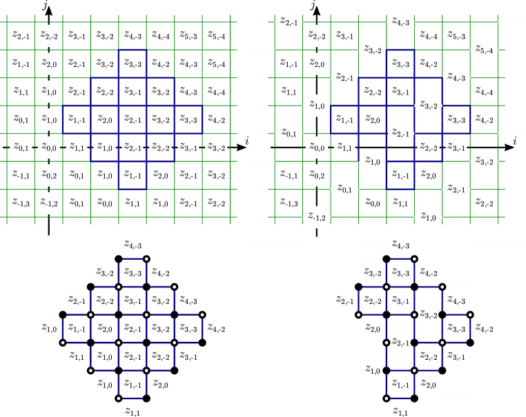
Figure 13: Face weights for the explicit solution of discrete holomorphic functions. Top left: face weights deduced from the Bäcklund pair case with $w_{i,j}=z_{i,j+1}$. Top right: graph obtained after removing edges of resulting dimer weight $0$. Bottom left: Aztec diamond of size $3$ used to compute $z_{4,1}$, using $w_{4,0}$ in the Bäcklund pair case. Bottom right: graph with the same ratio of partition functions, obtained from the Aztec diamond via the existence of forced dimers.

Remark 6.5.

There are pairs of diagonals with identical weights. Returning to the definition of the oriented dimer partition function, an edge separating two squares with the same face has two possible orientations that cancel each other, and can thus be removed. As a consequence, in this case, the lattice $\mathbb{Z}^{2}$ can be transformed into a lattice consisting of a repeating pattern of pairs of diagonals of squares, followed by a diagonal of hexagons, see Figure 13. One can also obtain this resulting graph made of hexagons and squares via the method of crosses and wrenches, using the solution to the dSKP recurrence associated to the height function of an initial condition different than $[i+j]_{2}$. This method was developed by Speyer for the dKP recurrence [Spe07], and extended to the dSKP recurrence in [AdTM22, Section 2].

6.3 Discrete holomorphic functions and P-nets

We now explain a connection between discrete holomorphic functions and P-nets. This link provides an alternative explicit expression for $z_{i,j}$, and is also of use in the next section on singularities.

Let $\mathbb{Z}^{2}_{\pm}$ denote the even and odd sublattices $\{(i,j)\in\mathbb{Z}^{2}:(-1)^{i+j}=\pm 1\}$, where we consider two vertices in $\mathbb{Z}_{\pm}^{2}$ to be adjacent if they are at graph distance 2 in $\mathbb{Z}^{2}$.

Consider a discrete holomorphic function $z:\mathbb{Z}^{2}\rightarrow\hat{\mathbb{C}}$, written in the rotated coordinates $(\tilde{z}_{i,j})_{[i+j]_{2}=0}$ given by Equation (5.8). Let $p$ be the restriction of $\tilde{z}$ to $\mathbb{Z}^{2}_{+}$, and $q$ the restriction to $\mathbb{Z}^{2}_{-}$, i.e., for all $(i,j)\in\mathbb{Z}^{2}$,

$$\begin{split}p_{i,j}&=\tilde{z}_{2i,2j}=z_{i+j,-i+j},\\ q_{i,j}&=\tilde{z}_{2i+1,2j+1}=z_{i+j+1,-i+j}.\end{split}$$ (6.4)

Then, we have the following.

Lemma 6.6.

([BP99, Lemma 6]) Let $z:\mathbb{Z}^{2}\rightarrow\hat{\mathbb{C}}$ be a discrete holomorphic function. Then both $p$ and $q$ are P-nets. Conversely, given a P-net $p$ there is a (complex) one-parameter family of P-nets $q^{\prime}$ such that $p$ and $q^{\prime}$ together are a discrete holomorphic function.

Question 6.7.

As a consequence of Lemma 6.6 one can use the P-net explicit solution of Theorem 4.3 to give an explicit expression of $z_{i,j}$, separating the even and odd cases. It is striking to see that the Aztec diamond with this approach is typically only half the size of the one given by Corollary 6.4. At this stage we do not understand how to prove directly that the ratio partition functions of these two Aztec diamonds are equal, and pose this as an intriguing open question.

6.4 Singularities

In this section, we study singularities of discrete holomorphic functions. The first part consists in writing down the integrable cross ratio/Bäcklund pairs result (Theorem 5.7) in the specific case of discrete holomorphic functions, thus recovering a result of [Yao14]. Next, using the connection between discrete holomorphic functions and P-nets, we provide an alternative proof of this result, as well as a refined version thereof.

6.4.1 Immediate consequences

Recall the definition of the map $T$ describing the propagation of data

$$T:(\hat{\mathbb{C}})^{\mathbb{Z}_{2}\times\mathbb{Z}}\rightarrow(\hat{\mathbb{C}})^{\mathbb{Z}_{2}\times\mathbb{Z}},\quad(\tilde{z}_{j},\tilde{z}_{j+1})\mapsto(\tilde{z}_{j+1},\tilde{z}_{j+2}).$$

Let $m\geq 1$. A discrete holomorphic function $z$ is said to be m-periodic if it is $m$-periodic as integrable cross-ratio map, that is if $z_{i,j}=z_{i+m,j-m}$ for all $(i,j)\in\mathbb{Z}^{2}$, or equivalently $\tilde{z}_{i+2m,j}=\tilde{z}_{i,j}$ for all $i,j\in\mathbb{Z}$ such that $[i+j]_{2}=0$. Then, using that $\alpha_{i}\equiv-1$, $\beta_{j}\equiv 1$, Theorem 5.7 becomes  [Yao14, Theorem 1.5].

Corollary 6.8 ([Yao14]).

Let $m\geq 1$, and let $\tilde{z}$ be an $m$-periodic discrete holomorphic function such that $\tilde{z}_{i,0}=0$ for all $i\in 2\mathbb{Z}$. Assume we can apply the propagation map $T$ to $(\tilde{z}_{0},\tilde{z}_{1})$ at least $2m-2$ times. Then, for all $i\in 2\mathbb{Z}+1$,

$$\tilde{z}_{i,2m-1}=\Bigl{(}\frac{1}{m}\sum_{\ell=0}^{m-1}\frac{1}{\tilde{z}_{2\ell+1,1}}\Bigr{)}^{-1},$$

that is $\tilde{z}_{2m-1}$ is constant with value equal to the harmonic mean of $\tilde{z}_{1}$.

6.4.2 Further singularity results

Let us prove a preliminary lemma.

Lemma 6.9.

Let $m\in 2\mathbb{N}+2$, let $z:\mathbb{Z}^{2}\rightarrow\hat{\mathbb{C}}$ be an $m$-periodic discrete holomorphic function such that, for all $i\in\mathbb{Z}$, $z_{i,-i}=0$, and let $p,q$ be the associated P-nets. Then

$$\sum_{i=0}^{m-1}\frac{(-1)^{i}}{p_{i,1}}=0.$$

Proof.

Using $\alpha_{i}\equiv-1$, $\beta_{j}\equiv 1$, and $z_{i,-i}=0$, Equation (5.7) becomes

$$\frac{{-1}}{-z_{i,-i+1}}+\frac{1}{z_{i+1,-i}}=\frac{2}{z_{i+1,-i+1}}.$$

Therefore, using the relation between P-nets and holomorphic functions (6.4), the claim becomes

$$\sum_{i=0}^{m-1}\frac{(-1)^{i}}{2}\left(\frac{{1}}{z_{i,-i+1}}+\frac{1}{z_{i+1,-i}}\right)=0,$$

which is clearly true because of the periodicity of $z$ and the fact that $m$ is even.∎

We are now ready to state our refined singularity result. More precisely, we reprove that for $m$ odd, $\tilde{z}_{2m-1}$ is indeed identically equal to this harmonic mean, while for $m$ even, we show that $\tilde{z}_{2m-2}$ is in fact already identically equal to this harmonic mean, i.e., the singularity appears one step earlier than predicted by Yao. Note that this is not a contradiction, it just means that the map $T$ cannot be iterated $2m-2$ times.

Figure 14: Propagation of discrete holomorphic functions with an initial singularity at the black point. Left: 3-periodic case, which degenerates after 4 steps. Center and right: 4-periodic case, which degenerates generically after 5 steps (center), and in special cases after 4 steps (right).

Theorem 6.10 ([Yao14] ($m$ odd)).

Let $m\geq 1$ and let $n=2m-2$ if $m$ is odd, and $n=2m-3$ if $m$ is even. Let $\tilde{z}$ be an $m$-periodic discrete holomorphic function such that $\tilde{z}_{i,0}=0$ for all $i\in 2\mathbb{Z}$. Assume we can apply the propagation map $T$ to $(\tilde{z}_{0},\tilde{z}_{1})$ at least $n$ times. Then, for all $i\in\mathbb{Z}$ such that $[i+n+1]_{2}=0$, we have

$$\tilde{z}_{i,n+1}=\left(\frac{1}{m}\sum_{\ell=0}^{m-1}\frac{1}{\tilde{z}_{2\ell+1,1}}\right)^{-1}.$$

In other words, $\tilde{z}_{n+1}$ is constant with value equal to the harmonic mean of $\tilde{z}_{1}$.

Proof.

Consider the P-nets $p,q$ associated to $z$, where $p,q$ are defined on $\{(i,j)\in\mathbb{Z}^{2}:j\geq 0\}$. The row $p_{0}$ corresponds to the singular initial row that is mapped to 0, see Figure 15. We consider the case of odd $m$ first. Define a map $r$ on $\{(i,j)\in\mathbb{Z}^{2}:j\geq-1\}$ as a continuation of $q$ by

$$r_{i,j}=\begin{cases}q_{i,j}&j\geq 0,\\ 0&j=-1.\end{cases}$$

A small calculation shows that $r$ satisfies the P-net condition of Definition 4.1 also in row $0$, where the calculation uses that $r_{1}=\tilde{z}_{3}$ is completely determined by $p_{0}=\tilde{z}_{0},r_{0}=\tilde{z}_{1}$ via the propagation of discrete holomorphic functions. Thus $r$ is also a P-net. Therefore, we can apply Theorem 4.4 to $r$ and obtain that $z$ is singular after $2m-2$ iterations of discrete holomorphic propagation, becoming equal to the harmonic mean of $r_{0}=\tilde{z}_{1}$.

Next, we consider the case of even $m$. In this case, due to Lemma 6.9, we have that

$$\sum_{i=0}^{m-1}(-1)^{i}\frac{1}{p_{i,1}}=0.$$ (6.5)

Therefore $p$ satisfies the assumptions of Theorem 4.5, and thus $z$ becomes singular after $2m-3$ iterations of discrete holomorphic propagation, becoming equal to the harmonic mean of $p_{1}=\tilde{z}_{2}$. Due to Equation (6.4.2), the harmonic mean of $p_{1}$ is the harmonic mean of $\tilde{z}_{1}$.∎

Figure 15: The copies of $\mathbb{Z}^{2}$, where the discrete holomorphic function $z$, as well as the P-nets $p,q,r$ are defined as used in the proofs of Theorems 6.10 and 6.11. The points that are mapped to the initial singularity are drawn as $\circ$. The initial axes labeling $z$ as in Definition 6.1 are given in the left-most figure.

In the even case, it is also possible to identify a case in which the singularity appears a step earlier.

Theorem 6.11.

Let $m\in 2\mathbb{N}+2$, and let $\tilde{z}$ be an $m$-periodic discrete holomorphic function such that $\tilde{z}_{i,0}=0$ for all $i\in 2\mathbb{Z}$, and such that

$$\sum_{i=0}^{m-1}(-1)^{i}\frac{1}{\tilde{z}_{2i+1,1}}=0.$$ (6.6)

Assume we can apply the propagation map $T$ to $(\tilde{z}_{0},\tilde{z}_{1})$ at least $2m-4$ times. Then, for all $i\in 2\mathbb{Z}+1$

$$\tilde{z}_{i,2m-3}=\left(\frac{1}{m}\sum_{\ell=0}^{m-1}\frac{1}{\tilde{z}_{2\ell+1,1}}\right)^{-1}.$$ (6.7)

In other words, $\tilde{z}_{2m-3}$ is constant with value equal to the harmonic mean of $\tilde{z}_{1}$.

Proof.

Let $r$ be the P-net as in the proof of Theorem 6.10. By assumption of the theorem, $r$ satisfies the assumptions of Theorem 4.5, which proves the claim.∎

Remark 6.12.

There is a generalization of discrete holomorphic functions [BP96, Definition 20 with $\alpha=\beta=1$] to $\mathbb{R}^{3}$, for which simulations show analogous singularity behaviour. Call a map $\xi:\mathbb{Z}^{2}\rightarrow\mathbb{R}^{3}$ discrete isothermic surface, if the image of the vertices of each quad is contained in a circle, and if the cross-ratio of the four points on each circle is $-1$. We conjecture that singularities repeat for discrete isothermic functions as they do for discrete holomorphic functions, in the sense of Theorem 6.10. However, we do not currently have the tools to approach this problem. It is possible that the problem for discrete isothermic functions can be reduced to the problem for discrete holomorphic functions, for example via a suitable discrete Weierstraß representation. Another possibility is that one identifies $\mathbb{R}^{3}$ with the set of quaternions with vanishing real part, and finds a generalization of our general results to the non-commutative setting.

6.5 Orthogonal circle patterns

Definition 6.13.

A (square grid) orthogonal circle pattern $p:\mathbb{Z}^{2}\rightarrow\hat{\mathbb{C}}$ is a circle pattern, see Definition 3.1, such that adjacent circles intersect orthogonally. As for general circle patterns, we denote by $c:\mathbb{Z}^{2}\rightarrow\{\mbox{Circles of }{\mathbb{C}\mathrm{P}}^{1}\}$ the circles and by $t:\mathbb{Z}^{2}\rightarrow\mathbb{C}$ the circle centers. An example is provided in Figure 16.

If we only look at every second circle of an orthogonal circle pattern, we recover a circle packing, sometimes called Schramm circle packing [Sch97].

Figure 16: The labeling of the intersection points in a orthogonal circle pattern.

Orthogonal circle patterns provide a classical example of discrete holomorphic functions. Indeed, consider an orthogonal circle pattern $p:\mathbb{Z}^{2}\rightarrow\hat{\mathbb{C}}$, and its circle centers $t:\mathbb{Z}^{2}\rightarrow\hat{\mathbb{C}}$. From $p$ and $q:=t$ construct a map $\tilde{z}$ using Equation (6.4). Then, we have

Lemma 6.14.

[BS08, Equation (8.1)] Consider an orthogonal circle pattern $p$, the corresponding map $\tilde{z}$ constructed from $p$ and $t$ as above, and let $z:\mathbb{Z}^{2}\rightarrow\hat{\mathbb{C}}$ be the rotated version of $\tilde{z}$. Then, $z$ is a discrete holomorphic function.

As a consequence of Lemma 6.6, we obtain the following. Note that this result was independently obtained in the context of orthogonal circle patterns by [KS02] for the intersection points, and by [KLRR18] for the circle centers.

Lemma 6.15.

Let $p:\mathbb{Z}^{2}\rightarrow\hat{\mathbb{C}}$ be an orthogonal circle pattern. Then both the intersection points $p$ and the circle centers $t$ are P-nets.

Putting together Lemma 6.15 and Theorem 4.3 yields an explicit expression for the points $p_{i,j}$, $i\in\mathbb{Z},j\geq 1$ as a function of $(p_{i,0})_{i\in\mathbb{Z}}$, $(p_{i,1})_{i\in\mathbb{Z}}$. By exchanging the role of $p$ and $t$, a similar expression can be obtained for $t_{i,j}$.

Corollary 6.16.

Let $p:\mathbb{Z}^{2}\rightarrow\hat{\mathbb{C}}$ be an orthogonal circle pattern, and consider the graph $\mathbb{Z}^{2}$ with face weights $(a_{i,j})=(p_{i,[i+j]_{2}})_{(i,j)\in\mathbb{Z}^{2}}$. Then, for all $i\in\mathbb{Z},j\geq 1$, we have

$$p_{i,j}=Y(A_{j-1}[p_{i,[j]_{2}}],a).$$

Now, applying Theorem 6.10 and its proof in the case where $m$ is even yields the following singularity result, see Figure 17 for an example.

Corollary 6.17.

Let $m\geq 1$, and let $p:\mathbb{Z}^{2}\rightarrow\hat{\mathbb{C}}$ be an $m$-periodic orthogonal circle pattern, such that $p_{i,0}=0$ for all $i\in 2\mathbb{Z}$. Assume we can apply the propagation map $T$ to $(\tilde{z}_{0},\tilde{z}_{1})$ at least $m-2$ times. Then, for all $i\in\mathbb{Z}$,

$$p_{i,m-1}=\Bigl{(}\frac{1}{m}\sum_{\ell=0}^{m-1}\frac{1}{p_{i,1}}\Bigr{)}^{-1}=\Bigl{(}\frac{1}{m}\sum_{\ell=0}^{m-1}\frac{1}{t_{i,0}}\Bigr{)}^{-1}.$$

Figure 17: Devron property in an orthogonal circle pattern for period $m=4$. The initial singularity is at the yellow point and the final singularity after 2 iterations at the red point.

7 Polygon recutting

Polygon recutting was introduced by Adler [Adl93], as an integrable dynamical system acting on polygons. It’s integrable properties have been studied in a number of papers, see the introduction of [Izo22] and references therein. In this section we explain how polygon recutting arises as a special case of integrable cross-ratio maps, which enables us to provide an explicit expression for the iteration of polygon recutting. We are also able to show that the Devron phenomenon for polygon recutting is a case of a $(m,1)$-Devron singularity, and thus follows as a consequence of our general results.

7.1 Definitions and explicit solution

Definition 7.1.

Consider points in the complex plane $(v_{i})_{i\in\mathbb{Z}}$. A step of a polygon recutting consists of fixing an index $k$, and reflecting the vertex $v_{k}$ with respect to the perpendicular bisector of the segment $[v_{k-1}v_{k+1}]$ joining its neighbors; note that this is an involution.

Let $\tilde{z}_{j}=(\tilde{z}_{i,j})_{[i+j]_{2}=0}$ be such that $\tilde{z}_{i,j}$ is the reflection of $\tilde{z}_{i,j-2}$ about the perpendicular bisector of the segment $[\tilde{z}_{i-1,j-1}\tilde{z}_{i+1,j-1}]$ for all $i,j\in\mathbb{Z}$ with $i+j\in 2\mathbb{Z}$. We refer to $\tilde{z}$ as a polygon recutting lattice map.

Consider the dynamics $T$ mapping $(\tilde{z}_{0},\tilde{z}_{1})$ to $(\tilde{z}_{1},\tilde{z}_{2})$. This map is such that, for every $i\in 2\mathbb{Z}$, $\tilde{z}_{i,2}$ is the reflection of $\tilde{z}_{i,0}$ with respect to the perpendicular bisector of $[\tilde{z}_{i-1,1}\tilde{z}_{i+1,1}]$, for every $i\in 2\mathbb{Z}$. Note that we can apply polygon recutting dynamics to points $(v_{i})_{i\in\mathbb{Z}}$ by identifying $v$ with $\tilde{z}$ via

$$v_{i}=\begin{cases}\tilde{z}_{i,0}\text{ if $i$ is even},\\ \tilde{z}_{i,1}\text{ if $i$ is odd}.\end{cases}$$

The map $T$ naturally extends to $T:\hat{\mathbb{C}}^{\mathbb{Z}_{2}\times\mathbb{Z}}\rightarrow\hat{\mathbb{C}}^{\mathbb{Z}_{2}\times\mathbb{Z}}$, mapping $(\tilde{z}_{j-1},\tilde{z}_{j})\mapsto(\tilde{z}_{j},\tilde{z}_{j+1})$, and is referred to as the polygon recutting dynamics.

We now consider $z:\mathbb{Z}^{2}\rightarrow\hat{\mathbb{C}}$ obtained from $\tilde{z}$ by the change of coordinates of Equation (5.8), which we recall for convenience

$$z_{i,j}=\tilde{z}_{i-j,i+j};$$

we also refer to $z$ as a polygon recutting lattice map. For every $i\in\mathbb{Z}$, define

$$\ell_{2i} :=|v_{2i}-v_{2i+1}|=|\tilde{z}_{2i,0}-\tilde{z}_{2i+1,1}|,$$

$$\ell_{2i-1} :=|v_{2i-1}-v_{2i}|=|\tilde{z}_{2i-1,1}-\tilde{z}_{2i,0}|.$$

Then, we have the following.

Lemma 7.2.

The map $z:\mathbb{Z}^{2}\rightarrow\hat{\mathbb{C}}$ is an integrable cross-ratio map with edge parameters

$$\forall\ i,j\in\mathbb{Z},\quad\alpha_{i}=(\ell_{2i})^{2},\quad\beta_{j}=(\ell_{-2j-1})^{2}.$$

Proof.

By definition of $z$, we have that, for all $i,j\in\mathbb{Z}$, $z_{i+1,j+1}$ is the reflection of $z_{i,j}$ with respect to the perpendicular bisector $M$ of the segment $[z_{i+1,j}z_{i,j+1}]$; therefore the four points are symmetric with respect to reflection about $M$ and thus on a common circle $C$, which shows that the cross-ratio $\operatorname{cr}(z_{i,j},z_{i+1,j},z_{i+1,j+1},z_{i,j+1})$ is real. The vertices $z_{i+1,j},z_{i,j+1}$ define two arcs and by construction, $z_{i+1,j+1}$ and $z_{i,j}$ are on the same one, implying that the cross-ratio is real positive. Then, using symmetries we deduce that the cross ratio is equal to

$$\operatorname{cr}(z_{i,j},z_{i+1,j},z_{i+1,j+1},z_{i,j+1})=\frac{|z_{i,j}-z_{i+1,j}|^{2}}{|{z_{i+1,j}}-z_{i+1,j+1}|^{2}}.$$

Using symmetries again we have that, for every $j\in\mathbb{Z}$, $|z_{i,j}-z_{i+1,j}|=|z_{i,j+1}-z_{i+1,j+1}|$. Iterating this along the column corresponding to $i,i+1$, we deduce that for all $j$,

$$|z_{i,j}-z_{i+1,j}|=|z_{i,-i}-z_{i+1,-i}|=|\tilde{z}_{2i,0}-\tilde{z}_{2i+1,1}|=|v_{2i}-v_{2i+1}|=\ell_{2i},$$

where we used the relation between $z$ and $\tilde{z}$, and the definition of $\tilde{z}_{0},\tilde{z}_{1}$. In a similar way, iterating along rows we obtain for all $i$,

$$|z_{i,j}-z_{i,j+1}|=|z_{-j,j}-z_{-j,j+1}|=|\tilde{z}_{-2j,0}-\tilde{z}_{-2j-1,1}|=|v_{-2j}-v_{-2j-1}|=\ell_{-2j-1},$$

allowing to conclude the proof.∎

As a consequence of Lemma 7.2 and Theorem 5.4, we immediately obtain the following explicit expression for $z_{i,j}$, when $i+j\geq 1$.

Corollary 7.3.

Let $z:\mathbb{Z}^{2}\rightarrow\hat{\mathbb{C}}$ be a polygon recutting lattice map. Let $w:\mathbb{Z}^{2}\rightarrow\hat{\mathbb{C}}$ be an integrable cross ratio map such that $z,w$ is a Bäcklund pair. Then, for all $(i,j)\in\mathbb{Z}^{2}$ such that $i+j\geq 1$, $z_{i,j}$ is equal to the ratio function of oriented dimers of an Aztec diamond with face weights a subset of $(z_{i,j})_{i+j\in\{0,1\}},(w_{i,j})_{i+j\in\{0,1\}}$ as described in Theorem 5.4.

Remark 7.4.

If $w$ in Corollary 7.3 is such that $z,w$ is a Bäcklund pair with edge parameter $\gamma=1$, then $w$ is also called a discrete bicycle transformation of $z$. Moreover, it was shown that the discrete bicycle transformation commutes with polygon recutting [TT13]. This follows also as a corollary from the fact that $z,w$ are a Bäcklund pair of integrable cross-ratio maps.

Remark 7.5.

Izosimov introduced a quiver of a cluster algebra which he associated to polygon recutting [Izo22]. We do not need cluster algebras in this paper, but each local occurrence of the dSKP equation corresponds to a mutation in a cluster algebra [Aff22]. The weights of the Aztec diamond that we use to express propagation of integrable cross-ratio maps (and thus of polygon recutting) are in fact periodic, that is they are well defined on $\mathbb{Z}^{2}/\{(2,-2)\}$. In the case of $m$-periodic initial conditions the weights are doubly periodic, that is well defined on $\mathbb{Z}^{2}/\{(2,-2),(m,m)\}$. The quiver that appears in [Izo22] has the combinatorics of $\mathbb{Z}^{2}/\{(2,-2),(m,m)\}$ as well.

7.2 Singularities

We now consider singularities, that is we assume that, for every $i\in\mathbb{Z}$, $z_{i,-i}=0$. In this case, the first two diagonals of any Bäcklund partner can be explicitly computed as stated by the following.

Lemma 7.6.

Consider a polygon recutting lattice map $z:\mathbb{Z}^{2}\rightarrow\hat{\mathbb{C}}$, and suppose that for all $i\in\mathbb{Z}$, $z_{i,-i}=0$. Set $\gamma=1$, and for given $i^{\prime}\in\mathbb{Z}$ and $x\in\hat{\mathbb{C}}\setminus\{0\}$, set $w_{i^{\prime},-i^{\prime}}=x$. Then, the first two diagonals of the Bäcklund partner $w$ of $z$ are explicitly given by

$$\forall\,i\in\mathbb{Z},\quad w_{i,-i}=x,\quad w_{i+1,-i}=\frac{\ell_{2i}^{2}-1}{x\ell_{2i}^{2}-z_{i+1,-i}}xz_{i+1,-i}.$$

Proof.

We have that, for every $i\in\mathbb{Z}$,

$$|z_{i,-i}-z_{i+1,-i}| =|\tilde{z}_{2i,0}-\tilde{z}_{2i+1,1}|=\ell_{2i},$$

$$|z_{i+1,-i}-z_{i+1,-(i+1)}| =|\tilde{z}_{2i+1,1}-\tilde{z}_{2i+2,0}|=\ell_{2i+1}.$$

Since, for all $i\in\mathbb{Z}$, $z_{i,-i}=0$, both left-hand-sides are equal, therefore we obtain $\ell_{2i}=\ell_{2i+1}$. Using that, for every $i\in\mathbb{Z}$, $\ell_{2i}=\ell_{2i+1}$, an explicit computation proves that Equation (5.2) is satisfied for $j=-i$, and Equation (5.3) is satisfied for $j=-(i+1)$. The proof is concluded by recalling that these two sets of equations determine the first two diagonals of the Bäcklund partner $w$ of $z$.∎

Let $m\geq 1$. A polygon recutting lattice map $z:\mathbb{Z}^{2}\rightarrow\hat{\mathbb{C}}$ is said to be $m$-periodic if it is $m$-periodic as an integrable cross ratio map, that is, for all $i,j\in\mathbb{Z}$, $z_{i,j}=z_{i+m,j-m}$, or equivalently, for all $i,j$ such that $[i+j]_{2}=0$, $\tilde{z}_{i+2m,j}=\tilde{z}_{i,j}$.

Figure 18: Polygon recutting singularities. The black dot is at $0$ corresponds to $\tilde{z}_{0}$, and the brown dots are the values of $\tilde{z}_{1}$. Those are $m$-periodic with $m=3$ (left), resp. $m=4$ (right). Note that $\tilde{z}_{m}$ is constant.

The following Devron phenomenon has already been observed and proven by Glick [Gli15, Theorem 7.3].

Theorem 7.7.

Let $m\in\mathbb{N}$, and let $\tilde{z}$ be an $m$-periodic polygon recutting lattice map such that $\tilde{z}_{i,0}=0$ for all $i\in 2\mathbb{Z}$. Assume we can apply the propagation map $T$ to $(\tilde{z}_{0},\tilde{z}_{1})$ at least $m-1$ times. Then, there is $z^{\prime}\in\hat{\mathbb{C}}$ such that

$$\tilde{z}_{k,m}=z^{\prime}$$

for all $k$ such that $[k+m]_{2}=0$. That is $\tilde{z}_{m}$ is constant and thus the singularity repeats after $m-1$ steps.

Proof.

By Corollary 7.3, we know that the values of $z$ and a Bäcklund partner $w$ can be made into a solution of the dSKP recurrence, with initial values as in Figure 10. When $\tilde{z}$ is $m$-periodic and $\tilde{z}_{0}$ is constant to, by Lemma 7.6, $\tilde{w}_{0}$ is constant as well. As a result, this initial condition is $(m,1)$-Devron. By Theorem 2.8, for the solution $x$ of the dSKP recurrence, whenever $[i-j-m]_{2}=0$, $x(i,j,m)=x(i+1,j+1,m)$; note that the condition $[i-j-m]_{2}=0$ is in fact automatic as $(i,j,m)\in\mathcal{L}$. Using the expression (5.4) for the solution, this gives that $\tilde{z}_{m}$ (as well as $\tilde{w}_{m}$) is constant. ∎

We provide a conjecture on the exact position of the singularity.

Conjecture 7.8.

Let $m\in\mathbb{Z}$ and let $\tilde{z}$ be an $m$-periodic polygon recutting lattice map, such that $\tilde{z}_{i,0}=0$ for all $i\in 2\mathbb{Z}$. Let $y_{i}=\tilde{z}_{2i+1,1}$ and $\varrho_{i}=\ell_{2i}=\ell_{2i+1}$. Let $\mathcal{I}_{k}$ be the set of $k$-subsets of $\{0,1,\dots,m-1\}$. Assume we can apply polygon recutting $T$ to $\tilde{z}$ at least $m-1$ times. For $m\in 2\mathbb{Z}+1$ and $k=\frac{m-1}{2}$ holds

$$\tilde{z}_{i,m}=(-1)^{k}\frac{\sum\limits_{I\in\mathcal{I}_{k}}\left[\prod\limits_{i\in I}(-1)^{i}\prod\limits_{i\notin I}y_{i}\prod\limits_{i,j\in I,i<j}(\varrho_{i}^{2}-\varrho_{j}^{2})\prod\limits_{i,j\notin I,i<j}(\varrho_{i}^{2}-\varrho_{j}^{2})\right]}{\sum\limits_{I\in\mathcal{I}_{k}}\left[\prod\limits_{i\in I}(-1)^{i}\prod\limits_{i\in I}y_{i}\prod\limits_{i,j\in I,i<j}(\varrho_{i}^{2}-\varrho_{j}^{2})\prod\limits_{i,j\notin I,i<j}(\varrho_{i}^{2}-\varrho_{j}^{2})\right]},$$ (7.1)

for all $i\in 2\mathbb{Z}+1$. For $m\in 2\mathbb{Z}$ and $k=\frac{m}{2}$ holds

$$\tilde{z}_{i,m}=(-1)^{k+1}\frac{\sum\limits_{I\in\mathcal{I}_{k-1}}\left[\prod\limits_{i\in I}(-1)^{i}\varrho_{i}^{2}\prod\limits_{i\notin I}y_{i}\prod\limits_{i,j\in I,i<j}(\varrho_{i}^{2}-\varrho_{j}^{2})\prod\limits_{i,j\notin I,i<j}(\varrho_{i}^{2}-\varrho_{j}^{2})\right]}{\sum\limits_{I\in\mathcal{I}_{k}}\left[\prod\limits_{i\in I}(-1)^{i}\varrho_{i}^{2}\prod\limits_{i\in I}y_{i}\prod\limits_{i,j\in I,i<j}(\varrho_{i}^{2}-\varrho_{j}^{2})\prod\limits_{i,j\notin I,i<j}(\varrho_{i}^{2}-\varrho_{j}^{2})\right]},$$ (7.2)

for all $i\in 2\mathbb{Z}$.

8 Circle intersection dynamics and integrable circle patterns

When Glick investigated the Devron property [Gli15, Section 9], he also proposed a new dynamics called circle intersection dynamics. It can be thought of as a loose generalization of the pentagram map, see Section 9, replacing the process of intersecting lines through pairs of points, by the process of intersecting circles through triplets of points. We show in this section how to relate circle intersection dynamics to integrable cross-ratio maps, which enables us to give an explicit expression for the iteration of circle intersection dynamics and to prove Glick’s conjecture on the Devron property.

8.1 Definitions and explicit solution

Definition 8.1.

Consider points in the complex plane $(v_{i})_{i\in\mathbb{Z}}$. For all $i\in\mathbb{Z}$, let $c_{i}$ denote the circle through $v_{i-1},v_{i},v_{i+1}$, and let $u_{i}$ be the center of $c_{i}$. A step of (local) circle intersection dynamics consists in fixing an index $k$, and replacing the vertex $v_{k}$ with the other intersection point of $c_{k-1}$ and $c_{k+1}$; note that this is an involution. Observe that only the circle $c_{k}$, and hence $u_{k}$ change, and all the other circles do not.

Let $\tilde{z}_{j}=(\tilde{z}_{i,j})_{[i+j]_{2}=0}$, $\tilde{w}_{j}=(\tilde{w}_{i,j})_{[i+j]_{2}=0}$ be such that

$$\forall\ i\in 2\mathbb{Z}+1,\quad\quad\tilde{z}_{i+1,j+1},\quad\tilde{z}_{i-1,j+1},\quad\tilde{z}_{i-1,j-1},\quad\tilde{z}_{i+1,j-1},\quad\tilde{w}_{i,j},$$ (8.1)

are on a circle with center $\tilde{z}_{i,j}$, and such that

$$\forall i\in 2\mathbb{Z},\quad\quad\tilde{w}_{i+1,j+1},\quad\tilde{w}_{i-1,j+1},\quad\tilde{w}_{i-1,j-1},\quad\tilde{w}_{i+1,j-1},\quad\tilde{z}_{i,j},$$ (8.2)

are on a circle with center $\tilde{w}_{i,j}$, see Figure 19. We refer to $\tilde{z},\tilde{w}$ as a pair of circle intersection dynamics lattice maps.

Figure 19: Here $i\in 2\mathbb{Z}$. Identifying the points of a Bäcklund pair of integrable circle patterns (left), with the points occurring in circle intersection dynamics (right), where we set $j=0$ on the left for improved readability.

Consider the dynamics $T$ mapping $(\tilde{z}_{0},\tilde{w}_{0},\tilde{z}_{1},\tilde{w}_{1})$ to $(\tilde{z}_{1},\tilde{w}_{1},\tilde{z}_{2},\tilde{w}_{2})$. This map corresponds to replacing $\tilde{z}_{i,0}$ by $\tilde{z}_{i,2}$, which is the other intersection point of the circles centered at $\tilde{z}_{i-1,1}$ and $\tilde{z}_{i+1,1}$, for every $i\in 2\mathbb{Z}$, and replacing the center $\tilde{w}_{i,0}$ by $\tilde{w}_{i,2}$, which is the center of the circle through $\tilde{w}_{i-1,1},\tilde{w}_{i+1,1}$ and $\tilde{z}_{i,2}$. Note that we can apply circle intersection dynamics to points $(v_{i})_{i\in\mathbb{Z}}$ and centers $(u_{i})_{i\in\mathbb{Z}}$ by identifying $u,v$ with $\tilde{z},\tilde{w}$ via

$$v_{i}=\begin{cases}\tilde{z}_{i,0}\text{ if $i$ is even},\\ \tilde{w}_{i,1}\text{ if $i$ is odd},\end{cases}\quad u_{i}=\begin{cases}\tilde{w}_{i,0}\text{ if $i$ is even},\\ \tilde{z}_{i,1}\text{ if $i$ is odd}.\end{cases}$$

The map $T$ naturally extends to

$$T:\hat{\mathbb{C}}^{\mathbb{Z}_{4}\times\mathbb{Z}}\rightarrow\hat{\mathbb{C}}^{\mathbb{Z}_{4}\times\mathbb{Z}},\quad(\tilde{z}_{j},\tilde{w}_{j},\tilde{z}_{j+1},\tilde{w}_{j+1})\mapsto(\tilde{z}_{j+1},\tilde{w}_{j+1},\tilde{z}_{j+2},\tilde{w}_{j+2}),$$

and is referred to as the circle intersection dynamics. This also gives a dynamics acting on points. Using the same notation $T$, and noting that half the point do not change in one application of $T$, we have

$$\forall\ i\in 2\mathbb{Z},\ j\in 2\mathbb{N}+2,\quad T^{j}(v)_{i}=T^{j-1}(v)_{i}=\tilde{z}_{i,j},\quad T^{j}(u)_{i}=T^{j-1}(u)_{i}=\tilde{w}_{i,j},$$

$$\forall\ i\in 2\mathbb{Z}+1,\ j\in 2\mathbb{N}+1,\quad T^{j}(v)_{i}=T^{j-1}(v)_{i}=\tilde{w}_{i,j},\quad T^{j}(u)_{i}=T^{j-1}(u)_{i}=\tilde{z}_{i,j}.$$

Whether $T$ is used for the dynamics acting on points or quadruples of points should be clear from the context.

We now consider $z,w:\mathbb{Z}^{2}\rightarrow\hat{\mathbb{C}}$ obtained from $\tilde{z},\tilde{w}$ by the change of coordinates of Equation (5.8).

Lemma 8.2.

The pair $z,w$ of circle intersection dynamics lattice maps is a Bäcklund pair of integrable cross ratio maps with $\gamma=1$, and edge parameters given by

$$\forall\ i,j\in\mathbb{Z},\quad\alpha_{i}=\operatorname{cr}(z_{i,-i},z_{i+1,-i},w_{i+1,-i},w_{i,-i}),\quad\beta_{j}=\operatorname{cr}(z_{j,-j},z_{j,1-j},w_{j,1-j},w_{j,-j}).$$

Proof.

Consider the cube in $\mathbb{Z}_{2}\times\mathbb{Z}$ involving the points

$$z_{i,j},w_{i,j},z_{i+1,j},w_{i+1,j},z_{i,j+1},w_{i,j+1},z_{i+1,j+1},w_{i+1,j+1},$$ (8.3)

for some fixed $i,j$ with $[i+j]_{2}=0$, see Figure 20. Then the four circles centered at $w_{i,j},w_{i+1,j+1},$ $z_{i+1,j},z_{i,j+1}$ have four intersection points, and these are exactly the four points $z_{i,j},z_{i+1,j+1},$ $w_{i+1,j},w_{i,j+1}$. Each quad, that is each face of the cube, consists of the centers of two circles and their two intersection points. Assume the factorization property holds with $\gamma=1$, that is

$$\operatorname{cr}(z_{i,j},z_{i+1,j},w_{i+1,j},w_{i,j}) =\alpha_{i},$$ (8.4)

$$\operatorname{cr}(z_{i,j},z_{i,j+1},w_{i,j+1},w_{i,j}) =\beta_{j}.$$ (8.5)

The cross-ratio $\xi$ of each quad corresponds to the intersection-angle $\theta$ of the two circles via $\xi=\exp(2i\theta)$ [BS08, Equation (8.1)]. The three circle intersection angles around $z_{i,j}$ sum to $\pi$, thus

$$\operatorname{cr}(z_{i,j},z_{i+1,j},w_{i+1,j},w_{i,j})\operatorname{cr}(z_{i,j},w_{i,j},w_{i,j+1},z_{i,j+1})\operatorname{cr}(z_{i,j},z_{i,j+1},z_{i+1,j+1},z_{i+1,j})=1.$$ (8.6)

Therefore we have that

$$\operatorname{cr}(z_{i,j},z_{i+1,j},z_{i+1,j+1},z_{i,j+1})=\frac{\alpha_{i}}{\beta_{j}}.$$ (8.7)

It is well known that in a four-circle configuration, opposite intersection angles sum to $\pi$ [Vin93]. Therefore we obtain that

$$\operatorname{cr}(z_{i,j+1},z_{i+1,j+1},w_{i+1,j+1},w_{i,j+1})=\operatorname{cr}(z_{i,j},z_{i+1,j},w_{i+1,j},w_{i,j}) =\alpha_{i},$$ (8.8)

$$\operatorname{cr}(z_{i+1,j},z_{i+1,j+1},w_{i+1,j+1},w_{i+1,j})=\operatorname{cr}(z_{i,j},z_{i,j+1},w_{i,j+1},w_{i,j}) =\beta_{j},$$ (8.9)

$$\operatorname{cr}(w_{i,j},w_{i+1,j},w_{i+1,j+1},w_{i,j+1})=\operatorname{cr}(z_{i,j},z_{i+1,j},z_{i+1,j+1},z_{i,j+1}) =\frac{\alpha_{i}}{\beta_{j}}.$$ (8.10)

Thus in this cube, the equations of Definition 5.1 and Definition 5.2 are satisfied. The argument proceeds analogously in the case where $[i+j]_{2}=1$, with the interchange $z\leftrightarrow w$. By induction over $i+j$ starting from $i+j=0$, the argument holds for all $i,j\in\mathbb{Z}$.∎

Note that this special case of integrable cross-ratio maps in which half the points are circle centers and the other half intersection points is called integrable circle patterns [BMS05, Section 10].

Figure 20: Labeling in terms of $u,v$ (left) and $z,w$ (right) in circle intersection dynamics, where we set $j=0$ on the left for improved readability.

As a consequence of Lemma 8.2 and Theorem 5.4, we immediately obtain the following explicit expression for $z_{i,j},w_{i,j}$ when $i+j\geq 1$.

Corollary 8.3.

Let $z,w:\mathbb{Z}^{2}\rightarrow\hat{\mathbb{C}}$ be a pair of integrable circle dynamics lattice maps. Then, for all $(i,j)\in\mathbb{Z}^{2}$ such that $i+j\geq 1$, $z_{i,j}$ (resp. $w_{i,j}$) is equal to the ratio function of oriented dimers of an Aztec diamond with face weights a subset of $(z_{i,j})_{i+j\in\{0,1\}},(w_{i,j})_{i+j\in\{0,1\}}$ as described in Theorem 5.4.

8.2 Singularities

To study singularities, we assume that the initial data consits of both the points $v=(v_{i})_{i\in\mathbb{Z}}$, as well as the circle centers $u=(u_{i})_{i\in\mathbb{Z}}$. Generically, the points determine the centers, but in the case of a singularity this is not necessarily true.

Let $m\geq 1$. The initial data $v,u$ is said to be $2m$-periodic if, for all $i\in\mathbb{Z}$, $v_{i+2m}=v_{i}$ and $u_{i+2m}=u_{i}$. This is equivalent to saying that the corresponding Bäcklund pair $z,w$ of integrable cross-ratio maps is $m$-periodic.

There is a Devron-$(m,1)$ type singularity in circle intersection dynamics. This singularity has not appeared in the literature before. An example ($2m=8$) is provided in Figure 21.

Figure 21: Devron $(m,1)$-singularity (black to black) in circle intersection dynamics for the 8-periodic case, as in Theorem 8.4. On the right as a subset of the Clifford 5-circle configuration with labels.

Theorem 8.4.

Let $m\geq 3$, $s,s^{\prime}\in\mathbb{C}$ and let $v,u$ be $2m$-periodic initial data such that $v_{i}=s$ and $u_{i}=s^{\prime}$ for all $i\in 2\mathbb{Z}$. Assume we can apply the propagation map $T$ at least $m-1$ times. Then, there are $s^{\prime\prime},s^{\prime\prime\prime}\in\hat{\mathbb{C}}$ such that

$$\tilde{z}_{m}\equiv s^{\prime\prime},\qquad\tilde{w}_{m}\equiv s^{\prime\prime\prime}.$$

That is the singularity repeats after $m-1$ steps.

Proof.

Consider the Bäcklund pair $z,w$ corresponding to $v,u$. Since $v_{i}=s$ for all $i\in 2\mathbb{Z}$, $\tilde{z}_{0}$ is constant equal to $s$. Similarly, $\tilde{w}_{0}$ is constant equal to $s^{\prime}$. Therefore, the corresponding initial condition for the dSKP solution $x$ is $(m,1)$-Devron, see Figure 10. By Theorem 2.8, for any $(i,j)$ such that $[i+j+m]_{2}=0$, $x(i,j,m)=x(i+1,j+1,m)$. Using the expression (5.4) for the solution, this gives that both $\tilde{z}_{m}$ and $\tilde{w}_{m}$ are constant. ∎

We now prove a Devron-$(m,2)$ type singularity in circle intersection dynamics; an example ($2m=8$) is provided in Figure 22. This proves a conjecture of Glick [Gli15, Conjecture 9.1].

Figure 22: Devron $(m,2)$-singularity (yellow to black) in circle intersection dynamics for the $8$-periodic case, as in Theorem 8.5. Half of the initial and final circles are not drawn to improve clarity.

Theorem 8.5.

Let $m\geq 3$, and let $v,u$ be $2m$-periodic initial data such that $v_{i}=0$ for all $i\in 2\mathbb{Z}$. Assume we can apply the propagation map $T$ at least $2m-4$ times. Then, there is $s\in\hat{\mathbb{C}}$ such that, for all $i\in 2\mathbb{Z}+1$,

$$\tilde{w}_{2m-3}\equiv s.$$

That is the singularity repeats after $2m-4$ steps. Note that $\tilde{w}_{2m-3}$ corresponds to a row of circle intersection points.

Proof.

The initial conditions here are similar to those of Theorem 5.7, that is $\tilde{z}_{i,0}=0$ for all $i\in 2\mathbb{Z}$. With the same arguments as those in the proof of Theorem 5.7, we find that $\tilde{w}_{2m-2}$ is constant. We recall that $\tilde{w}_{2m-2}$ corresponds to a row of circle centers, therefore the corresponding circles are concentric. Moreover, for all $i\in 2\mathbb{Z}$ the circle centered at $\tilde{w}_{i,2m-2}$ intersects the circle centered at $\tilde{w}_{i+2,2m-2}$, therefore the corresponding circles coincide. This constricts the configuration after $2m-3$ steps of $T$ considerably. There are three possible cases. Case (i): the intersection points $\tilde{z}_{2m-2}$ are generic on a common circle. But this is not possible, because then $T^{-1}\circ T^{2m-3}$ would not be defined. Case (ii): the intersection points $\tilde{z}_{i,2m-2}$ coincide for all $i\in 2\mathbb{Z}$. In this case the circles centered at $\tilde{z}_{2m-3}$ do not need to coincide for all $i\in 2\mathbb{Z}+1$ and $T^{-1}\circ T^{2m-3}$ is defined. However, if both the circle centers $\tilde{w}_{2m-2}$ and the intersection points $\tilde{z}_{2m-2}$ are constant, then we are in the case of $(m,1)$-Devron initial conditions, as in Theorem 8.4. But then $T^{-m}\circ T^{2m-3}$ is not defined in contradiction to the assumption. Thus there is only case (iii): the circles centered at $\tilde{w}_{i,2m-2}$ are all the same circle of radius 0 for all $i\in 2\mathbb{Z}$. As a consequence, the intersection points $\tilde{z}_{i,2m-3}$ all coincide for $i\in 2\mathbb{Z}+1$. ∎

Note that Theorem 8.5 is worded differently compared to Glick’s conjecture, because we add the information of the circle centers when performing circle intersection dynamics. Therefore, there are no non-reversible steps in circle intersection dynamics in the case of a singularity. This is also the reason why in Glick’s conjecture the number of iterations is $2m-6$ and not $2m-4$. Note that in the case of $2m=6$, Theorem 8.5 is actually Miquel’s theorem [Miq38], and the case $2m=8$ is illustrated in Figure 22.

Remark 8.6.

There is an alternative proof for Theorem 8.4 that only relies on the multi-dimensional consistency of the integrable cross-ratio maps. Let us give a sketch of the argument. Let $n\geq 1$; a Clifford $n$-circle configuration is a map from the $n$-hypercube to ${\mathbb{C}\mathrm{P}}^{1}$ such that

1. every even vertex is mapped to a point,

2. every odd vertex is mapped to a circle,

3. the image of each even vertex is contained in the image of an odd vertex whenever the two vertices are adjacent.

Thus, a Clifford $n$-circle configuration consists of $2^{n-1}$ circles and $2^{n-1}$ points, such that through each point pass $n$ circles and on each circle there are $n$ points. Let us identify the $n$-hypercube with the set of subsets of $\{0,1,\dots,n-1\}$. Clifford’s theorem [Cox89, page 262] essentially states that if the images of $\emptyset$ and $\{0\},\{1\},\dots,\{n-1\}$ of a Clifford $n$-circle configuration are given, then the whole Clifford $n$-circle configuration exists and is uniquely determined. Let us write $P$ for the map that comprises a Clifford $n$-circle configuration. Consider the assumptions as in Theorem 8.4, and a Clifford $(m+1)$-circle configuration. Let $I^{b}_{a}=\{a,a+1,\dots,b-1,b\}$, where we understand the indices to be cyclic in $\{1,2,\dots,m\}$. Then we identify as follows, see Figure 23,

$$v_{2i} =P(\emptyset), c_{2i} =P(\{0\}),$$ (8.11)

$$v_{2i+1} =P(\{0,i\}), c_{2i+1} =P(\{i\}),$$ (8.12)

$$T^{2\ell+1}(v)_{2i} =P(I^{i+\ell+1}_{i-\ell}), T^{2\ell+1}(c)_{2i} =P(0\cup I^{i+\ell+1}_{i-\ell}),$$ (8.13)

$$T^{2\ell}(v)_{2i+1} =P(0\cup I^{i+\ell+1}_{i-\ell+1}), T^{2\ell}(c)_{2i+1} =P(I^{i+\ell+1}_{i-\ell+1}).$$ (8.14)

The initial conditions $(v_{i})_{0\leq i<m},(u_{i})_{i<m}$ correspond to the initial conditions of Theorem 8.4, where $P(\emptyset)=s$ and $s^{\prime}$ is the center of $P(\{0\})$. With this identification, Clifford’s $(m+1)$-circle theorem guarantees that if $m$ is even then indeed $P(\{1,2,\dots,m\})=T(v)^{m-1}_{i}=s^{\prime\prime}$ for all $i\in\mathbb{Z}$ is a single point, and if $m$ is odd then indeed $P(\{0,1,2,\dots,m\})=T(v)^{m-1}_{i}=s^{\prime\prime}$ for all $i\in\mathbb{Z}$ is a single point, which concludes the alternate proof.

It is tempting to suspect that all recurrences of singularities are due to some version of multi-dimensional consistency. However, this is the only example for which we found such an argument. Another, similar argument appears in the case of polygon-recutting (another special case of integrable cross-ratio maps) in [Gli15, Section 7].

Figure 23: Identifying circle intersection dynamics with singular initial conditions (as in Theorem 8.4) with the vertices of a hypercube, as in Remark 8.6.

9 The pentagram map

9.1 Prerequisites

For the reader unfamiliar with real projective geometry, we give a short introduction. Consider the equivalence relation $\sim$ on $\mathbb{R}^{N+1}$, such that for $r,r^{\prime}\in\mathbb{R}^{N+1}$ we have $r\sim r^{\prime}$ if there is a $\lambda\in\mathbb{R}\setminus\{0\}$ such that $r=\lambda r^{\prime}$. Let $\mathbf{0}$ denote the zero-vector in $\mathbb{R}^{N+1}$. Every point in the $n$-dimensional projective space ${\mathbb{R}\mathrm{P}}^{N}$ is an equivalence class $[r]=\{r^{\prime}:r^{\prime}\sim r\}$ for some $r\in\mathbb{R}^{N+1}\setminus\{\mathbf{0}\}$, thus

$${\mathbb{R}\mathrm{P}}^{N}=\{[r]:r\in\mathbb{R}^{N+1}\setminus\{\mathbf{0}\}\}=\left(\mathbb{R}^{N+1}\setminus\{\mathbf{0}\}\right)/\sim.$$

Analogously to points in projective space, we consider $m$-dimensional subspaces in ${\mathbb{R}\mathrm{P}}^{N}$ as projectivizations of $(m+1)$-dimensional linear subspaces of $\mathbb{R}^{N+1}$. For any point $[r]\in{\mathbb{R}\mathrm{P}}^{N}$ and $\ell\in\{0,1,\dots,N-1\}$, we consider the $\ell$-th (affine) coordinate

$$\pi_{\ell}([r])=\frac{r_{\ell}}{r_{N}}\in\hat{\mathbb{R}},$$ (9.1)

where $\hat{\mathbb{R}}=\mathbb{R}\cup\{\infty\}$ and $\pi_{\ell}([r])=\infty$ whenever $r_{N}=0$. We say that points $[r]$ with $r_{N}=0$ are at infinity. Note that any point $[r]\in{\mathbb{R}\mathrm{P}}^{N}$ is uniquely defined by its $N$ coordinates, unless $r_{N}=0$.

9.2 Definitions and explicit solution

The pentagram map was introduced by Schwartz [Sch92]. Subsequent results involve the discovery of Liouville-Arnold integrability [OST10], of a cluster structure [Gli11], the relation to directed networks and generalizations [GSTV12], Liouville-Arnold integrability of higher pentagram maps [KS13], algebro-geometric integrability [Sol11, Wei21], the relation between Liouville-Arnold integrability and the dimer cluster integrable system [GK13, Izo21], and the limit points [Gli18]. This list is not exhaustive. We’ll show in the following how to express the iteration of the pentagram map (and the corrugated generalizations) via ratios of oriented dimer partition functions. For future research, it would be interesting to see how the explicit expression relates to the results above, in particular to the Hamiltonians and the limit points.

Definition 9.1.

Consider points $(v_{i})_{i\in\mathbb{Z}}$ in the real projective plane ${\mathbb{R}\mathrm{P}}^{2}$. The pentagram map dynamics is the dynamics $T$ acting on $v$ such that, for all $i\in\mathbb{Z}$,

$$T(v)_{i}=v_{i-1}v_{i+1}\cap v_{i}v_{i+2},$$

where $v_{i}v_{j}$ denotes the line through $v_{i}$ and $v_{j}$, see Figure 24 for an example.

Let $\tilde{f}_{j}=(\tilde{f}_{i,j})_{[i+j]_{2}=0}$ be points in ${\mathbb{R}\mathrm{P}}^{2}$ such that, for all $i,j\in\mathbb{Z}$ with $[i+j]_{2}=0$

$$\tilde{f}_{i,j}=\tilde{f}_{i-3,j-1}\tilde{f}_{i+1,j-1}\cap\tilde{f}_{i-1,j-1}\tilde{f}_{i+3,j-1}.$$

We refer to $\tilde{f}$ as a pentagram lattice map.

Consider the dynamics mapping $(\tilde{f}_{0},\tilde{f}_{1})$ to $(\tilde{f}_{1},\tilde{f}_{2})$. This dynamics coincides with the pentagram map $T$ applied to $(v_{i})_{i\in\mathbb{Z}}$ by identifying $v$ with $\tilde{f}$ via

$$\leavevmode\nobreak\ v_{i}=\tilde{f}_{2i,0},\quad\text{ and}\quad T(v)_{i}=\tilde{f}_{2i+1,1}.$$ (9.2)

We then have, for all $i,j\in\mathbb{Z}$ such that $[i+j]_{2}=0$, $\tilde{f}_{i,j}=T^{j}(v)_{\frac{i-j}{2}}.$

The map $T$ naturally extends to $T:({\mathbb{R}\mathrm{P}}^{2})^{\mathbb{Z}_{2}\times\mathbb{Z}}\rightarrow({\mathbb{R}\mathrm{P}}^{2})^{\mathbb{Z}_{2}\times\mathbb{Z}}$, mapping $(\tilde{f}_{j-1},\tilde{f}_{j})\mapsto(\tilde{f}_{j},\tilde{f}_{j+1})$, and is also referred to as the pentagram map dynamics. Note that we use the same notation $T$ for the dynamics acting on points or pairs of points; which one is used should be clear from the context and should not lead to confusion. As usual, we denote by $f:\mathbb{Z}^{2}\rightarrow{\mathbb{R}\mathrm{P}}^{2}$ the map obtained from $\tilde{f}$ by the change of coordinates of Equation (5.8):

$$f_{i,j}=\tilde{f}_{i-j,i+j}.$$

Figure 24: Labeling of the pentagram map.

In the sequel, we will be working with affine coordinates. To that purpose, we introduce the following notation: for every $\ell\in\{0,1\}$,

$$\forall(i,j)\in\mathbb{Z}^{2},\ g_{i,j}^{\ell}=\pi_{\ell}(f_{i,j}),\quad\forall\ i\in\mathbb{Z},\ u_{i}^{\ell}=\pi_{\ell}(v_{i}),\quad T(u)_{i}^{\ell}=\pi_{\ell}(T(v)_{i}).$$ (9.3)

Note that in the sequel, to simplify notation, we do not index the left-hand-sides with $\ell$, but the reader should keep in mind that whenever $g$ or $u$ is used, what is intended is “ for every $\ell\in\{0,1\}$, $g^{\ell},u^{\ell}$ ”.

The following lemma is a consequence of Menelaus’ theorem, and underlies the occurrence of dSKP in the pentagram map. This fact has not been published, but is outlined in the slides [Sch09] of a talk by Schief.

Lemma 9.2.

Let $f:\mathbb{Z}^{2}\rightarrow{\mathbb{R}\mathrm{P}}^{2}$ be a pentagram lattice map, and $g$ be its affine coordinates. Then, for all $(i,j)\in\mathbb{Z}^{2}$, the following holds

$$\frac{(g_{j+i,-i}-g_{j+i-1,-i+2})(g_{j+i,-i+1}-g_{j+i+1,-i+1})(g_{j+i+2,-i-1}-g_{j+i+1,-i})}{(g_{j+i-1,-i+2}-g_{j+i,-i+1})(g_{j+i+1,-i+1}-g_{j+i+2,-i-1})(g_{j+i+1,-i}-g_{j+i,-i})}=-1.$$ (9.4)

Proof.

By Menelaus’s theorem [BS08, Theorem 9.8] we have that, for every $i\in\mathbb{Z}$,

$$\frac{(v_{i}-T(v)_{i-2})(T(v)_{i-1}-T^{2}(v)_{i-1})(T(v)_{i+1}-T(v)_{i})}{(T(v)_{i-2}-T(v)_{i-1})(T^{2}(v)_{i-1}-T(v)_{i+1})(T(v)_{i}-v_{i})}=-1.$$ (9.5)

Equation (9.4) is nothing but Equation (9.5) after coordinate projection. As multi-ratios (ratios of differences as on the left-hand side) are invariant under projections [BS08, Theorem 9.10], the lemma is proven. ∎

A consequence of Lemma 9.2 is that $\tilde{g}_{j}$ for $j\geq 2$ depends only on $\tilde{g}_{0},\tilde{g}_{1}$, no data of other coordinates is necessary. The next theorem expresses the points $g_{i,j}$, $i+j\geq 1$ of the pentagram lattice map as a ratio function of oriented dimers of an Aztec diamond subgraph of $\mathbb{Z}^{2}$, with face weights a subset of $(g_{i,j})_{i+j\in\{0,1\}}$, see also Figure 25. Note that since affine coordinates determine points, this theorem yields an explicit formula for the points $f$ as well.

Figure 25: Face weights for the explicit solution of the pentagram map, in the three possible labelings. The shown Aztec diamond corresponds to the computation of $\tilde{g}_{1,3}=g_{2,1}$. Doing this for different affine coordinates $g$ of $f$ determines $f$.

Theorem 9.3.

Let $f:\mathbb{Z}^{2}\rightarrow{\mathbb{R}\mathrm{P}}^{2}$ be a pentagram lattice map, $g$ be its affine coordinates, and $T$ be the corresponding pentagram map dynamics. Consider the graph $\mathbb{Z}^{2}$ with face-weights $(a_{i,j})_{(i,j)\in\mathbb{Z}^{2}}$ given by,

$$a_{i,j} =g_{\frac{i+3j+[i+j]_{2}}{2},\frac{-i-3j+[i+j]_{2}}{2}}=\tilde{g}_{i+3j,[i+j]_{2}},$$

$$=\begin{cases}u_{\frac{i+3j}{2}}&\text{ if $[i+j]_{2}=0$},\\ T(u)_{\frac{i+3j-1}{2}}&\text{ if $[i+j]_{2}=1$}.\end{cases}$$ (9.6)

Then, for all $(i,j)\in\mathbb{Z}^{2}$ such that $i+j\geq 1$, we have

$$g_{i,j} =Y\Bigl{(}A_{i+j-1}\Bigl{[}g_{\frac{i-j+[i-j]_{2}}{2},\frac{-(i-j)+[i-j]_{2}}{2}}\Bigr{]},a\Bigr{)}=Y\Bigl{(}A_{i+j-1}\bigl{[}\tilde{g}_{i-j,[i-j]_{2}}\bigr{]},a\Bigr{)}$$

$$=\begin{cases}Y\Bigl{(}A_{i+j-1}\bigl{[}u_{\frac{i-j}{2}}\bigr{]},a\Bigr{)}&\text{ if $[i-j]_{2}=0$},\\ Y\Bigl{(}A_{i+j-1}\bigl{[}T(u)_{\frac{i-j-1}{2}}\bigr{]},a\Bigr{)}&\text{ if $[i-j]_{2}=1$}.\end{cases}$$ (9.7)

Proof.

Consider the function $x:\mathcal{L}\rightarrow{\mathbb{R}\mathrm{P}}^{2}$ given by

$$x(i,j,k)=g_{\frac{i+3j+k}{2},\frac{-i-3j+k}{2}}.$$ (9.8)

As a consequence of Lemma 9.2, we have that, for $k\geq 1$, the function $x$ satisfies the dSKP recurrence. Note that the function $x$ satisfies the initial condition

$$a_{i,j}=x(i,j,[i+j]_{2})=g_{\frac{i+3j+[i+j]_{2}}{2},\frac{-i-3j+[i+j]_{2}}{2}},$$

giving the face weights (9.3) of the statement. The versions of the face weights involving $\tilde{g}$, $T$ and $u$ are obtained using the change of coordinates (5.8) and the identification (9.2).

As a consequence of Theorem 2.2, we know that $x(i,j,k)=Y(A_{k-1}[a_{i,j}],a)$. Using Equation (9.8), we have that for every $m$ such that $[i-j-m]_{3}=0$, $\bigl{(}m,\frac{i-j-m}{3},i+j\bigr{)}\in\mathcal{L}$ and

$$x\Bigl{(}m,\frac{i-j-m}{3},i+j\Bigr{)}=g_{i,j}.$$

Applying this at $m=i-j$, we get that $g_{i,j}=Y(A_{i+j-1}[a_{i-j,0}],a)$. An explicit computation of the face weight $a_{i-j,0}$ gives

$$a_{i-j,0}=g_{\frac{i-j+[i-j]_{2}}{2},\frac{-(i-j)+[i-j]_{2}}{2}}.$$

This shows that $g_{i,j}$ is the ratio of partition functions for the Aztec diamond of size $i+j-1$ centered at $(i-j,0)$, whose central face has weight $g_{\frac{i-j+[i-j]_{2}}{2},\frac{-(i-j)+[i-j]_{2}}{2}}$. However, note that the whole solution (9.8) is invariant under translations of multiples of $(3,-1,0)$. Therefore, any Aztec diamond of size $i+j-1$ whose central face has weight $g_{\frac{i-j+[i-j]_{2}}{2},\frac{-(i-j)+[i-j]_{2}}{2}}$ is a translate of the first one, and has the same face weights and ratio of partition functions. Therefore, it is not important that the Aztec diamond is centered at $(i-j,0)$, but only that it has the announced central face weight.∎

Remark 9.4.

• Equivalently, using the change of coordinates (5.9), we have that for $(i,j)\in\mathbb{Z}^{2}$ such that $[i+j]_{2}=0$ and $j\geq 1$,

  $$T^{j}(u)_{\frac{i-j}{2}}=\tilde{g}_{i,j} =Y\Bigl{(}A_{j-1}\bigl{[}\tilde{g}_{i,[i]_{2}}\bigr{]},a\Bigr{)}=\begin{cases}Y\Bigl{(}A_{j-1}\bigl{[}u_{\frac{i}{2}}\bigr{]},a\Bigr{)}&\text{ if $[i]_{2}=0$}\\ Y\Bigl{(}A_{j-1}\bigl{[}T(u)_{\frac{i-1}{2}}\bigr{]},a\Bigr{)}&\text{ if $[i]_{2}=1$}.\end{cases}$$ (9.9)

• Glick introduced a quiver of a cluster algebra which he associated to the pentagram map [Gli11]. We do not need cluster algebras in this paper, but each local occurrence of the dSKP equation corresponds to a mutation in a cluster algebra [Aff22]. The weights of the Aztec diamond that we use to express the iterations of the pentagram map are in fact periodic, that is they are well defined on $\mathbb{Z}^{2}/\{(3,-1)\}$. In the case of $m$-periodic initial conditions the weights are doubly periodic, that is well defined on $\mathbb{Z}^{2}/\{(3,-1),(m,-m)\}$. The quiver that appears in [Gli11] has the combinatorics of $\mathbb{Z}^{2}/\{(3,-1),(m,-m)\}$ as well.

9.3 Singularities

Let $m\geq 1$. A pentagram lattice map $f$ is said to be $m$-periodic if, for all $(i,j)\in\mathbb{Z}^{2}$, $f_{i+m,j-m}=f_{i,j}$. The initial data $v$ is called $m$-periodic if, for all $i\in\mathbb{Z}$, $v_{i+m}=v_{i}$; the two definitions are equivalent due to identification (9.2). The statement of the recurrence of the singularity in the next theorem is a variant of a theorem already given by Schwartz [Sch07]. Moreover, the explicit expression in Theorem 9.5 was conjectured by Glick (unpublished) and proven by Yao [Yao14, Theorem 1.3].

Figure 26: A Dodgson singularity (left) and an $(m,2)$-Devron singularity for two 6-periodic curves by the pentagram map.

Theorem 9.5.

Let $m\geq 1$, and let $\tilde{f}:\mathbb{Z}^{2}\rightarrow{\mathbb{R}\mathrm{P}}^{2}$ be a $2m$-periodic pentagram lattice map, or equivalently, let $v:\mathbb{Z}\rightarrow{\mathbb{R}\mathrm{P}}^{2}$ be $2m$-periodic. Assume that the lines $\tilde{f}_{2i,0}\tilde{f}_{2i+2,0}=v_{i}v_{i+1}$ are parallel to the $x$-axis for $i\in 2\mathbb{Z}$, and are parallel to the $y$-axis for $i\in 2\mathbb{Z}+1$. Assume that we can apply the propagation map at least $m-1$ times. Then, for all $i\in\mathbb{Z}$ such that $[i+m-1]_{2}=0$, we have

$$\tilde{f}_{i,m-1}=\frac{1}{2m}\sum_{\ell=0}^{2m-1}\tilde{f}_{2\ell,0},\ \text{ otherwise stated, }\ T^{m-1}(v)\equiv\frac{1}{2m}\sum_{\ell=0}^{2m-1}v_{\ell}.$$

In other words, $T^{m-1}(v)$ is constant equal to the center of mass of $v_{0},\dots,v_{2m-1}$.

Proof.

Let $g=\pi_{0}(f)$ be the $x$-coordinate of $f$. Then we have that $\tilde{g}_{-1}\equiv\infty$, because all the points of $\tilde{f}_{-1}$ are at infinity. Additionally, let $\tilde{g}^{\prime}_{i,j}=\tilde{g}_{i,j}^{-1}$ for all $i,j\in\mathbb{Z}$ with $[i+j]_{2}=0$. Note that $g^{\prime}$ is $g$ after a projective transformation, so $g^{\prime}$ satisfies dSKP in the sense of Lemma 9.2 as well. Moreover, $\tilde{g}^{\prime}_{-1}\equiv 0$. We use $(g^{\prime}_{-1},g^{\prime}_{0})$ as initial data, that is, we consider the dSKP solution adapted from the proof of Theorem 9.3 with this offset: $x(i,j,k)=\tilde{g}^{\prime}_{i+3j-1,k-1}$, corresponding to the initial data $a_{i,j}=\tilde{g}^{\prime}_{i+3j-1,[i+j]_{2}-1}$. As $\tilde{g}^{\prime}_{-1}\equiv 0$, the initial data satisfies the hypothesis of Proposition 2.5 with $d=0$. For any $i$ such that $[i+m-1]_{2}=0$, we have $\tilde{g}^{\prime}_{i,m-1}=x(i+1,0,m)$, and we get the following $m\times m$ matrix, with $I=i+3m-1$:

$$N=\begin{pmatrix}\tilde{g}_{I,0}&\tilde{g}_{I-2,0}&\tilde{g}_{I-4,0}&\dots\\ \tilde{g}_{I-4,0}&\tilde{g}_{I-6,0}&\tilde{g}_{I-8,0}&\dots\\ \tilde{g}_{I-8,0}&\dots&&\\ \vdots&&&\end{pmatrix}$$

Since $v$ is $2m$-periodic, we have for all $\ell\in\mathbb{Z},\ \tilde{g}_{2\ell,0}=\tilde{g}_{2\ell+4m,0}$. By the alignment with the axes, we also have for all $\ell\in 2\mathbb{Z}+1,\ \tilde{g}_{2\ell,0}=\tilde{g}_{2\ell+2,0}$. We obtain that the $(1,1,\dots,1)^{T}$ vector is an eigenvector for $N^{T}$ with eigenvalue $\sum_{\ell=0}^{m-1}{\tilde{g}}_{4\ell,0}=\frac{1}{2}\sum_{\ell=0}^{2m-1}{\tilde{g}}_{2\ell,0}$. Therefore, by the same argument as in Theorem 4.5 on $N^{T}$, we obtain that

$$\tilde{g}^{\prime}_{i,m-1}=\frac{2m}{\sum_{\ell=0}^{2m-1}{\tilde{g}}_{2\ell,0}},$$ (9.10)

so that $\tilde{g}_{m-1}$ is identically equal to center of mass of $\tilde{g}_{0}$. As the argument works analogously for $\pi_{1}(f)$, the claim is proven. ∎

Apart from this well known axis-aligned case, we also show another type of singularity that did not previously appear in the literature.

Theorem 9.6.

Let $m\geq 1$, and let $\tilde{f}:\mathbb{Z}^{2}\rightarrow{\mathbb{R}\mathrm{P}}^{2}$ be a $2m$-periodic pentagram lattice map, or equivalently, let $v:\mathbb{Z}\rightarrow{\mathbb{R}\mathrm{P}}^{2}$ be $2m$-periodic. Assume that the lines $\tilde{f}_{2i,0}\tilde{f}_{2i+2,0}=v_{i}v_{i+1}$ are parallel to the $x$-axis for $i\in 2\mathbb{Z}$. Assume that we can apply the propagation map at least $2m-4$ times. Then, $\tilde{f}_{2m-4}$, or equivalently $T^{2m-4}(v)$, is singular. That is $\tilde{f}_{2m-3}$, or equivalently $T^{2m-3}(v)$, is not defined.

Proof.

We use the same notation as in the proof of Theorem 9.5. In this case $\tilde{g}^{\prime}_{i,-1}=0$ for any $i\in\mathbb{Z}$ such that $[i]_{4}=3$. This implies that the dSKP solution $x(i,j,k)=\tilde{g}^{\prime}_{i+3j-1,k-1}$ now has initial data that are $(m,2)$-Devron. Theorem 2.8 implies that every other diagonal at height $k=2m-2$ is constant, which means that half the points of $\tilde{g}_{2m-3}$ coincide. The same argument works for $\pi_{1}(f)$ and thus the observation holds for $f$ itself. However, this means that all the diagonals of $T^{2m-4}(v)$ intersect in a single point, which is not possible if $T^{2m-4}(v)$ is non-singular, which proves the theorem. ∎

Although Theorem 9.6 predicts a singularity, it does not state the type of singularity. Numeric simulations suggest the following conjecture.

Conjecture 9.7.

Suppose the hypotheses of Theorem 9.6 are satisfied. Then

$$T^{2m-4}(v)_{i}=T^{2m-4}(v)_{i+1},$$ (9.11)

for either all $i\in 2\mathbb{Z}$ or all $i\in 2\mathbb{Z}+1$. Moreover, there is a line $L\subset{\mathbb{R}\mathrm{P}}^{2}$ such that $T^{2m-4}(v)_{i}\in L$ for all $i\in\mathbb{Z}$.

So far, the type of singularity in Conjecture 9.7 has been treated by considering initial data $T^{-1}(u)$ and $u$, which are $(m,2)$-Devron. However, if we start instead from initial data $u$ and $T(u)$, we get a different type of singularity (for a specific projection), which is not $(m,p)$-Devron, and is described in the following conjecture. Another way to see this singularity appear is to consider the backwards dynamics starting from $T^{2m-4}(u),T^{2m-5}(u)$. Moreover, the occurrence of this new singularity in Conjecture 9.7 is specific to the pentagram map, and itoccurs at a later step for generic dSKP initial data with the same periodicities. Instead, we have the following conjecture for dSKP.

Conjecture 9.8.

Let $x:\mathcal{L}\to\hat{\mathbb{C}}$ be a solution of the dSKP recurrence. Suppose that for some $m\in 2\mathbb{N}+2$ and $p\in 2\mathbb{N}+2$ the initial condition $a_{i,j}=x(i,j,[i+j]_{2})$ are such that for all $(i,j)\in\mathbb{Z}^{2},$

$$a_{i,j}=a_{i+m,j+m}=a_{i+p-1,j+p+1},$$

and that for all $(i,j)\in\mathbb{Z}^{2}$ with $[i+j]_{4}=0,$

$$a_{i,j}=a_{i+1,j+1}.$$

Then, either for all $(i,j)\in\mathbb{Z}^{2}$ such that $[i+j]_{4}=[m]_{4}$, or for all $(i,j)\in\mathbb{Z}^{2}$ such that $[i+j]_{4}=[m+2]_{4}$,

$$x(i,j,m)=x(i+1,j+1,m).$$

9.4 Corrugated pentagram maps

We keep this section brief, as we do not need to apply any new techniques compared to the standard pentagram map. There are various generalizations of the pentagram map. In this section we consider a generalization introduced by Gekhtman, Shapiro, Tabachnikov and Vainshtein [GSTV12], and we suppose throughout that $N\geq 2$.

Definition 9.9.

An $N$-corrugated polygon is a map $v:\mathbb{Z}\rightarrow{\mathbb{R}\mathrm{P}}^{N}$ if, for all $i\in\mathbb{Z}$, the points $v_{i},v_{i+1},v_{i+N},v_{i+N+1}$ span a plane. The $N$-corrugated pentagram map dynamics is the dynamics $T$ acting on $v$ such that, for all $i\in\mathbb{Z}$,

$$T(v)_{i} =v_{i-1}v_{i+N-1}\cap v_{i}v_{i+N}.$$ (9.12)

It is straightforward to verify, that generically $T(v)$ is an $N$-corrugated polygon again [GSTV12].

We use the same notation for affine coordinates as in Equation (9.3), except that we now have $N$ coordinates, so that $\ell\in\{0,\dots,N-1\}$. Similarly to Lemma 9.2 we obtain the following.

Lemma 9.10.

Let $v:\mathbb{Z}\rightarrow{\mathbb{R}\mathrm{P}}^{N}$ be an $N$-corrugated polygon, and $u$ be its affine coordinates. Consider the associated corrugated pentagram map dynamics $T$. Then, for all $i\in\mathbb{Z}$, the following holds

$$\frac{(u_{i-1+N}-T(u)_{i})(T(u)_{i-1}-T^{2}(u)_{i})(T(u)_{i-1+N}-T(u)_{i+N})}{(T(u)_{i}-T(u)_{i-1})(T^{2}(u)_{i}-T(u)_{i-1+N})(T(u)_{i+N}-u_{i-1+N})}=-1.$$ (9.13)

The $2$-corrugated pentagram map coincides with the standard pentagram map. The propagation of P-nets, that we discussed in Section 4, can algebraically be understood as the 1-corrugated pentagram map [GSTV12], where by algebraically we mean that a P-net $p$ satisfies Lemma 9.10 with $N=1$ and the identification $T^{j}(p)_{i}=p_{i,j}$.

Using the same arguments as in Theorem 9.3, see also Remark 9.4, and Theorem 9.5, we obtain the following results. Given that the proofs are so close, we choose to omit them.

Theorem 9.11.

Let $v:\mathbb{Z}\rightarrow{\mathbb{R}\mathrm{P}}^{N}$ be an $N$-corrugated polygon, $u$ be its affine coordinates, and $T$ be the associated corrugated pentagram map dynamics. Consider the graph $\mathbb{Z}^{2}$ with face-weights $(a_{i,j})_{(i,j)\in\mathbb{Z}^{2}}$ given by,

$$a_{i,j}=\begin{cases}u_{\frac{(N-1)i+(1+N)j}{2}}&\mbox{if }[i+j]_{2}=0,\\ T(u)_{\frac{(N-1)(i-1)+(1+N)j}{2}}&\mbox{if }[i+j]_{2}=1.\end{cases}$$ (9.14)

Then, for all $(i,j)\in\mathbb{Z}^{2}$ such that $j\geq 1$ we have

$$T^{j}(u)_{i} =\begin{cases}Y\left({A_{j-1}\kern-1.00006pt\left[u_{i+(N-1)\frac{j}{2}}\right]},a\right)&\text{ if $[j]_{2}=0$},\\ Y\left({A_{j-1}\kern-1.00006pt\left[T(u)_{i+(N-1)\frac{j-1}{2}}\right]},a\right)&\text{ if $[j]_{2}=1$}.\end{cases}$$ (9.15)

The reocurrence of the singularity in the following theorem was already proven by Glick [Gli15, Theorem 6.12], and the explicit formula by Yao [Yao14, Theorem 1.4]. In our setup, it follows as an immediate corollary.

Theorem 9.12.

Let $v:\mathbb{Z}\rightarrow{\mathbb{R}\mathrm{P}}^{n}$ be an $mN$-periodic $N$-corrugated polygon, such that for all $i\in\mathbb{Z}_{mN},\ell\in\mathbb{Z}_{N}$ all lines $v_{iN+\ell}v_{iN+\ell+1}$ are parallel to the $\ell$-th coordinate. If $T^{m-1}(v)$ exists then $T^{m-1}(v)$ is the center of mass $\frac{1}{mN}\sum_{\ell=0}^{mN-1}v_{\ell}$ of the points $v_{0},v_{1},\dots,v_{mN-1}$.

10 The short diagonal hyperplane map

In this section we study the short diagonal hyperplane map, which was introduced by Khesin and Soloviev [KS13] and Marí Beffa [Mar13].

Let $(v_{i})_{i\in\mathbb{Z}}$ be a polygon in ${\mathbb{R}\mathrm{P}}^{3}$. We say $(c_{i})_{i\in\mathbb{Z}}$ is a companion polygon if for all $i\in\mathbb{Z}$ the point $c_{i}$ is on the line $v_{i-1}v_{i+1}$ and on the plane spanned by $v_{i-2}$, $v_{i}$ and $c_{i-2}$. The idea of employing a companion polygon is due to Glick and Pylyavskyy [GP16]. It is not hard to see that generically, to each polygon there exists a two parameter family of companion polygons.

Definition 10.1.

Consider a polygon $(v_{i})_{i\in\mathbb{Z}}$ and a companion polygon $(c_{i})_{i\in\mathbb{Z}}$ in ${\mathbb{R}\mathrm{P}}^{3}$. The short diagonal hyperplane map dynamics is the dynamics $T$ acting on $v,c$ such that, for all $i\in\mathbb{Z}$,

$$T(v)_{i} =v_{i-1}v_{i+1}\cap v_{i-2}v_{i}v_{i+2},$$ (10.1)

$$T(c)_{i} =c_{i-1}c_{i+1}\cap T(v)_{i-1}T(v)_{i+1},$$ (10.2)

where $v_{i}v_{j}v_{k}$ denotes the plane through $v_{i},v_{j}$ and $v_{k}$.

Let $(u_{i})_{i\in\mathbb{Z}}$ be affine coordinates of $(v_{i})_{i\in\mathbb{Z}}$ and $(b_{i})_{i\in\mathbb{Z}}$ be the same affine coordinates of $(c_{i})_{i\in\mathbb{Z}}$.

Lemma 10.2.

Consider the coordinates $(u_{i})_{i\in\mathbb{Z}}$ of a polygon and $(b_{i})_{i\in\mathbb{Z}}$ of a companion polygon. Then for all $i\in\mathbb{Z}$

$$\frac{(u_{i}-b_{i+1})(T(u)_{i+1}-T(b)_{i})(T(u)_{i-1}-b_{i-1})}{(b_{i+1}-T(u)_{i+1})(T(b)_{i}-T(u)_{i-1})(b_{i-1}-u_{i})} =-1,$$ (10.3)

$$\frac{(T^{-1}(b)_{i}-b_{i+1})(u_{i+1}-T(u)_{i})(u_{i-1}-b_{i-1})}{(b_{i+1}-u_{i+1})(T(u)_{i}-u_{i-1})(b_{i-1}-T^{-1}(b)_{i})} =-1.$$ (10.4)

Proof.

Note that $c_{i}$ and $T(v)_{i}$ are on the line $v_{i-1}v_{i+1}$, because of the definitions of $c$ and Equation (10.1) respectively. Therefore, for all $i\in\mathbb{Z}$

$$v_{i}=c_{i-1}T(v)_{i-1}\cap c_{i+1}T(v)_{i+1}.$$ (10.5)

On the other hand Equation (10.2) holds. Therefore, the first equation in the claim is about the projection of Menelaus configurations, and the first equation of the lemma follows as in the proof of Lemma 9.2. Moreover, note that both $c_{i-1}$ and $c_{i+1}$ are in the plane $v_{i-2}v_{i}v_{i+2}$, and they are coplanar with $v_{i-1},v_{i-2}$, thus

$$T(v)_{i}=c_{i-1}c_{i+1}\cap v_{i-1}v_{i+1}.$$ (10.6)

Therefore $T(v)_{i}$ is on the line $c_{i-1}c_{i+1}$ and so is $T(c)_{i}$ because of Equation (10.2). Conversely, both $T^{-1}(c)_{i-1}$ and $T^{-1}(c)_{i+1}$ are on the line $v_{i}c_{i}$. As a consequence,

$$T^{-1}(c)_{i}=v_{i-1}c_{i-1}\cap v_{i+1}c_{i+1}.$$ (10.7)

Hence the second equation of the lemma is also about the projection of a Menelaus configuration, which proves the second equation.∎

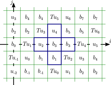
Figure 27: Face weights for the explicit solution of the short diagonal hyperplane map. The shown Aztec diamond corresponds to the computation of $T^{2}(u)_{3}$.

Theorem 10.3.

Consider the coordinates $(u_{i})_{i\in\mathbb{Z}}$ of a polygon and $(b_{i})_{i\in\mathbb{Z}}$ of a companion polygon. Let $v:\mathbb{Z}\rightarrow{\mathbb{R}\mathrm{P}}^{3}$ be a polygon and $c:\mathbb{Z}\rightarrow{\mathbb{R}\mathrm{P}}^{3}$ a companion polygon, and let $u,b$ be the affine coordinates of $v,c$, and $T$ be the short diagonal hyperplane map dynamics. Consider the graph $\mathbb{Z}^{2}$ with face-weights $(a_{i,j})_{(i,j)\in\mathbb{Z}^{2}}$ given by,

$$a_{i,j}=\begin{cases}b_{i+j-\lfloor\frac{i-j}{4}\rfloor}&\mbox{if }[i-j]_{4}=0,3\\ T(u)_{i+j-\lfloor\frac{i-j}{4}\rfloor}&\mbox{if }[i-j]_{4}=1,\\ u_{i+j-\lfloor\frac{i-j}{4}\rfloor}&\mbox{if }[i-j]_{4}=2.\end{cases}$$ (10.8)

Then, for all $(i,k)\in\mathbb{Z}^{2}$ such that $k\geq 1$ we have

$$T^{k}(u)_{i} =\begin{cases}Y\left(A_{2k-2}(\frac{i}{2}+k+2,\frac{i}{2}-k-1),a\right)&\text{if }[i]_{2}=0,\\ Y\left(A_{2k-2}(\frac{i-1}{2}+k,\frac{i-1}{2}-k+1),a\right)&\text{if }[i]_{2}=1.\end{cases}$$ (10.9)

Proof.

Consider the function $x:\mathcal{L}\rightarrow\hat{\mathbb{R}}$ given by

$$x(i,j,k)=\begin{cases}T^{\lfloor\frac{k}{2}\rfloor}(b)_{i+j-\lfloor\frac{i-j-k}{4}\rfloor}&\mbox{if }[i-j+k]_{4}=0,\\ T^{\lfloor\frac{k+1}{2}\rfloor}(u)_{i+j-\lfloor\frac{i-j-k}{4}\rfloor}&\mbox{if }[i-j+k]_{4}=2.\par\end{cases}$$ (10.10)

This is a solution to the dSKP recurrence. Indeed, the relation

$$\frac{(x_{-e_{3}}-x_{e_{2}})(x_{-e_{1}}-x_{e_{3}})(x_{-e_{2}}-x_{e_{1}})}{(x_{e_{2}}-x_{-e_{1}})(x_{e_{3}}-x_{-e_{2}})(x_{e_{1}}-x_{-e_{3}})}=-1,$$ (10.11)

at $p\in\mathbb{Z}^{3}\setminus\mathcal{L}$ can be checked with some case handling. For instance, if $p=(i,j,k)$ with $[i-j+k]_{4}=1$ and $[k]_{2}=1$, one can check that $x_{-e_{3}}(p)=x_{-e_{1}}(p)$ while $x_{e_{1}}(p)=x_{e_{3}}(p)$, from which (10.11) is trivial. If $[i-j+k]_{4}=1$ and $[k]_{2}=0$, then for some $n,\ell\in\mathbb{Z}$, we have

$$x_{-e_{3}}(p)=T^{\ell}(b)_{n}, x_{e_{2}}(p)=T^{\ell+1}(b)_{n+1}, x_{-e_{1}}(p)=T^{\ell+1}(b)_{n-1},$$

$$x_{e_{3}}(p)=T^{\ell+2}(u)_{n}, x_{-e_{2}}(p)=T^{\ell+1}(u)_{n-1}, x_{e_{1}}(p)=T^{\ell+1}(u)_{n+1},$$

and (10.11) is an application of the second relation of Lemma 10.2. Similarly for $[i-j+k]_{4}=3$, when $[k]_{2}=0$ the relation is trivial, while for $[k]_{2}=1$ it is an application of the first relation of Lemma 10.2.

It is direct to check that the function $x$ satisfies the initial condition $a_{i,j}=x(i,j,[i+j]_{2})$ of the theorem, and that for $i$ even, $T^{k}(u)_{i}=x\left(\frac{i}{2}+k+2,\frac{i}{2}-k-1,2k-1\right)$ while for $i$ odd, $T^{k}(u)_{i}=x\left(\frac{i-1}{2}+k,\frac{i-1}{2}-k-1,2k-1\right)$. Using Theorem 2.2 yields the theorem. ∎

Next, we consider a conjecture of Glick [Gli15, Conjecture 9.2]. An $m$-periodic polygon is a polygon $(v_{i})_{i\in\mathbb{Z}}$ such that $v_{i+m}=v_{i}$ for all $i\in\mathbb{Z}$.

Theorem 10.4.

Let $v$ be an $2m$-periodic polygon and $P_{0},P_{1}\in{\mathbb{R}\mathrm{P}}^{3}$. Assume for all $i\in\mathbb{Z}$ that the plane $v_{i-1}v_{i}v_{i+1}$ contains $P_{[i]_{2}}$. If $T^{m-3}(v)$ exists, then there are two planes $E_{0},E_{1}\subset{\mathbb{R}\mathrm{P}}^{3}$ such that for all $i\in\mathbb{Z}$ the point $T^{m-3}(v)_{i}$ is contained in $E_{[i]_{2}}$.

Proof.

We first prove the theorem for $(v_{i})_{i\in\mathbb{Z}}$ a polygon in ${\mathbb{C}\mathrm{P}}^{3}$, with all the other objects defined on $\mathbb{C}$ as well. One can easily check that all the previous results in this section hold for complex points.

First, let us show that for any $2m$-periodic polygon there is a $2m$-periodic companion polygon. Let us denote by $\hat{v}_{i}$, $\hat{c}_{i}$ a homogeneous lift to $\mathbb{C}^{4}$ of $v_{i},c_{i}$ for any $i\in\mathbb{Z}$. Assume $\hat{c}_{i-2}$ is given. Then any lift $\hat{c}_{i}$ can be expressed as a function of $\hat{c}_{i-2}$: by definition, it has to be in span $\langle\hat{v}_{i-1},\hat{v}_{i+1}\rangle$ and in the span $\langle\hat{v}_{i-2},\hat{v}_{i},\hat{c}_{i-2}\rangle$, which gives the formula

$$\hat{c}_{i}=\det(\hat{v}_{i-2},\hat{c}_{i-2},\hat{v}_{i},\hat{v}_{i+1})\hat{v}_{i-1}-\det(\hat{v}_{i-2},\hat{c}_{i-2},\hat{v}_{i},\hat{v}_{i-1})\hat{v}_{i+1}.$$ (10.12)

By iterating, we can express $\hat{c}_{2m}$ as a linear function of $\hat{c}_{0}$. This linear function takes values in the span $\langle\hat{v}_{-1},\hat{v}_{1}\rangle$, so by taking $\hat{c}_{0}$ in this subspace, we get a linear transformation of this $2$-dimensional subspace. This transformation has at least one eigenvector (this is where we use the fact that the base field is $\mathbb{C}$), so taking $\hat{c}_{0}$ to be this eigenvector, we get that $\hat{c}_{2m}$ is proportional to $\hat{c}_{0}$, therefore $c_{2m}=c_{0}$. We may do the same to get that $c_{1}=c_{2m+1}$ as well in ${\mathbb{C}\mathrm{P}}^{3}$. This gives the desired $2m$-periodic companion polygon.

A consequence of Equation (10.1) is that

$$T^{-1}(v)_{i}=v_{i-3}v_{i-2}v_{i-1}\cap v_{i-1}v_{i}v_{i+1}\cap v_{i+1}v_{i+2}v_{i+3},$$ (10.13)

therefore $T^{-1}(v)_{i}=P_{[i]_{2}}$. Let $c$ be a companion polygon of $v$, and let $u,b$ be affine coordinates of $v,c$. $T^{-1}(u)$ is singular, so if $x$ is defined by Equation (10.10), we can define the new solution to dSKP by $y(i,j,k)=x(i,j,k-2)$ and check that $y$ is $(m,2)$-Devron. Applying Theorem 2.8 to $y$, we get that $T^{m-2}(b)$ takes only two values (one for even indices and one for odd indices). This being true for any affine coordinates of $v$ and $c$ implies that there are points $B_{0},B_{1}\in{\mathbb{C}\mathrm{P}}^{3}$ such that $T^{m-2}(c)_{i}=B_{[i]_{2}}$ for all $i\in\mathbb{Z}$. By definition of the companion polygon, each line $T^{m-2}(v)_{i-1}T^{m-2}(v)_{i+1}$ contains $B_{[i]_{2}}$. Therefore, there are two lines $L_{0},L_{1}\subset{\mathbb{C}\mathrm{P}}^{3}$ such that $T^{m-2}(v)_{i}\in L_{[i]_{2}}$ for all $i\in\mathbb{Z}$. Additionally, by Equation (10.1), $T^{m-2}(v)_{i}\in T^{m-3}(v)_{i-1}T^{m-3}(v)_{i+1}$. As a consequence, each plane $E_{i}=T^{m-3}(v)_{i-2}T^{m-3}(v)_{i}T^{m-3}(v)_{i+2}$ contains the two points $T^{m-2}(v)_{i-1}$ and $T^{m-2}(v)_{i+1}$ and therefore also the line $L_{[i+1]_{2}}$. This in turn implies that all the even $E_{i}$ coincide and that all the odd $E_{i}$ coincide, or that each plane $E_{i}$ is just a line, specifically the line $L_{[i+1]_{2}}$. In either case, the claim is proven, for points in ${\mathbb{C}\mathrm{P}}^{3}$.

Going back to the statement of the theorem, if points are defined over $\mathbb{R}$, then the previous reasoning applies and shows that there exist planes $E^{\prime}_{0},E^{\prime}_{1}$ in ${\mathbb{C}\mathrm{P}}^{3}$ such that for all $i\in\mathbb{Z}$, the point $T^{m-3}(v)_{i}$ is contained in $E^{\prime}_{[i]_{2}}$. So for instance the points $(T^{m-3}_{i})_{[i]_{2}=0}$ are coplanar in ${\mathbb{C}\mathrm{P}}^{3}$, but also have real coordinates, as the dynamics (10.1) preserves real coordinates. This implies that they are coplanar in ${\mathbb{R}\mathrm{P}}^{3}$. To see this, one can consider lifts of $(T^{m-3}_{i})_{[i]_{2}=0}$ in $\mathbb{R}^{4}$: these points belong to a common $3$-dimensional complex subspace, so there is a nonzero vector $v\in\mathbb{C}^{4}$ orthogonal to all of them, but then both $\mathrm{Re}(v)$ and $\mathrm{Im}(v)$ are orthogonal to all of them, and one of these has to be nonzero. Of course the same argument applies to $(T^{m-3}_{i})_{[i]_{2}=1}$.

∎

References

- [AB00] Sergey I. Agafonov and Alexander I. Bobenko. Discrete and Painlevé equations. International Mathematics Research Notices, 2000(4):165–193, 01 2000.
- [AB03] Sergey I. Agafonov and Alexander I. Bobenko. Hexagonal circle patterns with constant intersection angles and discrete Painlevé and Riccati equations. Journal of Mathematical Physics, 44(8):3455–3469, 2003.
- [ABS03] Vsevolod E. Adler, Alexander I. Bobenko, and Yuri B. Suris. Classification of integrable equations on quad-graphs. The consistency approach. Comm. Math. Phys., 233(3):513–543, 2003.
- [Adl93] Vsevolod E. Adler. Recuttings of polygons. Functional Analysis and Its Applications, 27(2):141–143, Apr 1993.
- [AdTM22] Niklas C. Affolter, Béatrice de Tilière, and Paul Melotti. The Schwarzian octahedron recurrence (dSKP equation) I: explicit solutions, 2022. Preprint on arXiv.
- [Aff21] Niklas C. Affolter. Miquel dynamics, Clifford lattices and the Dimer model. Letters in Mathematical Physics, 111:1–23, 2021.
- [Aff22] Niklas C. Affolter. Discrete Differential Geometry and Cluster Algebras via TCD maps, 2022. PhD thesis, in preparation.
- [BH03] Alexander I. Bobenko and Tim Hoffmann. Hexagonal circle patterns and integrable systems: Patterns with constant angles. Duke Mathematical Journal, 116(3):525 – 566, 2003.
- [BK98a] Leonid V. Bogdanov and Boris G. Konopelchenko. Analytic-bilinear approach to integrable hierarchies. I. Generalized KP hierarchy. Journal of Mathematical Physics, 39(9):4683–4700, 1998.
- [BK98b] Leonid V. Bogdanov and Boris G. Konopelchenko. Analytic-bilinear approach to integrable hierarchies. II. Multicomponent KP and 2D Toda lattice hierarchies. Journal of Mathematical Physics, 39(9):4701–4728, 1998.
- [BMS05] Alexander I. Bobenko, Christian Mercat, and Yuri B. Suris. Linear and nonlinear theories of discrete analytic functions. Integrable structure and isomonodromic Green’s function. Journal für die reine und angewandte Mathematik, 2005(583):117–161, 2005.
- [BP96] Alexander I. Bobenko and Ulrich Pinkall. Discrete isothermic surfaces. Journal für die reine und angewandte Mathematik, 1996(475):187–208, 1996.
- [BP99] Alexander I. Bobenko and Ulrich Pinkall. Discrete integrable geometry and physics, chapter Discretization of surfaces and integrable systems, page 3–58. Oxford University Press, 1999.
- [BS02] Alexander I. Bobenko and Yuri B. Suris. Integrable systems on quad-graphs. International Mathematics Research Notices, 2002(11):573–611, 01 2002.
- [BS08] Alexander I. Bobenko and Yuri B. Suris. Discrete Differential Geometry: Integrable Structure. Graduate studies in mathematics. Birkhäuser, 2008.
- [CLR20] Dmitry Chelkak, Benoît Laslier, and Marianna Russkikh. Dimer model and holomorphic functions on t-embeddings of planar graphs, 2020. Preprint, arXiv:2001.11871.
- [CLR21] Dmitry Chelkak, Benoît Laslier, and Marianna Russkikh. Bipartite dimer model: perfect t-embeddings and Lorentz-minimal surfaces, September 2021. Preprint, arXiv:2109.06272.
- [Cox89] Harold S. M. Coxeter. Introduction to Geometry. Wiley Classics Library. Wiley, 2 edition, 1989.
- [Duf56] Richard J. Duffin. Basic properties of discrete analytic functions. Duke Mathematical Journal, 23(2):335 – 363, 1956.
- [GK13] Alexander B. Goncharov and Richard W. Kenyon. Dimers and cluster integrable systems. Annales scientifiques de l’École Normale Supérieure, 46(5):747–813, 2013.
- [Gli11] Max Glick. The pentagram map and Y-patterns. Advances in Mathematics, 227(2):1019 – 1045, 2011.
- [Gli15] Max Glick. The Devron property. Journal of Geometry and Physics, 87:161–189, 2015.
- [Gli18] Max Glick. The Limit Point of the Pentagram Map. International Mathematics Research Notices, 2020(9):2818–2831, 05 2018.
- [GP16] Max Glick and Pavlo Pylyavskyy. Y-meshes and generalized pentagram maps. Proceedings of the London Mathematical Society, 112(4):753–797, 03 2016.
- [GRP91] Basil Grammaticos, Alfred Ramani, and Vassilios Papageorgiou. Do integrable mappings have the Painlevé property? Phys. Rev. Lett., 67:1825–1828, Sep 1991.
- [GSTV12] Michael Gekhtman, Michael Shapiro, Sergei Tabachnikov, and Alek Vainshtein. Higher pentagram maps, weighted directed networks, and cluster dynamics. Electronic Research Announcements, 19(0):1–17, 2012.
- [HV98] Jarmo Hietarinta and Claude Viallet. Singularity confinement and chaos in discrete systems. Phys. Rev. Lett., 81:325–328, Jul 1998.
- [Izo21] Anton Izosimov. Dimers, networks, and cluster integrable systems, 2021. Preprint, arXiv:2108.04975.
- [Izo22] Anton Izosimov. Polygon recutting as a cluster integrable system, 2022. Preprint, arXiv:2201.12503.
- [Kas61] Pieter W. Kasteleyn. The statistics of dimers on a lattice : I. The number of dimer arrangements on a quadratic lattice. Physica, 27:1209–1225, December 1961.
- [Kas67] Pieter W. Kasteleyn. Graph theory and crystal physics. In Graph Theory and Theoretical Physics, pages 43–110. Academic Press, London, 1967.
- [Ken02] Richard W. Kenyon. The Laplacian and Dirac operators on critical planar graphs. Inventiones mathematicae, 150(2):409–439, 2002.
- [KLRR18] Richard W. Kenyon, Wai Yeung Lam, Sanjay Ramassamy, and Marianna Russkikh. Dimers and Circle patterns, 10 2018. Preprint on arXiv:1810.05616.
- [KS02] Boris G. Konopelchenko and Wolfgang K. Schief. Menelaus’ theorem, Clifford configurations and inversive geometry of the Schwarzian KP hierarchy. Journal of Physics A: Mathematical and General, 35(29):6125–6144, 07 2002.
- [KS13] Boris Khesin and Fedor Soloviev. Integrability of higher pentagram maps. Mathematische Annalen, 357(3):1005–1047, Nov 2013.
- [Lam16] Wai Yeung Lam. Discrete Minimal Surfaces: Critical Points of the Area Functional from Integrable Systems. International Mathematics Research Notices, 2018(6):1808–1845, 12 2016.
- [Mar13] Gloria Marí Beffa. On Generalizations of the Pentagram Map: Discretizations of AGD Flows. Journal of Nonlinear Science, 23(2):303–334, Apr 2013.
- [Miq38] Auguste Miquel. Théorèmes sur les intersections des cercles et des sphères. J. Math. Pures Appl., pages 517–522, 1838.
- [Mü15] Christian Müller. Planar discrete isothermic nets of conical type. Beiträge zur Algebra und Geometrie / Contributions to Algebra and Geometry, 57, 06 2015.
- [NC95] Frank Nijhoff and Hans Capel. The discrete Korteweg-de Vries equation. Acta Applicandae Mathematica, 39(1):133–158, Jun 1995.
- [OST10] Valentin Ovsienko, Richard Schwartz, and Serge Tabachnikov. The Pentagram Map: A Discrete Integrable System. Communications in Mathematical Physics, 299(2):409–446, Oct 2010.
- [Ram18] Sanjay Ramassamy. Miquel Dynamics for Circle Patterns. International Mathematics Research Notices, 2020(3):813–852, 03 2018.
- [RG11] Jürgen Richter-Gebert. Perspectives on Projective Geometry: A Guided Tour Through Real and Complex Geometry. Springer Publishing Company, Incorporated, 1st edition, 2011.
- [Sch92] Richard Schwartz. The pentagram map. Experiment. Math., 1(1):71–81, 1992.
- [Sch97] Oded Schramm. Circle patterns with the combinatorics of the square grid. Duke Mathematical Journal, 86(2):347 – 389, 1997.
- [Sch07] Richard Schwartz. Discrete monodromy, pentagrams, and the method of condensation. Journal of Fixed Point Theory and Applications, 3:379–409, 2007.
- [Sch09] Wolfgang K. Schief. Discrete Laplace-Darboux sequences, Menelaus’ theorem and the pentagram map, 2009. Talk at workshop: Geometric Aspects of Discrete and Ultra-discrete Integrable Systems, Glasgow.
- [Smi10] Stanislav Smirnov. Discrete Complex Analysis and Probability, pages 595–621. 2010.
- [Sol11] Fedor Soloviev. Integrability of the pentagram map. Duke Mathematical Journal, 162, 06 2011.
- [Spe07] David E Speyer. Perfect matchings and the octahedron recurrence. Journal of Algebraic Combinatorics, 25(3):309–348, 2007.
- [Ste02] Kenneth Stephenson. Chapter 11 - Circle Packing and Discrete Analytic Function Theory. In R. Kühnau, editor, Geometric Function Theory, volume 1 of Handbook of Complex Analysis, pages 333–370. North-Holland, 2002.
- [TT13] Sergei Tabachnikov and Emmanuel Tsukerman. On the discrete bicycle transformation. In Proceedings of the Montevideo Dynamical Systems Congress 2012, volume 14 of Publicaciones Matemáticas del Uruguay, pages 201–220, 2013.
- [Vin93] Ėrnest B. Vinberg. Geometry II: Spaces of Constant Curvature. Encyclopaedia of mathematical sciences. Springer-Verlag, 1993.
- [Wei21] Max H. Weinreich. The Algebraic Dynamics of the Pentagram Map, 2021. Preprint, arXiv:2104.06211.
- [Yao14] Zijian Yao. Glick’s conjecture on the point of collapse of axis-aligned polygons under the pentagram maps, 2014. Preprint, arXiv:1410.7806.