Fast Convergence Time Synchronization in Wireless Sensor Networks Based on Average Consensus

Abstract

Average consensus theory is intensely popular for building time synchronization in wireless sensor network (WSN). However, the average consensus-based time synchronization algorithm is based on iteration that pose challenges for efficiency, as they entail high communication cost and long convergence time in large-scale WSN. Based on the suggestion that the greater the algebraic connectivity leads to the faster the convergence, a novel multi-hop average consensus time synchronization (MACTS) is developed with innovative implementation in this paper. By employing multi-hop communication model, it shows that virtual communication links among multi-hop nodes are generated and algebraic connectivity of network increases. Meanwhile, a multi-hop controller is developed to balance the convergence time, accuracy and communication complexity. Moreover, the accurate relative clock offset estimation is yielded by delay compensation. Implementing the MACTS based on the popular one-way broadcast model and taking multi-hop over short distances, we achieve hundreds of times the MACTS convergence rate compared to ATS.

I Introduction

Synchronization is an important part of the distributed system, e.g., synchronization control [TIE_2], synchronization measurement [TIE_8], internet of things [TS-IOT, TII_6]. For the wireless sensor networks (WSN), time synchronization is used to generate consistent time concept for data acquisition [TII_1, DataAqu, TII_2], intelligent sleeping [2], location services [3, Localtion_TII] and so on. Because of the extra hardware required or the complex protocols employing in the Network Time Protocol, Global Navigation Satellite System and IEEE 1588 Standard (Precision Time Protocol) may not meet the synchronization requirements in WSN applications.

In low-cost, low-power, energy-constrained, and large-scale WSN applications, the convergence rate is intensely important to an accurate, robust and energy-efficient time synchronization algorithm. A faster-convergence approach requires less synchronization intervals and message transmissions to obtain the expected synchronization accuracy, meanwhile, it may adapts quickly to the changes in network structure and clock drifts (e.g., due to variances in temperature or voltage).

Until now, numerous time synchronization algorithms have been proposed for WSN, and they can be simply summarized as centralized, semi-distributed, and fully distributed. The centralized time synchronization algorithms, e.g., the TPSN [TPSN], RBS [RBS], CESP [CESP], R-Sync [R-Sync], and cluster-based consensus time synchronization [cluster-Conse-sync-1, cluster-Conse-sync-2, cluster-Conse-sync-3, PulseSS], require additional topology management protocol (e.g., spanning tree protocol, and clustering protocol) to guarantee its validity. While, considering the large-scale WSN, the changes in the topology will cause the algorithms to fail. Thus, the centralized algorithms may well meet the time synchronization of lightweight static rather than large-scale dynamic WSN.

Both the semi-distributed and fully distributed time synchronization algorithms require none topology management protocol. The flooding time synchronization algorithms, e.g., FTSP [FTSP], EGSync [EGSync], Glossy [Glossy], PulseSync [PulseSync], FCSA [FCSA], PISync [PISync], and RMTS [RMTS], are the typical semi-distributed approach. The key idea is: a special node (i.e., reference) periodically broadcasts its time information, which is then flooded in network-wide, meanwhile other nodes try to synchronize themselves to the reference. While, in the fully distributed approaches, e.g., DCTS [DCTS], ATS [ATS], MTS [MTS], GTSP [GTSP], CCS [CCS], and DiStiNCT [DiStiNCT], none reference is required and each node synchronize to its neighbors, in other words, they use local information to achieve a global agreement. Therefore, the distributed approaches are more scalable and robust, and thus are paid more attention in the recent years.

The average consensus theory is widely used in many fields, e.g., distributed control [cons-control-1, cons-control-4], tracking [consensus-tracking], and smart grid [SmartGrid_EnergyMan]. Moreover, it is popular used to develop a fully distributed time synchronization protocol for a dynamic WSN, e.g., the ATS. The average consensus-based time synchronization algorithm is easily to implement, but is more robust and scalable in dynamic networks than most of other time synchronization protocols. However, it is difficult to predict the convergence time due to iteration, and needs to be improved in terms of convergence rate and synchronization accuracy.

Regarding synchronization convergence rate, as described in [ATS], in a $5\times 7$ grid network (diameter of 10), ATS converges after 120 rounds of synchronization intervals. As shown in the experimental results of this paper, e.g., a $5\times 5$ grid network (diameter of 8), the ATS requires approximately 24 rounds of synchronization intervals to convergent. While, considering the line network (diameter of 8), it requires about approximately 60 rounds of synchronization intervals. The maximum-consensus-based protocols MTS [MTS] converge faster than ATS, but they still cost approximately 90 rounds to converge in a 20-node ring network (diameter of 10), and their convergence time is linear growth of the diameter. However, considering the flooding time synchronization algorithm, the FTSP and PulseSync can converge with less than 20 rounds of synchronization intervals in a 31-node line network (diameter of 29) [FCSA], and the RMTS can converge after the 2-nd synchronization interval in a 25-node line network (diameter of 24) [RMTS].

In terms of synchronization accuracy, ATS uses one-way broadcast model to generate the relative clock offset estimation; that is, the timestamps that are created by the broadcast frame at the transmitting node and the receiving node, respectively, are used to calculate the relative clock offset estimation. Unfortunately, in which the message delay is directly introduced into the estimation. In one-way broadcast time synchronization, there is currently no better way to eliminate the synchronization error that caused by delay, but uses previous experimental test results to estimate the mean of delay and then compensate the relative clock offset estimation by the mean, just like PulseSync and RMTS.

It has got detailed proof in [14] that, the average consensus convergence rate equals to the algebraic connectivity of a strongly connected digraph. Moreover, the algebraic connectivity strongly depends on the structure and connections of the graph, and it is relatively large for dense graphs with more connections. Therefore, increasing the algebraic connectivity should be an efficient way to improve the convergence rate. In [Conv-Analysis-Consensus], it is recommended to increase the nearest neighbors or transmission radius without effecting the power consumption. While, considering the low-cost and energy-constrained WSN, it may be unreasonable due to the strong relationship between transmission distance and transmission power. In other words, physically changing the topology is difficult in WSN. The [15] developed an multi-hop relay protocol for multi-agent system to get an better convergence rate without changing topology, in which a large number of virtual connection are generated to the improve on algebraic connectivity. However, considering the large-scale WSN, the multi-hop communication may seriously increases the message and computation complexity [15]. Moreover, it may results in a by-hop error accumulation problem [RMTS].

In this paper, we focus on an accurate average consensus time synchronization algorithm that converges fast. The multiple-hop average consensus time synchronization (MACTS) algorithm is proposed based on multiple-hop one-way broadcast model, and the main important improvements of MACTS are as follows.

1) The convergence rate is greatly improved in MACTS. Multi-hop communication is used to generate virtual connection between multi-hop nodes, which may brings order of magnitude improvement in algebraic connectivity and convergence rate.

2) A multi-hop controller is developed to optimize drawbacks due to multi-hop communication in MACTS. To obtain a fast convergence, it employs a multi-hop communication at the initial phase of network; to simplify the message complexity and against the by-hop error accumulation, it adaptively switches to single-hop communication after the synchronization converges.

Moreover, a delay estimate is calculated from the results of previous experimental results, and it is used to compensate the relative clock offset estimation in MACTS.

The remainder of this paper is organized as follows. The system model is provided In Section II. We present and analyze the MACTS in Section III. The implementation of MACTS is developed in Section IV. The experimental results and simulation are presented and discussed in Section V and VI, respectively. Conclusions are given in Section VII.

II System Model

The WSN is modeled as the graph $\mathcal{G}=(\mathcal{N},\mathcal{E})$, where $\mathcal{N}=\{1,2,\ldots,\mathcal{N}\}$ represents the nodes of the WSN and $\mathcal{E}$ defines the available communication links. The set of neighbors for $v_{i}$ is $\mathcal{N}_{i}=\{j\mid(i,j)\in\mathcal{E},i\neq j\}$, where nodes $v_{i}$ and $v_{j}$ belong to $\mathcal{N}$, and $j\in\mathcal{N}_{i}$.

There are two time notions defined for the time synchronization algorithm, i.e. the hardware clock notion $H(t)$, and logical clock notion $L(t)$. The $H(t)$ is defined as

$$H(t)=\int_{0}^{t}h(\tau)d\tau+\theta(t_{0}),$$ (1)

where $h(\tau)$ is the hardware frequency rate (clock speed) of the clock source. The $h(\tau)$ is the inherent attribute of crystal oscillator; it cannot be changed or measured. Any node considers itself having the ideal clock frequency (i.e., nominal frequency), and $h(\tau)=1$. The variable $t_{0}$ is the moment that node is powered on and $\theta(t_{0})$ the initial relative clock offset. It should be noted that $H(t)$ cannot be changed also, and the timestamps on $H(t)$ are used to estimate the relative clock speed for the proposed algorithm.

The $L(t)$ is defined as

$$L(t)=\varphi(t)\times H(t),$$ (2)

where $\varphi(t)$ is the logical relative clock rate and initialized as 1; it can be changed to speed up or slow down $L(t)$. With respect to the reference node, $\varphi(t)$ is always set as 1. The timestamps on $L(t)$ are used to estimate the relative clock offset for the proposed algorithm. $L(t)$ is used to supply the global time service for the synchronization applications in WSN.

Considering the arbitrary nodes $v_{i}$ and $v_{j}$, $L_{i}(t)$ and $L_{j}(t)$ are the logical times, respectively, and $\varphi_{i}^{j}$ is the relative frequency rate, which is

$$\varphi_{i}^{j}=\frac{H_{j}(t_{2})-H_{j}(t_{1})}{H_{i}(t_{2})-H_{i}(t_{1})},$$ (3)

where, in consideration of arbitrary moments $t_{1}<t_{2}$.

III The Proposed MACTS

III-A The MACTS Protocol

The key idea of the proposed MACTS is to increase the connection $\mathcal{E}$ by Building virtual communication links among multi-hop nodes, then increases the algebraic connectivity indirectly. While the added virtual connections dose not change the topology structure.

In MACTS, every node asynchronously and periodically broadcasts time synchronization messages to neighbor nodes. Considering a $5\times 5$ grid networks, taking 2-hop MACTS as an example, it is shown in Fig. 1. The solid arrows in the figure are 1-hop MACTS and the dotted lines show the 2-hops MACTS. The broadcast information of node $v_{R}$ is received and processed by its neighbor nodes (black nodes).

In mult-hops MACTS, neighbor nodes immediately forward the time information they received, as shown by the dotted arrows in the Fig. 1. At this time, the synchronous broadcast message of $v_{R}$ is not only processed by its neighbor nodes, but also by the 2-hop nodes (blue nodes). MACTS builds virtual connections between node $v_{R}$ and 2-hop nodes to increase the number of network connections. Here, parameter $H$ is defined as the multi-hop number.

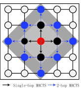
Figure 1: The 2-hop MACTS indication ($H=2$). Considering the moment that $v_{R}$ broadcast a packet, its neighbor will forward the received packet to the multi-hop node.

Figure 2 shows the implementation of multi-hop communication in MACTS. When the synchronization cycle of $v_{R}$ is triggered, its broadcast time message frame, i.e., $MSG_{1}$, will generate time stamps $T_{R,1}$ and $T_{j,1}$ in $v_{R}$ and $v_{j}$, respectively. In multi-hop MACTS, $v_{j}$ will forward the $MSG_{1}$ as soon as possible, i.e., the latency time $T_{d}\rightarrow 0$, then $MSG_{1,2}$ is forwarded to $v_{i}$. Thus, there is a virtual communication link is generated between $v_{R}$ and $v_{i}$.

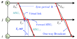
Figure 2: The 2-hop MACTS synchronization model. The 1-hop node forwards the packet as soon as possible, i.e., $T_{d}\rightarrow 0$.

The time information of the broadcast node is forwarded to the multiple-hop nodes by adjacent nodes, since there is many virtual communication links between broadcast and multiple-hop nodes; and the algebraic connectivity will be increased greatly.

1) Relative clock skew estimation: as shown in Fig. 2, according (3), the relative frequency rate estimation $\hat{\varphi}_{R}^{j}$ is given by

$$\hat{\varphi}_{j}^{R}=\frac{T_{j,2}-T_{j,1}}{T_{R,2}-T_{R,1}},$$ (4)

where the timestamps are created by the hardware clock $H(t)$.

2) Relative clock offset estimation: the clock offset estimation $\hat{\theta_{j}^{R}}$ is usually given by $\hat{\theta_{j}^{R}}=T_{j,1}-T_{R,1}$, where $T_{j,1}-T_{R,1}=\theta_{j}^{R}+D$. Variable $D$ is defined as the difference of a pair of time stamps, and the $D$ is comprised of the fixed portion $D_{fixed}$ and the variable portion $d$ [12, 13], i.e., $D=D_{fixed}+d$. In our experimental results, $\bar{D}$ is about 3.33 µs, $\sigma$ is 0.07, and $D$ is the normal distribution with 99.99% confidence determined by a t-test. Setting the fixed portion delay estimation $\hat{D}_{fixed}=\bar{D}$, then the $\hat{\theta_{j}^{R}}$ is

$$\hat{\theta}_{j}^{R}=T_{j,1}-T_{R,1}-\bar{D}=\theta_{R}^{j}+(D-\hat{D}_{fixed}),$$ (5)

where the timestamps are created by the logical clock $L(t)$. It can be seen that the estimation error of $\hat{\theta}_{R}^{j}$ is about $d$. Therefore, after $\hat{\varphi}_{j}^{R}$ converges, the MACTS can obtain a higher-precision relative clock offset estimation.

3) Synchronization error analysis: Base on the clock skew estimation and clock offset estimation, the local synchronization error in MACTS is given by

$$e_{l}(t)=(D-\hat{D}_{fixed})+({\varphi}_{j}^{R}-\hat{\varphi}_{j}^{R})\times t,$$ (6)

where, $t$ is the time after latest synchronization, i.e., $0<t<B$.

According the analysis in [RMTS], the by-hop error accumulation in the $k$-hop MACTS is given by

$$e_{m}[k]=\sum_{h=0}^{k-1}(D[h]-\hat{D}_{fixed})+\frac{\sum_{h=0}^{k-1}{(|a[h]-\hat{a}[h]|\times T_{d})}}{10^{6}},$$ (7)

where, $T_{d}\rightarrow 0$ is the waiting time of multi-hop node forward the time information.

III-B Averaging Problem and Convergence

1) Average-consensus: in [11, 14], the averaging problem is discussed in detail. Defining $x_{i}(0)$ as the initial state of node $i\in V$ and the state vector $x(t)=\{x_{1}(t),x_{2}(t),\ldots,x_{n}(t)\}$ of the node at time $k$, a consensus algorithm to update the state through the dynamic equation $x(t)$ is given as follow

$$x(t+1)=A(t)x(t).$$ (8)

The definition of matrix $A(t)$ is a non-negative matrix composed of $a_{ij}(t)$, which is a weighted adjacency matrix of $G$, and has $\sum_{j=1}^{n}a_{ij}(t)=1,(n\leq\mathcal{N})$ for any $v_{i}$; that is, $A(t)$ is a stochastic matrix. Then, the dynamic equation of the discrete consensus principle of any node i of the WSN is as follows [14]

$$x_{i}(k+1)=x_{i}(k)+\sum_{j\in\mathcal{N}_{i}}a_{ij}(k)(x_{j}(k)-x_{i}(k)).$$ (9)

For the static WSN $\mathcal{G}$, the set of its connection, $\mathcal{E}$, is a fixed value, and then the adjacency matrix is a fixed value; that is, $A(t)=A$. From [11], $\lim\limits_{{t\rightarrow\infty}}x_{i}(t)=\sum_{i=1}^{n}\pi_{i}x_{i}(0)$, where $\pi_{i}$ is the steady-state probability of the $v_{i}$ in the Markov chain associated with the stochastic matrix $A$. Then, if and only if any $v_{i}$ has $\pi_{i}=1/n$, the average consensus convergence is obtained. Therefore, using a doubly stochastic matrix, all nodes $v_{i}$ can converge to

$$\lim_{t\rightarrow\infty}x_{i}(t)=\frac{1}{n}\sum_{i=1}^{n}x_{i}(0),$$ (10)

where every node converges to the average of the initial state of all nodes. Specific proofs can be seen in [11, 14].

2) Algebraic connectivity and convergence rate: The convergence rate and convergence time of the average consensus algorithm directly depend on the algebraic connectivity of the $\mathcal{G}$. That is [14],

Lemma III.1

The more network connections and the greater the algebraic connectivity, the faster the convergence rate.

It defines that, a network with a fixed topology that is a strongly connected digraph, the globally asymptotically vanishes with a speed equal to the algebraic connectivity. The algebraic connectivity is determined by the topology and the edges of graphs, and it is relatively large for dense graphs (more edges), and is relatively small for sparse graphs (less edges) [14].

Considering node $v_{i}$ in $\mathcal{G}$, its size of neighbors is $|\mathcal{N}_{i}|$, and the in-degree and out-degree of node $v_{i}$ are

$$deg_{in}(v_{i})=\sum_{j=1}^{n}a_{ji},deg_{out}(v_{i})=\sum_{j=1}^{n}a_{ij}.$$ (11)

Because $\mathcal{G}$ is symmetrically connected, there are node connections that are bidirectional; that is, both the in-degree and the out-degree are equal to $|\mathcal{N}_{i}|$. The degree matrix $\mathcal{D}$ is a diagonal matrix. Then the Laplacian matrix $\mathcal{L}$ of the $\mathcal{G}$ is composed of the $A$ and $D$ of $\mathcal{G}$; that is

$$\mathcal{L}=\mathcal{D}-A.$$ (12)

The graph $\mathcal{G}$ has a weighted adjacency matrix $a_{ij}=a_{ij}\cdot w_{ij}$, where $w_{ij}>0$ is the associated weight of the pair of nodes $(i,j)$. The sum of arbitrary rows of the Laplacian matrix $\mathcal{L}$ is 0, and is a semi-positive definite matrix with $n$ non-negative eigenvalues $0=\lambda_{1}\leq\lambda_{2}\leq\ldots\leq\lambda_{n}$, where the second-smallest eigenvalue $\lambda_{2}$ is the algebraic connectivity of $\mathcal{G}$.

According to [15], for the symmetric directed graph $\mathcal{G}$, $\lambda_{2}$ can obtain the maximum value when all weights are the same; that is,

$$\lambda_{2}\leq\sum_{i\neq j}w_{ij}/(n-1).$$ (13)

Thus, when the directed graph $\mathcal{G}$ is set to the same weight $w_{ij}$, the average consensus protocol can obtain the maximum convergence rate. In the MACTS $w_{ij}$ is set to the constant 1.

According [14, 15], the algebraic connectivity $\lambda_{2}$ is determined by the topology structure of $\mathcal{G}$ and the connection $\mathcal{E}$, moreover, the $\lambda_{2}$ of a dense graph is relatively lager than that of a sparse graph.

III-C The Convergence Rate Analysis

The [Conv-Analysis-Consensus] suggests that, the number of neighbors and connections could be increased by increasing transmit power. However, in a static wireless sensor network, the network topology is fixed, and the transmit power (distance) of node is limited. In a dynamic wireless sensor network, the network topology dynamically changes randomly, and it cannot change according to the trend that is beneficial to increase the algebraic connectivity. Therefore, changing network topology is not the best choice to improve the convergence rate and does not meet the actual applications requirements.

In the proposed MACTS, the status information of the broadcast node is received not only by its neighbor nodes, but also by the multi-hop node. These multi-hop nodes constitutes virtual connection $\mathcal{E}$. It can be derived that the multi-hop consensus dynamic equation is [15]

$$x_{i}(k+1)=x_{i}(k)+ \sum_{j\in\mathcal{N}_{i}}a_{ij}(k)(x_{j}(k)-x_{i}(k)+$$ (14)

$$\sum_{s\in\mathcal{N}_{j}}a_{js}(k)(x_{s}(k)-x_{j}(k)+\ldots)).$$

For the directed graph $\mathcal{G}$, the directed graph is $\mathcal{G}_{1}$ when $H=1$, the directed graph is $\mathcal{G}_{2}$ when $H=2$, the directed graph is $\mathcal{G}_{3}$ when $H=3$, and so on. It can be seen from the above dynamic equations that the start and end points are links of the same node, which is a self-loop, and do not contribute to convergence, so these links are ignored in the subsequent discussion. In a multi-hop graph, there may be multiple H-hop links for pair of points, which are treated as paths here, and its weight is the sum of weights of all $H$-hop links. The algebraic connectivity of $\mathcal{G}_{1}$ is $\lambda_{2}(1)$.

Therefore, the adjacency matrix $A_{2}$ of $\mathcal{G}_{2}$ is [15]

$$a_{is}=\left\{\begin{aligned} &\sum_{j\in N_{i}}a_{ij}a_{js},(v_{i},v_{s})\in\mathcal{G}_{2}\\ &0\end{aligned}\right.$$ (15)

The corresponding Laplacian matrix is $\mathcal{L}_{2}$, the degree matrix is $D_{2}$, and the corresponding algebraic connectivity is $\lambda_{2}(2)$.

Similarly, the adjacency matrix $A_{3}$ of $\mathcal{G}_{3}$ is

$$a_{iz}=\left\{\begin{aligned} &\sum_{j\in N_{j}}a_{ij}(\sum_{s\in N_{j}}a_{js}a_{zs}),(v_{i},v_{z})\in\mathcal{G}_{3}\\ &0\end{aligned}\right.$$ (16)

The corresponding Laplacian matrix is $\mathcal{L}_{3}$, the degree matrix is $D_{3}$, and the corresponding algebraic connectivity of $\mathcal{G}_{H}$ is $\lambda_{2}(H)$.

Let the column vector $x$ of the matrix $W$ satisfy $xx^{T}=1$, and the sum of $x$ is 0. Based on the Courant-Fischer theorem, the second-smallest eigenvalue $\lambda_{2}$ of Laplacian matrix $\mathcal{L}$ is given by the following equation

$$\lambda_{2}=\min\limits_{x\in W}x^{T}Lx.$$ (17)

It is concluded that if $\mathcal{G}_{1}$ and $\mathcal{G}_{2}$ have the same vertex, $\mathcal{G}=\mathcal{G}_{1}\cup\mathcal{G}_{2}$, and $a(\mathcal{G})$ is the solution of the eigenvalue $\lambda_{2}$; then [15],

$$a(\mathcal{G}_{1})+a(\mathcal{G}_{2})\leq a(\mathcal{G}_{1}\cup\mathcal{G}_{2}).$$ (18)

The above conclusions can be generalized: If {$\mathcal{G}_{1}$,$\mathcal{G}_{2}$,$\ldots$,$\mathcal{G}_{H}$} satisfy the above conditions, then

$$a(\mathcal{G}_{1})+a(\mathcal{G}_{2})+\ldots+a(\mathcal{G}_{H})\leq a(\mathcal{G}_{1}\cup\mathcal{G}_{2}\cup\ldots\cup\mathcal{G}_{H}).$$ (19)

The similar conclusions are proved in [15].

Therefore, the algebraic connectivity $\lambda_{2}$ of the H-hop consensus described above satisfies the following formula

$$\lambda_{2}\geq\lambda_{2}(1)+\lambda_{2}(2)+\ldots\lambda_{2}(H).$$ (20)

As the hop $H$ increases, the algebraic connectivity $\lambda_{2}$ of $\mathcal{G}$ gradually increases, thereby improving the convergence rate of the consensus time synchronization.

IV Implementation

IV-A The Multi-hop MACTS

The pseudo-code of the MACTS is presented in Algorithm 1. Node $v_{i}$ is synchronized to the $v_{j}$ by calibrating $L_{i}(t)$ based on the rate multiplier $\varphi_{i}$ and clock offset estimation $\hat{\theta}_{i}^{j}$, where $v_{j}$ is the neighbor of $v_{i}$.

The multi-hop communication: node $v_{i}$ is broadcast periodically (period of $B$) to distribute the time information packets to neighbors, as in Algorithm 1, Line IV-A. Once the broadcast task is triggered, $v_{i}$ rapidly broadcasts a packet, as in Algorithm 1, Lines LABEL:alg1.4 and LABEL:alg1.5. Two group of timestamps are created over the phase of broadcasting, i.e., timestamp $H_{i}[n]$ (created on $H_{i}(t)$) and timestamp $L_{i}[n]$ (created on $L_{i}(t)$). The basic information of the broadcast packets comprise four parts: $H_{i}[n]$, $L_{i}[n]$, $\varphi_{i}$, and $ID_{scr}$ (Algorithm 1, Line LABEL:alg1.5). The $ID_{scr}$ is used to count the forward distance (hop) of the time information, and if $ID_{scr}$ achieves to the $H$, then the current multi-hop communication will be stopped, as in Algorithm 1, Lines LABEL:alg1.14, LABEL:alg1.12 and LABEL:alg1.13 .

1 Initialization:

2  Set $\varphi_{i}=1$, $\hat{\varphi}_{i}^{j}=1$, $\hat{\theta}_{i}^{j}=0$, $H=2$

3  Set $H_{i,old}=0$, $H_{j,old}=0$

4  Start periodic broadcast task, period of $B$

Algorithm 1 Algorithm pseudo-code for MACTS (taking 2 hops MACTS as an example, i.e., $H=2$ ), where $v_{j}\in N_{i}$.