DRSOM: A Dimension Reduced Second-Order Method

Abstract

In this paper, we propose a Dimension-Reduced Second-Order Method (DRSOM) for convex and nonconvex (unconstrained) optimization. Under a trust-region-like framework, our method preserves the convergence of the second-order method while using only curvature information in a few directions. Consequently, the computational overhead of our method remains comparable to the first-order such as the gradient descent method. Theoretically, we show that the method has a local quadratic convergence and a global convergence rate of $O(\epsilon^{-3/2})$ to satisfy the first-order and second-order conditions if the subspace satisfies a commonly adopted approximated Hessian assumption. We further show that this assumption can be removed if we perform a corrector step using a Krylov-like method periodically at the end stage of the algorithm. The applicability and performance of DRSOM are exhibited by various computational experiments, including $\mathcal{L}_{2}-\mathcal{L}_{p}$ minimization, CUTEst problems, and sensor network localization.

90C26, 90C30, 90C60, 65K05, 49M05, 49M37, 68Q25

1 Introduction

In this paper, we consider the following unconstrained optimization problem

(1) $$\min_{x\in\mathbb{R}^{n}}f(x),$$

where $f:\mathbb{R}^{n}\to\mathbb{R}$ is twice differentiable and possibly nonconvex and $f_{\inf}:=\inf f(x)>-\infty$. We aim to find a “stationary point” $x$ such that

(2) $$\|\nabla f(x)\|\leq\epsilon$$

and $x$ approximately satisfies the second-order necessary conditions in a certain subspace. Historically speaking, various methods have been proposed to solve (1), among which the first-order methods (FOM) based on the gradient of $f$ are the most popular ones. A first-order method computes a descent direction that iteratively decreases the function value, in which the negative gradient, the momentum [34] can be applied as to construct the iterates. Theoretically, FOMs has the global complexity rate in $O(\epsilon^{-2})$ [28], however, they only converge to a point that satisfies the first-order condition (2).

To escape the first-order saddle point, people may resort to the second-order methods based on the Hessian of $f$ with variants of Newton-type iterations. Traditionally, the global convergence of second-order method can be ensured by frameworks like line search and trust-region methods [30]. While these classical methods are efficient in practice due to local superlinear convergence rate, the global iteration complexity of the standard Newton’s method is generally in the same order as that of the gradient descent method [6]. To clear the mist, Nesterov and Polyak [29] established the first $O(\epsilon^{-3/2})$ iteration complexity for second-order methods using cubic-regularized Newton method (also see Cartis et al. [7, 8]). However, the complexity analysis for the trust-region methods seems to be more challenging. Ye [44] in his early lecture notes showed that the trust-region method with a fixed-radius strategy also has the iteration complexity of $O(\epsilon^{-3/2})$, which matches the iteration bound of the aforementioned cubic regularized Newton method. A more practical adaptive trust-region method with $O(\epsilon^{-3/2})$ bound was only unveiled in [15] until very recently.

When the problem dimension gets larger, both explicitly computing the Hessian matrix and solving Newton-type subproblems could be more costly. A practical implementation of the second-order method usually uses a Lanczos method to iteratively find inexact solutions [12, 8, 16], where the “inexactness” can be controlled by the quality of Hessian approximation in some sense [18, 7, 15, 40]. However, even this approach can be impractical for huge-sized problems, e.g., solving sensor-network localization for thousands of sensors that may induce a undirected graph with millions of edges. By contrast, the first-order methods that only require gradient and cheap directions are scalable well to those huge-sized problems. However, their numerical performance heavily relies on proper step sizes and other hyperparameters, e.g., using various line search methods [23], and adaptive strategies [24] in stochastic settings. The choice of step size itself requires plentiful experiment and trial procedure. Despite all these difficulties, these methods are prevalent in large scale optimization.

Our approach in this paper is motivated from finding stepsizes for adaptive gradient methods using the Polyak’s momentum [44]. Specifically, we introduce a Dimension-Reduced Second-Order Method (DRSOM) to construct and solve a low-dimensional quadratic model to select the stepsizes. The extra overhead of DRSOM is mostly due to constructing and solving such quadratic subproblems.

1.1 Related Work

DRSOM adopts the basic idea of manipulating the low-dimensional subspace. In optimization, the subspace method is fundamental and widely studied. For example, the gradient method can be seen as performing a one-dimensional subspace minimization. In trust-region literature, such a minimizer in $\mathcal{L}_{k}=\mathsf{span}\{g_{k}\}$ is referred to as the Cauchy point [12]. In comparison, Yuan and Stoer [45] discussed the quadratic approximation over different simple and specific subspaces with an emphasis on their close relationship to the (nonlinear) conjugate gradient method. The authors also provided convergence proofs for the cases based on exact and inexact linear searches. A notable extension of the idea in [45] was made in [37] to the trust-region methods. Briefly speaking, if the subspace is constructed from the previous gradients under the quasi-Newton framework, then one can show that the subspace minimization generates exactly the same iterates of a full-dimensional quasi-Newton algorithm (see [37, Lemma 2.3]). A comprehensive summary on subspace methods can be found in [46, 26].

In contrast with the deterministic setting mentioned above, the sketching techniques can also be seen as a stochastic subspace method. Early results of sketching appear in solving least-square problems and more generally in numerical linear algebra [39]. The basic idea is to replace the full Hessian with its approximation —without destroying the convergence. Using different sketching schemes on the Hessian matrix, Pilanci and Wainwright [33] discussed the convergence rates of the Newton method. This idea later became popular in stochastic second-order optimization [25, 2, 26], and in natural gradient method [41, 42] for training deep neural networks. In essence, since the sketching methods use random matrices, the convergence and complexity analyses are typically probabilistic or as expectation in some error metrics. Moreover, the assumptions required by sketching methods, once again, are usually expressed in expectations or probabilistic. In a high-level view, the random sketch matrix has many notable advantages, for example, it may help the algorithm to escape from saddle points efficiently in nonconvex optimization. In comparison, DRSOM is greedier and straightforward since the subspace is kept at a minimum behavior and only increased when using the corrector steps.

As for the momentum-based gradient method, its global convergence rate was only established for convex optimization problems, in terms of the average iterates [20] as well as the last iterate [36]. When the objective function is nonconvex, the sequence generated by the heavy ball method converges to a first-order stationary point [48, 31]. Later, Sun et al. [35] proved that heavy ball method could even escape saddle point. However, the complexity rates are generally not superior to the gradient method under the nonconvex setting . A recent work in [1] studied the convergence of heavy ball method under the Polyak–Łojasiewicz condition based on an analysis of the dynamic system.

An earlier line of modified first-order methods in the nonconvex case explored the idea of using second-order information in the Nesterov’s accelerated gradient method (AGD), where the momentum direction is also appeared. For example, Carmon et al. [5, 4] used the negative curvature with AGD to achieve a better complexity bound of $O(\epsilon^{-7/4}\log(\epsilon^{-1}))$ for first-order methods. In this vein of research, the improved bound is based on finding the negative curvature with less dimension-dependent complexity. With the help of negative curvature, these methods are able to “escape” from saddle points efficiently and converge to the approximate second-order points in sharp comparison to classical first-order methods.

1.2 Our Contribution

In light of the above discussion, this paper extends previous results by demonstrating that one may efficiently enjoy the charisma of second-order information while keeping the low per-iteration cost of a first-order method.

• Firstly, we introduce a general dimension-reduced framework DRSOM by solving cheap subproblems without invoking the full Hessian matrix, see algorithm 1. We further propose some efficient constructions of the low dimensional subproblems based on Hessian-vector products or interpolation. Notably, the DRSOM can be viewed from the subspace perspective [45, 47, 26], however the associated analysis of global and local rates of convergence is missing. To our best knowledge, the interpolation technique is rarely celebrated in subspace and dimension reduction literature.

• Secondly, we analyze the convergence of DRSOM based on the discussion in [44]. Under a commonly adopted approximated Hessian assumption (cf. [7, AM.4]), we show that DRSOM has a local quadratic convergence and has an $O(\epsilon^{-3/2})$ complexity to globally converge to a point satisfying the first-order condition (2) and the second-order condition in a certain subspace. We identify that this assumption is only needed at the end stage of the algorithm and can be further removed if we periodically perform a corrector step, which is a Krylov-like method.

• Finally, we perform comprehensive experiments on nonconvex problems. Our results demonstrate its comparable performance to SOMs (e.g. the Newton trust-region method) in terms of the iteration number and to FOMs (e.g., conjugate gradient method) in terms of the per-iteration cost. We highlight a set of results in sensor network localization problem, from which we see DRSOM has the better performance in comparison to a well-known nonlinear conjugate gradient method.

Our paper is organized as follows. In Section 2, we discuss the details of the DRSOM including its important building blocks. Section 3 is regarding the convergence results of DRSOM such as the global convergence rate and local convergence rate. Finally, the comprehensive numerical results of DRSOM are presented in Section 4.

2 The DRSOM

2.1 Notations and Assumptions

We first introduce a few notations and technical lemmas. We denote the standard Euclidean norm by $\|\cdot\|$. If $A\in\mathbb{R}^{n\times n}$, then $\|A\|$ is the induced $\mathcal{L}_{2}$ norm and $A\succeq 0$ indicates that $A$ is positive semidefinite. To facilitate discussion, we denote $g_{k}=g\left(x_{k}\right)=\nabla f\left(x_{k}\right),H_{k}=$ $H\left(x_{k}\right)=\nabla^{2}f\left(x_{k}\right)$, and $d_{k}=x_{k}-x_{k-1}$ throughout the paper. We use $\mathcal{N}\left(\mu,\sigma^{2}\right)$ to denote the normal distribution with mean $\mu$, and variance $\sigma^{2}$.

In the rest of the paper, we assume $f$ is bounded below and is twice differentiable with $L$-Lipschitz gradient and $M$-Lipschitz Hessian, which is the standard assumption for second-order methods.

Assumption 1.

$f$ has $L$-Lipschitz continuous gradient and $M$-Lipschitz continuous Hessian, i.e., for $\forall x,y\in\mathbb{R}^{n}$,

(3) $$\|\nabla f(x)-\nabla f(y)\|\leq L\|x-y\|\quad\mbox{and}\quad\|\nabla^{2}f(x)-\nabla^{2}f(y)\|\leq M\|x-y\|.$$

The results in the following lemma are also standard and implied by the first- and second-order Lipshitz continuity.

Lemma 1 (Nesterov [28]).

If $f:\mathbb{R}^{n}\mapsto\mathbb{R}$ satisfies the Assumption 1, then, for all $x,y\in\mathbb{R}^{n}$,

(4a) $$|f(y)-f(x)-\nabla f(x)^{T}(y-x)\leq\frac{L}{2}\|y-x\|^{2}$$

(4b) $$\left\|\nabla f(y)-\nabla f(x)-\nabla^{2}f(x)(y-x)\right\|\leq\frac{M}{2}\|y-x\|^{2}$$

(4c) $$\left|f(y)-f(x)-\nabla f(x)^{T}(y-x)-\frac{1}{2}(y-x)^{T}\nabla^{2}f(x)(y-x)\right|\leq\frac{M}{6}\|y-x\|^{3}$$

We will use the results above repetitively throughout the analysis of the paper.

2.2 Overview of the Algorithm

We now give a brief overview of our method. In each iteration of the Dimension-Reduced Second-Order Method (DRSOM), we update

$$x_{k+1}=x_{k}-\alpha_{k}^{1}g_{k}+\alpha_{k}^{2}d_{k},$$

and the step size $\alpha_{k}=(\alpha_{k}^{1},\alpha_{k}^{2})$ is determined by solving the following 2-dimensional quadratic model $m_{k}(\alpha)$ :

(5) $$\min_{\alpha\in\mathbb{R}^{2}} ~{}m_{k}(\alpha):=f(x_{k})+(c_{k})^{T}\alpha+\frac{1}{2}\alpha^{T}Q_{k}\alpha$$

$$~{}\mathrm{s.t.}{}{} \|\alpha\|_{G_{k}}:=\sqrt{\alpha^{T}G_{k}\alpha}\leq\Delta,\quad\mbox{with}\quad G_{k}=\left[\begin{array}[]{cc}\left(g_{k}\right)^{T}g_{k}&-\left(g_{k}\right)^{T}d_{k}\\ -\left(g_{k}\right)^{T}d_{k}&\left(d_{k}\right)^{T}d_{k}\end{array}\right],\;$$

where

$$Q_{k}=\begin{bmatrix}(g_{k})^{T}H_{k}g_{k}&-(d_{k})^{T}H_{k}g_{k}\\ -(d_{k})^{T}H_{k}g_{k}&(d_{k})^{T}H_{k}d_{k}\end{bmatrix}\in\mathcal{S}^{2},\;c_{k}=\begin{bmatrix}-\left\|g_{k}\right\|^{2}\\ (g_{k})^{T}d_{k}\end{bmatrix}\in\mathbb{R}^{2}.$$

The idea of minizing a low-dimensional quadratic model in the objective was previously studied in Ye [44], Yuan and Stoer [45]. The novel ingredient in this paper is to impose a $2\times 2$ trust-region step to determine the step-sizes, which is necessary for solving nonconvex problems. In particular, the trust-region framework is adopted to ensure the global convergence by controling the progress made at each step. Similar to the standard trust-region method, after computing a trial step $d_{k+1}$, we introduce the reduction ratio $\rho_{k}$ for $m_{k}$ at iterate $x_{k}$,

$$\rho_{k}:=\frac{f\left(x_{k}\right)-f\left(x_{k}+d_{k+1}\right)}{m_{k}(0)-m_{k}\left(\alpha_{k}\right)},$$

if $\rho_{k}$ is too small, especially when $\rho_{k}<0$, it means our quadratic model is somehow inaccurate, and it prompts us to decrease the trust region radius; otherwise $m_{k}$ is good enough, we increase the radius to allow larger search region or keep the radius unchanged.

In the implementation, we also consider the “Radius-Free” DRSOM by dropping the ball constraint in (5) while imposing a quadratic regularization in the objective:

(6) $$\min_{\alpha\in\mathbb{R}^{2}}~{}m_{k}(\alpha)+\mu_{k}\|\alpha\|_{G_{k}}^{2}.$$

The regularization parameter $\mu_{k}$ can be tuned to achieve the effect of expanding or contracting the trust region by increasing or decreasing the value of $\mu_{k}$.

In the following, we present a conceptual DRSOM in algorithm 1 by incorporating the two alternatives (5) and (6) to compute the step size $\alpha$, where the adaptive strategy to update the radius of the trust-region constraint or the coefficient of the quadratic regularization is adopted.

Data: Given $k_{\max},\beta_{1}<1<\beta_{2},\zeta_{1}<\zeta\leq 1;\bar{\Delta}>0,\Delta_{0}\in(0,\bar{\Delta})$, and $\eta\in\left[0,\zeta_{1}\right)$;

1 for $k=1,...,k_{\max}$ do

2       Solve (5) or (6) for $\alpha_{k}$;

3       Compute $d_{k+1}=-\alpha_{k}^{1}g_{k}+\alpha_{k}^{2}d_{k}$ and $\rho_{k}:=\frac{f(x_{k})-f(x_{k}+p_{k})}{m_{k}(0)-m_{k}(p_{k})}$;

4       if $\rho_{k}>\eta$ then

5             Accept the step and update $x_{k+1}=x_{k}+d_{k+1}$

6      else

7            Adjust $\Delta_{k}$ in (5) or $\mu_{k}$ in (6)

8       end if

9      

10 end for

Algorithm 1 A conceptual DRSOM algorithm

In the following, we provide two alternatives to efficiently construct the low-dimensional quadratic model, where the full Hessian matrix is not needed.

Constructing 2-D Quadratic Model Using HVPs

To efficiently compute the $2\times 2$ matrix $Q_{k}$ in (5), we make use of the decomposition

$$Q_{k}=\left[-g_{k},d_{k}\right]^{T}[-H_{k}\cdot g_{k},H_{k}\cdot d_{k}].$$

Thus, it remains to compute the two Hessian-vector products (HVP) (see [30]): $H_{k}g_{k}$ and $H_{k}d_{k}$. We adopt the following two strategies to compute those products without request for the full Hessian $H_{k}$:

1. Finite difference: $H_{k}\cdot v\approx\frac{1}{\epsilon}\left[g(x_{k}+\epsilon\cdot v)-g_{k}\right];~{}v\in\{g_{k},d_{k}\}$.

2. Automatic differentiation (AD): $H_{k}g_{k}=\nabla(\frac{1}{2}g_{k}^{T}g_{k}),H_{k}d_{k}=\nabla(d_{k}^{T}g_{k})$.

Constructing 2-D Quadratic Model Using Interpolation

Besides HVPs, DRSOM can further benefit from zero-order minimization techniques [14, 11] and use interpolation to construct the quadratic model. In particular, given $g_{k},d_{k}$ at iteration $k$, we write the quadratic model:

(7) $$m_{k}(-\alpha_{k}^{1}g_{k}+\alpha_{k}^{2}d_{k}){} =c_{k}^{T}\alpha_{k}+Q_{k}\bullet\frac{1}{2}\alpha_{k}\alpha_{k}^{T}$$

$$=c_{k}^{T}\alpha_{k}+q_{k}^{T}p_{2}(\alpha_{k}),$$

where $c_{k}=[-\|g_{k}\|^{2},g_{k}^{T}d_{k}]$ is known, $q_{k}:=[Q_{11},Q_{12},Q_{22}]^{T}$ is the vectorized upper-triangular part of $Q_{k}$, and

(8) $$p_{2}(\alpha_{k}) :=\left[\frac{(\alpha_{k}^{1})^{2}}{2},\alpha_{k}^{1}\alpha_{k}^{2},\frac{(\alpha_{k}^{2})^{2}}{2}\right]^{T}$$

is the monomial basis of $\alpha_{k}\in\mathbb{R}^{2}$ with order $2$. We see that if using quadratic interpolation (with exact gradient), the monomial bases are constructed with respect to the stepsizes to solve $q_{k}$ with $3$ unknown entries, which is independent of the problem dimension. To determine the solution, the task left here is to generate an interpolation set containing $\ell\geq 3$ different stepsizes, namely $\beta_{1},...,\beta_{\ell}$. After that, we will have a linear system forming from $\ell$ extra function evaluations by setting $\alpha_{k}$ to $\beta_{1},...,\beta_{\ell}$ respectively. By Taylor expansion and (7), it follows that:

$$f(x_{k}-\alpha^{1}_{k}g_{k}+\alpha_{k}^{2}d_{k})=f(x_{k})+c_{k}^{T}\alpha_{k}+q_{k}^{T}p_{2}(\alpha_{k})+O(\|-\alpha^{1}_{k}g_{k}+\alpha_{k}^{2}d_{k}\|^{3})$$

Therefore, we solve the following equations with the monomial matrix on the left-hand side:

(9) $$\begin{bmatrix}p_{2}(\beta_{1})^{T}\\ ...\\ p_{2}(\beta_{\ell})^{T}\end{bmatrix}\cdot q_{k} =\begin{bmatrix}f(x_{k}-\beta^{1}_{1}g_{k}+\beta_{1}^{2}d_{k})-f(x_{k})-c_{k}^{T}\beta_{1}\\ \cdots\\ f(x_{k}-\beta^{1}_{\ell}g_{k}+\beta_{\ell}^{2}d_{k})-f(x_{k})-c_{k}^{T}\beta_{\ell}\end{bmatrix}.$$

For computation, the monomial matrix has to be nonsingular. We adopt a simple strategy and randomly pick $\beta_{1},...,\beta_{\ell}$ over the unit sphere. In theory, if the iterate moves in the convex hull of sample points, then the error between the function value and the estimation can be uniformly bounded; besides, one can choose more samples so as to alleviate the noise factors [13]. In practice, we find that the interpolation method is highly efficient in practice.

In our experience, the interpolation method is preferred over the methods based on finite difference and HVP in most cases in terms of computational speed.

2.3 Preliminaries of DRSOM

In this subsection, we present some preliminary analysis of DRSOM. We introduce the following Lemma regarding the global solution of (5) which is widely known.

Lemma 2.

The vector $\alpha^{*}$ is the global solution to trust-region subproblem (5) if it is feasible and there exists a Lagrange multiplier $\lambda^{*}\geq 0$ such that $(\alpha^{*},\lambda^{*})$ is the solution to the following equations:

(10) $$(Q_{k}+\lambda G_{k})\alpha+c_{k}=0,Q_{k}+\lambda G_{k}\succeq 0,\lambda(\Delta-\|\alpha\|_{G_{k}})=0.$$

From the construction of $Q_{k}$ and $G_{k}$, we have that

(11) $$Q_{k}+\lambda G_{k}=\begin{bmatrix}-g_{k}^{T}\\ d_{k}^{T}\end{bmatrix}\left(H_{k}+\lambda I\right)\begin{bmatrix}-g_{k}&d_{k}\end{bmatrix}.$$

Therefore, even if $Q_{k}$ is indefinite, there always exists a sufficiently large $\lambda$ such that condition (10) holds. Ye [43] showed that an $\epsilon$-global primal-dual optimizer $(\alpha^{*},\lambda^{*})$ satisfying (10) can be found in $O(\log\log(1/\epsilon))$ time. One may also find the optimal solutions by other standard methods in Conn et al. [12]. Due to the fact that we only use two directions, the associated subproblems are easy to solve.

We also introduce the normalized problem to facilitate analysis:

(12) $$\min_{\alpha\in\mathbb{R}^{2}}{} f(x_{k})+\alpha^{T}V_{k}^{T}g_{k}+\frac{1}{2}\alpha^{T}V_{k}^{T}H_{k}V_{k}\alpha$$

$$\mathrm{s.t.}{}{} \|\alpha\|\leq\Delta_{k},$$

where $V_{k}$ is the orthonormal bases for $\mathcal{L}_{k}:=\mathsf{span}\{g_{k},d_{k}\}$. It is worth mentioning that most of our analysis still goes through for general subspace $\mathcal{L}_{k}$, although the form of $\mathcal{L}_{k}$ is specified in DRSOM. It is easy to see (12) and (5) are equivalent under a linear transformation. With a slightly abuse of notation, we do not differentiate $\alpha_{k}$ and the dual variable $\lambda_{k}$ to those in (5). In the next lemma, we note that although problem (5) is a 2-dimensional trust region model, its solution can be transformed into a solution of the “full-scale” trust-region problem, as shown below.

Lemma 3.

Let $\alpha_{k}$ and $\lambda_{k}$ be the solution and the associated Lagrangian multiplier with the trust region constraint to the normalized problem (12). Construct $d_{k+1}=V_{k}\alpha_{k}$, then $d_{k+1}$ is a solution to the full-scale problem

(13) $$\min_{d\in\mathbb{R}^{n}}~{}\tilde{m}_{k}(d):=f(x_{k})+g_{k}^{T}d+\frac{1}{2}d^{T}\tilde{H}_{k}d,~{}\mathrm{s.t.}~{}~{}\|d\|\leq\Delta,$$

such that

(14) $$(\tilde{H}_{k}+\lambda_{k}I)d_{k+1}+g_{k}=0,~{}\tilde{H}_{k}+\lambda_{k}I\succeq 0,~{}\lambda_{k}(\|d_{k+1}\|-\Delta_{k})=0,$$

where $\tilde{H}_{k}=V_{k}V_{k}^{T}H_{k}V_{k}V_{k}^{T}$.

Proof.

According to (10), we have that

(15) $$(V_{k}^{T}H_{k}V_{k}+I)\alpha_{k}+V_{k}^{T}g_{k}=0,V_{k}^{T}H_{k}V_{k}+\lambda_{k}I\succeq 0,\lambda_{k}(\Delta-\|\alpha_{k}\|)=0.$$

Multiplying $V_{k}$ to the left of both sides of the first equation in (15) yields that

$$V_{k}V_{k}^{T}H_{k}V_{k}V_{k}^{T}V_{k}\alpha_{k}+\lambda_{k}V_{k}\alpha_{k}=V_{k}V_{k}^{T}H_{k}V_{k}\alpha_{k}+\lambda_{k}V_{k}\alpha_{k}=-V_{k}V_{k}^{T}g_{k}=-g_{k},$$

where the first equality is due to $V_{k}^{T}V_{k}=I$ and the last equality follows from $V_{k}V_{k}^{T}$ is the projection matrix of $\mathcal{L}_{k}$ and $g_{k}\in\mathcal{L}_{k}$. As a result, we have that:

$$(V_{k}V_{k}^{T}H_{k}V_{k}V_{k}^{T}+\lambda_{k}I)d_{k+1}+g_{k}=0$$

proving the first equation in (14). Due to the second equation in (15), we have that

$$\alpha^{T}V_{k}^{T}H_{k}V_{k}\alpha+\lambda_{k}\alpha^{T}\alpha\geq 0,\;\forall\;\alpha\in\mathbb{R}^{2}.$$

By letting $d=V_{k}\alpha$, it is equivalent to

$$d^{T}H_{k}d+\lambda_{k}d^{T}d\geq 0,\;\forall\;d\in\mathcal{L}_{k}$$

due to $V_{k}$ is the orthonormal bases for $\mathcal{L}_{k}$ and $d^{T}d=\alpha^{T}V_{k}^{T}V_{k}\alpha=\alpha^{T}\alpha$. The inequality above is further equivalent to

$$\tilde{d}^{T}(V_{k}V_{k}^{T}H_{k}V_{k}V_{k}^{T}+\lambda_{k}I)\tilde{d}\geq 0,\;\forall\;\tilde{d}\in\mathbb{R}^{n}$$

as $V_{k}V_{k}^{T}$ is the projection matrix of $\mathcal{L}_{k}$, and this proves $\tilde{H}_{k}+\lambda I\succeq 0$ in (14). Finally, since $d_{k+1}^{T}d_{k+1}=\alpha_{k}^{T}V_{k}^{T}V_{k}\alpha_{k}=\alpha_{k}^{T}\alpha_{k}$, the last equation in (14) follows from the last equation in (15). Therefore, $d_{k+1}$ is a solution to the problem (13).

The merit of problem (13) is that we do not require the constraint $d\in\mathcal{L}_{k}$ and shift the subspace restriction to the matrix $\tilde{H}_{k}$, which can be viewed as the projection of the original Hessian $H_{k}$ in the subspace $\mathcal{L}_{k}$. Therefore, $\tilde{H}_{k}$ plays the same role as the approximated Hessian matrix in the inexact Newton method, and DRSOM may similarly be regarded as a cheap quasi-Newton method. In the computations, we actually solve the $2$-dimensional quadratic problem (5) for the sake of convenience. However, the facts established for its full-scale counterpart (13) will be frequently used in the convergence analysis of DRSOM.

3 Convergence Results

In this section, we provide a a suite of convergence results of DRSOM. Our analysis includes the equivalence between DRSOM and conjugate gradient (CG) method for strongly convex quadratic programming, the global convergence rate and the local convergence rate of DRSOM for nonconvex setting. Although the subproblem of DRSOM is constrained to a two dimensional (gradient $g_{k}$ and momentum $d_{k}$) subspace, the global and local convergence rate analysis could be extended to the general subspace that is not restricted to be spanned by $g_{k}$ and $d_{k}$. Our analysis shows that if the subspace produces a sufficiently good approximated Hessian, DRSOM can achieve extraordinary convergence rate both globally and locally.

3.1 Finite Convergence for Strictly Convex Quadratic Programming

We first show DRSOM has finite convergence for strongly convex quadratic programming.

(16) $$\min f(x)=\frac{1}{2}x^{T}Ax+a^{T}x,$$

where $A\succ 0$. In this case, we drop the the trust-region constraint for DRSOM, i.e., $\Delta_{k}$ is sufficiently large, $\lambda_{k}=0$ for all $k$. We have the following theorem.

Theorem 1.

If we apply DRSOM to (16) with no radius restriction, i.e., $\Delta$ is sufficiently large, then the DRSOM generates the same iterates of conjugate gradient method, if they start at the same point $x_{0}$.

Proof.

To show its equivalence to the conjugate gradient method, we only have to prove the iterate $x_{k}$ by DRSOM minimizes $f(x)$ in the subspace such that:

$$x_{k}\in\mathcal{L}_{k}=x_{0}+\mathsf{span}\{d_{1},...,d_{k}\}.$$

Since there is no radius, the solution that minimizes $m_{k}$ strictly corresponds to the optimizer of $f(x)$ in the subspace $x_{k}+\mathsf{span}\{g_{k},d_{k}\}$. In other words, the iterate of DRSOM can also be retrieved by simply choosing the stepsizes such that $x_{k+1}=\arg\min f(x)$ and $x_{k+1}=x_{k}-\alpha_{k}^{1}g_{k}+\alpha_{k}^{2}d_{k}$. From such a perspective, we show that the $x_{k}$ is equivalent to $\tilde{x}_{k}$ by the conjugate gradient method.

Note $\tilde{x}_{k}$ minimizes $f(x)$ over the subspace below:

$$x_{0}+\mathsf{span}\{\tilde{d}_{1},...,\tilde{d}_{k}\},$$

where $\tilde{d}_{1},...,\tilde{d}_{k}$ are conjugate directions for CG. By construction, we see $x_{1}=x_{0}+\alpha^{1}_{0}g_{0}$ and $d_{1}=\alpha^{1}_{0}g_{0}$, so that $x_{1}=\tilde{x}_{1}$. Assume it holds for $k$, we know for CG:

$$\tilde{g}_{k}\in\mathsf{span}\{\tilde{d}_{k},\tilde{d}_{k+1}\},$$

and since $g_{k}=\tilde{g}_{k},d_{k}=\tilde{d}_{k}$, we have

(17) $$\mathsf{span}\{\tilde{d}_{k},\tilde{d}_{k+1}\}=\mathsf{span}\{d_{k},g_{k}\},$$

Now we know from the next minimizer $x_{k+1}\in x_{k}+\mathsf{span}\{d_{k},g_{k}\}$:

$$x_{k+1}\in\tilde{x}_{k}+\mathsf{span}\{\tilde{d}_{k},\tilde{d}_{k+1}\},$$

and since $\tilde{x}_{k+1}$ minimizes $f$ over both $x_{0}+\mathsf{span}\{d_{1},...,d_{k},\tilde{d}_{k+1}\}$ and $x_{k}+\mathsf{span}\{\tilde{d}_{k+1}\}$, we have that $x_{k+1}=\tilde{x}_{k+1}$ as the desired result.

The equivalence of quadratic minimization over $\mathcal{L}_{k}$ and conjugate gradient method was also established in Yuan and Stoer [45]. We provide the proof of Theorem 1 for the completeness of the paper.

3.2 Global Convergence Rate

To analyze the convergence rate of DRSOM, we need to make the following assumption regarding the approximated Hessian $\tilde{H}_{k}$, which is commonly used in the literature; see [18, 8, 15, 40].

Assumption 2.

The approximated Hessian matrix $\tilde{H}_{k}$ along subspace $\mathcal{L}_{k}$ satisfies:

(18) $$\|(H_{k}-\tilde{H}_{k})d_{k+1}\|\leq C\|d_{k+1}\|^{2}$$

Although we adopt the adaptive strategy to choose the radius in the implementation, our analysis is conducted under the fixed-radius strategy such that a step is always accepted for simplicity. In terms of the global convergence rate, we show that DRSOM has an $O\left(\epsilon^{-3/2}\right)$ complexity to converge to the first-order stationary point and second-order point approximately in the subspace. Let us assume that Assumption 2 holds for the following analysis.

To prove our main theorem, we need to establish the following lemma as preparation.

Lemma 4 (Model reduction).

At iteration $k$, let $d_{k+1}$ and $\lambda_{k}$ be the solution and Lagrangian multiplier constructed in Lemma 3. If $\lambda_{k}>0$ , we have the following amount of decrease on $\tilde{m}_{k}$:

(19) $$\tilde{m}_{k}(d_{k+1})-\tilde{m}_{k}(0)=-\frac{1}{2}\lambda_{k}\Delta_{k}^{2}.$$

Proof.

In view of Lemma 3, the optimal condition (14) holds. Then, we have $\|d_{k+1}\|=\Delta_{k}$ due to $\lambda_{k}>0$ and that:

(20) $$\tilde{m}_{k}(d_{k+1})-\tilde{m}_{k}(0) =g_{k}^{T}d_{k+1}+\frac{1}{2}d_{k+1}^{T}\tilde{H}_{k}d_{k+1}$$

$$=-\frac{1}{2}d_{k+1}^{T}(\tilde{H}_{k}+\lambda_{k}I)d_{k+1}+\frac{1}{2}d_{k+1}^{T}\tilde{H}_{k}d_{k+1}$$

$$=-\frac{1}{2}\lambda_{k}\Delta_{k}^{2},$$

which completes the proof.

Taking $\Delta_{k}=\Delta=\frac{2\sqrt{\epsilon}}{M}$ and combining with the reduction of the quadratic model, we conclude that DRSOM generates sufficient decrease at every iteration $k$ as long as $\lambda_{k}\geq\sqrt{\epsilon}$. The following analysis based on a fixed trust-region radius is motivated from Luenberger and Ye [27].

Lemma 5 (Sufficient decrease).

At iteration $k$, take $\Delta_{k}=\Delta=\frac{2\sqrt{\epsilon}}{M}$, and let $d_{k+1}$ and $\lambda_{k}$ be the solution and Lagrangian multiplier obtained in Lemma 3. If $\lambda_{k}\geq\sqrt{\epsilon}$ , we have the following amount of function value decrease,

(21) $$f(x_{k+1})\leq f(x_{k})-\frac{2}{3M^{2}}\epsilon^{3/2}.$$

Proof.

Since $d_{k+1}\in\mathcal{L}_{k}$ and $V_{k}V_{k}^{T}$ is the projection matrix of $\mathcal{L}_{k}$, it holds that

$$d_{k+1}^{T}\tilde{H}_{k}d_{k+1}=d_{k+1}^{T}V_{k}V_{k}^{T}H_{k}V_{k}V_{k}^{T}d_{k+1}=d_{k+1}^{T}H_{k}d_{k+1}.$$

Moreover, with second-order Lipschitz continuity and tailor expansion, we immediately have:

(22) $$f(x_{k+1}) \leq f(x_{k})+(g_{k})^{T}d_{k+1}+\frac{1}{2}(d_{k+1})^{T}H_{k}(d_{k+1})+\frac{M}{6}\|d_{k+1}\|^{3}$$

$$=f(x_{k})+(g_{k})^{T}d_{k+1}+\frac{1}{2}(d_{k+1})^{T}\tilde{H}_{k}(d_{k+1})+\frac{M}{6}\|d_{k+1}\|^{3}$$

$$=f(x_{k})-\frac{1}{2}\lambda_{k}\Delta^{2}+\frac{1}{6}M\Delta^{3}$$

$$=f(x_{k})-\frac{2\lambda_{k}\epsilon}{M^{2}}+\frac{4\epsilon^{3/2}}{3M^{2}}$$

where the second last equality is due to Lemma 4 and $\|d_{k+1}\|=\Delta_{k}=\Delta$ from the optimality condition (14) with $\lambda_{k}>0$. Noting that $\lambda_{k}\geq\sqrt{\epsilon}$, inequality (22) implies that

$$f(x_{k+1}) \leq f(x_{k})-\frac{2}{3M^{2}}\epsilon^{3/2}.$$

The following result states that when $\lambda_{k}\leq\sqrt{\epsilon}$ and the Hessian regularity condition holds, we can terminate the process at the next iterate $x_{k+1}$ that approximated satisfies the first-order condition and the second-order condition in the subspace.

Lemma 6.

At iteration $k$, if the Lagrangian multiplier $\lambda_{k}$ associated with the trust region constraint in (5) satisfies $\lambda_{k}\leq\sqrt{\epsilon}$ and Hessian regularity condition (18) holds, then the iterate $x_{k+1}$ approximately satisfies the first-order condition, and the second-order condition in the subspace $\mathcal{L}_{k}$.

Proof.

Suppose $d_{k+1}$ is the solution obtained in Lemma 3. By second-order Lipschitz continuity and the first equation in the optimality condition (14), we have that:

(23) $$\|g_{k+1}\| \leq\|g_{k+1}-g_{k}-H_{k}d_{k+1}\|+\|(H_{k}-\tilde{H}_{k})d_{k+1}\|+\|(g_{k}+\tilde{H}_{k}d_{k+1})\|$$

$$\leq\left\|\int_{0}^{1}\left[\nabla^{2}f(x_{k}+\tau d_{k+1})-H_{k}\right]d_{k+1}d\tau\right\|+\|(H_{k}-\tilde{H}_{k})d_{k+1}\|+\lambda_{k}\|d_{k+1}\|$$

$$\leq\frac{1}{2}M\|d_{k+1}\|^{2}+\lambda_{k}\|d_{k+1}\|+\|(H_{k}-\tilde{H}_{k})d_{k+1}\|$$

In view of Assumption 2, $\lambda_{k}\leq\sqrt{\epsilon}$ and $\|d_{k+1}\|\leq\Delta=\frac{2\sqrt{\epsilon}}{M}$, we immediately have

(24) $$\|g_{k+1}\| \leq\left(\frac{1}{2}M+C\right)\|d_{k+1}\|^{2}+\lambda_{k}\|d_{k+1}\|$$

$$\leq\left(\frac{1}{2}M+C\right)\frac{4\epsilon}{M^{2}}+\frac{2\epsilon}{M}$$

$$\leq\left(\frac{4}{M}+\frac{4C}{M^{2}}\right)\epsilon.$$

As for the second-order condition, the second condition in (14) and $\lambda_{k}\leq\sqrt{\epsilon}$ imply that

$$-\sqrt{\epsilon}I\preceq-\lambda_{k}I\preceq\tilde{H}_{k} =V_{k}V_{k}^{T}H_{k+1}V_{k}V_{k}^{T}+\tilde{H}_{k}-V_{k}V_{k}^{T}H_{k+1}V_{k}V_{k}^{T}$$

$$=V_{k}V_{k}^{T}H_{k+1}V_{k}V_{k}^{T}+V_{k}V_{k}^{T}(H_{k}-H_{k+1})V_{k}V_{k}^{T}$$

$$\preceq V_{k}V_{k}^{T}H_{k+1}V_{k}V_{k}^{T}+\|V_{k}V_{k}^{T}(H_{k}-H_{k+1})V_{k}V_{k}^{T}\|I$$

$$\preceq V_{k}V_{k}^{T}H_{k+1}V_{k}V_{k}^{T}+\|V_{k}V_{k}^{T}\|\|H_{k+1}-H_{k}\|\|V_{k}V_{k}^{T}\|I$$

$$=V_{k}V_{k}^{T}H_{k+1}V_{k}V_{k}^{T}+\|H_{k+1}-H_{k}\|I$$

$$\preceq V_{k}V_{k}^{T}H_{k+1}V_{k}V_{k}^{T}+M\|d_{k+1}\|I$$

(25) $$\preceq V_{k}V_{k}^{T}H_{k+1}V_{k}V_{k}^{T}+2\sqrt{\epsilon}I,$$

where the second last matrix inequality is due to the Lipschitz continuity of the Hessian and the last matrix inequality follows from $\|d_{k+1}\|\leq\Delta=\frac{2\sqrt{\epsilon}}{M}$. Hence, it holds that

$$V_{k}V_{k}^{T}H_{k+1}V_{k}V_{k}^{T}\succeq-3\sqrt{\epsilon}I,$$

which indicates that $H_{k+1}$ is approximately positive semi-definite in the subspace $\mathcal{L}_{k}$.

Theorem 2.

Under the fixed-radius strategy by setting $\Delta_{k}=\frac{2\sqrt{\epsilon}}{M}$, the DRSOM runs at most $O\left(\frac{3}{2}M^{2}(f(x_{0})-f_{\inf})\epsilon^{-3/2}\right)$ iterations to reach an iterate $x_{k+1}$ that satisfies the first-order condition (2), and the approximated second-order condition in the subspace $\mathcal{L}_{k}$: $V_{k}V_{k}^{T}H_{k+1}V_{k}V_{k}^{T}\succeq-3\sqrt{\epsilon}I,$ where $V_{k}$ is the orthonormal bases for $\mathcal{L}_{k}$.

Proof.

According to Lemma 6, when $\lambda_{k}\leq\sqrt{\epsilon}$, we already obtain an iterate that approximately satisfies the first-order condition, and the second-order condition in certain subspace. On the other hand, when $\lambda_{k}>\sqrt{\epsilon}$, Lemma 5 indicates that the objective function has a amount of decrease $\frac{2}{3M^{2}}\epsilon^{3/2}$ at every iteration $k$. Note that the total amount of decrease cannot exceed $f(x_{0})-f_{\inf}$. Therefore, the number of iterations with $\lambda_{k}>\sqrt{\epsilon}$ is upper bounded by

$$O\left(\frac{3}{2}M^{2}(f(x_{0})-f_{\inf})\epsilon^{-3/2}\right),$$

which thus is also the iteration bound of our algorithm.

3.3 Local Convergence Rate

Regarding the local rate of convergence, we can prove that DRSOM have a local quadratic convergence rate. To this end, we first present some technical lemmas.

Lemma 7.

Let $V_{k}$ be the orthonormal bases for $\mathcal{L}_{k}$, suppose $\alpha_{k}$ is the solution to the normalized problem (12). Let $d_{k+1}=V_{k}\alpha_{k}$, then the following inequality holds:

(26) $$\|d_{k+1}^{SN}-d_{k+1}\|\leq\frac{1}{\mu}\lambda_{k}\|d_{k+1}\|,\\$$

where $\lambda_{k}$ is the Lagrangian multiplier associated with the trust region constraint in (12), and $d_{k+1}^{SN}=V_{k}\alpha_{k}^{SN}$ is the subspace Newton step with $\alpha_{k}^{SN}$ defined by:

(27) $$\alpha_{k}^{SN}=\arg\min_{\alpha\in\mathbb{R}^{2}}~{}f(x_{k})+\alpha^{T}V_{k}^{T}g_{k}+\frac{1}{2}\alpha^{T}V_{k}^{T}H_{k}V_{k}\alpha.$$

Proof.

Since $\alpha_{k}$ is a solution to the normalized problem (12), the optimality condition gives that

$$(V_{k}^{T}H_{k}V_{k}+\lambda_{k}I)\alpha_{k}=-g_{k}^{T}V_{k}.$$

As $\alpha_{k}^{SN}$ is a solution to problem (26), due to optimality condition it holds that

$$V_{k}^{T}H_{k}V_{k}\alpha_{k}^{SN}=-g_{k}^{T}V_{k}.$$

Combining the above two equations yields that

(28) $$V_{k}^{T}H_{k}V_{k}(\alpha_{k}-\alpha_{k}^{SN})=-\lambda_{k}\alpha_{k}.$$

Moreover, note that

(29) $$\mbox{for any}\;\alpha\neq 0,\;\mbox{we have}\;V_{k}\alpha\neq 0\;\mbox{and}\;\|V_{k}\alpha\|=\|\alpha\|,$$

which combined with $H_{k}\succeq\mu I$ implies that

$$\alpha^{T}V_{k}^{T}H_{k}V_{k}\alpha\geq\mu\|V_{k}\alpha\|^{2}=\mu\|\alpha\|^{2}.$$

Therefore $V_{k}^{T}H_{k}V_{k}\succeq\mu I_{2}$ holds (also implies that $V_{k}^{T}H_{k}V_{k}$ is nonsingular), it follows that

(30) $$\|\alpha_{k}^{SN}-\alpha_{k}\|\leq\|(V_{k}^{T}H_{k}V_{k})^{-1}\|\|V_{k}^{T}H_{k}V_{k}(\alpha_{k}^{SN}-\alpha_{k})\|\leq\frac{1}{\mu}\lambda_{k}\|\alpha_{k}\|,$$

where the second inequlity is due to (28). Therefore, by combining the construction of $d_{k+1}^{SN}$ and $d_{k+1}$ with (29) we conclude that

(31) $$\|d_{k+1}^{SN}-d_{k+1}\|=\|\alpha_{k}^{SN}-\alpha_{k}\|\leq\frac{1}{\mu}\lambda_{k}\|\alpha_{k}\|=\frac{1}{\mu}\lambda_{k}\|d_{k+1}\|.$$

We now ready to provide the following key result to analyze the local convergence rate of our algorithm, where we assume it converges to a strict local optimum $x^{*}$ such that $H(x^{*})\succeq\mu I$ for some $\mu>0$.

Lemma 8.

Suppose the iterate of DRSOM $x_{k}$ converges to $x^{*}$ which satisfies $H(x^{*})\succeq\mu I$, when $x_{k}$ is sufficiently close to $x^{*}$, then we have:

(32) $$\|x_{k+1}-x^{*}\|\leq\frac{M}{\mu}\|x_{k}-x^{*}\|^{2}+\frac{1}{\mu}\|(H_{k}-\tilde{H}_{k})d_{k+1}\|+\left(\frac{2L}{\mu^{2}}+\frac{1}{\mu}\right)\lambda_{k}\|d_{k+1}\|.$$

Proof.

We first write

(33) $$\|{x_{k+1}-x^{*}}\| =\|x_{k}+d_{k+1}-x^{*}\|$$

$$\leq\|x_{k}+d_{k+1}^{N}-x^{*}\|+\|d_{k+1}^{SN}-d_{k+1}^{N}\|+\|d_{k+1}-d_{k+1}^{SN}\|,$$

where $d_{k+1}^{N}=-H_{k}^{-1}g_{k}$ is the standard Newton step and $d_{k+1}^{SN}=V_{k}\alpha_{k}^{SN}$ is the subspace Newton step with $\alpha_{k}^{SN}$ defined by (27). The first term in (33) is upper bounded by $\frac{M}{\mu}\|x_{k}-x^{*}\|^{2}$ due to the standard analysis in Newton’s method. To bound the second term, we note that $\alpha_{k}^{SN}=(V_{k}^{T}H_{k}V_{k})^{-1}V_{k}^{T}g_{k}$ with $V_{k}^{T}V_{k}=I$ as it is a solution to problem (27), which implies that

$$\tilde{H}_{k}d_{k+1}^{SN} =\tilde{H}_{k}V_{k}(V_{k}^{T}H_{k}V_{k})^{-1}V_{k}^{T}g_{k}$$

$$=V_{k}V_{k}^{T}H_{k}V_{k}V_{k}^{T}V_{k}(V_{k}^{T}H_{k}V_{k})^{-1}V_{k}^{T}g_{k}$$

$$=V_{k}V_{k}^{T}g_{k}=g_{k},$$

where the last equality is due to $V_{k}V_{k}^{T}$ is the projection matrix of the subspace $\mathcal{L}_{k}$ and $g_{k}\in\mathcal{L}_{k}$. Then, the second term can be further bounded above as follows

$$\|d_{k+1}^{SN}-d_{k+1}^{N}\| =\|d_{k+1}^{SN}+H_{k}^{-1}g_{k}\|$$

$$=\|d_{k+1}^{SN}-H_{k}^{-1}\tilde{H}_{k}d_{k+1}^{SN}\|$$

$$=\|H_{k}^{-1}(H_{k}-\tilde{H}_{k})d_{k+1}^{SN}\|$$

$$\leq\|H_{k}^{-1}\|\|(H_{k}-\tilde{H}_{k})d_{k+1}^{SN}\|$$

$$\leq\frac{1}{\mu}\|(H_{k}-\tilde{H}_{k})d_{k+1}^{SN}\|$$

$$\leq\frac{1}{\mu}\left(\|(H_{k}-\tilde{H}_{k})d_{k+1}\|+\|(H_{k}-\tilde{H}_{k})(d_{k+1}^{SN}-d_{k+1})\|\right)$$

(34) $$\leq\frac{1}{\mu}\|(H_{k}-\tilde{H}_{k})d_{k+1}\|+\frac{1}{\mu}\|H_{k}-\tilde{H}_{k}\|\|(d_{k+1}^{SN}-d_{k+1})\|,$$

Combining the above inequalities, we have that

(35) $$\|{x_{k+1}-x^{*}}\|$$

$$\leq \frac{M}{\mu}\|x_{k}-x^{*}\|^{2}+\frac{1}{\mu}\|(H_{k}-\tilde{H}_{k})d_{k+1}\|+\left(\frac{1}{\mu}\|H_{k}-\tilde{H}_{k}\|+1\right)\|d_{k+1}-d_{k+1}^{SN}\|$$

$$\leq \frac{M}{\mu}\|x_{k}-x^{*}\|^{2}+\frac{1}{\mu}\|(H_{k}-\tilde{H}_{k})d_{k+1}\|+\left(\frac{2L}{\mu^{2}}+\frac{1}{\mu}\right)\lambda_{k}\|d_{k+1}\|,$$

where the last inequality follows from Lemma 7 and $\max\{\|H_{k}\|,\|\tilde{H}_{k}\|\}\leq L$ due to the Lipschitz continuity of the gradient.

Theorem 3.

Suppose $x^{*}$ is a second-order stationary point such that $H(x^{*})\succeq\mu I$ for some $\mu>0$. Then if $x_{k}$ is sufficiently close to $x^{*}$, DRSOM converges to $x^{*}$ quadratically, namely: $\|{x_{k+1}-x^{*}}\|\leq O(\|x_{k}-x^{*}\|^{2}).$

Proof.

It suffices to further upper bound (32). We only consider the scenario that $\lambda_{k}\leq\sqrt{\epsilon}$, as otherwise, the objective function has an amount of decrease $\frac{2}{3M^{2}}\epsilon^{3/2}$ at every iteration $k$ by Lemma 5 and this will occur in a very limited time when $x_{k}$ is sufficiently close to $x^{*}$.

Since (18) holds, one has that

$$\frac{1}{\mu}\|(H_{k}-\tilde{H}_{k})d_{k+1}\|\leq\frac{C}{\mu}\|d_{k+1}\|^{2}.$$

Moreover, as we adopt the fixed radius strategy, $\lambda_{k}=0$ whenever $\|d_{k+1}\|<\Delta$. In the case of $0<\lambda_{k}\leq\sqrt{\epsilon}$, we have $\lambda_{k}\leq\sqrt{\epsilon}=\frac{M}{2}\Delta=\frac{M}{2}\|d_{k+1}\|$. Therefore, in both cases, we have $\lambda_{k}\|d_{k+1}\|\leq\frac{M}{2}\|d_{k+1}\|^{2}$. Consequently, (32) can be bounded above by

$$\|{x_{k+1}-x^{*}}\|\leq\frac{M}{\mu}\|x_{k}-x^{*}\|^{2}+\frac{C}{\mu}\|d_{k+1}\|^{2}+\left(\frac{2L}{\mu^{2}}+\frac{1}{\mu}\right)\frac{M}{2}\|d_{k+1}\|^{2}.$$

Note that

$$\|d_{k+1}\| \leq\|{x_{k}-x^{*}+d_{k+1}}\|+\|x_{k}-x^{*}\|$$

$$=\|{x_{k+1}-x^{*}}\|+\|x_{k}-x^{*}\|$$

$$\leq\frac{M}{\mu}\|x_{k}-x^{*}\|^{2}+\frac{C}{\mu}\|d_{k+1}\|^{2}+\left(\frac{2L}{\mu^{2}}+\frac{1}{\mu}\right)\frac{M}{2}\|d_{k+1}\|^{2}+\|x_{k}-x^{*}\|$$

$$\leq\frac{M}{\mu}\|x_{k}-x^{*}\|^{2}+\|x_{k}-x^{*}\|+O(\|d_{k+1}\|^{2}).$$

By rearranging the terms, we have

(36) $$\|d_{k+1}\|-O(\|d_{k+1}\|^{2})\leq\frac{M}{\mu}\|x_{k}-x^{*}\|^{2}+\|x_{k}-x^{*}\|.$$

From the assumption $x_{k}$ converges to $x^{*}$, it holds that $d_{k+1}\rightarrow 0$, when $k$ is sufficiently large. Thus, inequality (36) implies $\|d_{k+1}\|\leq\|x_{k}-x^{*}\|$, i.e. $\|d_{k+1}\|=O(\|x_{k}-x^{*}\|)$, which in return shows that $\|{x_{k+1}-x^{*}}\|\leq O(\|x_{k}-x^{*}\|^{2})$.

3.4 A Corrector Step

In fact, the inequality (18) in Assumption 2 plays a crucial role in our convergence analysis. To ensure (18), a popular strategy is to apply the Lanczos method; see [8, 15, 12]. Although we can not rigorously establish the validness of Assumption 2 using merely $g_{k}$ and $d_{k}$, we manage to find out that it is not always required in the iteration process. In view of (22), we see that when $\lambda_{k}>\sqrt{\epsilon}$, the iterate has sufficient decrease in function value and thus (18) does not really matter. Namely, the objective function has a amount of decrease $\frac{2}{3M^{2}}\epsilon^{3/2}$ (by Lemma 5). It is only when $\lambda_{k}\leq\sqrt{\epsilon}$ that DRSOM may reach a stationary point, then one must check for the sake of (24). This fact also applies to the last part of the proof for Theorem 3.

From these observations, we restrict our attention to the case where $\lambda_{k}\leq\sqrt{\epsilon}$ and (18) does not hold. Before we delve into a detailed discussion of our treatment, we first provide two different viewpoints of the assumption itself. Firstly, the left-hand side of Assumption 2 can be interpreted as the approximated residual of Newton’s equations using an inexact Newton method [17]. In general, for the Newton step, the equation $H_{k}d_{k+1}^{N}=-g_{k}$ is valid. However, for the inexact Newton step $\bar{d}_{k+1}$, the equation no longer holds and hence we define the corresponding residual as $r_{k}=\|H_{k}\bar{d}_{k+1}+g_{k}\|$. The next Lemma demonstrates that the left-hand side of Assumption 2 is very close to the inexact newton step residual. Since this fact comes from very early literature, we include it here for completeness.

Lemma 3.1.

Define the inexact Newton step residual $r_{k}:=\|H_{k}d_{k+1}+g_{k}\|\in\mathbb{R}$ , then the LHS of Assumption 2 has the following relation with the residual $r_{k}$ satisfying

(37) $$r_{k}-\|(H_{k}-\tilde{H}_{k})d_{k+1}\|\leq O(\epsilon).$$

Moreover, if the trust-region constraint is inactive, we have

(38) $$r_{k}=\|(H_{k}-\tilde{H}_{k})d_{k+1}\|.$$

Proof 3.2.

Recalling the results in Lemma 3, $d_{k+1}$ satisfies

$$\tilde{H}_{k}d_{k+1}+\lambda_{k}d_{k+1}=-g_{k}.$$

Substituting the above equation into the definition of $r_{k}$, we obtain

(39) $$r_{k} =\|H_{k}d_{k+1}+g_{k}\|$$

$$=\|H_{k}d_{k+1}-\tilde{H}_{k}d_{k+1}-\lambda_{k}d_{k+1}\|$$

$$\leq\|(H_{k}-\tilde{H}_{k})d_{k+1}\|+\lambda_{k}\|d_{k+1}\|.$$

Note that the Assumption 2 is only required when $\lambda_{k}\leq\sqrt{\epsilon}$, and $\|d_{k+1}\|\leq\Delta_{k}=2\sqrt{\epsilon}/M$, therefore the inequality (37) holds. As for the second statement, if the trust-region constraint is inactive, then we have $\lambda_{k}=0$, and (38) follows immediately.

The seminal work [17] addresses the conditions and properties of solving a Newton equation inexactly. More recently, Gould and Simoncini [22] take residual as $\|H_{k}d_{k+1}+g_{k}+\lambda_{k}d_{k+1}\|$, which can be applied to trust-region and $p$-th order regularized subproblems. These facts and analyses justify the iterative methods with evolving subspaces.

Our second viewpoint is that the left-hand side of Assumption 2 is equivalent to a maximization problem, whose solution corresponds to the “worst” direction. That is, our current projected Hessian has the largest error along such a direction, which is shown below.

Lemma 3.3.

Suppose $d_{k+1}$ is calculated over a subspace $\mathcal{L}_{k}$, then we have for the LHS of (18),

(40) $$\|(H_{k}-\tilde{H}_{k})d_{k+1}\|=\underset{\|u\|=1,u\perp\mathcal{L}_{k}}{\max}\quad u^{T}H_{k}d_{k+1}.$$

Proof 3.4.

Let $V_{k}$ be the orthonormal basis for $\mathcal{L}_{k}$, then,

(41a) $$\|(H_{k}-\tilde{H}_{k})d_{k+1}\|= ~{}\|(H_{k}-V_{k}V_{k}^{T}H_{k}V_{k}V_{k}^{T})d_{k+1}\|$$

(41b) $$= ~{}\|(H_{k}-V_{k}V_{k}^{T}H_{k})d_{k+1}\|$$

(41c) $$= ~{}\|(I-V_{k}V_{k}^{T})H_{k}d_{k+1}\|$$

(41d) $$= ~{}\underset{\|x\|=1}{\max}~{}x^{T}(I-V_{k}V_{k}^{T})H_{k}d_{k+1}$$

(41e) $$= ~{}\underset{\|u\|=1,u\perp\mathcal{L}_{k}}{\max}~{}u^{T}H_{k}d_{k+1}.$$

Similar to previous analyses, (41b) follows from $d_{k+1}\in\mathcal{L}_{k}$. The last line (41e) is because that $(I-V_{k}V_{k}^{T})$ is also an orthonormal projection matrix.

In the ideal case of $H_{k}d_{k+1}\in\mathcal{L}_{k}$, (41e) equals to 0; otherwise, $H_{k}d_{k+1}$ is the the solution to (41e) and can be viewed as the steepest direction. Furthermore, if we hope to minimize the optimal value of (41e) by enlarging the subspace $\mathcal{L}_{k}$ with a new direction, a Krylov direction $H_{k}d_{k+1}$ based on the current iterate is the best choice. This motivates us to consider the following subproblem with expanded subspace:

(42) $$\min_{d\in\mathbb{R}^{n}}{} m_{k}(d)$$

$$~{}\mathrm{s.t.}{}{}{} d\in\mathcal{L}_{k}^{j}:=\text{span}\{\mathcal{L}_{k}^{j-1},H_{k}d_{k+1}^{j-1}\}.$$

In this view, we introduce a corrector step in algorithm 2 to iteratively introduce Krylov-type directions and solve the resulting subproblem (42) in a larger subspace until Assumption 2 is met.

Data: Given iterate $k$, $g_{k},H_{k},d_{k}$, $d_{k+1}^{0}=d_{k+1}$;

1 for $j=1,...,n$ do

2       Solve new problem (42) and let $d^{j}_{k+1},\lambda^{j}_{k}$ be primal-dual solution;

3       if $\lambda_{k+1}>\sqrt{\epsilon}$ or (18) holds then

4             Return $d_{k+1}:=d^{j}_{k+1},~{}\lambda_{k}:=\lambda^{j}_{k}$

5       end if

6      

7 end for

Algorithm 2 The Corrector Step

Although (42) utilizes a new Krylov direction at each iteration, we should emphasize that it is not a Krylov subspace method. Indeed, a genuine Krylov subspace method of order $j$ constructs the following subspace,

$$\mathcal{K}^{j}(H_{k},g_{k}):=\operatorname{span}\left\{g_{k},H_{k}g_{k},\ldots,H_{k}^{j-1}g_{k}\right\},$$

where the vector $g_{k}$ always appears in the matrix-vector products, while the matrix-vector products used in (42) of algorithm 2 do not use a constant vector and it is taken as $d_{k+1}^{0},d_{k+1}^{1},...$ and so forth. The crux of our approach is that we directly tackle LHS of (18) that may gain an advantage over traditional Krylov methods. To justify algorithm 2, we provide the following results.

Lemma 4 (Finite convergence of algorithm 2).

If the corrector step starts with $\mathcal{L}_{k}^{0}=\mathrm{span}\{g_{k},d_{k}\}$, then algorithm 2 takes at most $n-1$ steps to stop.

Proof 3.5.

The proof immediate follows if $H_{k}d^{j}_{k+1}\in\mathcal{L}_{k}^{j}$, as in this case $u^{T}H_{k}d_{k+1}=0$ holds for any feasible $u$ in (42), and (18) must hold. Moreover, the optimal value of (42) also equals to $0$ if $\mathcal{L}_{k}^{j-1}$ spans the whole space $\mathbb{R}^{n}$. Since the dimension of the subspace $\mathcal{L}_{k}^{j}$ in the next iteration is increased by one if algorithm 2 is not stopped, and it starts with a two dimensional subspace, algorithm 2 terminates within at most $n-1$ steps.

We would like to remark that the finite iteration bound of algorithm 2 is very conservative. In practice, since we only require (18) that is a relaxation of $\|(H_{k}-\tilde{H}_{k})d_{k+1}\|=0$ exactly, algorithm 2 usually consumes much less iterations than the upper bound $n-1$.

However, it is possible that the above method in return produces a larger $\lambda_{k}>\sqrt{\epsilon}$, in which case we terminate the inner loop at some $j\geq 1$ of the corrector method algorithm 2 and proceed the main loop at $x_{k+1}$ in algorithm 1. This again aligns with our discussion on (22) above. As we apply the corrector step periodically whenever $\lambda_{k}\leq\sqrt{\epsilon}$, for every iteration with $\lambda_{k}\geq\sqrt{\epsilon}$, Thus the number of corrector steps is very limited when $x_{k}$ is close to convergence. Finally, we terminate the algorithm as soon as $\lambda_{k}\leq\sqrt{\epsilon}$ and (18) hold simultaneously.

4 Numerical Experiments

In this section, we provide detailed experiments of DRSOM on nonconvex optimization problems. We first run DRSOM on the $\mathcal{L}_{2}-\mathcal{L}_{p}$ minimization problem on randomly generated data. Next, we focus on the sensor network localization problem. Finally, we apply DRSOM to the CUTEst dataset [21] as a showcase in benchmark problems.

To demonstrate the efficacy of DRSOM in the experiments, we implement the algorithm using the Julia programming language for convenient comparisons to first- and second-order methods. The experiments are performed in the Julia version on a desktop of Mac OS with a 3.2 GHz 6-Core Intel Core i7 processor. The benchmark algorithms, including the gradient descent method, conjugate gradient method, LBFGS, and Newton trust-region method, are all from a third-party package Optim.jl, including a set of line search algorithms in LineSearches.jl.. In all of our tests, we set memory parameter [30] of LBFGS to 10.

In the experiments, we use the radius-free version of DRSOM. Let us briefly describe a strategy to update $\mu_{k}$ in (6). Since the “Radius-Free” parameter $\mu_{k}$ is designed as a wild estimate to $\lambda_{k}$ for (5), we adjust $\mu_{k}$ by the bounding in a prescribed box interval. Let $\mu_{1}\leq\mu_{2}$ be the eigenvalues of $H_{k}$ in the subspace, consider a simple adaptive rule to put $\mu_{k}$ in a desired interval $[\underline{\mu}_{k},\overline{\mu}_{k}]$:

(43) $$\gamma_{k+1} =\begin{cases}\beta_{2}\gamma_{k},\quad\rho_{k}\leq\zeta_{1}\\ \max\{\underline{\gamma},\min\left\{\sqrt{\gamma_{k}},\beta_{1}\gamma_{k}\right\},\quad\rho_{k}>\zeta_{2}\}\end{cases}$$

$$\underline{\mu}_{k} =\max\{0,-\mu_{1}\}$$

$$\overline{\mu}_{k} =\max\{\underline{\mu}_{k},\mu_{2}\}+\mu_{M}$$

$$\mu_{k} =\gamma_{k}\cdot\overline{\mu}_{k}+\max\left\{1-\gamma_{k},0\right\}\cdot\underline{\mu}_{k}$$

where $\gamma_{k}>0$, $\mu_{M}$ is a big number to bound $\mu_{k}$ from above, and $\underline{\gamma}$ is the minimum level for $\gamma_{k}$ and that $\beta_{1}<1<\beta_{2}$. In the computations, we increase $\gamma_{k}$ if the model reduction is not accurate according to $\rho_{k}$.

In the above procedure (43), we adjust $\mu_{k}$ with $\gamma_{k}$, which is expected to be less affected by the eigenvalues. If $\gamma_{k}$ approaches to $0$, then $\mu_{k}$ is close to $\underline{\mu}_{k}$ which implies $\tilde{H}_{k}$ is almost positive semi-definite. Otherwise, $\gamma_{k}$ induces a large $\mu_{k}$ so as to give a small trust-region radius.

4.1 $\mathcal{L}_{2}-\mathcal{L}_{p}$ Minimization

We test the performance of DRSOM for nonconvex $\mathcal{L}_{2}-\mathcal{L}_{p}$ minimization widely used in compressed sensing. Recall $\mathcal{L}_{2}-\mathcal{L}_{p}$ minimization problem (Ge et al. [19], Chen et al. [10], Chen [9]):

(44) $$\min_{x\in\mathbb{R}^{m}}\phi(x)=\frac{1}{2}\|Ax-b\|_{2}^{2}+\lambda\|x\|_{p}^{p},$$

where $A\in\mathbb{R}^{n\times m}$, $b\in\mathbb{R}^{n},0<p<1$. To overcome nonsmoothness of $\|\cdot\|_{p}$, we apply the smoothing strategy mentioned in Chen [9]:

(45) $$f(x)=\frac{1}{2}\|Ax-b\|_{2}^{2}+\lambda\sum_{i=1}^{n}s(x_{i},\varepsilon)^{p},$$

where $s(x_{i},\varepsilon)$ is a piece-wise approximation of $|x_{i}|$ and $\varepsilon$ is a small pre-defined constant $\varepsilon>0$:

(46) $$s(x,\varepsilon)=\begin{cases}|x|&\text{ if }|x|>\varepsilon\\ \frac{x^{2}}{2\varepsilon}+\frac{\varepsilon}{2}&\text{ if }|x|\leq\varepsilon\end{cases}$$

We randomly generate datasets with different sizes $n,m$ based on the following procedure. The elements of matrix A are generated by $A_{ij}\sim\mathcal{N}(0,1)$ with sparsity of $r=15\%,25\%$. To construct the true sparse vector $v\in\mathbb{R}^{m}$, we let for all $i$:

$$v_{i}\sim\begin{cases}0&\text{with probability $p=0.5$}\\ \mathcal{N}\left(0,\frac{1}{n}\right)&\text{otherwise}\end{cases}$$

Then we let $b=Av+\delta$ where $\delta$ is the noise generated as $\delta_{i}\sim\mathcal{N}(0,1)$ for all $i$. The parameter $\lambda$ is chosen as $\frac{1}{5}\|A^{T}b\|_{\infty}$. We generate instances for $(n,m)$ from $(300,100)$ to $(1000,500)$. We set $p=0.5$ and the smoothing parameter $\varepsilon=1e^{-1}$.

Next, we test the performance of DRSOM and benchmark algorithms including the first-order representative gradient descent method (GD), and the second-order Newton trust-region method (Newton-TR). The GD is enhanced with the Hager-Zhang line-search algorithm (see [49]) for global convergence. We report the running time and iteration number to reach a first-order stationary point at a precision of $1e^{-5}$, precisely,

$$|\nabla f(x_{k})|\leq\epsilon:=1e^{-5}.$$

The iterations and running time needed for a set of methods are reported in the Table 1.

Table 1: Performance of DRSOM on (44) compared to other algorithms on randomly generated instances: iterations needed for precision $\epsilon=1e^{-5}$

$n$	$m$	$r$	DRSOM		GD		Newton-TR
			$k$	time	$k$	time	$k$	time
300	100	1.5e-01	101	9.1e-02	810	3.8e-01	10	4.3e-02
300	200	1.5e-01	176	1.3e-01	3300	4.3e-01	16	1.7e-01
300	500	1.5e-01	304	1.8e-01	3954	1.2e+00	29	1.8e+00
500	100	1.5e-01	117	2.3e-02	818	7.3e-02	10	2.0e-02
500	200	1.5e-01	199	6.6e-02	2682	5.0e-01	98	9.7e-01
500	500	1.5e-01	306	2.7e-01	5301	1.9e+00	27	1.8e+00
1000	100	1.5e-01	134	4.1e-02	985	1.6e-01	54	2.0e-01
1000	200	1.5e-01	314	1.4e-01	2327	5.9e-01	50	4.8e-01
1000	500	1.5e-01	315	3.2e-01	5047	2.8e+00	57	3.2e+00
300	100	2.5e-01	211	4.0e-02	2048	1.8e-01	70	1.6e-01
300	200	2.5e-01	263	1.3e-01	5724	6.8e-01	69	7.2e-01
300	500	2.5e-01	401	2.3e-01	10000	2.7e+00	125	6.9e+00
500	100	2.5e-01	161	3.7e-02	1784	1.4e-01	55	1.8e-01
500	200	2.5e-01	297	1.0e-01	5095	7.8e-01	90	9.1e-01
500	500	2.5e-01	405	2.9e-01	9897	3.6e+00	209	1.3e+01
1000	100	2.5e-01	173	1.1e-01	3799	5.0e-01	51	1.3e-01
1000	200	2.5e-01	286	2.1e-01	4954	1.1e+00	120	1.3e+00
1000	500	2.5e-01	343	3.6e-01	7889	4.3e+00	118	8.8e+00

These results show that the DRSOM is far better than GD in all test instances in both iteration number and running time. This clearly demonstrates that the benefits of second-order information. On the other hand, compared to the full-dimensional Newton-TR, DRSOM achieves better running time in trade for more iterations.

4.2 Sensor Network Localization

We next test another nonconvex optimization problem, namely, the Sensor Network Localization (SNL). The SNL problem is to find coordinates of ad hoc wireless sensors given pairwise distances in the network. Fruitful research has been found for this problem, among which the approach based on Semidefinite Programming Relaxation (SDR) has witnessed great success; see, for example, Biswas and Ye [3], Wang et al. [38], and many others. We here adopt the notations in [38].

Let $n$ sensors be points in $\mathbb{R}^{d}$, besides, assume another set of $m$ known points (usually referred to as anchors) whose exact positions are $a_{1},...,a_{m}$. Let $d_{ij}$ be the distance between sensor $i$ and $j$, and $\bar{d}_{ik}$ be the distance from the sensor $i$ to anchor point $k$. We can then define the set of distances as edges in the network:

(47) $$N_{x}=\left\{(i,j):\left\|x_{i}-x_{j}\right\|=d_{ij}\leq r_{d}\right\},N_{a}=\left\{(i,k):\left\|x_{i}-a_{k}\right\|=\right.\left.d_{ik}\leq r_{d}\right\},$$

where $r_{d}$ is a fixed parameter known as the radio range. Using these given set of distances, the SNL problem is to find other the exact positions of left $n-m$ sensors. In the following, we specifically consider $d=2$ such that the solutions to this problem can be visualized. Formally, the SNL problem considers the following quadratic constrained quadratic programming (QCQP) feasibility problem,

(48a) $$\left\|x_{i}-x_{j}\right\|^{2}=d_{ij}^{2}, ~{}\forall(i,j)\in N_{x}$$

(48b) $$\left\|x_{i}-a_{k}\right\|^{2}=\bar{d}_{ik}^{2}, ~{}\forall(i,k)\in N_{a}$$

which can be solved by a nonlinear least-square (NLS) problem:

(49) $$\min_{X}\sum_{(i<j,j)\in N_{x}}(\left\|x_{i}-x_{j}\right\|^{2}-d_{ij}^{2})^{2}+\sum_{(k,j)\in N_{a}}(\left\|a_{k}-x_{j}\right\|^{2}-\bar{d}_{kj}^{2})^{2},$$

which is clearly nonconvex. Instead of directly solving (49), one classical framework is to apply the two-stage strategy proposed in Biswas and Ye [3]. In the first stage, we use semidefinite programming to solve a lifted convex relaxation to (49):

(50) $$\mathsf{\min}{} ~{}0\bullet Z$$

$$\mathrm{s.t.}{} ~{}Z_{[1:2,1:2]}=I,$$

$$\left(0;e_{i}-e_{j}\right)\left(0;e_{i}-e_{j}\right)^{T}\bullet Z=d_{ij}^{2}\quad\forall(i,j)\in N_{x},$$

$$\left(-a_{k};e_{i}\right)\left(-a_{k};e_{i}\right)^{T}\bullet Z=\bar{d}_{ik}^{2}\quad\forall(i,k)\in N_{a}$$

$$Z\succeq 0,$$

where we let $I$ be the identity matrix of dimension $2$, $e_{i}$ be a $n$-vector of zeros except for a one at $i$-th entry. $Z$ is the lifted positive semidefinite matrix, such that

(51) $$Z=\begin{bmatrix}I&X\\ X^{T}&Y\end{bmatrix},$$

which is equivalent to state $Y\succeq X^{T}X$. If the solution of SDR satisfies $\rank{Y}=2$, then SDR solves the original problem; otherwise, $(Y,X)$ is used to initialize the NLS problem for further refinement in the second stage. In the original work of [3], local solutions of (49) are pursued by the gradient descent method (GD). To set more comparisons, we also include DRSOM, CG, and LBFGS in large scale problems.

4.2.1 A specific example where DRSOM produces better solutions

We here provide a randomly generated example with 80 points, 5 of which are anchors. We set the radio range to 0.5 and the random distance noise $n_{f}=0.05$. We terminate at an iterate $x_{k}$ if $\|\nabla f(x_{k})\|\leq 1e^{-6}$.

Our computational results of this example basically illustrate that if we initialize the NLS problem (49) for SNL by the SDR (50), then DRSOM and GD are comparable. However, if we do not have the SDR solution at hand, the DRSOM may usually provide better solutions than GD, which shows the benefits of exploring second-order information in a very limited subspace.

Figure 1 depicts the realization results of GD and DRSOM initialized by SDP relaxation. In this case, both algorithms are able to guarantee convergence to the ground truth.

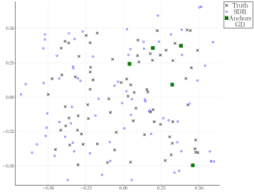
(a) The graphic result of GD initialized by an SDR solution

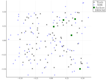
(b) The graphic result of DRSOM initialized by an SDR solution

Figure 1: Comparison of localization by GD and DRSOM with SDR initialization. The rectangles and crosses represent the anchors and true locations, respectively. The blue circles are solutions by SDR, and the red circles are final solutions of GD/DRSOM.

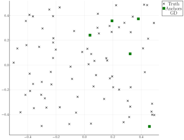
(a) The graphic result of GD without an SDR solution

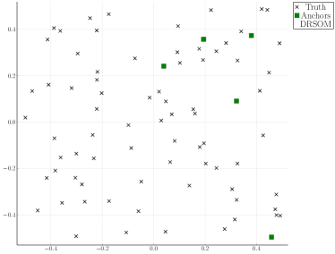
(b) The graphic result of DRSOM without an SDR solution

Figure 2: Comparison of localization by GD and DRSOM without SDR initialization. The meaning of each symbol is the same as Figure 1.

As a comparison, Figure 2 depicts the case without solving SDR first. We use the same parameter settings as for the previous case. The GD and DRSOM initializes with $X_{i}:=0,i=1,...,n$ and both solves to $\|\nabla f(x_{k})\|\leq 1e^{-6}$. In this very particular case, the GD fails to recover true positions; however, the DRSOM can provide accurate solutions even without the initialization of SDR.

In this example, we rigorously provide a case where the DRSOM may result in a better solution (in this case, the global one) than the first-order methods despite that we only have optimal subspace guarantees in theory.

4.2.2 Solving large SNL instances

In this part, we compare GD, CG, LBFGS and DRSOM on large SNL instances up to 10,000 sensors. Similar to the previous tests, CG, LBFGS and GD are facilitated with Hager-Zhang line search algorithm. We terminate an algorithm if $\|\nabla f(x_{k})\|\leq 1e^{-5}$ or the running time exceeds 3,000 seconds.

Our results are presented in Table 2. The GD fails to converge if the number of sensors exceeds 3,000, so we do not try it on larger problems. In all instances, DRSOM stands out in running time and has a clear advantage over CG and LBFGS. Notably, it successfully solves the problem with 10,000 sensors to $\|\nabla f(x_{k})\|\leq 1e^{-5}$ in about 2,200 seconds while all other competing algorithms fail.

Table 2: Results of CG, LBFGS, DRSOM, and GD on SNL instances. $n$ and $m$ denotes the number of sensors and anchors. $|E|$ denotes the number of used edges (QCQP constraints).

$n$	$m$	$|E|$	$k$
			CG	LBFGS	DRSOM	GD
500	50	2.2e+04	1.2e+02	9.5e+01	9.0e+01	3.2e+02
1000	80	4.6e+04	2.3e+02	2.1e+02	2.1e+02	1.4e+03
2000	120	9.4e+04	4.5e+02	3.8e+02	3.6e+02	4.4e+03
3000	150	1.4e+05	7.4e+02	5.6e+02	5.4e+02	7.5e+03
4000	400	1.8e+05	1.2e+03	5.7e+02	7.8e+02	-
6000	600	2.7e+05	1.2e+03	1.1e+03	1.1e+03	-
10000	1000	4.5e+05	1.0e+03	9.7e+02	1.5e+03	-

(a) Iteration number

$n$	$m$	$|E|$	$\|g\|$
			CG	LBFGS	DRSOM	GD
500	50	2.2e+04	7.0e-06	8.9e-06	6.8e-06	9.4e-06
1000	80	4.6e+04	7.0e-06	8.3e-06	8.6e-06	9.9e-06
2000	120	9.4e+04	8.4e-06	8.5e-06	8.4e-06	9.9e-06
3000	150	1.4e+05	8.9e-06	9.3e-06	8.4e-06	1.6e-03∗
4000	400	1.8e+05	7.9e-06	8.9e-06	9.8e-06	-
6000	600	2.7e+05	9.2e-06	9.9e-06	8.8e-06	-
10000	1000	4.5e+05	2.3e-03∗	1.0e-04∗	9.0e-06	-

(b) Gradient norm at termination. Symbol “*” means the algorithm does not attain the required accuracy.

$n$	$m$	$|E|$	$t$
			CG	LBFGS	DRSOM	GD
500	50	2.2e+04	1.7e+01	1.3e+01	1.1e+01	2.3e+01
1000	80	4.6e+04	7.3e+01	6.2e+01	3.9e+01	1.8e+02
2000	120	9.4e+04	2.5e+02	2.5e+02	1.4e+02	1.1e+03
3000	150	1.4e+05	6.5e+02	5.8e+02	2.7e+02	-
4000	400	1.8e+05	1.3e+03	7.2e+02	5.0e+02	-
6000	600	2.7e+05	2.0e+03	2.1e+03	1.1e+03	-
10000	1000	4.5e+05	-	-	2.2e+03	-

(c) Running time. Symbol “-” means the algorithm reaches 3,000s

4.3 CUTEst Benchmark

In this subsection, we test DRSOM in a nonlinear programming benchmark CUTEst dataset [21]. Besides, we report results of first-order methods including GD and CG, and second-order methods including Newton-TR and LBFGS. Similar to the previous tests, CG, LBFGS and GD are facilitated with Hager-Zhang line search algorithm. Since each problem in the CUTEst dataset may have multiple different realizations by possibly multiple parameters, we enumerate these combinations and choose the first one that has $n\leq 200$ variables.

We use the nonlinear programming interface in Julia programming language facilitated by open source infrastructure [32] for DRSOM and all other competing algorithms. We report an overall comparison in Table 3, where we present average values of iteration number $\overline{k}$, function $\overline{k}^{f}$, gradient $\overline{k}^{g}$ and Hessian $\overline{k}^{H}$ evaluations. Besides, we also provide the scaled geometric mean as an extra metric including $\overline{k}_{G}$, $\overline{k}_{G}^{f}$, $\overline{k}_{G}^{g}$, $\overline{k}_{G}^{H}$ correspondingly. We report CPU time $\overline{t},\overline{t}_{G}$ in both measures. We mark an instance successfully solved if the returned iterate $x_{k}$ satisfies $\min\{\|g_{k}\|,\|g_{k}\|/\|g_{0}\|\}\leq 1e^{-5}$, where $g_{0}$ is the gradient at the initial point $x_{0}$. The minimum we use here accounts for the case where the gradient is too large, in which case a solution is acceptable in a relative measure. Under such a criterion, we count the total number of successful instances as $\mathcal{K}$.

Note that the Hessian-vector products are already available in [32], so DRSOM directly takes advantage of HVP computations. To this end, the metric $\overline{k}_{G}^{g}$ also includes number of needed HVP as extra gradient evaluations (counted as 2 per each call). We scale geometric mean for time and all other evaluations number by 1 (second) and 50 (iterations), respectively. We report detailed results in Appendix A.

Table 3: Performance of different algorithms on the CUTEst dataset. Note $\overline{t},\overline{k}$ are mean running time and iteration; $\overline{t}_{G},\overline{k}_{G}$ are scaled geometric means (scaled by 1 second and 50 iterations, respectively). If an instance is the failed, its iteration number and solving time are set to $20,000$.

method	$\mathcal{K}$	$\overline{t}$	$\overline{k}$	$\overline{k}^{f}$	$\overline{k}^{g}$	$\overline{k}^{H}$
LBFGS	96.00	0.18	583.53	1680.79	1680.79	0.00
Newton-TR	94.00	1.38	2636.71	927.78	2637.71	875.96
CG	98.00	0.45	1193.41	12374.70	12374.70	0.00
DRSOM	97.00	0.20	1163.92	1206.06	3519.81	0.00
GD	91.00	1.33	6007.38	24602.65	24602.65	0.00

(a) Performance in algebraic averages

method	$\overline{t}_{G}$	$\overline{k}_{G}$	$\overline{k}_{G}^{f}$	$\overline{k}_{G}^{g}$	$\overline{k}_{G}^{H}$
LBFGS	0.08	76.39	180.59	180.59	-0.00
Newton-TR	0.29	99.34	43.84	101.30	40.35
CG	0.09	124.73	282.38	282.38	-0.00
DRSOM	0.09	133.10	162.42	332.32	-0.00
GD	0.32	952.60	1947.67	1947.67	-0.00

(b) Performance in geometric averages

From Table 3, we can see that the quasi-Newton method LBFGS stands out in terms of iteration number, while CG has the most successful instances. However, we observe that DRSOM is exceptional using only 2D subspace with gradient and momentum. This observation becomes more evident in average CPU time $\overline{t}$ and evaluation numbers. Not surprisingly, Table 3 indicates that DRSOM has a clear advantage over the gradient method, since DRSOM solves more instances and tends to be more stable, as seen from scaled metrics with subscript $G$. Besides, the average running time of DRSOM is better than CG, but these two methods should be close in terms of scaled metrics. We highlight a comparison of DRSOM with LBFGS (with a Hager-Zhang line-search algorithm), which clearly demonstrates the benefits of using second-order information even in a very limited manner. As the current implementation of DRSOM already demonstrates a saving in function and gradient evaluations, it is reasonable to expect better numerical routines can further improve these benchmark results. This of course serves as one of our future directions.

5 Conclusion

In this paper, we introduce a Dimension-Reduced Second-Order Method (DRSOM) that utilizes 2-D trust-region subproblems and requires only the gradient, momentum and two extra Hessian-vector products (alternatively, interpolation with three function evaluations) that cost almost the same as first-order methods. We give a concise analysis of the global and local speed of convergence. Computationally, we provide fruitful examples in nonconvex optimization. Notably, DRSOM has substantial superiority to first-order methods while keeping a low cost per iteration compared to second-order methods.

Our preliminary results motivate future developments of DRSOM. In terms of Assumption 2, it is an important aspect to find more efficient approach to satisfy (18) in addition to the Krylov-like corrector method algorithm 2.

Appendix A Detailed Computational Results for CUTEst Dataset

Table 4: Complete Results on CUTEst Dataset, iteration & time

	method	CG		DRSOM		GD		LBFGS		Newton-TR
		$k$	$t$	$k$	$t$	$k$	$t$	$k$	$t$	$k$	$t$
name	n
ARGLINA	200	1	4.5e-04	2	1.0e-03	1	4.4e-04	1	6.1e-04	5	4.9e-01
ARGLINB	200	1	4.7e-04	2	2.0e-03	1	5.7e-04	3	1.5e-03	4	3.8e-01
ARGLINC	200	1	4.4e-04	2	2.0e-03	1	5.1e-04	4	2.4e-03	4	3.4e-01
ARGTRIGLS	200	1151	8.7e-01	611	1.0e+00	20000	1.7e+01	541	6.4e-01	12	1.2e+00
ARWHEAD	100	18	8.2e-04	10	3.0e-03	57	2.6e-03	6	5.6e-04	5	5.1e-03
BDQRTIC	100	136	6.4e-03	138	2.1e-02	3701	1.5e-01	30	1.5e-03	10	1.8e-02
BOX	10	7	1.9e-04	4	0.0e+00	60	6.3e-04	4	2.7e-04	2	3.6e-04
BOXPOWER	10	59	6.1e-04	19	1.0e-03	20000	1.3e-01	15	6.0e-04	11	5.9e-04
BROWNAL	200	5	8.9e-03	5	1.1e-02	102	6.6e-02	4	5.9e-03	6	5.6e-01
BROYDN3DLS	50	25	4.4e-04	30	3.0e-03	62	8.3e-04	24	7.4e-04	5	2.3e-03
BROYDN7D	50	85	3.0e-03	82	9.0e-03	167	4.9e-03	63	2.5e-03	15	6.8e-03
BROYDNBDLS	50	113	2.5e-03	102	1.1e-02	996	2.5e-02	61	2.0e-03	10	4.8e-03
BRYBND	50	113	2.9e-03	102	1.4e-02	996	2.1e-02	61	2.0e-03	10	4.4e-03
CHAINWOO	4	201	1.4e-03	326	1.6e-02	6053	2.7e-02	21	3.2e-04	45	8.5e-04
CHNROSNB	25	352	3.8e-03	322	2.0e-02	4754	5.8e-02	109	1.6e-03	40	4.2e-03
CHNRSNBM	25	361	4.0e-03	374	2.4e-02	6252	6.5e-02	171	2.4e-03	45	4.8e-03
COSINE	100	2	1.8e-04	2	0.0e+00	2	4.6e-04	10	9.3e-04	12	2.8e-02
CRAGGLVY	50	96	3.4e-03	87	1.3e-02	330	1.4e-02	71	2.6e-03	17	6.3e-03
CURLY10	100	1274	4.1e-02	820	5.5e-02	17334	5.4e-01	809	2.5e-02	12	2.1e-02
CURLY20	100	1306	5.6e-02	933	6.7e-02	20000	8.9e-01	882	3.4e-02	12	2.5e-02
DIXMAANA	90	7	3.6e-04	8	2.0e-03	7	2.8e-04	5	5.4e-04	7	1.7e-02
DIXMAANB	90	8	4.1e-04	9	2.0e-03	9	3.5e-04	6	6.1e-04	12	7.5e-02
DIXMAANC	90	9	4.7e-04	10	2.0e-03	9	5.2e-04	6	5.0e-04	10	1.5e-02
DIXMAAND	90	10	5.2e-04	10	2.0e-03	11	7.1e-04	8	5.8e-04	12	1.8e-02
DIXMAANE	90	43	2.5e-03	47	7.0e-03	364	1.6e-02	42	1.7e-03	8	1.2e-02
DIXMAANF	90	43	2.5e-03	49	8.0e-03	362	1.7e-02	37	1.6e-03	15	2.0e-02
DIXMAANG	90	44	2.6e-03	49	8.0e-03	324	1.3e-02	35	1.6e-03	13	2.0e-02
DIXMAANH	90	42	2.5e-03	49	8.0e-03	355	1.4e-02	37	1.6e-03	15	2.6e-02
DIXMAANI	90	151	8.8e-03	155	2.4e-02	14646	6.5e-01	154	5.9e-03	10	1.3e-02
DIXMAANJ	90	136	8.0e-03	142	2.0e-02	12973	6.9e-01	138	5.5e-03	17	3.0e-02
DIXMAANK	90	137	8.2e-03	134	1.6e-02	13414	6.0e-01	138	5.4e-03	16	3.3e-02
DIXMAANL	90	121	7.1e-03	129	1.7e-02	13357	6.9e-01	138	5.3e-03	17	2.2e-02
DIXMAANM	90	161	1.9e-02	162	1.2e+00	15424	7.4e-01	160	8.6e-01	8	2.8e-01
DIXMAANN	90	202	1.2e-02	202	2.5e-02	14490	7.1e-01	167	6.4e-03	20	2.9e-02
DIXMAANO	90	147	8.6e-03	202	2.4e-02	14655	7.6e-01	181	7.0e-03	19	5.7e-02
DIXMAANP	90	149	8.9e-03	188	2.4e-02	14575	7.6e-01	136	5.3e-03	26	3.3e-02
DIXON3DQ	100	100	1.9e-03	102	1.1e-02	20000	3.1e-01	100	2.2e-03	5	9.1e-03
DQDRTIC	50	5	1.9e-04	9	1.0e-03	1333	2.8e-02	5	4.6e-04	5	1.5e-03
DQRTIC	50	14	3.1e-04	16	1.0e-03	14	3.3e-04	31	6.4e-04	25	4.7e-03
EDENSCH	36	30	8.0e-04	27	3.0e-03	44	1.6e-03	21	6.6e-04	15	4.1e-03
EIGENALS	6	17	3.7e-04	7	1.0e-03	349	1.9e-03	9	3.6e-04	7	4.6e-04
EIGENBLS	6	32	2.6e-04	30	2.0e-03	282	3.0e-03	11	3.1e-04	17	1.2e-03
EIGENCLS	30	175	3.9e-03	133	1.4e-02	841	2.0e-02	126	3.4e-03	17	4.4e-03
ENGVAL1	50	24	5.8e-04	24	3.0e-03	36	5.9e-04	15	5.1e-04	9	1.1e-02
ERRINROS	25	19275	1.9e-01	6025	2.3e-01	20000	2.5e-01	94	1.5e-03	47	4.9e-03
ERRINRSM	25	20000	1.9e-01	20000	5.8e-01	20000	2.1e-01	217	2.9e-03	86	8.9e-03
EXTROSNB	100	3798	8.6e-02	2722	1.4e-01	20000	5.4e-01	5037	1.3e-01	1645	1.7e+00
FLETBV3M	10	0	8.1e-06	3	0.0e+00	0	9.5e-07	0	5.2e-05	0	5.2e-05
FLETCBV2	10	5	1.6e-04	6	1.0e-03	182	2.0e-03	5	2.7e-04	1	3.3e-04
FLETCBV3	10	0	9.1e-06	14	2.0e-03	0	6.0e-06	0	8.5e-05	0	4.8e-05
FLETCHBV	10	10	1.1e-04	20	2.0e-03	390	2.9e-03	10	3.2e-04	88	2.9e-03
FLETCHCR	100	678	3.3e-02	866	1.1e-01	20000	5.4e-01	487	1.5e-02	202	5.0e-01
FMINSRF2	16	68	6.1e-04	57	4.0e-03	983	7.5e-03	29	5.8e-04	20000	7.0e-02
FMINSURF	16	24	2.1e-04	27	3.0e-03	84	8.6e-04	21	4.2e-04	20000	1.7e+00
FREUROTH	50	97	2.6e-03	99	1.2e-02	6575	1.6e-01	16	1.0e-03	9	5.2e-03
GENHUMPS	10	362	6.8e-03	134	1.2e-02	5166	9.6e-02	421	6.0e-03	12910	6.1e-01
GENROSE	100	309	1.7e-02	272	2.8e-02	2924	9.8e-02	270	7.3e-02	95	2.0e-01
HILBERTA	6	4	1.9e-04	6	1.0e-03	2839	2.4e-02	4	2.7e-04	4	4.9e-04
HILBERTB	5	3	6.6e-05	4	0.0e+00	6	4.9e-05	3	3.4e-04	3	3.4e-04
INDEF	50	1	9.1e-06	31	3.8e-02	1	3.1e-06	1	8.5e-05	20000	9.3e+00
INDEFM	50	135	4.1e-03	152	1.5e-02	20000	7.4e-01	63	2.4e-03	28	1.5e-02
INTEQNELS	102	5	1.3e-03	6	4.0e-03	6	1.2e-03	4	1.3e-03	3	3.4e-02
JIMACK	81	12150	3.4e+01	3285	1.0e+01	20000	7.1e+01	3628	1.5e+01	20000	5.1e+01
LIARWHD	36	24	6.6e-04	12	1.0e-03	337	6.0e-03	10	3.9e-04	12	4.0e-03
MANCINO	50	9	1.2e-02	10	2.4e-02	10	1.4e-02	8	1.2e-02	11	3.3e-02
MODBEALE	10	194	2.1e-03	2222	7.5e-02	20000	2.8e-01	36	7.4e-04	8	5.5e-04
MOREBV	50	218	3.5e-03	220	1.9e-02	20000	4.3e-01	252	5.3e-03	1	5.6e-04
MSQRTALS	49	135	4.6e-03	132	2.0e-02	1184	4.5e-02	103	5.0e-03	12	1.0e-02
MSQRTBLS	49	217	7.2e-03	249	3.0e-02	3570	1.6e-01	177	7.8e-03	15	1.3e-02
NCB20	110	852	1.0e-01	731	1.9e-01	20000	6.8e+00	330	4.8e-02	75	1.9e-01
NCB20B	180	2336	4.8e-01	4710	2.2e+00	20000	1.1e+01	1154	3.5e-01	11	5.9e-02
NONCVXU2	10	50	4.0e-04	51	5.0e-03	182	1.9e-03	23	4.5e-04	20000	1.6e+00
NONCVXUN	10	29	5.4e-04	28	2.0e-03	58	5.0e-04	21	4.3e-04	20000	8.1e-01
NONDIA	90	19	6.9e-04	10	2.0e-03	7974	1.7e-01	8	4.9e-04	6	4.2e-03
NONDQUAR	100	3040	7.2e-02	7558	3.2e-01	8735	2.3e-01	666	1.7e-02	15	1.2e-01
NONMSQRT	49	20000	5.7e-01	20000	1.3e+00	20000	9.4e-01	20000	9.7e-01	20000	8.6e+00
OSCIGRAD	15	73	1.9e-03	63	5.0e-03	183	3.2e-03	45	9.4e-04	20000	3.2e+00
OSCIPATH	25	9	2.4e-04	10	2.0e-03	12	1.1e-04	9	4.5e-04	9	2.1e-03
PENALTY1	50	44	8.9e-04	37	4.0e-03	673	1.7e-02	90	1.5e-03	41	1.9e-02
PENALTY2	50	194	8.1e-03	172	2.2e-02	5765	2.2e-01	139	5.9e-03	25	1.3e-02
PENALTY3	50	84	1.6e-01	90	2.5e-01	329	6.0e-01	53	1.0e-01	17	6.0e-02
POWELLSG	60	80	1.1e-03	1017	4.6e-02	11094	1.4e-01	23	6.0e-04	16	5.2e-03
POWER	50	34	4.8e-04	31	2.0e-03	53	1.3e-03	27	5.7e-04	21	1.0e-02
QUARTC	100	16	5.4e-04	20	3.0e-03	16	4.2e-04	31	8.1e-04	29	1.6e-02
SBRYBND	50	20000	9.5e+00	20000	1.0e+00	20000	1.2e+01	20000	7.4e-01	576	3.3e-01
SCHMVETT	10	32	6.9e-04	28	2.0e-03	211	2.3e-03	17	3.9e-04	3	3.9e-04
SCOSINE	10	2	1.5e-04	2	1.0e-03	2	1.3e-04	2	3.5e-04	20000	6.9e-01
SCURLY10	10	1	1.0e-05	2	1.3e-02	1	3.1e-06	1	5.4e-05	11	9.4e-04
SENSORS	10	18	5.0e-03	19	5.0e-03	28	4.1e-03	25	2.3e-03	10	1.1e-03
SINQUAD	50	60	2.0e-03	25	4.0e-03	444	2.0e-02	12	7.3e-04	10	4.2e-03
SPARSINE	50	275	8.8e-03	320	2.9e-02	7976	2.2e-01	196	6.2e-03	28	1.3e-02
SPARSQUR	50	10	2.6e-04	13	3.0e-03	10	4.0e-04	11	6.7e-04	14	8.5e-03
SPMSRTLS	100	65	3.5e-03	65	1.3e-02	286	1.4e-02	60	3.4e-03	13	2.0e-02
SROSENBR	50	14	4.5e-04	8	1.0e-03	5273	5.2e-02	7	3.3e-04	9	2.0e-03
SSBRYBND	50	11679	6.2e-01	3751	1.8e-01	20000	3.5e+00	2528	9.2e-02	21	9.4e-03
SSCOSINE	10	8	1.0e-03	20000	4.9e-01	2	1.2e-04	2	4.2e-04	20000	5.4e-01
TOINTGSS	50	16	3.6e-04	17	3.0e-03	37	1.3e-03	16	5.8e-04	20000	1.3e+01
TQUARTIC	50	25	5.6e-04	20	3.0e-03	9119	1.6e-01	11	5.1e-04	12	4.8e-03
TRIDIA	50	52	6.0e-04	59	4.0e-03	3187	3.2e-02	52	1.0e-03	4	1.6e-03
VARDIM	200	10	7.5e-03	8	1.1e-02	4	2.7e-03	3	8.3e-04	9	4.8e-02
VAREIGVL	100	98	5.4e-03	126	2.1e-02	55	2.3e-03	21	1.3e-03	25	5.5e-02
WATSON	12	681	1.2e-02	386	3.1e-02	20000	5.3e-01	38	1.1e-03	13	1.9e-03
WOODS	4	201	1.5e-03	326	1.6e-02	6053	3.8e-02	21	3.4e-04	45	8.3e-04
YATP1LS	120	357	1.4e-01	58	2.6e-02	20000	2.8e+00	129	1.9e-02	20000	4.6e+01
YATP2LS	8	9	1.2e-04	11	2.0e-03	13	1.6e-04	8	2.9e-04	20000	5.1e-01

Table 4: Complete Results on CUTEst Dataset, iteration & time

Table 5: Complete Results on CUTEst Dataset, function value & norm of the gradient

	method	CG		DRSOM		GD		LBFGS		Newton-TR
		$\|g\|$	$f$	$\|g\|$	$f$	$\|g\|$	$f$	$\|g\|$	$f$	$\|g\|$	$f$
name	n
ARGLINA	200	4.0e-14	2.3e-26	3.0e-13	2.3e-26	4.0e-14	2.3e-26	4.0e-14	2.3e-26	5.2e-14	1.3e-26
ARGLINB	200	2.8e-03	5.0e+01	2.3e-02	5.0e+01	2.8e-03	5.0e+01	7.6e-06	5.0e+01	1.9e-03	5.0e+01
ARGLINC	200	1.5e-03	5.1e+01	1.3e-02	5.1e+01	1.5e-03	5.1e+01	7.1e-06	5.1e+01	1.5e-03	5.1e+01
ARGTRIGLS	200	9.8e-06	2.6e-12	9.4e-06	1.7e-14	4.6e-05	5.2e-10	9.0e-06	1.4e-12	4.4e-09	8.3e-20
ARWHEAD	100	8.5e-07	3.0e-12	1.2e-07	0.0e+00	7.5e-06	2.1e-11	1.4e-07	0.0e+00	6.3e-06	6.6e-14
BDQRTIC	100	7.2e-06	3.8e+02	9.4e-06	3.8e+02	1.0e-05	3.8e+02	8.0e-06	3.8e+02	4.0e-06	3.8e+02
BOX	10	4.7e-07	-1.7e-01	5.6e-06	-1.7e-01	7.3e-06	-1.7e-01	1.8e-08	-1.7e-01	2.6e-06	-1.7e-01
BOXPOWER	10	8.6e-06	1.2e-07	6.5e-06	4.3e-09	7.0e-05	3.5e-06	4.1e-08	6.0e-11	5.6e-06	1.3e-07
BROWNAL	200	4.8e-06	1.5e-09	3.8e-06	1.5e-09	9.3e-06	1.5e-09	1.6e-06	1.5e-09	4.7e-10	7.5e-20
BROYDN3DLS	50	6.9e-06	2.4e-12	9.3e-06	5.2e-13	8.0e-06	1.8e-11	5.9e-06	2.2e-12	1.0e-06	5.7e-14
BROYDN7D	50	7.6e-06	1.8e+01	9.7e-06	1.8e+01	9.8e-06	1.7e+01	6.8e-06	1.7e+01	1.9e-09	1.7e+01
BROYDNBDLS	50	1.0e-05	4.1e-12	8.7e-06	2.1e-13	9.9e-06	2.2e-11	1.0e-05	1.1e-11	4.4e-13	8.8e-18
BRYBND	50	1.0e-05	4.1e-12	8.7e-06	2.1e-13	9.9e-06	2.2e-11	1.0e-05	1.1e-11	4.4e-13	8.8e-18
CHAINWOO	4	3.5e-06	1.0e+00	9.0e-06	1.0e+00	9.9e-06	1.0e+00	2.9e-07	1.0e+00	2.7e-09	1.0e+00
CHNROSNB	25	7.1e-06	1.9e-11	7.3e-06	3.1e-12	1.0e-05	1.4e-10	3.7e-06	4.2e-13	4.6e-07	2.5e-13
CHNRSNBM	25	1.0e-05	7.3e-12	9.0e-06	3.5e-12	1.0e-05	1.3e-10	7.8e-06	2.6e-12	2.7e-09	2.0e-20
COSINE	100	8.7e+00	-1.3e+01	8.1e+01	-1.3e+01	8.7e+00	-1.3e+01	2.1e-06	-9.9e+01	2.1e-13	-9.9e+01
CRAGGLVY	50	9.6e-06	1.5e+01	8.4e-06	1.5e+01	9.9e-06	1.5e+01	9.7e-06	1.5e+01	1.6e-07	1.5e+01
CURLY10	100	2.4e-05	-1.0e+04	1.1e-04	-1.0e+04	3.3e-05	-1.0e+04	1.8e-05	-1.0e+04	3.3e-10	-1.0e+04
CURLY20	100	2.6e-05	-1.0e+04	1.5e-04	-1.0e+04	7.4e-05	-1.0e+04	3.3e-05	-1.0e+04	2.2e-10	-1.0e+04
DIXMAANA	90	3.0e-07	1.0e+00	8.7e-07	1.0e+00	2.0e-06	1.0e+00	4.8e-06	1.0e+00	6.0e-19	1.0e+00
DIXMAANB	90	3.5e-06	1.0e+00	9.8e-07	1.0e+00	3.3e-07	1.0e+00	3.1e-06	1.0e+00	2.5e-07	1.0e+00
DIXMAANC	90	2.8e-07	1.0e+00	3.6e-07	1.0e+00	1.2e-06	1.0e+00	5.2e-06	1.0e+00	5.1e-12	1.0e+00
DIXMAAND	90	2.5e-06	1.0e+00	9.0e-06	1.0e+00	4.3e-06	1.0e+00	6.9e-07	1.0e+00	4.3e-11	1.0e+00
DIXMAANE	90	6.7e-06	1.0e+00	6.7e-06	1.0e+00	9.7e-06	1.0e+00	8.3e-06	1.0e+00	1.8e-12	1.0e+00
DIXMAANF	90	7.6e-06	1.0e+00	8.6e-06	1.0e+00	9.8e-06	1.0e+00	9.7e-06	1.0e+00	2.7e-07	1.0e+00
DIXMAANG	90	7.0e-06	1.0e+00	7.5e-06	1.0e+00	9.9e-06	1.0e+00	6.6e-06	1.0e+00	1.0e-11	1.0e+00
DIXMAANH	90	9.9e-06	1.0e+00	8.8e-06	1.0e+00	9.7e-06	1.0e+00	9.2e-06	1.0e+00	2.7e-10	1.0e+00
DIXMAANI	90	8.9e-06	1.0e+00	9.4e-06	1.0e+00	1.0e-05	1.0e+00	9.6e-06	1.0e+00	3.2e-09	1.0e+00
DIXMAANJ	90	8.7e-06	1.0e+00	8.5e-06	1.0e+00	1.0e-05	1.0e+00	6.7e-06	1.0e+00	1.2e-06	1.0e+00
DIXMAANK	90	1.0e-05	1.0e+00	9.7e-06	1.0e+00	1.0e-05	1.0e+00	6.7e-06	1.0e+00	6.5e-07	1.0e+00
DIXMAANL	90	8.9e-06	1.0e+00	9.4e-06	1.0e+00	1.0e-05	1.0e+00	9.8e-06	1.0e+00	1.0e-11	1.0e+00
DIXMAANM	90	9.4e-06	1.0e+00	9.2e-06	1.0e+00	1.0e-05	1.0e+00	8.7e-06	1.0e+00	2.0e-15	1.0e+00
DIXMAANN	90	8.3e-06	1.0e+00	9.5e-06	1.0e+00	1.0e-05	1.0e+00	9.9e-06	1.0e+00	5.7e-07	1.0e+00
DIXMAANO	90	9.6e-06	1.0e+00	9.8e-06	1.0e+00	1.0e-05	1.0e+00	8.7e-06	1.0e+00	9.0e-06	1.0e+00
DIXMAANP	90	8.1e-06	1.0e+00	9.8e-06	1.0e+00	1.0e-05	1.0e+00	8.9e-06	1.0e+00	2.2e-07	1.0e+00
DIXON3DQ	100	6.3e-12	3.9e-23	8.4e-06	2.1e-12	1.5e-04	4.6e-04	5.5e-12	2.6e-23	2.5e-14	4.9e-25
DQDRTIC	50	3.2e-14	6.4e-29	4.4e-06	3.5e-12	9.9e-06	2.5e-11	4.1e-13	7.2e-27	4.5e-14	1.2e-28
DQRTIC	50	1.6e-06	1.3e-07	4.8e-06	3.4e-09	9.7e-06	9.8e-07	2.8e-06	2.3e-08	8.9e-06	4.3e-07
EDENSCH	36	5.8e-06	2.2e+02	3.0e-06	2.2e+02	9.9e-06	2.2e+02	8.7e-06	2.2e+02	6.0e-06	2.2e+02
EIGENALS	6	1.1e-07	1.6e-16	1.7e-06	9.4e-24	9.8e-06	9.1e-11	9.9e-07	1.3e-14	1.4e-06	5.6e-13
EIGENBLS	6	4.5e-06	1.8e-01	8.6e-06	1.8e-01	9.9e-06	1.8e-01	3.3e-08	1.8e-01	5.6e-09	4.9e-18
EIGENCLS	30	9.6e-06	1.2e-10	7.0e-06	5.6e-12	9.9e-06	6.1e-10	5.5e-06	4.5e-11	1.2e-07	4.8e-16
ENGVAL1	50	6.5e-06	5.4e+01	7.7e-06	5.4e+01	9.6e-06	5.4e+01	4.3e-06	5.4e+01	1.4e-08	5.4e+01
ERRINROS	25	9.2e-06	1.8e+01	9.8e-06	1.8e+01	4.0e-03	1.8e+01	9.9e-06	1.8e+01	6.9e-06	1.8e+01
ERRINRSM	25	1.5e-03	1.8e+01	1.1e-01	1.8e+01	1.4e-02	1.8e+01	9.7e-06	1.8e+01	3.7e-07	1.8e+01
EXTROSNB	100	9.9e-06	3.1e-06	8.9e-06	1.9e-06	6.8e-03	1.6e-03	8.3e-06	2.8e-09	9.7e-06	1.8e-08
FLETBV3M	10	2.4e-06	1.2e-05	5.6e-07	-2.2e-03	2.4e-06	1.2e-05	2.4e-06	1.2e-05	2.4e-06	1.2e-05
FLETCBV2	10	6.1e-09	-5.5e-01	3.6e-07	-5.5e-01	1.0e-05	-5.5e-01	6.1e-09	-5.5e-01	1.7e-15	-5.5e-01
FLETCBV3	10	2.4e-06	1.2e-05	3.5e-07	-3.2e-02	2.4e-06	1.2e-05	2.4e-06	1.2e-05	2.4e-06	1.2e-05
FLETCHBV	10	9.1e-13	-2.7e+06	2.7e-06	-2.7e+06	9.3e-06	-2.7e+06	0.0e+00	-2.7e+06	4.5e-13	-2.7e+06
FLETCHCR	100	9.3e-06	3.2e-11	9.2e-06	1.7e-12	1.0e-02	1.4e-04	6.9e-06	9.9e-13	2.5e-06	2.7e-12
FMINSRF2	16	7.0e-06	1.0e+00	9.0e-06	1.0e+00	1.0e-05	1.0e+00	5.2e-06	1.0e+00	6.5e-01	0.0e+00
FMINSURF	16	1.0e-05	1.0e+00	6.1e-06	1.0e+00	9.4e-06	1.0e+00	6.4e-06	1.0e+00	8.8e-01	3.6e+01
FREUROTH	50	4.6e-06	5.9e+03	6.3e-06	5.9e+03	3.9e-05	5.9e+03	6.0e-06	5.9e+03	7.1e-08	5.9e+03
GENHUMPS	10	3.5e-06	9.6e-11	2.4e+01	4.4e+02	4.1e-06	9.6e-11	9.6e-06	4.5e-10	2.8e-07	4.7e-13
GENROSE	100	8.0e-06	1.0e+00	5.7e-06	1.0e+00	7.2e-06	1.0e+00	6.6e-06	1.0e+00	3.8e-07	1.0e+00
HILBERTA	6	2.2e-07	5.0e-09	1.2e-06	5.0e-09	1.0e-05	1.4e-07	2.2e-07	5.0e-09	2.6e-16	4.0e-25
HILBERTB	5	2.2e-06	7.5e-13	3.9e-06	2.6e-17	8.6e-07	6.5e-14	2.2e-06	7.5e-13	2.3e-14	6.2e-29
INDEF	50	1.8e+00	4.6e+01	8.6e+00	-9.3e+14	1.8e+00	4.6e+01	1.8e+00	4.6e+01	1.1e+00	-7.2e+15
INDEFM	50	7.3e-06	-4.8e+03	8.4e-06	-4.6e+03	1.1e-04	-4.6e+03	6.7e-07	-4.9e+03	6.2e-06	-5.0e+03
INTEQNELS	102	2.5e-06	4.3e-11	1.7e-06	1.8e-15	2.6e-06	4.7e-11	6.1e-06	1.8e-10	2.5e-11	3.0e-21
JIMACK	81	9.1e-06	8.8e-01	1.0e-05	8.9e-01	1.8e-02	8.7e-01	8.8e-06	9.2e-01	1.3e+01	1.2e+00
LIARWHD	36	7.1e-07	1.0e-15	7.0e-08	7.1e-30	9.7e-06	3.3e-11	1.8e-10	2.0e-19	2.5e-09	8.2e-20
MANCINO	50	3.4e-06	8.2e-17	8.2e-07	5.2e-22	7.3e-07	3.1e-18	4.5e-08	5.2e-21	1.6e-09	6.5e-24
MODBEALE	10	6.7e-06	4.7e-11	9.8e-06	1.2e-10	4.2e-04	2.7e-07	2.5e-07	4.8e-16	1.4e-07	7.9e-15
MOREBV	50	4.2e-06	8.2e-10	7.2e-06	7.6e-10	1.0e-05	6.0e-06	8.3e-06	1.5e-08	5.8e-06	6.4e-09
MSQRTALS	49	9.6e-06	1.1e-10	9.3e-06	1.3e-11	9.9e-06	3.4e-09	1.0e-05	5.1e-10	6.0e-08	1.3e-14
MSQRTBLS	49	8.5e-06	2.1e-10	9.7e-06	4.2e-11	1.0e-05	1.3e-08	7.0e-06	2.7e-10	5.2e-08	9.9e-15
NCB20	110	6.6e-06	1.8e+02	1.0e-05	1.8e+02	3.9e-04	1.9e+02	9.4e-06	1.8e+02	4.1e-06	1.8e+02
NCB20B	180	8.6e-06	3.5e+02	1.0e-05	3.5e+02	1.2e-04	3.5e+02	9.6e-06	3.5e+02	4.7e-06	3.5e+02
NONCVXU2	10	4.4e-06	2.3e+01	9.5e-06	2.3e+01	9.6e-06	2.3e+01	3.4e-06	2.3e+01	7.7e-01	2.3e+01
NONCVXUN	10	3.4e-06	2.3e+01	9.8e-06	2.3e+01	6.8e-06	2.3e+01	3.7e-06	2.3e+01	7.2e-04	2.6e+01
NONDIA	90	3.9e-07	3.9e-15	7.3e-09	5.0e-28	1.0e-05	9.0e-12	3.1e-08	2.8e-18	1.5e-07	4.1e-18
NONDQUAR	100	9.6e-06	5.6e-07	1.0e-05	1.6e-08	1.0e-05	4.0e-05	1.0e-05	1.9e-06	4.7e-06	2.7e-09
NONMSQRT	49	1.9e-02	1.1e+00	7.8e-02	1.1e+00	1.0e-02	1.2e+00	2.8e-03	1.1e+00	1.0e-01	1.1e+00
OSCIGRAD	15	5.3e-06	2.8e-09	8.7e-06	2.8e-09	9.6e-06	2.8e-09	3.4e-06	2.8e-09	2.3e-04	1.2e-09
OSCIPATH	25	4.7e-06	1.0e+00	3.8e-06	1.0e+00	4.6e-06	1.0e+00	3.8e-06	1.0e+00	1.3e-12	1.0e+00
PENALTY1	50	6.3e-06	4.3e-04	1.6e-06	4.3e-04	8.2e-06	4.3e-04	2.6e-06	4.3e-04	8.7e-06	4.3e-04
PENALTY2	50	9.3e-06	4.3e+00	3.1e-06	4.3e+00	1.0e-05	4.3e+00	6.5e-06	4.3e+00	2.2e-10	4.3e+00
PENALTY3	50	9.2e-06	1.0e-03	8.0e-06	1.0e-03	9.1e-06	1.0e-03	8.6e-06	1.0e-03	7.5e-07	1.0e-03
POWELLSG	60	6.1e-06	2.5e-07	9.9e-06	1.4e-09	1.0e-05	7.1e-07	8.1e-06	9.0e-11	3.2e-06	5.7e-08
POWER	50	9.0e-06	3.1e-08	6.0e-06	2.3e-09	7.1e-06	2.1e-08	7.8e-06	4.6e-09	3.8e-06	6.7e-09
QUARTC	100	9.7e-06	3.1e-06	8.5e-06	1.2e-08	9.8e-06	2.8e-06	6.6e-06	6.2e-08	4.9e-06	4.4e-07
SBRYBND	50	7.2e+05	6.5e+02	1.6e+04	2.8e+02	8.0e+04	7.4e+02	4.2e+05	4.5e+02	4.1e-06	3.7e-13
SCHMVETT	10	7.9e-06	-2.4e+01	9.2e-06	-2.4e+01	9.7e-06	-2.4e+01	3.8e-07	-2.4e+01	1.8e-13	-2.4e+01
SCOSINE	10	2.0e+14	6.4e-01	2.0e+14	6.4e-01	3.4e+13	7.8e-01	3.4e+13	7.8e-01	5.3e+04	-6.8e+00
SCURLY10	10	1.1e+26	4.2e+26	4.4e+97	4.2e+26	1.1e+26	4.2e+26	1.1e+26	4.2e+26	1.0e+21	8.4e+19
SENSORS	10	4.3e-06	-2.1e+01	7.8e-06	-2.1e+01	3.0e-06	-2.1e+01	1.3e-06	-2.1e+01	4.0e-08	-2.0e+01
SINQUAD	50	7.7e-06	-1.1e+03	9.4e-06	-2.0e+02	9.9e-06	-1.1e+03	3.1e-08	-1.1e+03	8.3e-10	-1.1e+03
SPARSINE	50	7.4e-06	9.2e-12	9.2e-06	1.5e-12	1.0e-05	4.1e-11	8.8e-06	1.1e-11	5.9e-10	1.4e-19
SPARSQUR	50	9.4e-06	1.1e-07	5.6e-07	9.2e-11	3.0e-06	2.2e-08	9.1e-06	1.1e-07	6.9e-06	6.3e-08
SPMSRTLS	100	6.9e-06	3.3e-10	9.1e-06	1.5e-11	9.9e-06	1.6e-09	8.5e-06	3.0e-10	5.3e-07	4.8e-14
SROSENBR	50	6.9e-06	9.1e-12	5.3e-11	3.4e-21	1.0e-05	2.0e-09	3.3e-06	2.6e-10	9.7e-09	2.1e-18
SSBRYBND	50	8.6e-06	2.1e-13	9.6e-06	1.2e-14	1.8e+02	4.7e+01	9.1e-06	8.9e-14	1.8e-09	1.1e-17
SSCOSINE	10	1.1e+11	-7.0e+00	8.1e+02	-8.9e+00	1.5e+07	-1.1e+00	1.5e+07	-1.1e+00	3.5e+02	-6.9e+00
TOINTGSS	50	9.2e-06	1.0e+01	8.0e-06	1.0e+01	8.6e-06	1.0e+01	5.0e-06	1.0e+01	1.5e+00	1.1e+01
TQUARTIC	50	8.5e-07	1.8e-13	6.9e-08	5.9e-14	1.0e-05	6.5e-09	2.9e-06	1.2e-14	1.7e-12	1.2e-25
TRIDIA	50	3.2e-06	1.5e-13	7.8e-06	7.8e-14	1.0e-05	5.1e-11	3.2e-06	1.5e-13	1.7e-14	1.4e-29
VARDIM	200	2.3e+10	8.8e+09	6.9e+10	8.9e+08	1.4e+10	4.4e+09	4.7e+10	2.3e+10	7.8e+10	4.5e+10
VAREIGVL	100	9.9e-06	1.9e-09	9.8e-06	1.6e-10	7.7e-06	1.2e-10	7.3e-06	5.5e-11	7.7e-09	1.2e-17
WATSON	12	7.8e-06	2.3e-07	7.3e-06	1.6e-07	2.7e-04	1.1e-05	1.1e-06	1.6e-07	1.9e-06	3.2e-07
WOODS	4	3.5e-06	1.4e-12	9.0e-06	3.5e-12	9.9e-06	1.7e-10	2.9e-07	1.4e-16	2.7e-09	1.2e-19
YATP1LS	120	2.9e-06	3.8e-08	9.0e-06	6.7e-18	6.2e-03	4.3e-02	1.3e-07	1.7e-17	9.8e+01	8.0e+01
YATP2LS	8	2.9e-06	7.5e-13	6.1e-07	3.0e-16	2.4e-06	3.6e-13	1.1e-09	9.4e-20	4.0e-02	1.0e-04

Table 5: Complete Results on CUTEst Dataset, function value & norm of the gradient

References

- Apidopoulos et al. [2022] Vassilis Apidopoulos, Nicolò Ginatta, and Silvia Villa. Convergence rates for the heavy-ball continuous dynamics for non-convex optimization, under Polyak–Łojasiewicz condition. Journal of Global Optimization, 84(3):563–589, November 2022.
- Berahas et al. [2020] Albert S. Berahas, Raghu Bollapragada, and Jorge Nocedal. An investigation of Newton-Sketch and subsampled Newton methods. Optimization Methods and Software, 35(4):661–680, July 2020.
- Biswas and Ye [2004] Pratik Biswas and Yinyu Ye. Semidefinite programming for ad hoc wireless sensor network localization. In Third International Symposium on Information Processing in Sensor Networks, IPSN 2004, pages 46–54, 2004.
- Carmon et al. [2017] Yair Carmon, Oliver Hinder, John C. Duchi, and Aaron Sidford. Convex Until Proven Guilty: Dimension-Free Acceleration of Gradient Descent on Non-Convex Functions, May 2017.
- Carmon et al. [2018] Yair Carmon, John C. Duchi, Oliver Hinder, and Aaron Sidford. Accelerated Methods for NonConvex Optimization. SIAM Journal on Optimization, 28(2):1751–1772, January 2018.
- Cartis et al. [2010] C. Cartis, N. I. M. Gould, and Ph. L. Toint. On the Complexity of Steepest Descent, Newton’s and Regularized Newton’s Methods for Nonconvex Unconstrained Optimization Problems. SIAM Journal on Optimization, 20(6):2833–2852, January 2010.
- Cartis et al. [2011a] Coralia Cartis, Nicholas I. M. Gould, and Philippe L. Toint. Adaptive cubic regularisation methods for unconstrained optimization. Part II: worst-case function- and derivative-evaluation complexity. Mathematical Programming, 130(2):295–319, December 2011a.
- Cartis et al. [2011b] Coralia Cartis, Nicholas I. M. Gould, and Philippe L. Toint. Adaptive cubic regularisation methods for unconstrained optimization. Part I: motivation, convergence and numerical results. Mathematical Programming, 127(2):245–295, April 2011b.
- Chen [2012] Xiaojun Chen. Smoothing methods for nonsmooth, nonconvex minimization. Mathematical Programming, 134(1):71–99, August 2012.
- Chen et al. [2014] Xiaojun Chen, Dongdong Ge, Zizhuo Wang, and Yinyu Ye. Complexity of unconstrained minimization. Mathematical Programming, 143(1-2):371–383, February 2014.
- Conn et al. [2009a] A. R. Conn, Katya Scheinberg, and Luis N. Vicente. Introduction to derivative-free optimization. Number 8 in MPS-SIAM series on optimization. Society for Industrial and Applied Mathematics/Mathematical Programming Society, Philadelphia, 2009a.
- Conn et al. [2000] Andrew R. Conn, Nicholas IM Gould, and Philippe L. Toint. Trust region methods. SIAM, 2000.
- Conn et al. [2008] Andrew R. Conn, Katya Scheinberg, and Luís N. Vicente. Geometry of interpolation sets in derivative free optimization. Mathematical programming, 111(1):141–172, 2008.
- Conn et al. [2009b] Andrew R. Conn, Katya Scheinberg, and Luís N. Vicente. Global convergence of general derivative-free trust-region algorithms to first-and second-order critical points. SIAM Journal on Optimization, 20(1):387–415, 2009b.
- Curtis et al. [2017] Frank E. Curtis, Daniel P. Robinson, and Mohammadreza Samadi. A trust region algorithm with a worst-case iteration complexity of for nonconvex optimization. Mathematical Programming, 162(1):1–32, March 2017.
- Curtis et al. [2022] Frank E. Curtis, Michael J. O’Neill, and Daniel P. Robinson. Worst-Case Complexity of an SQP Method for Nonlinear Equality Constrained Stochastic Optimization, January 2022.
- Dembo et al. [1982] Ron S. Dembo, Stanley C. Eisenstat, and Trond Steihaug. Inexact Newton Methods. SIAM Journal on Numerical Analysis, 19(2):400–408, April 1982.
- Dennis and Moré [1977] John E. Dennis and Jorge J. Moré. Quasi-Newton methods, motivation and theory. SIAM review, 19(1):46–89, 1977.
- Ge et al. [2011] Dongdong Ge, Xiaoye Jiang, and Yinyu Ye. A note on the complexity of Lp minimization. Mathematical Programming, 129(2):285–299, 2011.
- Ghadimi et al. [2015] Euhanna Ghadimi, Hamid Reza Feyzmahdavian, and Mikael Johansson. Global convergence of the Heavy-ball method for convex optimization. In 2015 European Control Conference (ECC), pages 310–315, Linz, Austria, July 2015.
- Gould et al. [2015] Nicholas I. M. Gould, Dominique Orban, and Philippe L. Toint. CUTEst: a Constrained and Unconstrained Testing Environment with safe threads for mathematical optimization. Computational Optimization and Applications, 60(3):545–557, April 2015.
- Gould and Simoncini [2020] Nicholas IM Gould and Valeria Simoncini. Error estimates for iterative algorithms for minimizing regularized quadratic subproblems. Optimization Methods and Software, 35(2):304–328, 2020.
- Hager and Zhang [2006] William W. Hager and Hongchao Zhang. Algorithm 851: CG_descent, a conjugate gradient method with guaranteed descent. ACM Transactions on Mathematical Software (TOMS), 32(1):113–137, 2006.
- Kingma and Ba [2014] Diederik P. Kingma and Jimmy Ba. Adam: A method for stochastic optimization. arXiv preprint arXiv:1412.6980, 2014.
- Lacotte et al. [2021] Jonathan Lacotte, Yifei Wang, and Mert Pilanci. Adaptive newton sketch: Linear-time optimization with quadratic convergence and effective hessian dimensionality. In International Conference on Machine Learning, pages 5926–5936. 2021.
- Liu et al. [2021] Xin Liu, Zaiwen Wen, and Yaxiang Yuan. Subspace Methods for Nonlinear Optimization, 2021.
- Luenberger and Ye [2021] David G. Luenberger and Yinyu Ye. Linear and Nonlinear Programming, volume 228 of International Series in Operations Research & Management Science. Springer International Publishing, Cham, 2021.
- Nesterov [2018] Yurii Nesterov. Lectures on convex optimization, volume 137. Springer, 2018.
- Nesterov and Polyak [2006] Yurii Nesterov and B.T. Polyak. Cubic regularization of Newton method and its global performance. Mathematical Programming, 108(1):177–205, August 2006.
- Nocedal and Wright [2006] Jorge Nocedal and Stephen Wright. Numerical optimization. Springer Science & Business Media, 2006.
- Ochs et al. [2014] Peter Ochs, Yunjin Chen, Thomas Brox, and Thomas Pock. ipiano: Inertial proximal algorithm for nonconvex optimization. SIAM Journal on Imaging Sciences, 7(2):1388–1419, 2014.
- Orban and Siqueira [2019] Dominique Orban and Abel Siqueira. JuliaSmoothOptimizers, April 2019.
- Pilanci and Wainwright [2017] Mert Pilanci and Martin J. Wainwright. Newton sketch: A near linear-time optimization algorithm with linear-quadratic convergence. SIAM Journal on Optimization, 27(1):205–245, 2017.
- Polyak [1964] B. T. Polyak. Some methods of speeding up the convergence of iteration methods. USSR Computational Mathematics and Mathematical Physics, 4(5):1–17, January 1964.
- Sun et al. [2019a] Tao Sun, Dongsheng Li, Zhe Quan, Hao Jiang, Shengguo Li, and Yong Dou. Heavy-ball algorithms always escape saddle points. arXiv preprint arXiv:1907.09697, 2019a.
- Sun et al. [2019b] Tao Sun, Penghang Yin, Dongsheng Li, Chun Huang, Lei Guan, and Hao Jiang. Non-Ergodic Convergence Analysis of Heavy-Ball Algorithms. Proceedings of the AAAI Conference on Artificial Intelligence, 33(01):5033–5040, July 2019b.
- Wang and Yuan [2006] Zhou-Hong Wang and Ya-Xiang Yuan. A subspace implementation of quasi-Newton trust region methods for unconstrained optimization. Numerische Mathematik, 104(2):241–269, August 2006.
- Wang et al. [2008] Zizhuo Wang, Song Zheng, Yinyu Ye, and Stephen Boyd. Further relaxations of the semidefinite programming approach to sensor network localization. SIAM Journal on Optimization, 19(2):655–673, 2008.
- Woodruff [2014] David P. Woodruff. Sketching as a tool for numerical linear algebra. Foundations and Trends® in Theoretical Computer Science, 10(1–2):1–157, 2014.
- Xu et al. [2020] Peng Xu, Fred Roosta, and Michael W. Mahoney. Newton-type methods for non-convex optimization under inexact Hessian information. Mathematical Programming, 184(1-2):35–70, November 2020.
- Yang et al. [2021] Minghan Yang, Dong Xu, Qiwen Cui, Zaiwen Wen, and Pengxiang Xu. NG+ : A Multi-Step Matrix-Product Natural Gradient Method for Deep Learning, June 2021.
- Yang et al. [2022] Minghan Yang, Dong Xu, Zaiwen Wen, Mengyun Chen, and Pengxiang Xu. Sketch-Based Empirical Natural Gradient Methods for Deep Learning. Journal of Scientific Computing, 92(3):94, September 2022.
- Ye [1991] Yinyu Ye. A New Complexity Result on Minimization of a Quadratic Function with a Sphere Constraint. In Recent Advances in Global Optimization, volume 176, pages 19–31. Princeton University Press, 1991.
- Ye [2005] Yinyu Ye. Second Order Optimization Algorithms I, 2005.
- Yuan and Stoer [1995] Y.-X. Yuan and J. Stoer. A subspace study on conjugate gradient algorithms. ZAMM-Journal of Applied Mathematics and Mechanics/Zeitschrift für Angewandte Mathematik und Mechanik, 75(1):69–77, 1995.
- Yuan [2014] Ya-xiang Yuan. A review on subspace methods for nonlinear optimization. In Proceedings of the International Congress of Mathematics, pages 807–827, 2014.
- Yuan [2015] Ya-xiang Yuan. Recent advances in trust region algorithms. Mathematical Programming, 151(1):249–281, 2015.
- Zavriev and Kostyuk [1993] SK Zavriev and FV Kostyuk. Heavy-ball method in nonconvex optimization problems. Computational Mathematics and Modeling, 4(4):336–341, 1993.
- Zhang and Hager [2004] Hongchao Zhang and William W. Hager. A nonmonotone line search technique and its application to unconstrained optimization. SIAM journal on Optimization, 14(4):1043–1056, 2004.