Accelerating Multi-Model Bayesian Inference, Model Selection and Systematic Studies for Gravitational Wave Astronomy

Abstract

Gravitational wave models are used to infer the properties of black holes in merging binaries from the observed gravitational wave signals through Bayesian inference. Although we have access to a large collection of signal models that are sufficiently accurate to infer the properties of black holes, for some signals, small discrepancies in the models lead to systematic differences in the inferred properties. In order to provide a single estimate for the properties of the black holes, it is preferable to marginalize over the model uncertainty. Bayesian model averaging is a commonly used technique to marginalize over multiple models, however, it is computationally expensive. An elegant solution is to simultaneously infer the model and model properties in a joint Bayesian analysis. In this work we demonstrate that a joint Bayesian analysis can not only accelerate but also account for model-dependent systematic differences in the inferred black hole properties. We verify this technique by analysing 100 randomly chosen simulated signals and also the real gravitational wave signal GW200129_065458. We find that not only do we infer statistically identical properties as those obtained using Bayesian model averaging, but we can sample over a set of three models on average $2.5\times$ faster. In other words, a joint Bayesian analysis that marginalizes over three models takes on average only $20\%$ more time than a single model analysis. We then demonstrate that this technique can be used to accurately and efficiently quantify the support for one model over another, thereby assisting in Bayesian model selection.

I Introduction

Since the first detection of gravitational waves (GWs) in 2015 [1], the Advanced LIGO [2] and Advanced Virgo [3] GW observatories have detected $\sim 90$ GWs originating from compact binary coalescences (CBCs) [4, 5, 6, 7, 8, 9, 10, 11]. The properties of these binaries are typically inferred through Bayesian inference [see e.g. 12, 13, 14, 15, 16, 17, 18, 19, 20, 21, 22, 23], where Bayes’ theorem is exploited in order to calculate the posterior probability distribution: the probability that the binary has a specific set of properties given the observed data. In most cases, Bayesian inference is performed by stochastically sampling over the binaries’ properties and returning a set of independent samples drawn from the posterior distribution; although see Refs. [12, 17, 19, 20, 21, 22, 23, 24, 25] for other methods. Two common stochastic sampling approaches are Markov-Chain Monte-Carlo (MCMC) [26] and Nested Sampling [27].

In order to perform Bayesian inference on GW data, a parameterised model for the GWs emitted from a CBC [28, 29, 30, 31, 32, 33, 34, 35, 36, 37, 38, 39, 40, 41, 42, 43, 44, 45, 46, 47] is required in order to evaluate the likelihood [18]. It has previously been shown that analyses that use different models can result in noticeably different posterior distributions for individual observations [see e.g. 48, 49, 50, 51, 52, 53, 54] and the population as a whole [55, 56], which is understood to be caused by underlying systematic differences in the GW models. As illustrated most recently in the third GW transient catalog (GWTC-3) [53], systematic differences in the GW models remains a limiting factor when inferring the properties of black hole binaries (BBHs) through Bayesian inference. Although there are ongoing efforts to enhance the accuracy of future GW models [see e.g. 57], systematic differences will likely remain a limiting factor for the foreseeable future.

Bayesian model selection (BMS) provides a method for choosing between posterior distributions obtained with different models. Here, the posterior distribution obtained with the single model that best describes the data is objectively selected, i.e. the model with the largest Bayesian evidence. On the other hand, Bayesian model averaging (BMA) and Bayesian model combination combine posterior distributions obtained with different models to provide a single model marginalized result. BMA calculates a weighted average of the posterior distributions obtained with the different models (see Refs. [4, 5, 53, 58, 59] and Ref. [60] for a review) and therefore inherently assumes that only one model is the true data generating model but there is an associated uncertainty as to which model it is. Bayesian model combination is similar to BMA but instead assumes that the behaviour of the true data generating model can be replicated more closely by a combination of simpler models [61]. The posterior distributions obtained with the different models are therefore combined in a variety of ways and the combination is weighted according to the probability that the specific ensemble is correct. Other techniques, including averaging the likelihood for each model at each proposed point during the sampling [62], have been developed but in general, combining/deciphering between posterior distributions obtained with different models remains a computationally expensive exercise.

A computationally cheaper solution for marginalizing over the model involves simultaneously inferring the model and model properties in a joint Bayesian analysis (JBA) [64]. This has the benefit of ensuring that all models analyse exactly the same data with identical settings, and avoids the need to calculate weights, which are often difficult to calculate robustly. Employing a JBA to marginalize over the model is not a new principle; it has been previously explored both inside [see e.g. 65, 66, 67, 68] and outside [see e.g. 69] of GW research. Specifically, Ref. [68] used a JBA to study model systematics with an emphasis on binary neutron star mergers and the binary neutron star equation of state by using MCMC methods.

In this paper we demonstrate the validity and robustness of using a JBA to marginalize over the model for BBH mergers. We show that a) waveform systematics for BBH mergers can be addressed with a JBA, b) there is a significant reduction in computational cost when using a JBA compared to applying BMA, c) a JBA can accurately and efficiently quantify the support for one model over another, including cases where different models have a different number of parameters to describe additional physics and d) a JBA can be implemented within the Nested Sampling framework. We verified our results by analysing randomly chosen simulated signals and also the real GW signal GW200129_065458. We show that not only can we obtain statistically identical results compared to applying BMA, but also that the results can be obtained $\sim 2.5\times$ faster when sampling over 3 models. This means that a JBA that marginalizes over 3 models takes on average only $20\%$ more time than a single model analysis. Similarly, we show that a single JBA can produce two distinct Bayes’ factors on average $2.6\times$ faster than traditional techniques.

This paper is organized as follows: in Section II we describe how a JBA can efficiently marginalize over the uncertainty in a set of models. In Section III we demonstrate that a JBA produces statistically identical results as those obtained when applying BMA. In Section IV we show that a JBA can address model systematics in real GW strain data and highlight that there can be subtleties in its interpretation. In Section V we highlight that a JBA has several other applications, including the potential to significantly reduce the computation of one or more Bayes’ factors. Finally we conclude with discussions in Section VI.

II Method

The properties of a system that produced an observed GW, characterised by the multi-dimensional vector $\bm{\lambda}=\{\lambda_{1},\lambda_{2},...,\lambda_{j}\}$, can be inferred through Bayesian inference. These properties are then represented by the model-dependent posterior distribution $p(\bm{\lambda}|d,m)$, which is conditional on the observed GW data $d$ and a parameterised model $m$ for the GWs emitted from the system. This model-dependent posterior distribution is calculated using Bayes’ theorem,

$$p(\bm{\lambda}|d,m)=\frac{p(\bm{\lambda}|m)\,p(d|\bm{\lambda},m)}{\mathcal{Z}},$$ (1)

where $p(\bm{\lambda}|m)$ is the probability of the system having properties $\bm{\lambda}$ given the GW model, otherwise known as the prior, $p(d|\bm{\lambda},m)$ is the probability of observing the data given the system’s properties and GW model, otherwise known as the likelihood, and $\mathcal{Z}$ is the probability of observing the data given the GW model $\mathcal{Z}=p(d|m)\equiv\int{p(\bm{\lambda}|m)\,p(d|\bm{\lambda},m)\,d\bm{\lambda}}$, otherwise known as the evidence. The model-dependent posterior distribution assumes that model $m$ is correct.

When there is an ensemble of models, $\bm{m}=\{m_{1},...,m_{i},...,m_{N}\}$, BMA can be applied to marginalize over model uncertainty,

$$p(\bm{\lambda}|d)=\sum_{i=1}^{N}{p(\bm{\lambda}|d,m_{i})\,p(m_{i}|d)},$$ (2)

where $p(m_{i}|d)$ is the model probability (the probability of the model $m_{i}$ given the data) and $N$ is the total number of models that we wish to marginalize over. By exploiting Bayes’ theorem, it can be shown that the the model probability is a function of the model’s Bayesian evidence [60, 59],

$$p(m_{i}|d)=\frac{\mathcal{Z}_{i}\,p(m_{i})}{\sum_{j=1}^{N}\mathcal{Z}_{j}\,p(m_{j})}.$$ (3)

where $p(m_{i})$ is the prior probability for the choice of model. For the case of uniform priors, $p(m_{i})=1/N\,\,\forall\,m_{i}$, BMA is simply the average of the model-dependent posterior distributions weighted by the evidence. The significant disadvantages of using BMA to marginalize over the model is that a) $p(\bm{\lambda}|d,m_{i})$ must be calculated for all models, which is computationally expensive, and b) $\mathcal{Z}_{i}$ must be robustly inferred which is often difficult to guarantee, especially for GW Bayesian inference where tails of the likelihood surface occupy a large volume in high-dimensions.

An alternative solution for marginalizing over the model is to simultaneously infer the model and model properties in a single JBA [64]. For this case, the multi-dimensional vector $\bm{\lambda}$ can be expanded to include the model, $\tilde{\bm{\lambda}}=\{\lambda_{1},\lambda_{2},...,\lambda_{j},m\}$. If the additional degree of freedom representing the choice of model is trivial for existing parameter estimation methods to explore, a JBA will at most be $N\times$ faster to compute compared to applying BMA. For the worst case scenario, where the choice of model is difficult for parameter estimation methods to explore, we expect that a JBA will take the same time to compute as applying BMA.

In general, the JBA returns a single posterior distribution on the multi-dimensional parameter space. The probability distribution for a specific dimension can then be obtained by marginalizing over the unwanted dimensions. Consequently, the model probability can be inferred from the JBA by calculating,

$$p(m|d)=\int{p(\tilde{\bm{\lambda}}|d)\,d\lambda_{1}\,d\lambda_{2}\,...,d\lambda_{j}}.$$ (4)

Although there are multiple approaches for calculating the posterior distribution [see e.g. 12, 17, 18, 19, 20, 21, 22, 23, 24, 25], the majority of Bayesian inference analyses use stochastic parameter estimation methods that return a set of discrete samples drawn from the posterior. As explained in Section 5 of Ref. [68], assuming that the total number of collected samples from a JBA is $\mathcal{N}$, $p(m_{i}|d)$ is simply,

$$p(m_{i}|d)=\frac{\mathcal{N}_{i}}{\mathcal{N}},$$ (5)

where $\mathcal{N}_{i}$ is the number of independent samples obtained with model $m_{i}$. Assuming that we have infinite time and perfect sampling, such that we have a) sufficient samples to fully explore the model parameter space and b) a reliable estimate for $\mathcal{Z}_{i}$,

$$\frac{\mathcal{N}_{i}}{\mathcal{N}}\,=\frac{\mathcal{Z}_{i}\,p(m_{i})}{\sum_{j=1}^{N}\mathcal{Z}_{j}\,p(m_{j})}.$$ (6)

We therefore expect that the JBA will return a similar posterior distribution as that obtained when applying BMA. .

III Implementation and Validation

A typical Bayesian analysis of a quasicircular BBH analyses a 15-dimensional parameter space $\bm{\lambda}$: 2 dimensions describing the component masses of the binary ($q,\mathcal{M}$), 6 describing two spin vectors of each component ($a_{1},a_{2},\theta_{1},\theta_{2},\Delta\phi,\phi_{JL})$, 2 for the binary’s inclination and phase ($\theta_{JN},\phi$), 4 for the binary’s location on the sky, distance to the source and polarisation ($\mathrm{RA},\mathrm{DEC},d_{\mathrm{L}},\psi$) and finally 1 describing the merger time of the binary ($t_{c}$). To improve convergence when stochastically sampling over the binaries’ properties, the distance to the source is often analytically marginalized over [24], see e.g. Ref. [53], through the use of a numerical look-up-table. This means that $\bm{\lambda}$ is often a 14-dimensional parameter space. Consequently, a JBA will analyse a 15-dimensional parameter space $\tilde{\bm{\lambda}}$: all of the aforementioned dimensions plus an additional dimension describing the model ($m$).

We choose to implement our JBA into the Dynesty Nested Sampling package [70] and the pBilby parameter estimation software (a parallelised version of the Bilby software [13, 14]) since they are both regularly used by the LIGO-Virgo-KAGRA (LVK) collaborations [see e.g. 51, 52]. During the sampling of our JBA, a 15-dimensional vector of model parameters is proposed at each step, including an integer representing the model $m$. As was done in Ref. [68], in order to calculate the likelihood, we first apply a mapping which selects the model based on the integer $m$, and then pass the remaining model parameters to the selected model. We therefore simultaneously explore the model and parameter space.

To validate a) our implementation and b) the robustness of using a JBA to marginalize over model uncertainty for BBH mergers, we perform a comprehensive injection and recovery analysis. We compare the posterior distributions inferred from 100 randomly chosen simulated signals to those obtained when applying BMA to the model-dependent posteriors (see Eq. 2). We also compare the computational cost of both methods.

We choose to inject GWs emitted from 100 randomly chosen BBHs into coloured-Gaussian noise from two detectors, Hanford and Livingston, with design sensitivities [2]. In this validation study we use a selection of precessing models, which we define as models that include 6 spin degrees of freedom but do not include higher-order multipoles [71]. We do not include any complete models, which we define as models that include all 6 spin degrees of freedom and higher-order multipoles, due to the large computational cost required to analyse 100 simulated signals. We therefore simulate the injected GWs with IMRPhenomXP [44] and our recovery analysis marginalizes over IMRPhenomXP, IMRPhenomTP [45] and IMRPhenomPv3 [38].

The parameters of the injected GWs were obtained through random draws of the prior used in the recovery analysis. We used a prior that is uniform over spin magnitudes and component masses, and isotropic over spin orientation, sky location and binary orientation [4, 5, 53]. The signal-to-noise ratios (SNRs) for the injected GWs ranged from 3.0 to 47.0 with 75% of the injected binaries having SNR $>8$ (a typical search threshold). To improve the convergence of the inferred results, we analytically marginalized over the luminosity distance through the use of a numerical look-up-table. The JBA extended the prior to include an equal-weighted Categorical prior for the choice of model.

For each of the 100 simulated signals, 14 comparable distributions, one for each dimension, can be inferred from both the JBA and BMA analyses. To compare each of these 1400 distributions, we calculate the Jensen-Shannon Divergence (JSD) [72]. The JSD ranges between $0\,\mathrm{bits}$ and $1\,\mathrm{bit}$, where a JSD=$0\,\mathrm{bits}$ (JSD=$1\,\mathrm{bit}$) implies statistically identical (distinct) distributions. As shown in Fig. 1, the inferred JSDs ranged between $7\times 10^{-5}\,\mathrm{bits}$ and $0.1\,\mathrm{bits}$ with median and 90% symmetric credible interval $\mathrm{JSD}=0.002^{+0.010}_{-0.001}\,\mathrm{bits}$. As described in Ref. [4], a good rule of thumb is that a JSD $<0.05\,\mathrm{bits}$ implies that the distributions are in good agreement. We find that 98% of all distributions satisfied the JSD $<0.05\,\mathrm{bits}$ constraint. Consequently, for the majority of cases, there is no statistical difference between the JMA and BMA analyses. Although 2% of the distributions are statistically different, we find that all distributions are consistent between JBA and BMA analyses. This means that the median of the BMA analysis lies within the 90% confidence interval of the JBA and vice versa. We suspect that these small statistical differences for a subset of distributions are therefore a consequence of sampling uncertainties. We discuss the individual distributions in more detail in Appendix A.

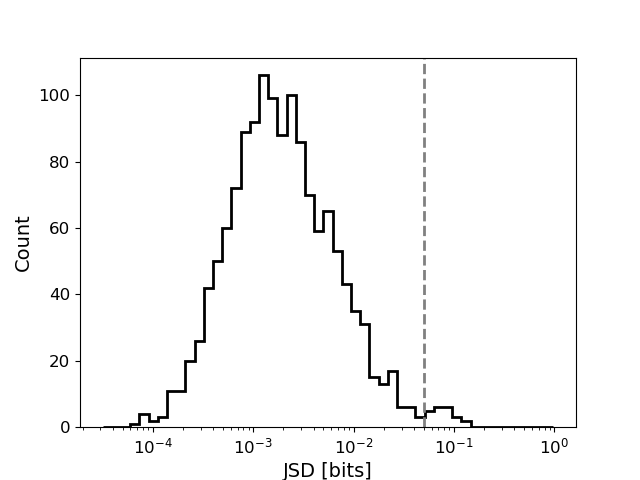
Figure 1: Comparison between the 1400 posterior distributions obtained from the JBA and BMA analyses when analysing 100 randomly chosen binaries. The Jensen-Shannon Divergence (JSD) ranges between $0\,\mathrm{bits}$ and $1\,\mathrm{bits}$ where a JSD=$0\,\mathrm{bits}$ (JSD=$1\,\mathrm{bits}$) implies statistically identical (distinct) distributions. The vertical dashed line shows a JSD$=0.05\,\mathrm{bits}$.

For the 2% of distributions with JSD $\geq 0.05\,\mathrm{bits}$, we find no correlation between the JSD and the SNR of the injected signal nor the JSD and the probability of a particular model given the data. Indeed, all distributions obtained when analysing the 14 simulated signals with the highest SNRs (ranging between 24.0 and 47.0) and the 28 simulated signals with the lowest SNRs (ranging between 3.0 and 8.0) satisfied the JSD $<0.05\,\mathrm{bits}$ constraint.

The sampling time for a Nested Sampling analysis depends on the stopping criterion; when the stopping criterion is reached, the sampling terminates and independent samples are returned. In order to gauge how computationally expensive the JBA is, we compare the total sampling time taken to analyse 100 simulated signals for both the JBA and BMA analyses when run on identical machines. The total sampling time for the JBA is the total wall clock time taken to generate $p(\tilde{\bm{\lambda}}|d)$ for each simulated signal. The total sampling time for the BMA analysis on the other hand, is the total wall clock time taken to generate $p(\bm{\lambda}|d,m_{i})$ for each model in the ensemble for each simulated signal. We found that the total sampling time to perform the JBA for 100 simulated signals was 239.5 hours with each injection taking on average 2.5 hours to complete when parallelised over 200 CPUs. Meanwhile, the total sampling time to apply BMA for 100 simulated signals was 606.5 hours when run on an identical number of CPUs.

We have therefore shown that a JBA is faster than applying BMA with no statistical difference among the obtained posterior distributions. A JBA can therefore successfully marginalize over model uncertainty for BBH mergers. However, one limitation of using a JBA is that it collects fewer independent samples: on average $2\times$ less. In general, if one model has a significantly larger model probability, we expect a comparable number of samples between the JBA and BMA analyses no matter the number of models in the ensemble. However, if all models have comparable probabilities, we expect the JBA to obtain $\sim N\times$ fewer samples than the BMA. Although this may become an issue when the JBA marginalizes over many models with comparable probabilities, this is unlikely to affect typical GW astronomy since a) ordinarily only 2 of the leading models are combined [see e.g. 4, 5, 53] and b) it is unlikely that many models will have comparable model probabilities (see e.g. Sec. IV). Consequently, for typical analyses undertaken by the LVK, a JBA can significantly reduce the computational cost of multi-model Bayesian inference.

IV Application to Bayesian Model Selection

The inferred posterior distribution from a Bayesian inference analysis is dependent on the assumed model. Owing to alternative techniques used when first constructing the models [see e.g. 73, 74, 75], some models are often more accurate than others in certain regions of the parameter space. For high SNR GW observations, these model discrepancies can show up as systematic differences in the inferred posterior distributions. This was the case for GW200129_065458 [54, 53, 76], hereafter referred to as GW200129, which was an $\mathrm{SNR}\sim 27$ signal generated by the merger of a $\sim 60\,M_{\odot}$ binary [53] and the first signal with strong evidence for spin-induced orbital precession [54].

One method for dealing with these systematic differences is to independently check the model’s accuracy by comparing it to GW signals calculated by numerically solving Einstein’s equations for a given binary system [e.g. 54]. However, it is often not feasible to apply this method since it is computationally expensive to numerically solve Einstein’s equations especially for low-mass binaries. Another method is to use BMS to identify which model has more support in the observed data. BMS objectively selects between different models by identifying the single model that has the largest Bayesian evidence, ${m}^{*}=\mathrm{max}_{m_{i}}p(d|m_{i})$.

As demonstrated in Sec. III, a JBA returns posterior distributions that are statistically identical to those obtained with BMA in a fraction of the time. This means that the inferred model probabilities from the JBA are consistent with the model’s evidence (see Eqs. 5 and 6). We therefore propose that the JBA can be used to accelerate BMS. To demonstrate this, we performed an independent analysis of GW200129 that marginalized over a selection of the latest complete models, and inferred the model probability. We chose to include NRSur7dq4 ($m_{\mathrm{NRS}}$) [40], IMRPhenomXPHM ($m_{\mathrm{XPHM}}$) and IMRPhenomTPHM ($m_{\mathrm{TPHM}}$) [47]. For comparison, we also ran 3 additional analyses, one for each model, and inferred the Bayesian evidence. In all analyses, we used the same priors, sampler settings, power spectral densities and calibration envelopes as those described in Ref. [54]. We also used an agnostic prior for the choice of model.

In Fig. 2 we show the posterior distribution for the binary’s mass ratio, defined as the secondary mass divided by the primary mass $q=m_{2}/m_{1}\leq 1$, inferred from a) the JBA, b) the model-dependent posterior distribution obtained by analysing GW200129 with each model separately, and c) BMA. Although we see significant differences in the inferred model-dependent posterior distributions, the JBA displays excellent agreement with the BMA posterior as expected. This highlights that although $m_{\mathrm{TPHM}}$ suggests that GW200129 is an equal mass ratio system, both the JBA and BMA analyses show that this model is disfavoured in comparison to the $m_{\mathrm{NRS}}$ and $m_{\mathrm{XPHM}}$ models. Although we only plot estimates for the binary’s mass ratio, since this is where we saw the biggest discrepancy between the posterior distributions obtained with the individual models when analysing GW200129, we also see excellent agreement between the JBA and BMA analyses for all dimensions. To quantify this agreement, we calculate the JSD between comparable distributions. We found that the JSDs between the JBA and BMA posterior distributions ranged between $0\,\mathrm{bits}$ and $0.009\,\mathrm{bits}$ with median $D_{\mathrm{JS}}=0.001\,\mathrm{bits}$.

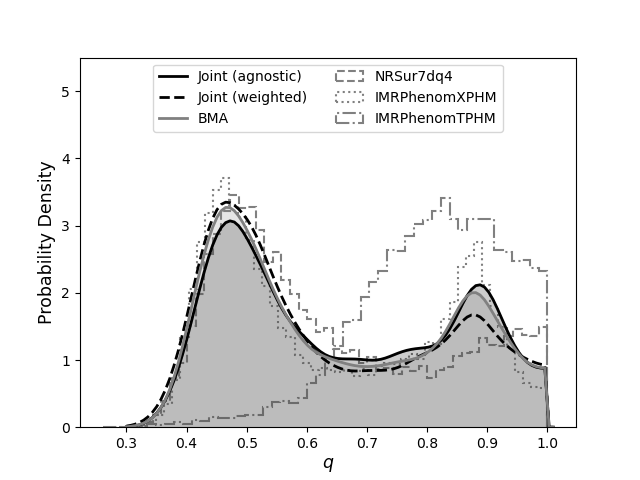
Figure 2: Comparison between the inferred mass ratio $q$, defined as the secondary mass divided by the primary mass and is therefore always $\leq 1$, for GW200129_065458. The Joint posteriors were obtained by performing a single analysis that marginalized over the NRSur7dq4, IMRPhenomXPHM and IMRPhenomTPHM models. The Joint (agnostic) posterior used a uniform prior for the choice of model and the Joint (weighted) posterior used a prior weighted towards the NRSur7dq4 model. The BMA posterior combined posterior distributions obtained with the NRSur7dq4, IMRPhenomXPHM, IMRPhenomTPHM models according to Eq. 3. The JBA was $2.5\times$ faster to compute that the BMA posterior.

Our JBA inferred model probabilities of 0.30, 0.69 and 0.01 for $m_{\mathrm{NRS}}$, $m_{\mathrm{XPHM}}$ and $m_{\mathrm{TPHM}}$ respectively. According to these model probabilities, $m_{\mathrm{XPHM}}$ best describes the data, $m^{*}=m_{\mathrm{XPHM}}$. This is consistent with the inferred model evidences since the BMA combined individual distributions with weights 0.31, 0.68 and 0.01 for $m_{\mathrm{NRS}}$, $m_{\mathrm{XPHM}}$ and $m_{\mathrm{TPHM}}$ models respectively.

Although the JBA marginalizes over multiple models by construction, we can estimate the model-dependent posterior distribution $p(\bm{\lambda}|d,m^{*})$ by selecting only the independent samples with model $m^{*}$. Combined with the ability to accurately and efficiently infer the model probabilities, the JBA can be used to accelerate the inference of $p(\bm{\lambda}|d,m^{*})$.

Fig. 3 compares the model-dependent posterior for the binary’s mass ratio, $p(q|d,m_{i})$, obtained from analysing GW200129 with each model separately and an estimate for $p(q|d,m_{i})$ calculated by selecting only the independent samples obtained from the JBA with model $m_{i}$. In general we see excellent agreement between the two estimates for $p(q|d,m^{*})$. However, we do see a small difference for $p(q|d,m_{\mathrm{TPHM}})$. While insignificant for a BMS analysis (since $m_{\mathrm{TPHM}}$ has the lowest evidence), this is unsurprising since the JBA posterior contains only $\sim 300$ independent samples with $m_{\mathrm{TPHM}}$ compared to $\sim 44,000$ with $m_{\mathrm{XPHM}}$. Of course, this level of agreement can be improved by allowing the sampler to run for longer and therefore collecting a greater number of samples or by simply combining different independent JBA analyses.

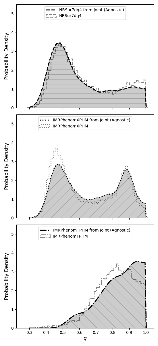
Figure 3: Comparison between the model-dependent posterior for the binaries mass ratio $q$ obtained from analysing GW200129_065458 with each model separately and an estimate for $p(q|d,m_{i})$ calculated by selecting only the independent samples obtained from the Joint (agnostic) analysis with model $m_{i}$.

We have therefore shown that a JBA can infer $p(\bm{\lambda}|d,m_{i})$ and in particular $p(\bm{\lambda}|d,m^{*})$. As demonstrated previously, a significant advantage of performing the JBA is that the JBA is significantly cheaper to perform. We found that the JBA terminated $2.5\times$ faster than the total time required to apply BMS; the JBA took a total of $\sim 4$ hours to complete on 400 CPUs while applying BMS took a total of $\sim 10$ hours to generate on the same number of CPUs: $\sim 4$ hours for $m_{\mathrm{NRS}}$, $\sim 3.5$ hours for $m_{\mathrm{TPHM}}$ and $\sim 2.5$ for $m_{\mathrm{XPHM}}$ models respectively. As discussed, the JBA obtained $\sim 44,000$ samples for $m^{*}$ while BMS selected the posterior with $\sim 60,000$ samples. In general, the JBA obtained $\sim 20,000$, $\sim 44,000$ and $\sim 300$ samples for $m_{\mathrm{NRS}}$, $m_{\mathrm{XPHM}}$ and $m_{\mathrm{TPHM}}$ respectively while the BMA analysis combined $\sim 30,000$, $\sim 60,000$ and $\sim 1000$ samples for $m_{\mathrm{NRS}}$, $m_{\mathrm{XPHM}}$ and $m_{\mathrm{TPHM}}$ respectively. However, the BMA discarded $\sim 90,000$ model-dependent samples, most obtained with $m_{\mathrm{TPHM}}$.

a Subtleties in Bayesian Model Selection

Our analysis of GW200129 concludes that $m_{\mathrm{XPHM}}$ has the largest model probability out of the models considered and therefore it best describes the data. At first glance this seems to be inconsistent with the conclusions presented in Ref. [54] since it was found that $m_{\mathrm{NRS}}$ is the most accurate model in the region of parameter space of GW200129. This highlights an important caveat with using the Bayesian evidence for BMS: the model with the larger evidence will not necessarily be the model that most accurately describes the observed GW.

To demonstrate this, consider the following simulated signal: we simulate a signal with parameters that match the most likely GW found from Ref. [54] with $m_{\mathrm{NRS}}$ and inject it into real GW strain data 2 seconds prior to reported merger time of GW200129 in Hanford, Livingston and Virgo. We then analyse the strain data and marginalize over $m_{\mathrm{NRS}},m_{\mathrm{XPHM}}$ and $m_{\mathrm{TPHM}}$ using the same settings as described above. Since the ensemble of models used in the recovery analysis includes $m_{\mathrm{NRS}}$, there is no systematic bias as we are including the exact model that was used to simulate the injection; in other words, $m_{\mathrm{NRS}}$ is perfectly accurate for describing the simulated GW.

For this specific simulated signal, our JBA concludes that $m_{\mathrm{XPHM}}$ has the greatest support in the data since the model probabilities are 0.38, 0.58 and 0.04 for $m_{\mathrm{NRS}}$, $m_{\mathrm{XPHM}}$ and $m_{\mathrm{TPHM}}$ models respectively. However, if we compare the maximum likelihood estimates from $m_{\mathrm{NRS}}$ and $m_{\mathrm{XPHM}}$, where the maximum likelihood estimate identifies the parameters $\hat{\bm{\lambda}}$ that maximizes the likelihood distribution, we find that $m_{\mathrm{NRS}}$ has the larger maximum likelihood. We ascertain that $m_{\mathrm{XPHM}}$ has the greatest support in the data, of those models considered, since it’s likelihood distribution is more tightly constrained with a slightly larger prior probability.

This simulated signal highlights that although the model probability can be inferred, this probability does not necessarily correlate with the model accuracy, and therefore care must be taken when interpreting the result. One method for mitigating misinterpretation is to use external knowledge of model accuracy to inform the prior for the choice of model.

b Priors

A JBA allows for the user to specify custom priors for the choice of model. This therefore acts as a means of expressing what is already known, or generally agreed upon, regarding the choice of model. One of the problems with using a custom prior is that it must be well motivated.

One option for deriving a custom prior for the choice of model involves generating a weighted Categorical prior, where the weights are correlated with the accuracy of the model, as encoded in the match [see e.g. 78], between each model and a series of numerical relativity simulations in the relevant region of parameter space; a model with a larger match has a larger weight. This works on the principle that the match quantifies how similar a waveform is to a fiducial true waveform: a match of 1 (0) implies that the two waveforms are identical (orthogonal). For example, the weights could be based on the average value of $\log_{10}\,(1-\mathrm{match})^{-1}$, since a model with a poor (good) match to numerical relativity simulations will have a smaller (larger) weight; the weights should be normalized such that the sum is unity. However, averaging the match across a given region of parameter space may not be optimal since models tend to perform differently in different regions of the parameter space. Consequently, a parameter space dependent prior may perform better. We leave a detailed investigation to future work.

In order to demonstrate that a BMS analysis can take into consideration external knowledge of model accuracy, we re-analyse the injection detailed in Sec. a with a weighted Categorical prior for the choice of model. To reflect the fact that $m_{\mathrm{NRS}}$ is the most accurate model, we generated a prior that favours $m_{\mathrm{NRS}}$; for the ease of presentation, we chose weights $0.6,0.3,0.1$ for $m_{\mathrm{NRS}}$, $m_{\mathrm{XPHM}}$ and $m_{\mathrm{TPHM}}$ respectively. We gave $m_{\mathrm{NRS}}$ twice the weight of $m_{\mathrm{XPHM}}$ since $\log_{10}\,(1-\mathrm{match})^{-1}$ is roughly twice as large for $m_{\mathrm{NRS}}$ than $m_{\mathrm{XPHM}}$ in the region of parameter space of the simulated signal. Under this informed prior, the JBA infers model probabilities 0.54, 0.44 and 0.02 for $m_{\mathrm{NRS}}$, $m_{\mathrm{XPHM}}$ and $m_{\mathrm{TPHM}}$ models respectively, which are consistent with simply reweighting the model probabilities obtained under an agnostic prior.

We next use this weighted Categorical prior for a re-analysis of GW200129. In Fig. 2 we see that the JBA with a weighted prior more closely resembles the NRSur7dq4 posterior distribution with less support at $q\sim 0.9$ where only the IMRPhenomXPHM and IMRPhenomTPHM find any substantial probability. Under the weighted prior, we find that $p(m_{\mathrm{NRS}}|d)$ increases from 0.30 to 0.53. This result is therefore now inline with the conclusions presented in Ref. [54].

V Bayes’ factors

When multiple models are available, it is natural to quantify how much one model is preferred to another. Within the Bayesian framework, the primary tool for comparing the performance of two competing models is the Bayes’ factor. The log Bayes’ factor for model $A$ over model $B$ is calculated by simply subtracting the log model evidences: $\log_{10}\mathcal{B}_{AB}=\log_{10}\mathcal{Z}_{A}-\log_{10}\mathcal{Z}_{B}$. A log Bayes’ factor $>0$ indicates a preference for model $A$ over model $B$ and in general, if the log Bayes’ factor is $>1$ there is strong evidence to suggest that model $A$ is preferred to model $B$ [79].

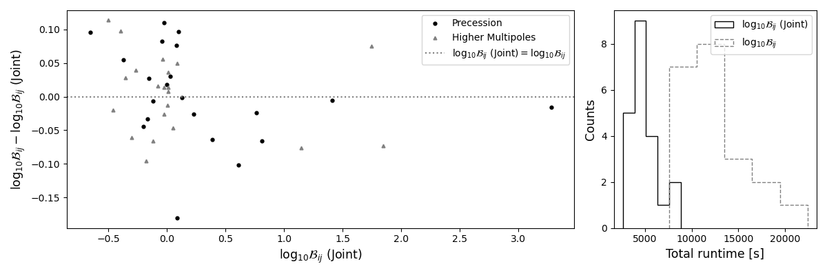
Figure 4: Left: Comparison between the $\log_{10}$ Bayes’ factors obtained from a single JBA that marginalized over the IMRPhenomXAS, IMRPhenomXP and IMRPhenomXHM models, $\log_{10}\mathcal{B}_{ij}\,\,({\mathrm{Joint}})$, and the $\log_{10}$ Bayes’ factors calculated by comparing evidences from 3 separate analyses, an IMRPhenomXAS analysis, IMRPhenomXP analysis and an IMRPhenomXHM analysis, $\log_{10}\mathcal{B}_{ij}$. Right: Histogram showing the total time taken to calculate $\log_{10}\mathcal{B}_{ij}\,\,({\mathrm{Joint}})$ and $\log_{10}\mathcal{B}_{ij}$ shown in the Left panel.

Since the log Bayes’ factor requires estimates for the model’s evidence $\mathcal{Z}_{i}$, this requires running multiple parameter estimation analyses, one for each of the models $A$ and $B$, which is computationally expensive. However, as described in Section 5 of Ref. [68], the log Bayes’ factor can be approximated by running a single JBA that marginalizes over models $A$ and $B$. Here, the ratio of inferred model probabilities $p(m_{A}|d)/p(m_{B}|d)=\mathcal{N}_{A}/\mathcal{N}_{B}$ (see Eq. 5) gives the posterior odds for model $A$ over model $B$. For the case of uniform priors for the choice of model, the posterior odds is equivalent to the Bayes’ factor,

$$\begin{split}\log_{10}\mathcal{B}_{AB}&=\log_{10}\mathcal{Z}_{A}-\log_{10}\mathcal{Z}_{B}\\ &\approx\log_{10}\mathcal{N}_{A}-\log_{10}\mathcal{N}_{B}.\end{split}$$ (7)

If we wish to calculate two log Bayes’ factors simultaneously, for example comparing model $A$ to model $B$ and model $A$ to model $C$, we can simply perform a single analysis that marginalizes over all 3 models $A$, $B$ and $C$ while assuming uniform priors for the choice of model, rather than launching 3 separate parameter estimation analyses to calculate $\mathcal{Z}_{A},\mathcal{Z}_{B},\mathcal{Z}_{C}$. As demonstrated in Secs. III and  IV, this has the potential to greatly reduce the computational cost of calculating the Bayes’ factor.

In order to show that the JBA can greatly reduce the computational cost of calculating the log Bayes’ factor while still maintaining accuracy, we calculated two log Bayes’ factors from a single JBA and compared the results to the log Bayes’ factors estimated from 3 separate analyses. Owing to the computational cost of generating 2 log Bayes’ factors, we only considered the first 20 randomly chosen binaries described in Sec. III. Unlike in Sec. III, we simulated the injected GWs with a complete model (IMRPhenomXPHM [44]). Our recovery analysis marginalized over an aligned-spin (IMRPhenomXAS [42]), precessing (IMRPhenomXP) and higher-order multipole (IMRPhenomXHM [43]) models.

Since a precessing model includes all 6 spin degrees of freedom, it analyses a 15-dimensional parameter space, see Sec. III for details. In comparison, an aligned-spin model restricts spins to be aligned with the orbital angular momentum, meaning that only 2 spin degrees of freedom are probed. Consequently an aligned-spin model analyses an 11-dimensional parameter space. The log Bayes’ factor in favour of the precessing model over the aligned-spin model therefore quantifies the support for spins misaligned with the orbital angular momentum. This log Bayes’ factor can therefore be interpreted as a measure for the evidence of spin-induced orbital precession in the observed GW [80]. Similarly, a higher-order multipole model includes higher order multipoles but restricts spins to be aligned with the orbital angular momentum. By calculating the log Bayes’ factor in favour of the higher-order multipole model over the aligned-spin model, we quantify the evidence for higher order multipoles in the observed GW.

Our JBA must therefore sample a 15-dimensional parameter space for the precessing model and an 11-dimensional parameter space for both the higher-order multipole and aligned-spin models. Since the aligned-spin parameter space is simply a subspace of the full precessing parameter space, we accomplish this transition by always sampling the 15-dimension parameter space and simply projecting $\tilde{\bm{\lambda}}$ onto the aligned-spin parameter space when an aligned-spin model is chosen during the sampling.

The left panel of Fig. 4 compares the log Bayes’ factors in favour of precession and higher order multipoles calculated from a single JBA to the log Bayes’ factors estimated from 3 separate analyses. In general we see that the difference in log Bayes’ factors are $\lesssim 0.1$ with the largest differences occurring for systems with $\log_{10}\mathcal{B}_{ij}\sim 0$. This level of disagreement is consistent with the expected error in the estimated log Bayes’ factor from the pBilby parameter estimation software and the IMRPhenomX waveform family, see e.g. Table IV in Ref. [88]. We also note that in previous LVK analyses, when $\log_{10}\mathcal{B}_{ij}\sim 0$, the Bayes’ factor is not quoted and therefore the difference in $\log_{10}\mathcal{B}_{ij}$ between the two methods is insignificant.

Importantly, we also see that the Bayes’ factors are consistent not only for cases where there is very little evidence for precession and/or higher order multipoles ($\sim 0$) but also cases where there is very strong evidence for precession and/or higher order multipoles ($\sim 3.0$). This shows that a JBA can be used to estimate the log Bayes’ factor for all signals reported by the LVK to date [4, 5, 53]. This technique is likely also accurate for signals displaying greater evidence for precession and/or higher order multipoles than $\sim 3.0$ but this region was not explored in our analysis since our binaries were randomly chosen.

The right panel of Fig. 4 shows the total runtime for computing 40 log Bayes’ factors (2 log Bayes’ factors for each injection) from a single JBA to the log Bayes’ factors estimated from 3 separate analyses. We see that the JBA computed comparable log Bayes’ factors on average $2.6\times$ faster than by comparing model evidences. This demonstrates that not only can the JBA maintain accuracy in the computation of the log Bayes’ factor, but it can greatly reduce the computational cost.

VI Discussion

In this work we simultaneously inferred the model and model properties in a joint Bayesian analysis. Although JBAs has already been used both inside [see e.g. 68] and outside [see e.g. 69] of GW research, we demonstrated that it can be used to address waveform systematics in BBH mergers while also offering a computationally cheaper solution compared to applying BMA.

We validated this JBA by analysing GWs emitted from 100 randomly chosen binaries where we marginalized over three of the latest GW models. Although our simulated signals had SNRs ranging between 3.0 and 47.0, all of the posterior distributions obtained with the JBA were consistent with those obtained using BMA. In fact, 98% of the posterior distributions were statistically identical between the two approaches. Remarkably, this method marginalizes over three models on average $2.5\times$ faster than simply applying BMA. As a real world example, we also applied the JBA to analyse GW200129_065458 and investigated how custom priors for the choice of model can be used to reflect our knowledge of model accuracy. We then demonstrated that the model with the largest evidence does not necessarily correlate with the model accuracy and therefore care must be taken when interpreting $p(m|d)$.

This alternative method of marginalizing over a set of models can also be used to significantly reduce the computational cost of computing one or more Bayes’ factors. For example, we demonstrated that the Bayes’ factor in favour of precession and higher order multipoles can be generated from a single analysis and not only do we obtain comparable Bayes’ factors, but we generate them on average $2.6\times$ faster compared to conventional methods.

The method presented in this work is timely since the fourth gravitational-wave observing run, where $\sim 200$ GW signals are likely to be observed, is scheduled to commence early next year. During this observing run we are likely to observe a significant number of events that lie in extreme regions of the parameter space, where it will be desirable to marginalize over the latest waveform models in order to take into consideration model systematics. The method presented in this work provides a simple, robust and computationally efficient way to marginalize over multiple models.

VII Acknowledgements

We are grateful to Gregory Ashton, Stephen Fairhurst, Mark Hannam, Soichiro Morisaki, Vivien Raymond and Jonathan Thompson for comments on this manuscript as well as Mark Hannam for continued discussions throughout this project. This work was supported by European Research Council (ERC) Consolidator Grant 647839. All calculations were performed using the supercomputing facilities at Cardiff University operated by Advanced Research Computing at Cardiff (ARCCA) on behalf of the Cardiff Supercomputing Facility and the HPC Wales and Supercomputing Wales (SCW) projects. The computational resources at Cardiff University are part-funded by the European Regional Development Fund (ERDF) via the Welsh Government and STFC grant ST/I006285/1. This research made use of data, software and/or web tools obtained from the Gravitational Wave Open Science Center (https://www.gw-openscience.org), a service of LIGO Laboratory, the LIGO Scientific Collaboration and the Virgo Collaboration. LIGO is funded by the U.S. National Science Foundation. Virgo is funded by the French Centre National de Recherche Scientifique (CNRS), the Italian Istituto Nazionale della Fisica Nucleare (INFN) and the Dutch Nikhef, with contributions by Polish and Hungarian institutes. This material is based upon work supported by NSF’s LIGO Laboratory which is a major facility fully funded by the National Science Foundation.

Plots were prepared with Matplotlib [89], PESummary [90] and Bilby [13]. Parameter estimation was performed with the pBilby parameter estimation software [15], which made use of the dynesty nesting sampling package [70]. NumPy [91] and Scipy [92] were also used during our analysis.

Appendix A Percentile-Percentile test

We show the posterior distributions obtained by the JBA described in Section III in the form of a percentile-percentile (P-P) plot in Fig. 5. A P-P plot is useful for identifying biases in the inferred posterior distributions since it plots the fraction of signals with the injected binary lying within a given credible interval against the given credible interval. If the posterior distributions are biased, we would expect to see that the $x\%$ credible interval contains the injected binary more or less than $x\%$ of the time. To quantify the level of bias, we calculate p-values in each dimension, by performing a Kolmogorov-Smirnov (KS) test [93, 94] against the expected uniform distribution, and a combined p-value, by combining the individual p-values using Fisher’s method.

As can be seen in Fig. 5, the majority of dimensions show no bias since they are consistent with a uniform distribution at $>5\%$ confidence. Although the primary spin magnitude $a_{1}$ and coalescence time $t_{c}$ show a small bias (p-values $<0.05$) and the combined p-value shows an overall bias in the inferred distributions: $0.01$, this is unsurprising since the P-P test is only expected to show no bias when the model used to generate the simulated signals exactly matches the model used for recovery [59]. Since we have marginalized over multiple models, each with different inherent assumptions, we have introduced additional uncertainty in the data analysis.

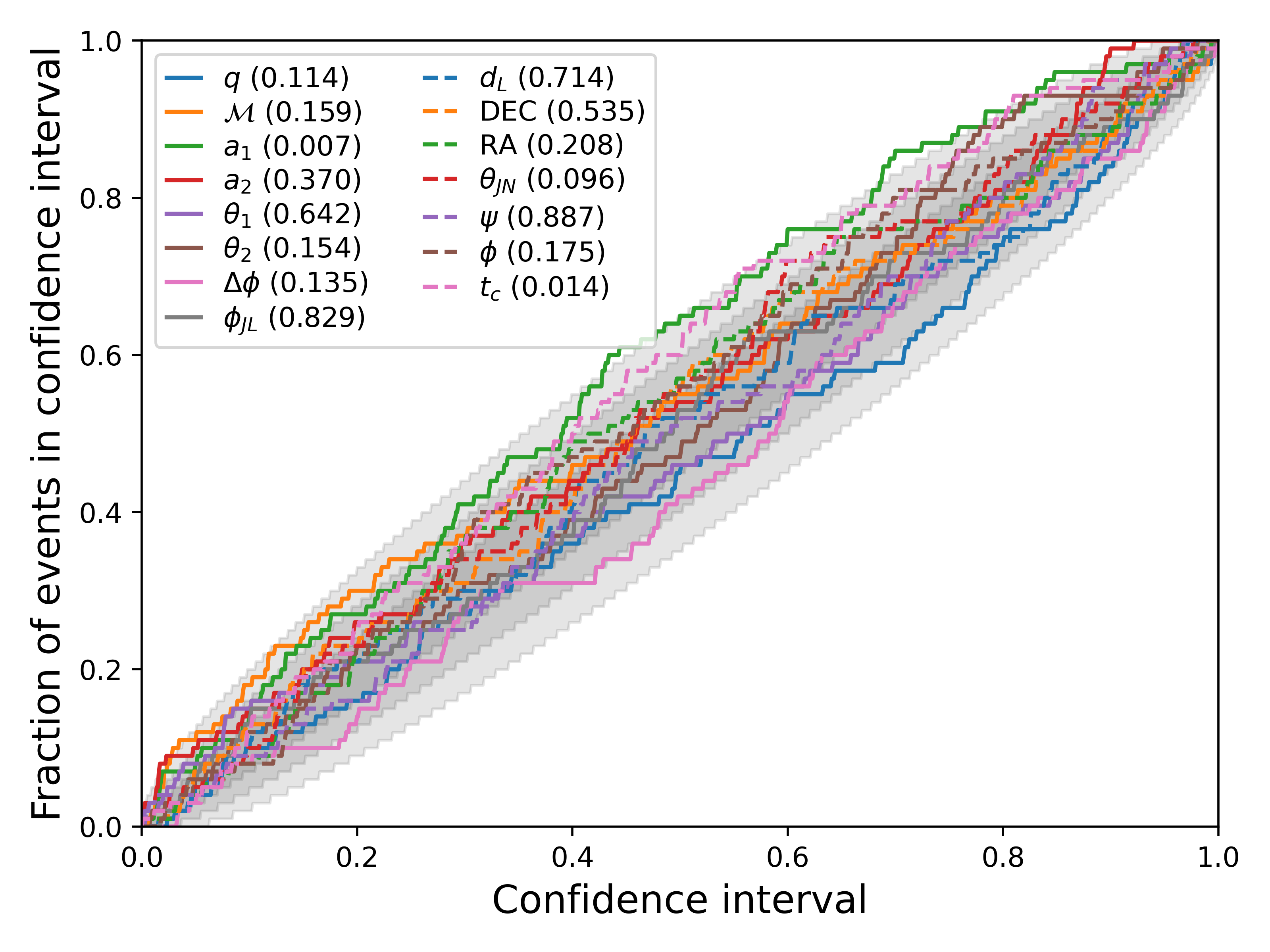
Figure 5: Posterior distributions obtained when analysing 100 randomly chosen binaries modelled with the IMRPhenomXP [44] model. The grey regions show the cumulative $1\sigma$, $2\sigma$ and $3\sigma$ confidence intervals expected from a uniform distribution, which is expected if the results are unbiased. Each line shows the cumulative fraction of events within the confidence interval for a given parameter. The posterior distributions were obtained by marginalizing over the IMRPhenomXP, IMRPhenomTP [45] and IMRPhenomPv3 [38] models according to Eq. 5. The numbers in the legend show the Kolmogorov-Smirnov p-value [93, 94] when comparing each line to the expected uniform distribution.

We also generated a P-P plot showing the posterior distributions obtained by the BMA analysis also described in Section III. As expected, we saw excellent agreement between the JBA and BMA P-P plots. To quantify the level of agreement, we generated individual p-values for each dimension by performing a KS test between comparable lines on the two P-P plots and combined them using Fisher’s method. We find a combined p-value of $0.47$, which highlights that there is no statistical difference between P-P plots.

References

- [1] B. P. Abbott et al. Observation of Gravitational Waves from a Binary Black Hole Merger. Phys. Rev. Lett., 116(6):061102, 2016.
- [2] J. Aasi et al. Advanced LIGO. Class. Quant. Grav., 32:074001, 2015.
- [3] F Acernese, M Agathos, K Agatsuma, D Aisa, N Allemandou, A Allocca, J Amarni, P Astone, G Balestri, G Ballardin, et al. Advanced virgo: a second-generation interferometric gravitational wave detector. Classical and Quantum Gravity, 32(2):024001, 2014.
- [4] B. P. Abbott et al. GWTC-1: A Gravitational-Wave Transient Catalog of Compact Binary Mergers Observed by LIGO and Virgo during the First and Second Observing Runs. Phys. Rev. X, 9(3):031040, 2019.
- [5] R. Abbott et al. GWTC-2: Compact Binary Coalescences Observed by LIGO and Virgo During the First Half of the Third Observing Run. Phys. Rev. X, 11:021053, 2021.
- [6] R. Abbott et al. GWTC-2.1: Deep Extended Catalog of Compact Binary Coalescences Observed by LIGO and Virgo During the First Half of the Third Observing Run. 8 2021.
- [7] Alexander H Nitz, Thomas Dent, Gareth S Davies, Sumit Kumar, Collin D Capano, Ian Harry, Simone Mozzon, Laura Nuttall, Andrew Lundgren, and Márton Tápai. 2-ogc: Open gravitational-wave catalog of binary mergers from analysis of public advanced ligo and virgo data. The Astrophysical Journal, 891(2):123, 2020.
- [8] Tejaswi Venumadhav, Barak Zackay, Javier Roulet, Liang Dai, and Matias Zaldarriaga. New binary black hole mergers in the second observing run of advanced ligo and advanced virgo. Physical Review D, 101(8):083030, 2020.
- [9] Barak Zackay, Tejaswi Venumadhav, Liang Dai, Javier Roulet, and Matias Zaldarriaga. Highly spinning and aligned binary black hole merger in the advanced ligo first observing run. Physical Review D, 100(2):023007, 2019.
- [10] Barak Zackay, Liang Dai, Tejaswi Venumadhav, Javier Roulet, and Matias Zaldarriaga. Detecting gravitational waves with disparate detector responses: two new binary black hole mergers. arXiv preprint arXiv:1910.09528, 2019.
- [11] Alexander H. Nitz, Collin D. Capano, Sumit Kumar, Yi-Fan Wang, Shilpa Kastha, Marlin Schäfer, Rahul Dhurkunde, and Miriam Cabero. 3-OGC: Catalog of Gravitational Waves from Compact-binary Mergers. Astrophys. J., 922(1):76, 2021.
- [12] C. Pankow, P. Brady, E. Ochsner, and R. O’Shaughnessy. Novel scheme for rapid parallel parameter estimation of gravitational waves from compact binary coalescences. Phys. Rev. D, 92(2):023002, 2015.
- [13] Gregory Ashton et al. BILBY: A user-friendly Bayesian inference library for gravitational-wave astronomy. Astrophys. J. Suppl., 241(2):27, 2019.
- [14] I. M. Romero-Shaw et al. Bayesian inference for compact binary coalescences with bilby: validation and application to the first LIGO–Virgo gravitational-wave transient catalogue. Mon. Not. Roy. Astron. Soc., 499(3):3295–3319, 2020.
- [15] Rory J. E. Smith, Gregory Ashton, Avi Vajpeyi, and Colm Talbot. Massively parallel Bayesian inference for transient gravitational-wave astronomy. Mon. Not. Roy. Astron. Soc., 498(3):4492–4502, 2020.
- [16] C. M. Biwer, Collin D. Capano, Soumi De, Miriam Cabero, Duncan A. Brown, Alexander H. Nitz, and V. Raymond. PyCBC Inference: A Python-based parameter estimation toolkit for compact binary coalescence signals. Publ. Astron. Soc. Pac., 131(996):024503, 2019.
- [17] Jacob Lange, Richard O’Shaughnessy, and Monica Rizzo. Rapid and accurate parameter inference for coalescing, precessing compact binaries. 5 2018.
- [18] J. Veitch et al. Parameter estimation for compact binaries with ground-based gravitational-wave observations using the LALInference software library. Phys. Rev. D, 91(4):042003, 2015.
- [19] Michael J. Williams, John Veitch, and Chris Messenger. Nested sampling with normalizing flows for gravitational-wave inference. Phys. Rev. D, 103(10):103006, 2021.
- [20] Hunter Gabbard, Chris Messenger, Ik Siong Heng, Francesco Tonolini, and Roderick Murray-Smith. Bayesian parameter estimation using conditional variational autoencoders for gravitational-wave astronomy. Nature Phys., 18(1):112–117, 2022.
- [21] Stephen R. Green and Jonathan Gair. Complete parameter inference for GW150914 using deep learning. Mach. Learn. Sci. Tech., 2(3):03LT01, 2021.
- [22] Barak Zackay, Liang Dai, and Tejaswi Venumadhav. Relative Binning and Fast Likelihood Evaluation for Gravitational Wave Parameter Estimation. 6 2018.
- [23] Nathaniel Leslie, Liang Dai, and Geraint Pratten. Mode-by-mode relative binning: Fast likelihood estimation for gravitational waveforms with spin-orbit precession and multiple harmonics. Phys. Rev. D, 104(12):123030, 2021.
- [24] Leo P. Singer and Larry R. Price. Rapid Bayesian position reconstruction for gravitational-wave transients. Phys. Rev. D, 93(2):024013, 2016.
- [25] Neil J. Cornish. Rapid and Robust Parameter Inference for Binary Mergers. Phys. Rev. D, 103(10):104057, 2021.
- [26] Nicholas Metropolis and Stanislaw Ulam. The monte carlo method. Journal of the American statistical association, 44(247):335–341, 1949.
- [27] John Skilling. Nested sampling for general Bayesian computation. Bayesian Analysis, 1(4):833–859, 2006.
- [28] Alejandro Bohé et al. Improved effective-one-body model of spinning, nonprecessing binary black holes for the era of gravitational-wave astrophysics with advanced detectors. Phys. Rev. D, 95(4):044028, 2017.
- [29] Roberto Cotesta, Alessandra Buonanno, Alejandro Bohé, Andrea Taracchini, Ian Hinder, and Serguei Ossokine. Enriching the Symphony of Gravitational Waves from Binary Black Holes by Tuning Higher Harmonics. Phys. Rev. D, 98(8):084028, 2018.
- [30] Roberto Cotesta, Sylvain Marsat, and Michael Pürrer. Frequency domain reduced order model of aligned-spin effective-one-body waveforms with higher-order modes. Phys. Rev. D, 101(12):124040, 2020.
- [31] Serguei Ossokine et al. Multipolar Effective-One-Body Waveforms for Precessing Binary Black Holes: Construction and Validation. Phys. Rev. D, 102(4):044055, 2020.
- [32] Stanislav Babak, Andrea Taracchini, and Alessandra Buonanno. Validating the effective-one-body model of spinning, precessing binary black holes against numerical relativity. Phys. Rev. D, 95(2):024010, 2017.
- [33] Yi Pan, Alessandra Buonanno, Andrea Taracchini, Lawrence E. Kidder, Abdul H. Mroué, Harald P. Pfeiffer, Mark A. Scheel, and Béla Szilágyi. Inspiral-merger-ringdown waveforms of spinning, precessing black-hole binaries in the effective-one-body formalism. Phys. Rev. D, 89(8):084006, 2014.
- [34] Sascha Husa, Sebastian Khan, Mark Hannam, Michael Pürrer, Frank Ohme, Xisco Jiménez Forteza, and Alejandro Bohé. Frequency-domain gravitational waves from nonprecessing black-hole binaries. I. New numerical waveforms and anatomy of the signal. Phys. Rev. D, 93(4):044006, 2016.
- [35] Sebastian Khan, Sascha Husa, Mark Hannam, Frank Ohme, Michael Pürrer, Xisco Jiménez Forteza, and Alejandro Bohé. Frequency-domain gravitational waves from nonprecessing black-hole binaries. II. A phenomenological model for the advanced detector era. Phys. Rev. D, 93(4):044007, 2016.
- [36] Lionel London, Sebastian Khan, Edward Fauchon-Jones, Cecilio García, Mark Hannam, Sascha Husa, Xisco Jiménez-Forteza, Chinmay Kalaghatgi, Frank Ohme, and Francesco Pannarale. First higher-multipole model of gravitational waves from spinning and coalescing black-hole binaries. Phys. Rev. Lett., 120(16):161102, 2018.
- [37] Mark Hannam, Patricia Schmidt, Alejandro Bohé, Leïla Haegel, Sascha Husa, Frank Ohme, Geraint Pratten, and Michael Pürrer. Simple Model of Complete Precessing Black-Hole-Binary Gravitational Waveforms. Phys. Rev. Lett., 113(15):151101, 2014.
- [38] Sebastian Khan, Katerina Chatziioannou, Mark Hannam, and Frank Ohme. Phenomenological model for the gravitational-wave signal from precessing binary black holes with two-spin effects. Phys. Rev. D, 100(2):024059, 2019.
- [39] Sebastian Khan, Frank Ohme, Katerina Chatziioannou, and Mark Hannam. Including higher order multipoles in gravitational-wave models for precessing binary black holes. Phys. Rev. D, 101(2):024056, 2020.
- [40] Vijay Varma, Scott E. Field, Mark A. Scheel, Jonathan Blackman, Davide Gerosa, Leo C. Stein, Lawrence E. Kidder, and Harald P. Pfeiffer. Surrogate models for precessing binary black hole simulations with unequal masses. Phys. Rev. Research., 1:033015, 2019.
- [41] Vijay Varma, Scott E. Field, Mark A. Scheel, Jonathan Blackman, Lawrence E. Kidder, and Harald P. Pfeiffer. Surrogate model of hybridized numerical relativity binary black hole waveforms. Phys. Rev. D, 99(6):064045, 2019.
- [42] Geraint Pratten, Sascha Husa, Cecilio Garcia-Quiros, Marta Colleoni, Antoni Ramos-Buades, Hector Estelles, and Rafel Jaume. Setting the cornerstone for a family of models for gravitational waves from compact binaries: The dominant harmonic for nonprecessing quasicircular black holes. Phys. Rev. D, 102(6):064001, 2020.
- [43] Cecilio García-Quirós, Marta Colleoni, Sascha Husa, Héctor Estellés, Geraint Pratten, Antoni Ramos-Buades, Maite Mateu-Lucena, and Rafel Jaume. Multimode frequency-domain model for the gravitational wave signal from nonprecessing black-hole binaries. Phys. Rev. D, 102(6):064002, 2020.
- [44] Geraint Pratten et al. Computationally efficient models for the dominant and subdominant harmonic modes of precessing binary black holes. Phys. Rev. D, 103(10):104056, 2021.
- [45] Héctor Estellés, Antoni Ramos-Buades, Sascha Husa, Cecilio García-Quirós, Marta Colleoni, Leïla Haegel, and Rafel Jaume. Phenomenological time domain model for dominant quadrupole gravitational wave signal of coalescing binary black holes. Phys. Rev. D, 103(12):124060, 2021.
- [46] Héctor Estellés, Sascha Husa, Marta Colleoni, David Keitel, Maite Mateu-Lucena, Cecilio García-Quirós, Antoni Ramos-Buades, and Angela Borchers. Time-domain phenomenological model of gravitational-wave subdominant harmonics for quasicircular nonprecessing binary black hole coalescences. Phys. Rev. D, 105(8):084039, 2022.
- [47] Héctor Estellés, Marta Colleoni, Cecilio García-Quirós, Sascha Husa, David Keitel, Maite Mateu-Lucena, Maria de Lluc Planas, and Antoni Ramos-Buades. New twists in compact binary waveform modeling: A fast time-domain model for precession. Phys. Rev. D, 105(8):084040, 2022.
- [48] Chinmay Kalaghatgi, Mark Hannam, and Vivien Raymond. Parameter estimation with a spinning multimode waveform model. Phys. Rev. D, 101(10):103004, 2020.
- [49] Feroz H. Shaik, Jacob Lange, Scott E. Field, Richard O’Shaughnessy, Vijay Varma, Lawrence E. Kidder, Harald P. Pfeiffer, and Daniel Wysocki. Impact of subdominant modes on the interpretation of gravitational-wave signals from heavy binary black hole systems. Phys. Rev. D, 101(12):124054, 2020.
- [50] R. Abbott et al. Properties and Astrophysical Implications of the 150 M⊙ Binary Black Hole Merger GW190521. Astrophys. J. Lett., 900(1):L13, 2020.
- [51] R. Abbott et al. GW190412: Observation of a Binary-Black-Hole Coalescence with Asymmetric Masses. Phys. Rev. D, 102(4):043015, 2020.
- [52] R. Abbott et al. GW190814: Gravitational Waves from the Coalescence of a 23 Solar Mass Black Hole with a 2.6 Solar Mass Compact Object. Astrophys. J. Lett., 896(2):L44, 2020.
- [53] R. Abbott et al. GWTC-3: Compact Binary Coalescences Observed by LIGO and Virgo During the Second Part of the Third Observing Run. 11 2021.
- [54] Mark Hannam, Charlie Hoy, Jonathan E. Thompson, Stephen Fairhurst, Vivien Raymond, and members of the LIGO, Virgo collaboration. Measurement of general-relativistic precession in a black-hole binary. 12 2021.
- [55] Michael Pürrer and Carl-Johan Haster. Gravitational waveform accuracy requirements for future ground-based detectors. Phys. Rev. Res., 2(2):023151, 2020.
- [56] Christopher J. Moore, Eliot Finch, Riccardo Buscicchio, and Davide Gerosa. Testing general relativity with gravitational-wave catalogs: the insidious nature of waveform systematics. 3 2021.
- [57] Eleanor Hamilton, Lionel London, Jonathan E. Thompson, Edward Fauchon-Jones, Mark Hannam, Chinmay Kalaghatgi, Sebastian Khan, Francesco Pannarale, and Alex Vano-Vinuales. Model of gravitational waves from precessing black-hole binaries through merger and ringdown. Phys. Rev. D, 104(12):124027, 2021.
- [58] Christopher P.L. Berry et al. Quoting parameter-estimation results. Technical Report LIGO-T1500597, 2015.
- [59] Gregory Ashton and Sebastian Khan. Multiwaveform inference of gravitational waves. Phys. Rev. D, 101(6):064037, 2020.
- [60] Tiago M Fragoso, Wesley Bertoli, and Francisco Louzada. Bayesian model averaging: A systematic review and conceptual classification. International Statistical Review, 86(1):1–28, 2018.
- [61] Bertrand Clarke. Comparing bayes model averaging and stacking when model approximation error cannot be ignored. Journal of Machine Learning Research, 4(Oct):683–712, 2003.
- [62] A. Z. Jan, A. B. Yelikar, J. Lange, and R. O’Shaughnessy. Assessing and marginalizing over compact binary coalescence waveform systematics with RIFT. Phys. Rev. D, 102(12):124069, 2020.
- [63] D. Wysocki, R. O’Shaughnessy, Jacob Lange, and Yao-Lung L. Fang. Accelerating parameter inference with graphics processing units. Phys. Rev. D, 99(8):084026, 2019.
- [64] Peter J. Green. Reversible jump Markov chain Monte Carlo computation and Bayesian model determination. Biometrika, 82(4):711–732, 1995.
- [65] Neil J. Cornish and Tyson B. Littenberg. Tests of Bayesian Model Selection Techniques for Gravitational Wave Astronomy. Phys. Rev. D, 76:083006, 2007.
- [66] Neil J. Cornish and Tyson B. Littenberg. BayesWave: Bayesian Inference for Gravitational Wave Bursts and Instrument Glitches. Class. Quant. Grav., 32(13):135012, 2015.
- [67] Tyson B. Littenberg and Neil J. Cornish. Bayesian inference for spectral estimation of gravitational wave detector noise. Phys. Rev. D, 91(8):084034, 2015.
- [68] Gregory Ashton and Tim Dietrich. Understanding binary neutron star collisions with hypermodels. Nature Astron., 07 2022.
- [69] Christophe Andrieu and Arnaud Doucet. Joint bayesian model selection and estimation of noisy sinusoids via reversible jump mcmc. IEEE Transactions on Signal Processing, 47(10):2667–2676, 1999.
- [70] Joshua S. Speagle. dynesty: a dynamic nested sampling package for estimating Bayesian posteriors and evidences. Mon. Not. Roy. Astron. Soc., 493(3):3132–3158, 2020.
- [71] K. S. Thorne. Multipole Expansions of Gravitational Radiation. Rev. Mod. Phys., 52:299–339, 1980.
- [72] J. Lin. Divergence measures based on the shannon entropy. IEEE Transactions on Information Theory, 37(1):145–151, Jan 1991.
- [73] A. Buonanno and T. Damour. Effective one-body approach to general relativistic two-body dynamics. Phys. Rev. D, 59:084006, 1999.
- [74] Parameswaran Ajith et al. Phenomenological template family for black-hole coalescence waveforms. Class. Quant. Grav., 24:S689–S700, 2007.
- [75] Scott E. Field, Chad R. Galley, Jan S. Hesthaven, Jason Kaye, and Manuel Tiglio. Fast prediction and evaluation of gravitational waveforms using surrogate models. Phys. Rev. X, 4(3):031006, 2014.
- [76] Qian Hu and John Veitch. Assessing the model waveform accuracy of gravitational waves. 5 2022.
- [77] Bhooshan Gadre, Michael Pürrer, Scott E. Field, Serguei Ossokine, and Vijay Varma. A fully precessing higher-mode surrogate model of effective-one-body waveforms. 3 2022.
- [78] Benjamin J. Owen. Search templates for gravitational waves from inspiraling binaries: Choice of template spacing. Phys. Rev. D, 53:6749–6761, 1996.
- [79] Robert E. Kass and Adrian E. Raftery. Bayes factors. Journal of the American Statistical Association, 90(430):773–795, 1995.
- [80] Theocharis A. Apostolatos, Curt Cutler, Gerald J. Sussman, and Kip S. Thorne. Spin induced orbital precession and its modulation of the gravitational wave forms from merging binaries. Phys. Rev. D, 49:6274–6297, 1994.
- [81] Stephen Fairhurst, Rhys Green, Mark Hannam, and Charlie Hoy. When will we observe binary black holes precessing? Phys. Rev. D, 102(4):041302, 2020.
- [82] Stephen Fairhurst, Rhys Green, Charlie Hoy, Mark Hannam, and Alistair Muir. Two-harmonic approximation for gravitational waveforms from precessing binaries. Phys. Rev. D, 102(2):024055, 2020.
- [83] Rhys Green, Charlie Hoy, Stephen Fairhurst, Mark Hannam, Francesco Pannarale, and Cory Thomas. Identifying when Precession can be Measured in Gravitational Waveforms. Phys. Rev. D, 103(12):124023, 2021.
- [84] Charlie Hoy, Cameron Mills, and Stephen Fairhurst. Evidence for subdominant multipole moments and precession in merging black-hole-binaries from GWTC-2.1. Phys. Rev. D, 106(2):023019, 2022.
- [85] Soumen Roy, Anand S. Sengupta, and K. G. Arun. Unveiling the spectrum of inspiralling binary black holes. Phys. Rev. D, 103(6):064012, 2021.
- [86] S. Klimenko et al. Method for detection and reconstruction of gravitational wave transients with networks of advanced detectors. Phys. Rev. D, 93(4):042004, 2016.
- [87] Cameron Mills and Stephen Fairhurst. Measuring gravitational-wave higher-order multipoles. Phys. Rev. D, 103(2):024042, 2021.
- [88] Marta Colleoni, Maite Mateu-Lucena, Héctor Estellés, Cecilio García-Quirós, David Keitel, Geraint Pratten, Antoni Ramos-Buades, and Sascha Husa. Towards the routine use of subdominant harmonics in gravitational-wave inference: Reanalysis of GW190412 with generation X waveform models. Phys. Rev. D, 103(2):024029, 2021.
- [89] J. D. Hunter. Matplotlib: A 2D Graphics Environment. CSE, 9:90–95, May 2007.
- [90] Charlie Hoy and Vivien Raymond. PESummary: the code agnostic Parameter Estimation Summary page builder. SoftwareX, 15:100765, 2021.
- [91] Oliphant Travis E. a guide to numpy, 2006.
- [92] Wes McKinney. Data structures for statistical computing in python. In Stéfan van der Walt and Jarrod Millman, editors, Proceedings of the 9th Python in Science Conference, pages 51 – 56, 2010.
- [93] Andrey Kolmogorov. Sulla determinazione empirica di una lgge di distribuzione. Inst. Ital. Attuari, Giorn., 4:83–91, 1933.
- [94] Nickolay Smirnov. Table for estimating the goodness of fit of empirical distributions. The annals of mathematical statistics, 19(2):279–281, 1948.