Robust Rayleigh Regression Method for SAR Image Processing in Presence of Outliers

The presence of outliers (anomalous values) in synthetic aperture radar (SAR) data and the misspecification in statistical image models may result in inaccurate inferences. To avoid such issues, the Rayleigh regression model based on a robust estimation process is proposed as a more realistic approach to model this type of data. This paper aims at obtaining Rayleigh regression model parameter estimators robust to the presence of outliers. The proposed approach considered the weighted maximum likelihood method and was submitted to numerical experiments using simulated and measured SAR images. Monte Carlo simulations were employed for the numerical assessment of the proposed robust estimator performance in finite signal lengths, their sensitivity to outliers, and the breakdown point. For instance, the non-robust estimators show a relative bias value $65$-fold larger than the results provided by the robust approach in corrupted signals. In terms of sensitivity analysis and break down point, the robust scheme resulted in a reduction of about $96\%$ and $10\%$, respectively, in the mean absolute value of both measures, in compassion to the non-robust estimators. Moreover, two SAR data sets were used to compare the ground type and anomaly detection results of the proposed robust scheme with competing methods in the literature.

Keywords
Outliers, Rayleigh regression model, Robust estimation, SAR images

Synthetic aperture radar (SAR) data plays an important role in remote sensing applications [27] due to its capability of providing (i) wide terrain coverage in a short observation of time and (ii) suitable visual information acquisition, independent of weather and illumination conditions [24]. However, SAR images are frequently contaminated by a percentage of outliers (anomalous values)—image pixels that differ significantly from their neighborhood [16]—, which can be related to human-made objects or highly reflective areas [8]. Because such observations do not follow the general behavior of the neighborhood or the observed scene [24], the use of suitable approaches to deal with outliers should be considered to avoid unreliable results in remote sensing applications [8]. For example, in [28], the median was employed to obtain a ground scene predicted (GSP) image based on an image stack of the CARABAS II data set [21]. The resulted image was applied as a reference image in a change detection algorithm. The median is a robust method and was considered in the CARABAS II SAR image data set to remove outliers (military vehicles), resulting in high probability detection values, associated with low false alarm rates, highlighting the importance of robust methods to deal with outliers.

Typical tasks in SAR data analysis and processing include (i) image modeling [7, 36], (ii) identification and classification of distinct ground type [38, 19], and (iii) change detection [25, 45]. The use of statistical models—commonly employed to describe image pixels by a small number of parameters [1]—can generate accurate results for the above SAR-related challenges, as presented in [26] and [42]. The statistical inference methods widely considered for signal and image modeling usually suppose (i) Gaussian or symmetric data [1, 47] and (ii) least-squares or maximum likelihood approaches [1].

However, magnitude SAR image pixels generally present non-Gaussian properties, such as asymmetrical distributions and strictly positive values [27]. These characteristics motivated the proposition of a regression model based on the Rayleigh distribution for SAR image modeling [29]. The Rayleigh regression model is suitable for non-Gaussian situations, where the observed output signal is asymmetric and measured continuously on the real positives values, such as SAR amplitude image pixels. The Rayleigh regression model assumes that the Rayleigh distributed signal mean follows a regression structure involving covariates, unknown parameters, and a link function. In [29], an inference approach for the model parameters, diagnostic tools, asymptotic proprieties of the parameter estimators, and a ground type detector were discussed. Additionally, as in other classes of non-Gaussian regression models, such as the generalized linear model [23], the Rayleigh regression model was derived considering the maximum likelihood approach to estimate its parameters. However, robust tools were not discussed.

The maximum likelihood inference method is asymptotically efficient but lacks robustness against model misspecification and outliers [13, 47]. On the other hand, robust approaches are not significantly affected by outliers or small model departures [47]. Consequently, aiming at avoiding corrupted results related to the presence of outliers in the signal of interest, robust approaches for the ordinary linear regression models and generalized linear models have been discussed; see, e.g., [13] and [14]. Additionally, as discussed in [37], robustness is an important feature to obtain meaningful physical estimated parameters in remotely sensed data, since robust statistical processing involves making inferences in distorted or corrupted signals [47, 46], such as SAR data.

In [28], the median was applied in an image stack to obtain a ground scene predicted image, while in [29], the Rayleigh regression model was introduced; both schemes were considered in remote sensing applications. In particular, the GSP image was employed in a change detection algorithm, and the Rayleigh regression model was considered in a ground type detection tool. However, to the best of our knowledge, a robust approach for the Rayleigh regression model parameter estimation is absent in the literature, and this paper aims at proposing the first treatment. In this paper, our goal is twofold. First, we derive a robust statistical tool for the Rayleigh regression model for corrupted signals. Specifically, to obtain the parameter estimators robust to the presence of outliers, we employed the weighted maximum likelihood method [11]. We introduce parameter estimation and large data record inference. Monte Carlo simulations are used to evaluate the finite signal length performance of the Rayleigh regression model robust parameter estimators, its sensitivity to outliers, and the breakdown point. Second, this paper attempts to establish a framework for detection tools in SAR images corrupted with outliers according to the following methodology.

1. We use the proposed robust approach to detect ground types in the magnitude single-look SAR images obtained from:

   • CARABAS II, a Swedish ultrawideband (UWB) very-high frequency (VHF) SAR system;

   • OrbiSAR, a Brazilian SAR system operating at  X- and P-bands.

2. We employ the introduced robust scheme to detect targets in a CARABAS II SAR image, since this data set is widely explored in the literature for detection of military vehicles concealed by forest; see, e.g., [28], [21], [39], [40], and [41]. Such targets can be interpreted as anomalies, since they introduce more representative behavior changes in the CARABAS II ground scene.

The paper is organized as follows. Section 1 reviews the Rayleigh regression model, introduces robust parameter estimation and large data record properties. Section 2 shows a Monte Carlo simulation study for numerical evaluation of the introduced approach, using breakdown point and sensitivity analysis. Section 3 displays two experiments with two measured SAR data sets. Finally, the conclusion of this work can be found in Section 4.

1 The Proposed Robust Rayleigh Regression Method

This section introduces a robust estimation approach for the Rayleigh regression model parameters based on the weighted maximum likelihood method. Moreover, large data record inferences are discussed.

1.1 The Rayleigh Regression Model

The Rayleigh regression model introduced in [29] can be defined as follows. Let $Y[n]$, $n=1,2,\ldots,N$, be a Rayleigh distributed random variable and let $y[n]$ be the realization of the signal $Y[n]$ with mean $\mu[n]$. Considering the mean-based parametrization of $Y[n]$, we have that the probability density function of $Y[n]$ is written as

$$f_{Y}(y[n];\mu[n])=\frac{\pi y}{2\mu[n]^{2}}\exp\left(-\frac{\pi y[n]^{2}}{4\mu[n]^{2}}\right),$$ (1)

where $\operatorname{E}(Y[n])=\mu[n]>0$. Also, we have that $\operatorname{Var}(Y[n])=\mu[n]^{2}\left(\frac{4}{\pi}-1\right)$. Figure 1 shows a few different Rayleigh densities along with the corresponding mean parameter ($\mu$) values. It is noteworthy that the Rayleigh distribution is flexible, displaying different shapes depending on the mean parameter value. The cumulative distribution function and the quantile function are provided, respectively, by

$$F_{Y}(y[n];\mu[n])= 1-\exp\left(-\frac{\pi y[n]^{2}}{4\mu[n]^{2}}\right),$$ (2)

$$Q_{Y}(u[n];\mu[n])= 2\mu[n]\sqrt{\frac{-\log(1-u[n])}{\pi}}.$$ (3)

The quantile function is useful for generating non-uniform pseudo-random occurrences according to the inversion method—probability integral transform (PIT)—, which involves computing the quantile function and then inverting it [9, Chapter 2]. The cumulative distribution function is employed to define the quantile residuals [10], which is derived based on $F_{Y}(y[n];\mu[n])$ and on standard normal quantile function. Both methods are considered in the simulation and SAR image studies presented in this paper.

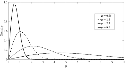
Figure 1: Rayleigh probability densities functions for $\mu\in\{0.65,1.3,2.7,5.5\}$.

The Rayleigh regression model is defined assuming that the mean $\mu[n]$ of the observed output signal $Y[n]$ can be written as

$$\eta[n]=g(\mu[n])=\sum_{i=1}^{k}\beta_{i}x_{i}[n],\quad n=1,2,\ldots,N,$$ (4)

where $k<N$ is the number of covariates considered in the model, $\bm{\beta}=(\beta_{1},\beta_{2},\ldots,\beta_{k})^{\top}$ is the vector of unknown parameters, $\mathbf{x}[n]=(x_{1}[n],x_{2}[n],\ldots,x_{k}[n])^{\top}$ is the vector of deterministic independent input variables, $g:\mathbb{R}^{+}\!\rightarrow\mathbb{R}$ is a strictly monotonic and twice differentiable link function, and $\eta[n]$ is the linear predictor. Parameter estimation based on the maximum likelihood method, diagnostic measures, and further mathematical properties, including large data record results, are fully discussed in [29].

1.2 Robust Estimation

Robust parameter estimation of the Rayleigh regression model can be performed by the weighted maximum likelihood approach [11]. Given a known weighted vector $\mathbf{w}=(w[1],w[2],\ldots,w[N])^{\top}$, the weighted maximum likelihood estimates are given by

$$\widehat{\bm{\beta}}=\arg\max_{\bm{\beta}}\ell_{w}(\bm{\beta}),$$ (5)

where $\ell_{w}(\bm{\beta})$ is the weighted log-likelihood function of the parameters for the observed signal, defined as

$$\ell_{w}(\bm{\beta})=\sum_{n=1}^{N}w[n]\ell[n](\mu[n]).$$ (6)

The quantity $\ell[n](\mu[n])$ is the logarithm of $f(y[n],\mu[n])$, which is written as

$$\begin{split}\ell[n](\mu[n])=&\log\left(\frac{\pi}{2}\right)+\log(y[n])\\ &-\log(\mu[n]^{2})-\frac{\pi y[n]^{2}}{4\mu[n]^{2}},\end{split}$$ (7)

where $\mu[n]=g^{-1}\left(\sum_{i=1}^{k}x_{i}[n]\beta_{i}\right)$. The weighted score vector, obtained by differentiating the weighted log-likelihood function with respect to each unknown parameters $\beta_{i}$, $i=1,2,\ldots,k$, is given by

$$U_{w}(\bm{\beta})=\left(\frac{\partial\ell_{w}(\bm{\beta})}{\partial\beta_{1}},\frac{\partial\ell_{w}(\bm{\beta})}{\partial\beta_{2}},\ldots,\frac{\partial\ell_{w}(\bm{\beta})}{\partial\beta_{k}}\right)^{\top}.$$ (8)

Considering the chain rule, we have that

$$\frac{\partial\ell_{w}(\bm{\beta})}{\partial\bm{\beta}}=\sum_{n=1}^{N}w[n]\frac{d\ell[n](\mu[n])}{d\mu[n]}\frac{d\mu[n]}{d\eta[n]}\frac{\partial\eta[n]}{\partial\bm{\beta}}.$$ (9)

As reported in [29], note that

$$\frac{d\ell[n](\mu[n])}{d\mu[n]} =\frac{\pi y[n]^{2}}{2\mu[n]^{3}}-\frac{2}{\mu[n]},$$ (10)

$$\frac{d\mu[n]}{d\eta[n]} =\frac{1}{g^{\prime}(\mu[n])},$$ (11)

$$\frac{\partial\eta[n]}{\partial\beta_{i}} =x_{i}[n],$$ (12)

where $g^{\prime}(\cdot)$ is the first derivative of the adopted link function $g(\cdot)$. In matrix form, the weighted score vector can be written as

$$U_{w}(\bm{\beta})=\mathbf{X}^{\top}\cdot\mathbf{W}\cdot\mathbf{T}\cdot\mathbf{v},$$ (13)

where $\mathbf{X}$ is an $N\times k$ matrix whose $n$th row is $\mathbf{x}[n]^{\top}$, and

$$\mathbf{W}= \operatorname{diag}\{w[1],w[2],\ldots,w[N]\},$$

$$\mathbf{T}= \operatorname{diag}\left\{\frac{1}{g^{\prime}(\mu[1])},\frac{1}{g^{\prime}(\mu[2])},\ldots,\frac{1}{g^{\prime}(\mu[N])}\right\},$$

$$\mathbf{v}\!= \!\left(\!\frac{\pi y[1]^{2}}{2\mu[1]^{3}}\!-\!\frac{2}{\mu[1]},\frac{\pi y[2]^{2}}{2\mu[2]^{3}}\!-\!\frac{2}{\mu[2]},\ldots,\frac{\pi y[N]^{2}}{2\mu[N]^{3}}\!-\!\frac{2}{\mu[N]}\!\right)\!^{\top}\!\!.$$

Thus, the weighted maximum likelihood estimator (WMLE) for each Rayleigh regression model parameter is obtained by solving the following nonlinear system

$$U_{w}(\bm{\beta})=\mathbf{0},$$ (14)

where $\mathbf{0}$ is the $k$-dimensional vector of zeros. The quasi-Newton Broyden-Fletcher-Goldfarb-Shanno (BFGS) method [30] with analytic first derivatives was considered as the nonlinear optimization algorithm to solve (14). To determine the initial points, we followed the same methodology described in [29].

1.2.1 Weighted Vector Determination

The WMLE is obtained supposing that the weights $w[n]$, $n=1,2,\ldots,N$, are known. However, in practice, we have to determine these values. As suggested by [11], we consider the following approach for the weighted vector determination:

$$w[n]=\begin{cases}\frac{F(y[n];\mu[n])}{\delta},&\text{if}\,\,F(y[n];\mu[n])<\delta,\\ 1,&\text{if}\,\,\delta\leq F(y[n];\mu[n])\leq 1-\delta,\\ \frac{1-F(y[n];\mu[n])}{\delta},&\text{if}\,\,F(y[n];\mu[n])>1-\delta,\end{cases}$$ (15)

where $\delta\in(0,1)$ is employed to delimit the weighed distribution interval in $(1-2\delta)\%$ and the unknown parameter is replaced by their non-robust maximum likelihood estimator (MLE). Typical values for $\delta$ are $0.01$ and $0.001$ [11]. We note that atypical $y[n]$ values imply in large or small $F(y[n];\mu[n])$ values, which are weighted; consequently, inference distortions related to these observations are minimized.

1.3 Testing Inference

Under the following mild regularity conditions: (i) the first- and second-order derivatives of the weighted log-likelihood function are well-defined; and (ii) the expectation of the score function is equal to zero, it is shown in [11] and [18] that the WMLEs are asymptotically equivalent to the MLEs. Thus, we can use the classical Wald statistic to make inferences about the regression parameters. Suppose that we partition the parameter vector $\bm{\beta}$ into a vector of parameters of interest ($\bm{\beta}_{I}$), with dimension $\nu$, and in a nuisance parameter vector ($\bm{\beta}_{M}$), with dimension $k-\nu$. The interest hypothesis $\mathcal{H}_{0}$ and the alternative hypothesis $\mathcal{H}_{1}$ are given by

$$\begin{cases}\mathcal{H}_{0}:\bm{\beta}_{I}=\bm{\beta}_{I0},\\ \mathcal{H}_{1}:\bm{\beta}_{I}\neq\bm{\beta}_{I0},\end{cases}$$ (16)

where $\bm{\beta}_{I0}$ is a fixed column vector of dimension $\nu$. The Wald statistic is given by [20]

$$T_{W}=(\widehat{\bm{\beta}}_{I1}-\bm{\beta}_{I0})^{\top}\left(\left[\mathbf{I}^{-1}(\widehat{\bm{\beta}}_{1})\right]_{\beta_{I}\beta_{I}}\right)^{-1}(\widehat{\bm{\beta}}_{I1}-\bm{\beta}_{I0}),$$ (17)

where $\widehat{\bm{\beta}}_{1}=(\widehat{\bm{\beta}}_{I1}^{\top},\widehat{\bm{\beta}}_{M1}^{\top})^{\top}$ is the WMLE under $\mathcal{H}_{1}$, $\mathbf{I}(\widehat{\bm{\beta}})$ is the Fisher information matrix derived in [29] evaluated at the WMLE, and $\left[\mathbf{I}^{-1}(\widehat{\bm{\beta}})\right]_{\beta_{I}\beta_{I}}$ is a partition of $\mathbf{I}(\widehat{\bm{\beta}})$ limited to the interest estimates. The Fisher information matrix is given by $\mathbf{I}(\bm{\beta})=\mathbf{X}^{\top}\cdot\mathbf{W}\cdot\mathbf{X}$, where

$$\begin{split}\mathbf{W}&=\operatorname{diag}\left\{\frac{4}{\mu[1]^{2}}\left(\dfrac{d\mu[1]}{d\eta[1]}\right)^{2},\frac{4}{\mu[2]^{2}}\left(\dfrac{d\mu[2]}{d\eta[2]}\right)^{2},\ldots,\right.\\ &\left.\frac{4}{\mu[N]^{2}}\left(\dfrac{d\mu[N]}{d\eta[N]}\right)^{2}\right\}.\end{split}$$ (18)

In particular, for the log link function ($g(\mu[n])=\log(\mu[n])$), the Fisher information matrix is exactly the same for the robust and non-robust approaches, since $\dfrac{d\mu[n]}{d\eta[n]}=\mu[n]$.

Based on the consistency of the WMLE and the asymptotic normality of the estimators, $T_{W}$ statistic follows, in large data records, a chi-square distribution with $\nu$ degrees of freedom, $\chi^{2}_{\nu}$. The test is performed by comparing the calculated value of $T_{W}$ with a threshold value, $\gamma$, obtained from the $\chi^{2}_{\nu}$ distribution and the desired probability of false alarm [20]. The Wald test described above can be used for several detection signal applications, such as ground type use and presence of a signal.

2 Simulation Study

This section considers Monte Carlo simulations to evaluate the finite signal length performance of the robust point estimators of the Rayleigh regression model parameters. For such, we assess the estimation performance with and without outliers. We also measure the estimator sensitivity in the presence of anomalous observations and the breakdown point.

2.1 Robust Point Estimators Performance

The numerical evaluation was made over $5,000$ different signal samples generated by means of (4) and considering the log link function. Following the methodology described in [29], the parameters were adopted as follows: $\beta_{1}=0.5$ and $\beta_{2}=0.15$, and the covariate was obtained from the uniform distribution $(0,1)$, and considered constants for all Monte Carlo replications. In each replication, the inversion method was employed to simulate $y[n]$ assuming the Rayleigh distribution with mean $\mu[n]=\exp\left\{\beta_{1}+\beta_{2}x_{2}[n]\right\}$.

The simulation study considered signals in several situations, varying the sample size $N\in\{100,\,500,\,750\}$ and the contamination level $\epsilon\in\{0\%,1\%,5\%\}$. The selected values of $\epsilon$ follow the literature as shown in [2], [7], and [4] for robust estimation analysis in one-, two-, and three-dimensional models, respectively. The outliers were included, assuming a value equal to $10$ in randomized positions. We employed $\delta\in\{0.001,0.01\}$ for the weight determination; however, for brevity and similarity of results, just the ones for $\delta=0.001$ are shown. The percentage relative bias (RB%), the mean square error (MSE), and the sum of the absolute values of RB% and MSE total were adopted as figures of merit to numerically evaluate the proposed robust estimators. Such error measures are expected to be as small as possible and were computed between $\bm{\beta}$ and $\bm{\widehat{\beta}}$.

Table 1 shows the Monte Carlo simulation results for the point estimators of the Rayleigh regression model parameters with and without outliers. Both WMLEs and MLEs show similar and small values of RB% and MSE for the data without outliers. In particular, the absolute total value of relative bias for $N=100$ is equal to $1.6228$ and $1.5765$ for WMLE and MLE, respectively. However, the MLEs present higher values of RB% and MSE for the contaminated data when compared to the WMLE results, showing that the robust theory is effective, reducing considerably the RB% and MSE values concerning the non-robust estimation method in corrupted signals. For instance, consider the case with $5\%$ of contamination and $N=500$, the WMLE for $\beta_{1}$ displays values of RB% equal to $1.8567\%$, while the MLE shows RB% value about $106\%$ for the same parameter. Summarizing, the WMLEs show either equal or better performance compared with the results from the MLEs, in all evaluated cases.

Table 1: Results of the Monte Carlo simulation of the point estimation considering the robust (WMLE) and non-robust (MLE) approaches, with and without outliers, for $\beta_{1}=0.5$, $\beta_{2}=0.15$, and $\delta=0.001$

		WMLE			MLE
$\epsilon$	Measures	$\widehat{\beta}_{1}$	$\widehat{\beta}_{2}$	Absolute Total	$\widehat{\beta}_{1}$	$\widehat{\beta}_{2}$	Absolute Total
$N=100$
$0\%$	Mean	$0.4957$	$0.1488$	—	$0.4967$	$0.1486$	—
	RB(%)	$-0.8570$	$-0.8259$	$1.6828$	$-0.6598$	$-0.9167$	$1.5765$
	MSE	$0.0100$	$0.0312$	$0.0413$	$0.0099$	$0.0309$	$0.0409$
$1\%$	Mean	$0.4968$	$0.1480$	—	$0.6401$	$0.1247$	—
	RB(%)	$-0.6311$	$-1.3311$	$1.9622$	$28.0262$	$-16.8944$	$44.9206$
	MSE	$0.0101$	$0.0316$	$0.0417$	$0.0715$	$0.1916$	$0.2631$
$5\%$	Mean	$0.5476$	$0.1597$	—	$1.0103$	$0.0705$	—
	RB(%)	$9.5122$	$6.4767$	$15.9889$	$102.0672$	$-53.0026$	$155.0698$
	MSE	$0.0518$	$0.1693$	$0.2211$	$0.3405$	$0.3098$	$0.6503$
$N=500$
$0\%$	Mean	$0.4974$	$0.1508$	—	$0.4989$	$0.1508$	—
	RB(%)	$-0.5234$	$0.5316$	$1.0550$	$-0.2291$	$0.5216$	$0.7507$
	MSE	$0.0021$	$0.0062$	$0.0083$	$0.0020$	$0.0061$	$0.0081$
$1\%$	Mean	$0.4989$	$0.1506$	—	$0.6579$	$0.1183$	—
	RB(%)	$-0.2117$	$0.4203$	$0.6320$	$31.5790$	$-21.1080$	$52.6870$
	MSE	$0.0021$	$0.0062$	$0.0083$	$0.0362$	$0.0425$	$0.0786$
$5\%$	Mean	$0.5093$	$0.1628$	—	$1.0314$	$0.0679$	—
	RB(%)	$1.8567$	$8.5400$	$10.3967$	$106.2793$	$-54.7086$	$160.9879$
	MSE	$0.0045$	$0.0162$	$0.0208$	$0.2954$	$0.0566$	$0.3519$
$N=750$
$0\%$	Mean	$0.4980$	$0.1507$	—	$0.4996$	$0.1506$	—
	RB(%)	$-0.3962$	$0.4568$	$0.8530$	$-0.0875$	$0.4140$	$0.5015$
	MSE	$0.0014$	$0.0041$	$0.0054$	$0.0014$	$0.0040$	$0.0054$
$1\%$	Mean	$0.4997$	$0.1507$	—	$0.6673$	$0.1184$	—
	RB(%)	$-0.0593$	$0.4608$	$0.5201$	$33.4529$	$-21.0987$	$54.5516$
	MSE	$0.0014$	$0.0041$	$0.0054$	$0.0360$	$0.0300$	$0.0660$
$5\%$	Mean	$0.5080$	$0.1631$	—	$1.0359$	$0.0698$	—
	RB(%)	$1.6012$	$8.7438$	$10.3450$	$107.1780$	$-53.4431$	$160.6211$
	MSE	$0.0027$	$0.0099$	$0.0127$	$0.2959$	$0.0396$	$0.3355$

2.2 The Breakdown Point and Sensibility Curve

The breakdown point was proposed in [17] and evaluate the proportion of outliers that the signal may contain such that $\widehat{\bm{\beta}}$ still provides some information about the true parameter [17, 44, 47]. Figure 2(a) displays the total breakdown point in terms of the total relative bias of the estimators, which is defined as the sum of the absolute values of the individual relative biases. As in the robust estimators point evaluation, the outlier value was set equal to $10$. Additionally, we employed $1000$ Monte Carlo replications and the number of outliers ranging from $1$ to $100$. We note that the WMLEs show smaller total relative bias values compared with the results from the MLEs, in all evaluated cases. In general, we note that for $1\%$ of contamination, the MLEs present total relative bias close to or higher than $100$. On the other hand, the WMLEs show the same total relative bias values for a contamination level of about $10\%$ of the observations.

(a) Total breakdown point

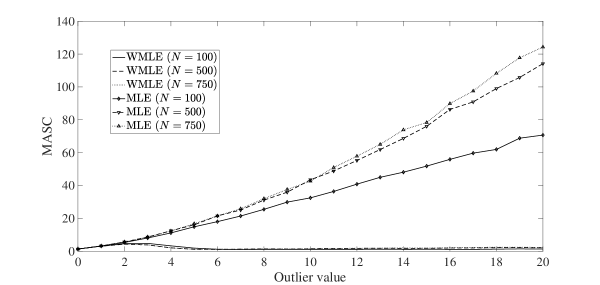
(b) Sensitivity curves

Figure 2: The total breakdown point and sensitivity results considering $5\%$ of outliers and $1000$ Monte Carlo replications.

Another measure widely used to evaluate robust estimators is the sensitivity curve (SC) [47], which provides an intuitive information about the sensitivity of an estimator measuring its variability with the addition of an outlier to the signal. The SC is given by [47]

$$\begin{split}\text{SC}(\mathbf{y},\bm{\widehat{\beta}})&=N\cdot\left(\bm{\widehat{\beta}}(y[1],y[2],\ldots y[N-1],y_{\text{out}})-\right.\\ &\left.\bm{\widehat{\beta}}(y[1],y[2],\ldots y[N-1])\right),\end{split}$$ (19)

where $\bm{\widehat{\beta}}(y[1],y[2],\ldots y[N-1])$ is the estimator without outliers and $\bm{\widehat{\beta}}(y[1],y[2],\ldots y[N-1],y_{\text{out}})$ is the estimator contaminated with an outlier $y_{\text{out}}$. For a better graphical analysis, the SC results are shown as the mean absolute value of SC (MASC) of all estimators. This unified measure was proposed in [4] for multiparametric evaluations.

The MASC considering $5\%$ of outliers with their values ranging from $1$ to $20$ and $1000$ Monte Carlo replications is presented in Figure 2(b), showing that the WMLE is more robust to outliers when compared to the MLE, for all evaluated outlier values and signal lengths. The MLE displays a MASC maximum value of about $130$, while the WMLE does not show values higher than $5$. Additionally, the WMLEs present similar behavior regardless of the evaluated signal length and outlier value, whereas the MLEs display higher MASC values as the signal length and the outlier value increases.

In summary, the Monte Carlo simulations show that the robust-based Rayleigh regression model parameter estimators are not strongly influenced by the presence or absence of outliers in the observed signal. Furthermore, in real-world scenarios, identifying whether a signal is contaminated by outliers is not an easy task. Thus, using a robust approach to estimate the parameters of the Rayleigh regression model can avoid inaccurate inferences.

3 SAR Image Study

In this section, experiments with two measured SAR data sets are presented to demonstrate the applicability of the proposed approach in SAR image analysis. We employed the introduced robust scheme to detect ground type and anomalies in SAR image scenes. In particular, VHF wavelength-resolution SAR images are almost speckle-free, since there might only be a single scatter in the resolution cell (at least for the CARABAS II data set). On the other hand, non-wavelength-resolution SAR images are characterized by the possible presence of more than one strong scatter in the resolution cell area, which makes the speckle noise not negligible. We emphasize that the speckle and other random effects are accommodated in the Rayleigh-distributed output signal $Y[n]$. The regression structure models the mean of $Y[n]$ which is deterministically affected by parameters and known covariates (input).

3.1 Ground Type Detector

In this experiment, we considered the ground type detection methodology used in [29] to distinguish between three regions in two SAR images extracted from CARABAS II and OrbiSAR data sets considering the proposed robust approach.

3.1.1 CARABAS II

As reported in [21] and [39], the CARABAS II is a VHF wavelength-resolution system, which means that the images have almost no speckle noise. The system operates with horizontal (HH) polarization, and the spatial resolution is $2.5\leavevmode\nobreak\ \text{m}$ in both azimuth and slant range. The CARABAS II images are (i) represented as matrices of $3000\times 2000$ pixels (each pixel size is $1\,\text{m}\times 1\,\text{m}$), corresponding to an area of $6\leavevmode\nobreak\ \text{km}^{2}$, covering a scene of size $3\,\text{km}\times 2\,\text{km}$; (ii) georeferenced to the Swedish reference system RR92; and (iii) available in [33].

The ground scene is dominated by boreal forest with pine trees. Fences, power lines, and roads were also present in the scene. Military vehicles (targets) were deployed in the SAR scene and placed uniformly in a manner to facilitate their detection in the tests [21]. The image has $25$ targets of three different sizes, and the spacing between the vehicles is about 50 meters.

In [29], it was computed the difference in the behavior among the lake, forest, and military vehicles region. The forest and lake regions in the CARABAS II SAR image characterize most of the image area, and they follow a homogeneous pattern. The military vehicles deployed in the SAR scene introduce more representative behavior changing when compared to the forest and lake regions (homogeneous areas). Additionally, pixels related to the power lines show similar amplitude values with the targets and, consequently, are strongly related to the false alarm detection in this particular data set, as discussed in [21]. Furthermore, as both targets and power line structures present a different pattern from the rest of the image, they may be considered as anomalies observations (outliers).

Thus, we adopted the detection methodology proposed in [29] to distinguish among an area containing military vehicles, power lines, and forests—referred to as Regions A, B, and C, respectively—, which are displayed in Figure 3. For such, we modeled the response signal mean considering an intercept, $x_{1}[n]=1,\,\forall n$, and two dummy variables, $x_{2}[n]$ and $x_{3}[n]$, representing each evaluated region. The fitted model is given by

$$g(\mu[n])=\beta_{1}+\beta_{2}x_{2}[n]+\beta_{3}x_{3}[n],$$ (20)

where (i) $y[n]$ is the vectorized magnitude pixels of Regions A, B, and C; (ii) variable $x_{2}[n]=1$, for Region B, and zero for the rest; (iii) variable $x_{3}[n]=1$, for Region C, and zero for the others; and (iv) Region A is represented for both $x_{2}[n]$ and $x_{3}[n]$ equal to zero.

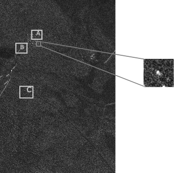
Figure 3: CARABAS II image used in the regression models showing the tested regions. Regions A, B, and C represent areas containing military vehicles, power lines, and forest, respectively.

To detect the ground type, the following hypotheses are tested

$$\begin{cases}\mathcal{H}_{0}:\beta_{i}=0,\\ \mathcal{H}_{1}:\beta_{i}\neq 0,\end{cases}$$ (21)

for $i=2,3,\ldots,k$. The evaluated ground types are detected when the null hypothesis (21) is rejected, i.e., $T_{W}>\gamma$. We also obtained the detection results based on (i) the Gaussian and Gamma regression models considering a robust estimation process and (ii) the Rayleigh regression model based on the maximum likelihood estimation scheme for comparative purposes. To implement the detectors through the Gaussian- and Gamma-based regression models considering a robust approach, the R function glmrob [31] was used. To perform the ground type detection, the probability of false alarm was fixed to $0.05$, which is a convenient cutoff level to reject the null hypothesis [12], and it is widely employed in signal detection applications [34, 32, 22, 43].

The fitted models can be found in Table 2. Note that the estimated values are not the same as those presented in [29], since we evaluated different regions in the present experiment. To perform the robust estimation in the Rayleigh regression model, we employed $\delta=0.001$. Considering a probability of false alarm equal to $0.05$, the $p$-values of the Wald test presented in Table 2 show that all variables in the proposed robust scheme are significant, i.e., the null hypothesis in (21) can be rejected, and consequently, a correct detection of all evaluated land types is indicated. On the other hand, the variable $x_{2}[n]$ is not significant for the other evaluated regression models, i.e., Rayleigh regression model based on non-robust estimation process and the models using the Gaussian- and Gamma-based on a robust estimation process can not distinguish the power line regions, showing the importance of robust methods based on suitable distributions to deal with outliers in SAR image modeling.

Table 2: Fitted regression models for Regions A, B, and C

	Estimate	Standard Error	$p$-value
Rayleigh regression model (robust estimators)
$\widehat{\beta}_{1}$	$-1.6681$	$0.0333$	$<0.001$
$\widehat{\beta}_{2}$	$0.1168$	$0.0521$	$0.0250$
$\widehat{\beta}_{3}$	$-0.4993$	$0.0521$	$<0.001$
Rayleigh regression model (non-robust estimators)
$\widehat{\beta}_{1}$	$-1.4916$	$0.0333$	$<0.001$
$\widehat{\beta}_{2}$	$-0.0555$	$0.0521$	$0.2867$
$\widehat{\beta}_{3}$	$-0.6759$	$0.0521$	$<0.001$
Gaussian regression model (robust estimators)
$\widehat{\beta}_{1}$	$0.1896$	$0.0090$	$<0.001$
$\widehat{\beta}_{2}$	$0.0098$	$0.0140$	$0.4870$
$\widehat{\beta}_{3}$	$-0.0738$	$0.0140$	$<0.001$
Gamma regression model (robust estimators)
$\widehat{\beta}_{1}$	$5.5817$	$0.2558$	$<0.001$
$\widehat{\beta}_{2}$	$-0.4396$	$0.3823$	$0.2500$
$\widehat{\beta}_{3}$	$2.6408$	$0.5209$	$<0.001$

3.1.2 OrbiSAR

The SAR image was acquired with the airborne OrbiSAR sensor of Bradar over São José dos Campos, Brazil. As reported in [3] and [35], the OrbiSAR is an airborne multipolarized dual-band SAR system of Bradar (formerly Orbisat), Brazil, that operates at X-band with HH polarization and spatial resolution of $1\,\text{m}$, and at P-band with full polarization—HH, vertical (VV), VH, and HV—and spatial resolution of $2\,\text{m}$, with three antennas mounted on the same platform allowing repeat-pass and multibaseline interferometry, at P- and X-bands, respectively. The system is also equipped with a state-of-the-art navigation system and motion compensation [35]. Additionally, the bandwidth and the radar swath can be up to 400 MHz and 14 km, respectively [35].

Figure 4 shows an X-band SAR image acquired with the OrbiSAR system. The image is represented in a $2500\times 3150$ matrix of magnitude data. The ground scene of the considered image is dominated by urban area (light ground–top and bottom right area), rivers (dark ground–bottom and left part of the image), forests, roads, and open areas (gray ground). The urban area presents a different pattern from the rest of the image and may be considered outliers.

To perform the ground type detection in the X-band SAR image, we adopted the same methodology described in the previous subsection to distinguish among an open area, a road, and an urban land type—referred to as Regions D, E, and F, respectively. Figure 4 shows the three different evaluated regions. The mean of the response signal was modeled using the model presented in (20), where the response signal is composed of the vectorized magnitude pixels of the Regions D, E, and F, and $x_{2}[n]$ and $x_{3}[n]$ are dummy variables related to regions E and F, respectively.

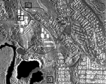
Figure 4: OrbiSAR image used in the regression models showing the tested regions. Regions D, E, and F represent an open area, a road, and an urban land type, respectively.

The fitted models are shown in Table 3, with $\delta=0.001$ for the proposed method. The $p$-values show that all variables in Rayleigh and Gamma regression models considering a robust estimation process are significant for a probability of false alarm equal to $0.05$, i.e., the null hypothesis in (21) can be rejected, indicating a correct detection of all evaluated ground types. In contrast, the variable $x_{2}[n]$ is not significant for the non-robust Rayleigh regression method and robust Gaussian approach, i.e., these models can not distinguish the road region, evidencing the importance of suitable models to deal with outliers in SAR image modeling.

Table 3: Fitted regression models for Regions D, E, and F

	Estimate	Standard Error	$p$-value
Rayleigh regression model (robust estimators)
$\widehat{\beta}_{1}$	$-0.6069$	$0.0423$	$<0.001$
$\widehat{\beta}_{2}$	$-0.1190$	$0.0598$	$0.0464$
$\widehat{\beta}_{3}$	$2.7767$	$0.1319$	$<0.001$
Rayleigh regression model (non-robust estimators)
$\widehat{\beta}_{1}$	$-0.6069$	$0.0423$	$<0.001$
$\widehat{\beta}_{2}$	$-0.1105$	$0.0598$	$0.0646$
$\widehat{\beta}_{3}$	$2.6749$	$0.1319$	$<0.001$
Gaussian regression model (robust estimators)
$\widehat{\beta}_{1}$	$0.6087$	$0.1038$	$<0.001$
$\widehat{\beta}_{2}$	$-0.0777$	$0.1468$	$0.5970$
$\widehat{\beta}_{3}$	$6.6209$	$0.3241$	$<0.001$
Gamma regression model (robust estimators)
$\widehat{\beta}_{1}$	$1.6312$	$0.0338$	$<0.001$
$\widehat{\beta}_{2}$	$0.2542$	$0.0517$	$<0.001$
$\widehat{\beta}_{3}$	$-1.5122$	$0.0346$	$<0.001$

3.2 Anomaly Detection

We propose a detection scheme to detect anomalies in a SAR image considering the Rayleigh regression model residuals. Our methodology aims at detecting area changes, measuring the deviations of the observed pixel values $y[n]$ from their estimated mean values $\widehat{\mu}[n]$. For such, we use the quantile residuals [10], which are defined as

$$r[n]=\Phi^{-1}\left(F(y[n];\widehat{\mu}[n])\right),$$ (22)

where $\Phi^{-1}$ denotes the standard normal quantile function. The quantile residual can detect poor fitting in regression models and follows an approximately standard Gaussian distribution [10] if the model is correctly specified. If the estimated mean of the response signal is too far from the observed pixel value—which can be highlighted by the residual values—then an anomaly is detected. To capture a model mismatch, we adopt residual based control charts, which have been already used in change detection in remote sensing data, e.g., in [4] and [6]. The introduced anomaly detection methodology is based on the following premises:

• If the model is correctly fitted, then it is expected that the residuals are randomly distributed around zero and inside the interval $[-3,\,3]$, about $99.7\%$ of the observations $\left(2\Phi(L)-1|_{L=3}\approx 99.7\%\right)$. Consequently, the control limit $L$ can be set equal to three [6, 5].

• If the residual value is outside the interval $[-3,\,3]$, then the analyzed pixel is understood to differ from the expected behavior according to the Rayleigh regression model fitted in the region of interest and, consequently, an anomaly is detected.

A post-processing step using mathematical morphological operations, such as erosion, dilation, opening, and closing operations, can be considered aiming at (i) removing small spurious pixel groups which are regarded as noise and (ii) preventing the splitting of the interest objects into multiple substructures [15]. The anomaly detection method used in the current experiment is summarized in Algorithm 1.

Algorithm 1 Anomaly detection method based on the robust Rayleigh regression method

0:  Interest image $\mathbf{X}_{\text{I}}$

0:  Detected results $\mathbf{X}_{\text{D}}$

  1) Select a region of interest (training sample) $\mathbf{X}_{\text{S}}\subset\mathbf{X}_{\text{I}}$.

  2) Fit the robust Rayleigh regression method considering the $\mathbf{X}_{\text{S}}$ image.

  3) Using the fitted model obtained in 2), compute the residuals $r[n]$ of $\mathbf{X}_{\text{I}}$.

  4) Obtain a binary images as follows:

  if $(r[n]\leq L)\,\,\,\text{or}\,\,\,(r[n]\geq L)$ then

     $X^{\star}[n]\leftarrow 1$

  else

     ${X}^{\star}[n]\leftarrow 0$.

  end if

  5) Apply morphological operators as a final post-processing step: $\mathbf{X}_{\text{D}}\leftarrow\text{post-processing}(\mathbf{X}^{\star})$.

To perform the proposed detection method in a CARABAS II SAR image, we selected a region containing military vehicles (anomalies), as shown in the dark gray rectangle in Figure 3. This region has about $5\%$ of the observations related to outliers. According to the Monte Carlo simulations, the WMLEs in the Rayleigh regression model are not strongly influenced by the presence or absence of outliers in the observed signal. Additionally, because in practical situations it is difficult to identify whether there are outliers or not in the training sample, we selected as $\mathbf{X}_{\text{S}}$ a region with anomaly observations to highlight the importance of using a robust approach to deal with outliers.

To fit the regression model, we considered as covariates the other three images with the same flight pass available in the CARABAS II data set to describe the amplitude mean value of the CARABAS II image pixels. The model is specified for the response signal mean as follows

$$g(\mu[n])=\beta_{1}+\beta_{2}x_{2}[n]+\beta_{3}x_{3}[n]+\beta_{4}x_{4}[n].$$ (23)

The response signal is composed of the vectorized amplitude values of the training sample pixels. Variables $x_{2}[n]$, $x_{3}[n]$, and $x_{4}[n]$ are the vectorized magnitude pixels of the images related to pass one and missions two, three, and four, respectively. As we expect to have outliers in the observed signal and not in the covariates, $x_{2}[n]$, $x_{3}[n]$, and $x_{4}[n]$ represent a forest area. For the post-processing step, we employed an opening operation—considering a $3\times 3\leavevmode\nobreak\ \text{pixels}$ square structuring element, whose size is linked by the system resolution—followed by a dilation—using $7\times 7\leavevmode\nobreak\ \text{pixels}$ structuring element which is related to the approximate size of the military vehicles. Using such operations, we kept the criterion defined in [21], i.e., detection with less than ten meters apart are merged as one.

The anomaly detection results can be found in Figure 5. We compared the detection results of the Rayleigh regression models considering a robust and non-robust estimation process, which are displayed in Figure 5. The robust method detected $24$ military vehicles and two false alarms. In contrast, the non-robust scheme can only detect $23$ military vehicles and shows $15$ false alarms. In particular, the false alarms in the non-robust method are related to the power lines area; this result is in accordance with the ones presented in the Section 3.1, showing that, in both experiments, the non-robust estimation process can not distinguish between the targets and power line areas, and consequently, evidencing the importance of a robust approach to deal with outliers.

(a) Detections: Robust-based estimation

(b) Detections: Non-robust-based estimation

Figure 5: Detection results based on the robust and non-robust estimation of the Rayleigh regression model parameters.

We also compared the proposed methodology with three different approaches presented in [28], [21], and [41]; the performance of the proposed scheme was very close to the competing methods specifically developed to this aim: only one less detection hit; and two more false alarms than the results showed in [28] and [41]. On the one hand, the accurate performance of such methods is related to a optimized threshold choice. On the other hand, our proposed anomaly detection method shows accurate detection results avoiding this step, since the residual-based control chart has a fixed theoretical threshold ($L=3$). The detection results of all evaluated methods are summarized in Table 4.

Table 4: Number of Detected Targets and False Alarms obtained considering the Rayleigh regression models based on robust and non-robust approaches, and the methods in [28], [21], and [41]

Method	Detected Targets	False Alarm
Robust Approach	$24$	$2$
Non-robust Approach	$24$	$15$
Method in [28]	$25$	$0$
Method in [21]	$25$	$2$
Method in [41]	$25$	$0$

4 Conclusions

This paper introduced robust estimators for the Rayleigh regression model parameters. In particular, we employed the weighted maximum likelihood approach to obtain estimators that are robust to the presence of outliers. Monte Carlo simulation results showed that the WMLEs outperformed traditional MLEs in terms of relative bias and root mean square error. In particular, the non-robust estimators presented a relative bias value $65$-fold larger than the results provided by the robust estimators in signals corrupted with outliers. In terms of sensitivity analysis and break down point, the robust approach resulted in a reduction of about $96\%$ and $10\%$ in the mean absolute value in compassion to the non-robust estimators. For non-contaminated signals, both schemes had similar behavior. Two studies considering the proposed robust approach in the Rayleigh regression model parameter estimation to distinguish between different regions in a SAR image were presented and discussed, showing competitive detection results compared to the non-robust Rayleigh-, robust Gaussian-, and robust Gamma-based measurements. Moreover, we proposed an anomaly detector based on the Rayleigh regression model. The robust estimation approach excelled in terms of detection when compared to the non-robust estimators of the Rayleigh regression model parameters, and it offered very close results to those reported in [28], [21], and [41], i.e., only one less detection hit; and two more false alarms than the results showed in [28] and [41].

References

- [1] H. Allende, J. Galbiati, and R. Vallejos, Robust image modeling on image processing, Pattern Recognition Letters, 22 (2001), pp. 1219–1231.
- [2] H. Allende and L. Pizarro, Robust estimation of roughness parameter in SAR amplitude images, in Iberoamerican Congress on Pattern Recognition, Springer, 2003, pp. 129–136.
- [3] T. L. Barreto, R. A. Rosa, C. Wimmer, J. R. Moreira, L. S. Bins, F. A. M. Cappabianco, and J. Almeida, Classification of detected changes from multitemporal high-res Xband SAR images: Intensity and texture descriptors from SuperPixels, IEEE Journal of Selected Topics in Applied Earth Observations and Remote Sensing, 9 (2016), pp. 5436–5448.
- [4] D. M. Bayer, F. M. Bayer, and P. Gamba, A 3-D spatiotemporal model for remote sensing data cubes, IEEE Transactions on Geoscience and Remote Sensing, 59 (2021), pp. 1082–1093.
- [5] F. M. Bayer, A. J. Kozakevicius, and R. J. Cintra, An iterative wavelet threshold for signal denoising, Signal Processing, 162 (2019), pp. 10–20.
- [6] E. B. Brooks, R. H. Wynne, V. A. Thomas, C. E. Blinn, and J. W. Coulston, On-the-fly massively multitemporal change detection using statistical quality control charts and Landsat data, IEEE Transactions on Geoscience and Remote Sensing, 52 (2013), pp. 3316–3332.
- [7] O. Bustos, S. Ojeda, and R. Vallejos, Spatial ARMA models and its applications to image filtering, Brazilian Journal of Probability and Statistics, 23 (2009), pp. 141–165.
- [8] O. H. Bustos, M. Lucini, and A. C. Frery, M-estimators of roughness and scale for-modelled SAR imagery, EURASIP Journal on Advances in Signal Processing, 2002 (2002), p. 297349.
- [9] L. Devroye, Sample-based non-uniform random variate generation, in Proceedings of the 18th conference on Winter simulation, 1986, pp. 260–265.
- [10] P. K. Dunn and G. K. Smyth, Randomized quantile residuals, Journal of Computational and Graphical Statistics, 5 (1996), pp. 236–244.
- [11] C. Field and B. Smith, Robust estimation: A weighted maximum likelihood approach, International Statistical Review/Revue Internationale de Statistique, 62 (1994), pp. 405–424.
- [12] R. A. Fisher, Statistical methods for research workers, in Breakthroughs in Statistics, Springer, 1992, pp. 66–70.
- [13] A. Ghosh and A. Basu, Robust estimation in generalized linear models: the density power divergence approach, Test, 25 (2016), pp. 269–290.
- [14] A. Ghosh, A. Basu, et al., Robust estimation for independent non-homogeneous observations using density power divergence with applications to linear regression, Electronic Journal of Statistics, 7 (2013), pp. 2420–2456.
- [15] R. C. Gonzalez and R. Woods, Digital image processing, Prentice Hall, 2008.
- [16] F. E. Grubbs, Procedures for detecting outlying observations in samples, Technometrics, 11 (1969), pp. 1–21.
- [17] F. R. Hampel, A general qualitative definition of robustness, The Annals of Mathematical Statistics, 42 (1971), pp. 1887–1896.
- [18] F. Hu and J. V. Zidek, The weighted likelihood, Canadian Journal of Statistics, 30 (2002), pp. 347–371.
- [19] J. Inglada and G. Mercier, A new statistical similarity measure for change detection in multitemporal SAR images and its extension to multiscale change analysis, IEEE Transactions on Geoscience and Remote Sensing, 45 (2007), pp. 1432–1445.
- [20] S. M. Kay, Fundamentals of statistical signal processing: Detection theory, vol. II, Prentice Hall, 1998.
- [21] M. Lundberg, L. M. Ulander, W. E. Pierson, and A. Gustavsson, A challenge problem for detection of targets in foliage, in Algorithms for Synthetic Aperture Radar Imagery XIII, vol. 6237, International Society for Optics and Photonics, 2006, p. 62370K.
- [22] S. Maleki, S. P. Chepuri, and G. Leus, Energy and throughput efficient strategies for cooperative spectrum sensing in cognitive radios, in 2011 IEEE 12th International Workshop on Signal Processing Advances in Wireless Communications, IEEE, 2011, pp. 71–75.
- [23] P. McCullagh and J. Nelder, Generalized linear models, Chapman and Hall, 2nd ed., 1989.
- [24] G. Melamed, S. R. Rotman, D. G. Blumberg, and A. J. Weiss, Anomaly detection in polarimetric radar images, International Journal of Remote Sensing, 33 (2012), pp. 1164–1189.
- [25] G. Mercier, G. Moser, and S. B. Serpico, Conditional copulas for change detection in heterogeneous remote sensing images, IEEE Transactions on Geoscience and Remote Sensing, 46 (2008), pp. 1428–1441.
- [26] J. Naranjo-Torres, J. Gambini, and A. C. Frery, The geodesic distance between models and its application to region discrimination, IEEE Journal of Selected Topics in Applied Earth Observations and Remote Sensing, 10 (2017), pp. 987–997.
- [27] C. Oliver and S. Quegan, Understanding synthetic aperture radar images, SciTech Publishing, 2004.
- [28] B. G. Palm, D. I. Alves, M. I. Pettersson, V. T Vu, R. Machado, R. J. Cintra, F. M. Bayer, P. Dammert, and H. Hellsten, Wavelength-resolution SAR ground scene prediction based on image stack, Sensors, 20 (2020), p. 2008.
- [29] B. G. Palm, F. M. Bayer, R. J. Cintra, M. I. Pettersson, and R. Machado, Rayleigh regression model for ground type detection in SAR imagery, IEEE Geoscience and Remote Sensing Letters, 16 (2019), pp. 1660–1664.
- [30] W. Press, S. Teukolsky, W. Vetterling, and B. Flannery, Numerical recipes in C: The art of scientific computing, Cambridge University Press, 2 ed., 1992.
- [31] P. Rousseeuw, C. Croux, V. Todorov, A. Ruckstuhl, M. Salibian-Barrera, T. Verbeke, M. Koller, and M. Maechler, Robustbase: Basic robust statistics, R package version 0.4-5, URL http://CRAN. R-project. org/package= robustbase, (2020).
- [32] X. Ru, Z. Liu, Z. Huang, and W. Jiang, Normalized residual-based constant false-alarm rate outlier detection, Pattern Recognition Letters, 69 (2016), pp. 1–7.
- [33] SDMS, Sensor Data Management System public web site, 2018. https://www.sdms.afrl.af.mil/index.php.
- [34] L. Sevgi, Hypothesis testing and decision making: Constant-false-alarm-rate detection, IEEE Antennas and Propagation Magazine, 51 (2009), pp. 218–224.
- [35] G. H. X. Shiroma, K. A. C. de Macedo, C. Wimmer, J. R. Moreira, and D. Fernandes, The dual-band polInSAR method for forest parametrization, IEEE Journal of Selected Topics in Applied Earth Observations and Remote Sensing, 9 (2016), pp. 3189–3201.
- [36] H. Sportouche, J.-M. Nicolas, and F. Tupin, Mimic capacity of fisher and generalized gamma distributions for high-resolution SAR image statistical modeling, IEEE Journal of Selected Topics in Applied Earth Observations and Remote Sensing, 10 (2017), pp. 5695–5711.
- [37] J. Susaki, K. Hara, K. Kajiwara, and Y. Honda, Robust estimation of BRDF model parameters, Remote Sensing of Environment, 89 (2004), pp. 63–71.
- [38] C. Tison, J.-M. Nicolas, F. Tupin, and H. Maître, A new statistical model for Markovian classification of urban areas in high-resolution SAR images, IEEE Transactions on Geoscience and Remote Sensing, 42 (2004), pp. 2046–2057.
- [39] L. M. Ulander, M. Lundberg, W. Pierson, and A. Gustavsson, Change detection for low-frequency SAR ground surveillance, IEEE Proceedings-Radar, Sonar and Navigation, 152 (2005), pp. 413–420.
- [40] V. T. Vu, Wavelength-resolution SAR incoherent change detection based on image stack, IEEE Geoscience and Remote Sensing Letters, 14 (2017), pp. 1012–1016.
- [41] V. T. Vu, N. R. Gomes, M. I. Pettersson, P. Dammert, and H. Hellsten, Bivariate gamma distribution for wavelength-resolution SAR change detection, IEEE Transactions on Geoscience and Remote Sensing, 57 (2018), pp. 1–9.
- [42] H. Wang and K. Ouchi, Accuracy of the -distribution regression model for forest biomass estimation by high-resolution polarimetric SAR: Comparison of model estimation and field data, IEEE Transactions on Geoscience and Remote Sensing, 46 (2008), pp. 1058–1064.
- [43] P. Weber, D. Theilliol, C. Aubrun, and A. Evsukoff, Increasing effectiveness of model-based fault diagnosis: A dynamic Bayesian network design for decision making, IFAC Proceedings Volumes, 39 (2006), pp. 90–95.
- [44] V. J. Yohai, High breakdown-point and high efficiency robust estimates for regression, The Annals of Statistics, 15 (1987), pp. 642–656.
- [45] Y. Zhao, B. Huang, and H. Song, A robust adaptive spatial and temporal image fusion model for complex land surface changes, Remote Sensing of Environment, 208 (2018), pp. 42–62.
- [46] A. M. Zoubir, Introduction to statistical signal processing, in Academic Press Library in Signal Processing, vol. 3, Elsevier, 2014, pp. 3–7.
- [47] A. M. Zoubir, V. Koivunen, E. Ollila, and M. Muma, Robust statistics for signal processing, Cambridge University Press, United Kingdom, 2018.