Signal Detection and Inference Based on the Beta Binomial Autoregressive Moving Average Model

This paper proposes the beta binomial autoregressive moving average model (BBARMA) for modeling quantized amplitude data and bounded count data. The BBARMA model estimates the conditional mean of a beta binomial distributed variable observed over the time by a dynamic structure including: (i) autoregressive and moving average terms; (ii) a set of regressors; and (iii) a link function. Besides introducing the new model, we develop parameter estimation, detection tools, an out-of-signal forecasting scheme, and diagnostic measures. In particular, we provide closed-form expressions for the conditional score vector and the conditional information matrix. The proposed model was submitted to extensive Monte Carlo simulations in order to evaluate the performance of the conditional maximum likelihood estimators and of the proposed detector. The derived detector outperforms the usual ARMA- and Gaussian-based detectors for sinusoidal signal detection. We also presented an experiment for modeling and forecasting the monthly number of rainy days in Recife, Brazil.

Keywords
ARMA filter, beta binomial distribution, detection, digital signal, time series.

1 Introduction

Signal detection is a fundamental task in the field of signal processing, being pivotal for decision making and information extraction [30]. Over the years, several detection methods have been developed assuming additive Gaussian noise [30, 55, 57], with decision criteria based on continuous-time waveforms [30]. In contrast, real-world data often present non-Gaussian signals [3, 35] and the Gaussianity assumption may not be enough to model several practical contexts, as illustrated, for example, in [57, 55, 28]. Furthermore, signal processing systems operate under quantized discrete-time sampled data. Quantized discrete-time signals—here referred to as digital signals—constitute a clear example of non-Gaussian data and their estimation and detection have been attracting attention over the past years [57, 56].

Quantized signals represent data according to a finite number of discrete values observed over time (e.g., 256 amplitude levels in 8-bit quantization) [46, 41]. Thus, the application of Gaussian-based detectors and hypothesis tests to non-Gaussian processes may lead to suboptimal or erroneous detectors [49]. Although unsatisfactory [17, 21], a better approach is to consider a data transformation that maps the measured signal from its original distribution into the Gaussian distribution [17, 21]. This method might offer limited results because the transformed data should be interpreted in terms of the transformed signal mean, not in terms of the measured data mean [17].

In this context, the beta binomial distribution offers another way to model quantized discrete-time signals. The beta binomial distribution has been used over the years to model bounded discrete values [34, 58], arising as a natural candidate for digital signals modeling. Nevertheless, to the best of our knowledge, a time series model based on the beta binomial distribution capable of addressing the detection problem for digital signal is absent in the literature.

Besides quantized signal processing applications, the derived model can be used to fit any bounded count data observed over the time, such as the number of rainy days per time interval [23], number of defective products in one lot [39], or number of hospital admissions [4]. In particular, the monitoring of the number of rainy days per time interval, either monthly or weekly, is gaining importance in discrete-time signal modeling since it influences on human health, climate changes, constructed environments, agriculture, and economy [23]. For example, in [53], the number of rainy days is employed to improve urban water demand forecasting; in [33], to accurately characterize future changes in water resource availability in India; and in [19], to analyze Dengue fever incidence [19].

Our goal is twofold. First, we introduce a time series model for quantized amplitude data and bounded count data observed over the time, which estimates the mean of beta binomial distributed signals. The sought model consists of autoregressive and moving average terms, a set of regressors, and a link function. For the proposed beta binomial autoregressive moving average (BBARMA) model, we introduce parameter estimation, the conditional observed information matrix, an out-of-signal forecasting tool, and diagnostic measures. Second, we present a signal detector based on the asymptotic properties of the sought model parameter estimators. The proposed detector is suitable for identifying the presence of particular signals from beta binomial distributed measured data.

The paper is organized as follows. In Section 2, we provide the mathematical formalism of the derived model and discuss the conditional maximum likelihood estimation. Section 3 shows the proposed detection theory, presenting the conditional observed information matrix, a hypothesis test, and the implied signal detector. In Section 4, diagnostic measures and a forecasting tool are discussed. Section 5 presents Monte Carlo simulations for evaluating the derived conditional maximum likelihood and assessing the performance of the proposed model in digital signal detection. Also, an out-of-signal forecasting investigation of bounded count data observed over the time is discussed. Finally, Section 6 concludes the work.

2 The Proposed Model

The beta binomial model was proposed in [51], but the idea of this distribution goes back to E. Pearson [44]. The beta binomial distribution is a composition of the beta and the binomial distribution, where the variable of interest, $Y$, is a random variable with binomial distribution, where the probability of success follows a beta distribution [22]. The beta binomial probability function (pf) is given by [10]

$$p_{Y}(y;K,a,b) =\frac{\Gamma(a+b)\Gamma(K+1)}{\Gamma(a)\Gamma(b)\Gamma(y+1)\Gamma(K-y+1)}\frac{\Gamma(a+y)\Gamma(K-y+b)}{\Gamma(K+a+b)},$$

where $a,b$ are strictly positive numbers, $\Gamma(z)=\int_{0}^{\infty}t^{z-1}e^{-t}\operatorname{d}t$, for $z>0$, is the gamma function [1], and $K$ is a positive integer. The quantity $y=0,1,2,\ldots,K$ can be interpreted as an observed signal value and $K$, as its maximum value. The mean and the variance of $Y$ are, respectively,

$$\operatorname{E}(Y) =\frac{a}{a+b}K,$$

$$\operatorname{Var}(Y) =\frac{ab}{(a+b)^{2}(a+b+1)}\left(K^{2}+(a+b)K\right),$$

where $\mu=a/(a+b)$ which can be understood as the mean of $Y/K$. In the next section, we introduce a dynamic model to fit the mean parameter.

2.1 Time Series Model

In order to define the BBARMA model, we consider a new parameterization in the beta binomial distribution based on (i) a precision parameter, $\varphi$, and (ii) the quantity $\mu$. The proposed parameters satisfy the following relations: $a=\mu\varphi$ and $b=(1-\mu)\varphi$.

Let $\{Y[n]\}_{n\in\mathds{Z}}$ be a stochastic process, where each $Y[n]$ assumes values $y[n]$ between zero and $K$. Let $\mathcal{F}[n]$ be the sigma-field generated by past observations $\{\ldots,y[n-2],y[n-1],y[n]\}$. Assume that, conditionally to the previous information set $\mathcal{F}[n-1]$, each $Y[n]$ is distributed according to the beta binomial distribution with parameters $\mu[n]$ and $\varphi$, where $\mu[n]$ is the conditional mean of $Y[n]/K$. The conditional probability function of $Y[n]$ given $\mathcal{F}[n-1]$ is defined as

$$f_{Y}(y[n]\mid\mathcal{F}[n-1])=\frac{\Gamma(K+1)}{\Gamma(y[n]+1)\Gamma(K-y[n]+1)}\frac{\Gamma(\varphi)\Gamma(y[n]+\mu[n]\varphi)\Gamma(K-y[n]+(1-\mu[n])\varphi)}{\Gamma(K+\varphi)\Gamma(\mu[n]\varphi)\Gamma((1-\mu[n])\varphi)}.$$

The conditional mean and conditional variance of $Y[n]$, given $\mathcal{F}[n-1]$, are respectively given by

$$\operatorname{E}(Y[n]\mid\mathcal{F}[n-1]) =\mu[n]K,$$

$$\operatorname{Var}(Y[n]\mid\mathcal{F}[n-1]) =(\mu[n]-\mu[n]^{2})K\frac{K+\varphi}{1+\varphi}.$$

The beta binomial probability function is very flexible, as shown in Figure 1. For small values of $\varphi$, the beta binomial distribution can present decreasing, increasing-decreasing, and upside-down bathtub shapes. On the other hand, for large values of $\varphi$, the beta binomial distribution accommodates more symmetric distributions, i.e., data around the mean.

(a) $\;\varphi=4$

(b) $\;\varphi=100$

Figure 1: Beta binomial probability functions for different values of $\mu$, $K=25$, and (a) $\varphi=4$, (b) $\varphi=100$.

The BBARMA model relates the mean $\mu[n]$ to one linear predictor, $\eta[n]$ [37]. This relation is based on a strictly monotonic and twice differentiable function, $g(\cdot)$, called link function [37]. Popular choices for the link functions are the logit [32], the probit [37], and the complementary log-log [32, 9, 47]. Following the generalized linear models (GLM) mathematical formalism [37], we have that

$$g(\mu[n])=\eta[n]=\mathbf{x}^{\top}[n]\bm{\beta},$$

where $\bm{\beta}=(\beta_{1},\beta_{2},\ldots,\beta_{l})^{\top}$ is the set of unknown parameters and $\mathbf{x}[n]=(x_{1}[n],x_{2}[n],\ldots,x_{l}[n])^{\top}$, $n=1,2,\ldots,N$, is the vector of the covariates with $l<N$.

Therefore, similar to the generalized autoregressive moving average (GARMA) model [9] and the beta autoregressive moving average (${\beta}$ARMA) model [47, 48], a dynamical general model for $\mu[n]$ is given by [9]

$$g(\mu[n])=\eta[n]=\mathbf{x}^{\top}[n]\bm{\beta}+\bm{\tau}[n],$$

where

$$\begin{split}\bm{\tau}[n]=&\sum\limits_{i=1}^{p}\phi_{i}\mathbf{\mathcal{A}}(y[n-i])+\sum\limits_{j=1}^{q}\theta_{j}\mathbf{\mathcal{M}}(y[n-j],\mu[n-j]),\end{split}$$ (1)

where $p$ and $q$ are the orders of the model; and the autoregressive and moving average terms are represented by the functions $\mathbf{\mathcal{A}(\cdot)}$ and $\mathbf{\mathcal{M}(\cdot)}$, respectively. The quantities $\phi_{i}$, $i=1,2,\ldots,p$, and $\theta_{j}$, $j=1,2,\ldots,q$, are the autoregressive and moving average parameters, respectively. By including an intercept $\zeta\in\mathbb{R}$, we extend the model described in (1), yielding:

$$\begin{split}g(\mu[n])&=\eta[n]=\zeta+\mathbf{x}^{\top}[n]\bm{\beta}+\sum\limits_{i=1}^{p}\phi_{i}y^{\star}[n-i]+\sum\limits_{j=1}^{q}\theta_{j}\{y^{\star}[n-j]-\mu[n-j]\},\end{split}$$ (2)

where $y^{\star}[n]=y[n]/K$ is the scaled observed signal to ensure its value at the same range of $\mu[n]$.

2.2 Conditional Maximum Likelihood Estimation

The estimation of BBARMA$(p,q)$ model parameters can be realized by maximizing the logarithm of the conditional likelihood function [15, 9]. Let the vector parameters be $\bm{\gamma}=(\zeta,\bm{\beta}^{\top},\bm{\phi}^{\top},\bm{\theta}^{\top},\varphi)^{\top}$, with $\bm{\beta}=(\beta_{1},\beta_{2},\ldots,\beta_{l})^{\top}$, $\bm{\phi}=(\phi_{1},\phi_{2},\ldots,\phi_{p})^{\top}$, and $\bm{\theta}=(\theta_{1},\theta_{2},\ldots,\theta_{q})^{\top}$. Based on an observed signal of length $N$, $(y[1],y[2],\ldots,y[N])$, the log-likelihood function for the vector parameter $\bm{\gamma}$ conditional to the $m=\max(p,q)$ preliminary observations is given by

$$\ell=\sum_{n=m+1}^{N}\log f(y[n]\mid\mathcal{F}[n-1])=\sum_{n=m+1}^{N}\ell[n](\mu[n],\varphi),$$ (3)

where

$$\ell[n](\mu[n],\varphi)= \log\Gamma(K+1)-\log\Gamma(y[n]+1)-\log\Gamma(K-y[n]+1)-\log\Gamma({\mu[n]}{\varphi})$$

$$+\log\Gamma(y[n]+{\mu[n]}{\varphi})-\log\Gamma(K+\varphi)+\log\Gamma(K-y[n]+({1-\mu[n]}){\varphi})$$

$$-\log\Gamma(({1-\mu[n]}){\varphi})+\log\Gamma(\varphi).$$

The conditional maximum likelihood estimators (CMLE), $\widehat{\bm{\gamma}}$, can be obtained from the score vector $\mathbf{U}(\bm{\gamma})$ by solving

$$\mathbf{U}(\bm{\gamma})=\frac{\partial\ell}{\partial\bm{\gamma}^{\top}}=\left(\frac{\partial\ell}{\partial\zeta},\frac{\partial\ell}{\partial\bm{\beta}^{\top}},\frac{\partial\ell}{\partial\bm{\phi}^{\top}},\frac{\partial\ell}{\partial\bm{\theta}^{\top}},\frac{\partial\ell}{\partial\varphi}\right)^{\top}=\bm{0},$$ (4)

where $\bm{0}$ is a vector of zeros with dimension $p+q+l+2$. By the chain rule, for $\gamma_{j}\neq\varphi$, $j=1,2,\ldots,p+q+l+1$, we have

$$\frac{\partial\ell}{\partial\gamma_{j}}=\sum\limits_{n=m+1}^{N}\frac{\partial\ell[n](\mu[n],\varphi)}{\partial\mu[n]}\frac{\operatorname{d}\mu[n]}{\operatorname{d}\eta[n]}\frac{\partial\eta[n]}{\partial\gamma_{j}}.$$

Note that

$$\frac{\partial\ell[n](\mu[n],\varphi)}{\partial\mu[n]}= \varphi\Upsilon[n],$$

where

$$\Upsilon[n]= \varphi\left[\psi\left(y[n]+{\mu[n]}{\varphi}\right)-\psi\left(K-y[n]+({1-\mu[n]}){\varphi}\right)-\psi\left({\mu[n]}{\varphi}\right)+\psi\left(({1-\mu[n]}){\varphi}\right)\right],$$

and

$$\frac{\operatorname{d}\mu[n]}{\operatorname{d}\eta[n]}= \frac{1}{g^{\prime}(\mu[n])},$$

where $\psi(\cdot)$ is the digamma function, i.e., $\psi(z)=\frac{\operatorname{d}\log\Gamma(z)}{\operatorname{d}z}$, for $z>0$, and $g^{\prime}(\cdot)$ is the first derivative of the adopted link function $g(\cdot)$. In particular, for the logit link function, $g(\mu[n])=\log\left(\frac{\mu[n]}{1-\mu[n]}\right)$, we have $g^{\prime}(\mu[n])=\left(\mu[n](1-\mu[n])\right)^{-1}$.

Additionally, similar to the ${\beta}$ARMA model [48], we have

$$\frac{\partial\eta[n]}{\partial\zeta} =1-\sum\limits_{s=1}^{q}\theta_{s}\frac{1}{g^{\prime}(\mu[n-s])}\frac{\partial\eta[n-s]}{\partial\zeta},$$

$$\frac{\partial\eta[n]}{\partial\beta_{k}} =\mathbf{x}^{\top}[n]-\sum\limits_{s=1}^{q}\theta_{s}\frac{1}{g^{\prime}(\mu[n-s])}\frac{\partial\eta[n-s]}{\partial\beta_{k}},$$

$$\frac{\partial\eta[n]}{\partial\phi_{i}} =y^{\star}[n-i]-\sum\limits_{s=1}^{q}\theta_{s}\frac{1}{g^{\prime}(\mu[n-s])}\frac{\partial\eta[n-s]}{\partial\phi_{i}},$$

$$\frac{\partial\eta[n]}{\partial\theta_{j}} =y^{\star}[n-j]-\mu[n-j]-\sum\limits_{s=1}^{q}\theta_{s}\frac{1}{g^{\prime}(\mu[n-s])}\frac{\partial\eta[n-s]}{\partial\theta_{j}},$$

for $k=1,2,\ldots,l$, $i=1,2,\ldots,p$, and $j=1,2,\ldots,q$.

The score function with respect to parameter $\varphi$ is given by

$$\frac{\partial\ell}{\partial\varphi}= \sum\limits_{n=m+1}^{N}\mu[n]\left[\psi\left(y[n]+{\mu[n]}{\varphi}\right)-\psi\left({\mu[n]}{\varphi}\right)\right]+(1-\mu[n])\left[\psi\left(K-y[n]+({1-\mu[n]}){\varphi}\right)\right.$$

$$\left.-\psi\left(({1-\mu[n]}){\varphi}\right)\right]+\psi\left(\varphi\right)-\psi\left(K+\varphi\right).$$

The solution of (4) has no closed-form, thus, nonlinear optimization algorithms, such as Newton or quasi-Newton [40], are necessary. We selected the Broyden-Fletcher-Goldfarb-Shanno (BFGS) method [45] with analytic first derivatives, due to its superior performance for non-linear optimization method requiring only the first derivatives [45]. The initial values for the constant ($\zeta$), the autoregressive ($\bm{\phi}$) parameters, and the regressors ($\bm{\beta}$) were derived from the ordinary least squares estimate associated to the linear regression. The response vector is $(y^{\star}[m+1],y^{\star}[m+2],\ldots,y^{\star}[N])^{\top}$ and the covariate matrix is given by

$$\begin{bmatrix}1&x_{1}[m]&x_{2}[m]&\ldots&x_{l}[m]&y^{\ast}[m]&y^{\ast}[m-1]&\cdots&y^{\ast}[m-p+1]\\ 1&x_{1}[m+1]&x_{2}[m+1]&\ldots&x_{l}[m+1]&y^{\ast}[m+1]&y^{\ast}[m]&\cdots&y^{\ast}[m-p+2]\\ \vdots&\vdots&\vdots&\ddots&\vdots&\vdots&\vdots&\ddots&\vdots\\ 1&x_{1}[N]&x_{2}[N]&\ldots&x_{l}[N]&y^{\ast}[N-1]&y^{\ast}[N-2]&\cdots&y^{\ast}[N-p]\\ \end{bmatrix}.$$

For the initial values, we adopted $\bm{\theta}=\bm{0}$, as suggested in [42, 7] and $\varphi=1$, following [52].

3 Signal Detection Theory

The goal of this section is to introduce a detector based on a binary hypothesis test tailored for the BBARMA model. For such, we derive the conditional observed information matrix and the asymptotic properties of the conditional parameter estimators of the BBARMA model.

3.1 Conditional Observed Information Matrix

The expected and observed information matrices are not identical but they are asymptotically equivalent [43], being the latter preferable for hypothesis testing when the distribution is not in the exponential family [18, 43]. The conditional observed information matrix is given by the negative of the second order derivatives of the conditional log-likelihood, which is given by

$$\begin{split}\frac{\partial^{2}\ell}{\partial\bm{\lambda}\partial\bm{\delta}}=&\sum\limits_{n=m+1}^{N}\frac{\partial}{\partial\bm{\lambda}}\left(\frac{\partial\ell[n](\mu[n],\varphi)}{\partial\mu[n]}\frac{\operatorname{d}\mu[n]}{\operatorname{d}\eta[n]}\frac{\partial\eta[n]}{\partial\bm{\delta}}\right)\\ =&\sum\limits_{n=m+1}^{N}\left[\frac{\partial^{2}\ell[n](\mu[n],\varphi)}{\partial\mu[n]^{2}}\left(\frac{\operatorname{d}\mu[n]}{\operatorname{d}\eta[n]}\right)^{2}\frac{\partial\eta[n]}{\partial\bm{\delta}}\frac{\partial\eta[n]}{\partial\bm{\lambda}}+\frac{\partial\ell[n](\mu[n],\varphi)}{\partial\mu[n]}\frac{\operatorname{d}^{2}\mu[n]}{\operatorname{d}\eta[n]^{2}}\frac{\partial\eta[n]}{\partial\bm{\delta}}\frac{\partial\eta[n]}{\partial\bm{\lambda}}\right.\\ &\left.+\frac{\partial\ell[n](\mu[n],\varphi)}{\partial\mu[n]}\frac{\operatorname{d}\mu[n]}{\operatorname{d}\eta[n]}\frac{\partial^{2}\eta[n]}{\partial\bm{\delta}\partial\bm{\lambda}}\right],\end{split}$$ (5)

where $\bm{\lambda}=(\zeta,\bm{\beta}^{\top},\bm{\phi}^{\top},\bm{\theta}^{\top})^{\top}$ and $\bm{\delta}=(\zeta,\bm{\beta}^{\top},\bm{\phi}^{\top},\bm{\theta}^{\top})^{\top}$. The derivatives $\frac{\partial\ell[n](\mu[n],\varphi)}{\partial\mu[n]}$, $\frac{\operatorname{d}\mu[n]}{\operatorname{d}\eta[n]}$, $\frac{\partial\eta[n]}{\partial\bm{\delta}}$, and $\frac{\partial\eta[n]}{\partial\bm{\lambda}}$ are given in Section 2.2. The second order derivative of $\ell[n](\mu[n],\varphi)$ with respect to $\mu[n]$ is given by

$$\frac{\partial^{2}\ell[n](\mu[n],\varphi)}{\partial\mu[n]^{2}}= \varphi^{2}\big{\{}\psi^{\prime}\left(y[n]+{\mu[n]}{\varphi}\right)+\psi^{\prime}\left(K-y[n]+({1-\mu[n]}){\varphi}\right)$$

$$-\psi^{\prime}\left(({1-\mu[n]}){\varphi}\right)-\psi^{\prime}\left({\mu[n]}{\varphi}\right)\big{\}},$$

where $\psi^{\prime}(z)=\frac{\operatorname{d}\psi(z)}{\operatorname{d}z}$, for $z>0$, is the first derivative of the digamma function, i.e., the trigamma function [1]. Note that

$$\frac{\operatorname{d}^{2}\mu[n]}{\operatorname{d}\eta[n]^{2}}=-\frac{g^{\prime\prime}(\mu[n])}{\left(g^{\prime}(\mu[n])\right)^{2}}.$$

Additionally, the second order derivative of $\frac{\partial\eta[n]}{\partial\bm{\delta}}$ with respect to $\zeta$, $\phi$, and $\beta$, for $\delta_{i}\neq\theta_{j}$, where $i=1,2,\ldots,(p+l+1)$ and $j=1,2,\ldots,q$, is equal to zero. On the other hand,

$$\frac{\partial^{2}\eta[n]}{\partial\bm{\delta}\partial\theta_{j}}= -\frac{d\mu[n-j]}{d\eta[n-j]}\frac{\partial\eta[n-j]}{\partial\bm{\delta}}-\sum\limits_{s=1}^{q}\theta_{s}\frac{\partial\eta[n-s]}{\partial\bm{\delta}}\frac{d^{2}\mu[n-s]}{d\eta[n-s]^{2}}\frac{\partial\eta[n-s]}{\partial\theta_{j}}-\sum\limits_{s=1}^{q}\theta_{s}\frac{d\mu[n-s]}{d\eta[n-s]}$$

$$\cdot\frac{\partial^{2}\eta[n-s]}{\partial\bm{\delta}\partial\theta_{j}},$$

$$\frac{\partial^{2}\eta[n]}{\partial\theta_{k}\partial\theta_{j}}= -\frac{d\mu[n-j]}{d\eta[n-j]}\frac{\partial\eta[n-j]}{\partial\theta_{k}}-\frac{d\mu[n-k]}{d\eta[n-k]}\frac{\partial\eta[n-k]}{\partial\theta_{j}}-\sum\limits_{s=1}^{q}\theta_{s}\frac{\partial\eta[n-s]}{\partial\theta_{j}}\frac{d^{2}\mu[n-s]}{d\eta[n-s]^{2}}\frac{\partial\eta[n-s]}{\partial\theta_{k}}$$

$$-\sum\limits_{s=1}^{q}\theta_{s}\frac{d\mu[n-s]}{d\eta[n-s]}\frac{\partial^{2}\eta[n-s]}{\partial\theta_{k}\partial\theta_{j}},$$

for $j,k=1,2,\ldots,q$.

The derivative of $\frac{\partial\ell}{\partial\bm{\delta}}$ with respect to $\varphi$ is given by

$$\frac{\partial^{2}\ell}{\partial\bm{\delta}\partial\varphi}=\sum\limits_{n=m+1}^{N}\frac{\partial\eta[n]}{\partial\bm{\delta}}\frac{1}{g^{\prime}(\mu[n])}\frac{\partial\ell[n](\mu[n],\varphi)}{\partial\mu[n]\partial\varphi},$$

where

$$\frac{\partial\ell[n](\mu[n],\varphi)}{\partial\mu[n]\partial\varphi}= \varphi\left\{\left(1-\mu[n]\right)\left[{\psi^{\prime}\left(({1-\mu[n]}){\varphi}\right)}-\psi^{\prime}\left(K-y[n]+({1-\mu[n]}){\varphi}\right)\right]\right.$$

$$\left.+\mu[n]\left[\psi^{\prime}\left(y[n]+{\mu[n]}{\varphi}\right)-\psi^{\prime}\left({\mu[n]}{\varphi}\right)\right]\right\}+\Upsilon[n].$$

The second order derivative of $\ell[n](\mu[n],\varphi)$ with respect to $\varphi$ is given by

$$\frac{\partial^{2}\ell[n](\mu[n],\varphi)}{\partial\varphi^{2}}= \psi^{\prime}(\varphi)+\mu[n]^{2}\left[\psi^{\prime}(y[n]+\mu[n]\varphi)-\psi^{\prime}(\mu[n]\varphi)\right]+(1-\mu[n])^{2}\left[\psi^{\prime}(K-y[n]\right.$$

$$\left.+(1-\mu[n])\varphi)-\psi^{\prime}((1-\mu[n])\varphi)\right].$$

To facilitate the presentation of the conditional observed information matrix, we introduce the following auxiliary vectors and matrices. Let $\mathbf{1}$ be the $(N-m)\times 1$ vector of ones, $\mathbf{T}=\operatorname{diag}\{1/g^{\prime}(\mu[m+1]),1/g^{\prime}(\mu[m+2]),\ldots,1/g^{\prime}(\mu[N])\}$, $\mathbf{a}=\left(\frac{\partial\eta[m+1]}{\partial\zeta},\frac{\partial\eta[m+2]}{\partial\zeta},\ldots,\frac{\partial\eta[N]}{\partial\zeta}\right)^{\top}$, $\bm{\Upsilon}=\left(\Upsilon[m+1],\Upsilon[m+2],\ldots,\Upsilon[N]\right)^{\top}$, $\Upsilon^{\ast}[n]=\frac{\partial^{2}\ell[n](\mu[n],\varphi)}{\partial\mu[n]^{2}}$, $\Upsilon_{\varphi}[n]=\frac{\partial^{2}\ell[n](\mu[n],\varphi)}{\partial\mu[n]\partial\varphi}$, $\Phi^{\ast}[n]=\frac{\partial^{2}\ell[n](\mu[n],\varphi)}{\partial\varphi^{2}}$, $\kappa[n]=\frac{g^{\prime\prime}(\mu[n])}{(g^{\prime}(\mu[n]))^{2}}$, $\xi[n]=\varphi\kappa[n]\Upsilon[n]-\Upsilon^{\ast}[n]\mathbf{T}^{2}$, $\mathbf{A}=\left(\frac{\partial^{2}\eta[m+1]}{\partial\zeta\partial\bm{\theta}},\frac{\partial^{2}\eta[m+2]}{\partial\zeta\partial\bm{\theta}},\ldots,\frac{\partial^{2}\eta[N]}{\partial\zeta\partial\bm{\theta}}\right)^{\top}$, $\mathcal{W}=\left(\varphi\Upsilon[m+1]\mathbf{T},\varphi\Upsilon[m+2]\mathbf{T},\ldots,\varphi\Upsilon[N]\mathbf{T}\right)$, $\mathbf{L}=\operatorname{diag}\left\{\Phi^{\ast}[m+1],\Phi^{\ast}[m+2],\ldots,\Phi^{\ast}[N]\right\}$, $\mathbf{D}=\operatorname{diag}\left\{\Upsilon_{\varphi}[m+1],\Upsilon_{\varphi}[m+2],\ldots,\Upsilon_{\varphi}[N]\right\}$, $\mathbf{W}=\operatorname{diag}\left\{\xi[m+1],\xi[m+2],\ldots,\xi[N]\right\}$, $\mathbf{M}[i,j]=\frac{\partial\eta[i+m]}{\partial\beta_{j}}$, $\mathbf{P}[i,j]=\frac{\partial\eta[i+m]}{\partial\phi_{j}}$, $\mathbf{R}[i,j]=\frac{\partial\eta[i+m]}{\partial\theta_{j}}$, $\mathcal{M}[i,j]=\frac{\partial^{2}\eta[i+m]}{\partial\beta_{i}\partial\theta_{j}}$, $\mathcal{P}[i,j]=\frac{\partial^{2}\eta[i+m]}{\partial\phi_{i}\partial\theta_{j}}$, and $\mathcal{R}[i,j]=\frac{\partial^{2}\eta[i+m]}{\partial\theta_{i}\partial\theta_{j}}$. The matrices $\mathbf{M}[\cdot,\cdot]$, $\mathbf{P}[\cdot,\cdot]$, $\mathbf{R}[\cdot,\cdot]$, $\mathcal{M}[\cdot,\cdot]$, $\mathcal{P}[\cdot,\cdot]$, and $\mathcal{R}[\cdot,\cdot]$ are of dimensions $(N-m)\times l$, $(N-m)\times p$, $(N-m)\times q$, $(N-m)\times l$, $(N-m)\times p$, and $(N-m)\times q$, respectively. Based on (5) and on the above expressions, the conditional observed information matrix is given by

$$\mathbf{I}(\bm{\gamma})=\left[\begin{array}[]{ccccc}I_{(\zeta,\zeta)}&\mathbf{I}_{(\zeta,\beta)}&\mathbf{I}_{(\zeta,\phi)}&\mathbf{I}_{(\zeta,\theta)}&\mathbf{I}_{(\zeta,\varphi)}\\ \mathbf{I}_{(\beta,\zeta)}&\mathbf{I}_{(\beta,\beta)}&\mathbf{I}_{(\beta,\phi)}&\mathbf{I}_{(\beta,\theta)}&\mathbf{I}_{(\beta,\varphi)}\\ \mathbf{I}_{(\phi,\zeta)}&\mathbf{I}_{(\phi,\beta)}&\mathbf{I}_{(\phi,\phi)}&\mathbf{I}_{(\phi,\theta)}&\mathbf{I}_{(\phi,\varphi)}\\ \mathbf{I}_{(\theta,\zeta)}&\mathbf{I}_{(\theta,\beta)}&\mathbf{I}_{(\theta,\phi)}&\mathbf{I}_{(\theta,\theta)}&\mathbf{I}_{(\theta,\varphi)}\\ \mathbf{I}_{(\varphi,\zeta)}&\mathbf{I}_{(\varphi,\beta)}&\mathbf{I}_{(\varphi,\phi)}&\mathbf{I}_{(\varphi,\theta)}&I_{(\varphi,\varphi)}\\ \end{array}\right],$$

where $I_{(\zeta,\zeta)}=\mathbf{a^{\top}Wa}$, $\mathbf{I}_{(\zeta,\beta)}=\mathbf{I}_{(\beta,\zeta)}^{\top}=\mathbf{M^{\top}Wa}$, $\mathbf{I}_{(\zeta,\phi)}=\mathbf{I}_{(\phi,\zeta)}^{\top}=\mathbf{P^{\top}Wa}$, $\mathbf{I}_{(\zeta,\theta)}=\mathbf{I}_{(\theta,\zeta)}^{\top}=\mathbf{R^{\top}Wa}-\mathcal{W}\mathbf{A}$, $\mathbf{I}_{(\zeta,\varphi)}=\mathbf{I}_{(\varphi,\zeta)}^{\top}=\mathbf{-a^{\top}TD\mathbf{1}}$, $\mathbf{I}_{(\beta,\beta)}=\mathbf{M^{\top}WM}$, $\mathbf{I}_{(\beta,\phi)}=\mathbf{I}_{(\phi,\beta)}^{\top}=\mathbf{P^{\top}WM}$, $\mathbf{I}_{(\beta,\theta)}=\mathbf{I}_{(\theta,\beta)}^{\top}=\mathbf{R^{\top}WM}-\mathcal{W}\mathcal{M}$, $\mathbf{I}_{(\beta,\varphi)}=\mathbf{I}_{(\varphi,\beta)}^{\top}=\mathbf{-M^{\top}TD\mathbf{1}}$, $\mathbf{I}_{(\phi,\phi)}=\mathbf{P^{\top}WP}$, $\mathbf{I}_{(\phi,\theta)}=\mathbf{I}_{(\theta,\phi)}^{\top}=\mathbf{R^{\top}WP}-\mathcal{WP}$, $\mathbf{I}_{(\phi,\varphi)}=\mathbf{I}_{(\varphi,\phi)}^{\top}=\mathbf{-P^{\top}TD\mathbf{1}}$, $\mathbf{I}_{(\theta,\theta)}=\mathbf{R^{\top}WR}-\mathcal{WR}$, $\mathbf{I}_{(\theta,\varphi)}=\mathbf{I}_{(\varphi,\theta)}^{\top}=\mathbf{-R^{\top}TD\mathbf{1}}$, and $I_{(\varphi,\varphi)}=-\operatorname{tr}(\mathbf{L})$, where $\operatorname{tr}(\cdot)$ is the trace function.

Based on the consistency of the CMLE and on the asymptotic distribution of $\widehat{\bm{\gamma}}$, which is given by [29, 43], we have that

$$\sqrt{N}(\widehat{\bm{\gamma}}-\bm{\gamma})\stackrel{{\scriptstyle[}}{{N\rightarrow\infty}}]{d}{\longrightarrow}\mathcal{\mathbf{N}}\left(\bm{0},\mathbf{I}^{-1}(\bm{{\gamma}})\right),$$

where $\stackrel{{\scriptstyle d}}{{\longrightarrow}}$ denotes convergence in distribution and $\mathcal{\mathbf{N}}$ is the multivariate Gaussian distribution with null mean and covariance matrix $\mathbf{I}^{-1}(\bm{{\gamma}})$.

3.2 Hypothesis Test

Let the parameter vector $\bm{\gamma}$ be partitioned in a parameter vector of interest $\bm{\gamma}_{I}$, of dimension $\nu$, and a vector of nuisance parameters, $\bm{\gamma}_{J}$, of dimension $r-\nu$, $r=1,2,\ldots,p+q+l+2$ [30]. In addition, $\mathcal{H}_{0}:\bm{\gamma}_{I}=\bm{\gamma}_{I_{0}}$ is the hypothesis of interest and $\mathcal{H}_{1}:\bm{\gamma}_{I}\neq\bm{\gamma}_{I_{0}}$ the alternative hypothesis. We selected the Wald statistic as suggested in [17], which is given by [30]

$$T_{W} =(\widehat{\bm{\gamma}}_{I_{1}}-\bm{\gamma}_{I_{0}})^{\top}\left(\left[\mathbf{I}^{-1}(\widehat{\bm{\gamma}}_{1})\right]_{\gamma_{I}\gamma_{I}}\right)^{-1}(\widehat{\bm{\gamma}}_{I_{1}}-\bm{\gamma}_{I_{0}}),$$

where $\widehat{\bm{\gamma}}_{1}=(\widehat{\bm{\gamma}}_{I_{1}}^{\top},\widehat{\bm{\gamma}}_{J_{1}}^{\top})^{\top}$ is the CMLE under $\mathcal{H}_{1}$ and $\left[\mathbf{I}^{-1}(\widehat{\bm{\gamma}})\right]_{\gamma_{I}\gamma_{I}}$ is a partition of the estimated observed information matrix, $\mathbf{I}(\widehat{\bm{\gamma}})$, limited to the estimates of interest.

Under $\mathcal{H}_{0}$, the test statistic, $T_{W}$, has asymptotically chi-squared distribution with $\nu$ degrees of freedom, $\chi^{2}_{\nu}$. Thus, the proposed detector consists of comparing the computed value of $T_{W}$ with a threshold value $\varepsilon$. The threshold value is obtained from the $\chi^{2}_{\nu}$ distribution and the desired probability of false alarm [30].

To illustrate the above approach, we consider the problem of detecting a signal $s[n]$ embedded in noise from a measured signal $y[n]$. For such, we have the following BBARMA model:

$$\begin{split}g(\mu[n])=\zeta+s[n]\beta_{1}+\sum\limits_{i=1}^{p}\phi_{i}y^{\star}[n-i]+\sum\limits_{j=1}^{q}\theta_{j}\{y^{\star}[n-j]-\mu[n-j]\},\end{split}$$ (6)

where $\beta_{1}$ is the unknown amplitude of the signal [30]. To detect whether $s[n]$ is present, we have the following hypotheses:

$$\begin{cases}\mathcal{H}_{0}:\beta_{1}=0,\\ \mathcal{H}_{1}:\beta_{1}\neq 0.\end{cases}$$ (7)

The detector is derived using the Wald test described above. We reject $\mathcal{H}_{0}$ when $T_{W}>\varepsilon$ [30]. In this situation, $\beta_{1}\neq 0$, indicating the presence of the signal.

4 Tools and Diagnostic Analysis

The data forecasting for the BBARMA$(p,q)$ model can be derived by applying the CMLE of ${\bm{\gamma}}$, $\widehat{\bm{\gamma}}$, to obtain estimates $\widehat{\mu}[n]$, for $\mu[n]$. The mean response estimate at $N+h$, with $h=1,2,\ldots,H$, where $H$ is the forecast horizon, is given by

$$\widehat{\mu}[N+h] =g^{-1}\left(\widehat{\zeta}+\mathbf{x}^{\top}[n]\widehat{\bm{\beta}}+\sum\limits_{i=1}^{p}\widehat{\phi}_{i}\{y^{\ast}[N+h-i]\}+\sum\limits_{j=1}^{q}\widehat{\theta}_{j}\{r^{\ast}[N+h-j]\}\right),$$

where

$$y^{\ast}[N+h-i] =\left\{\begin{array}[]{rc}\widehat{\mu}[N+h-i],&\textrm{if}\;\;\;i<h,\\ y^{\star}[N+h-i],&\textrm{if}\;\;\;i\geq h,\end{array}\right.$$

$$r^{\ast}[N+h-j] =\left\{\begin{array}[]{rc}0,&\textrm{if}\;\;\;j<h,\\ \widehat{r}[N+h-j],&\textrm{if}\;\;\;j\geq h,\end{array}\right.$$

and $\widehat{r}[n]=y^{\star}[n]-\widehat{\mu}[n]$. The quantity $\widehat{\mu}[n]\in(0,1)$ can be mapped to the discrete set $\left\{0,1,2,\ldots,K\right\}$ by means of $\text{round}(\widehat{\mu}[n]\cdot K)$, where $\text{round}(\cdot)$ is a round function. Note that no parameter restrictions are required for fitting or forecasting based on BBARMA model.

The correct adjustment of the proposed model is important to obtain accurate out-of-signal forecasting. For the BBARMA model selections, we adopted the following information criteria: Akaike’s (AIC) [2], Schwartz’s (SIC) [50], and Hannan and Quinn’s (HQ) [24]. Residuals are useful for performing the diagnostic analysis of the fitted model and can be defined as a function of the observed and predicted values of the model [31, 14].

Different types of residuals are considered in literature for several classes of models, such as ordinary residuals, standardized residuals and some residuals in the predictor scale. We employed the standardized ordinary residuals

$$\epsilon[n] =\frac{y^{\star}[n]-\widehat{\mu}[n]}{\sqrt{\widehat{\operatorname{Var}}(y[n])}},$$

where $\widehat{\operatorname{Var}}(y[n])=K\widehat{\mu}[n](1-\widehat{\mu}[n])\left[\frac{K+\widehat{\varphi}}{1+\widehat{\varphi}}\right]$.

A good model adjustment is indicated by zero mean and constant variance of the standardized residual [31]. Also, it is expected that the autocorrelation and partial autocorrelation and conditional heteroscedasticity in the series of residuals are absent [12]. The residual autocorrelation function (ACF) is given by

$$\widehat{\rho}_{k}=\frac{\sum\limits_{n=m+1}^{N-k}(\epsilon[n]-\bar{\epsilon})(\epsilon[n+k]-\bar{\epsilon})}{\sum\limits_{n=m+1}^{N-k}(\epsilon[n]-\bar{\epsilon})^{2}},\quad k=0,1,\ldots,$$

where $\bar{\epsilon}=(N-m)^{-1}\sum_{n=m+1}^{N}\epsilon[n]$. The distribution of $\widehat{\rho}_{k}$ is approximately normal with zero mean and variance $1/(N-m)$, for $i>1$ and $N\rightarrow\infty$ [5, 31, 12]. Lagrange Multiplier [20], Box-Pierce [13], Ljung-Box [36], and the ACF plot are useful to verify whether the autocorrelation and the conditional heteroscedasticity in the series of residuals are absent.

5 Numerical Results

In this section, we aim at (i) evaluating the CMLE of the parameters of the BBARMA model and (ii) assessing the performance of the proposed detector and the BBARMA model prediction. For such, computational experiments based on Monte Carlo simulations were considered. Additionally, the derived BBARMA model was employed to predict the monthly number of rainy days in Recife, Brazil.

5.1 Evaluation of the CMLE

Signals $y[n]$ were generated from the beta binomial distribution by the acceptance-rejection method [16] with mean given by (2), logit link function, $K=255$ (8-bit signals), without covariates in the simulations. We considered simulations under two scenarios. Scenario I employs $\mu\approx 0.9$ (asymmetric distribution) and Scenario II adopts $\mu\approx 0.5$ (almost symmetric distribution). For such, the selected parameters were $\zeta=1$, $\phi_{1}=1$, $\theta=0$, and $\varphi=20$, for Scenario I, and $\zeta=0.2$, $\phi_{1}=0.5$, $\theta_{1}=0.3$, and $\varphi=15$, for Scenario II. The number of Monte Carlo replications was set to $10,000$ and the signal lengths considered were $N\in\{150,300,500\}$. In order to numerically evaluate the point estimators, we computed the mean, bias, and mean square error (MSE) of the CMLE.

For the evaluation of interval estimation, we calculated the coverage rates (CR) of the confidence interval (CI) with confidence $100(1-\alpha)\%$. The CR is derived based on the CMLE asymptotic distribution and it is defined as

$$\left[\widehat{\gamma}_{i}-z_{1-\alpha/2}\sqrt{\mathbf{I}^{-1}_{ii}(\widehat{\bm{\gamma}})};\widehat{\gamma}_{i}+z_{1-\alpha/2}\sqrt{\mathbf{I}^{-1}_{ii}(\widehat{\bm{\gamma}})}\right],$$

where $\gamma_{i}$, $i=1,2,\ldots,l+p+q+2$, denotes the $i$th component of $\bm{\gamma}$, $\mathbf{I}_{ii}^{-1}(\widehat{\bm{\gamma}})$ is the $i$th element of the diagonal of $\mathbf{I}^{-1}(\widehat{\bm{\gamma}})$, $\alpha$ is the significance level, and $z_{\varrho}$ is the $\varrho$th quantile of the standard normal distribution. For each Monte Carlo replication, we computed the CI and interrogated whether the CI contains the true parameter or not. The CR is given by the percentage of replications for which the parameter is in the CI.

Tables 1 and 2 present the simulation results for Scenarios I and II, respectively. As expected, both bias and MSE figures improved as $N$ grows. This behavior agrees with the asymptotic property (consistency) of the CMLE. The CR values of the BBARMA$(1,0)$ model are close to the nominal value of $0.90$, for all considered $N$. In accordance with the literature [6, 42], the BBARMA$(1,1)$ model presents CR values close to $0.90$ for larger signal lengths. Convergence failures were absent for all the tested scenarios.

Table 1: Simulation results on point and interval estimation of the BBARMA$(1,0)$ model, considering a significance level for $\alpha=10\%$ – Scenario I

Measures	$\widehat{\zeta}$	$\widehat{\phi}_{1}$	$\widehat{\varphi}$
$N=150$
Mean	$1.0852$	$0.9036$	$20.6377$
Bias	$0.0852$	$-0.0964$	$0.6377$
MSE	$0.3091$	$0.4104$	$7.8154$
CR	$0.9045$	$0.9045$	$0.9015$
$N=300$
Mean	$1.0451$	$0.9493$	$20.3392$
Bias	$0.0451$	$-0.0507$	$0.3392$
MSE	$0.1538$	$0.2046$	$3.5039$
CR	$0.9011$	$0.9013$	$0.9039$
$N=500$
Mean	$1.0344$	$0.9611$	$20.2202$
Bias	$0.0344$	$-0.0389$	$0.2202$
MSE	$0.0929$	$0.1235$	$2.0854$
CR	$0.8980$	$0.8964$	$0.8996$

Table 2: Simulation results on point and interval estimation of the BBARMA$(1,1)$ model, considering a significance level for $\alpha=10\%$ – Scenario II

Measures	$\widehat{\zeta}$	$\widehat{\phi}_{1}$	$\widehat{\theta}_{1}$	$\widehat{\varphi}$
$N=150$
Mean	$0.2987$	$0.3428$	$0.4614$	$15.5923$
Bias	$0.0987$	$-0.1572$	$0.1614$	$0.5923$
MSE	$0.9607$	$2.4550$	$2.5562$	$4.1275$
CR	$0.7601$	$0.7593$	$0.7523$	$0.8949$
$N=300$
Mean	$0.2629$	$0.4007$	$0.3971$	$15.2820$
Bias	$0.0629$	$-0.0993$	$0.0971$	$0.2820$
MSE	$0.6209$	$1.5866$	$1.6179$	$1.7988$
CR	$0.8105$	$0.8085$	$0.8064$	$0.8998$
$N=500$
Mean	$0.2393$	$0.4375$	$0.3602$	$15.1728$
Bias	$0.0393$	$-0.0625$	$0.0602$	$0.1728$
MSE	$0.4106$	$1.0514$	$1.0704$	$1.0238$
CR	$0.8405$	$0.8405$	$0.8367$	$0.9031$

5.2 Evaluation of the Proposed Detector

Considering the same simulations parameters as detailed in the previous subsection, we aim at assessing the performance of the introduced detector showed in (7). For such, in (6), we adopted $p=q=1$. The interest signal, $s[n]$, was selected as $s[n]=\cos(2\pi f_{0}n)$, where $f_{0}$ is the signal frequency. This is the classical sinusoidal detection problem which is present in many fields, such as radar, sonar, communication systems [30], and discrete-time signal seasonality detection [11].

For each Monte Carlo replication, we fitted the BBARMA model in a simulated digital signal $y[n]$ as follows

$$g(\mu[n])=\zeta+s[n]\beta_{1}+\phi_{1}y^{\star}[n-1]+\theta_{1}\{y^{\star}[n-1]-\mu[n-1]\}.$$

We considered two scenarios to obtain $y[n]$: (i) Scenario III employed $\zeta=0.2$, $\beta_{1}=0.5$, $\phi_{1}=0.5$, $\theta_{1}=0.3$, $\varphi=15$, and $f_{0}=0.5$; and (ii) Scenario IV set $\zeta=1$, $\beta_{1}=0.1$, $\phi_{1}=2$, $\theta_{1}=1$, $\varphi=50$, and $f_{0}=0.7$. Scenarios I and II employed $\mu\approx 0.5$ and $\mu\approx 0.9$, respectively. The levels of significance were $\alpha\in\{0,0.05,0.1,0.15,0.2,0.3,0.4,0.5,0.6,0.7,0.8,0.9,1\}$, the number of Monte Carlo replication equal to $5,000$, and $N=100$. Figure 2 shows a typical realization of the simulated signals, considering Scenarios III and IV.

(a) Simulated digital signal - Scenario III

(b) Simulated digital signal - Scenario IV

Figure 2: Simulated digital signals tested in the proposed detector, considering Scenarios III and IV.

Based on (7), a signal is detected when the amplitude $\beta_{1}\neq 0$, i.e., when $\widehat{\beta}_{1}$ is significant to the model and the null hypothesis in (7) is rejected. To estimate the probability of detection, we computed the proportion of Monte Carlo replications in which $\widehat{\beta}_{1}$ was significant to the model. We used the empirical size of the hypothesis test, which is computed according to the following algorithm: (i) for each Monte Carlo replication, generate a signal, $y^{\ast}[n]$, without covariates; (ii) fit the BBARMA model for $y^{\ast}[n]$, including the parameter $\beta_{1}$; and (ii) compute the percentage of replications that $\beta_{1}\neq 0$.

We compared the proposed detector with the widely popular ARMA- and Gaussian-based detectors [30]. Figures 3(a) and 3(b) present the receiver operating characteristic (ROC) curves [38] of the detection results, showing the probability of detection versus the estimated probability of false alarm. The proposed BBARMA detector outperformed the competing methods in terms of probability of detection and estimated probability of false alarm in both considered scenarios. The area under the ROC curves for the ARMA detector was $2.10\%$ and $9.72\%$ lower when compared with ROC curve of the proposed detector under Scenario III and IV, respectively; for the Gaussian detector, the ROC area values were also smaller, being $3.16\%$ and $36.11\%$ lower, for Scenario III and IV, respectively.

(a) Scenario I

(b) Scenario II

Figure 3: ROCs of the detection results for Scenarios I and II, comparing the BBARMA-, ARMA-, and Gaussian-based detectors.

5.3 Monthly Number of Rainy Days Prediction

In this section, we submit actual measured data to the proposed method. We applied the BBARMA model to monitor the number of rainy days per month in Recife, Brazil, since this topic is gaining importance in discrete-time signal modeling [23, 53, 33, 19]. Additionally, we performed a seasonal detection due its importance in the context of discrete-time signal analysis, as discussed, for example, in [54, 25, 11]. The employed signal values are available in [8]. The data were measured in the period of February 2006 to March 2013, consisting of 86 monthly observations. The ending $12$ and $15$ observations were separated for assessment of the BBARMA model forecasting performance.

Figures 4(a) and 4(b) display the considered signal with unconditional mean of $17.90$ and the seasonal component in the data, respectively. The maximum value of the signal was $29$, observed in July 2008, and the lower precipitation amount was $6$, in December 2008. Figures 4(c) and 4(d) present the sampling ACF and the sampling partial autocorrelation function (PACF), respectively. To account the monthly seasonal component showed in Figure 4(b), we introduced the $\cos(2\pi n/12)$ covariate, for $n\in\{1,2,\ldots,N\}$, in the harmonic regression approach suggested by [11]. Consequently, the proposed detector can also be used to verify the presence of the seasonal component in the employed discrete-time signal. Based on (7), the seasonal component is detected when $\beta_{1}\neq 0$, i.e., when the estimated parameter $\widehat{\beta}_{1}$ associated to the sinusoidal covariate is significant to the model and the null hypothesis in (7) is rejected.

(a) Observed data

(b) Seasonality

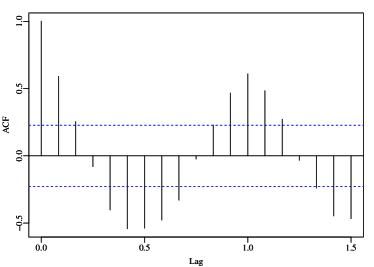
(c) Sampling ACF

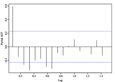
(d) Sampling PACF

Figure 4: Line chart, seasonal component, and correlograms of the discrete-time signal of the monthly number of rainy days in Recife, Brazil.

Based on the three-stage iterative Box-Jenkins methodology [12], i.e., identification—considering an exhaustive search aiming at minimizing the AIC—estimation, and diagnostic checking, we successfully modeled the employed data using the BBARMA$(0,1)$ model with the sinusoidal covariate given above, and considering the logit link function. We employed comparisons among the forecast values of the proposed BBARMA model, the ARMA model [12], and the Holt-Winters method [26, 59]. The ARMA model is widely used in time series analysis and the Holt-Winters method is a nonparametric approach for discrete-time signal processing. Following the iterative methodology described above, the ARMA$(2,1)$ model and the Holt-Winters additive method were elected to fit the considered data set.

The diagnostic analysis of the fitted model was based on the standardized residual $\epsilon[n]$. Table 3 presents the fit of the selected model and the diagnostic analysis. The $p$-values of the Wald test presented in Table 3 suggest that the estimated parameter $\widehat{\beta}_{1}$ is significant to the model for a probability of false alarm equal to $0.05$. Hence, the null hypothesis in (7) can be rejected, indicating a correct detection of the season component. Additionally, the residuals of the fitted model do not exhibit conditional heteroscedasticity or autocorrelation, indicating that the fitted model can be safely used for out-of-signal forecasting.

Table 3: BBARMA$(0,1$) model adjusted for the monthly number of rainy days in Recife, Brazil, considering $H=12$

	${\zeta}$	${\beta}_{1}$	${\theta}_{1}$	${\varphi}$
Estimator	$0.3555$	$-1.0427$	$0.7470$	$27.3863$
Standard Error	$0.0572$	$0.0815$	$0.4130$	$8.5568$
$p$-value	$<0.001$	$<0.001$	$0.0705$	$0.0014$
Diagnostic analysis
Test				$p$-value
Lagrange Multiplier				$0.3582$
Box-Pierce				$0.1881$
Ljung-Box				$0.1295$

Figure 5(a) shows the observed and predicted values obtained considering the fitted BBARMA model. For instance, Figure 5(b) presents the out-of-signal forecast of the adjusted BBARMA$(0,1)$ model, ARMA$(2,1)$ model, and Holt-Winters method for $H=12$. The observed data and the BBARMA model forecasting are discrete values and are represented by line segments between pairs of points. The ARMA model and Holt-Winters out-of-signal forecasts are real numbers whose values are joined with lines segments. In order to have a meaningful comparison of the predicted values, we computed some goodness-of-fit measures, such as root mean squared error (RMSE), median absolute error (MdAE), and mean absolute scaled error (MASE); such measures are expected to be as close to zero as possible [27]. As shown in Table 4, the proposed model outperforms the ARMA model and Holt-Winters method according to the considered figures of merit in both evaluated forecast horizon.

(a) Observed and predicted values

(b) Out-of-signal forecast

Figure 5: Fitted values and out-of-signal forecast of the fiited BBARMA$(1,0)$ model for $H=12$.

Table 4: Forecasting performance comparison among the BBARMA model, ARMA model, and Holt-Winters method. Best results are highlighted

	RMSE	MdAE	MASE
$H=12$
BBARMA	8.5196	5.5000	1.2170
ARMA	$8.9069$	$7.7899$	$1.4098$
Holt-Winters	$9.0478$	$7.0965$	$1.5235$
$H=15$
BBARMA	6.1319	2.0000	$0.8928$
ARMA	$6.1443$	$2.0945$	0.8747
Holt-Winters	$8.5654$	$6.2937$	$1.4856$

6 Conclusion

In this paper, we derived the BBARMA model and a signal detector based on the asymptotic properties of the discussed model estimators. We introduced an inference approach for the model parameters, diagnostic measures, out-of-signal forecasting, the conditional observed information matrix, and the asymptotic properties of the CMLE. Monte Carlo simulations were used as a tool to evaluate the performance of the CMLE and of the proposed signal detector, indicating the consistency of the CMLE. The proposed BBARMA detector could outperform the ARMA- and Gaussian-based detectors in the evaluated scenarios. The proposed model is presented as a suitable tool for quantized signal detection. Additionally, an experiment of the derived BBARMA model considering the monthly number of rainy days in Recife, Brazil, is presented and discussed. The BBARMA model detected the component seasonal in the data set and presented more accurate forecasting results than the traditional ARMA model and Holt-Winters method.

References

- [1] M. Abramowitz and I. A. Stegun, Handbook of Mathematical Functions with Formulas, Graphs, and Mathematical Tables, vol. 9, Dover, New York, 1972.
- [2] H. Akaike, A new look at the statistical model identification, IEEE Transactions on Automatic Control, 19 (1974), pp. 716–723.
- [3] A. Al-Smadi and A. Alshamali, Fitting ARMA models to linear non-Gaussian processes using higher order statistics, Signal Processing, 82 (2002), pp. 1789–1793.
- [4] O. Y. E. Albarracin, A. P. Alencar, and L. Lee Ho, CUSUM chart to monitor autocorrelated counts using negative binomial GARMA model, Statistical Methods in Medical Research, 27 (2018), pp. 2859–2871.
- [5] R. L. Anderson, Distribution of the serial correlation coefficient, The Annals of Mathematical Statistics, 13 (1942), pp. 1–13.
- [6] C. F. Ansley and P. Newbold, Finite sample properties of estimators for autorregressive moving average models, Journal of Econometrics, 13 (1980), pp. 159–183.
- [7] F. M. Bayer, D. M. Bayer, and G. Pumi, Kumaraswamy autoregressive moving average models for double bounded environmental data, Journal of Hydrology, 555 (2017), pp. 385–396.
- [8] BDMEP, Banco de dados meteorológicos para ensino e pesquisa, 2020.
- [9] M. A. Benjamin, R. A. Rigby, and D. M. Stasinopoulos, Generalized autoregressive moving average models, Journal of the American Statistical Association, 98 (2003), pp. 214–223.
- [10] B. M. Bibby and M. Væth, The two-dimensional beta binomial distribution, Statistics & Probability Letters, 81 (2011), pp. 884–891.
- [11] P. Bloomfield, Fourier Analysis of Time Series: An Introduction, John Wiley & Sons, USA, 2004.
- [12] G. Box, G. M. Jenkins, and G. Reinsel, Time Series Analysis: Forecasting and Control, Hardcover, John Wiley & Sons, USA, June 2008.
- [13] G. E. P. Box and D. A. Pierce, Distribution of residual autocorrelations in autoregressive-integrated moving average time series models, Journal of the American Statistical Association, 65 (1970), pp. 1509–1526.
- [14] P. J. Brockwell and R. A. Davis, Time Series: Theory and Methods, Springer Science & Business Media, New York, USA, 2013.
- [15] , Introduction to Time Series and Forecasting, Springer, Switzerland, 2016.
- [16] G. Casella, C. P. Robert, and M. T. Wells, Generalized Accept-Reject Sampling Schemes, Lecture Notes-Monograph Series, (2004), pp. 342–347.
- [17] F. Cribari-Neto and A. Zeileis, Beta regression in R, Journal of Statistical Software, 34 (2010), pp. 1–24.
- [18] B. Efron and D. V. Hinkley, Assessing the accuracy of the maximum likelihood estimator: Observed versus expected Fisher information, Biometrika, 65 (1978), pp. 457–483.
- [19] N. Ehelepola, K. Ariyaratne, W. Buddhadasa, S. Ratnayake, and M. Wickramasinghe, A study of the correlation between dengue and weather in Kandy City, Sri Lanka (2003-2012) and lessons learned, Infectious Diseases of Poverty, 4 (2015), p. 42.
- [20] R. F. Engle, Autoregressive conditional heteroskedasticity with estimates of the variance of UK inflation, Econometrica, 50 (1982), pp. 987–1007.
- [21] S. L. P. Ferrari and E. C. Pinheiro, Improved likelihood inference in beta regression, Journal of Statistical Computation and Simulation, 81 (2011), pp. 431–443.
- [22] A. Forcina and L. Franconi, Regression analysis with the beta-binomial distribution, Rivista di Statistica Applicata, 21 (1988).
- [23] S. Gouveia, T. A. Möller, C. H. Weiß, and M. G. Scotto, A full ARMA model for counts with bounded support and its application to rainy-days time series, Stochastic Environmental Research and Risk Assessment, 32 (2018), pp. 2495–2514.
- [24] E. J. Hannan and B. G. Quinn, The determination of the order of an autoregression, Journal of the Royal Statistical Society. Series B (Methodological), 41 (1979), pp. 190–195.
- [25] R. M. Hirsch and J. R. Slack, A nonparametric trend test for seasonal data with serial dependence, Water Resources Research, 20 (1984), pp. 727–732.
- [26] C. C. Holt, Forecasting seasonals and trends by exponentially weighted moving averages, International Journal of Forecasting, 20 (2004), pp. 5–10.
- [27] R. J. Hyndman and A. B. Koehler, Another look at measures of forecast accuracy, International Journal of Forecasting, 22 (2006), pp. 679–688.
- [28] L. Jacques, D. K. Hammond, and J. M. Fadili, Dequantizing compressed sensing: When oversampling and non-Gaussian constraints combine, IEEE Transactions on Information Theory, 57 (2010), pp. 559–571.
- [29] S. M. Kay, Fundamentals of Statistical Signal Processing: Estimation Theory, Prentice Hall PTR, Upper Saddle River, NJ, USA, 1993.
- [30] S. M. Kay, Fundamentals of Statistical Signal Processing: Detection Theory, vol. II, Prentice Hall, Upper Saddle River, NJ, USA, 1998.
- [31] B. Kedem and K. Fokianos, Regression Models for Time Series Analysis, John Wiley & Sons, New Jersey, USA, 2005.
- [32] R. Koenker and J. Yoon, Parametric links for binary choice models: A Fisherian-Bayesian colloquy, Journal of Econometrics, 152 (2009), pp. 120–130.
- [33] G. Lacombe and M. McCartney, Uncovering consistencies in Indian rainfall trends observed over the last half century, Climatic Change, 123 (2014), pp. 287–299.
- [34] J. C. Lee and J. S. Darius, Bayesian estimation and prediction for the beta-binomial model, Journal of Business & Economic Statistics, 5 (1987), pp. 357–367.
- [35] J. Liu, S. Liu, W. Liu, S. Zhou, S. Zhu, and Z.-J. Zhang, Persymmetric adaptive detection of distributed targets in compound-Gaussian sea clutter with Gamma texture, Signal Processing, 152 (2018), pp. 340–349.
- [36] G. M. Ljung and G. E. P. Box, On a measure of a lack of fit in time series models, Biometrika, 65 (1978), pp. 297–303.
- [37] P. McCullagh and J. Nelder, Generalized Linear Models, Chapman and Hall, New York, USA, 2nd ed., 1989.
- [38] C. E. Metz, Basic principles of ROC analysis, in Seminars in Nuclear Medicine, vol. 8, Elsevier, 1978, pp. 283–298.
- [39] A. N. Njike, R. Pellerin, and J. P. Kenne, Simultaneous control of maintenance and production rates of a manufacturing system with defective products, Journal of Intelligent Manufacturing, 23 (2012), pp. 323–332.
- [40] J. Nocedal and S. J. Wright, Numerical Optimization, Springer, New York, USA, 1999.
- [41] A. V. Oppenheim and R. W. Schafer, Discrete-time Signal Processing, Prentice-Hall Signal Processing Series, Pearson, Upper Saddle River, third ed., 2010.
- [42] B. G. Palm and F. M. Bayer, Bootstrap-based inferential improvements in beta autoregressive moving average model, Communications in Statistics-Simulation and Computation, 47 (2018), pp. 977–996.
- [43] Y. Pawitan, In all Likelihood: Statistical Modelling and Inference Using Likelihood, Oxford Science publications, UK, 2001.
- [44] E. S. Pearson, Bayes’ theorem, examined in the light of experimental sampling, Biometrika, 17 (1925), pp. 388–442.
- [45] W. Press, S. Teukolsky, W. Vetterling, and B. Flannery, Numerical Recipes in C: The Art of Scientific Computing, Cambridge University Press, New York, USA, 2nd edition ed., 1992.
- [46] L. R. Rabiner and R. W. Schafer, Introduction to digital speech processing, Foundations and Trends® in Signal Processing, 1 (2007), pp. 1–194.
- [47] A. V. Rocha and F. Cribari-Neto, Beta autoregressive moving average models, Test, 18 (2009), pp. 529–545.
- [48] A. V. Rocha and F. Cribari-Neto, Erratum to: Beta autoregressive moving average models, Test, 26 (2017), pp. 451–459.
- [49] S. C. Schwartz, J. B. Thomas, and E. J. Wegman, Topics in Non-Gaussian Signal Processing, Springer, New York, USA, 1989.
- [50] G. Schwarz et al., Estimating the dimension of a model, The Annals of Statistics, 6 (1978), pp. 461–464.
- [51] I. G. Skellam, A probability distribution derived from the binomial distribution by regarding the probability of success as variable between the sets of trials, Journal of the Royal Statistical Society. Series B (Methodological), B (1948), pp. 257–261.
- [52] D. M. Stasinopoulos, R. A. Rigby, et al., Generalized additive models for location scale and shape (GAMLSS) in R, Journal of Statistical Software, 23 (2007), pp. 1–46.
- [53] D. Tian, C. J. Martinez, and T. Asefa, Improving short-term urban water demand forecasts with reforecast analog ensembles, Journal of Water Resources Planning and Management, 142 (2016), p. 04016008.
- [54] J. Verbesselt, R. Hyndman, G. Newnham, and D. Culvenor, Detecting trend and seasonal changes in satellite image time series, Remote Sensing of Environment, 114 (2010), pp. 106–115.
- [55] G. Wang, C. Lopez-Molina, G. V.-D. de Ulzurrun, and B. De Baets, Noise-robust line detection using normalized and adaptive second-order anisotropic Gaussian kernels, Signal Processing, 160 (2019), pp. 252–262.
- [56] G. Wang, J. Zhu, R. S. Blum, P. Willett, S. Marano, V. Matta, and P. Braca, Signal amplitude estimation and detection from unlabeled binary quantized samples, IEEE Transactions on Signal Processing, 66 (2018), pp. 4291–4303.
- [57] G. Wang, J. Zhu, and Z. Xu, Asymptotically optimal one-bit quantizer design for weak-signal detection in generalized Gaussian noise and lossy binary communication channel, Signal Processing, 154 (2019), pp. 207–216.
- [58] G. Á. Werner and L. Hanka, Using the beta-binomial distribution for the analysis of biometric identification, in IEEE International Symposium on Intelligent Systems and Informatics, 2015, pp. 209–215.
- [59] P. R. Winters, Forecasting sales by exponentially weighted moving averages, Management Science, 6 (1960), pp. 324–342.