Boundary logarithmic corrections to the dynamical correlation functions of one-dimensional spin-$1/2$ chains

Abstract

The asymptotic dynamical correlation functions in one-dimensional spin chains are described by power-laws. The corresponding exponents characterize different bulk and boundary critical behavior. We present novel results for the logarithmic contribution to the boundary correlations of an isotropic Heisenberg chain. The exponent of the logarithm, $\lambda=1$, is derived using a renormalization group technique. We confirm our analytical results by comparing with numerical quantum Monte Carlo data.

I Introduction

The isotropic spin-$1/2$ chain is one of the most prominent examples of a quantum many-body system. It is fair to say that the one-dimensional Heisenberg model has been an inspiration for fruitful theoretical developments for exact methods, bosonization, and numerical algorithms, ever since the invention of the Bethe ansatz in the early days of quantum mechanics [1]. Critical exponents for spin-spin power-law correlations were first predicted by Luther and Peschel [2] in 1975, which agreed with the pioneering numerical results of Bonner and Fisher [3] from 1964. In 1989, it was realized that the marginally irrelevant “spin-Umklapp” operator leads to multiplicative corrections, with logarithmically increasing behavior in the asymptotic long-distance limit, and is of the form [4, 5, 6, 7]

$$G_{zz}(x,y,t) =\langle S^{z}(x,t)S^{z}(y,0)\rangle$$

$$={\rm const.}\ (-1)^{x-y}\,\frac{\sqrt{\ln r/r_{0}}}{r}\,,$$ (1)

where $r=\sqrt{(x-y)^{2}-v^{2}t^{2}}$ is the space-time distance. This was also confirmed numerically in real space [8, 9]. In a similar calculation, the logarithmic corrections to the dimer correlations, due to the marginally irrelevant operator, were studied, and the asymptotic form of the correlation function was obtained [10, 11].

The focus of this paper is the corresponding logarithmic correction of the boundary critical behavior. Boundaries play an important role in one-dimensional systems. This is due to the fact that for an antiferromagnetic spin chain impurities will effectively cut the chain at low temperatures [12], resulting in zero electric [13] and magnetic conductance [14]. Antiferromagnetic exchange anisotropies correspond to repulsive interactions in fermionic models. Reflecting boundaries induce Friedel oscillations [15, 16, 17, 18, 19] and characteristic boundary correlations [20] which have a large impact on the local density of states in fermionic systems [21, 22, 23, 24, 25] as well as the dynamical structure factor in doped spin chains [26]. Boundary thermodynamics for spin chains and the local susceptibility have been investigated earlier using field theory techniques [27, 28, 29, 30, 31, 32] and the quantum transfer matrix methods [33, 34, 35]. Here, we focus on the spin-spin correlation function for an isotropic chain, which has a different power-law behavior at the boundary [14, 36, 37], viz.

$$G_{zz}(x=y=d,t)={\rm const.\ }\frac{(\ln t/t_{0})^{\lambda}}{t^{2}}\,,$$ (2)

for spins close to a boundary (i.e., where $x=y$ are of the order of the lattice spacing $d$). The exponent $\lambda$ of the logarithm was first predicted to be $\lambda=4$ in a preprint [38], but in subsequent works, $\lambda=2$ has been reported [37, 36]. Ref. [36] uses non-abelian bosonization, while the result of Ref. [37] has been derived implementing abelian bosonization. In our paper, we argue that the exponent is $\lambda=1$ using abelian bosonization, and we also present numerical data based on quantum Monte Carlo simulations to support our analytical results.

II Model and algebraic decay

Before discussing the multiplicative logarithmic corrections, we first briefly summarize the form of the correlations described by the algebraically decaying power-laws, both in the bulk and near the boundaries.

The Hamiltonian of the anisotropic Heisenberg chain in terms of spin-$1/2$ operators $\mathbf{S}_{i}=(S^{x}_{i},S^{y}_{i},S^{z}_{i})$ at site $i$ reads

$$H=J\sum_{i=1}^{L-1}\left(S_{i}^{x}S_{i+1}^{x}+S_{i}^{y}S_{i+1}^{y}+\Delta S_{i}^{z}S_{i+1}^{z}\right),$$ (3)

where $\Delta$ is the anisotropy parameter, and $L$ is the size of the system. Here, we consider “open” boundary conditions, i.e., the edge spins at $i=1$ and $i=L$ are not coupled with each other. For $\Delta=1$, the Hamiltonian is invariant under SU(2) transformations, which is the parameter regime that we will consider in the subsequent discussions. For a more general description, we will use abelian bosonization [39, 40, 41], as the mode expansion is known in this language, thus allowing an explicit calculation of the algebraically-decaying boundary correlation functions [22]. The SU(2) symmetry will be strictly maintained by enforcing the equality of the correlation functions for the transverse and longitudinal directions.

The low-energy effective bosonic description of the anisotropic Heisenberg chain is the Luttinger liquid Hamiltonian [39, 40, 41]

$$H=\frac{\upsilon}{2}\int_{0}^{L}dx \left[K\left(\partial_{x}\tilde{\theta}\right)^{2}+\frac{1}{K}\left(\partial_{x}\tilde{\phi}\right)^{2}\right],$$ (4)

where $\tilde{\phi}$ is the bosonic field, and $\partial_{x}\tilde{\theta}$ is its conjugate momentum, such that $[\tilde{\phi}(x),\partial_{x}\tilde{\theta}(y)]=i\,\delta(x-y)$. The spin-wave velocity $v=J\,\pi\sin\vartheta/2\vartheta$, and the Luttinger parameter $K=\pi/2(\pi-\vartheta)$ are known analytically as functions of $\cos\vartheta=\Delta$, from the exact solution of the model [41]. In our notation, $K=1/2$ corresponds to the SU(2)-invariant point $\Delta=1$. The Luttinger parameter $K$ controls the decay of the correlation functions. It can be gauged away by the canonical transformation

$$\phi=\tilde{\phi}/\sqrt{K},\quad\theta=\sqrt{K}\,\tilde{\theta}\,,$$ (5)

which maps the above Hamiltonian onto a free boson Hamiltonian

$$H_{0}=\frac{v}{2}\int_{0}^{L}dx\left[\left(\partial_{x}\theta\right)^{2}+\left(\partial_{x}\phi\right)^{2}\right].$$ (6)

So far we have omitted the spin-Umklapp operator, which will be discussed in the following section.

Algebraic correlation functions can be determined using the mode expansion (see also the Appendix A) [41, 42]. The overall prefactor of the correlation functions depends on the choice of cutoff in the field theory, but for the spin model it can be fixed using exact methods [43]. For the field theory, it is useful to set the normalization such that in the thermodynamic limit $L\to\infty$, the two-point function of the vertex operator $e^{i\,\gamma\phi}$ (far from the boundary) has the form

$$\langle e^{i\gamma\phi(x,\tau)}\,e^{-i\gamma\phi(y,0)}\rangle=\frac{1}{\left[\,r(x-y,\tau)\,\right]^{2d_{s}}}\,,$$ (7)

for imaginary time $\tau=i\,t$. Here, $d_{s}=\frac{\gamma^{2}}{4\pi}$ is the scaling dimension of the operator, and we introduced

$$r(x,\tau) =\sqrt{x^{2}+v^{2}\,\tau^{2}}$$ (8)

which denotes the space-time distance.

In the following, we are interested in the dominant antiferromagnetic correlations, which arise from the alternating parts of the spin operators in the bosonized form, given by

$$S^{z}(x,t) =A\,(-1)^{x}\sin\left(\sqrt{4\,\pi\,K}\,\phi(x,t)\right),$$ (9)

$$S^{+}(x,t) =\tilde{A}\,(-1)^{x}\,e^{-i\,\sqrt{\frac{\pi}{K}}\,\theta(x,t)},$$ (10)

where $A$ and $\tilde{A}$ are related to the amplitudes of the asymptotic correlation functions [43]. We are now in a position to calculate the longitudinal correlation function $G_{zz}(x,y,\tau)$ [cf. Eq. (I)], and the transverse correlation function

$$G_{+-}(x,y,\tau)=\langle S^{+}(x,\tau)\,S^{-}(y,0)\rangle/2\,.$$ (11)

At the SU(2)-invariant point, the two correlation functions coincide, viz. $G_{zz}=G_{+-}$.

Since we are interested in correlations near boundaries, we evaluate the expectation values using a finite-size bosonization approach, where the mode expansions of the bosonic fields are chosen such that the open boundary conditions of the system are fulfilled. More details are provided in the Appendices B and C. Once the finite-size results are known, these can be generalized to a semi-infinite system with size $L\to\infty$, and with a boundary as $x\to 0$. We find [14, 26] that

$$G_{zz}(x,y,\tau)$$

$$=\frac{A^{2}(-1)^{x+y}}{2\left(4\,x\,y\right)^{K}}\left[\left\{\frac{r(x+y,\tau)}{r(x-y,\tau)}\right\}^{2K}-\left\{\frac{r(x-y,\tau)}{r(x+y,\tau)}\right\}^{2K}\right]$$ (12)

$$\simeq\frac{A^{2}}{2}(-1)^{x+y}\times\begin{cases}r^{-2K}&\text{ bulk }\\ \frac{\left(4\,x\,y\right)^{1-K}}{v^{2}\tau^{2}}&\text{ boundary }\end{cases},$$ (13)

for the Luttinger liquid Hamiltonian in Eq. (4). The bulk limit refers to $x\,y\gg(x-y)^{2}+v^{2}\,\tau^{2}$, while the boundary limit implies $x,\,y\ll v\,t$. We have used $r\equiv r(x-y,\tau)$ without arguments to simplify notation.

An analogous calculation for the transverse correlation function yields

$$G_{+-}(x,y,\tau)$$

$$=\frac{\tilde{A}^{2}}{2}(-1)^{x+y}\left(\frac{4\,x\,y}{r^{2}(x+y,\tau)\,r^{2}(x-y,\tau)}\right)^{\frac{1}{4K}}$$ (14)

$$\simeq\frac{\tilde{A}^{2}}{2}(-1)^{x+y}\,\begin{cases}r^{-\frac{1}{2K}}&\text{ bulk}\\ \left(\frac{4\,x\,y}{v^{4}\,\tau^{4}}\right)^{\frac{1}{4K}}&\text{ boundary}\end{cases}.$$ (15)

At the SU(2)-invariant point, the normalization factors $A$ and $\tilde{A}$ diverge [43], which is the first indication that the prefactors also become dependent on the distance. Nonetheless, for later convenience, we ignore the overall normalization and introduce the short notation $G^{0}(x,y,\tau)$ for the power-law correlation functions at the isotropic point with $K=1/2$. The corresponding asymptotic power-law decays in the two limits follow directly from Eqs. (13) and (15) as

$$G^{0}(x,y,\tau) \propto(-1)^{x+y}\times\begin{cases}r^{-1}&\text{ bulk}\\ \frac{2\sqrt{x\,y}}{v^{2}\,\tau^{2}}&\text{ boundary}\end{cases}.$$ (16)

III Renormalization group flow

Multiplicative logarithmic corrections from the spin-Umklapp operator were first derived using non-abelian bosonization [4] and also using abelian bosonization [5, 6], as two independent approaches. The second approach is the one we will use here for the boundary case. The spin-Umklapp operator is of the form $\cos\left(\sqrt{16\,\pi\,K}\,\phi\right)$. Its scaling dimension $d_{s}=4\,K$ changes continuously with $K$. In particular, at $K=1/2$, the operator is marginal – hence the corrections from a renormalization group (RG) approach are only logarithmically small at best, and must therefore be treated with great care. For this purpose, we will expand the Hamiltonian in Eq. (4) around the SU(2)-invariant point with $K=1/2$. Using the notation $K=1/2+\delta K$ and subsequently rescaling the fields according to Eq. (5) we get

$$H=H_{0}+\int_{0}^{L}dx\left[\,g_{1}\,\mathcal{O}_{1}(x)+g_{2}\,\mathcal{O}_{2}(x)\,\right]$$ (17)

with

$$\mathcal{O}_{1} =\frac{v}{4}\left[\left(\partial_{x}\theta\right)^{2}-\left(\partial_{x}\phi\right)^{2}\right],\,\,\mathcal{O}_{2}=\frac{v}{2\,\pi}\cos\left(\sqrt{8\,\pi}\,\phi\right),$$ (18)

and $g_{1}=4\,\delta K$, while $g_{2}$ is the coupling constant of the spin-Umklapp operator. The value of $g_{2}$ relies on the chosen normalization of the bosonic vertex operators, which in our case is the field theory normalization in Eq. (7). This Hamiltonian defines the starting point of our analysis. The aim of this section is to explain the RG technique to treat the perturbing $\cos\left(\sqrt{8\,\pi\,}{\phi}\right)$ operator in abelian bosonization. We will first revisit the mechanism how the logarithmic corrections to the correlation functions at the SU(2)-invariant point are derived in the bulk limit. We will then employ this analysis to a system with open boundary conditions.

The behavior of the bulk theory under renormalization is well-known. The RG flow equations, which describe how the couplings $g_{1}$ and $g_{2}$ evolve under a change of the length scale $\Lambda$, are of the Kosterlitz-Thouless type [44, 45, 5]. The dependence of the coupling constants on the relevant length scale is encoded in their derivatives with respect to the logarithm of the scale, which, for historical reasons are called beta-functions. In our notation, these read

$$\frac{dg_{2}}{dl}=-{g_{1}\,g_{2}}\,,\quad\frac{dg_{1}}{dl}=-g_{2}^{2}\,,$$ (19)

where $l=\ln(\Lambda/\alpha_{0})$. The parameter $\Lambda$ denotes the physical length scale at which the system is studied, i.e., the corresponding energy scale serves as the infrared cutoff. The ultraviolet energy cutoff corresponds to the length scale $\alpha_{0}$, which has been estimated to be slightly smaller than the lattice spacing $d$, i.e., $\alpha_{0}\approx 0.85\,d$ [9]. The SU(2)-invariant point corresponds to

$$g_{1}=g_{2}=g\,,$$ (20)

where the two beta-functions coincide. Eq. (19) can be exactly solved, and for the isotropic point, the solution is given by

$$g(l) =\frac{g_{0}}{1+b\,g_{0}\,\ln\left(\Lambda/\alpha_{0}\right)}\,.$$ (21)

Here, $b=1$ and $g_{0}$ is the bare coupling, when $\Lambda$ is of the order of $\alpha_{0}$.

In order to derive the logarithmic corrections to the correlation functions, we will follow the approach of Refs. [5, 6]. The multiplicative corrections to the unperturbed correlation function are captured by a function $F_{\mu\nu}(x,y,\tau)$, which is defined by the equation

$$G_{\mu\nu}(x,y,\tau)=G^{0}(x,y,\tau)\,F_{\mu\nu}(x,y,\tau)\,,$$ (22)

where the subscript $\mu\nu$ is the label for the “$zz$” or the “$+-$” components of the correlations. Along the entire line $g_{1}=g_{2}=g$ isotropy must hold [thus implying $F_{zz}(x,y,\tau)=F_{+-}(x,y,\tau)$], and for vanishing $g_{1}=g_{2}=0$ the multiplicative function must be equivalent to the identity [thus implying $F_{\mu\nu}(x,y,\tau)=1$]. The factor $F_{\mu\nu}$ can be derived from the leading-order corrections of the perturbation theory. Here we use the interaction representation [46] and the imaginary time $\tau=i\,t$. The first-order perturbative correction in $g_{1}$ and $g_{2}$ then reads [46]

$$G_{\mu\nu}(x,y,\tau)= G^{0}(x,y,\tau)+\sum_{i=1}^{2}{\mathcal{T}}_{\mathcal{O}_{i}}^{\mu\nu}(x,y,\tau)\,,$$ (23)

where

$${\mathcal{T}}_{\mathcal{O}_{i}}^{\mu\nu}(x,y,\tau)$$

$$=-g_{i}f_{\mu\nu}\int_{0}^{\infty}d\tilde{x}\int_{-\infty}^{\infty}d\tilde{\tau}\Big{\langle}{T}\,S^{\mu}(x,\tau)S^{\nu}(y,0)\mathcal{O}_{i}(\tilde{x},\tilde{\tau})\Big{\rangle}\,$$

$$+g_{i}\,G^{0}(x,y,\tau)\int_{0}^{\infty}d\tilde{x}\int_{-\infty}^{\infty}d\tilde{\tau}\Big{\langle}\mathcal{O}_{i}(\tilde{x},\tilde{\tau})\Big{\rangle}.$$ (24)

with $f_{zz}=1$ and $f_{+-}=\frac{1}{2}$. The symbol ${T}$ in the expectation value denotes the time-ordering operator. In the above expression, the time integral is part of the interaction representation, while the interaction Hamiltonian itself is an integral over the space variable (where we have set the upper boundary $L\to\infty$, valid for a semi-infinite system). The second term in Eq. (24) represents the disconnected diagrams, which we subtract off in order to cancel the unphysical singular contributions. In the next section, we will discuss the expectation values of ${\mathcal{T}}_{\mathcal{O}_{1}}^{\mu\nu}$ and ${\mathcal{T}}_{\mathcal{O}_{2}}^{\mu\nu}$ for open boundary conditions, and evaluate the integrals under a change of cutoff. Combined with the knowledge of the relation between the bare and renormalized couplings, this will determine the factor $F_{\mu\nu}$.

We will illustrate the renormalization of the correlation functions, and how a multiplicative factor $F_{\mu\nu}$ emerges considering the bulk case. Here, $F_{\mu\nu}=F_{\mu\nu}(r/\alpha_{0})$ [cf. Eq. (22)] is a function of the ratio $r/\alpha_{0}$ only. The explicit calculations of ${\mathcal{T}}_{\mathcal{O}_{1}}^{\mu\nu}$ and ${\mathcal{T}}_{\mathcal{O}_{2}}^{\mu\nu}$ (demonstrated in the next section) will show that the integrals, which determine the perturbed correlation function in Eq. (24), exhibit diverging parts around singular points. The latter need to be regularized by the cutoff $\alpha_{0}$. The integrands take the general form

$$f(\tilde{x},\tilde{\tau},x,y,\tau)\Bigg{/}\left[\prod_{s}r^{2}(\tilde{{\bf r}}-{\bf r}_{s})\right],$$ (25)

where $\tilde{{\bf r}}=(\tilde{x},\tilde{\tau})$ is the variable of integration, ${\bf r}_{s}=(x_{s},\tau_{s})$ denotes a singular point, and $f(\tilde{x},\tilde{\tau},x,y,\tau)$ is a polynomial function [cf. Eq. (36), shown in the later part of the paper]. In the bulk limit, the integral structure further simplifies to involve only two singularities at ${\bf r}_{1}=(x,\tau)$ and ${\bf r}_{2}=(y,0)$. The elementary integral that needs to be solved is given by [6]

$$I=\iint^{\prime}d\tilde{x}\,d\tilde{\tau}\frac{1}{r^{2}(\tilde{{\bf r}}-{\bf r}_{1})\,r^{2}(\tilde{{\bf r}}-{\bf r}_{2})}\,.$$ (26)

We regularize the two-dimensional integral by excluding circles of radii $\alpha_{0}$ around ${\bf r}_{1}$ and ${\bf r}_{2}$ while performing the integrations, which is indicated by the symbol $\iint^{\prime}$. While carrying out the integrations, we choose the spatial coordinate axis to be along ${\bf r}_{1}-{\bf r}_{2}$. In the polar coordinates, the integral can then be evaluated

$$I =\int^{{}^{\prime}}d\tilde{r}\int_{0}^{2\pi}d\theta\,\frac{1}{\tilde{r}\left(\tilde{r}^{2}-2\,\tilde{r}\,r\cos\theta+r^{2}\right)}$$

$$=\frac{4\,\pi}{r^{2}}\ln\left(\frac{\Lambda}{\alpha_{0}}\right),$$ (27)

where we have subtracted the singularities within radii $\alpha_{0}\ll r$ around ${\bf r}_{1}$ and ${\bf r}_{2}$, after doing the angular integration exactly. Here, $\Lambda\approx r/\sqrt{2}$ is given in terms of the distance $r=r(x-y,\tau)$ between the two singular points. Note that the distance $r$ serves as the infrared cutoff $\Lambda$ of the integral, because the integrand decays as $1/\tilde{r}^{3}$ for $\tilde{r}\gg r$. In the following, the upper cutoff of the RG procedure is therefore always limited by $r$, which determines the end-point of the logarithmic RG behavior. Hence, each singularity contributes a term $2\,\pi\ln\left(\frac{\Lambda}{\alpha_{0}}\right)$ times the remaining integrand. This logarithm gives a small correction to the correlation function, as long as $\Lambda/\alpha_{0}\sim 1$. In this case, the perturbed correlation function can be generally written as

$$G_{\mu\nu}=G^{0}\left[1+\left(a_{1}\,g_{1}+a_{2}\,g_{2}\right)\ln\left(\frac{\Lambda}{\alpha_{0}}\right)\right],$$ (28)

where $g_{1}=g_{2}=g(l)$, and $a_{1}$ and $a_{2}$ are constants resulting from the perturbative contributions of $\mathcal{O}_{1}$ and $\mathcal{O}_{2}$, respectively. With increasing $\Lambda\sim r$, the “corrections” become arbitrarily large, and consequently, the perturbative approach seems to be doomed. On the other hand, Eq. (28) remains correct if we only want to consider a small change in the cutoff $\Lambda\to\Lambda^{\prime}$. Since the underlying field theory is scale-invariant, Eq. (28) can always be used to calculate the perturbative correction corresponding to a small change $dl=\ln\left(\frac{\Lambda^{\prime}}{\Lambda}\right)$ in the values of the cutoff. Of course, the coupling constant $g(l)$ is not scale-invariant, as it depends on the overall value $l=\ln\left(\frac{\Lambda}{\alpha_{0}}\right)$ in Eq. (21), which must be taken into account at each RG step. We therefore take the cutoff $\Lambda$ as a tunable variable, which can be increased step-by-step from an initially small value $\Lambda=\alpha_{0}$, until the physical cutoff $\Lambda\sim r$ is reached. At each step, we use Eq. (28) to calculate the correction of $G_{\mu\nu}$, assuming that $l=\ln\left(\frac{\Lambda}{\alpha_{0}}\right)$ only changes by an infinitesimal amount $dl=\ln\left(\frac{\Lambda^{\prime}}{\Lambda}\right)$, and $g_{1}=g_{2}=g(l)$ is given by the running coupling constants in Eq. (21). To make it more concrete, let us look at the renormalization of $F_{\mu\nu}$ as we slightly increase the cutoff $\Lambda\to\Lambda^{\prime}$ . This is captured by

$$F_{\mu\nu}(\Lambda^{\prime}/\alpha_{0})=F_{\mu\nu}(\Lambda/\alpha_{0})\left[1+a\,g(l)\ln\left(\frac{\Lambda^{\prime}}{\Lambda}\right)\right],$$ (29)

where $a=a_{1}+a_{2}$. Iterating and multiplying all RG steps from $\Lambda=\alpha_{0}$ to $\Lambda=r$, we find that

$$F_{\mu\nu}(r/\alpha_{0}) =\prod_{l=0}^{\ln(r/\alpha_{0})}\left[1+a\,g(l)dl\right]$$

$$=\exp\left[\int_{0}^{\ln(r/\alpha_{0})}\gamma_{\mu\nu}(l)\,dl\right],$$ (30)

where we have introduced

$$\gamma_{\mu\nu}(l)=a\,g(l)\,,$$ (31)

which is twice the commonly defined anomalous dimension of the corresponding spin-field [47]. Notice that the anomalous dimension is defined as the logarithmic derivative of the prefactor, which renormalizes the correlation function multiplicatively under a change of scale [47]. Therefore, it depends on the coupling of the theory at any scale. Finally, making use of Eq. (21), and performing the integral in Eq. (III), we obtain the form of multiplicative logarithmic correction as

$$F_{\mu\nu}(r/\alpha_{0}) =\exp\left\{\frac{a}{b}\ln\left[1+b\,g_{0}\ln(r/\alpha_{0})\right]\right\}$$

$$=\left[1+b\,g_{0}\ln(r/\alpha_{0})\right]^{\frac{a}{b}}\,.$$ (32)

Eq. (32) thus provides a general recipe for the logarithmic correction to any correlation function. It involves two characteristic quantities: (1) the beta-function of the theory which determines the parameter $b$; and (2) the anomalous dimension $\gamma_{\mu\nu}$ of the corresponding spin-field in Eq. (31), which determines the parameter $a$.

Indeed, the concept of the anomalous dimension is well known from the Callan-Symanzik equation, describing the evolution of any $n$-point correlation function under variation of the energy scale [48], which of course gives an identical result [4, 5, 6]. In the case of open boundary conditions, however, the above step-by-step RG treatment appears to be more transparent, because there are two length scales in the boundary theory, viz. $r(x-y,\tau)$ and $r(x+y,\tau)$. We will show that in the bulk and boundary limits, the two length scales reduce again to a single one, viz. $\Lambda=r$ and $\Lambda=v\,t$, respectively. In these cases, the RG treatment is fully analogous to the one described above, with the corresponding length scales taken into account. We will now proceed to explicitly determine the parameters $a$ and $b$ entering Eq. (32), for both the bulk and the boundary limits.

IV First order perturbation

In this section, we discuss the first order corrections to the free correlation function, due to the presence of the operators $\mathcal{O}_{1}$ and $\mathcal{O}_{2}$. We identify the logarithmically divergent pieces of the resulting integrals, in order to obtain the general form of Eq. (28), and to determine the prefactors $a_{1}$ and $a_{2}$. The knowledge of these prefactors is crucial as they enter the final exponent of the multiplicative logarithmic exponent in Eq. (32) where $a=a_{1}+a_{2}$. Our focus will be on the boundary behavior of a semi-infinite chain. For a better understanding, we will also include results for the bulk limit, where we recover the known results for the infinite case.

Let us start by discussing the contribution of the operator $\mathcal{O}_{1}$. In this case, we do not need to evaluate the expectation value in a first order perturbative expression at all, as there is a much simpler way to determine the constant $a_{1}$. The operator $\mathcal{O}_{1}$ can be included in the quadratic part of the Hamiltonian, allowing it to be treated exactly. This just affects the value of the Luttinger parameter, which increases as $K\to K+\delta K$ with $\delta K=g_{1}/4$. Eq. (13) for the correlation function $G_{zz}(x,y,\tau)$ is still valid, using $K=\frac{1}{2}+\delta K$ in the vicinity of the isotropic point. The first order correction ${\mathcal{T}}_{\mathcal{O}_{1}}^{zz}$ can now be obtained by expanding the power-law expression for $G_{zz}(x,y,\tau)$ in $\delta K$, leading to

$${\mathcal{T}}_{\mathcal{O}_{1}}^{zz}=-\frac{g_{1}\,A^{2}\,(-1)^{x+y}}{2}\begin{cases}\frac{1}{2\,r}\ln\left(\frac{\Lambda}{\alpha_{0}}\right)&\text{ bulk}\\ 0&\text{ boundary}\\ \end{cases}.$$ (33)

Here, we have used the fact that the infrared cutoff is given by the distance $\Lambda\sim r$, relative to the ultraviolet cutoff $\alpha_{0}$. Note that in the boundary case, the power $(x\,y)^{1-K}$ appearing in the correlation function in Eq. (13), contributes a logarithm $\sim\ln\left({x\,y}\,/{\alpha_{0}^{2}}\right)$, which vanishes near the boundary $x,y\sim\alpha_{0}$ – hence it has been neglected here.

For the contribution of the operator $\mathcal{O}_{2}$, we need to evaluate the integral corresponding to the first order perturbation explicitly, which is a straightforward but cumbersome calculation. We can express the perturbative change of the correlation function from ${\mathcal{O}_{2}}$ as a sum of the two integrals $I_{1}$ and $I_{2}$, such that

$${\mathcal{T}}_{\mathcal{O}_{2}}^{zz}(x,y,\tau)$$ (34)

$$=-\frac{g_{2}\,v\,A^{2}(-1)^{x+y}}{8\,\pi\,\sqrt{x\,y}}\left[\frac{r(x+y,\tau)}{r(x-y,\tau)}\,{I}_{1}-\frac{r(x-y,\tau)}{r(x+y,\tau)}\,{I}_{2}\right].$$

Here,

$${I}_{i}=\iint^{\prime}d\tilde{x}\,d\tilde{\tau}\,t_{i}(x,y,\tilde{x},\tau,\tilde{\tau})\,,$$ (35)

for $i=1,2$, and the integral therefore denotes the correction due to a small change of the cutoff around each singularity. Each integrand $t_{i}$ is determined from evaluating the time-ordered correlation function in Eq. (24), using the mode expansion shown in the Appendix A. This gives us (for details see Appendix D)

$$t_{1/2}=$$ (36)

$$\left[\frac{(\tilde{\tau}^{2}+\tilde{x}^{2}+y^{2})x\mp((\tau-\tilde{\tau})^{2}+\tilde{x}^{2}+x^{2})y}{r({\tilde{x}}-x,\tilde{\tau}-\tau)\,r({\tilde{x}}+x,\tilde{\tau}-\tau)\,r({\tilde{x}}-y,\tilde{\tau})\,r({\tilde{x}}+y,\tilde{\tau})}\right]^{2}.$$

Since the correlations are symmetric under $\tilde{x}\to-\tilde{x}$, we do not need to restrict the integration to positive values only. In the above expression, the contributions from the disconnected diagrams have already been subtracted. The final integrals are dominated by the behavior of the integrands in the vicinity of the singular points, which determine the leading order logarithmic contributions. For both the terms $t_{1}$ and $t_{2}$, there are four singular points, which are located at $(\tilde{x}\rightarrow\pm x,\,\tilde{\tau}\rightarrow\tau)$, and $(\tilde{x}\rightarrow\pm y,\,\tilde{\tau}\rightarrow 0)$.

We now determine the leading logarithmic contributions to the integrals, by choosing an appropriate parametrization in the vicinity of each singular point. For instance, we choose $(\tilde{x}=x+\delta{\tilde{x}},\,\tilde{\tau}=\tau+\delta\tilde{\tau})$ for the point $(\tilde{x}\rightarrow x,\,\tilde{\tau}\rightarrow\tau)$, and then expand for small $\delta\tilde{x}$ and $\delta\tilde{\tau}$. Analogous to Eq. (27), each singularity contributes $2\,\pi\ln(\Lambda/\alpha_{0})$ times the corresponding value of the remaining integrand, leading to

$$I_{1} \simeq 2\,\pi\left[\frac{r(x-y,\tau)}{r(x+y,\tau)}\right]^{2}\ln\left(\frac{\Lambda}{\alpha_{0}}\right),$$ (37)

$$I_{2} \simeq 2\,\pi\left[\frac{r(x+y,\tau)}{r(x-y,\tau)}\right]^{2}\ln\left(\frac{\Lambda}{\alpha_{0}}\right).$$ (38)

Inserting these results in Eq. (34), we obtain

$${\mathcal{T}}_{\mathcal{O}_{2}}^{zz}$$ (39)

$$=\frac{g_{2}\,A^{2}\,(-1)^{x+y}}{4\,\sqrt{x\,y}}\left[\frac{r(x+y,\tau)}{r(x-y,\tau)}-\frac{r(x-y,\tau)}{r(x+y,\tau)}\right]\ln\left(\frac{\Lambda}{\alpha_{0}}\right)$$

which reduces to

$${\mathcal{T}}_{\mathcal{O}_{2}}^{zz}$$ (40)

$$=\frac{g_{2}\,A^{2}\,(-1)^{x+y}}{2}\begin{cases}\frac{1}{r}\ln\left(\frac{\Lambda}{\alpha_{0}}\right)&\text{ bulk}\\ \frac{2\,\sqrt{x\,y}}{v^{2}\,\tau^{2}}\ln\left(\frac{\Lambda}{\alpha_{0}}\right)&\text{ boundary}\end{cases},$$

in the two limits. Finally, we add ${\mathcal{T}}_{\mathcal{O}_{1}}^{zz}$ in Eq. (33), and ${\mathcal{T}}_{\mathcal{O}_{2}}^{zz}$ in Eq. (40), to the unperturbed correlation function in Eq. (16). This leads to

$$G_{zz}(x,y,\tau)$$ (41)

$$=\frac{A^{2}\,(-1)^{x+y}}{2}\begin{cases}\frac{1}{r}\left[1+\left(g_{2}-\frac{g_{1}}{2}\right)\ln\left(\frac{\Lambda}{\alpha_{0}}\right)\right]&\text{ bulk}\\ \frac{2\sqrt{x\,y}}{v^{2}\,\tau^{2}}\left[1+g_{2}\ln\left(\frac{\Lambda}{\alpha_{0}}\right)\right]&\text{ boundary}\end{cases}.$$

We thus obtain an expression which agrees with the general form shown in Eq. (28), with the coefficients ($a_{1}=-\frac{1}{2},a_{2}=1$, $a=\frac{1}{2}$) in the bulk limit, and ($a_{1}=0$, $a_{2}=1$, $a=1$) in the boundary limit.

We are now in the position to state the final result for the exponent $\lambda=\frac{a}{b}$ of the logarithmic correction, both in the bulk and boundary limits. Using Eq. (41) and Eq. (32), we find that $a=\frac{1}{2}$ and $b=1$ in the bulk limit. This gives us the logarithmically corrected correlation function [4, 5, 6]

$$G(r)=\frac{A^{2}(-1)^{x+y}}{2\,r}\sqrt{\ln\left(r/\alpha_{0}\right)}\,,$$ (42)

with a bulk logarithmic exponent $\lambda={1}/{2}$. In the boundary limit, we find that $a=1$ and $b=1$, which results in the logarithmically corrected correlation function

$$G_{b}(t)=-\frac{A^{2}(-1)^{x+y}\,\sqrt{x\,y}}{v^{2}\,t^{2}}\ln\left(\frac{t}{t_{0}}\right)\,$$ (43)

with a boundary logarithmic exponent $\lambda=1$. This is the main result of this paper, which, however, does not agree with what was obtained earlier [36, 37]. Hence, it warrants a critical discussion about the possible origin of this discrepancy.

V Critical discussion

In this section, we will explain the reasons why we believe that we do not recover the boundary logarithm exponent $\lambda=2$ of previous works [36, 37]. While we have obtained the same beta-functions, and the coefficient $b=1$, we obtain a different anomalous dimension with the coefficient $a=1$ (as opposed to $a=2$, found in earlier works). The discrepancy stems from taking a different order of the calculational steps – in our case, we first evaluate the full integral in Eq. (39), and then take the boundary limit in Eq. (40). In contrast, in the earlier papers [36, 37], where an operator product expansion was employed, the order of calculations amounts to first taking the boundary limit in the correlation function, for small $x,y$. However, when taking the boundary limit, the singularities (appearing at $\tilde{x}=-x$ and $\tilde{x}=x$) get partially reduced due to factors in the numerator, leaving only one singularity instead of two (albeit with a prefactor which is four times larger). Note that this procedure assumes that $x,y\lesssim\alpha_{0}$, and therefore does not capture the diverging dependence on the lower length scale cutoff $\alpha_{0}$ correctly. On the other hand, in our approach, the arguments $(x,y)$ are always larger than the cutoff $\alpha_{0}$, as they must be, judging from physical intuition and the estimate $\alpha_{0}\approx 0.85\,d$ [9]. In the bulk limit, in contrast, the order of the computational steps does not make any difference. In fact, the bulk limit can be safely taken before integrating, as all singularities are always sufficiently removed from each other.

Let us show explicitly that the expansion for small $(x,y)$ as the first step, starting from the same correlation function in Eq. (36), leads to a different result. First expanding ${\mathcal{T}}_{\mathcal{O}_{2}}^{zz}$ in Eq. (34) for small $(x,y)$, before performing the integral, we find that

$${\mathcal{T}}_{\mathcal{O}_{2}}^{zz}(x,y,\tau)$$ (44)

$$= \frac{g_{2}\,v\,A^{2}(-1)^{x+y}}{2\,\pi}\iint^{\prime}d\tilde{x}\,d\tilde{\tau}\frac{\sqrt{x\,y}}{r^{2}(\tilde{x},\tilde{\tau})\,r^{2}(\tilde{x},\tilde{\tau}-\tau)}\,.$$

Here, we have dropped all terms which are odd under parity [viz., $\tilde{x}\to-\tilde{x}$], and which therefore do not contribute to the integral. The integrand is singular for $(\tilde{x}\to 0,\tilde{\tau}\to 0)$ and $(\tilde{x}\to 0,\tilde{\tau}\to\tau)$. Integration in the same manner as before yields

$${\mathcal{T}}_{\mathcal{O}_{2}}^{zz}(x,y,\tau)=g_{2}\,A^{2}(-1)^{x+y}\;\frac{2\sqrt{x\,y}}{v^{2}\,\tau^{2}}\ln\left(\frac{\Lambda}{\alpha_{0}}\right).$$ (45)

Note the additional factor 2 as compared to Eq. (40). This factor leads to an anomalous dimension $a=2$ and as a result the logarithmic exponent $\lambda$ is twice as large as our exponent $\lambda=1$ for the boundary case. Since the analytic structure is changed by taking the limit of small $(x,y)$ first, we do not believe that the previous result of $a=2$ is correct.

A further check of our result comes from the transverse correlation function, which has an identical logarithmic correction. A calculation analogous to the one before for the contribution of the $\mathcal{O}_{1}$ operator, expanding $K=\frac{1}{2}+\delta K$ for small $\delta K$ in the transverse correlation function, gives us

$${\mathcal{T}}_{\mathcal{O}_{1}}^{+-}=\frac{g_{1}\,\tilde{A}^{2}}{2}\,(-1)^{x+y}\times\begin{cases}\frac{1}{2r}\ln\left(\frac{\Lambda}{\alpha_{0}}\right)&\text{ bulk}\\ \frac{2\sqrt{x\,y}}{v^{2}\,\tau^{2}}\ln\left(\frac{\Lambda}{\alpha_{0}}\right)&\text{ boundary}\end{cases}.$$ (46)

For this case, the operator $\mathcal{O}_{2}$ does not generate a logarithmically divergent term in first order in $g_{2}$ as shown in the Appendix E. In other words,

$${\mathcal{T}}_{\mathcal{O}_{2}}^{+-}=0\,.$$ (47)

This calculation confirms once again that $a=1$ in the boundary case, as also required by the rotational invariance. Even though the separate contributions of $a_{1}$ and $a_{2}$ are different for the transverse and longitudinal correlations functions, the sum $a=a_{1}+a_{2}$ is the same. Indeed, we find that along the isotropic line $g_{1}=g_{2}=g$, the logarithmic corrections to the decay of the spin-spin correlation functions follow

$$G_{+-}(x,y,\tau)=\frac{\tilde{A}^{2}}{2}\,(-1)^{x+y}$$ (48)

$$\,\times\begin{cases}\frac{1}{r}\left[1+\frac{g_{1}}{2}\ln\left(\frac{\Lambda}{\alpha_{0}}\right)\right]&\text{bulk}\\ \frac{2\sqrt{x\,y}}{v^{2}\,\tau^{2}}\left[1+g_{1}\ln\left(\frac{\Lambda}{\alpha_{0}}\right)\right]&\text{boundary}\end{cases},$$

and thus

$${\mathcal{T}}_{\mathcal{O}_{1}}^{zz}+{\mathcal{T}}_{\mathcal{O}_{2}}^{zz}={\mathcal{T}}_{\mathcal{O}_{1}}^{+-}+{\mathcal{T}}_{\mathcal{O}_{2}}^{+-}.$$ (49)

VI Numerical data and fits

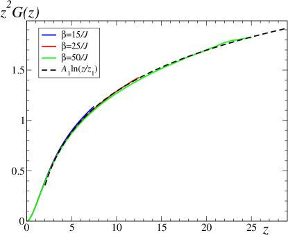
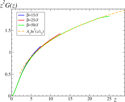
Figure 1: The curves show the data points obtained from the quantum Monte Carlo Simulations for the boundary correlation function $z^{2}\,G_{zz}(z)$ of the last spin in an isotropic chain in imaginary-time as a function of $z=\frac{v\,\beta}{\pi}\sin\left(\frac{\pi\tau}{\beta}\right)$. The three curves correspond to $\beta J=15,25,50$. The fits according to Eq. (51) with the parameter values taken from the last line of the Table 1 are shown for $\lambda=1$ (top) and $\lambda=2$ (bottom).

In order to test the predictions form our analytical calculations, we have performed numerical quantum Monte Carlo simulations, using the Stochastic Series Expansion algorithm [49, 50] with directed loop updates [51] and a Mersenne Twister random number generator [52]. With this method, it is straight-forward to calculate correlation functions in the imaginary time $\tau$ at finite temperatures [49].

Using the mode expansion of the fields, the method to calculate the power-law correlations for any finite size $L$ and finite temperature $T$ is well-known [22, 42, 28]. In particular, for finite temperatures, the imaginary space-time coordinate $i\,x+v\,\tau$ in the correlation functions is replaced by [27]

$$i\,x+v\,\tau\to z=\frac{v\,\beta}{\pi}\sin\Big{(}\frac{\pi\left(i\,x+v\,\tau\right)}{v\,\beta}\Big{)}\,.$$ (50)

Here, it is assumed that the inverse temperature is $\beta=1/T\ll L/v$, such that the effects from the finite system size $L$ can be ignored [22, 42, 28]. It has been argued in Ref. [53] that the RG treatment can also be performed in the variable $z$, up to second order in the beta-function, but that higher order RG may not give a perfect data collapse as a function of $z$. We, therefore, analyze the imaginary-time correlation function of the last spin of an open chain, using the ansatz

$$G_{zz}(x=y=d,\tau)={\rm A_{\lambda}\ }\frac{[\,\ln\left(z/z_{\lambda}\right)\,]^{\lambda}}{z^{2}}\,,$$ (51)

with $z=\frac{v\,\beta}{\pi}\sin\left(\frac{\pi\,\tau}{\beta}\right)$, exponent $\lambda=1,2$, and fitting constants $A_{1,2}$ and $z_{1,2}$. The corresponding quantum Monte Carlo data for an isotropic chain of length $L=500$, at three different temperatures $\beta J=15,25,50$ are shown in Fig. 1, where we have multiplied the correlation function with the leading power-law $z^{2}$. The results for different temperatures have approximately the same functional dependence on $z$, and hence the higher order RG corrections, which are not functions of $z$, can indeed be neglected.

$\beta J$	$A_{1}$	$z_{1}$	$A_{2}$	$z_{2}$
15	0.583235	0.935679	0.104749	3.65832
25	0.584947	0.908307	0.0864403	4.72989
50	0.594767	0.86585	0.070273	6.78464
all	0.58763	0.898285	0.0674096	7.60085

Table 1: Fitting parameters.

The constants $A_{1,2}$ and $z_{1,2}$ have been determined by the best fits to Eq. (51) for $z>2$ and are shown in Table 1. At the first sight, both $\lambda=1$ and $\lambda=2$ appear to fit well with the data. But upon closer inspection, the fit for $\lambda=2$ has clear systematic deviations, as seen in Fig. 1 and Table 1. In particular, the fitting parameters in Table 1 drift as a function of $\beta$ by 30% or more, while the parameters for $\lambda=1$ remain constant for different $\beta$ within a few percent. Notice that it is important to analyze the quality of the fit over the entire range of data for different temperatures. We therefore conclude that the data shows clear evidence that $\lambda=1$ is the correct exponent for the boundary logarithmic corrections.

VII Conclusion

We have considered the boundary logarithmic correction to the dynamical spin-spin correlation function, for the isotropic Heisenberg chain. The logarithmic corrections are caused by the marginal spin-Umklapp operator, which we have treated by RG techniques. When both spins are located close to the open boundary, the correlations are captured by a single scale $\upsilon t$, which allows using scaling arguments analogous to the bulk theory. We have found an anomalous dimension which results in an exponent $\lambda=1$ for the logarithmic correction. This result is confirmed by the state-of-the-art numerical data from quantum Monte Carlo simulations.

The time-dependent spin-spin correlation functions can be probed by the nuclear magnetic resonance (NMR) relaxation rates of spin-$1/2$ antiferromagnetic chain compounds. For the bulk materials, experimental data on Sr₂CuO₃ [54] have been found to be in good agreement with theoretical predictions incorporating multiplicative logarithmic corrections [55, 56]. In addition, impurity effects on the NMR spectra have also been studied [57]. Recently, the magnetic properties of doped spin chains have attracted renewed experimental interest [58, 59]. As the current experimental resolution for NMR data is much better than the numerical capabilities to simulate the behaviour at long times, we believe that a comparison of our results to the boundary NMR relaxation rates [37] will potentially resolve the issue. An alternative (and extremely promising) route is given by experiments on ultracold gases realizing the spin-1/2 Heisenberg chain [60, 61], where measurements of time and space-resolved correlations have been proposed [26, 62, 63]. As these systems always have finite system sizes, precise knowledge of the boundary effects, that we have investigated in our paper, is of great importance.

Appendix A Mode Expansions for the semi-infinite chain

To account for the open boundary condition on the left end of the semi-infinite chain, we impose the Dirichlet boundary condition on the spin field at the boundary $x=0$ [37, 14], which implies that $\left\langle S^{z}(x=0)\right\rangle=0$. By using the expression for the bosonized spin operators [cf. Eq. (9)], where the bosonization field $\phi(x,t)=\phi_{L}(x,t)+\phi_{R}(x,t)$, we obtain $\phi_{0}\equiv\phi(x=0)=k\,\sqrt{\pi/\left(4K\right)}$ (with $k\in\mathbb{Z}$). Since the chiral bosonic fields $\phi_{R}$ and $\phi_{L}$ are functions of $(x-v\,t)$ and $(x+v\,t)$, respectively, the Dirichlet boundary condition allows us to relate them as $\phi_{R}(x,t)=-\phi_{L}(-x,t)+\phi_{0}$. Hence, the mode-expansions for these fields take the form [14, 42]:

$$\phi_{L}(x,t)=\frac{\phi_{0}+\tilde{\phi}_{0}}{2}+\frac{x+v\,t}{2\,L}\,Q+\sum_{\ell>0}\left[\frac{i\,e^{-\frac{i\,\pi\,\ell}{L}(x+v\,t)}}{\sqrt{4\,\pi\,\ell}}\,b_{\ell}+\mathrm{H.c.}\right]\,,$$

$$\phi_{R}(x,t)=\frac{\phi_{0}-\tilde{\phi}_{0}}{2}+\frac{x-v\,t}{2\,L}\,Q+\sum_{\ell>0}\left[-\frac{i\,e^{\frac{i\,\pi\,\ell}{L}(x-v\,t)}}{\sqrt{4\,\pi\,\ell}}\,b_{\ell}+\mathrm{H.c.}\right]\,,$$

$$\phi(x,t)={\phi}_{0}+\frac{x}{L}\,Q+\sum_{\ell>0}\frac{\sin\left(\frac{\pi\,\ell\,x}{L}\right)}{\sqrt{\pi\,\ell}}\left[e^{-\frac{i\,\pi\,\ell\,v\,t}{L}}\,b_{\ell}+\mathrm{H.c.}\right]\,,$$

$$[b_{\ell},\,b_{\ell^{\prime}}^{\dagger}]=\delta_{\ell,\ell^{\prime}}\,,\quad[\tilde{\phi}_{0},\,Q]=i\,.$$ (52)

For the conjugate field $\theta(x,t)=\phi_{L}(x,t)-\phi_{R}(x,t)$ we have

$$\theta(x,t)=\tilde{\phi}_{0}+\frac{v\,t}{L}\,Q+\sum_{\ell>0}\frac{\cos\left(\frac{\pi\,\ell\,x}{L}\right)}{\sqrt{\pi\,\ell}}\left[i\,e^{-\frac{i\,\pi\,\ell\,v\,t}{L}}\,b_{\ell}+\mathrm{H.c.}\right].$$ (53)

Appendix B Unperturbed correlation function $G_{zz}(x,y,t)$

In this section, we will explain how to calculate expectation values in general, using the mode expansion of the previous section. An example of this procedure is given by the evaluation of the unperturbed correlation function $G_{zz}(x,y,t)$.

We start from the bosonized spin operator

$$S^{z}(x,t)=A\,(-1)^{x}\sin\left(\sqrt{4\pi K}\,\phi(x,t)\right),$$ (54)

as shown in Eq. (9). The expectation values in the ground state can be evaluated in the simplest way by normal ordering all the expressions, with respect to the annihilation and creation operators $b_{\ell}$ and $b_{\ell}^{\dagger}$, respectively. Using the Baker-Campbell-Hausdorff formula $e^{A+B}=e^{A}\,e^{B}\,e^{-\frac{1}{2}[A,B]}$ for $\left[A,[A,B]\right]=0$ and $\left[B,[B,A]\right]=0$, we find that, for a general vertex operator [26],

$$e^{i\,\alpha\,\sqrt{4\pi}\,\phi(x,t)} =\left[\frac{\pi}{2\,L\sin\left(\pi\,x/L\right)}\right]^{\alpha^{2}}\exp\left(i\,\alpha\sum_{\ell}e^{i\,\omega_{\ell}\,t}\,\frac{A_{\ell}^{\dagger}(x)}{\sqrt{\ell}}\right)\exp\left(i\,\alpha\sum_{\ell}e^{-i\,\omega_{\ell}\,t}\,\frac{A_{\ell}(x)}{\sqrt{\ell}}\right)$$ (55)

$$=\left[\frac{\pi}{2\,L\sin\left(\pi\,x/L\right)}\right]^{\alpha^{2}}:e^{i\,\alpha\,\sqrt{4\pi}\,\phi(x,t)}:\,,$$ (56)

where $\omega_{\ell}=\frac{\pi v\,\ell}{L}$ and

$$A_{\ell}(x)=2\sin\left(\frac{\ell\,\pi\,x}{L}\right)b_{\ell}\,.$$ (57)

Here, we have used the expansion of the logarithm $\sum_{\ell=1}^{\infty}\frac{e^{-i\omega_{\ell}t}}{\ell}=-\ln\left(1-e^{-\frac{i\pi vt}{L}}\right)$ where we assume that $t$ comes with a small negative imaginary part to ensure convergence. We also have set the normalization of the single vertex operator such that for the two-point function far away from the boundary Eq. (7) is fulfilled. For a product of two vertex operators, we further need to normal order the inner products of the exponentials, in order to obtain a fully normal ordered expression. This yields

$$e^{i\,\alpha\,\sqrt{4\pi}\phi(x,t)}\,e^{i\,\beta\,\sqrt{4\pi}\phi(y,0)}=\frac{\left(\frac{\pi}{2\,L}\right)^{\alpha^{2}+\beta^{2}}e^{-\alpha\,\beta\,C_{1}(x,y,t)}}{\sin^{\alpha^{2}}\left(\frac{\pi\,x}{L}\right)\sin^{\beta^{2}}\left(\frac{\pi\,y}{L}\right)}:e^{i\,\alpha\,\sqrt{4\pi}\phi(x,t)}\,e^{i\,\beta\,\sqrt{4\pi}\phi(y,0)}:\,,$$ (58)

with the commutator

$$C_{1}(x,y,t) =\sum_{\ell,\ell^{\prime}}\frac{e^{-i\,\omega_{\ell}\,t}}{\sqrt{\ell\,\ell^{\prime}}}[A_{\ell}(x),A^{\dagger}_{\ell^{\prime}}(y)]=4\sum_{\ell}\frac{e^{-i\,\omega_{\ell}\,t}}{\ell}\sin\left(\frac{\ell\,\pi x}{L}\right)\sin\left(\frac{\ell\,\pi y}{L}\right)$$ (59)

$$=\Big{[}-\ln\left(1-e^{-\frac{i\pi}{L}(x-y+v\,t)}\right)+\ln\left(1-e^{-\frac{i\pi}{L}(x+y+v\,t)}\right)$$

$$\qquad\quad+\ln\left(1-e^{\frac{i\pi}{L}(x+y-v\,t)}\right)-\ln\left(1-e^{\frac{i\pi}{L}(x-y-v\,t)}\right)\Big{]}$$

$$\simeq\ln\left[\frac{\left(x+y\right)^{2}-(v\,t)^{2}}{\left(x-y\right)^{2}-(v\,t)^{2}}\right].$$ (60)

In the last line, we have taken the limit $L\to\infty$. Thus, we get

$$e^{i\,\alpha\,\sqrt{4\pi}\,\phi(x,t)}\,e^{i\,\beta\,\sqrt{4\pi}\,\phi(y,0)}\simeq\frac{\left[\frac{\left(x+y\right)^{2}-v^{2}\,t^{2}}{\left(x-y\right)^{2}-v^{2}\,t^{2}}\right]^{-\alpha\,\beta}}{(2\,x)^{\alpha^{2}}(2\,y)^{\beta^{2}}}:e^{i\,\alpha\,\sqrt{4\pi}\,\phi(x,t)}\,e^{i\,\beta\,\sqrt{4\pi}\,\phi(y,0)}:\,.$$ (61)

For the correlation function

$$G_{zz}(x,y,t)=A^{2}\,(-1)^{x+y}\left\langle\sin\left(\sqrt{4\pi K}\,\phi(x,t)\right)\sin\left(\sqrt{4\pi K}\,\phi(y,0)\right)\right\rangle,$$ (62)

we need to combine four different products of the vertex operators. Using the above expressions, to leading order, we find that

$$G_{zz}(x,y,t)=\frac{A^{2}\,(-1)^{x+y}}{2\left(4\,x\,y\right)^{K}}\left[\left\{\frac{\left(x+y\right)^{2}-v^{2}\,t^{2}}{\left(x-y\right)^{2}-v^{2}\,t^{2}}\right\}^{K}-\left\{\frac{\left(x-y\right)^{2}-v^{2}\,t^{2}}{\left(x+y\right)^{2}-v^{2}\,t^{2}}\right\}^{K}\right],$$ (63)

which agrees with Eq. (12) after switching to imaginary time (i.e., $t\to-i\,\tau$). In the bulk limit of $x\,y\gg r^{2}$ [where $r^{2}=(x-y)^{2}-v^{2}\,t^{2}$], we obtain

$$G_{zz}(x,y,t)\big{|}_{\text{bulk}} =\frac{A^{2}\,(-1)^{x+y}}{2\left(4\,x\,y\right)^{K}}\left[\left\{\frac{r^{2}+4\,x\,y}{r^{2}}\right\}^{K}-\left\{\frac{r^{2}}{r^{2}+4\,x\,y}\right\}^{K}\right]\simeq\frac{A^{2}(-1)^{x+y}}{2\left(4\,x\,y\right)^{K}}\left[\left(\frac{4\,x\,y}{r^{2}}\right)^{K}-0\right]$$

$$=A^{2}\,(-1)^{x+y}\frac{1}{2\,r^{2K}}\,.$$ (64)

Finally, the boundary limit implies $x,\,y\ll v\,t$, which gives

$$G_{zz}(x,y,t)\big{|}_{\text{boundary}} =-A^{2}\,(-1)^{x+y}\frac{\left(4\,x\,y\right)^{1-K}}{2\,v^{2}\,t^{2}}\,.$$ (65)

Appendix C Unperturbed correlation function $G_{+-}(x,y,t)$

In this section, we consider the spin operator

$$S^{+}(x,t)=\tilde{A}\,(-1)^{x}\,e^{-i\,\sqrt{\frac{\pi}{K}}\,\theta(x,t)}\,,$$ (66)

as shown in Eq. (10), and calculate the unperturbed correlation function

$$G_{+-}(x,y,t)=\frac{\tilde{A}^{2}\,(-1)^{x+y}}{2}\left\langle e^{-i\,\sqrt{\frac{\pi}{K}}\,\theta(x,t)}\,e^{i\,\sqrt{\frac{\pi}{K}}\,\theta(y,0)}\right\rangle.$$ (67)

In this case, the relevant vertex operator in normal ordered form reads

$$e^{i\,\alpha\,\sqrt{4\pi}\,\theta(x,t)} =\left[\frac{2\pi\,\sin\left(\pi\,x/L\right)}{\,L}\right]^{\alpha^{2}}\exp\left(i\,\alpha\sum_{\ell}e^{i\,\omega_{\ell}\,t}\,\frac{B_{\ell}^{\dagger}(x)}{\sqrt{\ell}}\right)\exp\left(i\,\alpha\sum_{\ell}e^{-i\,\omega_{\ell}\,t}\,\frac{B_{\ell}(x)}{\sqrt{\ell}}\right),$$ (68)

where

$$B_{\ell}(x)=2\,i\cos\left(\frac{\ell\,\pi\,x}{L}\right)b_{\ell}\enspace.$$ (69)

For a product of two such operators, we obtain

$$e^{i\,\alpha\,\sqrt{4\pi}\,\theta(x,t)}\,e^{-i\,\alpha\,\sqrt{4\pi}\,\theta(y,0)}=\left(\frac{2\pi}{\,L}\right)^{2\,\alpha^{2}}\sin^{\alpha^{2}}\left(\frac{\pi\,x}{L}\right)\,\sin^{\alpha^{2}}\left(\frac{\pi\,y}{L}\right)\,e^{\alpha^{2}\,C_{2}(x,y,t)}:e^{i\,\alpha\,\sqrt{4\pi}\,\theta(x,t)}\,e^{-i\,\alpha\,\sqrt{4\pi}\,\theta(y,0)}:\,,$$ (70)

with the commutator

$$C_{2}(x,y,t) =\sum_{\ell,\ell^{\prime}}\frac{e^{-i\,\omega_{\ell}\,t}}{\sqrt{\ell\,\ell^{\prime}}}[B_{\ell}(x),B^{\dagger}_{\ell^{\prime}}(y)]=4\sum_{\ell}\frac{e^{-i\,\omega_{\ell}\,t}}{\ell}\cos\left(\frac{\ell\,\pi x}{L}\right)\cos\left(\frac{\ell\,\pi y}{L}\right)$$ (71)

$$=-\Big{[}\ln\left(1-e^{-\frac{i\pi}{L}(x-y+v\,t)}\right)+\ln\left(1-e^{-\frac{i\pi}{L}(x+y+v\,t)}\right)$$

$$\qquad\quad+\ln\left(1-e^{\frac{i\pi}{L}(x+y-v\,t)}\right)+\ln\left(1-e^{\frac{i\pi}{L}(x-y-v\,t)}\right)\Big{]}$$

$$\simeq-\ln\left[\frac{\pi^{4}\left\{\left(x+y\right)^{2}-(v\,t)^{2}\right\}\left\{\left(x-y\right)^{2}-(v\,t)^{2}\right\}}{L^{4}}\right].$$ (72)

Note that the mode expansion of the $\theta$-field in Eq. (53) includes the operator-valued zero mode $\tilde{\phi}_{0}$. For a nonzero expectation value, such zero modes must cancel, which will restrict the possible combinations of the vertex operators. A further phase shift, resulting from the commutator of $\tilde{\phi}_{0}$ and $Q$, vanishes in the thermodynamic limit, and will be neglected here. Hence, for $L\to\infty$, we get

$$e^{i\,\alpha\,\sqrt{4\pi}\,\theta(x,t)}\,e^{-i\,\alpha\,\sqrt{4\pi}\,\theta(y,0)} =\left(4\,x\,y\right)^{\alpha^{2}}\left[\left\{\left(x+y\right)^{2}-v^{2}\,t^{2}\right\}\left\{\left(x-y\right)^{2}-v^{2}\,t^{2}\right\}\right]^{-\alpha^{2}}:e^{i\,\alpha\,\sqrt{4\pi}\,\theta(x,t)}\,e^{-i\,\alpha\,\sqrt{4\pi}\,\theta(y,0)}:\,,$$ (73)

and setting $\alpha=-\sqrt{\frac{1}{4K}}$, we obtain

$$G_{+-}(x,y,t)=\frac{\tilde{A}^{2}\,(-1)^{x+y}}{2}\left[\frac{4\,x\,y}{\left\{\left(x+y\right)^{2}-v^{2}\,t^{2}\right\}\left\{\left(x-y\right)^{2}-v^{2}\,t^{2}\right\}}\right]^{\frac{1}{4K}}$$ (74)

as stated in the main text [cf. Eq. $(\ref{s+s-alt})$], after employing $t\to-i\,\tau$.

Appendix D One-loop correction for $G_{zz}(x,y,\tau)$ from $\mathcal{O}_{2}$

In this section, we consider the one-loop correction for $G_{zz}(x,y,\tau)$, obtained from $\mathcal{O}_{2}(x,\tau)=\frac{v}{2\pi}\cos\big{(}\sqrt{8\pi}\,\phi(x,\tau)\big{)}$ and ${\mathcal{T}}_{\mathcal{O}_{2}}^{zz}$, as shown in Eqs. (23) and (24). The connected part of the time-ordered correlation function is

$$\frac{2\pi}{v}\left\langle T\,S^{z}(x,\tau)\,S^{z}(y,0)\,\mathcal{O}_{2}(\tilde{x},\tilde{\tau})\right\rangle_{\rm con}$$

$$=A^{2}\,(-1)^{x+y}\left\langle\sin\left(\sqrt{2\pi}\,\phi(x,\tau)\right)\sin\left(\sqrt{2\pi}\,\phi(y,0)\right)\cos\left(\sqrt{8\pi}\,\phi(\tilde{x},\tilde{\tau})\right)\right\rangle-G^{0}(x,y,\tau)\left\langle\cos\left(\sqrt{8\pi}\,\phi(\tilde{x},\tilde{\tau})\right)\right\rangle,$$ (75)

which we will evaluate here in real time.

As a first step, let us simplify the generic operator

$$e^{i\,\alpha\,\sqrt{4\pi}\,\phi(x,t)}\,e^{i\,\beta\,\sqrt{4\pi}\,\phi(y,0)}\,e^{i\,\gamma\,\sqrt{4\pi}\,\phi(\tilde{x},\tilde{t})} \simeq\frac{1}{(2\,x)^{\alpha^{2}}(2\,y)^{\beta^{2}}(2\,\tilde{x})^{\gamma^{2}}}\left[\frac{\left(x+y\right)^{2}-v^{2}\,t^{2}}{\left(x-y\right)^{2}-v^{2}\,t^{2}}\right]^{-\alpha\beta}\left[\frac{\left(\tilde{x}+y\right)^{2}-v^{2}\,\tilde{t}^{2}}{\left(\tilde{x}-y\right)^{2}-v^{2}\,\tilde{t}^{2}}\right]^{-\beta\,\gamma}$$

$$\quad\times\left[\frac{\left(\tilde{x}+x\right)^{2}-v^{2}\,(\tilde{t}-t)^{2}}{\left(\tilde{x}-x\right)^{2}-v^{2}\,(\tilde{t}-t)^{2}}\right]^{-\alpha\,\gamma}:e^{i\,\alpha\,\sqrt{4\pi}\,\phi(x,t)}\,e^{i\,\beta\,\sqrt{4\pi}\,\phi(y,0)}\,e^{i\,\gamma\,\sqrt{4\pi}\,\phi(\tilde{x},\tilde{t})}:\,.$$ (76)

Writing the $\sin(\sqrt{2\pi}\phi)$ and $\cos(\sqrt{2\pi}\phi)$ operators in the Euler forms, and using Eq. (76) by setting $\alpha=\pm 1/{\sqrt{2}}$, $\beta=\pm 1/{\sqrt{2}}$, we find that the correlation function is given by

$$A^{2}\,(-1)^{x+y}\left\langle\sin\left(\sqrt{2\pi}\,\phi(x,t)\right)\sin\left(\sqrt{2\pi}\,\phi(y,0)\right)\cos\left(\sqrt{8\pi}\,\phi(\tilde{x},\tilde{t})\right)\right\rangle$$

$$=\frac{A^{2}\,(-1)^{x+y}}{32\,\sqrt{x\,y}\,\tilde{x}^{2}}\,\Bigg{\{}\sqrt{\frac{\left(x+y\right)^{2}-v^{2}\,t^{2}}{\left(x-y\right)^{2}-v^{2}\,t^{2}}}\cdot\frac{\left(\tilde{x}+y\right)^{2}-v^{2}\,\tilde{t}^{2}}{\left(\tilde{x}-y\right)^{2}-v^{2}\,\tilde{t}^{2}}\cdot\frac{\left(\tilde{x}-x\right)^{2}-v^{2}\left(\tilde{t}-t\right)^{2}}{\left(\tilde{x}+x\right)^{2}-v^{2}\left(\tilde{t}-t\right)^{2}}$$

$$\hskip 78.24507pt-\sqrt{\frac{\left(x-y\right)^{2}-v^{2}\,t^{2}}{\left(x+y\right)^{2}-v^{2}\,t^{2}}}\cdot\frac{\left(\tilde{x}-y\right)^{2}-v^{2}\,\tilde{t}^{2}}{\left(\tilde{x}+y\right)^{2}-v^{2}\,\tilde{t}^{2}}\cdot\frac{\left(\tilde{x}-x\right)^{2}-v^{2}\left(\tilde{t}-t\right)^{2}}{\left(\tilde{x}+x\right)^{2}-v^{2}\left(\tilde{t}-t\right)^{2}}\Bigg{\}}+(\tilde{x}\to-\tilde{x})\,.$$ (77)

For the disconnected part, we have

$$G^{0}(x,y,t)\left\langle\cos\left(\sqrt{8\pi}\,\phi(\tilde{x},\tilde{t})\right)\right\rangle =\frac{\,A^{2}(-1)^{x+y}}{16\,\sqrt{x\,y}\,\tilde{x}^{2}}\left\{\sqrt{\frac{\left(x+y\right)^{2}-v^{2}\,t^{2}}{\left(x-y\right)^{2}-v^{2}\,t^{2}}}-\sqrt{\frac{\left(x-y\right)^{2}-v^{2}\,t^{2}}{\left(x+y\right)^{2}-v^{2}\,t^{2}}}\,\right\}.$$ (78)

Combining the above two terms, we get

$$\frac{2\pi}{v}\Big{\langle}T\,S^{z}(x,\tau)\,S^{z}(y,0)\mathcal{O}_{2}(\tilde{x},\tilde{\tau})\Big{\rangle}_{\rm con}$$

$$=\frac{A^{2}(-1)^{x+y}}{32\,\,\sqrt{x\,y}\,\tilde{x}^{2}}\,\Bigg{[}\sqrt{\frac{\left(x+y\right)^{2}-v^{2}\,t^{2}}{\left(x-y\right)^{2}-v^{2}\,t^{2}}}\Bigg{\{}\frac{\left(\tilde{x}+y\right)^{2}-v^{2}\,\tilde{t}^{2}}{\left(\tilde{x}-y\right)^{2}-v^{2}\,\tilde{t}^{2}}\cdot\frac{\left(\tilde{x}-x\right)^{2}-v^{2}\left(\tilde{t}-t\right)^{2}}{\left(\tilde{x}+x\right)^{2}-v^{2}\left(\tilde{t}-t\right)^{2}}-1\Bigg{\}}$$

$$\hskip 71.13188pt-\sqrt{\frac{\left(x-y\right)^{2}-v^{2}\,t^{2}}{\left(x+y\right)^{2}-v^{2}\,t^{2}}}\Bigg{\{}\frac{\left(\tilde{x}-y\right)^{2}-v^{2}\,\tilde{t}^{2}}{\left(\tilde{x}+y\right)^{2}-v^{2}\,\tilde{t}^{2}}\cdot\frac{\left(\tilde{x}-x\right)^{2}-v^{2}\left(\tilde{t}-t\right)^{2}}{\left(\tilde{x}+x\right)^{2}-v^{2}\left(\tilde{t}-t\right)^{2}}-1\Bigg{\}}\Bigg{]}+(\tilde{x}\to-\tilde{x})\,.$$ (79)

This expression can be rewritten as

$$\frac{2\pi}{v}\Big{\langle}T\,S^{z}(x,\tau)\,S^{z}(y,0)\mathcal{O}_{2}(\tilde{x},\tilde{\tau})\Big{\rangle}_{\rm con}=\frac{A^{2}(-1)^{x+y}}{2\,\sqrt{x\,y}}\,\Bigg{\{}\sqrt{\frac{\left(x+y\right)^{2}-v^{2}\,t^{2}}{\left(x-y\right)^{2}-v^{2}\,t^{2}}}\,t_{1}-\sqrt{\frac{\left(x-y\right)^{2}-v^{2}\,t^{2}}{\left(x+y\right)^{2}-v^{2}\,t^{2}}}\,t_{2}\Bigg{\}}\,,$$ (80)

with

$$t_{1/2}=\frac{\left[\left(-v^{2}\,\tilde{t}^{2}+\tilde{x}^{2}+y^{2}\right)x\mp\left\{-v^{2}\,(\tilde{t}-t)^{2}+\tilde{x}^{2}+x^{2}\right\}y\right]^{2}}{\left\{(\tilde{x}-y)^{2}-v^{2}\,\tilde{t}^{2}\right\}\left\{(\tilde{x}+y)^{2}-v^{2}\,\tilde{t}^{2}\right\}\left\{(\tilde{x}-x)^{2}-v^{2}\,(\tilde{t}-t)^{2}\right\}\left\{(\tilde{x}+x)^{2}-v^{2}\,(\tilde{t}-t)^{2}\right\}}\,.$$ (81)

This agrees with Eq. (34) in the main text, after implementing $t\to-i\,\tau$. Note that the additional $1/2$-factor in Eq. (34) results from extending the area of integration to the full plane.

Appendix E One-loop correction for $\langle S^{+}(x,t)\,S^{-}(y,0)\rangle$ from $\mathcal{O}_{2}$

The one-loop correction to $\frac{1}{2}\langle S^{+}(x,t)\,S^{-}(y,0)\rangle$ from $\mathcal{O}_{2}$, which determines ${\mathcal{T}}_{\mathcal{O}_{2}}^{+-}$ in Eq. (24), is given by

$$\frac{\pi}{v}\Big{\langle}T\,S^{+}(x,\tau)\,S^{-}(y,0)\,\mathcal{O}_{2}(\tilde{x},\tilde{\tau})\Big{\rangle}_{\rm con} =\frac{\tilde{A}^{2}\,(-1)^{x+y}}{2}\left\langle e^{-i\,\sqrt{2\pi}\,\theta(x,\tau)}\,e^{i\,\sqrt{2\pi}\,\theta(y,0)}\,\cos\left(\sqrt{8\,\pi}\,\phi(\tilde{x},\tilde{\tau})\right)\right\rangle$$

$$\qquad-G^{0}(x,y,\tau)\left\langle\cos\left(\sqrt{8\,\pi}\,\phi(\tilde{x},\tilde{\tau})\right)\right\rangle,$$ (82)

which we will evaluate in real time.

For this calculation, let us first simplify the generic operator

$$e^{i\,\alpha\,\sqrt{4\pi}\,\theta(x,t)}\,e^{-i\,\alpha\,\sqrt{4\pi}\,\theta(y,0)}\,e^{i\,\beta\,\sqrt{4\pi}\,\phi(\tilde{x},\tilde{t})} \simeq\left[\frac{4\,x\,y}{\left\{\left(x+y\right)^{2}-v^{2}\,t^{2}\right\}\left\{\left(x-y\right)^{2}-v^{2}\,t^{2}\right\}}\right]^{\alpha^{2}}\frac{e^{-\alpha\,\beta\,C_{3}(\tilde{x},x,\tilde{t}-t)}e^{\alpha\,\beta\,C_{3}(\tilde{x},y,\tilde{t})}}{(2\,\tilde{x})^{\beta^{2}}}$$

$$\qquad\times:e^{i\,\alpha\,\sqrt{4\pi}\,\theta(x,t)}\,e^{-i\,\alpha\,\sqrt{4\pi}\,\theta(y,0)}\,e^{i\,\beta\,\sqrt{4\pi}\,\phi(x_{1},t_{1})}:\,,$$ (83)

where

$$C_{3}(\tilde{x},y,\tilde{t}) =\sum_{\ell,\ell^{\prime}}\frac{e^{i\,\omega_{\ell}\tilde{t}}}{\sqrt{\ell\,\ell^{\prime}}}\,[B_{\ell}(y),A^{\dagger}_{\ell^{\prime}}(\tilde{x})]=4\,i\sum_{\ell}\frac{e^{i\,\omega_{\ell}\,\tilde{t}}}{\ell}\cos\left(\frac{\ell\,\pi\,y}{L}\right)\sin\left(\frac{\ell\,\pi\,\tilde{x}}{L}\right)$$

$$\simeq\,\ln\left[\frac{\left\{\left(\tilde{x}+y\right)-v\,\tilde{t}\right\}\left\{\left(\tilde{x}-y\right)-v\,\tilde{t}\right\}}{\left\{\left(\tilde{x}-y\right)+v\,\tilde{t}\right\}\left\{\left(\tilde{x}+y\right)+v\,\tilde{t}\right\}}\right].$$ (84)

Using the above, we find that

$$e^{i\,\alpha\,\theta(x,t)}\,e^{-i\,\alpha\,\theta(y,0)}\,e^{i\,\beta\,\phi(\tilde{x},\tilde{t})} \simeq\,\,:e^{i\,\alpha\,\theta(x,t)}\,e^{-i\,\alpha\,\theta(y,0)}\,e^{i\,\beta\,\phi(\tilde{x},\tilde{t})}:\left[\frac{4\,x\,y}{\left\{\left(x+y\right)^{2}-v^{2}\,t^{2}\right\}\left\{\left(x-y\right)^{2}-v^{2}\,t^{2}\right\}}\right]^{\alpha^{2}}\frac{1}{(2\,\tilde{x})^{\beta^{2}}}$$

$$\quad\times\left[\frac{\left\{\left(\tilde{x}-y\right)-v\,\tilde{t}\right\}\left\{\left(\tilde{x}+y\right)-v\,\tilde{t}\right\}}{\left\{\left(\tilde{x}-y\right)+v\,\tilde{t}\right\}\left\{\left(\tilde{x}+y\right)+v\,\tilde{t}\right\}}\frac{\left\{\left(\tilde{x}+x\right)+v\left(\tilde{t}-t\right)\right\}\left\{\left(\tilde{x}-x\right)+v\left(\tilde{t}-t\right)\right\}}{\left\{\left(\tilde{x}+x\right)-v\left(\tilde{t}-t\right)\right\}\left\{\left(\tilde{x}-x\right)-v\left(\tilde{t}-t\right)\right\}}\right]^{\alpha\,\beta}\,.$$ (85)

Finally, setting $\alpha=-\frac{1}{\sqrt{2}}$ and $\beta=\pm\sqrt{2}$, and continuing to imaginary time $t\to-i\,\tau$, we obtain

$$\frac{\pi}{v}\Big{\langle}T\,S^{+}(x,\tau)\,S^{-}(y,0)\,\mathcal{O}_{2}(\tilde{x},\tilde{\tau})\Big{\rangle}_{\rm con}=\frac{\tilde{A}^{2}(-1)^{x+y}}{16\,\tilde{x}^{2}}\sqrt{\frac{4\,x\,y}{\left(\left(x+y\right)^{2}+v^{2}\,\tau^{2}\right)\left(\left(x-y\right)^{2}+v^{2}\,\tau^{2}\right)}}$$

$$\hskip 42.67912pt\times\left[\frac{\left\{\left(\tilde{x}-y\right)-i\,v\,\tilde{\tau}\right\}\left\{\left(\tilde{x}+y\right)-i\,v\,\tilde{\tau}\right\}}{\left\{\left(\tilde{x}-y\right)+i\,v\,\tilde{\tau}\right\}\left\{\left(\tilde{x}+y\right)+i\,v\,\tilde{\tau}\right\}}\frac{\left\{\left(\tilde{x}+x\right)+i\,v\left(\tilde{\tau}-\tau\right)\right\}\left\{\left(\tilde{x}-x\right)+i\,v\left(\tilde{\tau}-\tau\right)\right\}}{\left\{\left(\tilde{x}+x\right)-i\,v\left(\tilde{\tau}-\tau\right)\right\}\left\{\left(\tilde{x}-x\right)-i\,v\left(\tilde{\tau}-\tau\right)\right\}}-1\right]+\mathrm{H.c.}$$ (86)

It is important to note that this result does not have a bulk limit, and all contributions come only from the boundary limit terms. Furthermore, we see that all the complex numbers in the second line can be expressed by pure phase factors. Therefore, there are no singularities generating logarithmic corrections.

References

- Bethe [1931] H. Bethe, Zur Theorie der Metalle. Eigenwerte und Eigenfunktionen der linearen Atomkette, Z. Phys. 71, 205 (1931).
- Luther and Peschel [1975] A. Luther and I. Peschel, Calculation of critical exponents in two dimensions from quantum field theory in one dimension, Phys. Rev. B 12, 3908 (1975).
- Bonner and Fisher [1964] J. C. Bonner and M. E. Fisher, Linear magnetic chains with anisotropic coupling, Phys. Rev. 135, A640 (1964).
- Affleck et al. [1989] I. Affleck, D. Gepner, H. J. Schulz, and T. Ziman, Critical behaviour of spin-s Heisenberg antiferromagnetic chains: analytic and numerical results, J. Phys. A: Math. Gen. 22, 511 (1989).
- Giamarchi and Schulz [1989] T. Giamarchi and H. J. Schulz, Correlation functions of one-dimensional quantum systems, Phys. Rev. B 39, 4620 (1989).
- Singh et al. [1989] R. R. P. Singh, M. E. Fisher, and R. Shankar, Spin-1/2 antiferromagnetic XXZ chain: New results and insights, Phys. Rev. B 39, 2562 (1989).
- Affleck [1998] I. Affleck, Exact correlation amplitude for the Heisenberg antiferromagnetic chain, J. Phys. A: Math. Gen. 31, 4573 (1998).
- Hallberg et al. [1995] K. A. Hallberg, P. Horsch, and G. Martínez, Numerical renormalization-group study of the correlation functions of the antiferromagnetic spin-1/2 Heisenberg chain, Phys. Rev. B 52, R719 (1995).
- Eggert [1996] S. Eggert, Numerical evidence for multiplicative logarithmic corrections from marginal operators, Phys. Rev. B 54, R9612 (1996).
- Vekua and Sun [2016] T. Vekua and G. Sun, Exact asymptotic correlation functions of bilinear spin operators of the Heisenberg antiferromagnetic spin- chain, Phys. Rev. B 94, 014417 (2016).
- Hikihara et al. [2017] T. Hikihara, A. Furusaki, and S. Lukyanov, Dimer correlation amplitudes and dimer excitation gap in spin- XXZ and Heisenberg chains, Phys. Rev. B 96, 134429 (2017).
- Kane and Fisher [1992a] C. L. Kane and M. P. A. Fisher, Transport in a one-channel Luttinger liquid, Phys. Rev. Lett. 68, 1220 (1992a).
- Kane and Fisher [1992b] C. L. Kane and M. P. A. Fisher, Transmission through barriers and resonant tunneling in an interacting one-dimensional electron gas, Phys. Rev. B 46, 15233 (1992b).
- Eggert and Affleck [1992] S. Eggert and I. Affleck, Magnetic impurities in half-integer-spin Heisenberg antiferromagnetic chains, Phys. Rev. B 46, 10866 (1992).
- Egger and Grabert [1995] R. Egger and H. Grabert, Friedel oscillations for interacting fermions in one dimension, Phys. Rev. Lett. 75, 3505 (1995).
- Eggert and Affleck [1995] S. Eggert and I. Affleck, Impurities in Spin-1/2 Heisenberg Antiferromagnetic Chains: Consequences for Neutron Scattering and Knight Shift, Phys. Rev. Lett. 75, 934 (1995).
- Leclair et al. [1996] A. Leclair, F. Lesage, and H. Saleur, Exact Friedel oscillations in the g=1/2 Luttinger liquid, Phys. Rev. B 54, 13597 (1996).
- Rommer and Eggert [2000] S. Rommer and S. Eggert, Spin- and charge-density oscillations in spin chains and quantum wires, Phys. Rev. B 62, 4370 (2000).
- Söffing et al. [2009] S. A. Söffing, M. Bortz, I. Schneider, A. Struck, M. Fleischhauer, and S. Eggert, Wigner crystal versus Friedel oscillations in the one-dimensional Hubbard model, Phys. Rev. B 79, 195114 (2009).
- Fabrizio and Gogolin [1995] M. Fabrizio and A. O. Gogolin, Interacting one-dimensional electron gas with open boundaries, Phys. Rev. B 51, 17827 (1995).
- Eggert et al. [1996] S. Eggert, H. Johannesson, and A. Mattsson, Boundary effects on spectral properties of interacting electrons in one dimension, Phys. Rev. Lett. 76, 1505 (1996).
- Eggert et al. [1997] S. Eggert, A. E. Mattsson, and J. M. Kinaret, Correlation functions of interacting fermions at finite temperature and size, Phys. Rev. B 56, R15537 (1997).
- Schneider et al. [2008] I. Schneider, A. Struck, M. Bortz, and S. Eggert, Local density of states for individual energy levels in finite quantum wires, Phys. Rev. Lett. 101, 206401 (2008).
- Schneider and Eggert [2010] I. Schneider and S. Eggert, Recursive method for the density of states in one dimension, Phys. Rev. Lett. 104, 036402 (2010).
- Söffing et al. [2013] S. A. Söffing, I. Schneider, and S. Eggert, Low-energy local density of states of the 1d Hubbard model, EPL (Europhys. Lett.) 101, 56006 (2013).
- Bohrdt et al. [2018] A. Bohrdt, K. Jägering, S. Eggert, and I. Schneider, Dynamic structure factor in impurity-doped spin chains, Phys. Rev. B 98, 020402(R) (2018).
- Eggert et al. [1994] S. Eggert, I. Affleck, and M. Takahashi, Susceptibility of the spin 1/2 Heisenberg antiferromagnetic chain, Phys. Rev. Lett. 73, 332 (1994).
- Eggert et al. [2002] S. Eggert, I. Affleck, and M. D. P. Horton, Néel order in doped quasi-one-dimensional antiferromagnets, Phys. Rev. Lett. 89, 047202 (2002).
- Fujimoto and Eggert [2004] S. Fujimoto and S. Eggert, Boundary susceptibility in the spin- chain: Curie-like behavior without magnetic impurities, Phys. Rev. Lett. 92, 037206 (2004).
- Furusaki and Hikihara [2004] A. Furusaki and T. Hikihara, Boundary contributions to specific heat and susceptibility in the spin- XXZ chain, Phys. Rev. B 69, 094429 (2004).
- Sirker et al. [2008] J. Sirker, S. Fujimoto, N. Laflorencie, S. Eggert, and I. Affleck, Thermodynamics of impurities in the anisotropic Heisenberg spin-1/2 chain, J. Stat. Mech. 2008, P02015 .
- Sirker and Laflorencie [2009] J. Sirker and N. Laflorencie, NMR response in quasi - one-dimensional spin-1/2 antiferromagnets, EPL (Europhys. Lett.) 86, 57004 (2009).
- Göhmann et al. [2005] F. Göhmann, M. Bortz, and H. Frahm, Surface free energy for systems with integrable boundary conditions, J. Phys. A: Math. Gen. 38, 10879 (2005) .
- Kozlowski and Pozsgay [2012] K. K. Kozlowski and B. Pozsgay, Surface free energy of the open XXZ spin-1/2 chain, J. Stat. Mech. 2012, P05021 .
- Pozsgay and Rákos [2018] B. Pozsgay and O. Rákos, Exact boundary free energy of the open XXZ chain with arbitrary boundary conditions, J. Stat. Mech. 2018, 113102 .
- Affleck and Qin [1999] I. Affleck and S. Qin, Logarithmic corrections in quantum impurity problems, J. Phys. A: Math. Gen. 32, 7815 (1999).
- Brunel et al. [1999a] V. Brunel, M. Bocquet, and T. Jolicoeur, Edge logarithmic corrections probed by impurity NMR, Phys. Rev. Lett. 83, 2821 (1999a).
- Brunel et al. [1999b] V. Brunel, M. Bocquet, and T. Jolicoeur, Edge logarithmic corrections probed by impurity NMR, arXiv e-prints (1999b), arXiv:cond-mat/9902028v1 .
- Luttinger [1963] J. M. Luttinger, An exactly soluble model of a many-fermion system, J. Math. Phys. 4, 1154 (1963).
- Haldane [1981] F. D. M. Haldane, Luttinger liquid theory of one-dimensional quantum fluids. I. Properties of the Luttinger model and their extension to the general 1D interacting spinless Fermi gas, J. Phys. C: Cond. Mat. 14, 2585 (1981).
- Giamarchi [2003] T. Giamarchi, Quantum Physics in One Dimension, Clarendon Press, Oxford, England, 2003 .
- Mattsson et al. [1997] A. E. Mattsson, S. Eggert, and H. Johannesson, Properties of a Luttinger liquid with boundaries at finite temperature and size, Phys. Rev. B 56, 15615 (1997).
- Lukyanov and Terras [2003] S. Lukyanov and V. Terras, Long-distance asymptotics of spin-spin correlation functions for the XXZ spin chain, Nucl. Phys. B 654, 323 (2003).
- Kosterlitz [1974] J. M. Kosterlitz, The critical properties of the two-dimensional XY model, J. Phys. C: Cond. Mat. 7, 1046 (1974).
- Affleck [1988] I. Affleck, Fields, strings and critical phenomena, ed. E. Brezin and J. Zinn-Justin, Elsevier Science Publishers 3 (1988).
- Abrikosov et al. [1965] A. Abrikosov, L. Gorkov, and I. Dzyaloshinskii, Quantum Field Theoretical Methods in Statistical Physics, Pergamon Press, New York 1965 .
- Amit et al. [1978] D.J. Amit, Field Theory, the Renormalization Group, and Critical Phenomena, International Series in Pure and Applied Physics, Great Britain 1978 .
- Zinn-Justin [2003] J. Zinn-Justin, Quantum Field Theory and Critical Phenomena, Oxford University Press, Oxford 2003 .
- Sandvik [1992] A. W. Sandvik, A generalization of handscomb’s quantum monte carlo scheme-application to the 1d Hubbard model, J. Phys. A: Math. Gen. 25, 3667 (1992).
- Sengupta et al. [2002] P. Sengupta, A. W. Sandvik, and D. K. Campbell, Bond-order-wave phase and quantum phase transitions in the one-dimensional extended Hubbard model, Phys. Rev. B 65, 155113 (2002).
- Syljuåsen and Sandvik [2002] O. F. Syljuåsen and A. W. Sandvik, Quantum Monte Carlo with directed loops, Phys. Rev. E 66, 046701 (2002).
- Matsumoto and Nishimura [1998] M. Matsumoto and T. Nishimura, Mersenne twister: A 623-dimensionally equidistributed uniform pseudo-random number generator, ACM Trans. Model. Comput. Simul. 8, 3 (1998).
- Barzykin and Affleck [1999] V. Barzykin and I. Affleck, Finite-size scaling for the spin-Heisenberg antiferromagnetic chain, J. Phys. A: Math. Gen. 32, 867 (1999).
- [54] M. Takigawa, N. Motoyama, H. Eisaki, and S. Uchida, Dynamics in the One-Dimensional Antiferromagnet via NMR, Phys. Rev. Lett. 76, 4612 (1996).
- [55] M. Takigawa, O.A. Starykh, A.W. Sandvik, and R.R.P. Singh, Nuclear relaxation in the spin- antiferromagnetic chain compound Comparison between theories and experiments, Phys. Rev. B 56, 13681 (1997).
- [56] V. Barzykin, NMR relaxation rates in a spin- antiferromagnetic chain, Phys. Rev. B 63, 140412 (R).
- [57] M. Takigawa, N. Motoyama, H. Eisaki, and S. Uchida, Field-induced staggered magnetization near impurities in the S=1/2 one-dimensional Heisenberg antiferromagnet , Phys. Rev. B 55, 14129 (1997).
- [58] Y. Utz, F. Hammerath, R. Kraus, T. Ritschel, J. Geck, L. Hozoi, J. van den Brink, A. Mohan, C. Hess, K. Karmakar, S. Singh, D. Bounoua, R. Saint-Martin, L. Pinsard-Gaudart, A. Revcolevschi, B. Büchner, and H.J. Grafe, Effect of different in-chain impurities on the magnetic properties of the spin chain compound probed by NMR, Phys. Rev. B 96, 115135 (2017)
- [59] K. Karmakar, M. Skoulatos, G. Prando, B. Roessli, U. Stuhr, F. Hammerath, C. Rüegg, and S. Singh, Effects of Quantum Spin- Impurities on the Magnetic Properties of Zigzag Spin Chains, Phys. Rev. Lett. 118, 107201 (2017).
- [60] T. Fukuhara, P. Schauß, M. Endres, S. Hild, M. Cheneau, I. Bloch, and C. Gross, Microscopic observation of magnon bound states and their dynamics, Nature 502, 76 (2013).
- [61] P.N. Jepsen, J. Amato-Grill, I. Dimitrova, W.W. Ho, E. Demler, and W. Ketterle, Spin transport in a tunable Heisenberg model realized with ultracold atoms, Nature 588, 403 (2020).
- [62] M. Knap, A. Kantian, T. Giamarchi, I. Bloch, M.D. Lukin, and E. Demler, Probing Real-Space and Time-Resolved Correlation Functions with Many-Body Ramsey Interferometry, Phys. Rev. Lett. 111, 147205 (2013).
- [63] A. Bohrdt, D. Greif, E. Demler, M. Knap, and F. Grusdt, Angle-resolved photoemission spectroscopy with quantum gas microscopes, Phys. Rev. B 97, 125117 (2018).