Expectations of the size evolution of massive galaxies at $3\leq z\leq 6$ from the TNG50 simulation:
the CEERS/JWST view

Abstract

We present a catalog of about 25,000 images of massive ($M_{\star}\geq 10^{9}M_{\odot}$) galaxies at redshift $3\leq z\leq 6$ from the TNG50 cosmological simulation, tailored for observations at multiple wavelengths carried out with JWST. The synthetic images were created with the SKIRT radiative transfer code, including the effects of dust attenuation and scattering. The noiseless images were processed with the mirage simulator to mimic the Near Infrared Camera (NIRCam) observational strategy (e.g., noise, dithering pattern, etc.) of the Cosmic Evolution Early Release Science (CEERS) survey. In this paper, we analyze the predictions of the TNG50 simulation for the size evolution of galaxies at $3\leq z\leq 6$ and the expectations for CEERS to probe that evolution. In particular, we investigate how sizes depend on wavelength, redshift, mass, and angular resolution of the images. We find that the effective radius accurately describes the three-dimensional half-mass radius of TNG50 galaxies. Sizes observed at 2 $\mu$m are consistent with those measured at 3.56 $\mu$m at all redshifts and masses. At all masses, the population of higher-$z$ galaxies is more compact than their lower-$z$ counterparts. However, the intrinsic sizes are smaller than the mock observed sizes for the most massive galaxies, especially at $z\lesssim 4$. This discrepancy between the mass and light distribution may point to a transition in the galaxy morphology at $z$=4-5, where massive compact systems start to develop more extended stellar structures.

1 Introduction

The emergence of the Hubble sequence is one of the fundamental challenges of the hierarchical picture of galaxy assembly. In the local Universe, galaxies of late-type morphologies are star-forming systems dominated by the dynamical properties of their stellar disk, while early-type galaxies are typically quiescent and exhibit spheroidal-dominated morphologies (Lintott et al., 2011; Cappellari, 2016). On the contrary, the optical restframe morphology of more distant galaxies is increasingly irregular (Driver et al., 1995; Papovich et al., 2005; Mortlock et al., 2013) and the bulge and disk structures almost disappear at early cosmic time (Ravindranath et al., 2006; Huertas-Company et al., 2016). Thus, why are galaxies different at different epochs? Do galaxies change their structure across time? In the end, which are the morphological properties of the first galaxies?

In terms of their structure, there is a wide consensus, both from space- and ground-based observations, that galaxies experience a strong size evolution since $z=3$, with galaxies at $z\sim 2$ a factor 2-7 smaller in size than their local counterparts of similar masses (Daddi et al., 2005; Trujillo et al., 2007; Buitrago et al., 2008; Grogin et al., 2011; Koekemoer et al., 2011; van der Wel et al., 2014; Mowla et al., 2019; Suess et al., 2019; Mosleh et al., 2020). At higher redshift, a less steep evolution in size is found (Oesch et al., 2010; Curtis-Lake et al., 2016), but a fair census of high-$z$ galaxies, and the characterization of their morphological structure, still has to come (see e.g., Holwerda et al., 2020). While imaging carried out with the Hubble Space Telescope (HST) has enabled the study of the optical rest-frame morphologies of galaxies up to $z\sim 3$, the structural properties of higher-$z$ galaxies remain elusive. Indeed, this task represents one of the main challenges that extragalactic observations carried out with JWST are going to address, providing for the first time the restframe optical and near-infrared morphology of galaxies at $z>3$ with unprecedented spatial resolution (e.g., Kartaltepe et al., 2022; Kocevski et al., 2022; Pérez-González et al., 2022).

In this context, the goal of this work is twofold: (1) calibrate how accurately morphology can be measured at redshift $3\leq z\leq 6$; (2) provide detailed predictions of state-of-the-art cosmological simulations to be compared with the first JWST observations. To fulfill these goals, a powerful tool to investigate the synergy between observations and theory is the so-called forward modeling of data, generating and analyzing synthetic images from hydrodynamic simulations (e.g., Snyder et al., 2015; Trayford et al., 2017; Wu et al., 2020; Popping et al., 2022). These noiseless images can be used to create mock observations than mimic the observational strategy of any available facility, providing crucial constraints on the expected performance of a given instrument. Furthermore, such observations link the observed morphology of galaxies with underlying physical processes in powerful ways (Rodriguez-Gomez et al., 2019; Park et al., 2022).

In this work, we describe the production of a mock image catalog of high-$z$ galaxies ($3\leq z\leq 6$) from the IllustrisTNG project (Marinacci et al., 2018; Naiman et al., 2018; Nelson et al., 2018; Pillepich et al., 2018; Springel et al., 2018), applying radiative transfer calculations to quantify the spatially resolved effects of dust on galaxy structures. These synthetic images are created to mimic noiseless observations both for NIRCam and MIRI instruments mounted on the JWST. Then, taking advantage of this dataset, we create and analyze mock observations for NIRCam, the primary imager mounted on the JWST, which will cover the infrared wavelength range 0.6 to 5 $\mu$m. In particular, we aimed at testing the strategy and expected performances of the Cosmic Evolution Early Release Science survey (CEERS; Finkelstein et al., 2017) in retrieving the morphology of high-$z$ galaxies with observations at 2 and 3.56 $\mu$m. Indeed, this catalog allows overcoming the limitations of mock observations based on semi-analytic models currently available, providing a realistic and detailed description of the complex morphology of galaxies. Furthermore, in a companion paper (Vega-Ferrero et al., in prep.), we use the same dataset to optimize a neural network model (based on the contrastive learning framework) to estimate galaxy’s morphologies in an unsupervised and automated way.

The paper is organized as follows. In Sect. 2 we describe CEERS main goals and the sample of galaxies selected from the TNG50 simulation. In Sect. 3 we explain how synthetic noiseless images, raw data for NIRCam observations, and fully calibrated images are created. In Sect. 4 we present and discuss the measured morphologies at different wavelengths, redshifts, and masses. Finally, we provide our conclusions in Sect. 5.

2 Sample and Data

In this work, we model gas and star particles from the IllustrisTNG suite of simulations to mimic NIRCam observations of high-$z$ galaxies following the observational strategy of CEERS (Finkelstein et al. (in prep.), Bagley et al., 2022).

2.1 The CEERS Survey

CEERS is an approved early-release science program of the JWST mission, covering $\sim 100$ arcmin² in the Extended Groth Strip field (EGS). CEERS is one of the first public JWST surveys with data publicly available. The survey consists of 63 hours of NIRCam ($1-5~{}\mu$m) and MIRI ($5-21~{}\mu$m) imaging, NIRSpec $R\sim 100$ and $R\sim 1000$ spectroscopy, and NIRCam/grism $R\sim 1500$ spectroscopy.

In terms of the scientific deliverables, CEERS enables morphological studies with unprecedented spatial resolution over a large wavelength range using NIRCam, well beyond the volume accessible to HST. In particular, it promises to unveil the details of early galaxy structures, including the formation of the first disks, the appearance of the first bulges, and the physical mechanisms responsible for fueling and quenching star formation and active galactic nuclei.

In this work, we focus on the CEERS10 pointing strategy, one of the ten CEERS pointing combining NIRCam and MIRI parallel observations, with MIRI as a primary instrument and NIRCam as a secondary one. In particular, we replicate the observing mode of NIRCam observations, which accounts for 9 groups per integration and a MEDIUM8 readout pattern. We focus on the F200W and F356W bands, the most sensitive in the short and long wavelength regimes. The planned exposure time is 2834 seconds, considering a three-point dithering pattern optimized for parallel observations with MIRI F770W band. The designed $5\sigma$ limiting magnitudes for point-like sources are 28.97 mag and 28.95 mag for the F200W and F356W filters, respectively.

Table 1: Properties of the sample galaxies from the TNG50 simulation.

$z$	Number of galaxies	log($M_{\star}$)	log($M_{\star,\rm max}$)
		$M_{\odot}$	$M_{\odot}$
3–6	1238	$9.39_{-0.30}^{+0.61}$	11.48
3	760	$9.43_{-0.33}^{+0.61}$	11.48
4	326	$9.33_{-0.25}^{+0.57}$	11.24
5	113	$9.31_{-0.24}^{+0.56}$	10.96
6	39	$9.26_{-0.22}^{+0.59}$	10.61

Note. — (1) Redshift of the simulation snapshot. (2) Number of galaxies. (3) Median stellar mass and 16th-84th percentile range. (4) Maximum stellar mass.

2.2 The TNG50 cosmological simulation

The IllustrisTNG Project (Marinacci et al., 2018; Naiman et al., 2018; Nelson et al., 2018; Pillepich et al., 2018; Springel et al., 2018) is the follow-up of the original Illustris simulation (Vogelsberger et al., 2014; Genel et al., 2014; Sijacki et al., 2015) and comprises three suites of magneto-hydrodynamic cosmological simulations (TNG300, TNG100, and TNG50) evolved with the moving-mesh code AREPO (Springel, 2010).

Our analysis is based on TNG50-1 (hereafter TNG50; Pillepich et al., 2019; Nelson et al., 2019), the latest and highest resolution version of IllustrisTNG simulation suite. TNG50 follows the evolution of $2\times 2160^{3}$ total initial resolution elements and includes dark matter, gas, stars, black holes, and magnetic fields within a uniform periodic-boundary cube of $51.7$ comoving Mpc per side. The average mass of the baryonic resolution elements is $8.5\times 10^{4}$ $M_{\odot}$, while the spatial scale of the simulation is set by a gravitational softening of the collisionless components (dark matter and stars) to be $0.575$ comoving kpc until $z=1$. This translates to 144 pc at z = 3, 115 pc at z = 4, 96 pc at z = 5, and 82 pc at z = 6. As discussed in detail in Appendix B of Pillepich et al. (2019), the median size of TNG50 galaxies represent the resolution-independent outcome of the TNG model, and the softening per se is not responsible for setting their physical extent, especially at $M_{\star}>10^{8}M_{\odot}$ and $z>1$. On the other hand, the FWHM of the NIRCam PSF is 521 pc (907 pc) at $z=3$ in the F200W (F356W) band, 470 pc (818 pc) at $z=4$ in the F200W (F356W) band, 424 pc (739 pc) at $z=5$ in the F200W (F356W) band, and 386 pc (672 pc) at $z=6$ in the F200W (F356W) band. Thus, our current study is limited in spatial resolution more by observational effects, if anything, than by the intrinsic resolution of the simulation.

Consistently with TNG50, throughout this work we use cosmological parameters consistent with recent Planck measurements (matter density $\Omega_{\rm m}=0.3089$, baryonic density $\Omega_{\rm b}=0.0486$, cosmological constant $\Omega_{\Lambda}=0.6911$, Hubble constant $H_{0}=100h$ km s^-1 Mpc^-1 with $h=0.6774$, normalization $\sigma_{8}=0.8159$, and spectral index $n_{\rm s}=0.9667$; Planck Collaboration et al., 2016).

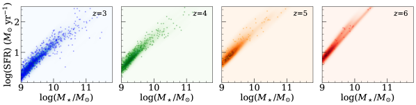
Figure 1: Total SFR as a function of the stellar mass for the sample galaxies. From left to right: $z=3$, $z=4$, $z=5$, and $z=6$.

2.2.1 TNG50 high-$z$ galaxies

The TNG50 simulation has already been shown to accurately reproduce the morphologies of galaxies at $z<3$ (Tacchella et al., 2019; Huertas-Company et al., 2019; Varma et al., 2022). In this work, we consider four TNG50 snapshots that correspond to galaxies at redshift $z=(3,4,5,6)$, selecting all galaxies with total stellar mass $M_{\star}>10^{9}$ $M_{\odot}$ at a given redshift. The parent sample is composed of 1334 galaxies. We limit our analysis to galaxies with a total half-mass radius larger than 1 arcsec, with $R_{\rm total}\sim 10R_{\rm half,\star}$, which translates to galaxies with a total diameter larger than $\sim 64$ pixels when simulated at the angular resolution of NIRCam in the F200W filter (see Sect. 3.1). With this selection, we exclude from our sample 8% of galaxies at $z=3$, 5% of galaxies at $z=4$, 1% of galaxies at $z=5$, and none of the galaxies at $z=6$. We checked that no bias is introduced by means of our selection in the parameter space of the final sample (i.e., the intrinsic mass-size plane is preserved at every redshift). In Vega-Ferrero et al. (in prep.), this criterion enables us to produce cutouts of a fixed size of $64\times 64$ pixels for all the galaxies, which will be ingested into a neural network for deriving galaxy morphologies.

With this selection, the final sample is composed of 1238 galaxies (see Table 1). To increase the sample statistics, each galaxy is observed in 20 different configurations, which correspond to 20 random orientations. In particular, we look at each galaxy under five inclinations $i=(0,45,90,135,180)$ degrees and four azimuths $a=(0,90,180,270)$ degrees. Thus, the final sample is composed of $24760$ galaxy projections. We detail in Table 1 their stellar mass median values and in Fig. 1 we show their total star-formation rate (SFR) distributions as a function of mass at different redshifts, showing that the vast majority of the sample is composed of star-forming galaxies.

3 Synthetic images

In this section, we describe the main steps to produce synthetic images tailored for JWST observations starting from cosmological simulations (Fig. 2). We first detail the methodology for post-processing galaxies in cosmological simulations to get noiseless images for NIRCam and MIRI in Sect. 3.1. We focus on CEERS observational strategy and describe how to create NIRCam-like raw data in Sect. 3.2. Finally, we briefly outline the main steps for reducing JWST imaging observations in Sect. 3.3.

3.1 NIRCam and MIRI noiseless images

In order to produce noiseless synthetic images of TNG50 high-$z$ galaxies, we modeled both the light distribution produced by stellar populations and star-forming regions and the effects of dust on radiation using the most recent version of SKIRT Monte-Carlo radiative transfer code (v9.0; Camps & Baes, 2015; Verstocken et al., 2017; Camps & Baes, 2020).

For each galaxy and each snapshot described in Sect. 2.2.1, we extract the corresponding sets of subhalo star particles and gas cells, while stellar wind particles are ignored. Each image has a side equal to twice the total half-mass radius of the corresponding galaxy, but greater than 2 arcsec (see Sect. 2.2.1). The number of pixels is chosen so that the resulting pixel scale matches that of JWST instruments. In particular, the spatial resolution is $0.11$ arcsec px^-1 for MIRI and $0.031$ ($0.063$) arcsec px^-1 for NIRCam short (long) channel.

In the following Sections, we describe the different steps that are required for the radiative transfer calculations. As a note of caution, several assumptions are necessary to post-process numerical simulations. We followed standard prescriptions from the literature (Rodriguez-Gomez et al., 2019; Camps & Baes, 2020; Shen et al., 2020; Kapoor et al., 2021), but different approaches could be explored (see e.g., Popping et al., 2022).

3.1.1 Stellar source

The primary source of emission is characterized by assigning each stellar particle a spectral energy distribution (SED) depending on its age in the simulation. On one side, old star particles ($t>10$ Myr) are modeled with a SED from the Bruzual & Charlot (2003) high-resolution template library and a Chabrier (2003) initial mass function. In our setup, SKIRT spatially distributes the photons from these sources using the smoothing length enclosing $32\pm 1$ nearest stellar particles for all stellar particles within the galaxy. On the other side, young stellar particles ($t<10$ Myr) are treated as unresolved regions of the interstellar medium (ISM) and are modeled with a SED from the MAPPINGS III library (Groves et al., 2008), which describes emission from both H II regions and the photo-dissociation region surrounding the star-forming core as well as absorption by gas and dust in the birth clouds of young stars. The MAPPINGS III models are parametrized by five parameters: (i) the metallicity of the star particle, (ii) the star formation rate (SFR), (iii) the compactness $C_{0}$ of the HII region, (iv) the pressure $P_{0}$ of the ISM, and (v) the covering fraction of the photo-dissociation region $f_{\rm PDR}$. In this work, we assume the metallicity to be the same as the birth environment of the young star particle (Vogelsberger et al., 2020), we assume that the SFR remains constant during the 10 Myr lifetime of the HII region (Rodriguez-Gomez et al., 2019), and we used typical values of $\log_{10}\sl{C_{0}}=5$, $\log[(P_{0}/k_{B})/{\rm cm}^{-3}{\rm K}]=5$, and $f_{\rm PDR}=0.2$ (Groves et al., 2008; Jonsson et al., 2010).

3.1.2 Dust modeling

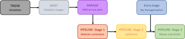
Figure 2: Workflow of the proposed forward modeling, from cosmological simulations to reduced NIRCam-like images, which mimic CEERS observations.

TNG50 does not include dust physics, hence we model the distribution of dust in the ISM using the properties (position, density, and metallicity) of the Voronoi gas cells. We select cold and star-forming gas cells ($T<8000$ K and SFR$>0$) and derive their metal and mass distribution (Kapoor et al., 2021). Following Shen et al. (2020), we assume that the metals in the ISM trace the dust component and convert the metal mass into the dust mass with a dust-to-metal ratio, which depends on redshift as $f_{\rm dust}=0.9\times(z/2)^{-1.92}$ (Vogelsberger et al., 2020). This empirical trend has been calibrated based on the observed UV luminosity functions of IllustrisTNG galaxies at redshift $z=2-10$. Thus, we set the dust density to be $\rho_{\rm dust}=f_{\rm dust}Z\rho_{\rm gas}$ for cold and star-forming gas cells and zero for all the other gas cells. The dust composition is modeled with the dust mix of Zubko et al. (2004), which includes graphite grains, silicate grains, and polycyclic aromatic hydrocarbons (Camps et al., 2016; Rodriguez-Gomez et al., 2019). This choice of multigrain models implies a correction in the dust density, which was decreased by 25% as described in Shen et al. (2020). Each type of dust has been discretized in 10 bins of grain sizes. The properties of the dust mix (sizes and abundances) are chosen so as to reproduce the dust properties of the Milky Way. Furthermore, for a more realistic description of UV to IR luminosities, we allow dust grains to be stochastically heated and decoupled from local thermal equilibrium, and we also include dust self-absorption and re-emission. The dust emission and self-absorption are repeated iteratively until the total luminosity absorbed by dust converges at a $<10\%$ level.

The dust density distribution is then discretized using an octree grid with a minimum refinement level of 3 and a maximum refinement level of 12 (Kapoor et al., 2021). We set a maximum cell dust fraction value of $10^{-6}$. It is worth noticing that within each grid cell, every physical quantity (e.g., the dust density, the radiation field, etc.) is assumed to be uniform.

3.1.3 Image signal-to-noise ratio

The quality of the final synthetic images is directly correlated to the number of photon packets employed in the radiative transfer simulation. SKIRT employs a wavelength grid for launching at each position $N_{\rm p}$ photon packets. The photons are collected by the detector after propagating through the resolved ISM and randomly interacting with the dust cells. On the one side, the more photons are employed in the simulation the higher the signal-to-noise ratio (SNR) of the final image. On the other side, $N_{\rm p}$ also drives the simulation run time. We tweak the number of required photon packets by looking at the relative error statistic described in Camps & Baes (2020). A good compromise between sufficient SNR and an acceptable simulation run time was found setting $N_{\rm p}=10^{8}$ photon packets per galaxy.

3.1.4 Synthetic data products

The post-processing of TNG50 galaxies allows us to create a set of synthetic observables comprised of noiseless images in multiple bands at different spatial resolutions, including spatially integrated fluxes of the total galaxy and each source component (i.e., primary and secondary emissions). In detail, we take advantage of SKIRT flexibility and observe each galaxy from 20 configurations. It is worth noticing that each additional configuration increases both the simulation run time and the memory consumption. At every observer position, we place a detector to mimic both NIRCam and MIRI observations. Each instrument provides both the spatially integrated flux and the images for each of NIRCam and MIRI filters (narrow, medium, and broadband) at the corresponding pixel scale (see Sect. 2.2.1). Thus, our TNG50 mock catalogue comprises noiseless images of 1238 galaxies at redshift $z=(3,4,5,6)$ seen from 20 different configurations in 27 NIRCam and 9 MIRI bands. Supplementary, a super-resolved version ($0.01$ arcsec px^-1) of each image is also available.

3.2 NIRCam raw images

We mimic NIRCam observations of TNG50 galaxies using the mirage (Multi Instrument Ramp Generator; Hilbert et al., 2019) simulator v2.2.1. This tool allows us to simulate imaging data that have the instrumental noise effects that will be present in in-flight data. The final raw data are created by adding astronomical sources to real dark current data from ground testing. The scenes could represent different levels of complexity, from point sources and Sérsic-profile galaxies, to more realistic morphologies from arbitrary fits images, like in our case.

Briefly, the simulation requires four stages: (1) it creates an input file with the observational settings exported from the Astronomer’s Proposal Tool (APT); (2) it creates a seed image, which corresponds to a noiseless image of the scene; (3) it prepares the dark current exposure; (4) it produces the final raw image (_uncal extension) considering the noise contributions both from the background and the detectors.

Our final scene is composed of a galaxy in the center and three reference stars, which are used to align the three dithered images in the final mosaic (Sect. 3.3.4) and build the observed point-spread function (PSF) for drizzled images (Appendix B).

3.3 Data reduction and calibration

Data simulated with mirage can be run through the JWST calibration pipeline v1.4.6 (CRDS v11.10.1), mimicking the data reduction strategy to be used for in-flight data. The calibration and reduction procedure takes place in three different stages, which are briefly detailed in the following sections (Fig. 2). The step-by-step description provided hereafter concerns the images obtained with detectors B1 and B5, which are used for the NIRCam filters F200W and F356W, respectively.

3.3.1 Stage 1: Detector corrections

The first stage of the JWST pipeline it is usually referred to as “ramps-to-slopes” processing, since it reads the non-destructive detector and it translates the integrations containing the accumulating counts (ramps) to uncalibrated images (slopes) in units of DN sec^-1. All the detector corrections are applied to all exposure types (e.g., imaging, spectroscopic, etc.).

In stage 1 multiple detector corrections are applied. The data quality initialization step populates the data quality mask, allowing the identification of dead pixels in the detector, highly non-linear pixels, and all sorts of quality flags. The saturation flagging step loops over all integrations within an exposure to flag all pixels where the signal is above the saturation limit. In the case of an integration with multiple groups, once one of them is flagged as saturated, also all subsequent groups for that pixel are flagged. For each integration in the input science data, the data are corrected group-by-group for interpixel capacitance. This step is usually skipped by default, but it was switched on in our reduction. The superbias subtraction step removes pixel by pixel the detector bias from every group in every integration of the science ramp data. The linearity correction step corrects science data values for detector non-linearity on a pixel-by-pixel, group-by-group, integration-by-integration basis. Based on a model, this step computes the number of traps that are expected to have captured or released a charge during an exposure. The released charge is proportional to the persistence signal, and this will be subtracted (group by group) from the science data. The persistence correction step subtracts group-by-group from the science data the number of traps that are expected to have captured or released a charge during an exposure. This step is of key importance for real observations, but it could have been skipped for our particular case, since mirage does not simulate this effect. The dark current subtraction step removes dark current from an exposure, group by group. The cosmic ray flagging step looks for outliers in the ramp of each pixel. It compares the signal in all the groups within an integration and it flags those with deviating more than $5\sigma$. The ramp fitting step produces a slope image for each integration (_rate extension).

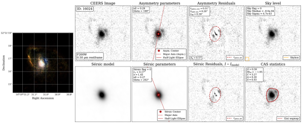
Figure 3: Example of morphological parameters derived with statmorph for galaxy ID 16024 ($z=3$, $M_{\star}\sim 10^{11}M_{\odot}$, $i=0$, $a=0$) in the F200W filter at 0.015 arcsec px^-1. On the left panel, we show the RGB synthetic image of the galaxy (0.01 arcsec px^-1), created using the F090W, F150W, and F200W noiseless data. Top row (from left to right): the CEERS image oriented with North up and East left, the asymmetry parameters (the galaxy center is shown as a red point, the half-light ellipse is shown as a solid red line, and the orientation of the major axis is shown as a dashed red line), the asymmetry residuals and size measurements (elliptical $r_{\rm petro}$ shown as a red dashed line), and sky statistics (median and rms in MJy sr^-1) with the sky region (orange box). Bottom row (from left to right): the noiseless Sérsic model, the Sérsic best fit parameters (the galaxy center is shown as a red point, the half-light ellipse derived from the Sérsic model is shown as a solid red line, and orientation of the major axis is shown as a dashed red line), Sérsic residuals, and non-parametric statistics (CAS, Gini, M₂₀) with the Gini segmentation map (red contour) derived as described in Rodriguez-Gomez et al. (2019).

3.3.2 Stage 2: Calibration

In stage 2, spectroscopic and imaging data are treated differently. For all JWST instruments, the imaging stage 2 is designed for calibrating individual slope images, providing data in units of MJy sr^-1. Firstly, the World Coordinate System (WCS) creation step allows to transform each position on the detector to a position in a world coordinate frame. The flat fielding step corrects for pixel-to-pixel sensitivity variations, dividing the science data set by a flat-field reference image. The photometric calibration step converts each image from units of countrate (ADU s^-1) to surface brightness (MJy sr^-1). The resample step corrects the flux-calibrated slope images from the effects of instrument distortions. As a result, individual fully calibrated (but unrectified) exposures are provided (_cal extension).

3.3.3 Extra Stage: Sky homogenization

Before stacking the individual frames obtained at a given sky position, we flattened and removed the background in all calibrated data images. This is done by fitting the image to a 3rd order two-dimensional polynomial, isolating the background pixels by masking all objects present in the field (in our case, only one galaxy and three reference stars). The final product of this step is a calibrated image with flat null background.

3.3.4 Stage 3: Mosaic

In stage 3, the calibrated data are combined according to the dither or mosaic pattern into a single rectified (distortion-corrected) image. A final step is applied to correct for astrometric alignment, background matching, and outlier rejection. As a result, a resampled and fully calibrated image is provided (_i2d extension), as well as a source catalog and a two-dimensional segmentation map. In this work, we combined the three exposures and created two datasets: the first one (v1.0) has images at nominal angular scale (0.063 and 0.031 arcsec px^-1 for short and long channels, respectively), while for the second one (v1.1) the images were drizzled to have a higher angular resolution (half-nominal), mimicking the strategy foreseen for CEERS observations (0.030 and 0.015 arcsec px^-1 for short and long channels, respectively).

4 Results and discussion

In this section we describe the main results of our analysis, focusing on the potential of CEERS in characterizing the morphology of galaxies at different redshifts ($3\leq z\leq 6$) and wavelengths (F200W, F356W). We discuss the measurements of galaxy sizes and morphological properties at half-nominal angular resolution, also investigating the effect that drizzling NIRCam images has on our measurements (see Appendix A).

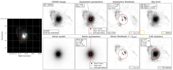
Figure 4: As in Fig. 3, but for the F356W filter at 0.030 arcsec px^-1. The RGB image is obtained using the F277W, F356W, and F444W filters.

4.1 Morphological measurements

We derive the parametric and non-parametric morphology of our sample galaxies using the standard configuration of statmorph, a Python package developed by Rodriguez-Gomez et al. (2019) and optimized to compute the optical morphologies of galaxies. All the details about the different sets of parameters derived with statmorph as well as the discussion about their definitions are fully explained by Rodriguez-Gomez et al. (2019).

Regarding the data quality, statmorph flags “bad measurements” either if there is a problem with the basic measurements (e.g., artifacts in the image or bad sky subtraction) or if there is a problem during the Sérsic fit, which could happen for galaxies with very irregular morphologies. Furthermore, we visually flag galaxies that are poorly detected or which have highly irregular segmentation maps. In the following, we will consider only galaxies with no flags, taking into account their redshift, filter, and angular resolution.

We recall that the primary objective of this work is to provide mock-observed morphological parameters, of simulated galaxies, for an easier comparison with the first JWST observations. We focus on different size estimators (e.g., the Petrosian radius $r_{\rm petro}$, the half-light radius from aperture photometry $r_{\rm half,phot}$, and the effective radius from the Sérsic fit $r_{\rm e}$), but we also derived the Gini coefficient, the M₂₀ statistic, the F(G,$M_{20}$) statistic, the galaxy concentration $C$, asymmetry $A$, smoothness $S$, and the Sérsic index $n$ (see Appendix A). For each of these measurements, each galaxy is considered a single-component system. As a complementary product of this work, we released the morphological catalog with all measured parameters.

In Figures 3 and 4 we provide an example of the measured parameters for the galaxy ID 16024 ($z=3$, $M_{\star}\sim 10^{11}~{}M_{\odot}$, $i=0$, $a=0$) in the F200W and F356W bands, respectively. Focusing on the RGB synthetic images, it can be appreciated that the galaxy shows a prominent tidal feature on the west side which is fading at longer wavelengths. This structure is detected both in the F200W and F356W bands, even though it is quite faint. Moreover, a prominent dust lane is situated on the east side of the galaxy, visible at short and long wavelengths both in the synthetic and calibrated images. The galaxy can be modeled with a Sérsic law with $n\sim 1.5$ ($n\sim 2$) and $r_{\rm e}\sim 0.15$ arcsec ($r_{\rm e}\sim 0.3$ arcsec) in the F200W (F356W) band. The intrinsic half-mass radius ($R_{\rm half,\star}$, see Sect. 4.2) is 0.79 kpc, which led to $r_{\rm e}$/$R_{\rm half,\star}$ = 1.75. From the residual maps, we can infer that the galaxy is probably hosting a central bulge embedded in an extended disk. Moreover, the galaxy is supported by rotation ($v_{\rm max}/\sigma\sim 2$), consistent with a late-type system of disk-like morphology, but already showing a prominent bulge.

Table 2: Median sizes of galaxies measured in the F200W band at different redshift.

. $z$ $R_{\rm half,\star}$ $r_{\rm e}$ $r_{\rm petro}$ $r_{\rm e}$/$R_{\rm half,\star}$ $r_{\rm petro}$/$r_{\rm e}$ (kpc) (kpc) (kpc) 3 $1.79^{+1.12}_{-0.72}$ $1.71^{+0.80}_{-0.50}$ $4.01^{+1.58}_{-0.98}$ 1.00^+0.53_-0.36 $2.32^{+1.43}_{-0.86}$ 4 $1.44^{+0.83}_{-0.68}$ $1.29^{+0.59}_{-0.39}$ $3.09^{+1.17}_{-0.77}$ 0.97^+0.50_-0.35 $2.27^{+1.48}_{-0.81}$ 5 $1.27^{+1.03}_{-0.63}$ $1.09^{+0.50}_{-0.36}$ $2.60^{+1.04}_{-0.75}$ 0.92^+0.57_-0.38 $2.15^{+1.81}_{-0.90}$ 6 $1.14^{+0.45}_{-0.90}$ $0.80^{+0.36}_{-0.38}$ $1.94^{+0.94}_{-0.58}$ 0.87^+0.99_-0.31 $2.08^{+4.08}_{-0.78}$

Note. — (1) Redshift. (2) Median value and 16th-84th percentile range of half-mass radius. (3) Median value of effective radius. (4) Median value of elliptical Petrosian radius. (5) Median value of the ratio $r_{\rm e}/R_{\rm half,\star}$. (6) Median value of the ratio $r_{\rm petro}/r_{\rm e}$.

Table 3: Median sizes of galaxies measured in the F356W band at different redshift. Columns as in Table 2.

. $z$ $R_{\rm half,\star}$ $r_{\rm e}$ $r_{\rm petro}$ $r_{\rm e}$/$R_{\rm half,\star}$ $r_{\rm petro}$/$r_{\rm e}$ (kpc) (kpc) (kpc) 3 $1.84^{+1.23}_{-0.76}$ $1.74^{+0.79}_{-0.52}$ $4.32^{+1.63}_{-1.02}$ 0.96^+0.51_-0.32 $2.36^{+1.36}_{-0.73}$ 4 $1.53^{+0.97}_{-0.69}$ $1.35^{+0.64}_{-0.41}$ $3.40^{+1.23}_{-0.77}$ 0.92^+0.44_-0.32 $2.26^{+1.37}_{-0.73}$ 5 $1.42^{+1.47}_{-0.74}$ $1.15^{+0.57}_{-0.35}$ $2.93^{+1.14}_{-0.73}$ 0.84^+0.46_-0.34 $2.15^{+1.56}_{-0.91}$ 6 $1.39^{+0.69}_{-0.86}$ $0.87^{+0.44}_{-0.33}$ $2.35^{+0.87}_{-0.62}$ 0.75^+0.56_-0.28 $1.93^{+3.85}_{-0.69}$

4.2 Size definitions

In this work, we discuss the evolution of sizes in high-$z$ massive galaxies in TNG50 and consider the following size measurements: the effective radius from the Sérsic fit ($r_{\rm e}$), the Petrosian radius measured on elliptical apertures ($r_{\rm petro}$), and the half-light radius derived from elliptical aperture photometry ($r_{\rm half,phot}$; see Appendix B). Finally, we used the three-dimensional stellar half-mass radius ($R_{\rm half,\star}$; Pillepich et al., 2019), which is measured as the three-dimensional radius containing half of the stellar mass of all constituent stars gravitationally bound to a galaxy, as a reference for the mass distribution of TNG50 galaxies.

The use of multiple size definitions in the literature (Sersic, 1968; Petrosian, 1976; Ferguson et al., 2004; Bouwens et al., 2004; Graham & Driver, 2005; Chamba et al., 2020) reflects the ambiguity in defining the total extent of a galaxy, which is assumed to contain its entire flux. For high-$z$ galaxies, the task of measuring their sizes is even more challenging, because (1) the irregular/chaotic morphology makes it difficult to define the galaxy center and perform aperture photometry; (2) the outskirt of the galaxy has very low surface-brightness features, usually not detected; (3) aperture photometry does not take into account the effect of the PSF (see Appendix B), while one-component (or multi-component) fitting is difficult because of the complex morphology of these galaxies; (4) the redshift of a given galaxy influences the surface density limits (i.e., cosmological dimming; Giavalisco et al., 1996; Ribeiro et al., 2016), so it is not straightforward to compare galaxies in a wide range of redshifts.

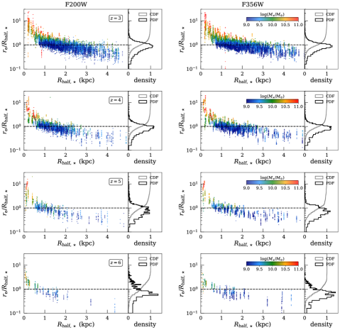
Figure 5: Comparison between $R_{\rm half,\star}$ and $r_{\rm e}$ for galaxies at different redshift (from top to bottom) in the F200W band (left panels) and F356W band (right panels). Main panels: Data points are color-coded according to the value of the galaxies’ total stellar mass. The black dashed line marks the 1:1 relation of the ratio $r_{\rm e}$/$R_{\rm half,\star}$. Side panels: probability density function (black solid line) and cumulative density function (gray solid line) of $r_{\rm e}$/$R_{\rm half,\star}$.

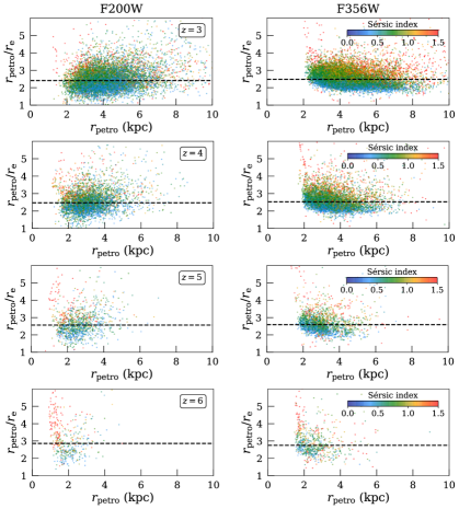
Figure 6: Comparison between $r_{\rm petro}$ and $r_{\rm e}$ for galaxies at different redshift (from top to bottom) in the F200W band (left panels) and F356W band (right panels). Data points are color-coded according to the value of the Sérsic index. The black dashed line marks the median value of the ratio $r_{\rm petro}$/$r_{\rm e}$.

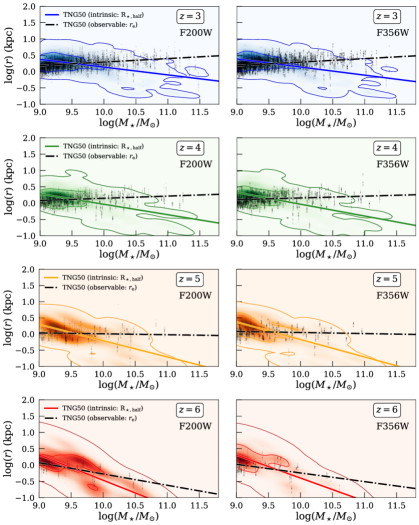
Figure 7: Mass-size relations from redshift $z=3$ (top panels) to $z=6$ (bottom panels). The left panels stand for sizes ($r_{\rm e}$ and R_⋆,half) measured in the F200W band and the right panels stand for those measured in the F356W band. The blue, green, orange, and red distributions and contours represent the values of R_⋆,half from TNG50, while the black points stand for the values of $r_{\rm e}$ measured on fully calibrated images. In each panel, the best-fit relation from Eq. 1 is shown with a colored solid line, while the one obtained from the mock observed TNG50 galaxies from Eq. 2 is shown as a dashed black line.

Table 4: Coefficients of the linear regression obtained for the mass-size relation at different redshifts in the F200W band.

. $z$ $a_{0}$ $b_{0}$ $a_{\rm obs}$ $b_{\rm obs}$ (kpc $M_{\odot}^{-1}$) (kpc) (kpc $M_{\odot}^{-1}$) (kpc) 3 $-0.24$ 2.48 0.09 $-0.65$ 4 $-0.33$ 3.27 0.05 $-0.39$ 5 $-0.55$ 5.25 $-0.05$ 0.44 6 $-0.78$ 7.29 $-0.27$ 2.44

Note. — (1) Redshift. (2) Slope of the linear trend from Eq. 1. (3) Intercept of the linear trend from Eq. 1. (4) Slope of the linear trend from Eq. 2. (5) Intercept of the linear trend from Eq. 2.

Table 5: As in Table 4, but for the F356W band.

. $z$ $a_{0}$ $b_{0}$ $a_{\rm obs}$ $b_{\rm obs}$ (kpc $M_{\odot}^{-1}$) (kpc) (kpc $M_{\odot}^{-1}$) (kpc) 3 $-0.26$ 2.72 0.11 $-0.80$ 4 $-0.35$ 3.48 0.06 $-0.47$ 5 $-0.55$ 5.27 $-0.03$ 0.34 6 $-0.71$ 6.71 $-0.27$ 2.42

4.3 Intrinsic and observable sizes

In this section we characterize the sizes of our galaxies by means of the Petrosian radius and the effective radius, describing the goodness/reliability of our measurements and the interplay between $r_{\rm petro}$ and $r_{\rm e}$. Throughout this section, we will consider sizes measured on images at half-nominal angular resolution. At each redshift, we report the median values of $r_{\rm e}$, $r_{\rm petro}$, and $R_{\rm half,\star}$ in Tables 2 and 3 for the F200W and F356W bands, respectively.

In Fig. 5, we present the evolution of $r_{\rm e}$ as a function of redshift and wavelength, comparing its distribution with the one of $R_{\rm half,\star}$. We find that the ratio $r_{\rm e}$/$R_{\rm half,\star}\sim 1$ at $z=3$ and $z=4$ (see also Figs. 9 and 10), and it starts to deviate at higher redshifts. The larger deviations are for small galaxies ($R_{\rm half,\star}<1$ kpc) and for large ones ($R_{\rm half,\star}>3$ kpc). In particular, the size of the most massive galaxies (e.g., $\log(M_{\star}/M_{\odot})>10.5$ at $z=3$) are overestimated, with deviations as large as $r_{\rm e}$/$R_{\rm half,\star}\sim 4-5$ (see also Wu et al., 2020). This behavior is seen both in the F200W and in the F356W band. In these galaxies, the light distribution is poorly fit by a single component, which overestimates the galaxy’s size and underestimates the central light concentration (see Appendix C). This could be interpreted as an indication of the build-up of the first (compact) bulges in disk galaxies, which happens at earlier cosmic time in more massive galaxies (Tacchella et al., 2015; Costantin et al., 2021, 2022). Besides these caveats, the trend presented in Fig. 5 shows that $r_{\rm e}$ is a good diagnostic for a galaxy’s mass-weighted size.

Regarding the effect that drizzling NIRCam images could have in retrieving their structural parameters, we find that a galaxy’s size increases by a factor up to 25% if measured on images at nominal angular resolution as compared to that measured on images at half-nominal angular resolution (see Appendix A). But, the size distribution at half-nominal angular resolution matches the intrinsic one retrieved from TNG50 (Fig. 5 and Figs. 9-10). Thus, we propose to discuss the structural evolution of our galaxies using the measured morphology on the drizzled images.

Furthermore, we quantify the difference between the sizes derived from $r_{\rm e}$ and $r_{\rm half,phot}$ (see Appendix B). In particular, we find that $r_{\rm e}$/$r_{\rm half,phot}<1$ mostly at all radii, presenting the largest deviations at small radii (up to 80-90%). Indeed, without considering any PSF correction, $r_{\rm half,phot}$ is not probing galaxy sizes smaller than $\sim 1$ kpc.

In Fig. 6 we illustrate the interplay between $r_{\rm petro}$ and $r_{\rm e}$ in describing the sizes of our galaxies. We quantify that, independent of redshift and photometric band, on average $r_{\rm petro}>2\times r_{\rm e}$ (see Tables 2 and 3). This trend, and the relation between $r_{\rm e}$ and $R_{\rm half,\star}$, raises a note of caution in limiting spectroscopic studies in the region covered by the effective radius, since this region is not even probing half of the mass distribution of the galaxy, or defining the total extension of the galaxy with a totally arbitrary factor (e.g., $2r_{\rm e}$). Indeed, the extension of the galaxy depends not only on the effective radius, but also on the shape of the surface-brightness profile (i.e., the light and mass distributions; Trujillo et al., 2020). As shown in Fig. 6, the ratio $r_{\rm petro}/r_{\rm e}$ depends on the value of the Sérsic index, since galaxies with $n<1$ show $r_{\rm petro}/r_{\rm e}<2.5$, while galaxies with $n>1$ show $r_{\rm petro}/r_{\rm e}>2.5$. For example, in the F200W band at $z=3$, the median values of these ratios are $2.31^{+0.57}_{-0.41}$ ($n<1$) and $2.67^{+0.61}_{-0.46}$ ($n>1$).

Finally, we compare the values of $r_{\rm petro}$ with the ones derived in Whitney et al. (2019) for a sample of 49,000 galaxies from the Cosmic Assembly Near-infrared Deep Extragalactic Survey (CANDELS; Grogin et al., 2011; Koekemoer et al., 2011). In particular, we see that the median size of our galaxies follows (within $1\sigma$) the redshift evolution expected for high-$z$ galaxies in the form of $r_{\rm petro}=12.62(1+z)^{-0.82}$, confirming the goodness of our predictions and already available observations targeting the ultraviolet rest-frame morphology (see Fig. 9 in Whitney et al., 2019). This could point to the fact that no (or mild) wavelength evolution of sizes is expected at these redshifts, at least comparing the restframe ultraviolet and optical morphology.

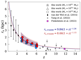
Figure 8: Evolution of size ($r_{\rm e}$) through redshift for galaxies in different mass bins. Stars stand for galaxies with $9\leq\log(M_{\star}/M_{\odot})\leq 9.25$, triangles stand for galaxies with $9.25<\log(M_{\star}/M_{\odot})\leq 9.6$, and dots stand for galaxies with $\log(M_{\star}/M_{\odot})>9.6$. Blue symbols correspond to median values in the F200W band, while red symbols represent the median value in the F356W band. The colored shaded regions mark the 16-84th percentile ranges. Black diamonds correspond to median sizes of late-type galaxies at $z<3$ with $\log(M_{\star}/M_{\odot})\sim 9.75$ (van der Wel et al., 2014). Gray squares stand for sizes measured in individual galaxies (NIRCam F356W band) at $z>7$ (Yang et al., 2022), while the purple cross corresponds to the Maisie’s Galaxy ($z=11.8$) identified in Finkelstein et al. (2022).

4.4 Expected size evolution of high-$z$ galaxies

Given that the effective radius measured on images at half-nominal angular resolution is a good proxy for the size of our galaxies as it reproduces the distribution of the half-mass radius, we provide in this section some ready-to-use diagnostics to discuss the structural evolution of high-$z$ galaxies observed with JWST. However, it is worth taking into account that there are (small) systematic deviations for the very large (and less massive) galaxies and for very compact (and most massive) galaxies.

In Fig. 7, we describe the redshift evolution of the mass-size relation of high-$z$ galaxies. We use the total stellar mass of the galaxy derived from TNG50 and the measured effective radius as a proxy for the galaxies’ size. We show the trend of the half-mass radius (density maps and contours of different colors) and the trend of the observable sizes, as measured by the effective radius (black symbols). We derived the coefficients of the best-fit (Tables 4 and 5) retrieved from parametrizing as a linear regression the intrinsic mass-size relation

$$\log(R_{\rm half,\star})=a_{0}\log(M_{\star})+b_{0}\,,$$ (1)

and the observable mass-size relation of the simulated galaxies

$$\log(r_{\rm e})=a_{\rm obs}\log(M_{\star})+b_{\rm obs}\,.$$ (2)

The first result is that, at all redshifts, there is almost no difference in the coefficients describing the linear parametrization of the mass-size relation derived at 2 $\mu$m and at 3.56 $\mu$m. This is true both for the intrinsic and observable parametrization, but with a discrepancy between the two. Indeed, the intrinsic mass-size relation shows a negative slope at all considered redshifts (see also Genel et al., 2018; Pillepich et al., 2019), while the size-mass trend based on observable $r_{\rm e}$ shows a transition from negative to positive slopes between $z=5$ and $z=4$. At each redshift, $r_{\rm e}$ is probing the trend of $R_{\rm half,\star}$ up to $\sim 5\times 10^{10}$ solar masses. For the more massive galaxies (i.e., the smaller ones in TNG50), $r_{\rm e}$ is overestimating their size (see also Fig. 5).

The negative slope of the intrinsic luminosity-size relation, apparently counter-intuitive, has also been presented in Marshall et al. (2022) for the BLUETIDES simulation (Feng et al., 2016) and in Roper et al. (2022) for the FLARES simulation (Lovell et al., 2021). At $z\gg 3$, according to multiple theoretical and observational predictions (e.g., Dekel & Burkert, 2014; Zolotov et al., 2015; Tacchella et al., 2015, 2016; Costantin et al., 2021), extreme events of gas compaction in massive galaxies could be responsible for building very massive and small galaxies. However, this intrinsic trend is in conflict with observations at these redshifts (e.g., Grazian et al., 2012; Shibuya et al., 2015; Bouwens et al., 2022, but see also Mosleh et al. (2020)). This mismatch could be due to several causes. First, the complex morphology of massive high-$z$ galaxies makes it difficult to reproduce the mass distribution with a single-component model. Second, some of the massive and compact bulges can be obscured by dust (e.g., Figs. 3 and 4). For instance, Roper et al. (2022) reported that galaxies at $z>5$ can even appear $\sim$50 times larger when including dust attenuation. Finally, it has to be considered that the effective radius is tracing the two-dimensional projection of the galaxy light and not its three-dimensional extension. While we find very mild evolution with wavelength (but targeting the UV/optical rest-frame spectral range), future JWST observations (e.g., MIRI/JWST), and analyses similar to the one proposed in this work, but targeting the reddest portion of the electromagnetic spectrum (e.g., Popping et al., 2022), could help in solving this apparent tension between predictions from cosmological simulations and observed sizes of high-$z$ galaxies.

We conclude our discussion by summarizing the size evolution with respect to mass, redshift, and wavelength in Fig. 8. Regarding the wavelength trend, at each redshift and mass, sizes measured in the F200W band are consistent (within $1\sigma$) with those measured in the F356W band. At $z=3$ and $z=4$, this could be explained by the fact that both bands are probing the optical restframe morphology. At higher redshift, this could be the consequence of the low number of galaxies and the fact that galaxies could present (similar) young stellar populations, which dominate the light in both bands. Regarding the mass trend, at redshift $z=3$ and $z=4$, more massive galaxies are larger than lower-mass ones (see also Fig. 7). At $z=5$ galaxies have similar sizes at all masses, while at $z=6$ the low-number statistics from the small TNG50 volume makes it difficult to provide any concluding result. But, for the most massive galaxies, we see a smooth transition from compact systems at higher redshift to more extended ones at lower redshift. This trend in the observable size-mass relation of the simulated galaxies, and the mismatch between the mass and light distribution, could be the consequence that these galaxies have complex morphology, not well described with just one component. They could present a central bulge, where most of the mass resides, and extended disky structures, biasing the light-weighted galaxy’s size to larger values than the mass-weighted one. Additionally, the central region of these massive galaxies could be obscured by dust (Wu et al., 2020).

Based on this interpretation, we speculate that from $z=5$ to $z=3$ there could be a turning point in galaxy evolution where the physical processes responsible to assemble the first compact systems, which are supposed to evolve into local elliptical or central bulges, are sub-dominant with respect to the physics regulating the disk growth (see e.g., Costantin et al., 2020, 2022). Finally, at all masses, galaxies at higher redshift are smaller (more concentrated) than those at lower redshift. The size evolution of galaxies can be parametrized as $r_{\rm e}=9.84(1+z)^{-1.26}$ in the F200W band and $r_{\rm e}=8.66(1+z)^{-1.15}$ in the F356W band. A similar trend is also confirmed by the evolution of the Petrosian radius, with $r_{\rm petro}=21.48(1+z)^{-1.21}$ in the F200W band and $r_{\rm petro}=18.30(1+z)^{-1.04}$ in the F356W band. The extrapolation of these trends towards lower redshifts is consistent with the observational measurements for massive late-type galaxies (van der Wel et al., 2014). Furthermore, we compared the first measurements of galaxies’ sizes in the primordial Universe, from $z\gtrsim 7$ (Yang et al., 2022) up to $z\sim 12$ (Finkelstein et al., 2022), with our estimated trends, finding overall very good agreement.

5 Summary and Conclusions

In this work, we created mock observations tailored for the forthcoming JWST observations of high-$z$ galaxies using a state-of-the-art cosmological simulation (i.e., TNG50). The main goal is to provide predictions for observable morphological parameters (i.e., by forward modeling stellar light), focusing on the galaxy’s size, to be compared right away with the first JWST datasets.

We generated $\sim 25,000$ synthetic images of $M_{\star}\geq 10^{9}$ $M_{\odot}$ galaxies from the TNG50 cosmological simulation at $z=3$, $z=4$, $z=5$, and $z=6$. The noiseless images were generated with the radiative transfer code SKIRT v9.0, including the effects of dust attenuation and scattering. The images are available in all the filters of the NIRCam and MIRI instruments of the JWST, at the corresponding angular resolution, i.e., 0.031 (0.063) arcsec px^-1 for NIRCam short (long) channel and 0.11 arcsec px^-1 for MIRI. A super-resolved version (0.01 arcsec px^-1) is also available.

As a second step, we simulated mock NIRCam observations following the observational strategy (e.g., noise, dithering pattern, etc.) of CEERS. Indeed, we processed the synthetic images with mirage and then calibrated them using the official JWST reduction pipeline, obtaining a set of mock observations in the F200W and F356W bands. The fully-calibrated images are available both at nominal angular resolution (0.031 arcsec px^-1 for F200W and 0.063 arcsec px^-1 for F356W), and at half-nominal angular resolution (0.015 arcsec px^-1 for F200W and 0.030 arcsec px^-1 for F356W), since we also drizzled them mimicking the strategy foreseen for CEERS (and many other wide-field surveys).

Finally, we measured with statmorph different size estimators (i.e., the Petrosian radius and the effective radius from the Sérsic fit), but we also derived the Gini coefficient, the M₂₀ statistic, the F(G,M₂₀) statistic, the galaxy concentration, asymmetry, smoothness, and the Sérsic index, which we released as a catalog associated with this work.

The expectations of the size evolution of massive galaxies at $3\leq z\leq 6$ from the TNG50 simulation of the IllustrisTNG suite can be summarized in the following points:

• We found that the (Sérsic) effective radius is a good proxy for the (three-dimensional) half-mass radius derived from TNG50 at all redshifts.

• On average, the Petrosian radius is found to be $r_{\rm petro}>2\times r_{\rm e}$.

• The sizes of high-$z$ galaxies are similar in the F200W and F356W bands. While for galaxies at $z=3$ and $z=4$ we are probing rest-frame optical morphology, for galaxies at $z=5$ and $z=6$ this could be explained by the fact that they present very young stellar populations.

• At all masses, higher-$z$ galaxies are smaller (more compact) than lower-$z$ ones.

• There is a mismatch in the mass and light distribution for the more massive galaxies, more evident at lower redshifts, since $r_{\rm e}>R_{\rm half,\star}$. Massive galaxies are more compact in mass than in observable stellar light, suggesting that their light distribution is not well-modeled with a single component and that they could be (heavily) obscured by dust. This points to the fact that there could be a morphological transition at $z=4-5$, which is responsible to build up the first generation of spheroids at $z\gg 3$, which could evolve in bulge+disk systems at lower redshift.

This work, and the companion work described in Vega-Ferrero et al. (in prep.) based on forward modeling of simulation data and their analysis using both classical and neural network techniques, will be extremely valuable in making a fair comparison between observations and predictions from cosmological simulations, as well as interpreting the formation and evolution of galaxies in the mostly unexplored high-$z$ regime. All data produced in this paper and related to the synthetic images of TNG50 galaxies for JWST-like NIRCam and MIRI observations is publicly available at https://www.tng-project.org/costantin22.

Appendix A Angular resolution effects

In this Appendix we quantified if/how different diagnostics are sensitive to the different angular resolutions of the observations. Unfortunately, to date this task was not carried out for high-$z$ galaxies, since the restframe optical morphology was inaccessible (at sufficient spatial resolution) with current facilities.

We focused on $z=3$ galaxies and compared the morphological measurements in the F200W band with angular scale of 0.031 arcsec px^-1 (nominal) with those at 0.015 arcsec px^-1 (half-nominal) and also those in the F356W band at 0.063 arcsec px^-1 (nominal) with those at 0.030 arcsec px^-1 (half-nominal). At $z=3$ we are targeting the restframe optical morphology of our galaxies in both NIRCam bands (0.50 $\mu$m in the F200W and 0.89 $\mu$m in the F356W), thus assuring only mild variation of morphology across wavelength. It is worth noting that we are actually probing the effect of drizzling NIRCam images for increasing (doubling) their spatial sampling, the ordinary strategy that it is foreseen to be adopted by forthcoming JWST observations. This task is of extreme importance in order to characterize how the galaxy morphology changes across wavelength, where images could be at different angular resolutions (see Sect. 4.4).

In the following, we focused on the following parameters: sizes ($r_{\rm petro}$ and $r_{\rm e}$), Sérsic index, Gini, M₂₀, F(G, M₂₀), and $CAS$ statistics. For the rest of the analysis, when referring to sizes, we will use the values measured on elliptical apertures. In Figs. 9 and 10, we first compare the difference between each parameter measured from images at nominal and at half-nominal angular resolution in both filters, while in Table 6, we reported the median values of each parameter.

In general, we see that sizes do depend on the angular resolution of the images. Both the Petrosian and the effective radius vary $\sim 25\%$ when measured in the F200W and $\sim 15\%$ when measured in the F356W band. We found that the median size is systematically larger if measured on images at nominal resolution, even if the values are within the $1\sigma$ variation. In the top middle panel of Fig. 9 we see that, at 2 $\mu$m, the distribution of the half-mass radius almost overlaps with the one of the effective radius measured on images at half-nominal angular resolution. In the F200W band, the median value of $r_{\rm e}$/$R_{\rm half,\star}=1.22^{+0.65}_{-0.35}$ at nominal and $r_{\rm e}$/$R_{\rm half,\star}=1.00^{+0.53}_{-0.36}$ at half-nominal angular resolution. At 3.56 $\mu$m (Fig. 10), $r_{\rm e}$ measured on images at half-nominal angular resolution still describes the half-mass radius better than the one at nominal angular resolution, even though both light-weighted measurements are not probing the tail of small sizes of our galaxies. In the F356W band, the median value of $r_{\rm e}$/$R_{\rm half,\star}=1.10^{+0.62}_{-0.30}$ at nominal and $r_{\rm e}$/$R_{\rm half,\star}=0.96^{+0.51}_{0.32}$ at half-nominal angular resolution.

The Sérsic index of the galaxies, being coupled with the effective radius, show a similar trend. The Gini coefficient is almost insensitive to angular resolution effects ($1-5\%$ variation), while M₂₀ and F(G,M₂₀) do slightly depend on the angular sampling of the images ($\sim 5-10\%$ variation for M₂₀ and $\sim 10-25\%$ variation for F(G,M₂₀)). The values are compatible within $1\sigma$ variation. Following a similar approach to the one applied in this work, Bignone et al. (2020) explored the impact of measuring the optical morphology of $z=0.1$ galaxies in the EAGLE simulations (Schaye et al., 2015; Crain et al., 2015; McAlpine et al., 2016) at different angular resolution. They found that the Gini coefficient systematically reduces with decreasing spatial resolution, while M₂₀ was almost not affected (median shifts less than 0.8 percent).

Finally, the $CAS$ statistics seem to be not well-suited to characterize the morphology of high-$z$ galaxies in our sample. Among the three diagnostics, the galaxy concentration is the only one that provides sensible results, being almost independent of the drizzling effect.

Table 6: Morphological parameters measured in the F200W and F356W bands at different angular resolutions for galaxies at $z=3$.

. Diagnostic Median value Median value Variation Median value Median value Variation (F200W nominal) (F200W half-nominal) (%) (F356W nominal) (F356W half-nominal) (%) $r_{\rm petro}$ (kpc) $4.97^{+2.03}_{-1.26}$ $3.90^{+1.51}_{-0.92}$ 24 $5.37^{+1.97}_{-1.48}$ $4.30^{+1.59}_{-1.01}$ 17 $r_{\rm e}$ (kpc) $2.11^{+0.88}_{-0.57}$ $1.61^{+0.69}_{-0.43}$ 25 $2.06^{+0.89}_{-0.62}$ $1.72^{+0.76}_{-0.51}$ 16 Sérsic index $0.80^{+0.39}_{-0.25}$ $0.65^{+0.37}_{-0.24}$ 24 $0.89^{+0.37}_{-0.26}$ $0.73^{+0.36}_{-0.23}$ 20 Gini $0.45^{+0.04}_{-0.02}$ $0.44^{+0.04}_{-0.02}$ 1 $0.50^{+0.04}_{-0.04}$ $0.47^{+0.04}_{-0.04}$ 5 M₂₀ $-1.30^{+0.27}_{-0.28}$ $-1.19^{+0.24}_{-0.32}$ 9 $-1.63^{+0.16}_{-0.13}$ $-1.58^{+0.16}_{-0.12}$ 3 F(G, M₂₀) $-0.84^{+0.40}_{-0.29}$ $-0.98^{+0.40}_{-0.24}$ -11 $-0.39^{+0.28}_{-0.26}$ $-0.56^{+0.26}_{-0.25}$ -26 Concentration $2.56^{+0.31}_{-0.26}$ $2.41^{+0.32}_{-0.26}$ 6 $2.64^{+0.26}_{-0.21}$ $2.48^{+0.24}_{-0.17}$ 6 Asymmetry $-0.20^{+0.09}_{-0.08}$ $-0.05^{+0.07}_{-0.06}$ 151 $-0.01^{+0.08}_{-0.06}$ $0.02^{+0.07}_{-0.06}$ -100 Smoothness $-0.07^{+0.04}_{-0.06}$ $0.02^{+0.03}_{-0.02}$ -262 $0.02^{+0.03}_{-0.02}$ $0.01^{+0.02}_{-0.01}$ 100

Note. — Values could slightly differ from those in other tables, because of the quality criteria explained in Sect. 4.1. (1) Morphological parameter. (2) Median value and 16th-84th percentile range at nominal angular resolution (0.031 arcsec px^-1) in the F200W band. (3) Median value and 16th-84th percentile range at half-nominal angular resolution (0.015 arcsec px^-1) in the F200W band. (4) Percentage of the variation between parameters at different angular resolutions. (5) Median value and 16th-84th percentile range at nominal angular resolution (0.063 arcsec px^-1) in the F356W band. (6) Median value and 16th-84th percentile range at half-nominal angular resolution (0.030 arcsec px^-1) in the F356W band. (7) Percentage of the variation between parameters at different angular resolutions.

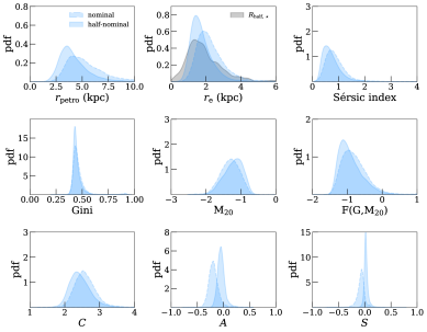
Figure 9: Distribution of morphological parameters measured in the F200W band. Top panel (from left to right): $r_{\rm petro}$, $r_{\rm e}$, and Sérsic index. Middle panel (from left to right): Gini, M₂₀, and F(G,M₂₀). Bottom panel (from left to right): concentration, asymmetry, and smoothness. The dashed lines mark the distributions at nominal angular resolution, while the solid lines define the distributions at half-nominal angular resolution. The distribution of $r_{\rm e}$ (top middle panel) can be compared with the one of $R_{\rm half,\star}$ (black curve).

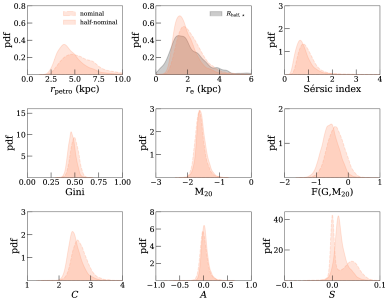
Figure 10: As in Fig. 9, but for the F356W band.

Appendix B PSF effects: $r_{\rm half,phot}$ and $r_{\rm e}$

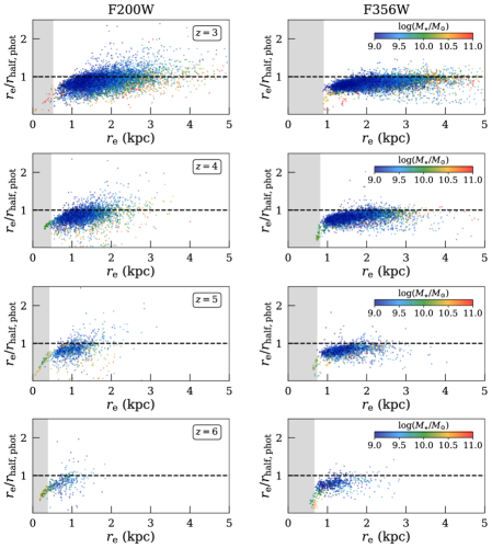
Figure 11: Comparison between $r_{\rm half,phot}$ and $r_{\rm e}$ for galaxies at different redshift (from top to bottom) in the F200W band (left panels) and F356W band (right panels). Data points are color-coded according to the value of the galaxies’ total stellar mass. The black dashed line marks the 1:1 relation of the ratio $r_{\rm e}$/$r_{\rm half,phot}$. The gray shaded regions mark the size of the full width at half maximum of the PSF at each redshift.

In this Appendix, we compared the role of the half-light radius and the effective radius in probing the size of our galaxies. Indeed, there is a meaningful difference in the two measurements, since $r_{\rm half,phot}$ does not take into account the effect of the PSF, while $r_{\rm e}$ does. Before running statmorph on the drizzled images (Sect. 4.1) and describing the galaxy light with a Sérsic model, we used the three stars in the NIRCam field-of-view and the photutils.psf package (Bradley et al., 2020) to built an observed PSF model (e.g., Cabello et al., 2022) at half-nominal angular resolution. Thus, we measured the galaxy size and compared the ratio between $r_{\rm half,phot}$ with $r_{\rm e}$ at different redshifts. In Fig. 11 we show how the trend between the two radii changes and how the $r_{\rm half,phot}$ and $r_{\rm e}$ distributions compare with the distribution of the half-mass radius. In particular, while the median value of $r_{\rm half,phot}$ is compatible with the median value of $R_{\rm half,\star}$, we can appreciate in Fig. 11 how $r_{\rm half,phot}$ is not able to describe the size of the smallest galaxies and the ratio $r_{\rm half,phot}/r_{\rm e}$ increasingly deviates from the 1:1 relation at smaller radii.

Appendix C 1D surface-brightness profiles: examples

In this Appendix, we provided some examples of the one-dimensional surface-brightness profiles of our galaxies ($z=3$, F356W). We measured the ellipse-averaged radial profiles of surface brightness both in the observed image and in the seeing-convolved model (Costantin et al., 2018a, b). We used the isophote.Ellipse.fit_image in Photutils from Python’s astropy package (Bradley et al., 2020).

In Fig. 12, we show two galaxies with $r_{\rm e}$/$R_{\rm half,\star}<1$ (ID 14287, ID 52297) and two galaxies with $r_{\rm e}$/$R_{\rm half,\star}>1$ (ID 3771, ID 16024). From this comparison, we see that the one-dimensional profiles of our Sérsic model seem reasonable, but the ratios $r_{\rm e}$/$R_{\rm half,\star}$ deviate from unity anyway. Thus, to fully constrain the complexity of these galaxies, we release both their images and the morphological catalog with every physical parameter. In this way, it is possible to properly derive the two-dimensional model and carefully study each individual object.

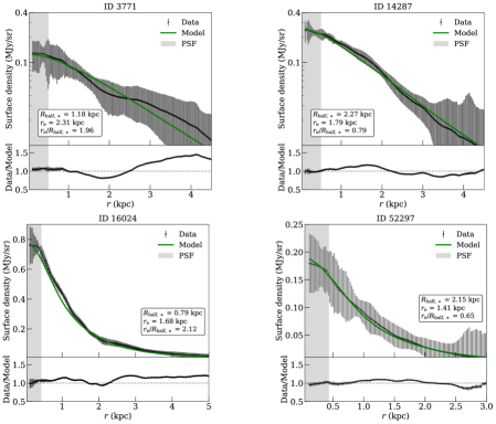
Figure 12: Ellipse-averaged radial profiles of surface brightness measured in the observed (black dots with grey error bars) and seeing-convolved modeled images (green solid line) and their corresponding difference.

References

- Bagley et al. (2022) Bagley, M. B., Finkelstein, S. L., Koekemoer, A. M., et al. 2022, arXiv e-prints, arXiv:2211.02495
- Bignone et al. (2020) Bignone, L. A., Pedrosa, S. E., Trayford, J. W., Tissera, P. B., & Pellizza, L. J. 2020, MNRAS, 491, 3624, doi: 10.1093/mnras/stz3014
- Bouwens et al. (2004) Bouwens, R. J., Illingworth, G. D., Blakeslee, J. P., Broadhurst, T. J., & Franx, M. 2004, ApJ, 611, L1, doi: 10.1086/423786
- Bouwens et al. (2022) Bouwens, R. J., Illingworth, G. D., van Dokkum, P. G., et al. 2022, ApJ, 927, 81, doi: 10.3847/1538-4357/ac4791
- Bradley et al. (2020) Bradley, L., Sipőcz, B., Robitaille, T., et al. 2020, astropy/photutils: 1.0.1, 1.0.1, Zenodo, Zenodo, doi: 10.5281/zenodo.4049061
- Bruzual & Charlot (2003) Bruzual, G., & Charlot, S. 2003, MNRAS, 344, 1000, doi: 10.1046/j.1365-8711.2003.06897.x
- Buitrago et al. (2008) Buitrago, F., Trujillo, I., Conselice, C. J., et al. 2008, ApJ, 687, L61, doi: 10.1086/592836
- Cabello et al. (2022) Cabello, C., Gallego, J., Cardiel, N., et al. 2022, A&A, 659, A116, doi: 10.1051/0004-6361/202141659
- Camps & Baes (2015) Camps, P., & Baes, M. 2015, Astronomy and Computing, 9, 20, doi: 10.1016/j.ascom.2014.10.004
- Camps & Baes (2020) —. 2020, Astronomy and Computing, 31, 100381, doi: 10.1016/j.ascom.2020.100381
- Camps et al. (2016) Camps, P., Trayford, J. W., Baes, M., et al. 2016, MNRAS, 462, 1057, doi: 10.1093/mnras/stw1735
- Cappellari (2016) Cappellari, M. 2016, ARA&A, 54, 597, doi: 10.1146/annurev-astro-082214-122432
- Chabrier (2003) Chabrier, G. 2003, PASP, 115, 763, doi: 10.1086/376392
- Chamba et al. (2020) Chamba, N., Trujillo, I., & Knapen, J. H. 2020, A&A, 633, L3, doi: 10.1051/0004-6361/201936821
- Costantin et al. (2018a) Costantin, L., Corsini, E. M., Méndez-Abreu, J., et al. 2018a, MNRAS, 481, 3623, doi: 10.1093/mnras/sty1754
- Costantin et al. (2018b) Costantin, L., Méndez-Abreu, J., Corsini, E. M., et al. 2018b, A&A, 609, A132, doi: 10.1051/0004-6361/201731823
- Costantin et al. (2020) —. 2020, ApJ, 889, L3, doi: 10.3847/2041-8213/ab6459
- Costantin et al. (2021) Costantin, L., Pérez-González, P. G., Méndez-Abreu, J., et al. 2021, ApJ, 913, 125, doi: 10.3847/1538-4357/abef72
- Costantin et al. (2022) —. 2022, ApJ, 929, 121, doi: 10.3847/1538-4357/ac5a57
- Crain et al. (2015) Crain, R. A., Schaye, J., Bower, R. G., et al. 2015, MNRAS, 450, 1937, doi: 10.1093/mnras/stv725
- Curtis-Lake et al. (2016) Curtis-Lake, E., McLure, R. J., Dunlop, J. S., et al. 2016, MNRAS, 457, 440, doi: 10.1093/mnras/stv3017
- Daddi et al. (2005) Daddi, E., Renzini, A., Pirzkal, N., et al. 2005, ApJ, 626, 680, doi: 10.1086/430104
- Dekel & Burkert (2014) Dekel, A., & Burkert, A. 2014, MNRAS, 438, 1870, doi: 10.1093/mnras/stt2331
- Driver et al. (1995) Driver, S. P., Windhorst, R. A., & Griffiths, R. E. 1995, ApJ, 453, 48, doi: 10.1086/176369
- Feng et al. (2016) Feng, Y., Di-Matteo, T., Croft, R. A., et al. 2016, MNRAS, 455, 2778, doi: 10.1093/mnras/stv2484
- Ferguson et al. (2004) Ferguson, H. C., Dickinson, M., Giavalisco, M., et al. 2004, ApJ, 600, L107, doi: 10.1086/378578
- Finkelstein et al. (2017) Finkelstein, S. L., Dickinson, M., Ferguson, H. C., et al. 2017, The Cosmic Evolution Early Release Science (CEERS) Survey, JWST Proposal ID 1345. Cycle 0 Early Release Science
- Finkelstein et al. (2022) Finkelstein, S. L., Bagley, M. B., Arrabal Haro, P., et al. 2022, arXiv e-prints, arXiv:2207.12474. https://arxiv.org/abs/2207.12474
- Genel et al. (2014) Genel, S., Vogelsberger, M., Springel, V., et al. 2014, MNRAS, 445, 175, doi: 10.1093/mnras/stu1654
- Genel et al. (2018) Genel, S., Nelson, D., Pillepich, A., et al. 2018, MNRAS, 474, 3976, doi: 10.1093/mnras/stx3078
- Giavalisco et al. (1996) Giavalisco, M., Steidel, C. C., & Macchetto, F. D. 1996, ApJ, 470, 189, doi: 10.1086/177859
- Graham & Driver (2005) Graham, A. W., & Driver, S. P. 2005, PASA, 22, 118, doi: 10.1071/AS05001
- Grazian et al. (2012) Grazian, A., Castellano, M., Fontana, A., et al. 2012, A&A, 547, A51, doi: 10.1051/0004-6361/201219669
- Grogin et al. (2011) Grogin, N. A., Kocevski, D. D., Faber, S. M., et al. 2011, ApJS, 197, 35, doi: 10.1088/0067-0049/197/2/35
- Groves et al. (2008) Groves, B., Dopita, M. A., Sutherland, R. S., et al. 2008, ApJS, 176, 438, doi: 10.1086/528711
- Hilbert et al. (2019) Hilbert, B., Sahlmann, J., Volk, K., et al. 2019, spacetelescope/mirage: First github release, v1.1.1, Zenodo, doi: 10.5281/zenodo.3519262
- Holwerda et al. (2020) Holwerda, B. W., Bridge, J. S., Steele, R. L., et al. 2020, AJ, 160, 154, doi: 10.3847/1538-3881/aba617
- Huertas-Company et al. (2016) Huertas-Company, M., Bernardi, M., Pérez-González, P. G., et al. 2016, MNRAS, 462, 4495, doi: 10.1093/mnras/stw1866
- Huertas-Company et al. (2019) Huertas-Company, M., Rodriguez-Gomez, V., Nelson, D., et al. 2019, MNRAS, 489, 1859, doi: 10.1093/mnras/stz2191
- Jonsson et al. (2010) Jonsson, P., Groves, B. A., & Cox, T. J. 2010, MNRAS, 403, 17, doi: 10.1111/j.1365-2966.2009.16087.x
- Kapoor et al. (2021) Kapoor, A. U., Camps, P., Baes, M., et al. 2021, MNRAS, 506, 5703, doi: 10.1093/mnras/stab2043
- Kartaltepe et al. (2022) Kartaltepe, J. S., Rose, C., Vanderhoof, B. N., et al. 2022, arXiv e-prints, arXiv:2210.14713
- Kocevski et al. (2022) Kocevski, D. D., Barro, G., McGrath, E. J., et al. 2022, arXiv e-prints, arXiv:2208.14480
- Koekemoer et al. (2011) Koekemoer, A. M., Faber, S. M., Ferguson, H. C., et al. 2011, ApJS, 197, 36, doi: 10.1088/0067-0049/197/2/36
- Lintott et al. (2011) Lintott, C., Schawinski, K., Bamford, S., et al. 2011, MNRAS, 410, 166, doi: 10.1111/j.1365-2966.2010.17432.x
- Lovell et al. (2021) Lovell, C. C., Vijayan, A. P., Thomas, P. A., et al. 2021, MNRAS, 500, 2127, doi: 10.1093/mnras/staa3360
- Marinacci et al. (2018) Marinacci, F., Vogelsberger, M., Pakmor, R., et al. 2018, MNRAS, 480, 5113, doi: 10.1093/mnras/sty2206
- Marshall et al. (2022) Marshall, M. A., Wilkins, S., Di Matteo, T., et al. 2022, MNRAS, 511, 5475, doi: 10.1093/mnras/stac380
- McAlpine et al. (2016) McAlpine, S., Helly, J. C., Schaller, M., et al. 2016, Astronomy and Computing, 15, 72, doi: 10.1016/j.ascom.2016.02.004
- Mortlock et al. (2013) Mortlock, A., Conselice, C. J., Hartley, W. G., et al. 2013, MNRAS, 433, 1185, doi: 10.1093/mnras/stt793
- Mosleh et al. (2020) Mosleh, M., Hosseinnejad, S., Hosseini-ShahiSavandi, S. Z., & Tacchella, S. 2020, ApJ, 905, 170, doi: 10.3847/1538-4357/abc7cc
- Mowla et al. (2019) Mowla, L. A., van Dokkum, P., Brammer, G. B., et al. 2019, ApJ, 880, 57, doi: 10.3847/1538-4357/ab290a
- Naiman et al. (2018) Naiman, J. P., Pillepich, A., Springel, V., et al. 2018, MNRAS, 477, 1206, doi: 10.1093/mnras/sty618
- Nelson et al. (2018) Nelson, D., Pillepich, A., Springel, V., et al. 2018, MNRAS, 475, 624, doi: 10.1093/mnras/stx3040
- Nelson et al. (2019) —. 2019, MNRAS, 490, 3234, doi: 10.1093/mnras/stz2306
- Oesch et al. (2010) Oesch, P. A., Bouwens, R. J., Carollo, C. M., et al. 2010, ApJ, 709, L21, doi: 10.1088/2041-8205/709/1/L21
- Papovich et al. (2005) Papovich, C., Dickinson, M., Giavalisco, M., Conselice, C. J., & Ferguson, H. C. 2005, ApJ, 631, 101, doi: 10.1086/429120
- Park et al. (2022) Park, C., Lee, J., Kim, J., et al. 2022, arXiv e-prints, arXiv:2202.11925
- Pérez-González et al. (2022) Pérez-González, P. G., Barro, G., Annunziatella, M., et al. 2022, arXiv e-prints, arXiv:2211.00045
- Petrosian (1976) Petrosian, V. 1976, ApJ, 210, L53, doi: 10.1086/182301
- Pillepich et al. (2018) Pillepich, A., Nelson, D., Hernquist, L., et al. 2018, MNRAS, 475, 648, doi: 10.1093/mnras/stx3112
- Pillepich et al. (2019) Pillepich, A., Nelson, D., Springel, V., et al. 2019, MNRAS, 490, 3196, doi: 10.1093/mnras/stz2338
- Planck Collaboration et al. (2016) Planck Collaboration, Ade, P. A. R., Aghanim, N., et al. 2016, A&A, 594, A13, doi: 10.1051/0004-6361/201525830
- Popping et al. (2022) Popping, G., Pillepich, A., Calistro Rivera, G., et al. 2022, MNRAS, 510, 3321, doi: 10.1093/mnras/stab3312
- Ravindranath et al. (2006) Ravindranath, S., Giavalisco, M., Ferguson, H. C., et al. 2006, ApJ, 652, 963, doi: 10.1086/507016
- Ribeiro et al. (2016) Ribeiro, B., Le Fèvre, O., Tasca, L. A. M., et al. 2016, A&A, 593, A22, doi: 10.1051/0004-6361/201628249
- Rodriguez-Gomez et al. (2019) Rodriguez-Gomez, V., Snyder, G. F., Lotz, J. M., et al. 2019, MNRAS, 483, 4140, doi: 10.1093/mnras/sty3345
- Roper et al. (2022) Roper, W. J., Lovell, C. C., Vijayan, A. P., et al. 2022, MNRAS, 514, 1921, doi: 10.1093/mnras/stac1368
- Schaye et al. (2015) Schaye, J., Crain, R. A., Bower, R. G., et al. 2015, MNRAS, 446, 521, doi: 10.1093/mnras/stu2058
- Sersic (1968) Sersic, J. L. 1968, Atlas de Galaxias Australes
- Shen et al. (2020) Shen, X., Vogelsberger, M., Nelson, D., et al. 2020, MNRAS, 495, 4747, doi: 10.1093/mnras/staa1423
- Shibuya et al. (2015) Shibuya, T., Ouchi, M., & Harikane, Y. 2015, ApJS, 219, 15, doi: 10.1088/0067-0049/219/2/15
- Sijacki et al. (2015) Sijacki, D., Vogelsberger, M., Genel, S., et al. 2015, MNRAS, 452, 575, doi: 10.1093/mnras/stv1340
- Snyder et al. (2015) Snyder, G. F., Torrey, P., Lotz, J. M., et al. 2015, MNRAS, 454, 1886, doi: 10.1093/mnras/stv2078
- Springel (2010) Springel, V. 2010, MNRAS, 401, 791, doi: 10.1111/j.1365-2966.2009.15715.x
- Springel et al. (2018) Springel, V., Pakmor, R., Pillepich, A., et al. 2018, MNRAS, 475, 676, doi: 10.1093/mnras/stx3304
- Suess et al. (2019) Suess, K. A., Kriek, M., Price, S. H., & Barro, G. 2019, ApJ, 877, 103, doi: 10.3847/1538-4357/ab1bda
- Tacchella et al. (2016) Tacchella, S., Dekel, A., Carollo, C. M., et al. 2016, MNRAS, 458, 242, doi: 10.1093/mnras/stw303
- Tacchella et al. (2015) Tacchella, S., Carollo, C. M., Renzini, A., et al. 2015, Science, 348, 314, doi: 10.1126/science.1261094
- Tacchella et al. (2019) Tacchella, S., Diemer, B., Hernquist, L., et al. 2019, MNRAS, 487, 5416, doi: 10.1093/mnras/stz1657
- Trayford et al. (2017) Trayford, J. W., Camps, P., Theuns, T., et al. 2017, MNRAS, 470, 771, doi: 10.1093/mnras/stx1051
- Trujillo et al. (2020) Trujillo, I., Chamba, N., & Knapen, J. H. 2020, MNRAS, 493, 87, doi: 10.1093/mnras/staa236
- Trujillo et al. (2007) Trujillo, I., Conselice, C. J., Bundy, K., et al. 2007, MNRAS, 382, 109, doi: 10.1111/j.1365-2966.2007.12388.x
- van der Wel et al. (2014) van der Wel, A., Franx, M., van Dokkum, P. G., et al. 2014, ApJ, 788, 28, doi: 10.1088/0004-637X/788/1/28
- Varma et al. (2022) Varma, S., Huertas-Company, M., Pillepich, A., et al. 2022, MNRAS, 509, 2654, doi: 10.1093/mnras/stab3149
- Verstocken et al. (2017) Verstocken, S., Van De Putte, D., Camps, P., & Baes, M. 2017, Astronomy and Computing, 20, 16, doi: 10.1016/j.ascom.2017.05.003
- Vogelsberger et al. (2014) Vogelsberger, M., Genel, S., Springel, V., et al. 2014, MNRAS, 444, 1518, doi: 10.1093/mnras/stu1536
- Vogelsberger et al. (2020) Vogelsberger, M., Nelson, D., Pillepich, A., et al. 2020, MNRAS, 492, 5167, doi: 10.1093/mnras/staa137
- Whitney et al. (2019) Whitney, A., Conselice, C. J., Bhatawdekar, R., & Duncan, K. 2019, ApJ, 887, 113, doi: 10.3847/1538-4357/ab53d4
- Wu et al. (2020) Wu, X., Davé, R., Tacchella, S., & Lotz, J. 2020, MNRAS, 494, 5636, doi: 10.1093/mnras/staa1044
- Yang et al. (2022) Yang, L., Morishita, T., Leethochawalit, N., et al. 2022, arXiv e-prints, arXiv:2207.13101. https://arxiv.org/abs/2207.13101
- Zolotov et al. (2015) Zolotov, A., Dekel, A., Mandelker, N., et al. 2015, MNRAS, 450, 2327, doi: 10.1093/mnras/stv740
- Zubko et al. (2004) Zubko, V., Dwek, E., & Arendt, R. G. 2004, ApJS, 152, 211, doi: 10.1086/382351