Simplifying a classical-quantum algorithm interpolation
with quantum singular value transformations

Abstract

The problem of Phase Estimation (or Amplitude Estimation) admits a quadratic quantum speedup. Wang, Higgott and Brierley [2019, Phys. Rev. Lett. 122 140504] have shown that there is a continuous trade-off between quantum speedup and circuit depth (by defining a family of algorithms known as $\alpha$-QPE). In this work, we show that the scaling of $\alpha$-QPE can be naturally and succinctly derived within the framework of Quantum Singular Value Transformation (QSVT). From the QSVT perspective, a greater number of coherent oracle calls translates into a better polynomial approximation to the sign function, which is the key routine for solving Phase Estimation. The better the approximation to the sign function, the fewer samples one needs to determine the sign accurately. With this idea, we simplify the proof of $\alpha$-QPE, while providing a new interpretation of the interpolation parameters, and show that QSVT is a promising framework for reasoning about classical-quantum interpolations.

I Introduction

With the developments in practical implementations of quantum computers, and with fault-tolerant computation still apparently beyond reach in the near future, much attention has been focused on classical-quantum (hybrid) algorithms: those that can leverage a limited amount of quantum coherence, while out-performing completely classical algorithms [1, 2, 3, 4]. That such hybrid algorithms exist for any given problem, and for any coherence time constraint, is not obvious. Explicitly showing the existence of a continuous trade-off between classical and quantum resources provides much insight on the role of the two types of resources in the algorithm, and how to off-load work from one to the other. Of course, the formulation of hybrid algorithms gives also the practical advantage of being able to adapt to the available quantum resources, such that, even when these are limited, a speed-up can be achieved.

One particular problem for which hybrid algorithms have been thoroughly studied is that of Phase Estimation. In this problem, we are given access to a unitary $U$ and an eigenstate $\ket{\psi}$ with eigenvalue $e^{i\phi}$, where the value of $\phi$ is unknown; the goal is to determine $\phi$. To understand the hybrid algorithm approaches to Phase Estimation, it is useful to first consider the Iterative Phase Estimation algorithm (also known as Kitaev’s Phase Estimation) [5, 6]. The method is obtained from the usual Quantum Fourier Transform-based Phase Estimation by invoking the deferred measurement principle, which produces the circuit of Figure 1. The circuit has the free parameters $M$ and $\theta$, which are updated at each iteration of the algorithm. Concretely, to obtain $\phi$ up to a precision of $2^{-m}$, one should set, at each step,

$$(M,\theta)_{1}=(2^{m-1},0)$$

$$(M,\theta)_{2}=(2^{m-2},-\pi\cdot 2^{-m}\cdot\phi_{m})$$

$$(M,\theta)_{3}=(2^{m-3},-\pi\cdot(2^{-m}\cdot\phi_{m}+2^{-m+1}\cdot\phi_{m-1}))$$

$$\hskip 78.06017pt\vdots$$

$$(M,\theta)_{m}=(1,-\pi\cdot(2^{-m}\cdot\phi_{m}+\cdots+2^{-2}\cdot\phi_{2}))$$

where, at step $j$, if $E$ is measured to be $1$, then $\phi_{m-j+1}=1$, and if $E=0$, $\phi_{m-j+1}=0$. By the end of the procedure, $\phi\approx\pi\sum_{j=1}^{m}2^{-j}\phi_{j}$, with precision $2^{-m}$.

Figure 1: Circuit for Iterative Phase Estimation. $U\ket{\psi}=e^{i\phi}\ket{\psi}$, $R_{Z}(x)=\outerproduct{0}{0}+e^{ix}\outerproduct{1}{1}$, $M\in\mathbb{N}$, $\theta\in\mathbb{R}$, and $E\in\{0,1\}$, with $M,\theta$ to be set as part of the algorithm.

This formulation opens the possibility for other choices of the update method for $M$ and $\theta$. Svore et al. [7] note that an informational perspective can be adopted, whereby one actually wishes to estimate a parameter of a distribution, and should seek to maximize the Fisher information of their measurements. By exploiting schedules that maximize information, they reduced the number of necessary samples in logarithmic factors, and approach that they call Fast Phase Estimation.

Nonetheless, both Fast Phase Estimation and the Iterative Phase Estimation have, up to polylogarithmic factors, the same requirements in terms of the total number of calls to $U$, denoted by $T$, and the required circuit depths, denoted by $D$: $T=\tilde{\mathcal{O}}(1/\epsilon),D=\mathcal{O}(1/\epsilon)$, where $\epsilon$ is the precision error attained in the estimation of $\phi$ . These requirements should be contrasted with those for the Hadamard Test, which corresponds essentially to a classical statistical sampling approach: the quantity of interest is encoded in the odds of a Bernoulli distribution, which can be optimally estimated to precision $\epsilon$ with $\mathcal{O}(1/\epsilon^{2})$ samples of the circuit [8], but with a single oracle call per run (thus with $D=\mathcal{O}(1)$).

Explorations of alternative schedules and associated classical algorithms brought Wiebe et al. to formulate Bayesian Phase Estimation [9], eventually leading to Wang et al.’s $\alpha$-Quantum Phase Estimation ($\alpha$-QPE) [10]. This approach established a continuous trade-off between depth and sampling complexity, and bridged the aforementioned Iterative Phase Estimation and statistical sampling. Giurgica-Tiron et al. [11] went on to rigorously show the convergence of these methods, and connected these hybridized Phase Estimation algorithms with other results on Quantum Fourier Transform-free Amplitude Estimation algorithms [12, 13].

Notably, $\alpha$-QPE describes the spectrum of hybrid Phase Estimation algorithms with a single scalar parameter — the titular $\alpha$ — such that the depth and sample complexity attained for a given choice of $\alpha$ and precision $\epsilon$ are $T=\mathcal{O}(1/{\epsilon^{1+\alpha}})$, and $D=\mathcal{O}(1/{\epsilon^{1-\alpha}})$, respectively. Note how the trade-off $TD$ remains a constant $\mathcal{O}(1/{\epsilon^{2}})$, and how this relationship is also verified both for statistical sampling and Iterative Phase Estimation.

Furthermore, Phase Estimation enjoys a close relationship with other notable algorithms; Brassard et al.’s algorithm for Amplitude Estimation [14] relies on it for a Grover-like operator. This places both Amplitude Estimation and Phase Estimation as central ingredients in many of quantum computing’s celebrated applications, such as Quantum Counting [15], Quantum Montecarlo [16], Quantum Linear Systems [17] or Ground State Preparation [18]. One also finds that using this relationship and the machinery of $\alpha$-QPE, a classical-quantum interpolation for Amplitude Estimation can likewise be found. As we will see, a similar relation also holds for the problem of Eigenvalue Estimation.

Recently, Gilyén et al. introduced Quantum Singular Value Transformation (QSVT) [19, 20]. As a generalization of the work of Quantum Signal Processing [21], it has proven to be an extremely powerful framework for describing quantum computation, having been shown by its authors to successfully describe quantum algorithms for search, Phase Estimation, and various quantum linear algebra results, among other applications.

In this work, we show that $\alpha$-QPE follows naturally from a Quantum Singular Value Transformation construction for Eigenvalue Estimation. This greatly simplifies the derivation of $\alpha$-QPE, if one is familiar with the main results of QSVT. At the same time, our method provides a different interpretation of the scalar parameter $\alpha$, namely relating it to the precision with which a step function is approximated by a constrained polynomial. Finally, this work may serve as a starting point for hybridizations of other relevant high-coherence algorithms under the QSVT description.

II Preliminaries

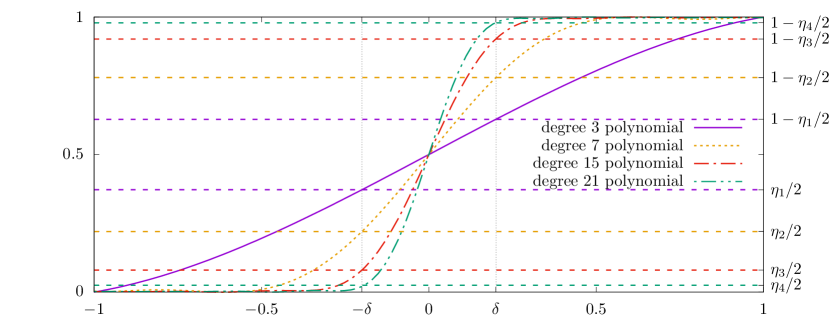
Figure 2: For a fixed $\delta$ (here, $\delta=0.2$), polynomials of increasing degree allow for a better approximation to the step function (equivalently, with a smaller $\eta$). While this decreases the necessary number of samples, the implementation of polynomials of higher degrees in the Quantum Singular Value Transformation framework requires longer coherent computation. A theorem of [22] ensures the existence of a suitable polynomial for a given choice of $\delta,\eta$ (cf. lemma 4); here we used the pyqsp [20, 23, 24] package to explicitly generate such polynomials.

II.1 Computational model

The analysis of $\alpha$-QPE is naturally set in a hybrid computing model [1, 4]. A hybrid classical-quantum algorithm is one that performs multiple runs of limited-depth quantum circuits, possibly interchangeably with some classical processing of the measurement outcomes.

The problems that we are concerned with here are defined in an oracular setting. That is, they are specified in terms of access to some given operators that encode the relevant information. Thus, our complexity measures are based on the number of oracle calls (or queries). The depth complexity of the algorithm, $D$, is the maximum depth among all the employed quantum circuits. The time complexity, $T$, is the total running time, that is, the sum of all the depths or, equivalently, the total number of queries.

Evidently, every $T$-time, $D$-depth algorithm can be converted into a $T$-time, $\mathcal{O}(T)$-depth algorithm [25]. But, in the context of limited-coherence computing, it becomes relevant to bound $D$ as much as possible. Moreover, in certain situations it may be beneficial to lower the depth complexity even if at the cost of increasing the total running time. This trade-off between $T$ and $D$ is achieved by $\alpha$-QPE.

Theorem 1 ($\alpha$-QPE, Proposition 1 of [10] and Theorem 2.3 of [11]).

For any $\alpha\in[0,1]$, there is a $T(\alpha)$-time, $D(\alpha)$-depth algorithm that solves PE, where

$$T(\alpha)=\mathcal{O}\left(\frac{1}{\epsilon^{1+\alpha}}\right)\;\text{and }\;D(\alpha)=\mathcal{O}\left(\frac{1}{\epsilon^{1-\alpha}}\right).$$ (1)

II.2 Problem reductions

As we have discussed, the problems of Phase Estimation and Amplitude Estimation are closely related. They also relate to the problem of Eigenvalue Estimation. Below, we precisely define each of these.

Phase estimation (PE). Let $U$ be a unitary operator and $\ket{\psi}$ a state such that $U\ket{\psi}=e^{i\phi}\ket{\psi}$ for some unknown $\phi\in[0,2\pi)$. Let $U_{\psi}$ be an operator that prepares $\ket{\psi}$: $U_{\psi}\ket{0^{m}}=\ket{\psi}$. Input: Access operators $U_{\psi}$, $U_{\psi}^{\operatorname*{\dagger}}$, controlled-$U$, and controlled-$U^{\operatorname*{\dagger}}$, and a precision parameter $\epsilon>0$. Output: An estimation of $\phi$ up to $\epsilon$, with bounded-error probability.

Amplitude estimation (AE). Let $A$ be a unitary operator such that $A\ket{0^{m}}=\sqrt{p}\ket{\text{good}}+\sqrt{1-p^{2}}\ket{\text{bad}}$ and let $O_{A}$ be an oracle that distinguishes $\ket{\text{good}}$ from $\ket{\text{bad}}$ (say, by applying a $-1$ phase to $\ket{\text{good}}$). Input: Access to operators $A$, $A^{\operatorname*{\dagger}}$, and $O_{A}$, and a precision parameter $\epsilon>0$. Output: An estimation of $|p|$ up to $\epsilon$, with bounded-error probability.

Before defining Eigenvalue Estimation, we need to introduce the concept of block-encoding, which permits representing non-unitary matrices in quantum circuits. We say that an $n$-qubit matrix $H$ is $(\gamma,m)$–block-encoded in an $(m+n)$ unitary matrix $U_{H}$ if

$$H=\gamma\left(\bra{0^{m}}\otimes I_{n}\right)U_{H}\left(\ket{0^{m}}\otimes I_{n}\right).$$ (2)

Eigenvalue estimation (EE). Let $H$ be a Hermitian operator and $\ket{\psi}$ a state such that $H\ket{\psi}=\mu\ket{\psi}$ for some unknown $\mu$. Let $U_{H}$ be a $(\gamma,m)$–block-encoding of $H$ and let $U_{\psi}$ prepare $\ket{\psi}$: $U_{\psi}\ket{0^{m}}=\ket{\psi}$. Input: Access to operators $U_{\psi}$, $U_{H}$, and $U_{H}^{\operatorname*{\dagger}}$, the factor $\gamma$, and a precision parameter $\epsilon>0$. Output: An estimation of $\mu$ up to $\epsilon$, with bounded-error probability.

Typically, these three computational problems are taken to be equivalent. This notion can be made rigorous. Given two problems $\mathrm{Pr}_{1}$ and $\mathrm{Pr}_{2}$, we write $\mathrm{Pr}_{1}\preceq\mathrm{Pr}_{2}$ if a $T$-time, $D$-depth algorithm to solve $\mathrm{Pr}_{2}$ can be converted into a $\mathcal{O}(T)$-time, $\mathcal{O}(D)$-depth algorithm to solve $\mathrm{Pr}_{1}$. In Appendix A, we show the following.

Lemma 2.

$\mathrm{PE}\preceq\mathrm{AE}\preceq\mathrm{EE}$.

Throughout the rest of the article, we will only be concerned with the EE problem. By Lemma 2, our results apply immediately also to PE and AE.

II.3 Quantum eigenvalue transformations

We approach EE with the filtering method developed by Lin and Tong [22], relying on the general theory for quantum singular value transformations [19]. Here we briefly review the main results that we need.

Let $H$ be a Hermitian matrix with a spectral decomposition $\{\mu_{i},\ket{\psi_{i}}\}_{i}$. For any function $F$, we define the eigenvalue transformation $F(H)$ as

$$H=\sum_{i}\mu_{i}\outerproduct{\psi_{i}}{\psi_{i}}\rightarrow F(H):=\sum_{i}F(\mu_{i})\outerproduct{\psi_{i}}{\psi_{i}}.$$ (3)

The idea of quantum eigenvalue transformations  is that, given a block encoding of $H$, we can perform a very broad class of polynomial transformations on $H$ in a time proportional to the degree of the polynomials.

Theorem 3 (Quantum eigenvalue transformations, Theorem 2 of [19]).

Let $U_{H}$ be a $(\gamma,m)$–block-encoding of a Hermitian matrix $H$ and let $P\in\mathbb{R}[x]$ be a $d$-degree polynomial with definite parity and $|P(x)|\leq 1$ for any $x\in[-1,1]$. Then, there is a $(1,m+1)$–block-encoding of $P(H/\gamma)$ using $d$ queries of $U_{H}$ and $U_{H}^{\operatorname*{\dagger}}$.

In particular, it is possible to approximate the sign function up to a desired accuracy [19, Lemma 14]. This is used by Lin and Tong [22] to block-encode an approximation of a projector onto the subspace of eigenstates with eigenvalues larger than some threshold $\mu_{0}$. See Figure 2 for an illustration of this construction.

Lemma 4 (Block-encoding approximation of step function, Lemma 5 of [22]).

Let $U_{H}$ be a $(\gamma,m)$-block-encoding of a Hermitian matrix $H$ and $\mu_{0}\in[0,\gamma]$. Then, there is a $(1,m+3)$–block-encoding of $P\left(\frac{H-\mu_{0}I}{\gamma+\mu_{0}};\delta,\eta\right)$, where $P$ satisfies

$$\forall x\in[-1,-\delta],0\leq P(x;\delta,\eta)\leq\eta/2$$ (4)

and $$\forall x\in[\delta,1],1-\eta/2\leq P(x;\delta,\eta)\leq 1,$$ (5)

using $\mathcal{O}\left(\frac{1}{\delta}\log(\frac{1}{\eta})\right)$ queries of $U_{H}$ and $U_{H}^{\operatorname*{\dagger}}$.

In their work, Lin and Tong [22] apply this construction to the problem of ground energy estimation with a binary search scheme. We adopt a similar strategy to the EE problem, re-deriving the scaling of $\alpha$-QPE.

III $\alpha$-QPE from quantum eigenvalue transformations

The classical-quantum interpolation is perhaps simpler to appreciate for the decision version of EE: given the same setting as EE and a parameter $\mu_{0}\in[-\gamma,\gamma]$, the task is to determine with bounded-error probability if $\mu$ is smaller than $\mu_{0}-\epsilon/2$ or greater than $\mu_{0}+\epsilon/2$, under the promise that one must be true. We focus on this problem for now and later we see how to turn this into a solution for the complete estimation task.

Using the construction from Lemma 4, we block-encode the step function approximation $P$, centered at $\mu_{0}$. We then measure the first $m+3$ qubits (i.e., the block-encoding register), assigning an outcome RIGHT to $\ket{0^{m+3}}$ and an outcome LEFT otherwise. Now, choose

$$\delta=\frac{\epsilon}{4\gamma}.$$ (6)

Then, if $\mu<\mu_{0}-\epsilon/2$, the probability of observing RIGHT is smaller than $(\eta/2)^{2}$. In contrast, if $\mu>\mu_{0}+\epsilon/2$, the probability of that outcome is greater than $(1-\eta/2)^{2}$. So, all that we have to do is to distinguish the bias of the Bernoulli distribution of LEFT/RIGHT outcomes with a precision smaller than

$$\frac{1}{2}\left((1-\eta/2)^{2}-(\eta/2)^{2}\right)=\frac{1-\eta}{2}.$$ (7)

By Chebychev’s inequality, we reach such an estimate with bounded-error probability by taking

$$\mathcal{O}\left(\frac{1}{(1-\eta)^{2}}\right)$$ (8)

trials.

We have the freedom to tune $\eta$ as desired. The lower the value of $\eta$, the fewer trials are necessary. On the other hand, a low $\eta$ requires a polynomial of a high degree, meaning more coherent applications of $U_{H}$ and $U_{H}^{\operatorname*{\dagger}}$.

For example, with a single application of $U_{H}$ we can only prepare a polynomial of degree one. In particular, the construction of Lemma 4 implements a block-encoding of $\frac{1}{2}\left(I+\frac{H-\mu_{0}I}{\gamma+\mu_{0}}\right)$. A straightforward calculation shows that, in this case, we need to estimate the bias of the LEFT/RIGHT Bernoulli distribution with precision at least $\epsilon/4\gamma$, requiring $\mathcal{O}(\gamma^{2}/\epsilon^{2})$ trials. This is but a classical statistical sampling approach.

Considering the other extreme case, say that we just want to take $\mathcal{O}(1)$ trials. From expression (8), we then need to set $\eta=1-\mathcal{O}(1)$, which leads to circuits of depth

$$\mathcal{O}\left(\frac{\gamma}{\epsilon}\log(\frac{1}{1-\mathcal{O}(1)})\right)=\mathcal{O}\left(\frac{\gamma}{\epsilon}\right).$$ (9)

This is precisely the scaling of the Phase Estimation algorithm.

We can reach a continuous interpolation between the classical and quantum regimes  by setting, for example,

$$\eta=1-\frac{1}{2}\left(\frac{\epsilon}{4\gamma}\right)^{\alpha}.$$ (10)

for $\alpha\in[0,1]$. From Lemma 4, the circuit depths are

$$D(\alpha) =\mathcal{O}\left(\frac{\gamma}{\epsilon}\log(\frac{1}{1-\left(\frac{\epsilon}{\gamma}\right)^{\alpha}})\right)$$

$$=\mathcal{O}\left(\left(\frac{\gamma}{\epsilon}\right)^{1-\alpha}\right).$$ (11)

Combining this with expression (8), we see that the total running time is

$$\mathcal{O}\left(D(\alpha)\left(\frac{\gamma}{\epsilon}\right)^{2\alpha}\right)=\mathcal{O}\left(\left(\frac{\gamma}{\epsilon}\right)^{1+\alpha}\right).$$ (12)

Finally, we may abandon the promise setting and convert the described procedure into a routine that decides if the eigenenergy $\mu$ is smaller or greater than some given threshold $\mu_{0}$, with tolerance for error if $|\mu-\mu_{0}|\leq\epsilon/2$. Then, with a standard binary search scheme we solve EE with just a $\mathrm{polylog}(\gamma/\epsilon)$ overhead to the decision version, but keeping the same essential $\alpha$-QPE scaling. We lay out the detailed steps in Algorithm 1. Applying the arguments above, we conclude the following.

Theorem 5.

Algorithm 1 solves EE up to precision $\epsilon$ with error probability smaller than $1/3$ using a total of

$$T(\alpha)=\mathcal{O}\left(\left(\frac{\gamma}{\epsilon}\right)^{1+\alpha}\log^{2}\left(\frac{\gamma}{\epsilon}\right)\right)$$ (13)

queries to $U_{H}$ and $U_{H}^{\operatorname*{\dagger}}$ and with depth

$$D(\alpha)=\mathcal{O}\left(\left(\frac{\gamma}{\epsilon}\right)^{1-\alpha}\right).$$ (14)

input : Access to operators $U_{\psi}$, $U_{H}$, and $U_{H}^{\operatorname*{\dagger}}$, the factor $\gamma$, and a precision parameter $\epsilon>0$, as defined in Section II.2, and an interpolating parameter $\alpha$.

output : Estimate of $\mu$ up to precision $\epsilon$ with error probability smaller than $1/3$.

1 def DecideEE($\mu_{0};\delta,\eta$):

2       Block-encode $P\left(\frac{H-\mu_{0}I}{\gamma+\mu_{0}};\delta,\eta\right)$ as in Lemma 4 and take $20\left(\frac{4\gamma}{\epsilon}\right)^{2\alpha}\lceil\log(\frac{4\gamma}{\epsilon})\rceil$ LEFT/RIGHT samples;

3       Estimate probability of RIGHT, $\overline{p}_{R}=(\text{number of {RIGHT}\ outcomes}/\text{number of trials})$;

4       if $\overline{p}_{R}>\frac{1-\eta+2\eta^{2}}{2}$ then

5             return RIGHT

6      else

7             return LEFT

8      

9$\delta\leftarrow\frac{\epsilon}{4\gamma}$, $\eta\leftarrow 1-\frac{1}{2}\left(\frac{\epsilon}{4\gamma}\right)^{\alpha}$;

10 $L\leftarrow-\gamma,R\leftarrow\gamma$;

11 while $R-L>\epsilon$ do

12       $\mu_{0}\leftarrow\lfloor(L+U)/2\rfloor$;

13       if outcome of DecideEE($\mu_{0};\delta,\eta$) is RIGHT then

14             $L\leftarrow\mu_{0}$;

15            

16      else

17             $R\leftarrow\mu_{0}$;

18            

19      

return $\mu_{0}$

Algorithm 1 Eigenvalue Estimation

IV Discussion

We have shown that the scaling of $\alpha$-QPE can be naturally derived from the framework of Quantum Singular Value Transformation (at least, up to polylogarithmic factors in the number of samples). QSVT approaches Phase Estimation by block-encoding an approximation to the sign function (which is here adapted into a step function). Our main contribution was to note that we can trade-off the quality of this approximation by longer statistical sampling. That is, we can compensate the use of lower degree polynomials (meaning lower circuit depths) by running the quantum circuits more times.

Our derivation provides a new interpretation of the parameter $\alpha$ on $\alpha$-QPE. Recalling that we approximate the step function up to error $\eta/2$ outside the interval $[-\delta,\delta]$, the approximation parameters $\eta,\delta$ and the interpolating parameter $\alpha$ are related as $\eta+\frac{1}{2}\delta^{\alpha}=1$. So, $\alpha$ translates how the two approximation parameters are related, parametrizing a family of approximations to the step function.

We believe that our proof is quite intuitive, given familiarity with QSVT theory, as $D(\alpha)$ follows immediately from the construction of the polynomial approximation to the step function. Indeed, the analysis reduces to checking how many samples do we have to take if we can only approximate the step function up to a certain degree. This reasoning circumvents the ad hoc approximations of Wang et al. [10], as well as the information theoretic considerations of Giurgica-Tiron et al. [11].

When converting the decision version of Eigenvalue Estimation into the full search problem we gained a $\mathcal{O}(\log^{2}\left(\frac{\gamma}{\epsilon}\right))$ factor that is not present in the original $\alpha$-QPE. Notably, this overhead appears only in the number of samples to collect, not in the circuit depth, for which our results match the state-of-the-art. Considering the current landscape of noisy, small-scale quantum computing, while any overhead in depth can be important, such a small overhead in number of samples is arguably not so significant. Regardless, it would still be interesting to find an optimal QSVT-based hybrid protocol. We conjecture that by further exploiting the structure of the polynomial approximation within the $[-\delta,\delta]$ interval one could remove the polylogarithmic overhead, but a rigorous proof is left as an open challenge.

Finally, our work shows that QSVT is not only a unifying framework for quantum algorithms, but also a useful tool to study hybrid computing. We suggest taking the perspective that more coherence time means better polynomial approximations to the target functions, reducing the need for repetitions. This line of reasoning may lead to the discovery of new classical-quantum interpolations.

Appendix A Proof of Lemma 2

A.1 $\mathrm{PE}\preceq\mathrm{AE}$

Let $(U_{\psi},U_{\psi}^{\operatorname*{\dagger}},\mathrm{controlled-}U,\mathrm{controlled-}U^{\operatorname*{\dagger}},\epsilon)$ be an instance of the PE problem, following the notation of Section II.2. Let $\ket{\psi}$ be a state of an $m$-qubit system. Now identify the operator $A$ with the following circuit.

$$\Qcircuit@C=1em@R=1em{&\qw{{}^{m}/}\gate{U_{\psi}}\gate{U}\qw\qw\\ \lstick{a\big{\{}}\qw\gate{H}\ctrl{-1}\gate{H}\qw}$$

This makes only one call to $U_{\psi}$ and $\mathrm{controlled-}U$. Similarly, $A^{\operatorname*{\dagger}}$ only makes one call to $U_{\psi}^{\operatorname*{\dagger}}$ and $\mathrm{controlled-}U^{\operatorname*{\dagger}}$. Identify $O_{A}$ with a $Z$ gate acting on the $a$ register.

Applying $A$ to $\ket{0^{m}}\ket{0}$ yields the state (up to a global phase factor)

$$A\ket{0^{m}}\ket{0}=\cos(\phi/2)\ket{\psi}\ket{0}-i\sin(\phi/2)\ket{\psi}\ket{1}.$$ (15)

So, we can solve AE with the instance $(A,A^{\operatorname*{\dagger}},O_{A},\epsilon)$ to get an estimate for $\phi$: if the output of AE is $\overline{p}$, then $2\arccos(\overline{p})$ is an $\epsilon$-close estimate to $\phi$. If the algorithm for AE takes time $T$ and depth $D$, then this algorithm for PE takes at most time $2T$ and depth $2D$.

A.2 $\mathrm{AE}\preceq\mathrm{EE}$

Let $(A,A^{\operatorname*{\dagger}},O_{A},\epsilon)$ be an instance of the AE problem, defined on $m$ qubits, and let

$$Q:=A\left(2\outerproduct{0^{m}}{0^{m}}-I\right)A^{\operatorname*{\dagger}}O_{A}.$$ (16)

Brassard et al. [14] show that we can write

$$A\ket{0^{m}}=\frac{1}{\sqrt{2}}\ket{\psi_{+}}+\frac{1}{\sqrt{2}}\ket{\psi_{-}}$$ (17)

where $\ket{\psi_{\pm}}$ are eigenvectors of $Q$ with eigenvalues $\exp(\pm 2i\arcsin{\sqrt{p}})$.

Identify $U_{\psi}$ with $A$, and $U_{H}$ with the following circuit.

$$\Qcircuit@C=1em@R=.5em{\lstick{a\big{\{}}&\qw\gate{H}\ctrl{1}\ctrlo{1}\gate{H}\\ \qw{{}^{m}/}\qw\gate{Q}\gate{Q^{\operatorname*{\dagger}}}\qw}\vspace{1pt}$$

Note that both $U_{H}$ and $U_{H}^{\operatorname*{\dagger}}$ make two calls to $A$, $A^{\operatorname*{\dagger}}$, and $O_{A}$. $U_{H}$ acts as a $(1,1)$–block-encoding of the operator $\frac{Q+Q^{\operatorname*{\dagger}}}{2}$, which has eigenvalue $U_{\psi}\ket{0^{m}}$:

$$\bra{0}_{a}U_{H}\ket{0}_{a}U_{\psi}\ket{0^{m}} =\frac{Q+Q^{\operatorname*{\dagger}}}{2}\frac{\ket{\psi_{+}}+\ket{\psi_{-}}}{\sqrt{2}}$$ (18)

$$=\frac{e^{2i\arcsin{\sqrt{p}}}+e^{-2i\arcsin{\sqrt{p}}}}{\sqrt{2}}\ket{\psi_{+}}$$

$${}+\frac{e^{-2i\arcsin{\sqrt{p}}}+e^{2i\arcsin{\sqrt{p}}}}{\sqrt{2}}\ket{\psi_{-}}$$ (19)

$$=(1-2p)U_{\psi}\ket{0^{m}}$$ (20)

Say we solve EE with the instance $(U_{\psi},U_{H},U_{H}^{\operatorname*{\dagger}},\gamma=1,\epsilon)$, getting a value $\overline{\mu}$. Then, $(1-\overline{\mu})/2$ is an $\epsilon$-approximation to $p$. If the algorithm for EE takes time $T$ and depth $D$, this algorithm for PE takes at most time $6T$ and depth $6D$.

References

- Sun and Zheng [2019] X. Sun and Y. Zheng, Hybrid decision trees: Longer quantum time is strictly more powerful, arXiv 10.48550/arXiv.1911.13091 (2019).
- Weigold et al. [2021] M. Weigold, J. Barzen, F. Leymann, and D. Vietz, Patterns for hybrid quantum algorithms, in Service-Oriented Computing (Springer International Publishing, 2021) pp. 34–51.
- Callison and Chancellor [2022] A. Callison and N. Chancellor, Hybrid quantum-classical algorithms in the noisy intermediate-scale quantum era and beyond, Physical Review A 106, 10.1103/physreva.106.010101 (2022).
- Arora et al. [2022] A. S. Arora, A. Gheorghiu, and U. Singh, Oracle separations of hybrid quantum-classical circuits, arXiv 10.48550/ARXIV.2201.01904 (2022).
- Kitaev [1995] A. Y. Kitaev, Quantum measurements and the abelian stabilizer problem, arXiv 10.48550/ARXIV.QUANT-PH/9511026 (1995).
- Griffiths and Niu [1996] R. B. Griffiths and C.-S. Niu, Semiclassical fourier transform for quantum computation, Physical Review Letters 76, 3228 (1996).
- Svore et al. [2013] K. M. Svore, M. B. Hastings, and M. Freedman, Faster phase estimation, arXiv 10.48550/ARXIV.1304.0741 (2013).
- Cramér [1946] H. Cramér, Mathematical methods of statistics (PMS-9), volume 9, Princeton Mathematical Series (Princeton University Press, Princeton, NJ, 1946).
- Wiebe and Granade [2016] N. Wiebe and C. Granade, Efficient bayesian phase estimation, Physical Review Letters 117, 10.1103/physrevlett.117.010503 (2016).
- Wang et al. [2019] D. Wang, O. Higgott, and S. Brierley, Accelerated variational quantum eigensolver, Physical Review Letters 122, 10.1103/physrevlett.122.140504 (2019).
- Giurgica-Tiron et al. [2022] T. Giurgica-Tiron, I. Kerenidis, F. Labib, A. Prakash, and W. Zeng, Low depth algorithms for quantum amplitude estimation, Quantum 6, 745 (2022).
- Aaronson and Rall [2020] S. Aaronson and P. Rall, Quantum approximate counting, simplified, in Symposium on Simplicity in Algorithms (Society for Industrial and Applied Mathematics, 2020) pp. 24–32.
- Suzuki et al. [2020] Y. Suzuki, S. Uno, R. Raymond, T. Tanaka, T. Onodera, and N. Yamamoto, Amplitude estimation without phase estimation, Quantum Information Processing 19, 10.1007/s11128-019-2565-2 (2020).
- Brassard et al. [2002] G. Brassard, P. Høyer, M. Mosca, and A. Tapp, Quantum amplitude amplification and estimation, Quantum Computation and Information 305, 53 (2002).
- Brassard et al. [1998] G. Brassard, P. Høyer, and A. Tapp, Quantum counting, Lecture Notes in Computer Science 1443, 820 (1998).
- Montanaro [2015] A. Montanaro, Quantum speedup of monte carlo methods, Proceedings of the Royal Society A: Mathematical, Physical and Engineering Sciences 471, 20150301 (2015).
- Harrow et al. [2009] A. W. Harrow, A. Hassidim, and S. Lloyd, Quantum algorithm for linear systems of equations, Physical Review Letters 103, 10.1103/physrevlett.103.150502 (2009).
- Abrams and Lloyd [1999] D. S. Abrams and S. Lloyd, Quantum algorithm providing exponential speed increase for finding eigenvalues and eigenvectors, Phys. Rev. Lett. 83, 5162 (1999).
- Gilyén et al. [2019] A. Gilyén, Y. Su, G. H. Low, and N. Wiebe, Quantum singular value transformation and beyond: exponential improvements for quantum matrix arithmetics, in Proceedings of the 51st Annual ACM SIGACT Symposium on Theory of Computing (ACM, 2019).
- Martyn et al. [2021] J. M. Martyn, Z. M. Rossi, A. K. Tan, and I. L. Chuang, Grand unification of quantum algorithms, PRX Quantum 2, 10.1103/prxquantum.2.040203 (2021).
- Low and Chuang [2019] G. H. Low and I. L. Chuang, Hamiltonian simulation by qubitization, Quantum 3, 163 (2019).
- Lin and Tong [2020] L. Lin and Y. Tong, Near-optimal ground state preparation, Quantum 4, 372 (2020).
- Chao et al. [2020] R. Chao, D. Ding, A. Gilyén, C. Huang, and M. Szegedy, Finding angles for quantum signal processing with machine precision, arXiv 10.48550/ARXIV.2003.02831 (2020).
- Chuang et al. [2020] I. Chuang, A. Tan, and J. Martyn, pyqsp, https://github.com/ichuang/pyqsp/ (2020).
- Nielsen and Chuang [2010] M. Nielsen and I. Chuang, Quantum Computation and Quantum Information: 10th Anniversary Edition (Cambridge University Press, 2010).
- Note [1] We adopt the standard “big O” notation for asymptotic upper bounds. For two functions and from to we say that if . The means that we ignore poly-logarithmic terms. That is, .
- Note [2] The work of Gilyén et al. [19] describes a more general type of transformations, not restricted to Hermitian (square) matrices. We devote our attention to eigenvalue transformations, as opposed to the general singular value transformations, as those are the only ones that we use in this work.
- Note [3] We refer to a “classical” regime whenever the quantum circuits involved have depth .