Minuscule ABCDE Lax Operators from
4D Chern-Simons Theory

Abstract

Using 4D Chern-Simons (CS) theory with gauge symmetry $G$ having minuscule coweights, we develop a suitable operator basis to deal with the explicit calculation of the Lax operator of integrable spin chain satisfying the RLL equation. Using this basis, we derive the oscillator realisations of the full list of the minuscule L-operators which are classified by the gauge symmetries A_N, B_N, C_N, D_N, E₆, E₇. We also complete missing results regarding the non simply laced $SO_{2N+1}$ and $SP_{2N}$ gauge symmetries and comment on their intrinsic features. Moreover, we investigate the properties of links reported in Yangian spin chain studies between the (A-,D-) Lax operators and the (C-,B-) homologue. We show that these links are due to discrete outer-automorphism symmetries that are explicitly worked out.  
           
Keywords: 4D CS theory, Crossing Wilson and ’t Hooft lines, Yang-Baxter and RLL equations. Quantum integrability, Oscillator realisation of Lax operator.

1 Introduction

Few years ago, a four dimensional (4D) topological gauge theory with complexified gauge symmetry G [1, 2] has been proposed to be a mother theory of lower dimensional integrable systems such as quantum 1D integrable spin chains of statistical mechanics [4]-[5] and 2D integrable QFTs [6]-[8]. This 4D topological gauge theory is a tricky extension of the usual non abelian 3D Chern-Simons theory [3] with observables given by topological line defects such as the electrically charged Wilson lines and the magnetically charged ’t Hooft lines. The 4D Chern-Simons (CS) theory has been linked with $\mathcal{N}=(1,1)$ supersymmetric Yang Mills theory in 6D [9]-[11] and supersymmetric quiver gauge theories [12]-[15]. The observables of the 4D CS theory have been also realised in terms of M2/M5-branes and also in terms of intersecting NS5/Dp- branes in type II strings [16]-[23].
Recently, it has been shown in [24, 25] that the coupling of a ’t Hooft line with N perpendicular Wilson lines in the four-dimensional theory generates an integrable quantum spin chain [26]. The crossing matrix describing the coupling of an electrically charged Wilson and a magnetically charged ’t Hooft line coincides precisely with the Lax- operator $\mathcal{L}$ of integrable systems [27]. In this 4D Chern-Simons (CS) setup, a beautiful formula for calculating the crossing matrix $\mathcal{L}$ has been derived for the sub-family of ’t Hooft lines whose magnetic charges are given by minuscule coweights $\mu$ of the gauge symmetry G. In these regards, well known results from the literature of quantum spin chains [28, 29] have been nicely recovered from the point of view of the 4D Chern-Simons theory and partial findings including QFT modelings and their interpretation have been completed [25]-[31]. In fact, the oscillator realisation of Lax matrices of A- and D-types derived from CS theory solving the RLL equations were shown to reproduce, up to a spectral parameter scaling, their homologue derived by using analytic Yangian based methods [32, 33]. Moreover, new results such as the $\mathcal{L}$-operators for minuscule representations of the exceptional symmetries $E_{6}$ and $E_{7}$ were generated from the CS gauge theory analysis in  [34]. Notice that the derivation of Lax-matrices for the exceptional groups from the algebraic integrability methods is still missing in the quantum integrable spin chain literature using Yangian algebra.
In this paper, we contribute to the 4D Chern-Simons theory with two main objectives. The first objective aims at $\left(\mathbf{i}\right)$ the development of a suitable method for the explicit computation of the L-operator of integrable systems; and $\left(\mathbf{ii}\right)$ to complete partial results in the study of Lax operators in the framework of the CS theory with gauge symmetry G. A particular interest is also devoted to the missing analysis concerning the CS gauge theory with non simply laced B- and C- gauge symmetries and to the derivation of the associated harmonic oscillator representation of the Lax operators $\mathcal{L}_{B}$ and $\mathcal{L}_{C}$. Moreover, by using the 4D CS approach, we identify the source behind similarities reported in the integrable spin chain literature between B- and D- Lax operators and between C- and A- types Lax operators. These links are shown to be due to discrete symmetries of the concerned $\mathcal{L}_{G}$’s whose cause is given by known outer-automorphism symmetries of the root system of the gauge symmetry G. We also show that our results based on CS theory are in perfect agreement with the quantum spin chains’ calculations obtained recently using Yangian algebra [33].
The second objective is to calculate the complete list of all minuscule Lax operators $\mathcal{L}_{G}.$ This list is presented into a unified set (see Tables 2, 3 and section 3) in order to provide to the interested reader a summary tool on the $\mathcal{L}_{G}$’s for easy use and also for a suitable parametrisation for further applications. In this regard, we recall that the minuscule Lax operators as formulated in the 4D Chern-Simons theory are classified by gauge symmetries G given by the series A_N, B_N, C_N, D_N, and the exceptional E₆ and E₇. For a unified description of the operators $\mathcal{L}_{G}$, we revisit the explicit construction of the harmonic oscillator realisations of these $\mathcal{L}_{G}$’s and we investigate their properties and the relationships outlined in literature.
The organisation of this paper is as follows: In section 2, we revisit aspects regarding the Lax-operator of integrable systems from two points of view: First, from the view of integrable spin chains method, as a matter of completeness; and second from the novel view of 4D CS theory. We also indicate the main way to follow in order to reach our goals. In section 3, we give the full list of minuscule $\mathcal{L}_{G}$- operators calculated from the 4D Chern-Simons theory with gauge symmetry G. This list concerns the minuscule A_N, B_N, C_N, D_N families and the exceptional E_6/7 with electrically charged Wilson lines taken in the fundamental vector-like representation. Line in spinor-like representation are investigated in the discussion section. For unified notations, we revisit all the calculations by using standard writings of Hilbert quantum states. In section 4, we give the explicit derivation of the $\mathcal{L}_{B}$- operator of the non simply laced SO_2N+1gauge symmetry and give a comparison with the $\mathcal{L}_{D}$- operator of the simply laced SO_2N theory. In section 5, we derive the $\mathcal{L}_{C}$- operator of the non simply laced SP_2N series and comment on its links with the $\mathcal{L}$- operators of the simply laced SO_2N- and SL_2N- gauge theories. Section 6 is devoted to conclusion and discussions.

2 Lax operator families in integrable systems

In this section, we revisit the construction of minuscule Lax operators $\mathcal{L}_{G}$ for low dimensional integrable systems with symmetry Lie group G and refine aspects towards $\mathcal{L}_{G}$. We recall basic tools on ABCDE symmetries which are used in the forthcoming sections and also investigate the way to the minuscule $\mathcal{L}_{G}$’s. These L-operators are classified by the symmetry groups G having minuscule coweights. Their matrix representations have an interpretation as a matrix couplings of two topological lines as shown by the Figure 1.

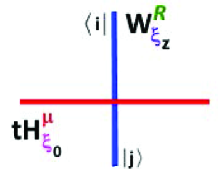
Figure 1: The operator $\mathcal{L}_{G}$ describing the matrix coupling between a horizontal ’t Hooft line (tH${}_{\xi_{0}}^{\mu}$ in red) at z=0 and a vertical Wilson line (W${}_{\xi_{z}}^{R}$ in blue) at z with incoming $\left\langle i\right|$ and out going $\left|j\right\rangle$ states. The spectral parameter z is interpreted in 4D CS theory as a point in the holomorphic plane.

As one of the main objective of this study is to give the full list of $\mathcal{L}_{G}$s, we think it interesting to: $\left(\mathbf{1}\right)$ describe here those basic quantities by using physical language and short paths for their properties. $\left(\mathbf{2}\right)$ emphasize the power of the QFT method of [1, 2] compared to the standard algebraic approach based on the Yangian algebra representations [35]. $\left(\mathbf{3}\right)$ draw an overview on the minuscule operators $\mathcal{L}_{G}$ and anticipate the construction by giving some results that will be derived rigorously later in this paper.

2.1 Families of minuscule $\mathcal{L}$-operators

We begin by recalling that, in addition to the symmetry Lie group G, the minuscule Lax-operators $\mathcal{L}_{G}$ of integrable 1D quantum spin chains and 2D integrable QFT systems are also classified by the minuscule coweights $\mu$ of finite dimensional Lie algebras. These minuscule coweights are quite well known in the mathematical literature on Lie group symmetries [36]; their useful properties for physical applications are as collected in the following Table 1.

$G$ minuscule$\ \mu$ Levi algebra $l_{\mu}$ $\dim$Rep nilpotent$\ \ n_{\pm}$ $A_{n}$ $\left.\begin{array}[]{c}\mu_{1}\\ \vdots\\ \mu_{k}\\ \vdots\\ \mu_{n}\end{array}\right.$ $\left.\begin{array}[]{c}sl_{1}\oplus A_{n-1}\\ \vdots\\ sl_{1}\oplus A_{k}\oplus A_{n-k}\\ \vdots\\ sl_{1}\oplus A_{n-1}\end{array}\right.$ $\left.\begin{array}[]{c}n+1\\ \vdots\\ \frac{\left(n+1\right)!}{k!\left(n+1-k\right)!}\\ \vdots\\ n+1\end{array}\right.$ $\left.\begin{array}[]{c}n_{\pm}\\ \vdots\\ k(n+1-k)_{\pm}\\ \vdots\\ n_{\pm}\end{array}\right.$ $B_{n}$ $\mu_{1}$ so${}_{2}\oplus B_{n-1}$ $2n$ $(2n-1)_{\pm}$ $C_{n}$ $\mu_{n}$ so${}_{2}\oplus A_{n-1}$ $2^{n}$ $\frac{1}{2}n(n+1)_{\pm}$ $D_{n}$ $\left.\begin{array}[]{c}\mu_{1}\\ \mu_{n-1}\\ \mu_{n}\end{array}\right.$ $\left.\begin{array}[]{c}so_{2}\oplus D_{n-1}\\ so_{2}\oplus A_{n-1}\\ so_{2}\oplus A_{n-1}^{\prime}\end{array}\right.$ $\left.\begin{array}[]{c}2n\\ 2^{n-1}\\ 2^{n-1}\end{array}\right.$ $\left.\begin{array}[]{c}(2n-2)_{\pm}\\ \frac{1}{2}n(n-1)_{\pm}\\ \frac{1}{2}n(n-1)_{\pm}\end{array}\right.$ $E_{6}$ $\left.\begin{array}[]{c}\mu_{1}\\ \mu_{6}\end{array}\right.$ $so_{2}\oplus D_{5}$ $\left.\begin{array}[]{c}27\\ \overline{27}\end{array}\right.$ $\left.\begin{array}[]{c}16_{\pm}\\ 16_{\pm}\end{array}\right.$ $E_{7}$ $\mu_{1}$ $so_{2}\oplus E_{6}$ $56$ $27_{\pm}$

Table 1: The list of the fundamental minuscule coweights $\mu$ of finite dimensional Lie algebras g. The Levi-decomposition of these algebras g with respect to the minuscule coweights is given by $\boldsymbol{n}_{-}\oplus\boldsymbol{l}_{\mu}\oplus\boldsymbol{n}_{+}$. Here, the $\boldsymbol{l}_{\mu}$ refers to the Levi-subalgebra and $\boldsymbol{n}_{\pm}$ to the nilpotent subalgebras. 

In this classification table, we have also reported the Levi-subalgebra $\boldsymbol{l}_{\mu}$ associated with the Lie algebra g underlying the symmetry group G. As well, we have given the nilpotent $\boldsymbol{n}_{\pm}$ subalgebras accompanying $\boldsymbol{l}_{\mu}$ and which turn out play an important role in the construction of the $\mathcal{L}_{G}^{\mu}$’s. From this global table, we learn amongst others that there exist five families of minuscule operators $\mathcal{L}_{G}^{\mu}$ denoted below as follows

$$\mathcal{L}_{A}^{\mu},$$

(2.1)

As exhibited on the Table 1, the four first operators $\mathcal{L}_{G}^{\mu}$ constitute four infinite families $\left\{\mathcal{L}_{G_{n}}^{\mu}\right\}$ labeled by the positive integer n (rank of G) and by the minuscule coweight $\mu$ of G. The fifth family in the Table 1 is finite, it concerns the exceptional $\mathcal{L}_{E_{6}}^{\mu}$ and $\mathcal{L}_{E_{7}}^{\mu}$. Because a given family may have more than one minuscule coweight; say $\mu_{k}$ labeled by an integer k, it results that the classification of the minuscule L-operators is given by two integers: $\left(\mathbf{i}\right)$ The rank $n_{G}$ of the gauge symmetry G_n with Lie algebra g_n. $\left(\mathbf{ii}\right)$ The number n_μ of minuscule coweights $\mu_{k}$ for each gauge symmetry G_n. 
Moreover, knowing that the minuscule coweights $\mu_{i}$ of finite Lie algebras are intimately related with their simple roots $\alpha_{i}$ as shown by the following duality relation

$$\mu_{i}.\alpha_{j}=\delta_{ij}$$ (2.2)

it follows that the $\mathcal{L}_{G}^{\mu}$’s can be put in correspondence with the Dynkin diagrams of the finite dimensional Lie algebras. In this regard, notice that as far as these Dynkin diagrams are concerned, those classical ones are given by infinite series A_n, B_n, C_n, D_n as depicted by the Figure 2. Similar comments can be said about the exceptional ones; especially the E₆ and E₇ which are relevant for the present study. These diagrams have nodes labeled by the simple roots $\alpha_{i}$ of G; and links $l_{ij}$ given by their non trivial intersections $\alpha_{i}.\alpha_{j}$.

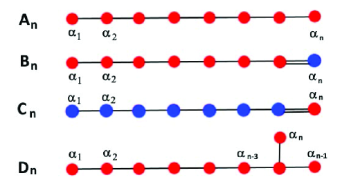
Figure 2: Classification of minuscule Lax operators in terms of the Dynkin diagrams of simple groups with minuscule coweights. Here, we have given the families $A_{n}=sl_{n+1},$ $B_{n}=so_{2n+1},$ $C_{n}=sp_{2n}$ and $D_{n}=so_{2n}$.

Notice also that formally speaking, the Dynkin diagrams considered here are graphic representations of the Cartan matrices $K_{ij}\left(G\right)$ of finite dimensional Lie algebras underlying gauge symmetries of QFT’s. These intersection matrices have particular integer entries with $\det K>0$; it reads in terms of the simple $\alpha_{i}$’s and their co-roots $\alpha_{j}^{\vee}$ as follows,

$$K_{ij}=\alpha_{i}^{\vee}.\alpha_{j}\qquad,\qquad\alpha_{i}^{\vee}=\frac{2}{\alpha_{i}.\alpha_{i}}\alpha_{i}.$$ (2.3)

where the scalar product $\alpha_{i}.\alpha_{i}$ refers to the length of the root. It is equal to 2 for the simply laced ADE Lie algebras; thus leading to a symmetric matrix $K_{ij}$. This feature does not hold for the non simply laced BC Lie algebras to be also investigated later.
Returning to the minuscule Lax operators $\mathcal{L}_{G}^{\mu}$; they are associated to the Dynkin diagrams $K_{ij}\left(G\right)$ whose minuscule node $\mu$ is omitted. As illustration, we give in the Figure 3 four examples regarding the cutting of the minuscule node in the Dynkin diagram. The first example is given by the omission of the first node $\alpha_{1}$ in the Dynkin diagram of sl$\left(9\right)$. This omission breaks the diagram $K\left(A_{8}\right)$ into two pieces given by

$$K\left(A_{8}\right)\rightarrow K\left(A_{1}\right)\oplus K\left(A_{7}\right)$$ (2.4)

with the isolated $\alpha_{1}$ corresponding to $K\left(A_{1}\right)$ and the seven others to $K\left(A_{7}\right)$. The second graph in the Figure 3 represents the omission of the fourth node $\alpha_{4}$ of the Dynkin diagram of sl$\left(9\right)$. This cutting leads to the breaking of $K\left(A_{8}\right)$ into three pieces with graphs as

$$K\left(A_{8}\right)\rightarrow K\left(A_{3}\right)\oplus K\left(A_{1}\right)\oplus K\left(A_{4}\right)$$ (2.5)

where the isolated $\alpha_{4}$ corresponds to $K\left(A_{1}\right)$ and the two other pieces to $K\left(A_{3}\right)$ and $K\left(A_{4}\right)$. These two ways of cutting the Dynkin diagram of $K\left(A_{8}\right)$ describe two different Lax operators $\mathcal{L}_{sl_{9}}^{\mu_{1}}$ and $\mathcal{L}_{sl_{9}}^{\mu_{4}}$ in the sl₉ theory. Regarding the other two graphic examples in the Figure 3, they concern the orthogonal so$\left(18\right)$ Lie algebra. The two cuttings correspond to the following graph decompositions

$$K\left(D_{9}\right) \rightarrow K\left(A_{1}\right)\oplus K\left(D_{8}\right)$$ (2.6)

$$K\left(D_{9}\right) \rightarrow K\left(A_{1}\right)\oplus K\left(A_{8}\right)$$ (2.7)

The first preserving the orthogonal structure of the broken diagram as shown by the $K\left(D_{8}\right)$ part. The second cutting destroys this feature since we have $K\left(A_{8}\right)$. As for the two previous example, eqs(2.6-2.7) describe two different Lax operators in so$\left(18\right)$ theory namely $\mathcal{L}_{so_{18}}^{\mu_{1}}$ and $\mathcal{L}_{so_{18}}^{\mu_{9}}$.

Figure 3: Four examples of graphs describing minuscule Lax operators. The first example concerns cutting the first node in A₈. The second example regards the cutting of the fourth minuscule node in A₈. These two graphs describe two different Lax operators. The third and the fourth graphs deals with Lax operators classified by D₉.

In conclusion, a general classification of the minuscule $\mathcal{L}_{G}^{\mu}$-operators describing crossing Wilson and ’t Hooft lines with unit electric and unit magnetic charges is given by the Table  2.

G_n $L_{G_{n}}^{\mu}$ $R$ of W${}_{\xi_{z}}^{R}$ simple roots # of $L_{G_{n}}^{\mu}$ $L_{G_{n}}^{\mu}$ -matrix A_n $L_{A_{n}}^{\mu_{k}}$ n $\alpha_{k}$    n eq(3.21) B_n $L_{B_{n}}^{\mu_{1}}$ 2n+1 $\alpha_{1}$    1 eq(3.30) C_n $L_{C_{n}}^{\mu_{n}}$ 2n $\alpha_{n}$    1 eq(3.33) D_n $L_{D_{n}}^{\mu_{1}},L_{D_{n}}^{\mu_{n-1}},L_{D_{n}}^{\mu_{n}}$ 2n $\alpha_{1},\alpha_{n-1},\alpha_{n}$    3 eqs(3.42-3.45-3.52) E₆ $L_{E_{6}}^{\mu_{1}},L_{E_{6}}^{\mu_{5}}$ 27 $\alpha_{1},\alpha_{5}$    2 eqs(3.56-3.58) E₇ $L_{E_{7}}^{\mu_{1}}$ 56 $\alpha_{6}$    1 eq(3.62)

Table 2: The full list of the minuscule Lax-operators $L_{G_{n}}^{\mu}$ in 4D Chern-Simons theory with gauge symmetry G and crossing Wilson and ’t Hooft lines having unit electric and magnetic charges. This basic list contains $\left(\mathbf{i}\right)$ four infinite families  given by the A_N-, B_N- C_N-, D_N- types. $\left(\mathbf{ii}\right)$ a finite exceptional subset having three elements: two equivalent E₆ and one E₇.

In this classification table, we have also given some useful informations like the electric charge of the Wilson line. We have even anticipated the results of this study by giving the links to the equations referring to the explicit expressions of the matrix representations of the Lax operators. These links to the $\mathcal{L}_{G_{n}}^{\mu}$ expressions are reported in the last column of the Table  2. It should be noted here that these realisations of the $\mathcal{L}_{G_{n}}^{\mu}$’s are derived with details in section 3. Notice moreover, that some of the results reported in this table are completely new, in particular those regarding $\mathcal{L}_{B}^{\mu}$ and $\mathcal{L}_{C}^{\mu}$ which are further investigated in sections 4 and 5.

2.2 Two approaches for constructing the $\mathcal{L}_{G_{n}}^{\mu}$’s

There are two basic approaches to construct the minuscule- Lax matrices of lower dimensional integrable systems. $\left(1\right)$ by using Yangian algebra representations [33]. $\left(2\right)$ by following the 4D Chern-Simons gauge theory approach. To fix the ideas, we review below the main lines of these two methods.

2.2.1 Algebraic Yangian approach

Here, we describe how the Yangian algebra naturally arises in the framework of the Yang- Baxter equation and its RLL representation whose its solution leads to the Lax-operator we are interested in. We start by recalling that the Yangian algebra is an infinite-dimensional Hopf algebra giving a simple example for quantum groups. Below, we consider the case of homogeneous rational spin chains with A-type symmetry and we illustrate through a short way the key steps for building the Lax-matrix $\mathcal{L}_{gl_{n}}\left(z\right)$ in this setup. We start from the usual Yang Baxter equation (YBE) given by [2]

$$R_{12}(z_{1}-z_{2})R_{13}(z_{1}-z_{3})R_{23}(z_{2}-z_{3})=R_{23}(z_{2}-z_{3})R_{13}(z_{1}-z_{3})R_{12}(z_{1}-z_{2})$$ (2.8)

where the R-matrix $R_{ij}(z_{i}-z_{j})$ depends only on the spectral parameter $z$. This matrix acts on the tensor product of the two vector spaces $V_{i}\otimes V_{j}$; it describes the coupling of two particles’ worldlines with inner spaces $V_{i}$ and $V_{j}.$ By setting $u=u_{1}-u_{3}$ and $v=u_{2}-u_{3}$ as well as $u-v=u_{1}-u_{2},$ we can bring the above YBE to the following form where the number of free parameters is reduced down: (u,v) instead of ($z_{1},z_{2},z_{3}$),

$$R_{12}(u-v)R_{13}(u)R_{23}(v)=R_{23}(v)R_{13}(u)R_{12}(u-v)$$ (2.9)

A quasi-classical solution to this equation is given by $R_{12}(z)=z\left(I+\frac{\hbar}{z}P_{12}\right)$ [2] where P₁₂ is the permutation operator acting like $P_{12}\left(z_{1}\otimes z_{2}\right)=z_{2}\otimes z_{1}.$ If we take two spaces in (2.9) as $V_{1}=\mathbb{C}^{n}$ and $V_{2}=\mathbb{C}^{n}$ and leave the third $V_{3}$ unspecified (auxiliary oscillator space), we recover the RLL relations that read as follows

$$R_{12}(u-v)L_{13}(u)L_{23}(v)=L_{23}(v)L_{13}(u)R_{12}(u-v)$$ (2.10)

Here, $L_{13}(u)$ and $L_{23}(v)$ are the Lax- matrices we are interested in; these are n$\times$n matrices constrained by the following commutation relations obtained after substituting with $R_{12}(z)=z\left(I+\frac{\hbar}{z}P_{12}\right).$

$$[L_{13}(u),L_{23}(v)]=\frac{\hbar}{u-v}P_{12}\left\{L_{13}(v)L_{23}(u)-L_{13}(u)L_{23}(v)\right\}$$ (2.11)

To get the above $L_{13}$ and $L_{23},$ we use the so-called monodromy matrix $M(z)$ with the following properties. It is a n$\times$n matrix operator function of the complex spectral parameter z that $\left(i\right)$ satisfies the RLL relations (2.10-2.11) and $\left(ii\right)$ allows to write down explicit commutation relations defining the Yangian algebra. By using the canonical matrix generator basis $\left\{\mathbf{e}_{ab}\right\}$ with 1$\leq a,b\leq$n, we can expand $M(z)$ as follows

$$M(z)=\sum_{a,b=1}^{n}M_{ab}(z)\otimes\mathbf{e}^{ab}$$ (2.12)

with matrix elements $M_{ab}(z)$ analytic in the complex spectral parameter z. These matrix entries have the following Laurent expansion [35]

$$M_{ab}(z)=M_{ab}^{{\small[0]}}+M_{ab}^{{\small[1]}}z^{-1}+M_{ab}^{{\small[2]}}z^{-2}+...$$ (2.13)

with $M_{ab}^{{\small[r]}}$ being the Laurent modes. Putting the expansion (2.13) into (2.11), we obtain the following system of commutation relations defining the Yangian algebra generated by the $M_{ab}^{[r]}$’s

$$[M_{ab}^{{\small[r]}},M_{cd}^{{\small[s]}}]=\sum_{q=1}^{\min(r,s)}\left(M_{cb}^{{\small[r+s-q]}}M_{ad}^{{\small[q-1]}}-M_{cb}^{{\small[q-1]}}M_{ad}^{{\small[r+s-q]}}\right)$$ (2.14)

with $\min(r,s)$ designating the minimal integer of the pair $\left(r,s\right)$. In what follows, we briefly describe the construction of Lax matrices of A-type by using the Yangian algebra Y(gl_n). This is an algebraic method that yields the oscillator realisation of the A-type Lax operator $\mathcal{L}(z)$. We consider the particular case where the expansion (2.13) ends at the first order, the $L(z)$ is therefore taken as

$$L(z)=M^{{\small[0]}}+\frac{1}{z}e^{ab}\otimes M_{ba}^{{\small[1]}}$$ (2.15)

with $M^{{\small[r]}}$ required to satisfy the Yangian algebra. We show below that the solutions of the RLL equations (2.14) are characterized by projectors $\Pi_{p}$ and the harmonic oscillator algebra encoded within $M_{ba}^{{\small[1]}}$. To construct the $M^{{\small[0]}}$ and $M^{{\small[1]}}$ matrices in (2.15), we use (2.14) expanded as

$$[M_{ab}^{{\small[0]}},M_{cd}^{{\small[0]}}]$$

(2.16)

The two first relations show that $M_{ab}^{{\small[0]}}$ matrix operator is a central element of the Yangian. So, it can be diagonalised by applying the automorphism $M_{ab}^{{\small[0]}}\rightarrow\tilde{M}_{ab}^{{\small[0]}}=B_{1}M_{ab}^{{\small[0]}}B_{2}$ where $B_{1}$ and $B_{2}$ are two invertible $n\times n$ matrices that act trivially in the quantum space $V_{3}$. The diagonal $\tilde{M}_{ab}^{{\small[0]}}$ reads in general like $q_{a}\tilde{M}_{aa}$ and eventually can be taken as follows

$$M_{k}^{[0]}=diag(\underset{p}{\underbrace{1,1,...,1}},\underset{(n-p)}{\underbrace{0,0,...,0}})$$ (2.17)

with label belonging $1\leq p\leq n.$ Notice that this choice corresponds to $M_{p}^{[0]}=\Pi_{p}$ describing projectors $\sum_{a=1}^{p}\left|a\right\rangle\left\langle a\right|$. For the special case where $p=n$, the matrix $M_{n}^{[0]}$ coincides with the identity $I_{n}.$ To determine $M^{[1]},$ we have to solve the two last relations of (2.16) with $M_{p}^{[0]}=\Pi_{p}$. To that purpose, we split the label $1\leq a,b\leq n$ like pairs $\left(\alpha,\dot{\alpha}\right)$ and $(\beta,\dot{\beta})$ with $1\leq\alpha,\beta\leq p$ and $p<\dot{\alpha},\dot{\beta}\leq n;$ and then think of $M^{[1]}$ as follows

$$M_{p}^{[1]}=\left(\begin{array}[]{cc}A_{\alpha\beta}&B_{\alpha\dot{\beta}}\\ C_{\dot{\alpha}\beta}&D_{\dot{\alpha}\dot{\beta}}\end{array}\right)$$ (2.18)

such that A, B, C, and D are respectively $p\times p,$ $p\times\left(n-p\right),$ $\left(n-p\right)\times p$ and $\left(n-p\right)\times\left(n-p\right)$ matrices. Next, we substitute (2.17) and (2.18) into the Yangian algebra representation (2.14), we obtain the following commutation relations constraining (2.18),

$$[A_{\alpha\beta},A_{\gamma\delta}]$$

(2.19)

and

$$[A_{\alpha\beta},B_{\gamma\dot{\delta}}]$$

(2.20)

as well as

$$[B_{\alpha\dot{\beta}},C_{\dot{\gamma}\delta}]=\delta_{\alpha\gamma}D_{\dot{\gamma}\dot{\beta}}$$ (2.21)

and

$$[D_{\dot{\alpha}\dot{\beta}},A_{\gamma\delta}]=[D_{\dot{\alpha}\dot{\beta}},B_{\gamma\dot{\delta}}]=[D_{\dot{\alpha}\dot{\beta}},C_{\dot{\gamma}\delta}]=0$$ (2.22)

The last relations (2.22) show that the $D_{\dot{\alpha}\dot{\beta}}$’s are central elements of the monodromy algebra. So, assuming $\det D\neq 0$ we can use the remaining freedom, used in putting $M_{ab}^{{\small[0]}}\rightarrow B_{1}M_{ab}^{{\small[0]}}B_{2}$ $=\left(\Pi_{p}\right)_{ab},$ to also put the $D_{\dot{\alpha}\dot{\beta}}$- matrix as given by $\delta_{\dot{\alpha}\dot{\beta}}.$ By substituting into (2.21), we end up with $[B_{\alpha\dot{\beta}},C_{\dot{\gamma}\delta}]=\delta_{\alpha\gamma}\delta_{\dot{\gamma}\dot{\beta}}$ that is convenient to rewrite like

$$[C_{\dot{\gamma}\delta}^{\prime},B_{\alpha\dot{\beta}}]=\delta_{\alpha\gamma}\delta_{\dot{\gamma}\dot{\beta}}$$ (2.23)

where we have set $C_{\dot{\gamma}\delta}^{\prime}=-C_{\dot{\gamma}\delta}$. In this way, the $B_{\alpha\dot{\beta}}$’s are interpreted as oscillator creators and $C_{\dot{\gamma}\delta}^{\prime}$ as the annihilators. Notice that this choice is due to the fact that the algebra (2.21) must admit a definition of a normalized trace over the oscillator algebras. This trace is different from the usual algebraic trace over gl(n); it is needed for the construction of transfer matrices and requires that $\det D\neq 0;$ see [35] for further details. Notice also that the Yangian algebra given by the commutation relations (2.19-2.22) is realised as the direct product

$$Y\left(gl_{p}\right)\simeq gl(p)\otimes\mathcal{H}^{\otimes p(n-p)}$$ (2.24)

Here, the $gl(p)$ algebra is generated by $A_{\alpha\gamma}$ and $\mathcal{H}^{\otimes p(n-p)}$ is the tensor product of $p(n-p)$ copies of the oscillator algebra (2.23) generated by the quantum harmonic oscillators $B_{\alpha\dot{\beta}},C_{\dot{\gamma}\delta}$. The generators $A_{\alpha\beta}$ solving the constraint relations (2.19-2.20) are realized as follows

$$A_{\alpha\beta}=\hat{J}_{\alpha\beta}-\sum_{\dot{\beta}=1}^{n-p}\left(B_{\alpha\dot{\beta}}C_{\dot{\beta}\beta}+\frac{1}{2}\delta_{\alpha\beta}\right)$$ (2.25)

with $\hat{J}_{\alpha\beta}$ being the transpose of $J_{\alpha\beta}.$ Therefore the Lax matrix constructed within the Yangian approach reads in terms of these oscillators as

$$L(z)=\left(\begin{array}[]{cc}z\delta_{\alpha\beta}+\hat{J}_{\alpha\beta}-\mathop{\displaystyle\sum}\limits_{\dot{\beta}=1}^{n-p}\left(B_{\alpha\dot{\beta}}C_{\dot{\beta}\beta}+\frac{1}{2}\delta_{\alpha\beta}\right)&B_{\alpha\dot{\beta}}\\ -C_{\dot{\alpha}\beta}&\delta_{\dot{\alpha}\dot{\beta}}\end{array}\right)$$ (2.26)

This Lax operator serves as an elementary building block for other solutions via the fusion procedure. They are used to build the Baxter operator and the transfer matrices using quantum harmonic oscillators; for details see [35] and references therein.

2.2.2 4D Chern Simons theory

Here, we describe the main lines of the 4D Chern-Simons gauge theory invariant under gauge symmetry groups G with Lie algebra g having at least one minuscule coweight $\mu$. The gauge symmetries considered below are as those given in the Table 2. First, we describe the gauge field action of the CS theory. Then, we give the RLL integrability equation formulated in terms of the Lax-operators and the R-matrix of Yang-Baxter equations.

Topological CS gauge field action:
The 4D Chern-Simons gauge theory is a topological QFT that was first obtained in [1]. Its gauge invariant field action $\mathcal{S}\left[\mathcal{A}\right]$ describing the dynamics of the gauge field $\mathcal{A}$ in the 4D space, that we take like $\boldsymbol{M}_{4}=\mathbb{R}^{2}\times\mathbb{CP}^{1},$ reads as follows

$$\mathcal{S}\left[\mathcal{A}\right]=\int_{\boldsymbol{M}_{4}}dz\wedge tr\Omega_{3}$$ (2.27)

where $\Omega_{3}$ is the CS 3-form

$$\Omega_{3}=\mathcal{A}\wedge d\mathcal{A}+\frac{2}{3}\mathcal{A}\wedge\mathcal{A}\wedge\mathcal{A}$$ (2.28)

To fix the ideas, we consider the family of gauge symmetry $G=SL_{N},$ a similar description is valid for the gauge symmetries given in the Table 2. In this case, the 1-form gauge potential is a function of the variables $\left(x,y;z\right)$ parameterising $\boldsymbol{M}_{4}$. It expands like $\mathcal{A}=t_{a}\mathcal{A}^{a}$ with $t_{a}$ standing for the generators of the Lie algebra $sl_{N}$ and $\mathcal{A}^{a}$ a partial gauge connection as follows [1]

$$\mathcal{A}^{a}=dx\mathcal{A}_{x}^{a}+dy\mathcal{A}_{y}^{a}+d\bar{z}\mathcal{A}_{\bar{z}}^{a}$$ (2.29)

The missing component $dz\mathcal{A}_{z}^{a}$ is killed by the factor $dz\wedge$ in the integral measure in (2.27). The equation of motion of the potential field $\mathcal{A}$ is given by the vanishing gauge curvature

$$\mathcal{F}_{2}=d\mathcal{A}+\mathcal{A}\wedge\mathcal{A}=0$$ (2.30)

This flat curvature property agrees with the topological nature of the CS theory (2.27), it indicates that the 4D CS gauge system is in the ground state with zero energy.

Line defects and observables:
To deform the topological ground state, we insert in the 4D CS gauge theory electrically charged Wilson and magnetically charged ’tHooft lines with magnetic charge given by the minuscule coweights. Interesting cases correspond to having interacting Wilson and ’tHooft lines. Examples of such couplings are given by crossing lines as depicted in the Figures 4-(a) and  4-(b) having an interpretation in terms of the Lax-operator and the RLL integrability equation.

Figure 4: On the left, the operator $\mathcal{L}$ describing the coupling between a ’t Hooft line at z=0 and a Wilson line at z with incoming $\left\langle i\right|$ and out going $\left|j\right\rangle$ states. On the right the graphic representation of RLL relations.

Let us comment the Figure 4-(a) while focussing on SL_N theory; we have:

$\left(\mathbf{1}\right)$

an electrically charged Wilson W^R with quantum states $\left|i\right\rangle$ generating a representation R of the gauge symmetry. This R is taken as the fundamental representation N of the gauge symmetry SL_N. The Wilson observable is given by the vertical blue line in the Figure 4-(a).

$\left(\mathbf{2}\right)$

a magnetically ’t Hooft line tH^μ with magnetic charge given by one of the N-1 minuscule coweights; say the first coweight $\mu_{1}$ in the Tables 1-2. The magnetic ’t Hooft observable is given by the horizontal red line in the Figure 4-(a).

The crossing matrix $\left\langle W^{\mathbf{R}},tH^{\mu}\right\rangle$ describing the coupling of the two topological lines is given by the Lax operator $\mathcal{L}_{sl_{N}}^{\mu}$ we are interested in here. It is obtained by solving the so-called RLL integrability equations briefly described here below.

2.2.3 RLL equation satisfied by the Lax operators

An interesting way to deal with the properties of the phase space $\mathcal{E}_{ph}$ of the classical Lax operator $\mathcal{L}$ is to use the graphic representation given by the Figures 4-(a) and (b). In the left picture of the this figure, we think of $\mathcal{L}_{sl_{N}}^{\mu}$ as a matrix operator $L_{i}^{j}=\left\langle i|\mathcal{L}_{sl_{N}}^{\mu}|j\right\rangle$ describing the crossing of a horizontal ’t Hoof line with a vertical Wilson line on which propagate $\left\langle i\right|$- and $\left|j\right\rangle$- states. The symplectic structure of the phase space of two operators $L_{j}^{r}\left(z\right)$ and $L_{l}^{s}\left(w\right),$ with spectral parameters z and w, is given by the RLL relations shown in the Figure 4. These integrability relations (which also hold at the quantum level) are due to the topological invariance of the 4D CS theory and read explicitly as follows [2],

$$R_{rs}^{ik}\left(z-w\right)L_{j}^{r}\left(z\right)L_{l}^{s}\left(w\right)=L_{r}^{i}\left(w\right)L_{s}^{k}\left(z\right)R_{jl}^{rs}\left(z-w\right)$$ (2.31)

Generally speaking, this tensorial relation gives the quantum integrability conditions of the topological system. The four rank object $R_{rs}^{ik}\left(z-w\right)$ is the usual R-operator used in the study of Yang- Baxter equation. At the leading order in the $\hbar$-expansion, we have $R_{jl}^{ik}(z)\simeq\delta_{j}^{i}\delta_{l}^{k}+\frac{\hbar}{z}c_{jl}^{ik}+O(h{{}^{2}})$ with $c_{jl}^{ik}$ standing for the double Casimir of the gauge symmetry. Putting back into 2.31, we obtain the following classical RLL relations

$$\left\{L_{j}^{i}\left(w\right),L_{l}^{k}\left(z\right)\right\}_{PB}=\frac{1}{z-w}\left[L_{l}^{i}\left(z\right)L_{j}^{k}\left(w\right)-L_{l}^{i}\left(w\right)L_{j}^{k}\left(z\right)\right]$$ (2.32)

where $\left\{\ast,\ast\right\}_{PB}$ stands for the Poisson Bracket.
One of the key points about eqs(2.31) is that they are solved by the following minuscule Lax operators

$$\mathcal{L}_{sl_{N}}^{\mu}\left(z\right)=e^{X}e^{\mu}e^{Y}$$ (2.33)

This solution first obtained in [25] concerns gauge symmetries $G$ having minuscule coweight $\mu$ (here $SL_{N}$). The $X$ and $Y$ are special matrices having the typical expansions $X=b^{\alpha}X_{\alpha}$ and $Y=Y^{\alpha}c_{\alpha}$ where the $X_{\alpha}$’s and $Y^{\alpha}$’s are generators of the nilpotent subalgebras $\boldsymbol{n}_{+}$ and $\boldsymbol{n}_{-}$ involved in the Levi-decomposition of the Lie algebra of the gauge symmetry with respect to the minuscule coweight [37]. This decomposition is given in this case by,

$$g$$

(2.34)

Another interesting point concerning (2.31) is that at the leading order in the $\hbar$-expansion of the R- matrix, one finds that the $\left(b,c\right)$ parameters involved in the expansions $b^{\alpha}X_{\alpha}$ and $Y^{\alpha}c_{\alpha}$ satisfy the usual Poisson bracket $\left\{b^{\alpha},c_{\beta}\right\}_{PB}=\delta_{\beta}^{\alpha}$ of the symplectic geometry. Then, this classical limit teaches us that: $\left(\mathbf{a}\right)$ the $\left(b^{\alpha},c_{\alpha}\right)$ are nothing but the Darboux coordinates (classical harmonic oscillators) of the phase space of the L-operator. $\left(\mathbf{b}\right)$ the particular solution (2.33) gives an oscillator realisation of the Lax operators like the ones obtained from the Yangian based method of integrable quantum spin chains.

3 Minuscule $\mathcal{L}_{G}$ from CS theory: the full list

In this section, we introduce and develop a suitable operator basis (method of projectors) to deal with the explicit calculation of the Lax operator of integrable spin chain satisfying the RLL equation. We begin by describing the main steps of the derivation of the minuscule Lax operators $\mathcal{L}_{G}$ for gauge symmetries G given by the A_N, B_N, C_N, D${}_{N},$ E₆, E₇ families. Then, we give the full list of the explicit oscillator realisations of these $\mathcal{L}_{G}$s. This list gives a unified description of all minuscule $\mathcal{L}_{G}$s and presents new results concerning the non simply laced families $\mathcal{L}_{B}^{\mu_{1}}$ and $\mathcal{L}_{C}^{\mu_{N}}$. Other aspects regarding the relationships between the various $\mathcal{L}_{G}$’s and discrete symmetries are also studied in order to complete the investigation of minuscule $\mathcal{L}_{G}$s.

3.1 The calculation of $\mathcal{L}_{G}$: method of projectors

Here we give a suitable calculation method to work out the explicit matrix-representation of the minuscule Lax operator $\mathcal{L}_{G}$. We term this approach as the method of projectors; for the motivation behind this terminology, we refer to eqs(3.1-3.4) given below.
We start by recalling that the minuscule Lax operator $\mathcal{L}_{G}$ is given by (2.33) namely $\mathcal{L}_{G}^{\mu}=e^{X}z^{\mu}e^{Y}$. This formula involves three Lie algebraic objects that we comment below:

• The adjoint action $\mathbf{\mu}$ of the minuscule coweight; it belongs to the Lie sub-algebra $\boldsymbol{l}_{\mu}$ of Table 1. This $\boldsymbol{l}_{\mu}$ results from the Levi- decomposition of the Lie algebra $g$ underlying the gauge symmetry which decomposes like $g=\boldsymbol{n}_{-}\oplus\boldsymbol{l}_{\mu}\oplus\boldsymbol{n}_{+}$.

• The two $X$ and $Y$ operators are nilpotent matrices evaluated in the nilpotent sub-algebras $\boldsymbol{n}_{+}$ and $\boldsymbol{n}_{-}$ following the Levi- decomposition. The intrinsic properties of $X$ and $Y$ carry data on the electric charge of the Wilson line and the magnetic charge of the ’t Hooft line.

To determine the explicit expression of $\mathcal{L}_{G}$, we have to first find the matrix representations of these three objects; then use them to calculate $e^{X}z^{\mathbf{\mu}}e^{Y}$.
So, given a 4D Chern-Simons theory with gauge symmetry G, we can determine the expression of the minuscule $\mathcal{L}_{G}$ solving the RLL equation (2.31) by using (2.33). This is done in three steps as described below:

$\mathbf{1)}$ Working out the adjoint action of $\mu$
The adjoint action of the minuscule coweight is a charge operator representation $\mathbf{\mu}$ acting on the Hilbert space $\mathcal{H}$ of the Wilson line interacting with the ’t Hooft defect. For concreteness, we denote the vector basis of the space $\mathcal{H}$ of the quantum states by kets $\left|i\right\rangle$ as in the Figure 4-(a). These quantum states generating the representation $\mathbf{R}_{G}$ of the gauge symmetry run along the Wilson line. This representation $\mathbf{R}_{G}$ will be thought of below as given by the fundamental representation of the gauge symmetry.
Because of the Levi-decomposition of the gauge symmetry G, the representation $\mathbf{R}_{G}$ splits in turns into a sum of representations $\mathbf{R}_{a}^{\boldsymbol{l}_{\mu}}$ of the Levi-subalgebra $\boldsymbol{l}_{\mu}$. Formally, we have

$$\mathbf{R}_{G}=\oplus_{a}\mathbf{R}_{a}^{\boldsymbol{l}_{\mu}}$$ (3.1)

The charge operator $\mathbf{\mu}$ is effectively given by these representations; it explicitly reads in terms of projectors $\varrho_{{}_{\mathbf{R}_{a}}}:\mathbf{R}_{G}\rightarrow\mathbf{R}_{a}$ as follows

$$\mathbf{\mu}=\sum_{\mathbf{R}_{a}}m_{{}_{\mathbf{R}_{a}}}\varrho_{{}_{\mathbf{R}_{a}}}$$ (3.2)

with

$$\sum_{\mathbf{R}_{a}}\varrho_{{}_{\mathbf{R}_{a}}}=I_{id}\qquad,\qquad\varrho_{{}_{\mathbf{R}_{a}}}\varrho_{{}_{\mathbf{R}_{b}}}=\delta_{ab}\varrho_{{}_{\mathbf{R}_{a}}}$$ (3.3)

For a traceless representation $\mathbf{R}_{G},$ we get the following constraint relation on the Levi-charges $m_{{}_{\mathbf{R}_{a}}}$ carried by a representation $\mathbf{R}_{a}^{\boldsymbol{l}_{\mu}}$.

$$\sum_{\mathbf{R}_{a}}m_{{}_{\mathbf{R}_{a}}}=0$$ (3.4)

$\mathbf{2)}$ Solving the conditions of the Levi-decomposition
Once the adjoint action $\mathbf{\mu}$ is known, we move to determining the realisation of the $X$ and $Y$ matrices in the Hilbert space of quantum states of the Wilson/’t Hooft lines. They are obtained by $\left(i\right)$ using the expansions $X=b^{\alpha}X_{\alpha}$ and $Y=c_{\alpha}Y^{\alpha}$; and $\left(ii\right)$ solving the Levi-conditions

$$\left[\mathbf{\mu},X_{\alpha}\right]$$

(3.5)

In these Levi-constraint relations, Each generator $X_{\alpha}$ of $\boldsymbol{n}_{+}$ carries a positive unit charge $+1$ and each generator $Y^{\alpha}$ of $\boldsymbol{n}_{-}$ carries a negative unit charge $-1.$

$\mathbf{3)}$ Calculating the L-operator $\mathcal{L}_{G}$ as a bi-polynom in $\mathbf{X}$ and $\mathbf{Y}$
Because of the nilpotency property of the $X_{\alpha}$ and $Y^{\alpha}$ generators of $\boldsymbol{n}_{\pm}$ and commuting properties like $\left[X_{\alpha},X_{\beta}\right]=0$; the $X$ and $Y$ are as well nilpotent. So, there should exist an order n and an order m such that $X^{k+1}=0$ and $Y^{l+1}=0.$ In fact the two orders are equal $k=l$ because of the duality between $X$ and $Y$. So, the exponentials $e^{X}$ and $e^{Y}$ have finite expansions of the form $e^{Z}=I+Z+...\frac{1}{k!}Z^{k}.$ Putting this back into $e^{X}z^{\mu}e^{Y},$ we end up with the oscillator realisation of $\mathcal{L}_{G}$ given by

$$\mathcal{L}_{G}=\sum_{n,m}\frac{1}{n!m!}X^{n}z^{\mu}Y^{m}$$ (3.6)

where $X=b^{\alpha}X_{\alpha}$ and $Y=c_{\beta}Y^{\beta}$ as well as

$$z^{\mu}=\sum z^{m_{a}}\varrho_{{}_{\mathbf{R}_{a}}}$$ (3.7)

Finally, using the properties of the projectors $\varrho_{{}_{\mathbf{R}_{a}}}$, we can present $\mathcal{L}_{G}$ by a matrix $L_{ab}$ given by

$$L_{ab}^{G}=\varrho_{{}_{\mathbf{R}_{a}}}\mathcal{L}_{G}\varrho_{{}_{\mathbf{R}_{b}}}$$ (3.8)

3.2 The A_N operator family: $L_{ab}^{A_{N}}$

Here, we give an example to explain the above steps of the calculation of the Lax-matrix $L_{ab}^{G}$ (3.8). We consider the case of a 4D Chern-Simons theory with gauge symmetry SL$\left(N\right)$ in presence of an electrically charged Wilson line W with fundamental electric charge $\lambda_{1}$ as depicted by the Figure 4-(a). this W-line crosses a magnetically charged ’t Hooft line with magnetic charge given by the minuscule coweight $\mu_{1}$.
As far as the Lie algebra $A_{N-1}\simeq sl_{N}$ of the gauge symmetry SL$\left(N\right)$ is concerned, it is interesting to recall some useful mathematical features that we collect in the following table (3.9).

algebra $${\small A}_{N-1}$$

dim

rank

roots

Cartan H_i

step

(3.9)

       

These properties regard the Levi-decomposition of $sl_{N}$ with respect to the minuscule coweight $\mu_{1}$ namely

$$sl_{N}\rightarrow sl_{1}\oplus sl_{N-1}+\boldsymbol{n}_{+}\oplus\boldsymbol{n}_{-}$$ (3.10)

The adjoint action of the minuscule coweights $\mu_{1}$ is therefore given by

$$\mathbf{\mu}_{1}=\frac{N-1}{N}\left|1\right\rangle\left\langle 1\right|-\frac{1}{N}\sum_{i=2}^{N}\left|i\right\rangle\left\langle i\right|$$ (3.11)

The generators $X_{i}$ and $Y^{i}$ of the nilpotent sub-algebras $\boldsymbol{n}_{+}$ and $\boldsymbol{n}_{-}$ solving the Levi- constraint relations are given by

$$X_{i}$$

(3.12)

The Lax matrix representing the L-operator reads as follows

$$\mathcal{L}_{A_{N}}=\left(\begin{array}[]{cc}z^{\frac{N-1}{N}}+z^{-\frac{1}{N}}\mathbf{b}^{T}\mathbf{c}&z^{-\frac{1}{N}}\mathbf{b}^{T}\\ z^{-\frac{1}{N}}\mathbf{c}&z^{-\frac{1}{N}}I_{N-1}\end{array}\right)$$ (3.13)

with $\mathbf{b}^{T}=\left(b_{1},...,b_{N-1}\right)$ and $\mathbf{c}=\left(c_{1},...,c_{N-1}\right)^{T}.$ By multiplying this matrix with the factor $z^{\frac{1}{N}}$, we get the familiar Lax-matrix obtained in the quantum spin chain literature [27], namely

$$\mathcal{\tilde{L}}_{A_{N}}=\left(\begin{array}[]{cc}z^{N-1}+\mathbf{b}^{T}\mathbf{c}&\mathbf{b}^{T}\\ \mathbf{c}&I_{N-1}\end{array}\right)$$ (3.14)

3.3 The full list of minuscule L-operators

The list of the full set $\mathfrak{M}$ of minuscule Lax operators with unit charges is infinite. It contains five sub-families given by the four classical series A_N, B_N, C_N, D_N and the exceptional finite E${}_{6},$ E₇. These sub-families o the set $\mathfrak{M}$ of L-operators are revisited below separately in the given ordering.

3.3.1 A_N-1- type operators $\mathcal{L}_{A}$

First we give the general form of the Lax-matrices $\mathcal{L}_{A_{N-1}}^{\mu_{k}}$ for generic fundamentals coweights $\mu_{k}$ with label $1\leq k\leq N-1$ and label $N-1$ being the rank of $A_{N-1}$. Then, we comment the exotic property of the $A_{N-1}$-family regarding the CS theory with gauge symmetry SL${}_{2M};$ that is $N=2M$.

I) Generic formula for $\mathcal{L}_{A_{N-1}}^{\mu_{k}}$
We start by recalling that the A_N-1 Lie algebra series has $N-1$ minuscule coweights $\mathbf{\mu}_{k}$ labeled by $1\leq k\leq N-1.$ These coweights are expressed in terms of the weight vector basis $\left\{e_{i}\right\}_{1\leq i\leq N}$ like

$$(\text{ }\underbrace{\frac{N-k}{N},...,\frac{N-k}{N}}_{k}\text{ };\text{ }\underbrace{-\frac{k}{N},...,-\frac{k}{N}}_{N-k}\text{ })$$ (3.15)

The unit vectors $e_{i}$ in the weight vector basis are now on denoted by the kets $\left|i\right\rangle$ and their duals are represented by the bras $\left\langle i\right|$. The Levi-decomposition of the sl$\left(N\right)$ Lie algebra with respect to $\mathbf{\mu}_{k}$ is given by

$$sl_{N}\rightarrow sl_{1}\oplus sl_{k}\oplus sl_{N-k}\oplus\boldsymbol{n}_{+}\oplus\boldsymbol{n}_{-}$$ (3.16)

with $\boldsymbol{n}_{\pm}=k\left(N-k\right)_{\pm}$. The adjoint action of the minuscule coweight is realised in terms of the $\left|i\right\rangle$ weight vectors as

$$\mathbf{\mu}_{k}=\left(1-\frac{k}{N}\right)\mathop{\displaystyle\sum}\limits_{i=1}^{k}\left|i\right\rangle\left\langle i\right|-\frac{k}{N}\mathop{\displaystyle\sum}\limits_{i=k+1}^{N}\left|i\right\rangle\left\langle i\right|$$ (3.17)

For later use, we will also use the convenient notation

$$\mathbf{\mu}_{k}=\left(1-\frac{k}{N}\right)\mathop{\displaystyle\sum}\limits_{i=1}^{k}\left|i\right\rangle\left\langle i\right|-\frac{k}{N}\mathop{\displaystyle\sum}\limits_{i=1}^{N-k}\left|\bar{\imath}\right\rangle\left\langle\bar{\imath}\right|$$ (3.18)

where we have set $\bar{\imath}=N+1-i.$ Notice that $i+\bar{\imath}=N+1$ such that

$$i$$

(3.19)

The charge operator (3.18) is traceless, $Tr\left(\mathbf{\mu}_{k}\right)=0$. We often refer to $\mathbf{\mu}_{k}$ as the Levi-Charge operator. The $k\left(N-k\right)$ operators generating the nilpotent algebras $\boldsymbol{n}_{\pm}$ are now denoted like $X_{ia}^{\mu_{k}}$ and $Y_{\mu_{k}}^{ia}.$ The explicit representation of these generators in the Hilbert space of the crossing lines is obtained by solving the Levi-constraint relations (3.5) reading as follows

$$X_{i\bar{a}}^{\mu_{k}}$$

(3.20)

with labels as $1\leq i\leq k$ and $k<a\leq N$ or equivalently $\bar{N}\leq\bar{a}<\bar{k}$. The Lax- matrix associated with the coweight $\mu_{k}$ is obtained by substituting the expansions $X=b^{i\bar{a}}X_{i\bar{a}}^{\mu_{k}}$ and $X=Y^{\bar{a}i}c_{\bar{a}i}$ into $e^{X}z^{\mathbf{\mu}_{k}}e^{Y}$. We get

$$\mathcal{L}_{A_{N}}^{\mu_{k}}=\left(\begin{array}[]{cc}z^{\frac{N-k}{N}}I_{k}+z^{-\frac{k}{N}}\mathbf{bc}&z^{-\frac{k}{N}}\mathbf{b}\\ z^{-\frac{k}{N}}\mathbf{c}&z^{-\frac{k}{N}}I_{N-k}\end{array}\right)$$ (3.21)

Here, the $\mathbf{b}$ and $\mathbf{c}$ refer to the k$\left(N-k\right)$ oscillators $\mathbf{b}^{i\bar{a}}$ and k$\left(N-k\right)$ oscillators $\mathbf{c}_{\bar{a}i}$ given by

$$\mathbf{b}^{ia}=\left(\begin{array}[]{ccc}b^{1\bar{N}}&\cdots&b^{1\overline{k+1}}\\ \vdots&\ddots&\vdots\\ b^{k\bar{N}}&\cdots&b^{k\overline{k+1}}\end{array}\right)\qquad,\qquad\mathbf{c}_{ai}=\left(\begin{array}[]{ccc}c_{\bar{N}k}&\cdots&c_{\bar{N}1}\\ \vdots&\ddots&\vdots\\ c_{\overline{k+1}k}&\cdots&c_{\overline{k+1}1}\end{array}\right)$$ (3.22)

II) Automorphism symmetries of $\mathcal{L}_{A_{N-1}}^{\mu_{k}}\newline$We begin by noticing that the examination of eq(3.18) reveals a remarkable property of the coweights $\mathbf{\mu}_{k}$. In fact, by making the following $\mathbb{Z}_{2}$ discrete change,

$$\mathbb{Z}_{2}:\left.\begin{array}[]{ccc}k&\rightarrow&N-k\\ \left|i\right\rangle&\rightarrow&\left|\bar{\imath}\right\rangle\end{array}\right.$$ (3.23)

we learn that the corresponding operator charge operators transform as $\mathbf{\mu}_{N-k}\rightarrow-\mathbf{\mu}_{k}.$ This symmetry property indicates that eq(3.21) hides an interesting symmetry property explicitly exhibited by the case where $N=2M$. This symmetry property has an interpretation in the language of $A_{N-1}$ representations and their adjoint conjugates. It also allows to engineer new $\mathcal{L}$-operators from (3.21) inspired by Dynkin diagram folding ideas. We will see later that the fixed point of the folding of (3.21) under the above $\mathbb{Z}_{2}$ symmetry reading as

$$\mathcal{L}_{A_{2M-1}}^{\mu_{M}}=\left(\begin{array}[]{cc}z^{\frac{1}{2}}I_{M}+z^{-\frac{1}{2}}\mathbf{bc}&z^{-\frac{1}{2}}\mathbf{b}\\ z^{-\frac{1}{2}}\mathbf{c}&z^{-\frac{1}{2}}I_{M}\end{array}\right)$$ (3.24)

gives precisely the L-operators $\mathcal{L}_{C_{M}}^{\mu}$ of the symplectic family $SP\left(2M\right)$. In this regard, notice the following properties:

$\left(\mathbf{1}\right)$

For the 4D Chern-Simons theory with gauge symmetry $G=SL\left(2M\right),$ the Lax- matrix $\mathcal{L}_{A_{2M-1}}^{\mu_{k}}$ has four main blocks: $\left(i\right)$ two diagonal blocks of dimensions k$\times$k and (2M-k)$\times$(2M-k) and $\left(ii\right)$ two off diagonal with dimensions k$\times$(2M-k) and (2M-k)$\times$k. For the particular case where $k=M$, all the four above blocks are iso-dimensional. This iso-dimensional property corresponding to the fixed point of the $\mathbb{Z}_{2}$-symmetry (3.23) is nothing but the $\mathbb{Z}_{2}$-outer-automorphism of the Dynkin diagram of SL$\left(2M\right)$ as depicted by the Figure 5 for the example of SL$\left(4\right)$.

Figure 5: On the left, the Dynkin diagram of the Lie algebra A${}_{3}.$ It has a $\mathbb{Z}_{2}$- outer-automorphism symmetry leaving one node fixed (in magenta color). On the right, the Dynkin diagram of the symplectic Lie algebra C₂. It is obtained by folding A₃ under $\mathbb{Z}_{2}$.

$\left(\mathbf{2}\right)$

  For the sub-family of the 4D CS gauge symmetries given by $SL\left(2M\right)$, the Levi-decomposition of its underlying Lie algebra reads as follows

$$sl_{2M}\rightarrow sl_{1}\oplus sl_{M}\oplus sl_{M}\oplus M_{+}^{2}\oplus M_{-}^{2}$$ (3.25)

This can be checked from the calculation of the ranks and the dimensions of both sides of (3.25). If thinking of this gauge symmetry in terms of the semi-simple $gl_{2M}$, its 4M² dimensions split like $M^{2}+M^{2}+M^{2}+M^{2}.$ For the special coweight $\mu_{k}$ with $k=M$, eqs(3.18-3.20) read as follows

$$\mathbf{\mu}_{M}=\frac{1}{2}\mathop{\displaystyle\sum}\limits_{i=1}^{M}\left(\left|i\right\rangle\left\langle i\right|-\left|\bar{\imath}\right\rangle\left\langle\bar{\imath}\right|\right)$$ (3.26)

and

$$X_{i\bar{j}}$$

(3.27)

The Lax-matrix (3.21) associated with the coweights $\mathbf{\mu}_{M}$ is given by (3.24). We will reconsider these relations when we study the construction of the Lax-matrix for 4D Chern-Simons theory with symplectic$SP_{2M}$ gauge symmetry (see section 5).

3.3.2 B-type operators $\mathcal{L}_{B}$: new result

Now, we consider the case where the gauge symmetry of the 4D Chern-Simons is given by SO_2N+1. As shown in Table 1, this gauge symmetry group has one minuscule coweight $\mathbf{\mu}_{1}$ dual to the simple root $\alpha_{1}$. To get more insight into the algebraic properties of $\mathcal{L}_{B},$ we recall some useful properties of the $B_{N}$ gauge symmetry. The SO_2N+1 has $2N^{2}$ roots, half of them are positive and denoted as $+\alpha_{ij}^{\pm}$ where $i,j=1,...,N$. The negative ones are given by the opposites that read as $-\alpha_{ij}^{\pm}$. These $\pm\alpha_{ij}^{\pm}$’s have two lengths: $N\left(2N-1\right)$ of them have length 2 realised in terms of $N$ weight vector basis $\left\{e_{i}\right\}$ like $\pm\left(e_{i}\pm e_{j}\right)$ with $i\neq j.$ The remaining $N$ others have length 1; they are given by $\pm\alpha_{ii}^{+}$ and are realised as $\pm e_{i}.$ The $N$ simple roots $\alpha_{i}$ of the Lie algebra of SO_2N+1 are given by: $\left(\mathbf{a}\right)$ $\alpha_{i}=e_{i}-e_{i+1}$ for $i=1,...,N-1$ having length 2. $\left(\mathbf{b}\right)$ $\alpha_{N}=e_{N}$ having length 1. In this basis, the minuscule coweight is given by $\mu_{1}=e_{1}$ obeying $\mu_{1}.\alpha_{1}=1.$
The Levi-decomposition of the Lie algebra of $SO_{2N+1}$ reads as $so_{2}\oplus so_{2N-1}\oplus\boldsymbol{n}_{\pm}$ with nilpotent sector as $\boldsymbol{n}_{\pm}=(2N-1)_{\pm}$. It corresponds to cutting the first node $\alpha_{1}$ in the Dynkin diagram of $B_{N}\simeq so_{2N+1}$ as depicted by the Figure 6.

Figure 6: Dynkin Diagram of B_N illustrated for the example where $N=6$. By cutting the first node $\alpha_{1},$ one ends with the Diagram associated with the Dynkin diagram of the B_N-1 subalgebra and a free node $\alpha_{1}$ capturing data on the SO₂ Levi-charge and the nilpotent subalgebras.

The adjoint action of the minuscule coweight $\mathbf{\mu}$ is given by

$$\mathbf{\mu}=\frac{1}{2}\varrho_{+}+q\mathop{\displaystyle\sum}\limits_{i=1}^{2N-1}\varrho_{i}-\frac{1}{2}\varrho_{-}$$ (3.28)

where we have for commodity inserted the central terms although $q=0;$ this is because it contributes to $z^{\mathbf{\mu}}.$ The $\varrho_{\pm}=\left|\pm\right\rangle\left\langle\pm\right|$ and the $\varrho_{i}=\left|i\right\rangle\left\langle i\right|$ are projectors. The matrix realisation of the $X_{i}$ and $Y^{i}$ generators of the nilpotent algebras are as follows

$$X_{i}$$

(3.29)

We also have the expansions $X=b^{i}X_{i}$ and $Y=c_{i}Y^{i}$. These relations will be discussed further in section 4. The explicit matrix realisation of the Lax operator $\mathcal{L}_{B}^{\mu_{1}}$ is also derived in section 4; it reads as follows

$$\mathcal{L}_{B}^{\mu_{1}}=\left(\begin{array}[]{lll}z+\mathbf{b}^{T}\mathbf{c+}\frac{1}{4}z^{-1}\mathbf{b}^{2}\mathbf{c}^{2}&\mathbf{b}^{T}-\frac{1}{2}z^{-1}\mathbf{b}^{2}\mathbf{c}^{T}&\frac{1}{2}z^{-1}\mathbf{b}^{2}\\ \mathbf{c-}\frac{1}{2}z^{-1}\mathbf{c}^{2}\mathbf{b}&I_{2N-1}+z^{-1}\mathbf{b}^{T}\mathbf{c}&-z^{-1}\mathbf{b}\\ \frac{1}{2}z^{-1}\mathbf{c}^{2}&-z^{-1}\mathbf{c}^{T}&z^{-1}\end{array}\right)$$ (3.30)

with $\mathbf{b}^{2}=b^{i}\delta_{ij}b^{j}$ and $\mathbf{c}^{2}=c_{i}\delta^{ij}c_{j}$ as well as $\mathbf{b}^{T}\mathbf{.c}=b^{i}c_{i}$. In the basis $\left\{\left|+\right\rangle,\left|i\right\rangle,\left|-\right\rangle\right\},$ the entries of the $X$ and $Y$ are respectively given by $(2N+1)\times 1$ and $1\times(2N+1)$ matrix oscillators given by $\mathbf{b}^{T}=\left(0,b_{1},\cdots,b_{2N-1},0\right)$ and $\mathbf{c}^{T}=\left(0,c_{1},\cdots,c_{2N-1},0\right).$

3.3.3 C-type operators $\mathcal{L}_{C}$: new result

In this case, the gauge symmetry of the 4D Chern-Simons is given by the symplectic group SP_2N having rank N and dimension $2N^{2}+N$ thought of below as $N^{2}+N(N+1).$ It has one minuscule coweight $\mu_{N}$ dual to the simple root $\alpha_{N}$. In this regard, recall that $SP_{2N}$ has $2N^{2}$ roots, half of them are positive and the others are negative roots. These roots are realised in terms of the $e_{i}$ weight vectors as $\pm\alpha_{ij}^{\pm}=\pm e_{i}\pm e_{j}$ $(1\leq i<j\leq N)$ and $\pm 2e_{i}$ for $1\leq i\leq N.$ The $N$ simple roots $\alpha_{i}$ of SP_2N are given by $e_{i}-e_{i+1}$ for $i=1,...,N-1$ having length 2; and $\alpha_{N}=2e_{N}$ with length 4. In this basis, the minuscule coweight is given by $\mu_{N}=\frac{1}{2}(e_{1}+...+e_{N})$; it describes the symplectic fundamental representation with dimension 2N.
The Levi-decomposition of the Lie algebra of the symplectic gauge symmetry reads as $so_{2}\oplus sl_{N}\oplus\boldsymbol{n}_{\pm}$ with nilpotent algebras $\boldsymbol{n}_{\pm}=\frac{1}{2}N\left(N+1\right)_{\pm}$ which are given by the symmetric representations of $sl_{N}$ and its conjugate. This corresponds to cutting the first node $\alpha_{1}$ in the Dynkin diagram of $B_{N}\simeq so_{2N+1}$ as depicted by the Figure 7.

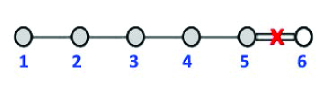
Figure 7: Dynkin Diagram of C_N illustrated for the example where $N=6$. By cutting the first node $\alpha_{N},$ one ends with the Diagram associated with the Dynkin diagram of the A_N-1 subalgebra and a free node $\alpha_{N}$ capturing data on the SO₂ Levi-charge and the nilpotent subalgebras.

The adjoint action $\mathbf{\mu}$ of the minuscule coweight and the matrix realisation of the $X_{i\bar{\imath}},X_{\left[i\bar{j}\right]}$ and $Y^{\bar{\imath}i},Y^{\left[\bar{\imath}j\right]}$ generators of the nilpotent algebras $\boldsymbol{n}_{\pm}$ are given by

$$X_{i\bar{\imath}}$$

(3.31)

and

$$\mathbf{\mu}=\frac{1}{2}\sum_{i=1}^{N}\varrho_{i}-\frac{1}{2}\sum_{\bar{\imath}=\bar{1}}^{\bar{N}}\bar{\varrho}_{i}$$ (3.32)

The Lax- matrix operator $\mathcal{L}_{C}^{\mu_{N}}$ is explicitly derived in section 5; it reads as follows

$$\mathcal{L}_{C}^{\mu_{N}}=\left(\begin{array}[]{cc}z^{\frac{1}{2}}I_{N}+z^{-\frac{1}{2}}XY&z^{-\frac{1}{2}}X\\ z^{-\frac{1}{2}}Y&z^{-\frac{1}{2}}I_{N}\end{array}\right)$$ (3.33)

This Lax-matrix must be compared with (3.24). The entries of X and Y matrices in the basis $\left\{\left|i\right\rangle,\left|\bar{\imath}\right\rangle\right\}$ are given by

$$X=\left(\begin{array}[]{ccc}b_{1\bar{N}}&\cdots&b_{1\bar{1}}\\ \vdots&\ddots&\vdots\\ b_{N\bar{N}}&\cdots&b_{N\bar{1}}\end{array}\right)\qquad,\qquad Y=\left(\begin{array}[]{ccc}c_{\bar{N}1}&\cdots&c_{\bar{N}N}\\ \vdots&\ddots&\vdots\\ c_{\bar{1}1}&\cdots&c_{\bar{1}N}\end{array}\right)$$ (3.34)

Multiplying (3.33) by $z^{1/2}$, we obtain

$$\mathcal{\tilde{L}}_{C}^{\mu_{N}}=\left(\begin{array}[]{cc}zI_{N}+XY&X\\ Y&I_{N}\end{array}\right)$$ (3.35)

3.3.4 D-type operators revisited

For the case of the 4D Chern-Simons with gauge symmetry SO_2N+1; we have three minuscule coweights $\mu_{1},\mu_{N-1}$ and $\mu_{N}$ as shown in Table 1. Therefore, we have three types of minuscule Lax operators.

$$\mathcal{L}_{D}^{\mu_{1}},\qquad\mathcal{L}_{D}^{\mu_{N-1}},\qquad\mathcal{L}_{D}^{\mu_{N}}$$ (3.36)

To get more insight into the algebraic structure underlying these L-operators, it is interesting to recall useful relations: $\left(\mathbf{1}\right)$ the SO_2N has $2N^{2}$ roots, half of them are positive and the other half are negative. These roots have length 2 and are realised in the weight vector basis $\left\{e_{1},...,e_{N}\right\}$ like $\pm\left(e_{i}\pm e_{j}\right)$ with $1\leq i<j\leq N.$ The N simple roots $\alpha_{i}$ of SO_2N are given by

$$\alpha_{i}$$ for

(3.37)

In this basis, the minuscule coweights, satisfying $\mu_{1}.\alpha_{1}=1$ and $\mu_{N-1}.\alpha_{N-1}=1$ as well as $\mu_{N}.\alpha_{N}=1,$ are given by

$$\mu_{1}$$

(3.38)

The Levi-decompositions of the so_2N Lie algebra with respect to the three minuscule coweights are as follows; see also the Table 1,

$$\mu_{1}$$ :

:

:

(3.39)

The three Lax-matrices (3.36) corresponding to these three minuscule coweights are described below.

$\mathbf{I)}$ Vectorial coweight: $so_{2N}\rightarrow so_{2}\oplus so_{2N-2}\oplus\left(2N-2\right)_{\pm}$
In the decomposition of so_2N with respect to $\mu_{1}$ corresponding to cutting the node $\alpha_{1}$ in the Dynkin diagram of the Figure 8, the electric charge of Wilson line is given by the weight of the vector representation 2N which splits as $1_{+}\oplus\left(2N-2\right)\oplus 1_{-}$.

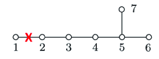
Figure 8: Dynkin Diagram of SO_2N illustrated for the example where $N=7$. By cutting the first node $\alpha_{1},$ one ends with the Diagram associated with the Dynkin diagram of the D_N-1 subalgebra and a free node $\alpha_{1}$ capturing data on the SO₂ Levi-charge and nilpotent subalgebras.

Denoting the basis vectors like $\left\{\left|+\right\rangle,\left|i\right\rangle,\left|-\right\rangle\right\}$ with label $i=1,...,2N-2,$ the Levi- constraint relations giving the generators $X_{i}$ and $Y^{i}$ of the nilpotent $\boldsymbol{n}_{\pm}$ are solved by

$$X_{i}$$

(3.40)

and

$$\mathbf{\mu}=\left|+\right\rangle\left\langle+\right|+q\sum_{i}\left|i\right\rangle\left\langle i\right|-\left|-\right\rangle\left\langle-\right|$$ (3.41)

where $q=0$, it has been inserted for convenience. The oscillator realisation of the Lax operator $\mathcal{L}_{D}^{vect}$ in the fundamental $2N$ representation is given by

$$\mathcal{L}_{D}^{\mu_{1}}=\left(\begin{array}[]{ccc}z+\mathbf{b^{T}.c+}\frac{1}{4}z^{-1}\mathbf{b}^{2}\mathbf{c}^{2}&\mathbf{b}^{T}-\frac{1}{2}z^{-1}\mathbf{b}^{2}\mathbf{c}^{T}&\frac{1}{2}z^{-1}\mathbf{b}^{2}\\ \mathbf{c-}\frac{1}{2}z^{-1}\mathbf{c}^{2}\mathbf{b}&I_{2N-2}+z^{-1}\mathbf{b^{T}.c}&-z^{-1}\mathbf{b}\\ \frac{1}{2}z^{-1}\mathbf{c}^{2}&-z^{-1}\mathbf{c}^{T}&z^{-1}\end{array}\right)$$ (3.42)

In this relation, we have $\mathbf{b}^{T}=\left(0,b_{1},...,b_{2N-2},0\right)$ and $\mathbf{c}^{T}=\left(0,c_{1},...,c_{2N-2},0\right)$ where the $(b^{i},c_{i})$ are harmonic oscillators associated with the phase space of the vector like $D_{N}$- system.

$\mathbf{II)}$ Spinorial coweight
In this case, the minuscule coweight is given by $\mu_{N}$. The Levi-decomposition is given by $so_{2}\oplus sl_{N}\oplus N\left(N-1\right)_{\pm},$ it results from cutting the N-th node $\alpha_{N}$ in the Dynkin diagram of D${}_{N}\simeq so_{2N}$ as in the Figure 9, 

Figure 9: Dynkin Diagram of SO_2N illustrated for the example where N=7. By cutting the node $\alpha_{N},$ one ends with the Diagram associated with the Levi subalgebra of A_N-1 and a free node $\alpha_{N}$.

The Wilson charge representation 2N decomposes in this case like $N_{+1/2}\oplus N_{-1/2}.$ Using the basis vectors $\left\{\left|i\right\rangle,\left|\bar{\imath}\right\rangle\right\}$ with label $1\leq i\leq N$ and label $\bar{\imath}=2N+1-i$ taking the values $\bar{1}\leq\bar{\imath}\leq\bar{N},$ we solve the Levi-constraint relations by

$$X_{i\bar{j}}$$

(3.43)

with

$$\mathbf{\mu}=\frac{1}{2}\sum_{i}\left|i\right\rangle\left\langle i\right|-\frac{1}{2}\sum_{\bar{\imath}}\left|\bar{\imath}\right\rangle\left\langle\bar{\imath}\right|$$ (3.44)

The calculation of the Lax matrix $\mathcal{L}_{D_{N}}^{\mu_{N}}=e^{X}z^{\mu}e^{Y}$ with $X=b^{i\bar{j}}X_{i\bar{j}}$ and $Y=c_{i\bar{j}}Y^{\bar{\imath}j}$ leads to

$$\mathcal{L}_{D_{N}}^{\mu_{N}}=\left(\begin{array}[]{cc}z^{\frac{1}{2}}+z^{-\frac{1}{2}}BC&z^{-\frac{1}{2}}B\\ z^{-\frac{1}{2}}C&z^{-\frac{1}{2}}\end{array}\right)$$ (3.45)

In this relation, the N$\times$N̄ matrix $B$ and the N̄$\times$N matrix $C$ are given by:

$$B=\left\{\begin{array}[]{ccc}b^{i\bar{j}}&&i<j\\ -b^{j\bar{\imath}}&&j<i\\ 0&&i=j\end{array}\right.,\qquad C=\left\{\begin{array}[]{ccc}c_{\bar{j}i}&&i<j\\ -c_{\bar{\imath}j}&&j<i\\ 0&&i=j\end{array}\right.$$ (3.46)

In matrix notations, we have

$$B=\left(\begin{array}[]{ccccc}b_{1\bar{N}}&b_{1\bar{N}-\bar{1}}&\cdots&b_{1\bar{2}}&0\\ b_{2\bar{N}}&b_{2\bar{N}-\bar{1}}&\cdots&0&-b_{1\bar{2}}\\ \vdots&\vdots&\ddots&\vdots&\vdots\\ b_{N-1,\bar{N}}&0&\cdots&-b_{2,\bar{N}-\bar{1}}&-b_{1,\bar{N}-\bar{1}}\\ 0&-b_{N-1,\bar{N}}&\cdots&-b_{2\bar{N}}&-b_{1\bar{N}}\end{array}\right)$$ (3.47)

and

$$C=\left(\begin{array}[]{ccccc}c_{\bar{N}1}&c_{\bar{N}2}&\cdots&c_{\bar{N},N-1}&0\\ c_{\bar{N}-\bar{1},1}&c_{\bar{N}-\bar{1},2}&\cdots&0&-c_{\bar{N}-\bar{1},N}\\ \vdots&\vdots&\ddots&\vdots&\vdots\\ c_{\bar{2}1}&0&\cdots&-c_{\bar{2},\bar{N}-\bar{1}}&-c_{\bar{2},N}\\ 0&-c_{\bar{1}2}&\cdots&-c_{\bar{1}N-1}&c_{\bar{1}N}\end{array}\right)$$ (3.48)

$\mathbf{III)}$ Cospinorial coweight
In this case, the minuscule coweight is given by $\mu_{N-1}$. The Levi-decomposition is given by $so_{2}\oplus sl_{N}^{\prime}\oplus N\left(N-1\right)_{\pm};$ it corresponds to cutting the node $\alpha_{N-1}$ in the Dynkin diagram of the Figure 10.

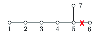
Figure 10: Dynkin Diagram of SO_2N illustrated for the example where N=7. By cutting the node $\alpha_{N-1},$ one ends with the Diagram associated with the Levi subalgebra of A’_N-1 and a free node $\alpha_{N-1}$.

Here, the $A_{N-1}^{\prime}\simeq sl_{N}^{\prime}$ is isomorphic to the $A_{N-1}\simeq sl_{N}$ appearing in the decomposition using the coweight $\mu_{N}$ considered above. In the present case, the $sl_{N}^{\prime}$ results from cutting the N-th node $\alpha_{N-1}$ in the Dynkin diagram of $so_{2N}$ while cutting the node $\alpha_{N}$ yields $sl_{N}$. As such, the simple root systems of the $sl_{N}^{\prime}$ and $sl_{N}$ are isometric and are given by

$$sl_{N}^{\prime}$$ :

:

(3.49)

These two systems are related to each other by the outer-automorphism symmetry $\mathbb{Z}_{2}$ acting by permutation of the simple roots $\alpha_{N-1}$ and $\alpha_{N}$ as follows

$$\mathbb{Z}_{2}:\left\{\begin{array}[]{lllll}\alpha_{i}&\rightarrow&\alpha_{i}&\text{ \ for \ }&1\leq i\leq N-2\\ \alpha_{N-1}&\rightarrow&\alpha_{N}&&\\ \alpha_{N}&\rightarrow&\alpha_{N-1}&&\end{array}\right.$$ (3.50)

Notice that the above $\mathbb{Z}_{2}$ discrete symmetry acts non trivially on the 2N quantum states $\left|a\right\rangle,$ with label $1\leq a\leq 2N,$ propagating along the Wilson line. As this electric line carries a vector-like charge given by the SO_2N representation; and by using the decomposition $2N=N_{+1/2}\oplus N_{-1/2}$ respectively labeled by $\left|i\right\rangle$ and $\left|\bar{\imath}\right\rangle$ with $1\leq i\leq N$ and $\bar{\imath}=2N+1-i$ taking the values $\bar{1}\leq\bar{\imath}\leq\bar{N},$ we end up with the following transformations

$$\mathbb{Z}_{2}:\left\{\begin{array}[]{lllll}\left|i\right\rangle&\rightarrow&\left|i\right\rangle&\text{ \ for \ }&1\leq i\leq N-2\\ \left|N-1\right\rangle&\rightarrow&\left|N\right\rangle&&\\ \left|N\right\rangle&\rightarrow&\left|N-1\right\rangle&&\end{array}\right.$$ (3.51)

Under this transformation, the charge operator (3.44) is preserved because the sums $\sum\left|i\right\rangle\left\langle i\right|$ and $\sum\left|\bar{\imath}\right\rangle\left\langle\bar{\imath}\right|$ are not affected by (3.51). The same invariance holds for the linear expansions $X=b^{i\bar{j}}X_{i\bar{j}}$ and $Y=c_{i\bar{j}}Y^{\bar{\imath}j}$. So, the Lax-matrix $\mathcal{L}_{D}^{\mu_{N-1}}$ is the same as $\mathcal{L}_{D}^{\mu_{N}}$ namely

$$\mathcal{L}_{D}^{\mu_{N-1}}=\left(\begin{array}[]{cc}z^{\frac{1}{2}}+z^{-\frac{1}{2}}BC&z^{-\frac{1}{2}}B\\ z^{-\frac{1}{2}}C&z^{-\frac{1}{2}}\end{array}\right)$$ (3.52)

3.3.5 Exceptional Lax operators

As there is no minuscule coweight in the exceptional Lie algebra E₈, we have minuscule Lax-operators only for the 4D exceptional Chern-Simons with gauge symmetries E₆ and E₇. From the classification Table 1, we learn that $\left(\mathbf{i}\right)$ the E₆ gauge model has two minuscule L-operators $\mathcal{L}_{E_{6}}^{\mu_{1}}$ and $\mathcal{L}_{E_{6}}^{\mu_{5}}.$ $\left(\mathbf{ii}\right)$ the E₇ gauge model has one minuscule $\mathcal{L}_{E_{7}}^{\mu_{1}}$. They are described here below.

$\mathbf{I)}$ Lax-matrices $\mathcal{L}_{E_{6}}^{\mu_{1}}$ and $\mathcal{L}_{E_{6}}^{\mu_{5}}$:
The Lax operator of E₆-type for the coweight $\mu_{1}$ is associated with the Levi-decomposition $E_{6}\rightarrow so_{10}\oplus so_{2}\oplus 16_{+}\oplus 16_{-}$. In the diagrammatic language, this corresponds to omitting the first node in the Dynkin diagram of $E_{6}$ given by the Figure 11.

Figure 11: Dynkin Diagram of E₆ having six nodes labeled by the six simple roots $\alpha_{i}$. The cross $\left(\times\right)$ indicates the roots used in the Levi decomposition with Levi subalgebra as $so_{10}\oplus so_{2}.$

This node, labeled by simple root $\alpha_{1},$ corresponds to the fundamental $\mathbf{27}$ representation of E₆ with quantum states $\left|\varphi\right\rangle$ propagating along the Wilson line. These 27 quantum states decompose with respect to the Levi-subalgebra as follows

$$27=1_{-4/3}\oplus 10_{+2/3}\oplus 16_{-1/3}$$ (3.53)

So, we split the 27 states of the representation $\mathbf{27}$ like: $\left(i\right)$ a state $\left|0\right\rangle$ denoting the singlet $1_{-4/3}$; $\left(ii\right)$ ten states $\left\{\left|i\right\rangle\right\}_{1\leq i\leq 10}$ designating the ten-uplet $10_{+2/3}$ and $\left(iii\right)$ sixteen states $\left\{\left|\beta\right\rangle\right\}_{1\leq\beta\leq 16}$ representing the $16_{-1/3}$. Using these states, we solve the Levi-constraint relations for generators of the nilpotent subalgebras $\mathbf{16}_{\pm}$ as

$$X_{\beta}$$

(3.54)

and

$$\mathbf{\mu}=-\frac{4}{3}\left|0\right\rangle\left\langle 0\right|+\frac{2}{3}\sum_{i}\left|i\right\rangle\left\langle i\right|-\frac{1}{3}\sum_{\beta}\left|\beta\right\rangle\left\langle\beta\right|$$ (3.55)

where $\Gamma^{i}$ are $so_{10}$ Dirac-like matrices satisfying the euclidian Clifford algebra. Putting these relations back into $\mathcal{L}_{E_{6}}^{\mu_{1}}=e^{X}z^{\mu}e^{Y}$, we obtain after tedious but straightforward algebra the following expression,

$$\mathcal{L}_{E_{6}}^{\mu_{1}}=\left(\begin{array}[]{ccc}z^{-\frac{4}{3}}&z^{-\frac{4}{3}}W_{j}&z^{-\frac{4}{3}}c_{\beta}\\ z^{-\frac{4}{3}}V^{i}&z^{\frac{2}{3}}\delta_{j}^{i}+z^{-\frac{4}{3}}V^{i}W_{j}+z^{-\frac{1}{3}}B_{\alpha}^{i}C_{j}^{\alpha}&z^{-\frac{4}{3}}V^{i}c_{\beta}+z^{-\frac{1}{3}}B_{\beta}^{i}\\ z^{-\frac{4}{3}}b^{\alpha}&z^{-\frac{4}{3}}b^{\alpha}W_{j}+z^{-\frac{1}{3}}C_{j}^{\alpha}&z^{-\frac{1}{3}}\delta_{\beta}^{\alpha}+z^{-\frac{4}{3}}b^{\alpha}c_{\beta}\end{array}\right)$$ (3.56)

where we have defined the following quantities in terms of the oscillator degrees of freedom $b^{\alpha}$ and $c_{\beta}.$

$$B_{\beta}^{i}=b^{\gamma}\Gamma_{\gamma\beta}^{i}$$ ,

,

(3.57)

The Lax operator $\mathcal{L}_{E_{6}}^{\mu_{5}}$ associated to the coweight $\mu_{5}$ is obtained in a similar way as before; but instead of cutting the first node $\alpha_{1}$ in the Dynkin diagram of E₆, we need to cut the fifth $\alpha_{5}$. Because this node corresponds to the anti-fundamental representation $\overline{\mathbf{27}},$ it is realised in the same basis as in (3.54-3.55) but with $\mathbf{\mu}$ replaced with the opposite $-\mathbf{\mu}$. This feature leads to the relationship

$$\mathcal{L}_{E_{6}}^{\mu_{5}}\left(z\right)=\mathcal{L}_{E_{6}}^{\mu_{1}}\left(1/z\right)$$ (3.58)

The properties of the exceptional Lax operators $\mathcal{L}_{E_{6}}^{\mu}$ were briefly outlined in [25] and its detailed derivation can be found in [34].

$\mathbf{II)}$ Lax-matrix $\mathcal{L}_{E_{7}}$
The gauge symmetry group $E_{7}$ of the 4D Chern-Simons theory is characterized by one minuscule coweight $\mu_{1}$ corresponding to the fundamental representation $\mathbf{56}$. As shown on the Tables 1-2, the Levi-subalgebra of $E_{7}$ contains its subalgebra E₆ and the nilpotent $\boldsymbol{n}_{\pm}$ are given by $\mathbf{27}_{\pm}$. This corresponds to cutting the node $\alpha_{6}$ as depicted by the Figure 3.62.

Figure 12: Dynkin Diagram of E₇ having seven nodes labeled by the simple roots $\alpha_{i}$. The cross $\left(\times\right)$ indicates the roots used in the Levi decomposition with Levi subgroup $SO(2)\times E_{6}.$

The quantum states $\left|a\right\rangle$ running on the electrically charged Wilson line are described by the representation $\mathbf{56}$ that decomposes as follows

$$\mathbf{56=1}_{3/2}\oplus\mathbf{27}_{1/2}\oplus\overline{27}_{-1/2}\oplus\mathbf{\bar{1}}_{-3/2}$$ (3.59)

As such, the 56 states $\left|a\right\rangle$ can be splitted as $\left|0_{+}\right\rangle,\left|\beta_{+}\right\rangle,\left|\beta_{-}\right\rangle,\left|0_{-}\right\rangle$ where the labels take the values $\beta_{+}=1,...,27$ and $\beta_{-}=\bar{1},...,\overline{27}.$ The generators of $\boldsymbol{n}_{\pm}$ solving the Levi-conditions are given by

$$X_{\beta}$$

(3.60)

such that the $\Gamma_{\beta}^{\delta_{+}\gamma_{-}}$ and $\bar{\Gamma}_{\gamma_{-}\delta_{+}}^{\beta}$ are tri-coupling objects of the E₆ representation theory [34]. The Levi- charge operator is given by

$$\mathbf{\mu}=\frac{3}{2}\left|0_{+}\right\rangle\left\langle 0_{+}\right|+\frac{1}{2}\sum_{\beta_{+}}\left|\beta_{+}\right\rangle\left\langle\beta_{+}\right|-\frac{1}{2}\sum_{\beta_{-}}\left|\beta_{-}\right\rangle\left\langle\beta_{-}\right|-\frac{3}{2}\left|0_{-}\right\rangle\left\langle 0_{-}\right|$$ (3.61)

The derivation of the Lax-matrix $\mathcal{L}_{E_{7}}^{\mu_{1}}$ is a little bit technical and cumbersome, we choose to represent it in the basis $\left|0_{+}\right\rangle,\left|\beta_{+}\right\rangle,\left|\beta_{-}\right\rangle,\left|0_{-}\right\rangle$ as follows

$$\mathcal{L}_{E_{7}}^{\mu_{1}}=\left(\begin{array}[]{cccc}L_{0_{+}}^{0_{+}}&L_{0_{+}}^{\beta_{+}}&L_{0_{+}}^{\beta_{-}}&L_{0_{+}}^{0-}\\ L_{\alpha_{+}}^{0_{+}}&L_{\alpha_{+}}^{\beta_{+}}&L_{\alpha_{+}}^{\beta_{-}}&L_{\alpha_{+}}^{0-}\\ L_{\alpha_{-}}^{0_{+}}&L_{\alpha_{-}}^{\beta_{+}}&L_{\alpha_{-}}^{\beta_{-}}&L_{\alpha_{-}}^{0-}\\ L_{0-}^{0_{+}}&L_{0-}^{\beta_{+}}&L_{0-}^{\beta_{-}}&L_{0-}^{0-}\end{array}\right)$$ (3.62)

The diagonal entries of this Lax-matrix are given by

$$L_{0_{+}}^{0_{+}}$$

(3.63)

with $\mathcal{E}=b^{\alpha}b^{\beta}b^{\beta}\Gamma_{\alpha\beta\gamma}$ and $\mathcal{F}=\bar{\Gamma}^{\alpha\beta\gamma}c_{\alpha}c_{\beta}c_{\gamma}$. The other Lax-matrix entries are as listed below

$${\small L}_{{\small 0}_{+}}^{{\small\beta}_{+}}$$

(3.64)

and

$$L_{\alpha_{-}}^{0_{+}}$$

(3.65)

as well as

$$L_{0_{+}}^{0-}$$ ,

,

,

(3.66)

More details concerning the derivation of this operator from the 4D Chern- Simons theory can be found in [34].

4 B-type Lax operators

In this section, we calculate the minuscule Lax operator $\mathcal{L}_{B}(z)$ from the 4D Chern- Simons theory with gauge symmetry $SO_{2N+1}.$ The $\mathcal{L}_{B}^{\mu}$ is determined by using the formula $e^{X}z^{\mu}e^{Y}$. In this relation, the $\mu$ is the minuscule coweight of the underlying Lie algebra $B_{N}$ of the gauge symmetry. The $X=b^{i}X_{i}$ and $Y=c_{i}X^{i}$ are $\left(2N+1\right)\times\left(2N+1\right)$ matrices valued in the nilpotent algebras $\boldsymbol{n}_{-}$ and $\boldsymbol{n}_{+}$ appearing in the Levi-decomposition of $B_{N}\sim so_{2N+1}$ with respect to $\mu,$ namely

$$so_{2N+1}$$

       

(4.1)

Dimensions and ranks of the algebras appearing in (4.1) can be directly read from the following decompositions

$$\dim$$ :

:

(4.2)

Recall that the finite dimensional Lie algebra $B_{N}$ has one minuscule coweight $\mu_{1}=e_{1}$ (denoted here as $\mu$); it is the dual of the simple root $\alpha_{1}=e_{1}-e_{2}$ ($\mu_{1}.\alpha_{i}=\delta_{1i}$); and corresponds to the first node of the Dynkin diagram of $B_{N}$. For an illustration, see the Figure 6.
The nilpotent sub-algebras are generated by X_i and Yⁱ obeying the following commutation relations

$$\left[\mathbf{\mu},X_{i}\right]$$

(4.3)

where $\mathbf{\mu}$ stands for the adjoint action of the minuscule coweight. The explicit realisation of this algebra in terms of the harmonic oscillators of the phase space of the L-operators is investigated below.

4.1 Solving Levi-constraint relations

To solve (4.3), we need to define the Levi-decomposition of the vectorial representation $\mathbf{2N+1}$ of the Lie algebra $so_{2N+1}$ and related objects. Vector states of $\mathbf{2N+1}$ propagate on the Wilson line interacting with the ’t Hooft line with magnetic charge $\mu$. Under the Levi-decomposition, the real $\mathbf{2N+1}$ representation of so_2N+1 splits as direct sum of representations of $\boldsymbol{l}_{\mu}=so_{2}\oplus so_{2N-1}$. In fact, we have $\mathbf{2N+1}=\mathbf{2_{0}\oplus(2N-1)_{0}}$ where the zero label refers to the charge under the group $SO\left(2\right)\mathbf{.}$ By using the isomorphism $SO\left(2\right)\sim U(1),$ we can put this decomposition to the following form

$$\mathbf{2N+1}=\mathbf{1}_{+1}\oplus\left(\mathbf{2N-1}\right)_{0}\oplus\mathbf{1}_{-1}$$ (4.4a)

where we have substituted with $$\mathbf{2_{0}}=\mathbf{1}_{+1}\oplus\mathbf{1}_{-1} \left(\left|+\right\rangle,\left|i\right\rangle,\left|-\right\rangle\right) i=1,...,2N-1 \left(\left\langle+\right|,\left\langle i\right|,\left\langle-\right|\right) (\mathbf{2N+1)}$$. For convenience, we use the kets with and the bras to denote the vector basis of the fundamental representation and its dual. We have

$$\left|\mathbf{2N+1}\right\rangle=\left(\begin{array}[]{c}\left|+\right\rangle\\ \left|\mathbf{2N-1}\right\rangle\\ \left|-\right\rangle\end{array}\right)$$ (4.5)

where $\left|\pm\right\rangle$ refer to the two complex singlets $\mathbf{1}_{\pm 1}$ in the decomposition (4.4a) and $\left|\mathbf{2N-1}\right\rangle$ represents the $2N-1$ states $\left\{\left|i\right\rangle\right\}_{1\leq i\leq 2N-1}.$ This basis is characterized by the following orthogonality relations $\left\langle+|-\right\rangle=\left\langle+|i\right\rangle=\left\langle i|-\right\rangle=0$ and $\left\langle+|+\right\rangle=\left\langle-|-\right\rangle=1,$ as well as $\left\langle i|j\right\rangle=\delta_{ij}.$
The next step is to find the adjoint action $\mathbf{\mu}$ of the minuscule coweight on the fundamental representation. This is a hermitian charge operator acting on the quantum states generated by (4.5). It can be represented like

$$\mathbf{\mu}=\varrho_{+}+q\Pi-\varrho_{\mathbf{-}}$$ (4.6)

where $\varrho_{\pm}$ are the projectors on the representation sub-spaces $\mathbf{1}_{\pm 1}$ appearing in (4.4a) and $\Pi$ is the projector on $\left(\mathbf{2N-1}\right)_{0}$. These projectors read in terms of the bras/kets as follows

$$\varrho_{+}$$

(4.7)

and

$$\Pi=\sum_{i=1}^{2N-1}\varrho_{i}$$ (4.8)

Notice here that the charge $q$ vanishes ($q=0)$ because the $\left|\mathbf{2N-1}\right\rangle$ is chargeless. Now, we move to working out the explicit expressions of the generators $X_{i}$ and $Y^{i}$ of the nilpotent algebras $\boldsymbol{n}_{+}$ and $\boldsymbol{n}_{-}$ in the basis 4.5. They are obtained by solving the Levi-constraint relations (4.3). By taking $X_{i}$ and $Y^{i}$ like

$$X_{i}$$

(4.9)

with $x_{1,2}$ and $y_{1,2}$ non vanishing arbitrary numbers, then using $\mathbf{\mu}=\varrho_{+}-\varrho_{\mathbf{-}},$ we have $\left[\mathbf{\mu},X_{i}\right]=+X_{i}$ and $\left[\mathbf{\mu},Y^{i}\right]=-Y^{i}$ as well as $\left[X_{i},Y^{i}\right]=\delta_{i}^{i}\mathbf{\mu}$ provided the following conditions are satisfied: $\left(\mathbf{i}\right)$ $x_{2}y_{2}=x_{1}y_{1}$ and $\left(\mathbf{ii}\right)$ $x_{1}y_{1}=x_{2}y_{2}=1.$ These conditions can be solved by taking

$$x_{1}y_{1}=1\qquad,\qquad x_{2}=y_{2}=\pm 1$$ (4.10)

Below, we take $x_{2}=y_{2}=-1$. With these generators, we can express the $X$ and $Y$ matrices appearing in the Lax operator that we want to calculate; we have

$$X=b^{i}X_{i}\in n_{+}\qquad,\qquad Y=c_{i}Y^{i}\in n_{-}$$ (4.11)

In these expansions, the $b^{i}$ and the $c_{i}$ variables are the phase space coordinates of the $\mathcal{L}_{B}$-operator; they are treated here classically but they can be promoted to operators without ambiguity. This is because in the formula $e^{X}z^{\mu}e^{Y},$ the $b^{i}$’s are in the left and the $c_{i}$’s are in the right in agreement with the Wick theorem.

4.2 Building the operator $\mathcal{L}_{B}$

We begin by calculating the exponentials $e^{X}$ and $e^{Y}$ by using the expansion $e^{A}=\sum A^{n}/n!.$ Based on the eqs (4.9), we compute the powers of the $X_{i}$ and $Y^{i}$ generators. We find after some calculations that

$$X_{i}X_{j}$$

(4.12)

and

$$X_{i}X_{j}X_{k}$$

(4.13)

From these relations and the expansions $X=b^{i}X_{i}$ and $Y=c_{i}Y^{i}$, we deduce that $X{{}^{2}}=\mathbf{b}^{2}\left|+\right\rangle\left\langle-\right|$ with $\mathbf{b}^{2}=b^{i}\delta_{ij}b^{j}$ and $Y{{}^{2}}=\mathbf{c}^{2}\left|-\right\rangle\left\langle+\right|$ with $\mathbf{c}^{2}=c_{i}\delta^{ij}c_{j}$. We also have $e^{X}=1+X+X^{2}/2$ and $e^{Y}=1+Y+Y^{2}/2$ because $X^{3}=Y^{3}=0.$ These features lead to the following polynomial-like expansion

$$\mathcal{L}_{B}=\left(1+X+\frac{1}{2}X^{2}\right)z^{\mathbf{\mu}}\left(1+Y+\frac{1}{2}Y^{2}\right)$$ (4.14)

reading explicitly as

$$\mathcal{L}_{B}$$

(4.15)

Replacing $z^{\mathbf{\mu}}$ with

$$z^{\mathbf{\mu}}=z\varrho_{+}+\Pi+z^{-1}\varrho_{-}$$ (4.16)

and taking advantage of the properties $X_{i}\varrho_{+}=0$ and $\varrho_{+}Y^{i}=0$ as well as

$$X\varrho_{+}$$

(4.17)

we obtain

$$\mathcal{L}_{B}$$

(4.18)

To determine the matrix representation of the L-operator, we use the following trick (projector basis)

$$\mathcal{L}_{B}=\left(\begin{array}[]{ccc}\varrho_{+}L\varrho_{+}&\varrho_{+}L\Pi&\varrho_{+}L\varrho_{-}\\ \Pi L\varrho_{+}&\Pi L\Pi&\Pi L\varrho_{-}\\ \varrho_{-}L\varrho_{+}&\varrho_{-}L\Pi&\varrho_{-}L\varrho_{-}\end{array}\right)$$ (4.19)

By substituting $X=b^{i}X_{i}$ and $Y=c_{i}Y^{i}$, we end up with the following result

$$\mathcal{L}_{B}^{\mu_{1}}=\left(\begin{array}[]{ccc}z+\mathbf{b}^{T}\mathbf{.c}+\frac{1}{4}z^{-1}\mathbf{b}^{2}\mathbf{c}^{2}&\mathbf{b}^{T}-\frac{1}{2}z^{-1}\mathbf{b}^{2}\mathbf{c}^{T}&\frac{1}{2}z^{-1}\mathbf{b}^{2}\\ \mathbf{c}-\frac{1}{2}z^{-1}\mathbf{c}^{2}\mathbf{b}&I_{2N-1}+z^{-1}\mathbf{b}^{T}\mathbf{.c}&-z^{-1}\mathbf{b}\\ \frac{1}{2}z^{-1}\mathbf{c}^{2}&-z^{-1}\mathbf{c}^{T}&z^{-1}\end{array}\right)$$ (4.20)

where $\mathbf{f}^{T}$ stands for the row vector ($f_{1},...,f_{2N-1}$). Notice the two following features regarding eq(4.20).
$\left(\mathbf{1}\right)$ By multiplication of $\mathcal{L}_{B}^{\mu_{1}}$ by z, we recover the Lax-matrix of B-type obtained in [33] by using anti-dominant shifted Yangians.
$\left(\mathbf{2}\right)$ Eq(4.20 has a quite similar form to the Lax operator $\mathcal{L}_{D}^{{\small vec}}$ of the $SO_{2N}$ family given by eq(3.42). The main difference concerns the number of $\left(b,c\right)$ oscillators that appears in the middle block. For $\mathcal{L}_{D_{N+1}}^{{\small vec}}$, we have $2N$ oscillators versus $2N-1$ oscillators for $\mathcal{L}_{B_{N}}.$ This property can be explained by the fact that the B_N Dynkin diagram can be obtained from the folding the two spinorial-like nodes of the D_N+1 Dynkin diagram as depicted by the Figure 13. In this folding, the vectorial minuscule coweight is preserved. 

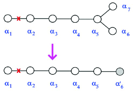
Figure 13: Folding the nodes $\alpha_{N-1}$ and $\alpha_{N}$ of the Dynkin Diagram of D_N+1 giving the Dynkin diagram of B_N. This folding commutes with the cutting of the node $\alpha_{1}$.

5 C-type Lax operators

In this section, we derive the minuscule Lax operator $\mathcal{L}_{C}(z)$ from the 4D Chern- Simons theory with gauge symmetry $SP_{2N}.$ The $\mathcal{L}_{C}^{\mu}$ is determined by using the formula $e^{X}z^{\mu}e^{Y}$. Here, the $\mu$ is the minuscule coweight of the Lie algebra $C_{N}\sim sp_{2N}$ and the $X$ and $Y$ are $2N\times 2N$ matrices belonging to the nilpotent sub-algebras $\boldsymbol{n}_{-}$ and $\boldsymbol{n}_{+}$ appearing in the Levi-decomposition of $sp_{2N},$ namely

$$sp_{2N}$$

(5.1)

The dimensions and the ranks of the algebras involved in this decomposition are as given below

$$\dim$$ :

:

(5.2)

Recall that the Lie algebra $C_{N}$ has one minuscule coweight reading in terms of the $\left\{e_{i}\right\}$ weight vector basis as $\mu=\mu_{N}=\frac{1}{2}\left(e_{1}+...+e_{N}\right)$. This minuscule coweight is the dual of the simple root $\alpha_{N}=2e_{N}$, it corresponds to the N-th node of the Dynkin diagram of $C_{N}$ given by the Figure 7.
Recall also that in (5.1), $\boldsymbol{l}_{\mu}$ is the Levi-subalgebra of $sp_{2N}$ and the $\boldsymbol{n}_{\pm}$ are the nilpotent sub-algebras having $\frac{1}{2}N\left(N+1\right)$ dimensions that split like $\frac{1}{2}N\left(N-1\right)+N$. These subalgebras are generated by matrix generators denoted like $\left(X_{\left[i\bar{j}\right]},X_{i\bar{\imath}}\right)$ and $\left(Y^{\left[\bar{\imath}j\right]},Y^{\bar{\imath}i}\right).$ They obey the following commutation relations

$$\left[\mathbf{\mu},X_{i\bar{\imath}}\right]$$

(5.3)

where $\mathbf{\mu}$ stands for the adjoint action of the minuscule coweight.

5.1 Solving Levi-constraints for C_N

To solve the constraint relations (5.3), we need the Levi-decomposition of the fundamental representation $\mathbf{2N}$ of the Lie algebra $sp_{2N}$ given by

$$\mathbf{2N}=\mathbf{N}_{+1/2}\oplus\mathbf{N}_{-1/2}\equiv\mathbf{N}\oplus\mathbf{\bar{N}}$$ (5.4a)

where $$\mathbf{N}_{+1/2} \mathbf{N}_{-1/2} \pm 1/2 \left(\mathbf{a}\right) \left\{\left|i\right\rangle,\left|\bar{\imath}\right\rangle\right\} i=1,...,N \bar{\imath}=2N+1-i \mathbf{2N} \bar{\imath} \bar{\imath}=\bar{N},...,\bar{1} \left(\mathbf{b}\right) \left\{\left\langle i\right|,\left\langle\bar{\imath}\right|\right\} \mathbf{2N}$$ and are representations of sl_N and the subscripts referring to the SO₂ charges. To proceed, we use the 2N kets with and to represent the quantum basis states of the symplectic representation . For convenience, we order the -label like . the dual bras to denote the vector basis of ()^T. Formally, we have

$$\left|\mathbf{2N}\right\rangle=\left(\begin{array}[]{c}\left|i\right\rangle\\ \left|\bar{\imath}\right\rangle\end{array}\right)\qquad,\qquad\left\langle\mathbf{2N}\right|=\left(\begin{array}[]{c}\left\langle i\right|\\ \left\langle\bar{\imath}\right|\end{array}\right)$$ (5.5)

The next step is to work out the adjoint action $\mathbf{\mu}$ of the minuscule coweight on the fundamental representation $\mathbf{2N}$. It is given by

$$\mathbf{\mu}=\frac{1}{2}\Pi_{{}_{\mathbf{N}}}-\frac{1}{2}\Pi_{{}_{\mathbf{\bar{N}}}}$$ (5.6)

with the projectors on $\mathbf{N}_{+1/2}$ and $\mathbf{N}_{-1/2}$ as follows

$$\Pi_{{}_{\mathbf{N}}}=\sum_{i=1}^{N}\varrho_{i}\qquad,\qquad\Pi_{{}_{\mathbf{\bar{N}}}}=\sum_{\bar{\imath}=\bar{1}}^{\bar{N}}\bar{\varrho}_{i}$$

In these relations, we have set

$$\varrho_{i}$$

(5.7)

Now, we move to the determination of explicit expressions of the matrices $\left(X_{\left[i\bar{j}\right]},X_{i\bar{\imath}}\right)$ and $\left(Y^{\left[\bar{\imath}j\right]},Y^{\bar{\imath}i}\right)$ generating the nilpotent algebras $\boldsymbol{n}_{+}$ and $\boldsymbol{n}_{-}$. They are obtained by solving the Levi-constraint relations (5.3), we have found

$$X_{i\bar{\imath}}$$

(5.8)

and

$$Y^{\bar{\imath}i}$$

(5.9)

They also obey other useful properties such as $[X_{i\bar{\imath}},X_{\left[k\bar{l}\right]}]=0$ and $\left[Y^{\bar{\imath}i},Y^{\left[\bar{k}l\right]}\right]=0.$ With the generators (5.8-5.9), we can express the X and Y matrices appearing in the Lax operator. We have

$$X$$

(5.10)

In these expansions, the $\left\{b^{i\bar{\imath}},b^{\left[i\bar{j}\right]}\right\}$ and the $\left\{c_{\bar{\imath}i},c_{\left[\bar{\imath}j\right]}\right\}$ variables are the phase space coordinates of the $\mathcal{L}_{C}$-operator.

5.2 Building the operator $\mathcal{L}_{C}$

First, we use eqs(5.8-5.9) to determine the powers $X$ and $Y.$ Then, we calculate the exponentials $e^{X}$ and $e^{Y}$ appearing in the L-operator formula. Straightforward algebra leads to

$$X_{i\bar{\imath}}X_{j\bar{j}}$$     ,

    ,

    ,

(5.11)

These properties show that the exponentials take simple forms $e^{X}=I_{2N}+X$ and $e^{Y}=I_{2N}+Y.$ Then, the Lax operator expands as follows

$$\mathcal{L}_{C}=\left(1+X\right)z^{\mathbf{\mu}}\left(1+Y\right)$$ (5.12)

reading explicitly as

$$\mathcal{L}_{C}=z^{\mathbf{\mu}}+z^{\mathbf{\mu}}Y+Xz^{\mathbf{\mu}}+Xz^{\mathbf{\mu}}Y$$ (5.13)

Replacing the charge operator $z^{\mathbf{\mu}}$ with

$$z^{\mathbf{\mu}}=z^{\frac{1}{2}}\Pi+z^{-\frac{1}{2}}\bar{\Pi}$$ (5.14)

we get the following expression of the Lax operator for the symplectic family

$$\mathcal{L}_{C}$$

(5.15)

This relation can be simplified by taking advantage of properties of the X and Y matrices that descend from the generators realising (5.3). We have $X\Pi=0$ and $\Pi Y=0$ as well $X\bar{\Pi}=X$ and $\bar{\Pi}Y=Y.$ By substituting, we end up with

$$\mathcal{L}_{C}$$

(5.16)

In the projector basis $\left(\Pi,\bar{\Pi}\right)$, we have the following representation

$$\mathcal{L}_{C}=\left(\begin{array}[]{cc}z^{\frac{1}{2}}\Pi+z^{-\frac{1}{2}}\Pi XY\Pi&z^{-\frac{1}{2}}\Pi X\bar{\Pi}\\ z^{-\frac{1}{2}}\bar{\Pi}Y\Pi&z^{-\frac{1}{2}}\bar{\Pi}\end{array}\right)$$ (5.17)

which also reads as

$$\mathcal{L}_{C}=\left(\begin{array}[]{cc}z^{\frac{1}{2}}I_{N}+z^{-\frac{1}{2}}XY&z^{-\frac{1}{2}}X\\ z^{-\frac{1}{2}}Y&z^{-\frac{1}{2}}I_{N}\end{array}\right)$$ (5.18)

In the vector basis $\left\{\left|i\right\rangle,\left|\bar{\imath}\right\rangle\right\},$ we have

$$X=\left(\begin{array}[]{ccc}b^{1\bar{1}}&\cdots&b^{1\bar{N}}\\ \vdots&\ddots&\vdots\\ b^{N\bar{1}}&\cdots&b^{N\bar{N}}\end{array}\right),\qquad Y=\left(\begin{array}[]{ccc}c_{\bar{1}1}&\cdots&c_{\bar{1}N}\\ \vdots&\ddots&\vdots\\ c_{\bar{N}1}&\cdots&c_{\bar{N}N}\end{array}\right)$$ (5.19)

and

$$XY=\left(\begin{array}[]{ccc}b^{1\bar{\imath}}c_{\bar{\imath}1}&\cdots&b^{1\bar{\imath}}c_{\bar{\imath}N}\\ \vdots&\ddots&\vdots\\ b^{N\bar{\imath}}c_{\bar{\imath}1}&\cdots&b^{N\bar{\imath}}c_{\bar{\imath}N}\end{array}\right)$$ (5.20)

Finally, notice the two following features regarding (5.18):
$\left(\mathbf{1}\right)$ Eq(5.18) is, up to multiplication by z, similar to the Lax-matrix of C-type obtained in [33] by using anti-dominant shifted Yangians.
$\left(\mathbf{2}\right)$ The obtained relations (5.18-5.20) have a quite similar structure as the Lax operator $\mathcal{L}_{A_{2N}}^{\mu_{N}}$ of the $SL_{2N}$ family decomposed with respect to the fundamental coweight $\mu_{N}$ of $SL_{2N}$. This similarity feature between $\mathcal{L}_{C_{N}}^{\mu_{N}}$ and $\mathcal{L}_{A_{2N}}^{\mu_{N}}$ can be explained by the fact that the SP_2N Dynkin diagram is related to the $SL_{2N}$ Dynkin diagram by folding the nodes $\alpha_{i}$ and $\alpha_{2N-1-i}$ as shown on the Figure 14.

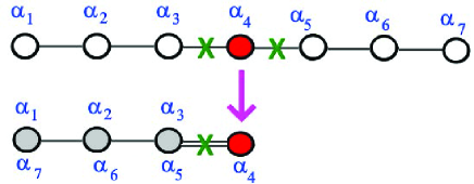
Figure 14: Folding the nodes $\alpha_{2M-1-i}$ and $\alpha_{i}$ of the Dynkin Diagram of A_2M-1 giving the Dynkin diagram of C_M. This folding commutes with the cutting of the node $\alpha_{M}$. The green cross ($\times$) refers to the cutting of the node $\alpha_{M}$. The folding is illustrated for the example M=4.

6 Conclusion and comments

Four dimensional Chern-Simons gauge theory proposed in [1] has been shown to be a powerful QFT approach to deal with lower dimensional integrable systems. Several results on integrable 1D quantum spin chains such as the Lax operators of A- and D-types, obtained by using Bethe Ansatz formalism and standard statistical physics as well as algebraic methods, were nicely derived from the CS theory. The investigation given in this paper is a contribution to the topological 4D CS gauge theory and its applications. It essentially aims to complete some partial results obtained in literature and also to gather the explicit expressions of minuscule Lax operators $\mathcal{L}_{G}$ and classify them according to algebraic properties of the gauge symmetry as given in the Tables 1-2 and the Table  3 given below. We recall that from the view point of the 4D Chern-Simons theory, the $\mathcal{L}_{G}$’s can be thought of as a matrix coupling an electrically charged Wilson line W${}_{\xi_{z}}^{\boldsymbol{R}}$ crossing a magnetically charged ’t Hooft line tH${}_{\xi_{0}}^{\boldsymbol{\mu}}$. The study of this crossing yields a general formula that corresponds to the oscillator realisation of the Lax operator for an integrable XXX spin chain. This construction was introduced in this paper along with the mathematical tools needed to build our results. Among our contributions, we quote the three following:
$\left(\mathbf{1}\right)$ We derived the non simply laced orthogonal B_N- and the symplectic C_N- families of Lax operators using the 4D CS theory method. These calculations have not been addressed before in the framework of the CS gauge theory. The Lax operators $\mathcal{L}_{B_{N}}$ and $\mathcal{L}_{C_{N}}$ were calculated in section 3 with regards the unified picture of all the $\mathcal{L}_{G}$’s. They were investigated with further details in sections 4 and 5 and they were shown to agree with recent expressions derived in the spin chain literature for the B_N and C_N symmetries.
$\left(\mathbf{2}\right)$ We gave an interpretation of the links between the B_N- and C_N-type Lax operators and their A_N- and D_N- homologue in terms of discrete symmetries and foldings with respect to discrete groups. We showed that these symmetries are nothing but the outer-automorphisms of Dynkin diagrams of A_N and D_N. These foldings were visualized in the Figures 13 and 14 showing the relationships between the B_N/C_N-types and D_N/A_N types.
$\left(\mathbf{3}\right)$ We built the set of the minuscule Lax operators labeled by a set parameters. In addition to the electric charge $\boldsymbol{R}$ of the Wilson line W${}_{\xi_{z}}^{\boldsymbol{R}}$, these parameters are given by the rank of the Lie algebra of the gauge symmetry G and its minuscule coweights $\mu$. The content of this set is given by the table 2. This basic set contains five subsets: four infinite given by the families A_N, B_N, C_N, D_N and one finite given by the exceptional E₆ and E₇ symmetries.
We end this paper by giving brief comments concerning the L-operators of the SO_2N symmetry having a spinorial $\boldsymbol{R}$ representation with dimension $\boldsymbol{R}=2^{N}$, this corresponds to having a Wilson line W${}_{\xi_{z}}^{2^{N}}$ in the spinor representation crossing a ’t Hooft line. The construction of the associated L-operator $\left.\mathcal{L}_{D_{N}}^{\mu}\right|_{{\small R=2}^{{\small N}}}$ can be done by following the same analysis that we performed in the sub-subsection 3.3.4 to build $\left.\mathcal{L}_{D_{N}}^{\mu}\right|_{{\small R=2}N}$. In fact, both the fundamental $\left.\mathcal{L}_{D_{N}}^{\mu}\right|_{{\small 2}^{{\small N}}}$ and $\left.\mathcal{L}_{D_{N}}^{\mu}\right|_{{\small 2}N}$ are calculated by using the following formulas

$$\left.\mathcal{L}_{D_{N}}^{\mu}\right|_{{\small R=2}^{{\small N}}} = \left.e^{X}z^{\mathbf{\mu}}e^{Y}\right|_{{\small R=2}^{{\small N}}}\qquad:Spin=2^{N}$$ (6.1)

$$\left.\mathcal{L}_{D_{N}}^{\mu}\right|_{{\small R=2}N} = \left.e^{X}z^{\mathbf{\mu}}e^{Y}\right|_{{\small R=2}N}\text{ \ }\qquad:Vect=2N$$ (6.2)

However, though they look quite similar, the expressions of these two operators are completely different, the first (6.1) is realised by a $\nu\times\nu$ matrix with $\nu=2^{N}$, while the second (6.2) is given by a $2N\times 2N$ matrix. So, the matrix realisations of the triplets $\left(\mathbf{\mu,}X,Y\right)$ used in (6.1) and in (6.2) are different. Below, we comment the matrix realisations of the triplet ($\mathbf{\mu}$,X,Y) involved in (6.1).
The Levi-charge $\mathbf{\mu}$ needed for the calculation of (6.1) is obtained by decomposing the $2^{N}$ representation as a direct sum of representations of the Levi -subalgebra $\boldsymbol{l}_{\mu}$ as in eqs(3.1-3.4). Because we have two types of $\boldsymbol{l}_{\mu}$’s namely $\left(\mathbf{i}\right)$ $so_{2}\oplus D_{N-1}$ and $\left(\mathbf{ii}\right)$ $so_{2}\oplus sl_{N}$, we distinguish two kinds of reductions of $2^{N}$ with respect to $\boldsymbol{l}_{\mu}$ as shown in the Table 3

$l_{\mu}$ eq(3.1) eq(3.2) $z^{\mu}$ charge $n_{+}/n_{-}$ $L_{D_{N}}^{\mu}$ $\left.\begin{array}[]{c}\text{ \ }\\ so_{2}\oplus D_{N-1}\\ \text{ \ \ }\end{array}\right.$ $2_{+1/2}^{N-1}\oplus 2_{-1/2}^{N-1}$ $\frac{1}{2}\varrho_{+}-\frac{1}{2}\varrho_{-}$ $z^{\frac{1}{2}}\varrho_{+}+z^{-\frac{1}{2}}\varrho_{-}$ $\pm\frac{1}{2}$ $b^{i}X_{i}/c_{i}Y^{i}$ eq(6.4) $so_{2}\oplus sl_{N}$ $\oplus_{n=0}^{N}N_{q_{n}}^{\wedge n}$ $\mathop{\displaystyle\sum}\limits_{n=0}^{N}q_{n}\varrho_{n}$ $\mathop{\displaystyle\sum}\limits_{n=0}^{N}z^{q_{n}}\varrho_{n}$ $\frac{N-2n}{2}$ $b^{i\bar{j}}X_{i\bar{j}}/c_{\bar{\imath}j}Y^{\bar{\imath}j}$ (6.6-6.7)

Table 3: Minuscule D_N-type Lax matrices describing the coupling of a ’t Hooft line tH${}_{\xi_{0}}^{\mu}$ with magnetic charge $\mu$ crossing a Wilson line W${}_{\xi_{z}}^{R}$ with representation $R$ given by the spinorial 2^N of the SO_2N gauge symmetry.

where the $\varrho_{i}$’s are projectors that can be thought of as $\left|i\right\rangle\left\langle i\right|.$ Notice that in the first row of the table, the projectors act like $\varrho_{\pm}:2^{N}\rightarrow 2_{\pm 1/2}^{N-1}$ while in the second row, they act as $\varrho_{n}:2^{N1}\rightarrow\mathbf{N}_{q_{n}}^{\wedge n}$. Notice also that the quantities $\mathbf{N}^{\wedge n}$ with powers $0\leq n\leq N$ are the wedge product of n representations $\mathbf{N}$ of $sl_{N}$. The dimension of each $\mathbf{N}^{\wedge n}$ is given by $N!/n!(N-n)!$. For example, the $\mathbf{N}^{\wedge 2}$ is given by $\mathbf{N\wedge N}$ with dimension $\frac{1}{2}N\left(N-1\right)$. The subscripts $q_{n}$ refer to the charges under $so_{2}$ and their trace must vanish as in (3.4); that is, $\sum_{n=0}^{N}\frac{N!}{n!(N-n)!}q_{n}=0$ reading also like

$$\sum_{n=0}^{[N/2]}\frac{N!}{n!(N-n)!}\left(q_{n}+q_{N-n}\right)=0$$ (6.3)

which is solved by taking $q_{N-n}=-q_{n},$ in particular $q_{N}=q_{0}$ and $q_{N-1}=q_{1}$. The value of $[N/2]$ depends on the parity of the integer N. For even $N=2M$, the charge $q_{M}=0.$
For the vector Levi-decomposition with Levi-subalgebra $\boldsymbol{l}_{\mu}=so_{2}\oplus D_{N-1}$, the structure of the Lax matrix has $2^{2}=4$ blocks: two diagonal and two off-diagonal ones. It reads as follows

$$\left.\mathcal{L}_{D_{N}}^{\mu_{1}}\right|_{{\small R=2}^{{\small N-1}}}=\left(\begin{array}[]{cc}z^{\frac{1}{2}}I_{2^{N-2}}+z^{-\frac{1}{2}}BC&z^{-\frac{1}{2}}B\\ z^{-\frac{1}{2}}C&z^{-\frac{1}{2}}I_{2^{N-2}}\end{array}\right)$$ (6.4)

where $B$ and $C$ are $\eta\times\eta$ matrix oscillators with order $\eta=2^{N-1}$. They read in terms of the nilpotent generators $X_{i}=\left|\beta_{+}\right\rangle\Gamma_{i}^{\beta_{+}\gamma_{-}}\left\langle\gamma_{-}\right|$ and $Y^{i}=\left|\gamma_{-}\right\rangle\Gamma_{\gamma_{-}\beta_{+}}^{i}\left\langle\beta_{+}\right|$ solving eq(4.3) like $B=b^{i}X_{i}$ and $C=c_{i}Y^{i}$. Here, the $\Gamma_{i}$s are Gamma matrices of $D_{N}$ satisfying the Clifford algebra in 2N dimensions.
Regarding the Levi-decomposition with $\boldsymbol{l}_{\mu}=so_{2}\oplus A_{N-1}$, the structure of the associated Lax- matrix has $\left(N+1\right)^{2}$ blocks; $N+1$ of them are diagonal blocks; they correspond to the $N+1$ terms involved in the following expansion

$$\mathbf{2}^{N}=\mathbf{1}_{q_{0}}\oplus\mathbf{N}_{q_{1}}\oplus\mathbf{N}_{q_{2}}^{\wedge 2}\oplus\cdots\oplus\mathbf{N}_{q_{n}}^{\wedge n}\oplus\cdots\oplus\mathbf{N}_{q_{K}}^{\wedge N}$$ (6.5)

For the example of $N=4$ corresponding to a 4D CS gauge theory with $SO_{8}$ gauge symmetry in the presence of a Wilson line $W_{\xi_{z}}^{R}$ with $\boldsymbol{R}=2^{4}$, the reduction of the spinor representation $2^{4}=16$ with respect of the Levi subalgebra $so_{2}\oplus sl_{4}$ reads as $1_{+2}+4_{+1}+6_{0}+4_{-1}+1_{-2}.$ From this reduction, we learn that the adjoint action of $\mathbf{\mu}$ reads in terms of the 5 projectors as $z^{\pm 2}\varrho_{{\small 1}_{\pm}}+z^{\pm 1}\varrho_{{\small 4}_{\pm}}+\varrho_{{\small 6}_{0}}.$ This indicates that the Lax-operator is 16$\times$16 matrix having 5 diagonal blocls as follows

$$L=\left(\begin{array}[]{ccccc}\varrho_{{\small 1}_{+}}\mathcal{L}\varrho_{{\small 1}_{+}}&\varrho_{{\small 1}_{+}}\mathcal{L}\varrho_{{\small 4}_{+}}&\varrho_{{\small 1}_{+}}\mathcal{L}\varrho_{{\small 6}_{0}}&\varrho_{{\small 1}_{+}}\mathcal{L}\varrho_{{\small 4}_{-}}&\varrho_{{\small 1}_{+}}\mathcal{L}\varrho_{{\small 1}_{-}}\\ \varrho_{{\small 4}_{+}}\mathcal{L}\varrho_{{\small 1}_{+}}&\varrho_{{\small 4}_{+}}\mathcal{L}\varrho_{{\small 4}_{+}}&\varrho_{{\small 4}_{+}}\mathcal{L}\varrho_{{\small 6}_{0}}&\varrho_{{\small 4}_{+}}\mathcal{L}\varrho_{{\small 4}_{-}}&\varrho_{{\small 4}_{+}}\mathcal{L}\varrho_{{\small 1}_{-}}\\ \varrho_{{\small 6}_{0}}\mathcal{L}\varrho_{{\small 1}_{+}}&\varrho_{{\small 6}_{0}}\mathcal{L}\varrho_{{\small 4}_{+}}&\varrho_{{\small 6}_{0}}\mathcal{L}\varrho_{{\small 6}_{0}}&\varrho_{{\small 6}_{0}}\mathcal{L}\varrho_{{\small 4}_{-}}&\varrho_{{\small 6}_{0}}\mathcal{L}\varrho_{{\small 1}_{-}}\\ \varrho_{{\small 4}_{-}}\mathcal{L}\varrho_{{\small 1}_{+}}&\varrho_{{\small 4}_{-}}\mathcal{L}\varrho_{{\small 4}_{+}}&\varrho_{{\small 4}_{-}}\mathcal{L}\varrho_{{\small 6}_{0}}&\varrho_{{\small 4}_{-}}\mathcal{L}\varrho_{{\small 4}_{-}}&\varrho_{{\small 4}_{-}}\mathcal{L}\varrho_{{\small 1}_{-}}\\ \varrho_{{\small 1}_{-}}\mathcal{L}\varrho_{{\small 1}_{+}}&\varrho_{{\small 1}_{-}}\mathcal{L}\varrho_{{\small 4}_{+}}&\varrho_{{\small 1}_{-}}\mathcal{L}\varrho_{{\small 6}_{0}}&\varrho_{{\small 1}_{-}}\mathcal{L}\varrho_{{\small 4}_{-}}&\varrho_{{\small 1}_{-}}\mathcal{L}\varrho_{{\small 1}_{-}}\end{array}\right)$$ (6.6)

where $\mathcal{L}$ refers to $\left.\mathcal{L}_{D_{N}}^{\mu_{N}}\right|_{{\small R=2}^{{\small N}}}.$ The Lax-matrix (6.6) reads in general as follows

$$L_{mn}=\varrho_{m}.\mathcal{L}.\varrho_{n}$$ (6.7)

It has N+1 diagonal blocks $n\times n$ with dimensions $\frac{N!}{n!(N-n)!}$ given by the irreducible components in the expansion (6.5). Its explicit expression is obtained by starting from $\left.e^{X}z^{\mathbf{\mu}}e^{Y}\right|_{{\small R=2}^{{\small N}}}$ and substituting $X=b^{i\bar{j}}X_{i\bar{j}}$ and $Y=c_{\bar{\imath}j}Y^{\bar{\imath}j}$ as well as $z^{\mathbf{\mu}}=\sum z^{q_{n}}\varrho_{q_{n}}$ and charges $q_{n}=\frac{N}{2}-n$.

References

- [1] K. Costello, E. Witten and M. Yamazaki, Gauge theory and integrability, I, ICCM Not. 6 (2018) 46, arXiv:1709.09993 [hep-th].
- [2] K. Costello, E. Witten and M. Yamazaki, Gauge theory and integrability, II, ICCM Not. 6 (2018) 120 arXiv:1802.01579 [hep-th].
- [3] K. Costello, “Supersymmetric Gauge Theory and the Yangian,” arXiv:1303.2632 [hep-th].
- [4] V. Kazakov, S. Leurent and Z. Tsuboi, “Baxter’s Q-operators and operatorial Backlund flow for quantum (super)-spin chains,” Commun. Math. Phys. 311(2012) 787-814, [arXiv:1010.4022 [math-ph]].
- [5] Pronko, G. P. On Baxter’s Q-operator for the XXX spin chain. Communications in Mathematical Physics, 212(3), 687-701, (2000), arXiv:hep-th/9908179.
- [6] E.H Saidi, Quantum line operators from Lax pairs, Journal of Mathematical Physics 61, 063501 (2020), arXiv:1812.06701 [hep-th].
- [7] V. V. Bazhanov, S. L. Lukyanov, and A. B. Zamolodchikov, “Integrable structure of conformal field theory. 3. The Yang-Baxter relation,” Commun. Math. Phys. 200 (1999) 297–324, arXiv:hep-th/9805008.
- [8] Paul Ryan, Integrable systems, separation of variables and the Yang-Baxter equation, arXiv:2201.12057v1 [math-ph].
- [9] Kevin Costello, Junya Yagi, Unification of integrability in supersymmetric gauge theories, Adv. Theor. Math. Phys. 24 (2020) 1931-2041, arXiv:1810.01970.
- [10] Kevin Costello, Bogdan Stefanski, The Chern-Simons Origin of Superstring Integrability, Phys. Rev. Lett. 125, 121602 (2020).
- [11] El Hassan Saidi, Computing the Scalar Field Couplings in 6D Supergravity, arXiv:0806.3207, Nucl.Phys.B803:323-362,2008
- [12] Paolo Mattioli, Sanjaye Ramgoolam, Quivers, Words and Fundamentals, Journal of High Energy Physics; Heidelberg Vol. 2015, N∘ 3, 2015, arXiv:1412.5991 [hep-th]
-
[13]
E.H Saidi, L.B Drissi, 5D N = 1 super QFT: symplectic
quivers, Nucl Phys B 2021.
El Hassan Saidi, Mutation Symmetries in BPS Quiver Theories: Building the BPS Spectra, arXiv:1204.0395, JHEP, 2012, Volume 2012, Number 8, 18. - [14] S. Katz, P. Mayr, and C. Vafa, Mirror symmetry and exact solution of 4-D N=2 gauge theories: 1., Adv.Theor.Math.Phys. 1 (1998) 53-114, arXiv:hep-th/9706110.
- [15] EH Saidi, Twisted 3D supersymmetric YM on deformed lattice Journal of Mathematical Physics 55 (1), 012301
- [16] K. Costello and M. Yamazaki, Gauge Theory And Integrability, III, 1908.02289.
- [17] B. Vicedo, Holomorphic Chern-Simons theory and affine Gaudin models, 1908.07511.
- [18] O. Fukushima, J.-i. Sakamoto and K. Yoshida, Yang-Baxter deformations of the AdS5 S5 supercoset sigma model from 4D CS theory, JHEP 09 (2020).
- [19] Nafiz Ishtiaque, Seyed Faroogh Moosavian, Surya Raghavendranc and Junya Yagid, Superspin chains from superstring theory, arXiv 211015112 [hep-th]
- [20] K. Costello and B. Stefanski, Jr., Chern-Simons origin of superstring integrability, Phys. Rev. Lett. 125 (2020) 121602, 6 [2005.03064].
- [21] N. Nekrasov, “Open-closed (little) string duality and Chern-Simons-Bethe/gauge correspondence.” Talk at String Math 2017, July 24–28, 2017.
- [22] M. Ashwinkumar, M.-C. Tan and Q. Zhao, Branes and categorifying integrable lattice models, Adv. Theor. Math. Phys. 24 (2020) 1 [1806.02821].
- [23] N. Dorey, S. Lee and T. J. Hollowood, Quantization of integrable systems and a 2d/4d duality, JHEP 10 (2011) 077 [1103.5726].
- [24] E. Witten, Integrable Lattice Models From Gauge Theory, Advances in Theoretical and Mathematical Physics 21(7):1819-1843, arXiv:1611.00592 [hep-th].
- [25] K.Costello, D. Gaiotto, J.Yagi, Q-operators are ’t Hooft lines, arXiv:2103.01835 [hep-th], (2021).
- [26] V. V. Bazhanov, T. Łukowski, C. Meneghelli, M.A Staudacher, shortcut to the Q-operator. Jour of Stat.Mechanics: Theory & Exp, 2010 (11), P11002, (2010).
- [27] V.V. Bazhanov, R. Frassek, T. L ukowski, C. Meneghelli and M. Staudacher, Baxter Q-operators and representations of Yangians, Nuclear Phys. B 850 (2011) 148 [1010.3699]
- [28] R. Frassek, Oscillator realisations associated to the D-type Yangian: towards the operatorial Q-system of orthogonal spin chains, Nuclear Phys. B 956 (2020) 115063, 22 [2001.06825].
- [29] G. Ferrando, R. Frassek and V. Kazakov, QQ-system and Weyl-type transfer matrices in integrable SO(2r) spin chains, 2008.04336.
- [30] K. Maruyoshi, T. Ota, J. Yagi, Wilson-’t Hooft lines as transfer matrices. Journal of High Energy Physics, 2021(1), 1-31, (2021), arXiv:2009.12391 [hep-th].
- [31] Y. Boujakhrout, E.H Saidi, R. Ahl Laamara, L.B Drissi, ’t Hooft lines of ADE-type and Topological Quivers, LPHE-MS-preprint 02/March/22, to be submitted for publication.
- [32] R. Frassek, V. Pestun and A. Tsymbaliuk, Lax matrices from antidominantly shifted Yangians and quantum affine algebras, 2001.04929.
- [33] R. Frassek and A. Tsymbaliuk, “Rational Lax matrices from antidominantly shifted extended Yangians: BCD types,” arXiv:2104.14518 [math.RT].
- [34] Y. Boujakhrout, E.H Saidi, On Exceptional ’t Hooft Lines in 4D-Chern-Simons Theory, LPHE-MS-preprint 2022, Nucl. Phys. B 2020, arXiv:2204.12424 [hep-th].
- [35] R. Frassek, Q-operators, Yangian invariance and the quantum inverse scattering method, PhD thesis, arXiv:1412.3339 [hep-th]
- [36] B. H. Gross, On minuscule representations and the principal SL2. Represent. Theory, 4(200), arXiv:1509.04867 [math-ph] (2000).
- [37] R.Slansky, Group theory for unified model building, Physics Reports, Volume 79, Issue 1, 1981, Pages 1-128.