Image Quality Assessment: Integrating
Model-Centric and Data-Centric Approaches

Abstract

Learning-based image quality assessment (IQA) has made remarkable progress in the past decade, but nearly all consider the two key components—model and data—in isolation. Specifically, model-centric IQA focuses on developing “better” objective quality methods on fixed and extensively reused datasets, with a great danger of overfitting. Data-centric IQA involves conducting psychophysical experiments to construct “better” human-annotated datasets, which unfortunately ignores current IQA models during dataset creation. In this paper, we first design a series of experiments to probe computationally that such isolation of model and data impedes further progress of IQA. We then describe a computational framework that integrates model-centric and data-centric IQA. As a specific example, we design computational modules to quantify the sampling-worthiness of candidate images. Experimental results show that the proposed sampling-worthiness module successfully spots diverse failures of the examined blind IQA models, which are indeed worthy samples to be included in next-generation datasets.

1 Introduction

Image quality assessment (IQA) is indispensable in a broad range of image processing and computational vision applications. A learning-based IQA system [1, 2, 3] generally has two key components: the engine “model” and its fuel “data.” The system is learned to predict image quality from a large number of human-annotated data. From this perspective, it is natural to categorize IQA studies into model-centric and data-centric approaches.

The goal of model-centric IQA [4, 5, 6, 7, 8] is to build computational methods that provide consistent predictions with human perception of image quality. Improved learning-based IQA models have been developed from the aspects of computational structures, objective functions, and optimization techniques. Particularly, the computational structures have shifted from shallow [9] to deep methods with cascaded linear and nonlinear stages [10]. Effective quality computation operators have also been identified along the way, such as generalized divisive normalization (GDN) over half-wave rectification (ReLU) [11], bilinear pooling over global average pooling [12], and adaptive convolution over standard convolution [7]. The objective functions mainly pertain to the formulation of IQA. It is intuitive to think of visual quality as absolute quantity and employ the Minkowski metric to measure the prediction error. Another popular learning-to-rank formulation [13] treats perceptual quality as relative quantity, which admits a family of pairwise and listwise ranking losses [14, 3]. Other loss functions for accelerated convergence [15] and uncertainty quantification [8, 16], have also begun to emerge. The optimization techniques in IQA benefit significantly from practical tricks to train large-scale convolutional neural networks (CNNs) for visual recognition [17]. One learning strategy specific to IQA is the ranking-based dataset combination trick [8], which enables an IQA model to be trained on multiple datasets without perceptual scale realignment.

The goal of data-centric IQA is to construct human-rated IQA datasets via psychophysical experiments for the purpose of benchmarking and developing objective IQA models. A common theme in data-centric IQA [18, 19, 20, 21] is to design efficient subjective testing methodologies to collect reliable human ratings of image quality, typically in the form of mean opinion scores (MOSs). Extensive practice [22] seems to show that there is no free lunch in data-centric IQA: collecting more reliable MOSs generally requires more delicate and time-consuming psychophysical procedures, such as adopting the two-alternative forced choice (2AFC) method in a well-controlled laboratory environment with proper instructions. Bayesian experimental designs have also been implemented [23, 24] in an attempt to improve rating efficiency. Arguably, a more crucial step in data-centric IQA is sample selection, which is, however, much under-studied. Vonikakis et al. [25] proposed a dataset shaping technique to identify the image subset with uniformly distributed attributes of interest. Cao et al. [26] described a sample selection method in the context of real-world image enhancement based on the principle of maximum discrepancy competition [27, 28].

Figure 1: Past work makes weak connections between data-centric and model-centric IQA, hindering the further progress of the field. The connection from data-centric IQA to model-centric IQA embodies a tremendous amount of work on how to train “accurate” IQA models on human-rated datasets. The missing part for closing the loop is to leverage model-centric IQA to guide the design of data-centric IQA, especially in sample selection.

Although the past achievements in IQA are worth celebrating, only weak connections have been made between model-centric and data-centric IQA, which we argue is the primary impediment to further progress of IQA (see Figure 1). From the model perspective, objective methods are optimized and evaluated on fixed (and extensively reused) sets of data, leading to the overfitting problem. From the data perspective, IQA datasets are generally constructed while being blind to existing objective models. This may cause the easy dataset problem [21]: the newly created datasets expose few failures of existing IQA models, resulting in a significant waste of the expensive human labeling budget.

In this paper, we take initial steps towards integrating model-centric and data-centric IQA. Our main contributions are threefold.

• We design a series of experiments to probe computationally the overfitting problem and the easy dataset problem of blind IQA (BIQA) in real settings.

• We describe a computational framework that integrates model-centric and data-centric IQA. The key idea is to augment the (main) quality predictor with an auxiliary computational module to score the sampling-worthiness of candidate images for dataset construction.

• We provide a specific example of this framework, where we start with a (fixed) “top-performing” BIQA model, and train a failure predictor by learning to rank its prediction errors. Our sampling-worthiness module is the weighted combination of the learned failure predictor and a diversity measure computed as the semantic distance between deep content-aware features [29]. Experiments show that the proposed sampling-worthiness module is able to spot diverse failures of existing BIQA models in comparison to several deep active learning methods [30, 31, 32, 33]. These samples are indeed worthy of being incorporated into next-generation IQA datasets.

2 Related Work

Model-Centric IQA. We will focus on reviewing model-centric BIQA, which improves quality prediction from the model perspective without reliance on original undistorted images. Conventional BIQA models pre-defined non-learnable computational structures to extract natural scene statistics (NSS). Learning occurred at the quality regression stage by fitting a mapping from NSS to MOSs. Commonly, NSS were extracted in the transform domain [34, 35], where the statistical irregularities can be more easily characterized. Nevertheless, transform-based methods were slow, which motivated BIQA models in the spatial domain [4, 1].

With the latest advances in CNNs, learnable computational structures have revolutionized the field of BIQA [5, 6, 7, 8]. Along this line, the objective functions are important in guiding the optimization of BIQA models. It is straightforward to formulate BIQA as regression, and the Minkowski metric is the objective function of choice. An alternative view of BIQA is through the lens of learning-to-rank [14], with the goal of inferring relative rather than absolute quality. Pairwise and listwise learning-to-rank objectives have been successfully adopted. One last ingredient of model-centric IQA is the selection of optimization techniques for effective model training, especially when the human-rated perceptual data are scarce. Fine-tuning from pre-trained CNNs on other vision tasks [6], patchwise training [36], and quality-aware pre-training [7] are practical optimization tricks in BIQA. Of particular interest is the unified optimization strategy by Zhang et al. [8], allowing a single model to learn from multiple datasets simultaneously.

Data-Centric IQA improves the quality prediction performance from the data perspective, which consists of two major steps: sample selection and subjective testing. The immediate output is a human-rated dataset for training and benchmarking objective IQA models. For a long time, the research focus of data-centric IQA has been designing reliable and efficient subjective testing methodologies for MOS collection [37, 38]. It is generally believed that the 2AFC design in a well-controlled laboratory environment is more reliable than single-stimulus and multiple-stimulus methods. However, the cost to exhaust all paired comparisons is prohibitively expensive when the image size is large.

Sample selection is perhaps more crucial in data-centric IQA but experiences much less success. Early datasets, like LIVE [18], TID2008 [39], and CSIQ [40], selected images with simulated distortions. Due to the combination of image content, distortion type and level, the number of distinct reference images is often limited. Recent large-scale IQA datasets began to contain images with realistic camera distortions, including CLIVE [20], KonIQ-10k [10], SPAQ [21], and PaQ-2-PiQ [41]. Such a shift in sample selection provides a good test for synthetic-to-realistic generalization.

Sample diversity during dataset creation has also been taken into account. Vonikakiset et al. [25] cast sample diversity as a mixed integer linear programming, and selected a dataset with uniformly distributed image attributes. Euclidean distances between deep features [10, 26] are also used to measure semantic similarity. Nevertheless, sample diversity is only one piece of the story; often, the included images are too easy to challenge existing IQA models (see Sec. 3.2).

UNIQUE [8] is a recently proposed BIQA model, which combines multiple IQA datasets as the training data. Specifically, assuming Gaussianity of the true perceptual quality $q(x)$ with mean $\mu(x)$ and variance $\sigma^{2}(x)$ and the independence of quality variability across images, the probability of image $x$ having higher perceptual quality than image $y$ can be calculated as

$$p(x,y)=\Pr(q(x)\geq q(y))=\Phi\left(\frac{\mu(x)-\mu(y)}{\sqrt{\sigma^{2}(x)+\sigma^{2}(y)}}\right),$$ (1)

where $\Phi(\cdot)$ denotes the standard Gaussian cumulative distribution function. From the $i$-th dataset for a total of $N$ datasets, UNIQUE randomly samples $N_{i}$ pairs of images $\{(x_{j}^{(i)},y_{j}^{(i)})\}_{j=1}^{N_{i}}$, and the combined training dataset is thus in the form of $\mathcal{D}=\{\{(x_{j}^{(i)},y_{j}^{(i)}),p_{j}^{(i)}\}_{j=1}^{N_{i}}\}_{i=1}^{N}$.

UNIQUE aims to learn two differentiable functions $f_{w}(\cdot)$ and $\sigma_{w}(\cdot)$, parameterized by a vector $w$, for quality and uncertainty estimation. The prediction of $p(x,y)$ can be done by replacing $\mu(\cdot)$ and $\sigma(\cdot)$ with their respective estimates:

$$\hat{p}(x,y)=\Phi\left(\frac{f_{w}(x)-f_{w}(y)}{\sqrt{\sigma^{2}_{w}(x)+\sigma^{2}_{w}(y)}}\right).$$ (2)

UNIQUE minimizes the fidelity loss [42] between the two probability distributions $p(x,y)$ and $\hat{p}(x,y)$ for parameter optimization:

$$\ell(x,y,p)=1-\sqrt{p(x,y)\hat{p}(x,y)}-\sqrt{(1-p(x,y))(1-\hat{p}(x,y))}.$$ (3)

To resolve the scaling ambiguity in Eq. (2) and to resemble the human uncertainty when perceiving digital images, UNIQUE adds a hinge-like regularizer during training [8]. The original UNIQUE employs ResNet-34 [43] as the backbone followed by bilinear pooling and $\ell_{2}$-normalization, and implements $f_{w}(\cdot)$ and $\sigma_{w}(\cdot)$ as the two outputs of a fully connected (FC) layer. We will adopt UNIQUE in our subsequent experiments.

3 Probing Problems in the Progress of BIQA

3.1 Overfitting Problem

As there is no standardized computable definition of overfitting, especially in the context of deep learning [44], quantifying overfitting is still a wide open problem. Here, we choose to use the group maximum differentiation (gMAD) competition [45] to probe the generalization of BIQA models to a large-scale unlabeled dataset. gMAD is a discrete instantiation of the MAD competition [27] that relies on synthesized images to optimally distinguish the models. As opposed to the average-case performance measured on existing IQA datasets, say by Spearman’s rank correlation coefficient (SRCC), gMAD can be seen as a worst-case performance test by comparing the models using extremal image pairs that are likely to falsify them. We declare an overfitting case of a BIQA model if it shows strong average performance on standard IQA datasets but weak performance in the gMAD competition.

Table 1: SRCC between the performance ranking of nine BIQA methods and their publishing time on four datasets. It is clear that the quality prediction performance “improves” steadily over time.

Dataset	BID [19]	CLIVE [20]	KonIQ-10k [20]	SPAQ [21]
SRCC	0.6946	0.7950	0.6695	0.7029

Experimental Setup. We choose nine BIQA models from 2017 to 2021: RankIQA [5], DeepIQA [36], NIMA [6], KonCept512 [10], Fang2020 [21], HyperIQA [7], LinearityIQA [15], UNIQUE [8], and MetaIQA+ [46]. Table 1 shows the SRCC results between the algorithm publishing time and the performance ranking on four widely used IQA datasets, BID [19], CLIVE [20], KonIQ-10k [10], and SPAQ [21]. We find that “steady progress” over the years has been made by employing more complicated computational structures and advanced optimization techniques.

We now set the stage for the nine BIQA models to perform the gMAD competition. Specifically, we first gather a large-scale unlabeled dataset $\mathcal{U}$, containing 100,000 photographic images with marginal distributions nearly uniform w.r.t. five image attributes (i.e., JPEG compression ratio, brightness, colorfulness, contrast, and sharpness). Our dataset covers a wide range of realistic camera distortions, such as sensor noise contamination, motion and out-of-focus blur, under/over-exposure, contrast reduction, color cast, and a mixture of them. Given two BIQA models $f_{i}(\cdot)$ and $f_{j}(\cdot)$, gMAD [45] selects top-$K$ image pairs that best discriminate between them:

$$({x}^{\star}_{k},y^{\star}_{k})=\operatorname*{arg\,max}_{x,y}f_{i}(x)-f_{i}(y),\text{s.t.}\ \ f_{j}(x)=f_{j}(y)=\alpha,\;x,y\in\mathcal{U}\setminus\mathcal{D}_{k-1},$$ (4)

where $\mathcal{D}_{k-1}=\{{x}^{\star}_{k^{\prime}},{y}^{\star}_{k^{\prime}}\}^{k-1}_{k^{\prime}=1}$ is the current gMAD image set. The $k$-th image pair must lie on the $\alpha$-level set of $f_{j}$, where $\alpha$ specifies a quality level. The roles of $f_{i}$ and $f_{j}$ should be switched. $Q$ (non-overlapping) quality levels are selected to cover the full quality spectrum. By exhausting all distinct pairs of BIQA models and quality levels, we arrive at a gMAD set $\mathcal{D}$ that contains a total of $9\times 8\times 5\times 2=720$ image pairs, where we set $Q=5$ and $K=2$.

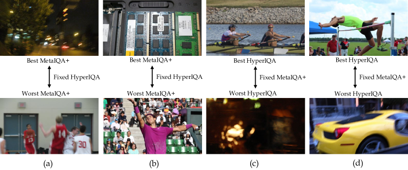
Figure 2: Representative gMAD pairs between HyperIQA and MetaIQA+. (a) Fixing HyperIQA at the low quality level. (b) Fixing HyperIQA at the high quality level. (c) Fixing MetaIQA+ at the low quality level. (d) Fixing MetaIQA+ at the high quality level.

We invite $25$ human subjects ($12$ males and $13$ females) to gather perceived quality judgments of each gMAD pair using the 2AFC method. They are forced to choose the image with higher perceived quality for the $720$ paired comparisons. The $25$ subjects are mostly young researchers (aged between $22$ and $30$) with a computer science background but are unaware of the goal of this work. They are asked to finish the experiments in an office environment with normal lighting conditions and without reflecting ceiling walls and floors.

After subjective testing, we obtain the raw pairwise comparison matrix $A\in\mathbb{R}^{9\times 9}$, where $a_{ij}\in\{0,1\ldots,250\}$ indicates the counts of $x^{\star}$ preferred over $y^{\star}$ by the $25$ subjects on the ten associated image pairs (by solving Problem (4)). We compute, from $A$, a second matrix $B\in\mathbb{R}^{9\times 9}$, where $b_{ij}=a_{ij}/a_{ji}$ denotes the pairwise dominance of $f_{i}$ over $f_{j}$. Laplace smoothing [47] is applied when $a_{ji}$ is close to zero. We convert the pairwise comparisons into a global ranking $r\in\mathbb{R}^{9}$ using Perron rank [48]. A larger $r_{i}$ indicates better performance of $f_{i}$ in the gMAD competition.

Table 2: Ranking results of nine BIQA models. A smaller rank indicates better performance. “Distribution” in the third column means that NIMA uses the earth mover’s distance to match the ground truth and predicted 1D quality distributions. “All” in the fourth column indicates that UNIQUE is trained on the combined dataset of LIVE, CSIQ, KADID-10K, BID, CLIVE, and KonIQ-10K.

Name	Backbone	Formulation	Training Set	Time	SRCC Rank	gMAD Rank	$\Delta$ Rank
UNIQUE [8]	ResNet-34	Ranking	All	2021.03	1	5	-4
KonCept512 [10]	InceptionResNetV2	Regression	KonIQ-10k	2020.01	2	1	1
HyperIQA [7]	ResNet-50	Regression	KonIQ-10k	2020.08	3	2	1
LinearityIQA [15]	ResNeXt-101	Regression	KonIQ-10k	2020.10	4	3	1
MetaIQA+ [46]	ResNet-18	Regression	CLIVE	2021.04	5	8	-3
Fang2020 [21]	ResNet-50	Regression	SPAQ	2020.08	6	9	-3
NIMA [6]	VGG-16	Distribution	AVA	2018.04	7	4	3
DeepIQA [36]	VGG-like CNN	Regression	LIVE	2018.01	8	7	1
RankIQA [5]	VGG-16	Ranking	LIVE	2017.12	9	6	3

Results. Table 2 compares the ranking results of the nine BIQA models in the gMAD competition and in terms of the average SRCC on the four full datasets, BID [19], CLIVE [20], KonIQ-10k [10], and SPAQ [21]. The primary observation is that the latest published models, such as UNIQUE [8], MetaIQA+ [46], and Fang2020 [21] tend to overfit the peculiarities of the training sets with advanced optimization techniques. In particular, UNIQUE learns to rank image pairs from all available datasets, MetaIQA+ adopts deep meta-learning for unseen distortion generalization, while Fang2020 enables multitask learning for incorporation of auxiliary quality-relevant information. They rank much higher in terms of average SRCC than in gMAD.

Compared to improving upon optimization techniques, selecting computational structures with more capacity as the backbones seems to be a wiser choice, as evidenced by KonCept512, HyperIQA, and LinearityIQA with high rankings in gMAD. Figure 2 shows a visual comparison of the representative gMAD pairs between MetaIQA+ based on ResNet-18 and HyperIQA based on ResNet-50. Pairs of images in (a) and (b) have similar quality according to human perception, which is consistent with HyperIQA. When the roles of HyperIQA and MetaIQA+ are reversed, it is clear that the pairs of images in (c) and (d) exhibit substantially different quality. HyperIQA correctly predicts top images to have much better quality than bottom images, and meanwhile, the weaknesses of MetaIQA+ in handling dark and blurry scenes have also been exposed.

3.2 Easy Dataset Problem

In order to reveal the easy dataset problem, it suffices to empirically show that the newly created datasets are less effective in falsifying current BIQA models.

Experimental Setup. We work with the same four datasets - BID [19], CLIVE [20], KonIQ-10k [10], and SPAQ [21]. To achieve our goal, we select a state-of-the-art BIQA model - UNIQUE [8] - that permits training on multiple datasets. We train three UNIQUEs (i.e., UNIQUEv1, UNIQUEv2, and UNIQUEv3, respectively) on the combination of available datasets in chronological order. For each training setting, we randomly sample $80\%$ images from each dataset to construct the training set, leaving the remaining $10\%$ for validation and $10\%$ for testing. To reduce the bias caused by the randomness in dataset splitting, we repeat the training procedure ten times, and report the median SRCC results for UNIQUE variants.

Table 3: SRCC between predictions of UNIQUEs and MOSs of different test sets. “—” means that the corresponding dataset is used for joint training.

SRCC	UNIQUEv1	UNIQUEv2	UNIQUEv3
CLIVE [20]	0.6998	—	—
KonIQ-10k [10]	0.6917	0.7251	—
SPAQ [21]	0.7204	0.7932	0.8112

Results. Table 3 lists the SRCC results between predictions of UNIQUEs and MOSs of different IQA datasets as test sets. The primary observation is that as more datasets are available for training, the newly created datasets are more difficult to challenge the most recently trained UNIQUE version. For example, trained on the combination of BID, CLIVE, and KonIQ-10k, UNIQUEv3 achieves a satisfactory SRCC of $0.8112$ on SPAQ, which is higher than $0.7932$ and $0.7204$ for UNIQUEv2 and UNIQUEv1 trained with fewer data. Although SPAQ is the latest dataset, it is easier than CLIVE and KonIQ-10k, which is supported by the highest correlations obtained by UNIQUEv1 and UNIQUEv2 on SPAQ. These results are consistent with the observations in Sec. 3.1, where models trained on KonIQ-10k and CLIVE rank higher than models trained on SPAQ. What is worse, the most difficult examples (as measured by the mean squared error (MSE) between model predictions and MOSs) often share similar visual appearances (see visual examples in Figure 3). This shows that the sample diversity and difficulty of existing datasets may not be well imposed in a principled way.

(a)

(b)

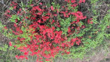
(c)

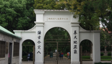
(d)

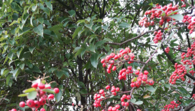
(e)

(f)

(g)

(h)

(i)

(j)

(k)

(l)

(m)

(n)

(o)

Figure 3: The top-5 difficult samples in SPAQ, as measured by the MSE between model predictions and MOSs: (a)-(e) for UNIQUEv1. (f)-(j) for UNIQUEv2. (k)-(o) for UNIQUEv3.

4 Integrating Model-Centric and Data-Centric IQA

In this section, we describe a computational framework for integrating model-centric and data-centric IQA approaches and provide a specific instance within the framework to alleviate the overfitting and easy dataset problems.

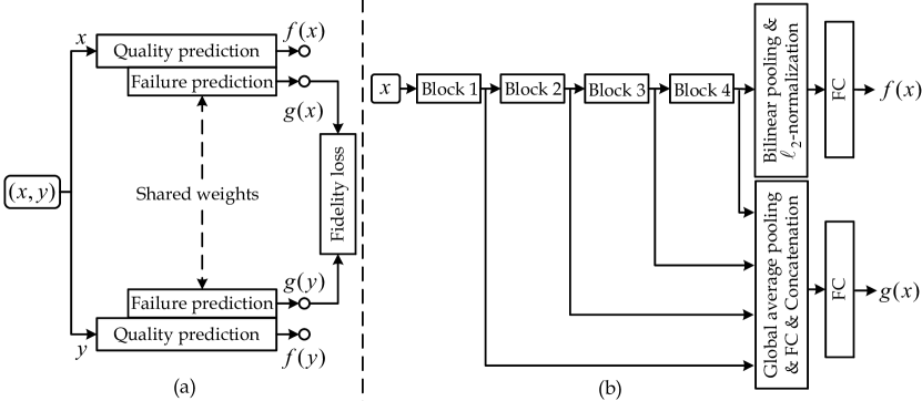
Figure 4: (a) The main quality predictor, $f(\cdot)$, is fixed and the auxiliary failure predictor, $g(\cdot)$, is optimized by minimizing the fidelity loss. (b) The backbone of $f(\cdot)$ is ResNet-34, composed of four residual blocks.

4.1 Proposed Framework

As shown in Figure 1, there is a rich body of work on how to train IQA models on available human-rated datasets, i.e., the connection from data-centric IQA to model-centric IQA. The missing part for closing the loop is to leverage existing IQA models to guide the creation of new IQA datasets. Assuming that a subjective testing environment exists, in which reliable MOSs can be collected, the problem reduces to how to sample, from a large-scale unlabeled dataset $\mathcal{U}$ with great scene complexities and visual distortions, a subset $\mathcal{D}$, whose size is constrained by the human labeling budget. Motivated by the experimental results in Sec. 3, we argue that the images in $\mathcal{D}$ are sampling-worthy if they are difficult and diverse. Mathematically, sample selection corresponds to the following optimization problem:

$$\mathcal{D}=\operatorname*{arg\,max}_{\mathcal{S}\subset{\mathcal{U}}}\mathrm{Diff}(\mathcal{S};f)+\lambda\mathrm{Div}(\mathcal{S}),$$ (5)

where $\mathrm{Diff}(\cdot)$ is a difficulty measure of $\mathcal{S}$ w.r.t. the IQA model, $f(\cdot)$. It is straightforward to define $\mathrm{Diff}(\cdot)$ on a set of IQA algorithms as well. $\mathrm{Div}(\cdot)$ quantifies the diversity of $\mathcal{S}$. $\lambda$ is a trade-off parameter for the two terms. As a specific case of subset selection [49, 50], Problem (5) is generally NP-hard unless special properties of $\mathrm{Diff}(\cdot)$ and $\mathrm{Div}(\cdot)$ can be exploited. Popular approximate solutions to subset selection include greedy algorithms and convex relaxation methods.

Once $\mathcal{D}$ is identified, we collect the MOS for each $x\in\mathcal{D}$ in the assumed subjective testing environment, which makes the connection from model-centric IQA to data-centric IQA. The newly labeled $\mathcal{D}$, by construction, exposes different failures of the IQA model $f(\cdot)$, which is useful for improving its generalization. We then iterate the process of model rectification, sample selection, and subjective testing, with the ultimate goal of improving learning-based IQA from both model and data perspectives.

4.2 A Specific Instance in BIQA

In this subsection, we provide a specific instance of the proposed computational framework, and demonstrate its feasibility in integrating model-centric and data-centric BIQA.

To better contrast with the results in Sec. 3.2 and reduce subjective testing load, we use SPAQ to simulate the large-scale unlabeled dataset $\mathcal{U}$. The off-the-shelf BIQA model for demonstration is again UNIQUE [8], which trains on the combination of the full BID, CLIVE, and KonIQ-10k. The objective function used for optimization is the fidelity loss [42]. The optimization technique is a variant of stochastic gradient descent [51].

The core of our method is the instantiation of the sampling-worthiness module, which consists of two computational submodules to quantify the difficulty of a candidate set $\mathcal{S}$ w.r.t. to $f(\cdot)$ and the diversity of $\mathcal{S}$. Inspired by previous seminal work [52, 53, 54, 55], we measure the difficulty through failure prediction. As shown in Figure 4, our failure predictor, $g(\cdot)$, has two characteristics: 1) it is an auxiliary module that incurs a small number of parameters; 2) it can either be solely trained while holding the quality predictor $f(\cdot)$ fixed or jointly trained along with $f(\cdot)$. Recall that our goal is to expose diverse failures of existing BIQA models, and thus it is preferred not to re-train or fine-tune $f(\cdot)$. For the subsequent experiments, we choose to fix the quality predictor.

Table 4: SRCC results of the proposed sampling-worthiness module against six competing methods with and without the diversity measure. The large-scale unlabeled set $\mathcal{U}$ is simulated with SPAQ [21]. A lower SRCC in $\mathcal{D}$ indicates a stronger capability of failure identification. RD: Representativeness-diversity.

Method	Without diversity		With diversity
	$\mathcal{D}$	$\mathcal{U}\setminus\mathcal{D}$	$\mathcal{D}$	$\mathcal{U}\setminus\mathcal{D}$
Random sampling	0.8452	0.8382	0.8373	0.8383
Sampling by RD [33]	0.5932	0.8383	0.5575	0.8381
UNIQUE uncertainty [8]	0.5633	0.8397	0.5477	0.8400
Query by committee [56]	0.5487	0.8395	0.5352	0.8395
Core-set selection [31]	0.4968	0.8396	0.3796	0.8398
MC dropout [30]	0.4902	0.8376	0.3841	0.8379
Proposed	0.1894	0.8362	0.1413	0.8364

The failure predictor $g(\cdot)$ accepts the feature maps of the input image $x$ from each fixed residual block as inputs, and summarizes spatial information via global average pooling. Each stage of pooled features then undergoes an FC layer with the same number of output channels, $C$, followed by ReLU nonlinearity. After that, the four feature vectors of the same length are concatenated to pass through another FC layer to compute a scalar $g(x)$ as the indication of the difficulty of learning $x$. Assuming Gaussianity of $g(x)$ with unit variance, the probability that $x$ is more difficult than $y$ is calculated by

$$\hat{p}_{\mathrm{F}}(x,y)\ =\ \Phi\left(\frac{g(x)-g(y)}{\sqrt{2}}\right).$$ (6)

For the same training pair $(x,y)$, the ground-truth label can be computed by

$$p_{\mathrm{F}}(x,y)=\begin{cases}1\quad\mbox{if}\,\ |f(x)-\mu(x)|\geq|f(y)-\mu(y)|,\\ 0\quad\mbox{otherwise},\end{cases}$$ (7)

where $\mu(\cdot)$ represents the MOS. That is, $p_{\mathrm{F}}(x,y)=1$ indicates that $x$ is more difficult to learn than $y$, as evidenced by a higher absolute error. We learn the parameters of the failure predictor (i.e., five FC layers) by minimizing the fidelity loss between $p_{\mathrm{F}}(x,y)$ and $\hat{p}_{\mathrm{F}}(x,y)$:

$$\ \ell(x,y,p_{\mathrm{F}})=1-\sqrt{p_{\mathrm{F}}(x,y)\hat{p}_{\mathrm{F}}(x,y)}-\sqrt{(1-p_{\mathrm{F}}(x,y))(1-\hat{p}_{\mathrm{F}}(x,y))}.$$ (8)

One significant advantage of the learning-to-rank formulation of failure prediction is that $g(\cdot)$ is independent of the scale of $f(\cdot)$, which may oscillate over iterations [55] if joint training is enabled. After sufficient training, we may adopt $g(\cdot)$ to quantify the difficulty of $\mathcal{S}$:

$$\mathrm{Diff}(\mathcal{S})=\frac{1}{|\mathcal{S}|}\sum_{x\in\mathcal{S}}g(x),$$ (9)

where $|\mathcal{S}|$ denotes the cardinality of the set $\mathcal{S}$. We next define the diversity of $\mathcal{S}$ as the mean pairwise distances computed from the $1,000$-dim logits of the VGGNet [29]:

$$\mathrm{Div}(\mathcal{S})=\frac{1}{|\mathcal{S}|^{2}}\sum_{(x,y)\in\mathcal{S}}\left\|\mathrm{logit}(x)-\mathrm{logit}(y)\right\|_{2}^{2},$$ (10)

which provides a reasonable account for the semantic dissimilarity. While maximizing $\mathrm{Diff}(\mathcal{S})$ in Eq. (9) enjoys a linear complexity in the problem size, it is not the case when maximizing $\mathrm{Div}(\mathcal{S})$ [57]. To facilitate subset selection, we use a similar greedy method (in Eq. (4)) to solve Problem (5). Assuming $\mathcal{D}=\{x_{k^{\prime}}^{\star}\}_{k^{\prime}=1}^{k-1}$ is the (sub)-optimal subset that contains $k-1$ images, the $k$-th optimal image can be chosen by

$$x_{k}^{\star}=\operatorname*{arg\,max}_{x\in\mathcal{U}\setminus\mathcal{D}}g(x)+\frac{\lambda}{k-1}\sum_{k^{\prime}=1}^{k-1}\left\|\mathrm{logit}(x)-\mathrm{logit}(x_{k^{\prime}}^{\star})\right\|_{2}^{2}.$$ (11)

4.3 Experiments

Experimental Setup. Training is carried out by minimizing the fidelity loss in Eq. (8) for failure prediction while fixing the quality predictor. The output channel of the four FC layers for feature projection is set to $C=128$. All five FC layers in $g(\cdot)$ are initialized by He’s method [58]. We adopt Adam [51] with a mini-batch size of $32$, an initial learning rate of $10^{-4}$ and a decay factor of $10$ for every five epochs, and we train the failure predictor for fifteen epochs. During sample selection, we set the $\lambda$ in Eq. (5) to $10^{-6}$ in order to balance the scale difference between $\mathrm{Diff}(\cdot)$ and $\mathrm{Div}(\cdot)$. We use SPAQ to simulate $\mathcal{U}$ and select a subset $\mathcal{D}$ of size $100$. Similarly, we repeat the training procedure five times and report the median results. We compare the failure identification capability of the proposed sampling-worthiness module against several deep active learning methods, including random sampling, sampling by representativeness-diversity [33], UNIQUE uncertainty [8], query by committee [56], core-set selection [31], and MC dropout [30].

Failure Identification Results. Table 4 shows the SRCC results between UNIQUE predictions and MOSs on the selected $\mathcal{D}$ and the remaining $\mathcal{U}\setminus\mathcal{D}$. A lower SRCC in $\mathcal{D}$ indicates better failure identification performance. We find that, for all methods except random sampling, the selected images in $\mathcal{D}$ are more difficult than the remaining ones. The proposed sampling-worthiness module delivers the best performance, identifying significantly more difficult samples. It is interesting to note that the failure identification performance of all methods, including the proposed failure predictor, can be enhanced by the incorporation of the diversity measure.

(a)

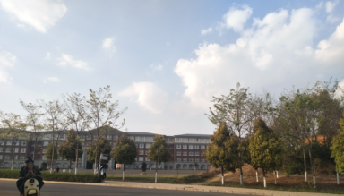
(b)

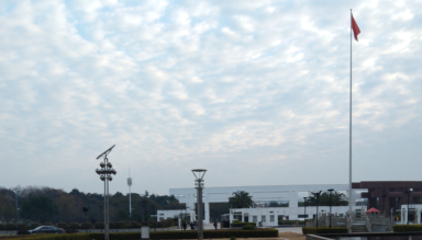
(c)

(d)

(e)

(f)

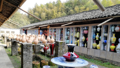
(g)

(h)

Figure 5: Representative images selected from SPAQ by the proposed sampling-worthiness module. (a)-(d)/(e)-(h) are selected images without/with the diversity measure.

Visual Results. Figure 5 shows representative top-$K$ images selected from SPAQ by the proposed sampling-worthiness module. Without the diversity constraint, the failure predictor is inclined to select difficult images of similar visual appearances, corresponding to the same underlying failure cause. When the diverse constraint is imposed, the selected images are more diverse in content and distortion.

5 Conclusion and Future Work

In this paper, we first conducted computational studies to reveal the overfitting problem and the easy dataset problem rooted in the current development of BIQA. We believe these arise because of the weak connections from the model to the data. We then proposed a computational framework to integrate model-centric and data-centric IQA. We also provided a specific instance by developing a sampling-worthiness module for difficulty and diversity quantification. Our module has been proven flexible and effective in spotting diverse failures of BIQA models.

In the future, we will improve the current sampling-worthiness module by developing better difficulty and diversity measures. We may also search for more efficient discrete optimization techniques to solve the subset selection problem in the context of IQA. Moreover, we will certainly leverage the sampling-worthiness module to construct a large-scale challenging IQA dataset, with the goal of facilitating the development of more generalizable IQA models. Last, we hope the proposed computational framework will inspire researchers in related fields to rethink the exciting future directions of IQA.

References

- Ye et al. [2012] Peng Ye, Jayant Kumar, Le Kang, and David Doermann. Unsupervised feature learning framework for no-reference image quality assessment. In IEEE Conference on Computer Vision and Pattern Recognition, pages 1098–1105, 2012.
- Xu et al. [2016] Jingtao Xu, Peng Ye, Qiaohong Li, Haiqing Du, Yong Liu, and David Doermann. Blind image quality assessment based on high order statistics aggregation. IEEE Transactions on Image Processing, 25(9):4444–4457, 2016.
- Ma et al. [2017a] Kede Ma, Wentao Liu, Tongliang Liu, Zhou Wang, and Dacheng Tao. dipIQ: Blind image quality assessment by learning-to-rank discriminable image pairs. IEEE Transactions on Image Processing, 26(8):3951–3964, 2017a.
- Mittal et al. [2012] Anish Mittal, Anush K Moorthy, and Alan C Bovik. No-reference image quality assessment in the spatial domain. IEEE Transactions on Image Processing, 21(12):4695–4708, 2012.
- Liu et al. [2017] Xialei Liu, Joost van de Weijer, and Andrew D Bagdanov. RankIQA: Learning from rankings for no-reference image quality assessment. In IEEE International Conference on Computer Vision, pages 1040–1049, 2017.
- Talebi and Milanfar [2018] Hossein Talebi and Peyman Milanfar. NIMA: Neural image assessment. IEEE Transactions on Image Processing, 27(8):3998–4011, 2018.
- Su et al. [2020] Shaolin Su, Qingsen Yan, Yu Zhu, Cheng Zhang, Xin Ge, Jinqiu Sun, and Yanning Zhang. Blindly assess image quality in the wild guided by a self-adaptive hyper network. In IEEE Conference on Computer Vision and Pattern Recognition, pages 3667–3676, 2020.
- Zhang et al. [2021] Weixia Zhang, Kede Ma, Guangtao Zhai, and Xiaokang Yang. Uncertainty-aware blind image quality assessment in the laboratory and wild. IEEE Transactions on Image Processing, 30(258):3474–3486, 2021.
- Kang et al. [2014] Le Kang, Peng Ye, Yi Li, and David Doermann. Convolutional neural networks for no-reference image quality assessment. In IEEE Conference on Computer Vision and Pattern Recognition, pages 1733–1740, 2014.
- Hosu et al. [2020] Vlad Hosu, Hanhe Lin, Tamas Sziranyi, and Dietmar Saupe. KonIQ-10k: An ecologically valid database for deep learning of blind image quality assessment. IEEE Transactions on Image Processing, 29(305):4041–4056, 2020.
- Ma et al. [2017b] Kede Ma, Wentao Liu, Kai Zhang, Zhengfang Duanmu, Zhou Wang, and Wangmeng Zuo. End-to-end blind image quality assessment using deep neural networks. IEEE Transactions on Image Processing, 27(3):1202–1213, 2017b.
- Zhang et al. [2020] Weixia Zhang, Kede Ma, Jia Yan, Dexiang Deng, and Zhou Wang. Blind image quality assessment using a deep bilinear convolutional neural network. IEEE Transactions on Circuits and Systems for Video Technology, 30(1):36–47, 2020.
- Gao et al. [2015] Fei Gao, Dacheng Tao, Xinbo Gao, and Xuelong Li. Learning to rank for blind image quality assessment. IEEE Transactions on Neural Networks and Learning Systems, 26(10):2275–2290, 2015.
- Liu [2011] Tie-Yan Liu. Learning to Rank for Information Retrieval. Springer Science & Business Media, 2011.
- Li et al. [2020] Dingquan Li, Tingting Jiang, and Ming Jiang. Norm-in-norm loss with faster convergence and better performance for image quality assessment. In ACM International Conference on Multimedia, pages 789–797, 2020.
- Wang et al. [2021] Zhihua Wang, Dingquan Li, and Kede Ma. Semi-supervised deep ensembles for blind image quality assessment. In International Joint Conference on Artificial Intelligence Workshop on Weakly Supervised Representation Learning, pages 1–6, 2021.
- Li [2017] Mu Li. Scaling Distributed Machine Learning with System and Algorithm Co-design. PhD thesis, Carnegie Mellon University, 2017.
- Sheikh et al. [2006] Hamid R Sheikh, Muhammad F Sabir, and Alan C Bovik. A statistical evaluation of recent full reference image quality assessment algorithms. IEEE Transactions on Image Processing, 15(11):3440–3451, 2006.
- Ciancio et al. [2011] Alexandre Ciancio, André Luiz N Targino da Costa, Eduardo A B da Silva, Amir Said, Ramin Samadani, and Pere Obrador. No-reference blur assessment of digital pictures based on multifeature classifiers. IEEE Transactions on Image Processing, 20(1):64–75, 2011.
- Ghadiyaram and Bovik [2016] Deepti Ghadiyaram and Alan C Bovik. Massive online crowdsourced study of subjective and objective picture quality. IEEE Transactions on Image Processing, 25(1):372–387, 2016.
- Fang et al. [2020] Yuming Fang, Hanwei Zhu, Yan Zeng, Kede Ma, and Zhou Wang. Perceptual quality assessment of smartphone photography. In IEEE Conference on Computer Vision and Pattern Recognition, pages 3677–3686, 2020.
- Mantiuk et al. [2012] Rafał K Mantiuk, Anna Tomaszewska, and Radosław Mantiuk. Comparison of four subjective methods for image quality assessment. Computer Graphics Forum, 31(8):2478–2491, 2012.
- Xu et al. [2012] Qianqian Xu, Qingming Huang, Tingting Jiang, Bowei Yan, Weisi Lin, and Yuan Yao. HodgeRank on random graphs for subjective video quality assessment. IEEE Transactions on Multimedia, 14(3):844–857, 2012.
- Ye and Doermann [2014] Peng Ye and David Doermann. Active sampling for subjective image quality assessment. In IEEE Conference on Computer Vision and Pattern Recognition, pages 4249–4256, 2014.
- Vonikakis et al. [2017] Vassilios Vonikakis, Ramanathan Subramanian, Jonas Arnfred, and Stefan Winkler. A probabilistic approach to people-centric photo selection and sequencing. IEEE Transactions on Multimedia, 19(11):2609–2624, 2017.
- Cao et al. [2021] Peibei Cao, Zhangyang Wang, and Kede Ma. Debiased subjective assessment of real-world image enhancement. In IEEE Conference on Computer Vision and Pattern Recognition, pages 711–721, 2021.
- Wang and Simoncelli [2008] Zhou Wang and Eero P Simoncelli. Maximum differentiation (MAD) competition: A methodology for comparing computational models of perceptual quantities. Journal of Vision, 8(12):1–13, 2008.
- Wang et al. [2020] Haotao Wang, Tianlong Chen, Zhangyang Wang, and Kede Ma. I am going MAD: Maximum discrepancy competition for comparing classifiers adaptively. In International Conference on Learning Representations, pages 1–13, 2020.
- Simonyan and Zisserman [2015] Karen Simonyan and Andrew Zisserman. Very deep convolutional networks for large-scale image recognition. In International Conference on Learning Representations, pages 1–14, 2015.
- Pop and Fulop [2018] Remus Pop and Patric Fulop. Deep ensemble Bayesian active learning: Addressing the mode collapse issue in Monte Carlo dropout via ensembles. arXiv preprint arXiv:1811.03897, 2018.
- Sener and Savarese [2018] Ozan Sener and Silvio Savarese. Active learning for convolutional neural networks: A core-set approach. In International Conference on Learning Representations, pages 1–13, 2018.
- Burbidge et al. [2007] Robert Burbidge, Jem J Rowland, and Ross D King. Active learning for regression based on query by committee. In International Conference on Intelligent Data Engineering and Automated Learning, pages 209–218, 2007.
- Wu [2019] Dongrui Wu. Pool-based sequential active learning for regression. IEEE Transactions on Neural Networks and Learning Systems, 30(5):1348–1359, 2019.
- Moorthy and Bovik [2011] Anush K Moorthy and Alan C Bovik. Blind image quality assessment: From natural scene statistics to perceptual quality. IEEE Transactions on Image Processing, 20(12):3350–3364, 2011.
- Saad et al. [2012] Michele A Saad, Alan C Bovik, and Christophe Charrier. Blind image quality assessment: A natural scene statistics approach in the DCT domain. IEEE Transactions on Image Processing, 21(8):3339–3352, 2012.
- Bosse et al. [2018] Sebastian Bosse, Dominique Maniry, Klaus-Robert Müller, Thomas Wiegand, and Wojciech Samek. Deep neural networks for no-reference and full-reference image quality assessment. IEEE Transactions on Image Processing, 27(1):206–219, 2018.
- ITU-R Recommendation [2019] ITU-R Recommendation. BT.500-14: Methodologies for the subjective assessment of the quality of television images, 2019. URL https://www.itu.int/dms_pubrec/itu-r/rec/bt/R-REC-BT.500-14-201910-S!!PDF-E.pdf.
- Men et al. [2021] Hui Men, Hanhe Lin, Mohsen Jenadeleh, and Dietmar Saupe. Subjective image quality assessment with boosted triplet comparisons. IEEE Access, 9:138939–138975, 2021.
- Ponomarenko et al. [2009] Nikolay Ponomarenko, Vladimir Lukin, Alexander Zelensky, Karen Egiazarian, Marco Carli, and Federica Battisti. TID2008 - A database for evaluation of full-reference visual quality assessment metrics. Advances of Modern Radioelectronics, 10(4):30–45, 2009.
- Larson and Chandler [2010] Eric C Larson and Damon M Chandler. Most apparent distortion: Full-reference image quality assessment and the role of strategy. Journal of Electronic Imaging, 19(1):1–21, 2010.
- Ying et al. [2020] Zhenqiang Ying, Haoran Niu, Praful Gupta, Dhruv Mahajan, Deepti Ghadiyaram, and Alan C Bovik. From patches to pictures (PaQ-2-PiQ): Mapping the perceptual space of picture quality. In IEEE Conference on Computer Vision and Pattern Recognition, pages 3575–3585, 2020.
- Tsai et al. [2007] Ming-Feng Tsai, Tie-Yan Liu, Tao Qin, Hsin-Hsi Chen, and Wei-Ying Ma. FRank: A ranking method with fidelity loss. In International ACM SIGIR Conference on Research and Development in Information Retrieva, pages 383–390, 2007.
- He et al. [2016] Kaiming He, Xiangyu Zhang, Shaoqing Ren, and Jian Sun. Deep residual learning for image recognition. In IEEE Conference on Computer Vision and Pattern Recognition, pages 770–778, 2016.
- Goodfellow et al. [2016] Ian Goodfellow, Yoshua Bengio, and Aaron Courville. Deep Learning. MIT Press, 2016.
- Ma et al. [2020] Kede Ma, Zhengfang Duanmu, Zhou Wang, Qingbo Wu, Wentao Liu, Hongwei Yong, Hongliang Li, and Lei Zhang. Group maximum differentiation competition: Model comparison with few samples. IEEE Transactions on Pattern Analysis and Machine Intelligence, 42(4):851–864, 2020.
- Zhu et al. [2022] Hancheng Zhu, Leida Li, Jinjian Wu, Weisheng Dong, and Guangming Shi. Generalizable no-reference image quality assessment via deep meta-learning. IEEE Transactions on Circuits and Systems for Video Technology, 32(3):1048–1060, 2022.
- Manning et al. [2008] Christopher D Manning, Prabhakar Raghavan, and Hinrich Schütze. Introduction to Information Retrieval. Cambridge University Press, 2008.
- Saaty and Vargas [1984] Thomas L Saaty and Luis G Vargas. Inconsistency and rank preservation. Journal of Mathematical Psychology, 28(2):205–214, 1984.
- Davis et al. [1997] Geoff Davis, Stephane Mallat, and Marco Avellaneda. Adaptive greedy approximations. Constructive Approximation, 13(1):57–98, 1997.
- Natarajan [1995] Balas Kausik Natarajan. Sparse approximate solutions to linear systems. SIAM Journal on Computing, 24(2):227–234, 1995.
- Kingma and Ba [2015] Diederik P Kingma and Jimmy Ba. Adam: A method for stochastic optimization. In International Conference on Learning Representations, pages 1–15, 2015.
- Welling [2009] Max Welling. Herding dynamical weights to learn. In International Conference on Machine Learning, pages 1121–1128, 2009.
- Elhamifar and Vidal [2013] Ehsan Elhamifar and René Vidal. Sparse subspace clustering: Algorithm, theory, and applications. IEEE Transactions on Pattern Analysis and Machine Intelligence, 35(11):2765–2781, 2013.
- Misra et al. [2014] Ishan Misra, Abhinav Shrivastava, and Martial Hebert. Data-driven exemplar model selection. In IEEE Winter Conference on Applications of Computer Vision, pages 339–346, 2014.
- Yoo and Kweon [2019] Donggeun Yoo and In So Kweon. Learning loss for active learning. In IEEE Conference on Computer Vision and Pattern Recognition, pages 93–102, 2019.
- Seung et al. [1992] H Sebastian Seung, Manfred Opper, and Haim Sompolinsky. Query by committee. In Annual Workshop on Computational Learning Theory, pages 287–297, 1992.
- Kuo et al. [1993] Ching-Chung Kuo, Fred Glover, and Krishna S Dhir. Analyzing and modeling the maximum diversity problem by zero-one programming. Decision Sciences, 24(6):1171–1185, 1993.
- He et al. [2015] Kaiming He, Xiangyu Zhang, Shaoqing Ren, and Jian Sun. Delving deep into rectifiers: Surpassing human-level performance on ImageNet classification. In IEEE International Conference on Computer Vision, pages 1026–1034, 2015.