A multiwavelength study of the flat spectrum radio-quasar NVSS J141922-083830 covering four flaring episodes

Abstract

We present multiwavelength observations and a model for flat spectrum radio quasar NVSS J141922-083830, originally classified as a blazar candidate of unknown type (BCU II object) in the Third Fermi-LAT AGN Catalog (3LAC). Relatively bright flares (>3 magnitudes) were observed on 21 February 2015 (MJD 57074) and 8 September 2018 (MJD 58369) in the optical band with the MASTER Global Robotic Net (MASTER-Net) telescopes. Optical spectra obtained with the Southern African Large Telescope (SALT) on 1 March 2015 (MJD 57082), during outburst, and on 30 May 2017 (MJD 57903), during quiescence, showed emission lines at 5325Å and at $\approx$3630Å that we identified as the Mg ii 2798Å and C iii] 1909Å lines, respectively, and hence derived a redshift $z$ = 0.903. Analysis of Fermi-LAT data was performed in the quiescent regime (5 years of data) and during four prominent flaring states in February–April 2014, October–November 2014, February–March 2015 and September 2018. We present spectral and timing analysis with Fermi-LAT. We report a hardening of the gamma-ray spectrum during the last three flaring periods, with a power-law spectral index $\Gamma=2.0$–$2.1$. The maximum gamma-ray flux level was observed on 24 October 2014 (MJD 56954) at $(7.57\pm 1.83)\times 10^{-7}$ ph cm^-2s^-1. The multi-wavelength spectral energy distribution during the February–March 2015 flare supports the earlier evidence of this blazar to belong to the FSRQ class. The SED can be well represented with a single-zone leptonic model with parameters typical of FSRQs, but also a hadronic origin of the high-energy emission can not be ruled out.

1 Introduction

An active galactic nucleus (AGN) is a compact structure at the centre of a massive galaxy (usually elliptical). It consists of a super-massive black hole (SMBH, M $\sim$ $10^{6}-10^{10}$ solar masses) surrounded by an accretion disk of plasma that emits thermal radiation $-$ mainly in the UV $-$ produced by the strong gravitational potential of the central SMBH on the plasma particles. Several classes of objects that were discovered or classified throughout the past decades $-$ radio-galaxies, Seyfert galaxies, then quasars and blazars $-$ are today discussed within the framework of the unified model of AGNs (Urry & Padovani, 1995). AGNs are classified into many classes and subclasses, and they may appear to the observers as objects with different properties, due to their distance, their position with respect to their observation direction, or their physical properties. However, it is most likely that they are all the same type of objects, but viewed through different angles and/or at different stages of their evolution. Quasi stellar radio sources (quasars) and quasi stellar objects (QSOs) are the most distant AGNs, since they are often seen as point-like objects, outshining their host galaxy which is often too faint to be detected. Radio emission from AGNs comes from a pair of Doppler-boosted jets of relativistic plasma, understood to be initiated by a spinning SMBH in a strong magnetic field ($\geq 1$ G). These jets are typically perpendicular to the accretion disk and are pointing in opposite directions. We focus in this paper on the blazar class, radio-loud AGNs that are seen close to the direction of one of their jets.

Blazars are classified into two subclasses: flat spectrum radio quasars (FSRQs) and BL Lac objects. Most of the radiation detected from blazars is non-thermal emission produced within the jets, and spreads over the whole electromagnetic spectrum, from radio waves to gamma rays. The spectral energy distributions (SEDs) of blazars exhibit a characteristic double bump structure. The low-energy bump peaks in the optical–IR, and is understood to be due to synchrotron emission from relativistic electrons of the jets. The high-energy bump typically peaks in the X-ray or gamma-ray domain. The radiation production mechanisms that causes the high-energy bump are still debated. It could be due to inverse Compton scattering of photon fields by some population of electrons which are producing the synchrotron radiation (leptonic models). However, in several instances the data may be better reproduced by hadronic models (proton synchrotron, cascades, etc) — see for example Böttcher et al. (2013). Depending on the frequency of the first peak (also called synchrotron peak $\nu_{pk}^{syn}$), we refer to low, intermediate and high synchrotron peaked objects respectively: LSP ($\nu_{pk}^{syn}<10^{14}Hz$), ISP ($10^{14}<\nu_{pk}^{syn}<10^{15}Hz$) or HSP ($\nu_{pk}^{syn}<10^{15}Hz$) blazars. On average, FSRQs are more energetic than BL Lacs. They are seen at higher redshifts, and present a more dramatic variability pattern (Chiaro et al., 2016), though some observational bias may be responsible for this trend. More specifically, FSRQs are surrounded by a relatively dense shell of gas and radiation (typically $\sim$ 0.2 pc from the SMBH), which is called the broad-line region (BLR), due to the high velocity of these “clouds” that cause a Doppler broadening of the emission lines in the optical spectrum of the blazar. Consequently, it is easier to determine the redshifts of FSRQs, than those of BL Lacs whose spectra are often quasi featureless (their optical lines having an equivalent width $<$ 5 Å in their rest frame). Most of the FSRQs belong to the LSP category, and rarely to the ISP category, though BL Lacs are fairly uniformly distributed within the three LSP, ISP and HSP categories (Abdo et al., 2010b).

The study of blazars is of particular importance for astrophysics and cosmology, as well as for particle and plasma physics. Physical processes involved in blazars under extreme conditions of acceleration, density, magnetic and gravitational fields can be probed only in such objects. Also, since the redshifts of gamma-ray blazars spread from $\sim$0.1 to $>$5, blazar populations constitute probes to study the evolution of galaxies throughout the history of the Universe. Improvement in the blazar classification is then of significant importance for addressing the physical, astrophysical and cosmological challenges mentioned above.

The Fermi Gamma-Ray Space Telescope has orbited the Earth since June 2008. It operates in survey mode for most of the time, covering the whole sky every 3 h (corresponding to two orbits), thanks to its 2.4-sr field of view. This allows a regular monitoring of sources on the whole sky. However, due to a technical problem with the spacecraft, scientific operations were interrupted from 16 March till 8 April 2018. Fermi resumed its mission from this date in partial sky-scanning mode. Its main instrument, the Large Area Telescope (LAT), is sensitive to photons from $\sim$20 MeV to $>300$ GeV (Atwood et al., 2009).

During the first ten years of observation (2008–2018), 5788 sources above 4 $\sigma$ significance were detected above 50 MeV and were reported in the Fourth Fermi-LAT point source catalogue – Data Release 2 (Abdollahi et al., 2020; Ballet et al., 2020, 4FGL–DR2). Among these sources, 3492 were identified as AGNs and are recorded in the Fourth Fermi-LAT AGN Catalog – Data Release 2 (Ajello et al., 2020; Lott et al., 2020, 4LAC–DR2). Most of the 4LAC–DR2 objects are blazars (3420 sources–including both the high and low Galactic latitude samples): 1190 BL Lacs, 733 FSRQs and 1497 blazar candidates of uncertain type (BCUs). In the Fermi-LAT Third AGN Catalog (3LAC), BCUs are defined as objects that were categorised as blazars by other means than a detailed optical spectrum, and so are not yet classified as a BL Lac or FSRQ (Ackermann et al., 2015). BCUs are subdivided into three subclasses — from I to III, “BCU I” being the class with more information on the source, “BCU III” the class with the least information:

1. BCUs I: A published optical spectrum of the object is available, but not sensitive enough for a classification as an FSRQ or a BL Lac. Redshifts are often known.

2. BCUs II: the object lacks an optical spectrum, but a reliable position of the SED synchrotron peak can be determined. Redshifts are not known.

3. BCUs III: the object is lacking both an optical spectrum and an estimated synchrotron-peak position, but it shows blazar-like broadband emission and a flat radio spectrum. Redshift are not known.

NVSS J141922–083830 is a radio source from the NRAO VLA Sky Survey (NVSS) catalogue (Condon et al., 1998), and is also recorded as WISE J141922.55-083832.0 in the catalogue of the Wide-field Infrared Survey Explorer in mid-infrared bands (Cutri & et al., 2012). It was classified as a BCU II in the 3LAC and although not a bright Fermi source, it was reported in the Second Fermi-LAT point source catalogue (Nolan et al., 2012, 2FGL), from 2 years of observations, at a significance level of $\sim 7\sigma$ (2FGL J1419.4-0835). In the Third Fermi-LAT point source catalogue (Acero et al., 2015, 3FGL), from 4 years of observations, it has a significance level of $\sim 15\sigma$ (3FGL J1419.5-0836). Finally in the 4FGL and 4FGL–DR2 catalogues, from 8 and 10 years of observation, respectively, NVSS J141922–083830 is labeled as 4FGL J1419.4-0838 and has a significance of $\sim 47$ and $\sim 54\sigma$, respectively (Abdollahi et al., 2020; Ballet et al., 2020).

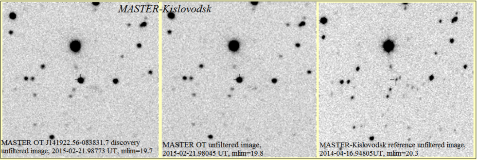
Figure 1: Images taken by MASTER-SAAO network. The first and second panels shows the unfiltered images observed on 21 February 2015 (MJD 57074) at different times, while the third is the reference image taken on 6 February 2014 (MJD 56694). The white-light (filtered) magnitude of NVSS J141922-083830 was measured at 14.6 on 21 February 2015 (MJD 57074.98773, first panel)

.

NVSS J141922–083830 was identified as an LSP source in the Fermi-LAT Second AGN Catalog (Ackermann et al., 2011, 2LAC). In preparation for the 8-year 4LAC, the Fermi-LAT Collaboration performed new broad-band SED fits of many sources, which yielded for this source a synchrotron peak frequency $\nu_{syn}=1.20\times 10^{13}$ Hz at ($\nu F_{\nu})_{syn}=1.33\times 10^{-12}$ erg cm^-2 s^-1 (Ajello et al., 2020). Several interesting studies were undertaken within the previous decade to identify blazar candidates as either BL Lacs or FSRQs from statistical tools using multiwavelength photometry (e.g. D’Abrusco et al., 2014; Chiaro et al., 2016; Chiaro et al., 2018). Though some results were achieved through these methods in identifying NVSS J141922–083830 as an FSRQ at some level of probablity, confirmation was still needed though a more complete study, including optical spectroscopy. We consider that this was achieved through our initial discovery alert (Buckley et al., 2015) with our first optical spectrum, plus the work presented in the current paper. Based on this initial work, the source type is referenced as a FSRQ in the 4FGL and subsequent catalogues.

In February–March 2015, a major flare of this source was discovered in the optical with the MASTER Global Robotic Net (Lipunov et al., 2015), in the near infrared with the Guillermo Haro Observatory (Carrasco et al., 2015) and in X rays with the Niel Gehrels Swift Observatory (Carpenter et al., 2015). Following the MASTER alert, we triggered a spectroscopic observation with the Southern African Large Telescope (SALT). Our analysis of the Fermi-LAT data during this epoch allowed us to observe contemporaneous gamma-ray activity, along with the Swift observations. The broadband emission during this major flare is studied within the framework of theoretical emission models.

The outline of the paper is as follows: in section 2 we present all of the optical observations which includes photometry, polarimetry and spectroscopy; in Section 3 we discuss the Swift XRT and UVOT observations; in Section 4 we present the Fermi-LAT observations and analysis; in Section 5 the SED and spectral modelling results are presented, while finally the summary and conclusions are given in Section 6.

2 Optical Observations and Data Analysis

Here we report on the optical observations of NVSS J141922–083830. These extend over a period of 7.7 years and cover three periods when NVSS J141922–083830 underwent flaring episodes. The optical observations include photometry and polarimetry from three MASTER observatories, in South Africa (MASTER-SAAO), Russia (MASTER-Kislovodsk) and the Canary Islands (MASTER-IAC), plus spectroscopy from SALT.

2.1 MASTER optical observations

The MASTER network (Lipunov et al., 2010) consists of 9 identical fully robotic telescope systems situated at different nodes, five in Russia (MASTER-Amur, -Tunka, -Ural, -Kislovodsk, -Tavrida), MASTER-SAAO at the SAAO, MASTER-IAC in Spain at Instituto de Astrofísica de Canarias (IAC, Tenerife), MASTER-OAFA at the Observatorio Astronomico Felix Aguilar of San Juan National University in Argentina and MASTER-OAGH in Mexico. Each node consists of identical dual 0.4-m diameter wide field telescopes (Hamilton design) on a common mount, with Apogee CCD cameras (4k $\times$ 4k $\times$ 9$\mu$m pixels) with BVRI and clear filters and 2 broad-band polarizers (Kornilov et al., 2012). The telescope tubes can either be co-aligned, each surveying an identical $2^{\circ}\times 2^{\circ}$ field, with two different filters or polarizers, or they can be misaligned to allow twice the sky coverage using identical filters. The latter is the default for the transient survey mode, which is usually done without using a filter to maximize sensitivity (Lipunov et al., 2010, 2019a, 2022; Kornilov et al., 2012).

Each MASTER observatory is controlled by identical automated software (the main MASTER key feature) allowing them to operate as both autonomous fast alert follow-up systems and as survey telescopes for the discovery of astrophysical transients of all classes. Data reduction tasks, which include standard dark, flat field and astrometry calibrations, are performed using the MASTER pipeline software, where dark frames and twilight flats are obtained in automatic mode. Aperture photometry of the object and comparison stars was performed using Photutils (Bradley et al., 2019).

The MASTER software gives information about all optical sources from images 1-2 minutes following CCD readout. This information includes the full classification of all sources from the image, the full dataset from previous MASTER-Net archive images for every sources, the full information from VIZIER database and all open sources (e.g. Minor Planet Center), orbital elements for moving objects, etc. Taking into account the large field of view of the MASTER telescopes 2 x (2^∘ x 2^∘), we have at our disposal a large number ($\approx$ 3000 to 10000) of reference stars to use for photometric reductions. As a result, the photometric errors are minimized. Comparison stars for automatic initial photometry are typically chosen from the USNO-B1 (Monet et al., 2003) catalogue and the USNO magnitudes transform to the MASTER unfiltered system as W=0.2B + 0.8R . Errors are determined from the fitting relations between the standard deviations and magnitudes for the comparison stars(Lipunov et al., 2010; Kornilov et al., 2012; Gorbovskoy et al., 2013).

Each pair of MASTER telescope tubes are equipped with achromatic wire-grid polarizers, mutually perpendicular to one another. In the case of the two MASTER observatories which obtained contemporaneous polarimetry of NVSS J141922–083830 (3$-$5 March 2015), for MASTER-Kislovodsk, the planes are at positional angles 0^∘ and 90^∘ to the celestial equator (this is also the same for MASTER-IAC), while for MASTER-SAAO, the angles are 45^∘ and 135^∘. Using both contemporaneous MASTER observations, with the four different orientations of the polarizers, it is possible to derive the $Q$ and $U$ Stokes parameters and hence the degree of linear polarization and position angle. In spite of the fact that all MASTER telescopes have a similar construction, optical scheme, and polarizers, there are some differences in the CCD responses which limit the precision of the polarization measurements. Also, the calibration using known polarized galactic sources is not possible, since any measurement of polarization involves the subtraction of nearby field stars between at least two images, obtained with tubes with differently oriented polarizers. Thus, the derived polarization of a target object is always relative to the nearby field stars. They are usually chosen from the area around the target source in a radius of 10 arcmin and are bound to have the same polarization due to the similar interstellar matter properties toward them (Kornilov et al., 2012; Gorbovskoy et al., 2016; Lipunov et al., 2019b).

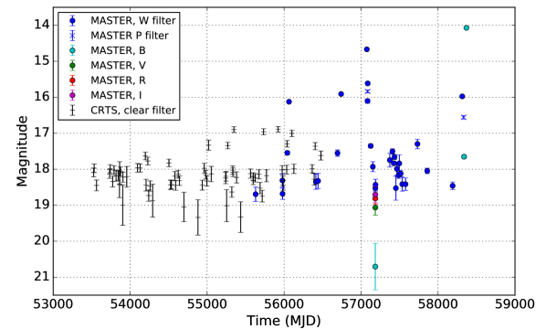
Figure 2: MASTER network light-curves of NVSS J141922-083830, together with measurements from CRTS, all binned in one day intervals.

Lipunov et al. (2015) reported the detection of an optical flare from NVSS J141922–083830 using the MASTER optical transient auto-detection system on 2015-02-21.98773 UTC (MJD 57074.988) as MASTER OT J141922.56-083831.7. The unfiltered flare magnitude was 14.6 and the MASTER-Kislovodsk discovery images plus reference image are shown in Figure 1, The source was seen in 60 previous MASTER images, obtained since 9 March 2011 (MJD 55629). The quiescent brightness values, over 3 years (2011-2014), range from 17$-$19. A total of three additional flares have been detected in MASTER archive images. The unfiltered magnitudes of these flares were 16.1, 15.9 and 14.5$-$16.5, respectively. Flares from NVSS J141922–083830 were first reported from the Catalina Real Time Survey (CRTS; Drake et al., 2009), where it was observed to reach a maximum brightness of V = 16.85 around MJD 55017 (CSS100601:141922-083830; Djorgovski et al., 2010), which are shown in Figure 2.

2.1.1 Followup optical photometry

Followup photometric observations of NVSS J141922–083830 were obtained on MASTER-SAAO and MASTER-Kislovodsk, starting $\approx$9 d after the flare detection (from 2 March 2015/MJD 57083.964, when it appears the Fermi-LAT flux had dropped by a factor of $\approx$2). Simultaneous observations on two optical tubes in the clear $W$ filters were processed as independent observations, while fluxes u sing the two orthogonal polarizers of one MASTER telescope pair were summed as one observation. After this, photometric data processing was performed with Astrokit (Burdanov et al., 2014) to minimize the standard deviation of an ensemble of comparison stars chosen from the Pan-STARRS1 (PS1) catalogue Chambers et al. (2016); Kostov & Bonev (2018).

The day-binned light curve of NVSS J141922–083830 is presented in Figure 2. Errors were determined as the standard deviation of magnitudes in each bin. The longest continuous sets of photometric observations were obtained on 3–4 and 5 March 2015 (MJD 57084–57086). The brightness of the source was seen to slowly decrease during the SAAO 3–4 March observation, while observations on 4 & 5 March showed the source to have brightened by $\approx$ 0.5 magnitude. The light curve over this period is shown in Figure 3.

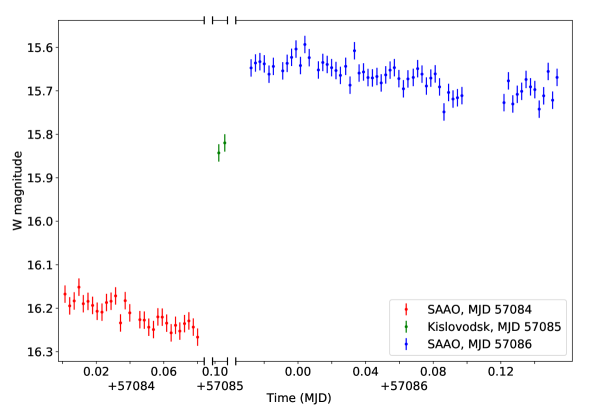
Figure 3: High time resolution light curve based on observations with polarization filters at 3–5 March 2015 (MJD 57084–57086), just past the peak of gamma-ray Flare 3 (see Section 4).

NVSS J141922–083830 was observed briefly on 1 March 2015 (MJD 57082.00) using the SAAO 1.9 m telescope and the SHOC high-speed EM-CCD camera. Measurements confirmed the object was still in a bright flaring state (V $<$ 15), the motivation for a subsequent SALT spectroscopic observation (see Section 2.2).

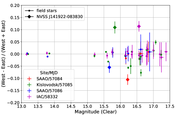
Figure 4: MASTER measurements of normalized Stokes $q$ and $u$ parameters for NVSS J141922-083830 during two flaring episodes, in March 2015 (SAAO (u) and Kislovodsk (q)) and August 2018 (IAC (q)), together with similar measurements for foreground stars in the field. These are determined by taking the ratio of the difference and summed intensities, respectively, observed in each pair of CCD frames corresponding to the orthogonally offset polarizers.

2.1.2 Polarization measurements

Polarimetric observations were carried out in March 2015 and August 2018 with the MASTER-SAAO, MASTER-Kislovodsk and MASTER-IAC observatories. Details are presented in Table 1. We see that NVSS J141922–083830 is consistently polarized, from all four attempted measurements.

The degree of polarization, $P$ was calculated as $(\mathrm{Flux_{West}-Flux_{East})/(Flux_{West}+Flux_{East}})$. The estimated values correspond to normalized Stokes parameters q for Kislovodsk and IAC observations and u for SAAO observations. The results are presented in Figure 4 for both NVSS J141922–083830 and a number of field stars. As can be seen from the plot, only three field stars showed any evidence for being polarized, not surprisingly given the high Galactic latitude ($b$ = 47.83^∘). We also investigated any potential correlations between the measured minimum polarization from the MASTER-SAAO and MASTER-IAC data with Gaia DR2 parallaxes and found none.

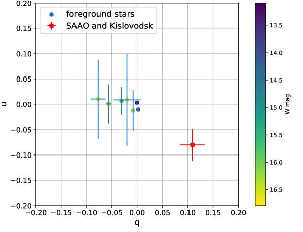
Figure 5: Normalized Stokes $q$ and $u$ parameters determined for NVSS J141922–083830 and nearby field stars during the flare episodes in March 2015 (gamma-ray Flare 3 – see Section 4).

Table 1: Log of polarization observations of NVSS J141922–083830

Observatory	Date Range	MJD range	# of CCD exposure pairs	$|P|$	W magnitude
MASTER-SAAO	2015-03-03.002 to 2015-03-03.080	57084.002–57084.080	29	10.5 $\pm$ 2.2%	16.22 $\pm$ 0.03
MASTER-Kislovodsk	2015-03-04.102 to 2015-03-04.104	57085.102–57085.104	2	10.9 $\pm$ 2.5%	15.83 $\pm$ 0.01
MASTER-SAAO	2015-03-04.972 to 2015-03-05.153	57085.972–57086.153	59	5.5 $\pm$ 2.3%	15.66 $\pm$ 0.03
MASTER-IAC	2018-08-02.880 to 2018-08-02.906	58332.880–58332.906	10	11.4 $\pm$ 2.2%	16.56 $\pm$ 0.04

In the absence of polarimetric observations from two or more MASTER observatories overlapping in time, we can only determine a lower limit for the degree of polarization. Hovever, if we assume a linear change of the degree of polarization, $p$, between the two MASTER-SAAO observations on 3 & 5 March 2015, plus a constant polarization angle, $\theta$, then we derive the mean normalized Stokes parameters for the time of the Kislovodsk polarimetric observation, performed in between the two MASTER-SAAO observations. The combined observations were obtained with 4 angles of the polarizers, namely 0, 45, 90 & 135^∘, which allows us to determine the normalized Stokes $q$ and $u$ parameters for NVSS J141922–083830 and 7 field stars, which are shown in Figure 5. We determined these to be $q=0.109\pm 0.025$ and $u=-0.080\pm 0.031$, implying $p=(13.5\pm 3.9)\%$ and $\theta=(-18.2\pm 12.5)^{\circ}$.

2.2 SALT Optical spectroscopy

An optical spectrum of NVSS J141922–083830 was obtained with SALT (Buckley et al., 2006) on 1 March 2015 (MJD 57082; Buckley et al., 2015), with the Robert Stobie Spectrograph (RSS; Burgh et al., 2003). The PG900 VPH grating was used at a grating angle of 14.0^∘. A 1100 s exposure spectrum, covering 3780–6850Å at a resolution of 4.8Å with a 1.25 arcsec slit, was obtained in clear conditions and seeing of 1.5 arcsec.

The data were reduced using the PySALT package, a PyRAF-based software package for SALT data reductions (Crawford et al., 2010), which includes corrections for both gain and cross-talk, bias subtraction, amplifier mosaicing, and removal of cosmetic defects. The individual spectra were then extracted using standard IRAF procedures, wavelength calibration (with a calibration lamp exposure taken immediately after the science spectra), background subtraction and extraction of 1D spectra. We could only obtain relative flux calibrations, from observing spectrophotometric standards in twilight, due to the SALT design (Buckley et al., 2018).

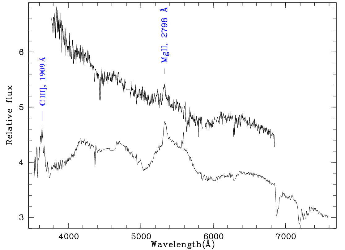
Figure 6: SALT spectra of NVSS J141922-083830 obtained on 1 March 2015 (MJD 57082; upper), 7 days after the flare detection, and 30 May 2017 (MJD 57903; lower), when in quiescence. The emission feature at 5325Å is identified as Mg ii 2798Å, which implies a redshift of z=0.903. The line towards the blue end of the 2017 observation is identified as the C iii] 1909Å line. Note that the flux levels are relative and the 2017 spectrum (lower plot) has been scaled by a factor of 1.5.

The spectrum, included in Figure 6, shows a single emission line at 5325Å with an equivalent width of E.W. = $1.25\pm 0.11$ and line width of FWHM = $28.1\pm 1.8$ Å. The only other spectral features worth commenting on are some very broad ($\sim$500Å) bumps at $\sim$4200, 4600 and 6400Å, superimposed on a continuum which steeply rises to the blue. Some narrow absorption features are seen, which are due to detector artifacts from imperfect bad pixel masking.

If the emission line is interpreted to be the Mg ii 2798Å line, then the implied redshift for this blazar is 0.903. Other possible lines, which are typically seen in blazars (e.g. Ly$\alpha$1216Å, O iv]/Si iv1400Å, C iv1549Å and C iii]1909Å) are ruled out, since we would expect to see more than one emission line in the our spectrum for the corresponding redshifts.

Further SALT RSS spectra of NVSS J141922–083830 were obtained on 30 May 2017 (MJD 57903) when the source was quiescent in terms of $\gamma$-ray emission. Comparison of the SALTICAM acquisition images taken during the two epochs of the SALT observations (2015 & 2017) indicates that the source was $\sim$2 magnitudes fainter for the latter observation, i.e. optically fainter by a factor of 6.3. Two spectra of 1200 s exposures each were obtained, in clear conditions with median seeing of 1.6 arcsec, using the lowest resolution PG300 surface relief transmission grating (300 lines/mm), which covered 3200–8900Å at a mean resolution of 17Å with a 1.5 arcsec slit. This spectrum (Figure 6) also shows the same Mg ii 2798Å line seen in 2015, with an E.W. = 4.5Å. Additionally another emission line is seen at the blue end, at $\approx$3630Å. We identify this as the C iii] 1909Å line, which is consistent with a redshift of $z$ = 0.903. This is further evidence that the observed emission line in the first spectrum was Mg ii 2798Å, as previously reported. The broad continuum humps previously seen in the 2015 spectrum are also seen in the 2017, and are even more pronounced. The SALT spectra shown in Figure 6 show relative fluxes, with the 2017 spectrum scaled by a factor of 1.5.

2.3 Neil Gehrels Swift Observatory-UVOT observations

The UVOT observations are analysed using the recent mission specific tools uvotimsum, uvotsource and uvot2pha distributed with the heasoft package. The sky images in a particular filter corresponding to individual observations are combined using uvotimsum to get a single frame per observation, whenever more than one image was taken. The combined images are then analysed utilizing the tool uvotsource using a circular region of 5" radius centred at the sky location of NVSS J141922–083830 as the source region. Another circular region of 35.76" located in a source free region around 3.5’ away from NVSS J141922–083830 is used to extract background counts.

A correction due to reddening, E(B-V)=0.178, due to the presence of the neutral hydrogen along the line of sight within our own Milky Way Galaxy, is applied to the fluxes before using these values for the SEDs. The reddening is estimated by the Python module extinctions using the two-dimensional dust map of the entire sky by Schlegel et al. (1998) which was recently updated by Schlafly & Finkbeiner (2011) [SFD hereafter]. The estimation of the same parameter using the two-dimensional dust map at NASA/IPAC archive yields a value of 0.038. The empirical formalism by Cardelli et al. (1989) with A_V = R_V * E(B-V) and R_V = 3.1 is used to estimate the correction factor A_λ for individual UVOT filters.

3 Neil Gehrels Swift Observatory X-ray Telescope (XRT)

Table 2: Swift observations of NVSS J141922–083830.

ObsID	Date-OBS	Exposure	UVOT filters
	[UTC]	(s)
00046513001	2013-06-24	756.7	W2, M2, W1, U, B, V
00046513003	2014-09-07	359.6	W1
00046513004	2014-09-09	1171.2	W2, M2, W1, U, B, V
00046513005	2014-09-10	894.0	W2, M2, W1, U, B, V
00046513006	2014-09-10	299.7	-
00046513007	2015-03-04	1952.9	W2

Table 3: Time ranges of the five Fermi-LAT observation intervals.

Phase	Date	MJD	MET
Quiescent	4 Aug 2008–18 Apr 2013	54682.7–56400.0	239557417–387936003
Flare 1	7 Feb 2014–2 Apr 2014	56695.0–56749.0	413424003–418089603
Flare 2	13 Oct 2014–5 Nov 2014	56943.0–56966.0	434851203–436838403
Flare 3	14 Feb 2015– 9 Mar 2015	57067.0–57090.0	445564803-447552003
Flare 4	31 Aug 2018–12 Sep 2018	58361.0–58373.0	557366405–558403205

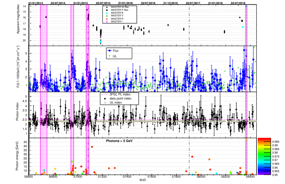
Figure 7: Light-curves, photon index and high-energy photons of NVSS J141922-083830 from 3 November 2013 to 28 November 2018 (MJD 56599 to 58450), encompassing the four flaring periods (highlighted with magenta shaded areas). The time stamp of the two SALT spectra are indicated by vertical grey dashed-dotted lines, and the time stamp of the MASTER-Net higher detected flux (7 September 2018 / MJD 58368.8545 at B=14.04) is indicated by a vertical green dashed line. Upper panel: MASTER-Net magnitudes from Figure 2. Second panel: Fermi-LAT light-curve in the 100 MeV–100 GeV energy range, for a three-day binning. Upper limits are shown in green. Third panel: power law photon index as optimised by the likelihood analysis for each bin of the Fermi-LAT light-curve. In light grey are indicated the values used for computing the upper limits (average values). Bottom panel: highest energy "ultraclean" photons candidates $>$ 5 GeV. The colour code labeled from 0.95 to 1.00 on the right indicates the probability for each event to be associated to NVSS J141922–083830.

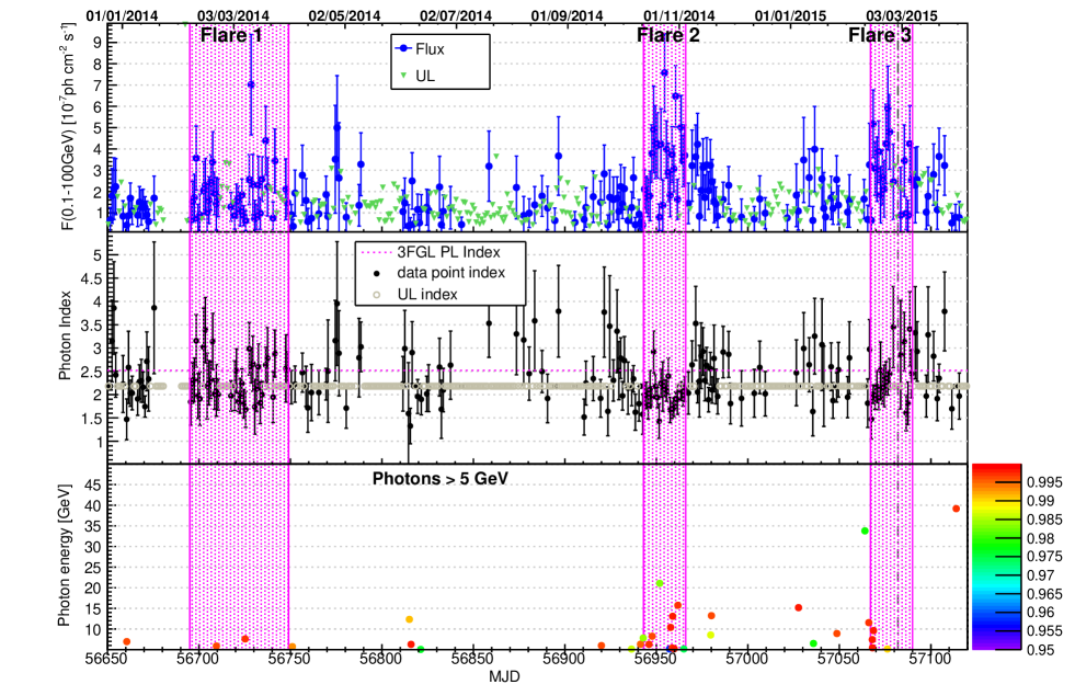
Figure 8: Fermi-LAT light-curve, photon index and high-energy photons of NVSS J141922-083830 from 24 December 2013 to 8 April 2015 (MJD 56650 to 57120), encompassing the first three flaring periods (highlighted with magenta shaded areas). The time stamp of the first SALT spectrum ($1^{st}$ March 2015) is indicated by a vertical grey dashed-dotted line. Upper panel: Fermi-LAT light-curve in the 100 MeV–100 GeV energy range, for a one-day binning. Upper limits are represented in green. Second panel: power law photon index as optimised by the likelihood analysis for each bin of the Fermi-LAT light-curve. In light grey are indicated the values used for computing the upper limits (average values). Bottom panel: highest energy "ultraclean" photons candidates $>$ 5 GeV. The colour code labeled from 0.95 to 1.00 on the right indicates the probability for each event to be associated to NVSS J141922–083830.

Swift performed six observations covering the interval 24 June 2013 (MJD 56468) to 4 March 2015 (MJD 57086), with details presented in Table 2. The X-ray data from XRT were reprocessed with the mission-specific heasoft tool xrtpipeline (version 0.13.4) with standard input parameters as recommended by the instrument team. This step generates new cleaned events files with the most recent calibrations. The events files thus generated are used in the multi-mission tool XSELECT for extracting source and background products. Four Swift observations of the NVSS J141922–083830 were performed in PC mode and two in WT mode. The source count rate was always $<$ 0.5 counts/s which confirms that the source is not affected by the pileup effect. A circular region of radius 75^", centred at ($\alpha$=14:19:22.560, $\delta$=-08:38:32.20) is used as source region. Whereas, for the background, two circular regions each of radius 150^" centered at ($\alpha$=14:19:27.57, $\delta$=-08:30:29.08) and ($\alpha$=14:19:57.636, $\delta$=-8:39:23.83) are used. We cross-checked for the presence of another X-ray source contaminating the source or background regions. The source being very faint, the two WT mode observations are not usable. Only the PC mode observations from OBSID 00046513007 are worth fitting the spectra and hence using for the X-ray part of the SED.

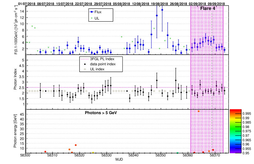
Figure 9: Fermi-LAT light-curve, photon index and high-energy photons of NVSS J141922-083830 from 1 July to 14 September 2018 (MJD 58300 to 58375), encompassing the fourth flaring period (highlighted with a magenta shaded area). The time stamp of the MASTER higher detected flux (7 September 2018 / MJD 58368.8545 at B=14.04) is indicated by a vertical green dashed line. Upper panel: Fermi-LAT light-curve in the 100 MeV–100 GeV energy range, for a one-day binning. Upper limits are represented in green. Second panel: power law photon index as optimised by the likelihood analysis for each bin of the Fermi-LAT light-curve. In light grey are indicated the values used for computing the upper limits (average values). Bottom panel: highest energy "ultraclean" photons candidates $>$ 5 GeV. The colour code labeled from 0.95 to 1.00 on the right indicates the probability for each event to be associated to NVSS J141922–083830.

4 Fermi-LAT observations and analysis

We collected data from NVSS J141922-083830 from the beginning of the Fermi-LAT mission until November 2018. We identified and studied four gamma-ray flares in the 2014–2018 period, labeled as "Flare 1", "Flare 2", "Flare 3" and "Flare 4" (Table 3). The MASTER-Net flares, that we reported in Section 2.1, were identified at the following dates:

• 16 May 2012 (MJD 56064);

• 24 March 2014 (MJD 56741, during "Flare 1");

• 21 February 2015 (MJD 57074.988, during "Flare 3");

• 15 July 2018 to 15 September 2018 (MJD 58315–58377, during "Flare 4").

We selected photons in the 100 MeV–100 GeV range. We used the Pass 8 (DR2) dataset (Atwood et al., 2013) and the software package — known as "Fermi Science Tools" (version v10r0p5). We selected “SOURCE” events within a 15^∘ radius region (region of interest — or ROI), centered at the position of NVSS J141922-083830. The “P8R2_SOURCE_V6” set of instrument response functions (IRFs) was used. Events which triggered the telescope with a zenith angle $\theta_{z}>90^{\circ}$ were removed in order to avoid contamination from the Earth limb radiation. The signal was extracted using an unbinned likelihood method, coded in the gtlike/pyLikelihood tool, part of the Fermi Science Tools. The Galactic diffuse emission and the isotropic backgrounds were modelled by the gll_iem_v06.fits and the iso_source_v06.txt templates, respectively, provided by the Fermi-LAT Collaboration. Since the likelihood analysis requires the fitting of the spectra of the sources within a certain distance of the source of interest, in order to re-associate each candidate photon of the ROI to its origin, we modelled all the point sources of the 3FGL (Acero et al., 2015) located in the ROI and in an additional surrounding 10^∘ wide annulus (called “Source Region”). In this model, spectral parameters were kept free (at least partially) for six point sources in the ROI, each one with a detection significance $>10\sigma$ in the 3FGL (four years of data). The normalisation parameters of both the isotropic and Galactic models were also kept free. NVSS J141922–083830 was modelled with a power law function for narrow time domain (light-curves) and narrow energy range (SED bins) analysis. (No extended source was found from the 3FGL in this region, apart the Galactic diffuse emission.)

Whenever the test statistics or the number of predicted counts of the source is below 3, for each time or spectral bin, an upper limit is plotted. We computed 95% confidence upper limits using the UpperLimits class from the Python version of the Fermi Science Tools, using the output of the actual unbinned likelihood analysis of the corresponding bin, having fixed the value of the power law spectral indices of the source of interest to their average value over periods similar to those displayed on the light-curves in Figures 7, 8 and 9.

The estimated systematic uncertainty in the effective area is 5% in the 100 MeV–100 GeV range. The energy resolution ($\Delta E/E$, at 68% containment) is 20% at 100 MeV, and between 6 and 10% over the 1–500 GeV range.

4.1 Light-curves in the 100 MeV–100 GeV range

We produced an 8-year (2008–2016) light-curve of the data we collected from NVSS J141922-083830 at the early stages of our work on this source, in order to search for significant gamma-ray outbursts, using a 3-day time binning. We identified three such events, now labeled as "Flare 1", "Flare 2" and "Flare 3", and also the long "Quiescent" period, all of which were mentioned earlier (see Table 3). Since the source was without significant gamma-ray flares for the first five years of the Fermi mission, we used this five-year period to represent the quiescent state of the source to which we compared its flux levels and the spectral shapes of the three outburst events. We reported part of this preliminary work in Britto et al. (2016).

After the detection of the main peak of "Flare 4" by MASTER-Net, we extended our data analysis up to the end of 2018. We present a three-day binned light-curve of the 2013–2018 period that encompasses the four flaring events in Figure 7. We chose a three-day binning as a compromise between getting enough statistically significant data points and a fair scanning of the time variability pattern of the source flux. The MASTER-Net optical light-curve is presented on the top panel (sub-range of Figure 2). On the second panel the Fermi-LAT light-curve is shown. The four flaring periods are highlighted with magenta shaded regions. Due to the scarce sampling in the optical, we did not perform correlation studies between both bands, but we can see that optical flares (whenever observations were possible) are coincident with gamma-ray flares within the highlighted range (Flares 1, 3 and 4).

In order to investigate the variability pattern of the source in more detail, we also produced one-day binned light-curves. We show these light-curves in the upper panels of Figure 8 (for Flares 1, 2 and 3) and Figure 9 (for Flare 4). In the middle panels are shown the spectral photon indices $\Gamma$. We note that the hardening of the spectrum is significant during parts of Flares 2, 3 and 4 (often with $\Gamma\lesssim 2$), when the source is brighter, which is a trend frequently observed for bright Fermi-LAT FSRQs and referred as the “harder when brighter” pattern. The value of $\Gamma$ becomes lower when the source is brighter. (We note a time gap during MJD 56681–56690 in Figures 8 and 9, as Fermi-LAT was mainly operating in pointing mode on other sky regions.)

Table 4: Spectral parameters obtained for NVSS J141922-083830 from the likelihood analysis of the Fermi-LAT data ($>$ 100 MeV). This is presented for the five periods mentioned in Table 3, when the source was modeled with a PL.

Phase	$N_{0}$	$\Gamma$	$E_{0}$	$N_{\rm pred}$	TS	F(E $>$ 100 MeV)	-ln(Likelihood)
	($10^{-12}$ cm-2 s-1 MeV-1)		(MeV)			(10-7 ph cm-2 s-1)
Quiescent	1.49 $\pm$ 0.10	2.28 $\pm$ 0.05	981.7	1936.2	441.3	0.21 $\pm$ 0.02	8672025.6
Flare 1	9.69 $\pm$ 0.88	2.30 $\pm$ 0.07	981.7	532.1	444.4	1.42 $\pm$ 0.14	344647.8
Flare 2	32.67 $\pm$ 2.28	1.98 $\pm$ 0.05	981.7	493.1	765.6	3.05 $\pm$ 0.26	180628.2
Flare 3	19.29 $\pm$ 2.11	2.18 $\pm$ 0.09	981.7	259.9	317.6	2.36 $\pm$ 0.29	102207.0
Flare 4	30.30 $\pm$ 2.77	2.13 $\pm$ 0.07	981.7	348.0	548.7	3.50 $\pm$ 0.34	84669.5

Table 5: Spectral parameters obtained for NVSS J141922-083830 from the likelihood analysis of the Fermi-LAT data ($>$ 100 MeV). This is presented for the five periods mentioned in Table 3, when the source was modeled with a LP.

Phase	$N_{0}$	$\alpha$	$\beta$	$E_{0}$	$N_{\rm pred}$	TS	F(E $>$ 100 MeV)	-ln(Likelihood)
	($10^{-12}$ cm-2 s-1 MeV-1)			(MeV)			(10-7 ph cm-2 s-1)
Quiescent	1.70 $\pm$ 0.13	2.27 $\pm$ 0.06	0.095 $\pm$ 0.042	981.7	1775.0	446.7	0.18 $\pm$ 0.02	8672022.3
Flare 1	10.43 $\pm$ 1.15	2.32 $\pm$ 0.08	0.058 $\pm$ 0.055	981.7	516.4	444.9	1.34 $\pm$ 0.16	344647.1
Flare 2	38.90 $\pm$ 3.38	1.94 $\pm$ 0.07	0.117 $\pm$ 0.043	981.7	460.3	772.7	2.63 $\pm$ 0.29	180623.4
Flare 3	19.30 $\pm$ 2.12	2.18 $\pm$ 0.09	$\sim 0$	981.7	260.0	317.5	2.37 $\pm$ 0.31	102207.0
Flare 4	32.62 $\pm$ 3.62	2.15 $\pm$ 0.08	0.051 $\pm$ 0.048	981.7	340.9	547.9	3.34 $\pm$ 0.37	84668.9

In the lower panels of Figures 7, 8 and 9 high energy (HE) photons ($>$ 5 GeV) are shown. These photons were obtained using the gtsrcprob tool, within a ROI=0.75^∘. This size of the ROI corresponds to the 68% containment angle of the acceptance weighted PSF at about 1.2 GeV. We used the ULTRACLEAN class of events, where counts have a higher probability to be real photons, compared to the source class events we used to obtain the light-curves and SEDs. The probability level shown on the figure corresponds to the probability that the candidate photons come from our source of interest. In the one-day binned light-curves, the probability levels of the high-energy photons may differ from those of Figure 7 as there were optimised by using the spectral parameters from the one-day binned likelihood analysis instead of the three-day one. HE photons were mainly observed during Flares 2, 3 and 4, as is often expected during flaring activities when the spectrum of the source becomes harder.

We determined the following highest gamma-ray fluxes of every flaring episode (one day averaged), respectively:

• on 12 Mar 2014 (MJD 56728): $(7.02\pm 2.36)\times 10^{-7}$ph cm^-2s^-1;

• on 24 Oct 2014 (MJD 56954): $(7.57\pm 1.83)\times 10^{-7}$ ph cm^-2s^-1;

• on 23 Feb 2015 (MJD 57076): $(5.92\pm 1.97)\times 10^{-7}$ ph cm^-2s^-1;

• on 5 Sep 2018 (MJD 58366): $(5.53\pm 1.33)\times 10^{-7}$ ph cm^-2s^-1.

(Higher fluxes preceding this latter flare, during MJD 58346–58353, could also be reported. However, the large error bars of these data points, that may indicate a low exposure, led us to discard these values – see Figure 9).

We also observed that the gamma-ray flux from NVSS J141922–083830 did not return down to that of the quiescent state during the long period in between Flare 2 and Flare 4 (from October 2014 to September 2018). Several minor episodes of activity occurred and were often accompanied by the emission of high-energy photons (Figure 7).

The highest energy photons detected were: at 33.8 GeV on 10 February 2015 (MJD 57063.9701, prob=0.9787) at the start/before Flare 3; at 39.2 GeV on 01 April 2015 (MJD 57113.8687, prob=0.9985), a few days after the end of Flare 3 and before a short secondary outburst; at 48.1 GeV on 2 September 2018 (MJD 58363.9374, prob=0.996243) at the beginning of Flare 4. (These probabilities prob cited above were calculated through the one-day binned likelihood analysis.) However, given the short duration of these flares and the limited statistics of high-energy photons, it remains difficult to establish a precise pattern on the arrival time of the photons during a flare.

We utilized the Gatspy implementation of the Lomb-Scargle method (VanderPlas & Ivezić, 2015) to derive a power spectrum of the 3-day binned Fermi-LAT light curve. No significant peaks were seen.

4.2 Time-resolved SEDs

Studies of the quiescent and flaring activities were also performed in the spectral domain, using the unbinned likelihood analysis. We first processed the analysis of each of the five periods (defined in Table 3), and obtained the spectral parameters of the best fit models, using both a power law (PL) and a log-parabolic (LP) function for NVSS J141922–083830 (Tables 4 and 5).

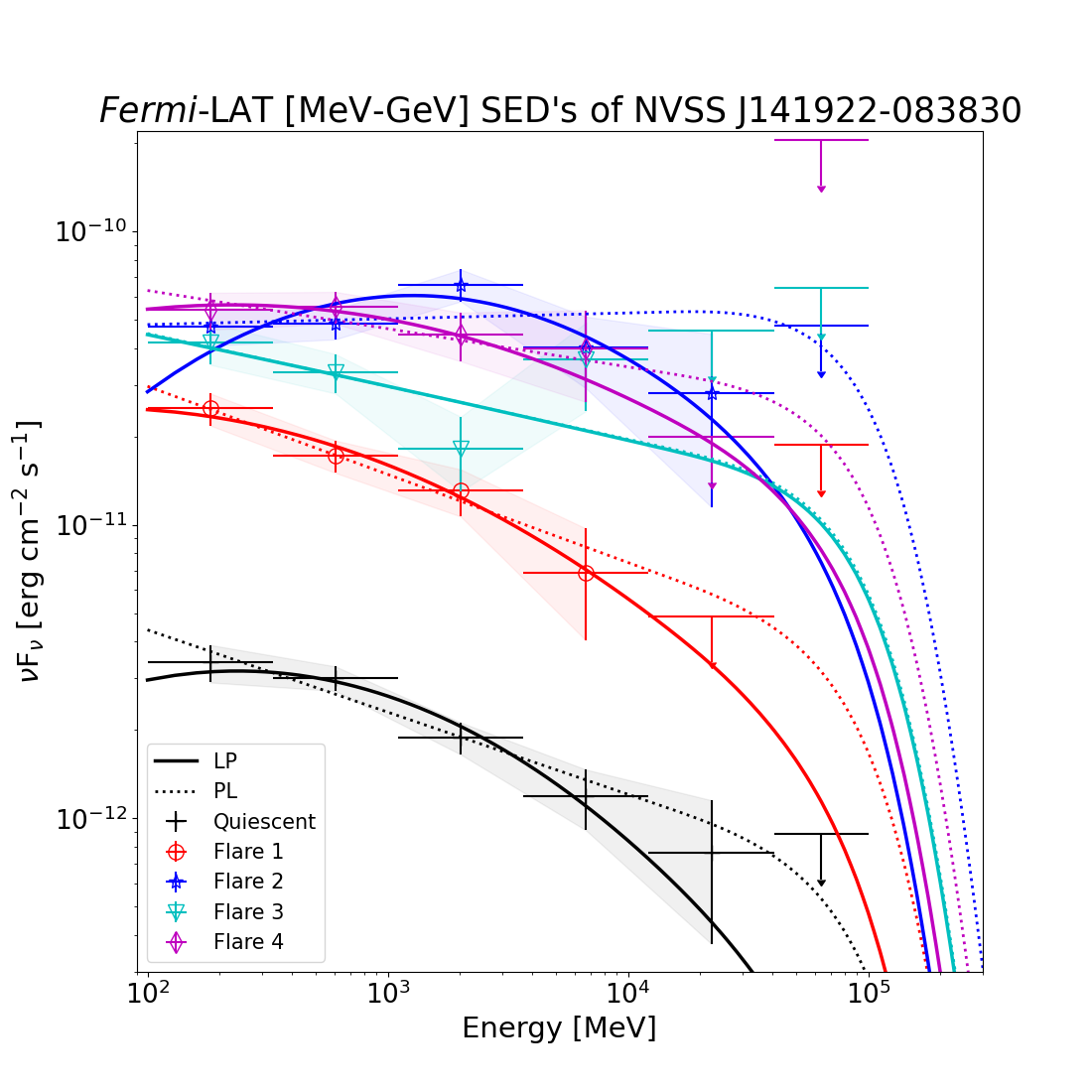
Figure 10: Fermi-LAT SEDs of NVSS J141922-083830, for the quiescent phase, Flare 1, Flare 2, Flare 3 and Flare 4, between 100 MeV and 100 GeV. The dotted and solid lines correspond to respectively the PL and LP fits of the data points, using the parameters obtained by the unbinned likelihood analysis as given in Table 4 and 5. The shaded areas were drawn from the uncertainties on the individual data points.

An optimised model for each period was used to compute an SED with six bins in energy in the 100 MeV–100 GeV energy range. After the optimisation of the spectral parameters over the whole energy range corresponding to each period (shown in Tables 4 and 5), each SED data point was obtained by running again the unbinned likelihood algorithm. This time, in addition to the previous model setup with a limited number of free parameters, we froze all spectral parameters that define the shape of the spectrum to their optimized values, even those of bright sources. The five SEDs are shown in Figure 10.

Flare 1 was significantly weaker than the others, Flares 2, 3 and 4 being at a similar flux level. Our results also show significant hardening during Flares 2 ($\Gamma\simeq 2.0$) and indications of hardening during Flares 3 and 4 ($\Gamma\simeq 2.0-2.1$), but not during Flare 1, where $\Gamma\simeq 2.3,$ as during the Quiescent phase (and in the 3FGL). This matches the "harder when brighter" trend which is often observed during major flares in FSRQs (Abdo et al., 2010a).

We fitted the SED data points by using both the PL and LP functions, whose parameters were computed through the unbinned likelihood analysis, respectively (Tables 4 and 5), and by adding the exponential factor $e^{-\tau(E)}$ to account for absorption by the extragalactic background light (EBL). The function $\tau(E)$ represents the EBL optical depth modelled by Finke et al. (2010), corresponding to a redshift z = 0.90. Hence we produced the fitted SEDs of Figure 10 by using the two following equations, respectively:

$$\left(\frac{dN}{dE}(E)\right)_{PL}=N_{0}\left(\frac{E}{E_{0}}\right)^{-\Gamma}e^{-\tau(E)};\hskip 39.83368pt$$ (1)

$$\left(\frac{dN}{dE}(E)\right)_{LP}=N_{0}\left(\frac{E}{E_{0}}\right)^{\alpha-\beta~{}ln(E/E_{0})}e^{-\tau(E)},$$ (2)

where $E_{0}$ = 981.713 MeV is the pivot energy of the NVSS J141922–083830 spectrum as reported in the 3FGL catalogue from the PL fit, and $\tau(E)$ is the opacity to the extragalactic background light. (Note: we needed to assume that the fit parameters found with the likelihood analysis – without EBL modelling – remained the best estimated ones even in the case where the factor $e^{-\tau(E)}$ is included in the fit functions. We do consider this approximation acceptable, since the departure from the PL fit is only observed from $\sim$20 GeV where the photon statistics is low.)

Table 6: Values of $TS_{\rm curv}$ computed with Equation 3 and values of $\chi^{2}/ndf$ for fitted data points, for the five observation periods.

		$\chi^{2}/ndf$ (data point fits)
Period	$TS_{\rm curv}$	————————————-
		$PLe^{-\tau(E)}$	$LPe^{-\tau(E)}$
Quiescent	6.5	0.19	0.17
Flare 1	1.3	0.080	0.082
Flare 2	9.6	1.39	0.42
Flare 3	0.0	0.86	0.86
Flare 4	1.2	0.21	0.11

We calculated the curvature spectrum significance by checking the compatibility of the LP function with the PL function, using:

$$TS_{\rm curv}=2\times[ln(\mathcal{L}_{LP})-ln(\mathcal{L}_{PL})],$$ (3)

where $ln(\mathcal{L}_{LP})$ and $ln(\mathcal{L}_{PL})$ are the natural logarithm of the maximum likelihood obtained with the LP and PL models, respectively, and reported in Tables 4 and 5. The curvature is considered to be significant if $TS_{\rm curv}\geq 4$ (Fermi-LAT Collaboration, 2022). Results are given in Table 6. Significant curvature is not observed for Phases 1, 3 and 4, but is observed for the Quiescent phase ($TS_{\rm curv}=6.5$) and Flare 2 ($TS_{\rm curv}=9.6$).

Fits on the binned SED data points allow for further investigation on the departure from either the PL or LP function. We find most of the computed $\chi^{2}/ndf$ values for each fit to be very small or $\lesssim 1.1$, except for the PL fit of Flare 2, where $\chi^{2}/ndf\simeq 1.4$. We also note a higher curvature during this flare compared to the quiescent state and the other flaring periods ($\beta=0.117\pm 0.043$ — see Table 5.)

Table 7: Gamma-ray isotropic luminosities during the five observation periods. These luminosities were derived using the integrated flux values in the 100 MeV–12 GeV range, found using a LP spectral fit (Equation 4.)

	Period	L (1047 erg s-1)
	Quiescent	0.5
$H_{0}$=67.4 k-1 Mpc-1	Flare 1	3.2
	Flare 2	10.2
$d_{L}$=19.570 Gly	Flare 3	6.2
	Flare 4	9.5
	Quiescent	0.4
$H_{0}$=73.2 km s-1 Mpc-1	Flare 1	2.7
	Flare 2	8.6
$d_{L}$=18.019 Gly	Flare 3	5.3
	Flare 4	8.1

4.3 Gamma-ray luminosities

Based on the redshift measurement reported in Section 2.2 (z = 0.903) and the results of the likelihood analysis presented in Table 5, we calculated the integrated apparent luminosity $L$ (isotropic assumption) of the source for the quiescent and flaring periods in the 100 MeV–12 GeV range, using the formula

$$L=4\pi d_{L}^{2}\int_{E_{1}}^{E_{2}}E\frac{dN(E)}{dE}dE,$$ (4)

where $E$, $E_{1}$ = 100 MeV and $E_{2}$ = 12 GeV are the energies in the observer frame, and $d_{L}$ is the luminosity distance (considering 1ly = $9.461.10^{26}$ cm).

We used the LP spectral shape. The choice of integrating up to 12 GeV was motivated by the fact that we do not get significant signal beyond this value in the SEDs. We use the cosmological parameters $\Omega_{m}$ = 0.315 and $\Omega_{\lambda}$ = 0.685 (Planck Collaboration et al., 2020). Due to the uncertainty on the measurement of the Hubble constant, we computed results with both $H_{0}$=67.4 (Planck Collaboration et al., 2020) and 73.2 km s^-1 Mpc^-1 (Riess et al., 2016). Results are given in Table 7.

5 Broad-band SED modeling

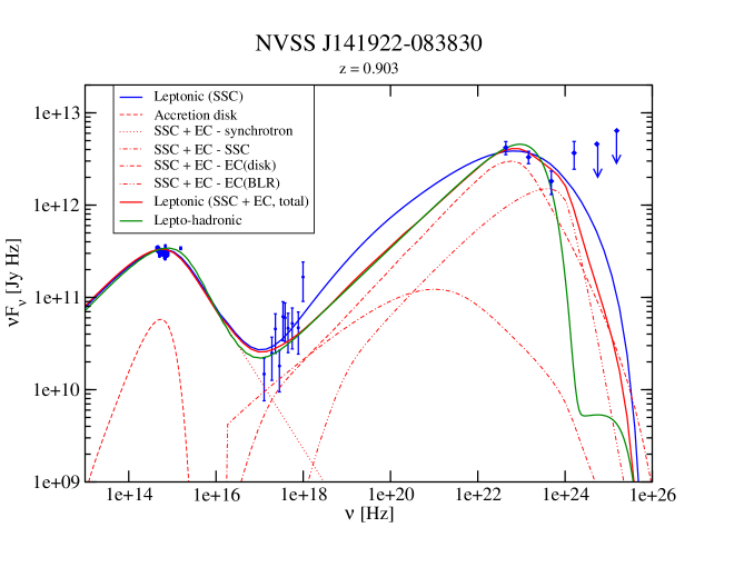
Figure 11: Multiwavelength SED of NVSS J141922–083830 during the February–March 2015 flare. Three steady-state single-zone model fits are presented: Blue: A leptonic model with only synchrotron and synchrotron-self-Compton emission; red: A leptonic model with also external-Compton emission included: dot-dashed = SSC, dot-dot-dashed = EC on direct accretion-disk photons; dot-dashed-dashed: EC on BLR emission; green: a lepto-hadronic model, where the $\gamma$-ray emission is dominated by proton synchrotron. See text and Table 8 for details and parameters, respectively.

Table 8: Model parameters for broad-band SED model fits.

Parameter	Leptonic SSC	Leptonic SSC + EC	Lepto-hadronic
Minimum electron injection $\gamma$	$1.1\times 10^{4}$	$1.3\times 10^{3}$	450
Maximum electron injection $\gamma$	$2.0\times 10^{5}$	$2.0\times 10^{5}$	$1.0\times 10^{4}$
Electron injection spectral index	3.5	3.5	4.0
Escape timescale parameter $\eta_{\rm esc}$	10	10	1
Magnetic field [G]	0.2	9	100
Radius of emission region [cm]	$2.5\times 10^{16}$	$1.5\times 10^{15}$	$1.0\times 10^{16}$
Bulk Lorentz factor $\Gamma_{\rm jet}$	10	20	20
Emission region distance from BH [pc]	—	0.028	—
Black-hole mass [M⊙]	—	$5\times 10^{9}$	—
Accretion-disk luminosity [erg s-1]	—	$1.0\times 10^{46}$	—
External radiation field T [K]	—	$4.0\times 10^{4}$	—
External radiation field u [erg cm-3]	—	$5.0\times 10^{-2}$	—
Minimum non-thermal proton energy [GeV]	—	—	1
Maximum non-thermal proton energy [GeV]	—	—	$2.8\times 10^{8}$
Proton injection spectral index	—	—	2.1
Kinetic luminosity in radiating electrons [erg s-1]	$2.8\times 10^{45}$	$2.5\times 10^{44}$	$2.6\times 10^{41}$
Poynting-flux luminosity [erg s-1]	$9.4\times 10^{42}$	$2.7\times 10^{44}$	$1.5\times 10^{48}$
Kinetic luminosity in radiating protons [erg s-1]	—	—	$1.9\times 10^{47}$
Magnetization $L_{B}/L_{e}$	$3.3\times 10^{-3}$	1.07	$5.8\times 10^{6}$
Magnetization $L_{B}/L_{p}$	—	—	7.8
Minimum variability time scale [h]	32	1.3	7.8

In order to provide further constraints on the classification of NVSS J141922–083830, we have compiled a quasi-simultaneous multi-wavelength SED around the time of the February–March 2015 flare (Flare 3), since this flare occuured at a time when the available multi-wavelength coverage was best. It includes NIR photometry from the CANICA/NIR camera of the 2.1m telescope of the Guillermo Haro Observatory (Carrasco et al., 2015), at MJD 57080.5378 (2015-02-27 12:54:25.920 UTC), Swift UVOT optical/near-UV photometry from the period during MJD 57070-57090, the Swift XRT X-ray spectrum from MJD 57085.1582 – 57085.2836 (2015-03-04) as well as the Fermi-LAT spectrum from the period MJD 57067 – 57090. The quasi-simultaneous SED is plotted in Figure 11. It shows the peak of the low-frequency SED component around optical wavelengths and the high-energy component peaking at sub-GeV energies, with a strong $\gamma$-ray dominance, the peak of the $\gamma$-ray component being about a factor 10 brighter than the low-frequency (synchrotron) component. These are SED features that are characteristic of LSP blazars, such as FSRQs and low-frequency-peaked BL Lac objects.

For illustrative purposes, we model this SED with the single-zone leptonic and lepto-hadronic models developed by Böttcher et al. (2013). These are steady-state models, which is justified for our purposes, since the data are not exactly simultaneous and the integration times for most of these observations are longer than the characteristic dynamical and radiative cooling time scales for electrons (and protons) emitting in the optical through $\gamma$-ray regimes.

The model is based on a single emission zone, assumed spherical in the co-moving frame, which is moving with Lorentz factor $\Gamma_{\rm jet}$ along the jet. A power-law energy distribution of electrons (and protons in the case of the lepto-hadronic model) is injected, and an equilibrium between injection, radiative (and adiabatic for protons in the lepto-hadronic model) energy losses, and escape from the emission region is calculated self-consistently to evaluate the final radiation spectrum. The particle escape time scale is parameterized as a multiple $\eta_{\rm esc}\geq 1$ of the light crossing time, such that $t_{\rm esc}=\eta_{\rm esc}\,R/c$, where $R$ is the radius of the emission region. Synchrotron emission, Compton scattering (both synchrotron self-Compton [SSC] and external Compton [EC]), and, for the lepto-hadronic model, photo-pair and photo-pion production are included. Internal $\gamma\gamma$ absorption and corresponding pair injection and cascading are also treated in a steady-state fashion, as detailed in Böttcher et al. (2013). The model SED includes the gamma-gamma absorption by the EBL, which is evaluated using the model of Finke et al. (2010) for the redshift of z = 0.903. In order to reduce the number of free parameters, the viewing angle is chosen as $\theta_{\rm obs}=1/\Gamma_{\rm jet}$. In the lepto-hadronic models, external photon fields (both for Compton scattering and for photo-hadronic processes) are not included.

As is obvious from Figure 11, the SED is not very well sampled, so there will be large parameter degeneracies in our fits. Our model fits are therefore not meant to provide meaningful constraints on the emission-region parameters, but just to illustrate that it is possible to represent the SED with standard one-zone emission scenarios. To illustrate this, we attempt three different fits: (1) the simplest possible leptonic model fit, including only synchrotron and SSC; (2) a leptonic model fit, including external radiation fields; and (3) a lepto-hadronic model. All 3 of these fits are shown in Figure 11, and the adopted relevant model parameters are listed in Table 8. We will discuss these three fits individually below.

(1) The pure SSC model is the one with the fewest free parameters. Thus, even while specific parameter values are still degenerate, in order not to over-shoot the observed X-ray spectrum, a very large minimum electron Lorentz factor is required. The large Compton dominance of the source along with the wide separation of the synchrotron and SSC peaks also requires a low magnetic field, leading to a strongly particle-dominated energy budget in the source, far away from equipartition. This is a common problem and one of the reasons why pure SSC models are generally dis-favoured for LSP blazars.

(2) A leptonic model including external radiation fields is capable of reproducing the SED of NVSS J141922–083830 with significantly more natural parameters, typical of FSRQs and many ISP blazars. In particular, model parameters can be chosen that correspond to equipartition between the kinetic energy in electrons and the magnetic field. In our model fit, the $\gamma$-ray emission is dominated by EC on direct disk emission, with sub-dominant contribution from EC on an isotropic (in the AGN rest frame) thermal radiation field with parameters that are appropriate to represent BLR emission (see Böttcher et al., 2013, for a discussion). Due to a very compact emission region, this model allows for sub-hour variability.

(3) Our fit using a lepto-hadronic model is based on strongly proton-synchrotron dominated high-energy emission. The relativistic electron population is energetically strongly sub-dominant. The energy carried along the jet is dominated by the strong magnetic field, as is typical for hadronic and lepto-hadronic models.

Based on SED considerations alone, we cannot claim a strong preference for either a leptonic SSC + EC model or a lepto-hadronic model.

6 Summary and conclusions

We have presented results of multi-wavelength observations of the blazar candidate NVSS J141922-083830, including optical photometry, polarimetry, and spectroscopy. Four large $\gamma$-ray flares were identified, with characteristic time scales of several days.

The optical spectra obtained with SALT-RSS showed two emission lines, identified as the Mg ii 2798Å and C iii] 1909Å lines, yielding a redshift of $z=0.903$ for the source.

Optical polarimetry revealed variable polarization at a level of $\Pi\sim 10$ %. This provides evidence for the synchrotron origin of the optical emission and further supports the blazar nature of this source. Given a characteristic optical spectral index of $\alpha\sim 1$, a perfectly ordered magnetic field in the optical emission region would lead to a degree of polarization of $\sim 75$ %. The significantly lower degree of polarization therefore indicates a partially ordered magnetic field.

We report a hardening of the gamma-ray spectrum during the last three flaring periods, with a power-law spectral index $\Gamma=2.0$–$2.1$, while the average flux was $\approx$ 3 $\times$ 10^-7 ph cm^-2s^-1. The maximum daily gamma-ray flux level was observed during MJD 56954 at $(7.57\pm 1.83)\times 10^{-7}$ ph cm^-2s^-1, during Flare 2.

The broad-band SED of NVSS J141922-083830 shows the characteristic double-bump structure with a low-frequency peak in the optical and a high-frequency peak at multi-MeV energies. These features, along with a Compton dominance factor of $\sim 10$ are characteristic of LSP blazars, such as FSRQs, although the synchrotron peak frequency of NVSS J141922-083830 appears to be located in the optical, which is more characteristic of an ISP blazar. However, there is some uncertainty on the position of the synchrotron peak due to the limited amount of data. A single-zone, leptonic model with an external radiation field characteristic of BLR radiation, is able to reproduce the SED with plausible parameters characteristic of FSRQs (e.g., Ghisellini et al., 2010; Böttcher et al., 2013) and equipartition between relativistic electrons and the magnetic field. Also a proton-synchrotron-dominated hadronic model can not be ruled out, but requires an extreme energy budget in excess of $10^{48}$ erg s^-1.

Data availability

The data underlying this article will be shared on reasonable request to the corresponding authors.

References

- Abdo et al. (2010a) Abdo A. A., et al., 2010a, ApJ, 710, 1271
- Abdo et al. (2010b) Abdo A. A., et al., 2010b, ApJ, 716, 30
- Abdollahi et al. (2020) Abdollahi S., et al., 2020, ApJS, 247, 33
- Acero et al. (2015) Acero F., et al., 2015, ApJS, 218, 23
- Ackermann et al. (2011) Ackermann M., et al., 2011, ApJ, 743, 171
- Ackermann et al. (2015) Ackermann M., et al., 2015, ApJ, 810, 14
- Ajello et al. (2020) Ajello M., et al., 2020, ApJ, 892, 105
- Atwood et al. (2009) Atwood W. B., et al., 2009, ApJ, 697, 1071
- Atwood et al. (2013) Atwood W., et al., 2013, arXiv e-prints, p. arXiv:1303.3514
- Ballet et al. (2020) Ballet J., Burnett T. H., Digel S. W., Lott B., 2020, arXiv e-prints, p. arXiv:2005.11208
- Böttcher et al. (2013) Böttcher M., Reimer A., Sweeney K., Prakash A., 2013, ApJ, 768, 54
- Bradley et al. (2019) Bradley L., et al., 2019, astropy/photutils: v0.7.1, doi:10.5281/zenodo.3478575
- Britto et al. (2016) Britto R. J., et al., 2016, in Reylé C., Richard J., Cambrésy L., Deleuil M., Pécontal E., Tresse L., Vauglin I., eds, SF2A-2016: Proceedings of the Annual meeting of the French Society of Astronomy and Astrophysics. pp 93–101
- Buckley et al. (2006) Buckley D. A. H., Swart G. P., Meiring J. G., 2006, in Society of Photo-Optical Instrumentation Engineers (SPIE) Conference Series. p. 62670Z, doi:10.1117/12.673750
- Buckley et al. (2015) Buckley D. A. H., Breytenbach J. B., Kniazev A., Kotze M. M., Potter S., Gorbovskoy E., Lipunov V., 2015, The Astronomer’s Telegram, 7167, 1
- Buckley et al. (2018) Buckley D. A. H., et al., 2018, MNRAS, 474, L71
- Burdanov et al. (2014) Burdanov A. Y., Krushinsky V. V., Popov A. A., 2014, Astrophysical Bulletin, 69, 368
- Burgh et al. (2003) Burgh E. B., Nordsieck K. H., Kobulnicky H. A., Williams T. B., O’Donoghue D., Smith M. P., Percival J. W., 2003, in Iye M., Moorwood A. F. M., eds, Society of Photo-Optical Instrumentation Engineers (SPIE) Conference Series Vol. 4841, Instrument Design and Performance for Optical/Infrared Ground-based Telescopes. pp 1463–1471, doi:10.1117/12.460312
- Cardelli et al. (1989) Cardelli J. A., Clayton G. C., Mathis J. S., 1989, ApJ, 345, 245
- Carpenter et al. (2015) Carpenter B., Becerra J., Ojha R., Pursimo T., 2015, The Astronomer’s Telegram, 7184, 1
- Carrasco et al. (2015) Carrasco L., Recillas E., Porras A., Leon-Tavares J., Chavushyan V., Carraminana A., 2015, The Astronomer’s Telegram, 7168, 1
- Chambers et al. (2016) Chambers K. C., et al., 2016, arXiv e-prints, p. arXiv:1612.05560
- Chiaro et al. (2016) Chiaro G., Salvetti D., La Mura G., Giroletti M., Thompson D. J., Bastieri D., 2016, MNRAS, 462, 3180
- Chiaro et al. (2018) Chiaro G., et al., 2018, arXiv e-prints, p. arXiv:1808.05881
- Condon et al. (1998) Condon J. J., Cotton W. D., Greisen E. W., Yin Q. F., Perley R. A., Taylor G. B., Broderick J. J., 1998, AJ, 115, 1693
- Crawford et al. (2010) Crawford S. M., et al., 2010, in Observatory Operations: Strategies, Processes, and Systems III. p. 773725, doi:10.1117/12.857000
- Cutri & et al. (2012) Cutri R. M., et al. 2012, VizieR Online Data Catalog, p. II/311
- D’Abrusco et al. (2014) D’Abrusco R., Massaro F., Paggi A., Smith H. A., Masetti N., Landoni M., Tosti G., 2014, ApJS, 215, 14
- Djorgovski et al. (2010) Djorgovski S. G., et al., 2010, The Astronomer’s Telegram, 2800, 1
- Drake et al. (2009) Drake A. J., et al., 2009, ApJ, 696, 870
- Fermi-LAT Collaboration (2022) Fermi-LAT Collaboration 2022, in preparation
- Finke et al. (2010) Finke J. D., Razzaque S., Dermer C. D., 2010, ApJ, 712, 238
- Ghisellini et al. (2010) Ghisellini G., Tavecchio F., Foschini L., Ghirlanda G., Maraschi L., Celotti A., 2010, MNRAS, 402, 497
- Gorbovskoy et al. (2013) Gorbovskoy E. S., et al., 2013, Astronomy Reports, 57, 233
- Gorbovskoy et al. (2016) Gorbovskoy E. S., et al., 2016, MNRAS, 455, 3312
- Kornilov et al. (2012) Kornilov V. G., et al., 2012, Experimental Astronomy, 33, 173
- Kostov & Bonev (2018) Kostov A., Bonev T., 2018, Bulgarian Astronomical Journal, 28, 3
- Lipunov et al. (2010) Lipunov V., et al., 2010, Advances in Astronomy, 2010, 349171
- Lipunov et al. (2015) Lipunov V., et al., 2015, The Astronomer’s Telegram, 7133, 1
- Lipunov et al. (2019a) Lipunov V. M., et al., 2019a, Astronomy Reports, 63, 293
- Lipunov et al. (2019b) Lipunov V. M., et al., 2019b, New Astron., 72, 42
- Lipunov et al. (2022) Lipunov V. M., et al., 2022, Universe, 8, 271
- Lott et al. (2020) Lott B., Gasparrini D., Ciprini S., 2020, arXiv e-prints, p. arXiv:2010.08406
- Monet et al. (2003) Monet D. G., et al., 2003, AJ, 125, 984
- Nolan et al. (2012) Nolan P. L., et al., 2012, ApJS, 199, 31
- Planck Collaboration et al. (2020) Planck Collaboration et al., 2020, A&A, 641, A6
- Riess et al. (2016) Riess A. G., et al., 2016, ApJ, 826, 56
- Schlafly & Finkbeiner (2011) Schlafly E. F., Finkbeiner D. P., 2011, ApJ, 737, 103
- Schlegel et al. (1998) Schlegel D. J., Finkbeiner D. P., Davis M., 1998, ApJ, 500, 525
- Urry & Padovani (1995) Urry C. M., Padovani P., 1995, PASP, 107, 803
- VanderPlas & Ivezić (2015) VanderPlas J. T., Ivezić Ž., 2015, ApJ, 812, 18