Sample Size Estimates for Risk-Neutral Semilinear PDE-Constrained Optimization

Abstract

The sample average approximation (SAA) approach is applied to risk-neutral optimization problems governed by semilinear elliptic partial differential equations with random inputs. After constructing a compact set that contains the SAA critical points, we derive nonasymptotic sample size estimates for SAA critical points using the covering number approach. Thereby, we derive upper bounds on the number of samples needed to obtain accurate critical points of the risk-neutral PDE-constrained optimization problem through SAA critical points. We quantify accuracy using expectation and exponential tail bounds. Numerical illustrations are presented.

90C15, 90C30, 90C60, 49J20, 49J55, 49K45, 49K20, 35J61

1 Introduction

Many objective functions of stochastic programs involve expectations of parameterized objective functions in one way or another. Large-scale stochastic programs arise in a multitude of applications, such as machine learning [46, 66], feedback stabilization of autonomous systems [45], statistical estimation [34, 65], and optimization of differential equations under uncertainty [61, 78]. When the parameter space is high-dimensional, these expectations cannot be accurately evaluated. A common approach to approximate such stochastic programs is the sample average approximation (SAA) method, yielding the SAA problem [38, 67, 70]. The SAA objective function is defined by the sample average of the parameterized objective function. The SAA approach has become popular in the literature on optimization under uncertainty with partial differential equations (PDEs) [33, 64, 78]. The key characteristic of the SAA approach as applied to risk-neutral PDE-constrained optimization is the fact that it yields PDE-constrained optimization problems which can be solved efficiently using existing, rapidly converging algorithms. While the SAA approach is easy to use, a central question is: how many samples are sufficient to obtain approximate critical points for the stochastic program via SAA critical points with high probability? An answer to this question also addresses the computational complexity of risk-neutral PDE-constrained optimization problems, as potentially expensive simulations of PDEs are required for each sample. In the present manuscript, we answer this question for a class of risk-neutral semilinear PDE-constrained optimization problems. Our analysis is inspired by those in [67, 70, 69].

We derive nonasymptotic sample size estimates for SAA critical points of infinite dimensional optimization problems governed by semilinear PDEs with random inputs. We consider the risk-neutral PDE-constrained optimization problem

(1) $$\min_{u\in L^{2}(D)}\,(1/2)\mathbb{E}[\|S(u,\xi)-y_{d}\|_{L^{2}(D)}^{2}]+(\alpha/2)\|u\|_{L^{2}(D)}^{2}+\psi(u),$$

where $\alpha>0$, $D\subset{}^{d}$ is a bounded Lipschitz domain, $y_{d}\in L^{2}(D)$, $L^{1}(D)$ $(L^{2}(D))$ is the Lebesgue space of (square) integrable functions defined on $D$, and $\xi$ is a random element mapping from a complete probability space to a complete probability space with sample space $\Xi$ being a complete, separable metric space. Moreover, for each $(u,\xi)\in L^{2}(D)\times\Xi$, $y=S(u,\xi)\in H_{0}^{1}(D)$ solves the state equation

(2) $$A(\xi)y+Q(y)=b(\xi)+B(\xi)u.$$

The Sobolev space $H_{0}^{1}(D)$ is formally introduced in Section 2. We state assumptions on the semilinear PDE (2) in Section 3. The function $\psi:L^{2}(D)\to(-\infty,\infty]$ in (1) is proper, convex and lower semicontinuous. An example for $\psi$ is given by $\psi(u)=\gamma\|u\|_{L^{1}(D)}$ if $u\in U_{0}$ and $\psi(u)=\infty$ otherwise, where $\gamma\geq 0$ and $U_{0}=\{\,u\in L^{2}(D)\colon\,\mathfrak{l}\leq u\leq\mathfrak{u}\,\}$ with $\mathfrak{l}$, $\mathfrak{u}\in L^{2}(D)$ and $\mathfrak{l}\leq\mathfrak{u}$. This function and its variants arise in control device placement applications such as tidal turbine layout optimization [19]. The SAA problem of (1) is given by

(3) $$\min_{u\in L^{2}(D)}\,\frac{1}{2N}\sum_{i=1}^{N}\|S(u,\xi^{i})-y_{d}\|_{L^{2}(D)}^{2}+(\alpha/2)\|u\|_{L^{2}(D)}^{2}+\psi(u),$$

where $\xi^{1}$, $\xi^{2},\ldots$ are independent identically distributed $\Xi$-valued random elements defined on a common complete probability space $(\Omega,\mathcal{F},P)$ and each $\xi^{i}$ has the same distribution as $\xi$. Here, $N\in\mathbb{N}$ is the sample size. Critical points of the SAA problem (3) can be efficiently computed using semismooth Newton methods [77, 71, 49].

The feasible set, $\{\,u\in L^{2}(D)\colon\,\psi(u)<\infty\,\}$, is generally non-compact. The lack of compactness and the nonconvexity of the risk-neutral PDE-constrained optimization problem (1) and its SAA problems complicate the derivation of sample size estimates, as these are typically derived using covering numbers of the feasible set [14, 37, 67, 70, 65]. Sample size estimates can be established for convex stochastic progams without the covering number approach [27, 66]. However, the risk-neutral PDE-constrained optimization problem (1) and its SAA problems are nonconvex. For deriving sample size estimates, our initial observation is that critical points of the SAA problem (3) are contained in a compact subset of the feasible set. To construct the compact set, we use optimality conditions, PDE stability estimates, and higher regularity of the reduced parameterized objective function’s gradient. Utilizing the covering numbers for Sobolev function classes established in [5, 6], we derive sample size estimates using arguments similar to those in [67, 70, 68, 69, 65, 14, 37, 51]. However, our focus is the analysis of SAA critical points as opposed to SAA solutions, as risk-neutral semilinear PDE-constrained optimization problems are nonconvex. For classes of risk-neutral linear elliptic PDE-constrained optimizations, SAA solutions are analyzed in [33, 50, 52, 53, 64]. However, the analysis in [53] does not generalize to nonconvex problems.

Alternative approximation approaches for risk-neutral PDE-constrained optimization problems include, for example, quasi-Monte Carlo sampling [28], low-rank tensor methods [4, 22], and stochastic collocation [8, 39, 73]. While we are unaware of a systematic theoretical and/or empirical study comparing, for example, Monte Carlo approaches, quasi-Monte Carlo sampling techniques, and sparse grid schemes as applied to risk-neutral nonconvex PDE-constrained optimization, we provide a brief comparision of these approaches in terms of characteristics used for their theoretical convergence anayses. Sparse grid-based discretizations may result in nonconvex optimization problems and their analysis requires smoothness properties with respect to the parameters and independent random variables with Lebesgue densities, but the methods in [40, 39, 79], which combine sparse grid techniques with trust-region schemes, perform very well. We refer the reader to [12] for the analysis of sparse grid-based approximations of finite dimensional stochastic programs. Monte Carlo sample-based approximations preserve convexity and only require mild integrability properties with respect to possibly infinitely many parameters, but are deemed to be quite slowly convergent. For finite dimensional stochastic programs, it is known that quasi-Monte Carlo methods can outperform Monte Carlo sampling techniques provided that the integrands satisfy certain regularity conditions [69, pp. 185–189]. The quasi-Monte Carlo approach is analyzed in [28] as applied to risk-neutral linear-quadratic control problems with PDEs, an important class of risk-neutral convex PDE-constrained optimization problems. As with every numerical scheme, each approximation approach for risk-neutral PDE-constrained optimization has its advantages and disadvantages. The Monte Carlo sample-based scheme is arguably the most widely used approach to approximating stochastic programs. This and the fact that it yields standard PDE-constrained optimization problems build our main motivation to establishing sample size estimates.

Outline of the paper

We discuss preliminaries and define further notation in Section 2. A class of risk-neutral semilinear PDE-constrained optimization problems is introduced in Section 3. PDE stability estimates are derived in section 3.1. In section 3.2, we compute the derivative of the expectation function and demonstrate the Lipschitz continuity of its gradient in section 3.3. The focus of our results in Section 3 is to make the PDE stability estimates’ dependence on problem-dependent parameters explicit. Section 3.4 discusses the existence of solutions. We combine the results established in Section 3 to construct a compact set containing the SAA critical points in Section 4. The covering numbers of Sobolev function classes used to establish nonasymptotic finite sample size estimates in Section 6 are provided in Section 5. In Section 8, we summarize our contributions, put our approach into perspective, and comment on potential improvements of our sample size estimates with respect to the dimension of the computational domain. In the appendices, we discuss auxiliary results used in Section 6 to derive the sample size estimates. Appendix A discusses the measurability of set inclusions and Appendix B provides sub-Gaussian-type expectation and tail bounds of maxima of Hilbert space-valued random vectors. The bounds are used in Appendix C to derive uniform expectation and exponential tail bounds for normal maps in Hilbert spaces. These bounds are applied in Section 6 for obtaining our nonasymptotic sample size estimates for SAA critical points.

2 Preliminaries and further notation

Relationships between random variables, vectors, and elements hold with probability one (w.p. $1$) if not specified otherwise. Metric spaces are equipped with their Borel $\sigma$-field. Let $X$, $X_{1}$ and $X_{2}$ be real Banach spaces. The space of bounded, linear operators from $X_{1}$ to $X_{2}$ is denoted by $\mathscr{L}(X_{1},X_{2})$. We define $X^{*}=\mathscr{L}(X,\real)$. The adjoint operator of $\Upsilon\in\mathscr{L}(X_{1},X_{2})$ is denoted by $\Upsilon^{*}\in\mathscr{L}(X_{2}^{*},X_{1}^{*})$. Throughout the text, $(\Theta,\mathcal{A},\mu)$ is a complete probability space. An operator-valued mapping $\Upsilon:\Theta\to\mathscr{L}(X_{1},X_{2})$ is called uniformly measurable if there exists a sequence of simple operators $\Upsilon_{k}:\Theta\to\mathscr{L}(X_{1},X_{2})$ such that $\Upsilon_{k}(\theta)$ converges to $\Upsilon(\theta)$ in $\mathscr{L}(X_{1},X_{2})$ as $k\to\infty$ for all $\theta\in\Theta$; cf. [30, Def. 3.5.5]. A function $\upsilon:\Theta\to X$ is strongly measurable if there exists a sequence of simple functions $\upsilon_{k}:\Theta\to X$ such that $\upsilon_{k}(\theta)\to\upsilon(\theta)$ as $k\to\infty$ for all $\theta\in\Theta$ [35, Def. 1.1.4]. If $X$ is separable, then $\upsilon:\Theta\to X$ is strongly measurable if and only if it is measurable [35, Cor. 1.1.2 and Thm. 1.1.6]. Let $\Gamma\colon\Theta\rightrightarrows X$ be a set-valued mapping with closed images. The mapping $\Gamma$ is called measurable if $\Gamma^{-1}(V)\in\mathcal{A}$ for each open set $V\subset X$ [2, Def. 8.1.1]. Here, $\Gamma^{-1}$ is the inverse image of $\Gamma$. An operator $\Upsilon\in\mathscr{L}(X_{1},X_{2})$ is compact if $\Upsilon(V)\subset X_{2}$ is precompact for each bounded set $V\subset X_{1}$. Let $Y$ be a complete metric space. A map $\Phi:Y\times\Theta\to X$ is a Carathéodory function if $\Phi(\cdot,\theta)$ is continuous for all $\theta\in\Theta$ and $\Phi(y,\cdot)$ is measurable for all $y\in Y$ [2, p. 311]. The Fréchet derivative of a mapping $h$ with respect to $y$ is denoted by $h_{y}$. For a real Hilbert space $H$, $(\cdot,\cdot)_{H}$ is its inner product and $\|h\|_{H}=(h,h)_{H}^{1/2}$ its norm. For a convex, lower semicontinuous, proper function $\varphi:H\to(-\infty,\infty]$, the proximity operator $\mathrm{prox}_{\varphi}:H\to H$ of $\varphi$ is defined by (see [3, Def. 12.23])

$$\mathrm{prox}_{\varphi}({v})=\operatorname*{arg\,min}_{w\in H}\,\varphi(w)+(1/2)\|v-w\|_{H}^{2}.$$

Throughout the text, $D\subset{}^{d}$ is a bounded Lipschitz domain. The space $L^{2}(D)$ is identified with its dual. The Sobolev space $H^{1}(D)$ is defined by all $L^{2}(D)$-functions with square integrable weak derivatives and $H_{0}^{1}(D)$ consists all $v\in H^{1}(D)$ with zero boundary traces. We define $H^{-1}(D)=H_{0}^{1}(D)^{*}$. The dual pairing between $H^{-1}(D)$ and $H_{0}^{1}(D)$ is denoted by $\langle\cdot,\cdot\rangle_{H^{-1}(D),H_{0}^{1}(D)}$. We equip $H_{0}^{1}(D)$ with $\|v\|_{H_{0}^{1}(D)}=\|\|\nabla v\|_{2}\|_{L^{2}(D)}$ and $H^{1}(D)$ with $\|v\|_{H^{1}(D)}=(\|v\|_{L^{2}(D)}^{2}+\|v\|_{H_{0}^{1}(D)}^{2})^{1/2}$. Here, $\nabla v$ is the weak gradient of $v$ and $\|\cdot\|_{2}$ is the Euclidean norm on ^d. Throughout the text, $\iota:H_{0}^{1}(D)\to L^{2}(D)$ given by $\iota v=v$ is the embedding operator of the compact embedding $H_{0}^{1}(D)\xhookrightarrow{}L^{2}(D)$ and $C_{D}$ is Friedrichs’ constant, the operator norm of $\iota$. We have $C_{D}=\|\iota^{*}\|_{\mathscr{L}(L^{2}(D),H^{-1}(D))}$. We denote by $|D|$ the Lebesgue measure of $D$ and by $\bar{D}$ its closure. We define $C^{0,1}(\bar{D})$ as the space of Lipschitz continuous real-valued functions defined on $\bar{D}$ and equip it with the usual norm $\|\cdot\|_{C^{0,1}(\bar{D})}$ defined in [32, p. 16].

Let $(X,\|\cdot\|_{X})$ be a normed space, let $X_{0}\subset X$ be nonempty and totally bounded, and let $\nu>0$. The $\nu$-covering number $\mathcal{N}(\nu;X_{0},\|\cdot\|_{X})$ is the minimal number of closed $\|\cdot\|_{X}$-balls with radius $\nu$ in $X$ needed to cover $X_{0}$ (cf. [74, pp. 87–88]). This notion of covering numbers does not require the centers of the $\|\cdot\|_{X}$-balls be contained in $X_{0}$.

3 Risk-neutral semilinear PDE-constrained optimization

We impose conditions on the parameterized PDE (2) which ensure the existence and uniqueness of solutions. These conditions ensure that the semilinear PDE (2) is a monotone operator equation and hence the existence of solutions and the stability estimates can be established using the Minty–Browder theorem [80, Thm. 26.A], for example. Semilinear PDE-constrained optimization problems are analyzed, for example, in [23, 25, 43, 75, 77]. In this section, our contributions are to address some measurability questions, and to derive stability estimates and a bound on an objective function’s Lipschitz constant with the dependence on problem data’s characteristics made explicit. Even though our derivations are built on standard techniques, the stability estimates are needed for establishing our nonasymptotic sample size estimates (see Section 6).

We define $F:L^{2}(D)\to\real$ and $\hat{F}_{N}:L^{2}(D)\to\real$ by

(4) $$F(u)=(1/2)\mathbb{E}[\|\iota S(u,\xi)-y_{d}\|_{L^{2}(D)}^{2}]\quad\text{and}\quad\hat{F}_{N}(u)=\frac{1}{2N}\sum_{i=1}^{N}\|\iota S(u,\xi^{i})-y_{d}\|_{L^{2}(D)}^{2}.$$

As opposed to the problem formulations in (1) and (3), we make here the use of the embedding operator $\iota$ explicit. Since the random elements $\xi^{1},\xi^{2},\ldots$ are defined on the complete probability space $(\Omega,\mathcal{F},P)$, we can view $\hat{F}_{N}$ as a function defined on $L^{2}(D)\times\Omega$. However, we often omit the second argument.

We define the feasible set $U_{\text{ad}}=\{\,u\in L^{2}(D)\colon\,\psi(u)<\infty\,\}$. [Control regularization and feasible set]

1. The function $\psi:L^{2}(D)\to(-\infty,\infty]$ is proper, convex and lower semicontinuous.

2. For some $r_{\text{ad}}\in(0,\infty)$, $\|u\|_{L^{2}(D)}\leq r_{\text{ad}}$ for all $u\in U_{\text{ad}}$.

3.1 Semilinear PDEs with random inputs

We impose conditions on the data defining the semilinear PDE (2) based on those used in [43, Assumptions (3.1)–(3.3)], [77, sect. 9.1], and [23, Assumption 2.2].

[Semilinear PDE: Problem data]

1. $D\subset{}^{d}$ is a bounded Lipschitz domain with $d\in\{2,3\}$.

2. $A:\Xi\to\mathscr{L}(H_{0}^{1}(D),H^{-1}(D))$ is uniformly measurable. There exists a constant $\kappa_{\min}>0$ such that $A(\xi)$ is self-adjoint and $\langle A(\xi)y,y\rangle_{H^{-1}(D),H_{0}^{1}(D)}\geq\kappa_{\min}\|y\|_{H_{0}^{1}(D)}^{2}$ for all $y\in H_{0}^{1}(D)$ and each $\xi\in\Xi$.

3. $b:\Xi\to H^{-1}(D)$ and $g:\Xi\to C^{0,1}(\bar{D})$ are strongly measurable and there exist constants $b_{\max}$, $g_{\max}>0$ such that $\|b(\xi)\|_{H^{-1}(D)}\leq b_{\max}$ and $\|g(\xi)\|_{C^{0,1}(\bar{D})}\leq g_{\max}$ for each $\xi\in\Xi$.

4. For each $\xi\in\Xi$, $B(\xi)\in\mathscr{L}(L^{2}(D),H^{-1}(D))$ is defined by

   (5) $$\langle B(\xi)u,v\rangle_{H^{-1}(D),H_{0}^{1}(D)}=(g(\xi)u,v)_{L^{2}(D)}.$$

5. We define $Q:H_{0}^{1}(D)\to H^{-1}(D)$ by $\langle Q(y),v\rangle_{H^{-1}(D),H_{0}^{1}(D)}=(q(y),v)_{L^{2}(D)}$. The function $q:\real\to\real$ is nondecreasing, twice continuously differentiable, $q(0)=0$, and $|q^{\prime\prime}(t)|\leq c_{q}+d_{q}|t|^{p-3}$ for all $t\in\real$, where $c_{q}$, $d_{q}\geq 0$ and $p\in(3,\infty)$ if $d=2$ and $p\in(3,6]$ if $d=3$.

 (a) and  (e) ensure that the embedding $H_{0}^{1}(D)\xhookrightarrow{}L^{p}(D)$ is continuous [32, Thm. 1.14] and that $q$ is twice continuously differentiable as a superposition operator from $L^{p}(D)$ to $L^{p^{*}}(D)$ [77, p. 202], where $p^{*}\in[1,\infty)$ fulfills $1/p+1/p^{*}=1$. Hence, $Q$ is twice continuously differentiable from $H_{0}^{1}(D)$ to $H^{-1}(D)$. Moreover $Q$ is monotone. Hence Section 3.1 ensures that for each $\xi\in\Xi$, the operator $H_{0}^{1}(D)\ni y\mapsto A(\xi)y+Q(y)\in H^{-1}(D)$ is continuous and strongly monotone with parameter $\kappa_{\min}$ and hence coercive [80, p. 501]. We denote by $c_{p}>0$ the embedding constant of the embedding $H_{0}^{1}(D)\xhookrightarrow{}L^{p}(D)$. Under  (a) and  (e), the constant $c_{p}$ is finite since $d\in\{2,3\}$ and $p\in[1,6]$ [32, Thm. 1.14]. Lemma 3.1 establishes basic properties of the mapping $B$. In particular, we establish its uniform measurability and some of its compactness properties.

Lemma 3.1.

If  (a),  (c), and  (d) hold, then for all $\xi\in\Xi$,

1. $B:\Xi\to\mathscr{L}(L^{2}(D),H^{-1}(D))$ is uniformly measurable and

   $$\|B(\xi)\|_{\mathscr{L}(L^{2}(D),H^{-1}(D))}\leq C_{D}\|g(\xi)\|_{C^{0,1}(\bar{D})},$$

2. $B(\xi)^{*}v=\iota[g(\xi)v]=g(\xi)v$ for all $v\in H_{0}^{1}(D)$, and $B(\xi)^{*}$ and $B(\xi)$ are compact.

We prove Lemma 3.1 using Lemma 3.2. Lemma 3.2 establishes an explicit continuity constant of a certain bilinear mapping in terms of Friedrichs’ constant.

Lemma 3.2.

Let $D\subset{}^{d}$ be a bounded Lipschitz domain. If $v\in C^{0,1}(\bar{D})$ and $w\in H_{0}^{1}(D)$, then $vw\in H_{0}^{1}(D)$ and $\|vw\|_{H_{0}^{1}(D)}\leq(C_{D}+1)\|v\|_{C^{0,1}(\bar{D})}\|w\|_{H_{0}^{1}(D)}$.

Proof 3.3.

Using [26, Thm. 1.4.1.2], we have $vw\in H_{0}^{1}(D)$. Since $v$ is Lipschitz continuous, we have $\|\|\nabla v\|_{2}\|_{L^{\infty}(D)}\leq\|v\|_{C^{0,1}(\bar{D})}$. Using $\nabla[vw]=w\nabla v+v\nabla w$ and the Hölder inequality, we obtain $\|vw\|_{H_{0}^{1}(D)}\leq\|v\|_{C^{0,1}(\bar{D})}(\|w\|_{L^{2}(D)}+\|\|\nabla w\|_{2}\|_{L^{2}(D)})$. Combined with Friedrichs’ inequality, we obtain the stability estimate.

Proof 3.4 (Proof of Lemma 3.1).

Let us fix $u\in L^{2}(D)$, $v\in H_{0}^{1}(D)$, and $\xi\in\Xi$.

1. We define $\varrho:C^{0,1}(\bar{D})\to\mathscr{L}(L^{2}(D),H^{-1}(D))$ by $\langle\varrho(g)u,v\rangle_{H^{-1}(D),H_{0}^{1}(D)}=(gu,v)_{L^{2}(D)}$. The map $\varrho$ is Lipschitz continuous with Lipschitz constant $C_{D}$. Combined with $B=\varrho\circ g$ (see (5)) and the strong measurability of $g$, we find that $B$ is uniformly measurable [35, Cor. 1.1.11]. The bound on the operator norm of $B(\xi)$ is implied by the above Lipschitz continuity.

2. We have $(B(\xi)^{*}v,u)_{L^{2}(D)}=(g(\xi)v,u)_{L^{2}(D)}$ for all $u\in L^{2}(D)$. Since $g(\xi)\in C^{0,1}(\bar{D})$, $g(\xi)v\in H_{0}^{1}(D)$ [26, Thm. 1.4.1.2]. Hence, $B(\xi)^{*}v=\iota[g(\xi)v]$. The map $H_{0}^{1}(D)\ni v\mapsto g(\xi)v\in H_{0}^{1}(D)$ is linear and bounded (see Lemma 3.2). Hence $B(\xi)^{*}$ is compact. Now Schauder’s theorem [13, Thm. 3.4 on p. 174] implies that $B(\xi)$ is compact.

The next lemma is essentially known; cf. [77, 43, 23].

Lemma 3.5.

Let Section 3.1 hold. For each $(u,\xi)\in L^{2}(D)\times\Xi$, the parameterized PDE (2) has a unique solution $S(u,\xi)\in H_{0}^{1}(D)$ and

(6) $$\|S(u,\xi)\|_{H_{0}^{1}(D)}\leq(1/\kappa_{\min})\|b(\xi)\|_{H^{-1}(D)}+(C_{D}/\kappa_{\min})\|g(\xi)\|_{C^{0,1}(\bar{D})}\|u\|_{L^{2}(D)}.$$

Moreover, for each $(u_{1},u_{2},\xi)\in L^{2}(D)^{2}\times\Xi$,

(7) $$\|S(u_{2},\xi)-S(u_{1},\xi)\|_{H_{0}^{1}(D)}\leq(C_{D}/\kappa_{\min})\|g(\xi)\|_{C^{0,1}(\bar{D})}\|u_{2}-u_{1}\|_{L^{2}(D)}.$$

Proof 3.6.

The existence and uniqueness is implied by [80, Thm. 26.A]. We have $\kappa_{\min}\|S(u,\xi)\|_{H_{0}^{1}(D)}\leq\|b(\xi)+B(\xi)u\|_{H^{-1}(D)}$ (cf. [43, eq. (3.5)]) and

(8) $$\kappa_{\min}\|S(u_{2},\xi)-S(u_{1},\xi)\|_{H_{0}^{1}(D)}\leq\|B(\xi)[u_{2}-u_{1}]\|_{H^{-1}(D)};$$

cf. [80, p. 560] and [43, eq. (3.5)]. Combined with Lemma 3.1, we obtain (6) and (7).

3.2 Derivative computation

We show that the functions $F$ and $\hat{F}_{N}$ are Fréchet differentiable, compute their derivatives using the adjoint approach, and derive further stability estimates. The derivative formulas and the stability estimates are crucial for obtaining our finite sample size estimates.

Let us define $J:L^{2}(D)\times\Xi\to\real$ by

(9) $$J(u,\xi)=(1/2)\|\iota S(u,\xi)-y_{d}\|_{L^{2}(D)}^{2}.$$

For each $(u,\xi)\in L^{2}(D)\times\Xi$, $z=z(u,\xi)\in H_{0}^{1}(D)$ solves the adjoint equation

(10) $$[A(\xi)+Q_{y}(S(u,\xi))]z=-\iota^{*}[\iota S(u,\xi)-y_{d}].$$

To derive (10), we have used the fact that $A(\xi)$ (see  (b)) and $Q_{y}(y)$ are self-adjoint for each $(y,\xi)\in H_{0}^{1}(D)\times\Xi$ (cf. [23, eq. (2.8)]).

Proposition 3.7.

If Section 3.1 holds, then $F$ and $\hat{F}_{N}$ defined in (4) are Fréchet differentiable. For each $u\in L^{2}(D)$, it holds that $\nabla F(u)$, $\nabla\hat{F}_{N}(u)\in H_{0}^{1}(D)$,

(11) $$\nabla F(u)=-\mathbb{E}[g(\xi)z(u,\xi)]\quad\text{and}\quad\nabla\hat{F}_{N}(u)=-\frac{1}{N}\sum_{i=1}^{N}g(\xi^{i})z(u,\xi^{i}).$$

The proof of Proposition 3.7 uses Lemmas 3.8 and 3.10.

Lemma 3.8.

If Section 3.1 holds, then the following statements hold.

1. For each $(u,\xi)\in L^{2}(D)\times\Xi$, the adjoint equation (10) has a unique solution $z(u,\xi)\in H_{0}^{1}(D)$ and

   (12) $$\begin{aligned} \|z(u,\xi)\|_{H_{0}^{1}(D)}&\leq(C_{D}/\kappa_{\min})\|\iota S(u,\xi)-y_{d}\|_{L^{2}(D)}.\end{aligned}$$

2. The solution operator $S:L^{2}(D)\times\Xi\to H_{0}^{1}(D)$ is a Carathéodory mapping.

3. If $s:\Xi\to H_{0}^{1}(D)$ is measurable, then $\Xi\ni\xi\mapsto Q_{y}(s(\xi))\in\mathscr{L}(H_{0}^{1}(D),H^{-1}(D))$ is uniformly measurable.

4. The adjoint state $z:L^{2}(D)\times\Xi\to H_{0}^{1}(D)$ is a Carathéodory function.

5. $L^{2}(D)\times\Xi\ni(u,\xi)\mapsto g(\xi)z(u,\xi)\in H_{0}^{1}(D)$ is a Carathéodory map. For each $u\in L^{2}(D)$, $\Xi\ni\xi\mapsto g(\xi)z(u,\xi)\in H_{0}^{1}(D)$ is Bochner integrable and

   (13) $$\|g(\xi)z(u,\xi)\|_{H_{0}^{1}(D)} \leq(C_{D}+1)\|g(\xi)\|_{C^{0,1}(\bar{D})}\|z(u,\xi)\|_{H_{0}^{1}(D)}.$$

Proof 3.9.

1. The assertions are a consequence of the Lax–Milgram lemma and the fact that $C_{D}=\|\iota^{*}\|_{\mathscr{L}(L^{2}(D),H^{-1}(D))}$.

2. Let us define the nonlinear operator $E:H_{0}^{1}(D)\times L^{2}(D)\times\Xi\to H^{-1}(D)$ by $E(y,u,\xi)=A(\xi)y+Q(y)-b(\xi)-B(\xi)u$. Then $S(u,\xi)$ solves (2) if and only if $E(S(u,\xi),u,\xi)=0$. As in the proofs of [77, Lems. 9.2 and 9.6], we can show that $E(\cdot,\cdot,\xi)$ is twice continuously differentiable for each $\xi\in\Xi$ and that $\langle E_{y}(y,u,\xi)v,v\rangle_{H^{-1}(D),H_{0}^{1}(D)}\geq\kappa_{\min}\|v\|_{H_{0}^{1}(D)}^{2}$ for each $(y,v,u,\xi)\in H_{0}^{1}(D)^{2}\times L^{2}(D)\times\Xi$. Hence, the implicit function theorem and the Lax–Milgram lemma [32, Lem. 1.8] ensure that $S(\cdot,\xi)$ is twice continuously differentiable for each $\xi\in\Xi$. For each $u\in L^{2}(D)$, the measurability of $S(u,\cdot)$ is implied by the proof of [20, Thm. 3.12].

3. Since $H_{0}^{1}(D)\ni y\mapsto Q_{y}(y)\in\mathscr{L}(H_{0}^{1}(D),H^{-1}(D))$ is continuous and $s$ is strongly measurable, $Q_{y}\circ s$ is uniformly measurable [35, Cor. 1.1.11].

4. For each $y\in H_{0}^{1}(D)$, $v\mapsto Q_{y}(y)v$ is monotone. Hence, for each $\xi\in\Xi$, $\langle A(\xi)y+Q_{y}(S(u,\xi))y,y\rangle_{H^{-1}(D),H_{0}^{1}(D)}\geq\kappa_{\min}\|y\|_{H_{0}^{1}(D)}^{2}$ for all $y\in H_{0}^{1}(D)$. Now, the implicit function theorem and part (b) can be used to deduce the twice continuous differentiability of $z(\cdot,\xi)$ for all $\xi\in\Xi$. Fix $u\in L^{2}(D)$. Section 3.1, and parts (b) and (c) ensure that $\Xi\ni\xi\mapsto A(\xi)+Q_{y}(S(u,\xi))$ is uniformly measurable. The measurability of $z(u,\cdot)$ is now implied by part (b) when applied to the adjoint equation (10) rather than the state equation (2).

5. For each $\xi\in\Xi$, part (d) and Lemma 3.2 ensure the continuity of $L^{2}(D)\ni u\mapsto g(\xi)z(u,\xi)\in H_{0}^{1}(D)$. Now, let $u\in L^{2}(D)$. Let us define $\varrho_{1}:\Xi\to C^{0,1}(\bar{D})\times H_{0}^{1}(D)$ by $\varrho_{1}(\xi)=(g(\xi),z(u,\xi))$. Since $g$ and $z(u,\cdot)$ are strongly measurable (see part (d)), $\varrho_{1}$ is strongly measurable. We also define $\varrho_{2}:C^{0,1}(\bar{D})\times H_{0}^{1}(D)\to H_{0}^{1}(D)$ by $\varrho_{2}(g,z)=gz$. Lemma 3.2 ensures that $\varrho_{2}$ is bounded. Combined with the fact that $\varrho_{2}$ is bilinear, we find that $\varrho_{2}$ is continuous. We have $g(\xi)z(u,\xi)=(\varrho_{2}\circ\varrho_{1})(\xi)$ for all $\xi\in\Xi$. Thus, the chain rule [35, Cor. 1.1.11] ensures the measurability of $\Xi\ni\xi\mapsto g(\xi)z(u,\xi)\in H_{0}^{1}(D)$.

   Lemma 3.2 yields (13). Using (6), (12), (13),  (c), and the measurability of $\Xi\ni\xi\mapsto g(\xi)z(u,\xi)\in H_{0}^{1}(D)$, we have $\mathbb{E}[\|g(\xi)z(u,\xi)\|_{H_{0}^{1}(D)}]<\infty$. Hence, $\Xi\ni\xi\mapsto g(\xi)z(u,\xi)\in H_{0}^{1}(D)$ is Bochner integrable [35, Prop. 1.2.2].

Lemma 3.10 establishes bounds on the gradient of $J$.

Lemma 3.10.

If Section 3.1 holds, then $J(\cdot,\xi)$ is twice continuously differentiable for all $\xi\in\Xi$. For all $(u,\xi)\in L^{2}(D)\times\Xi$, $\nabla_{u}J(u,\xi)=-g(\xi)z(u,\xi)$ and

(14) $$\|\nabla_{u}J(u,\xi)\|_{H_{0}^{1}(D)} \leq(C_{D}+1)(C_{D}/\kappa_{\min})\|g(\xi)\|_{C^{0,1}(\bar{D})}\big{(}(C_{D}/\kappa_{\min})\|b(\xi)\|_{H^{-1}(D)}+$$

$$\quad\quad(C_{D}^{2}/\kappa_{\min})\|g(\xi)\|_{C^{0,1}(\bar{D})}\|u\|_{L^{2}(D)}+\|y_{d}\|_{L^{2}(D)}\big{)},$$

(15) $$\|\nabla_{u}J(u,\xi)\|_{L^{2}(D)} \leq(C_{D}^{2}/\kappa_{\min})\|g(\xi)\|_{C^{0,1}(\bar{D})}\big{(}C_{D}\|S(u,\xi)\|_{H_{0}^{1}(D)}+\|y_{d}\|_{L^{2}(D)}\big{)}.$$

Proof 3.11.

Adapting the proof of [77, Lem. 9.8], we obtain that $J(\cdot,\xi)$ is twice continuously differentiable on $L^{2}(D)$ with $\nabla_{u}J(u,\xi)=-g(\xi)z(u,\xi)$ for each $(u,\xi)\in L^{2}(D)$. Combined with (12) and (13), we obtain

$$\|\nabla_{u}J(u,\xi)\|_{H_{0}^{1}(D)}\leq(C_{D}+1)(C_{D}/\kappa_{\min})\|g(\xi)\|_{C^{0,1}(\bar{D})}\|\iota S(u,\xi)-y_{d}\|_{L^{2}(D)}.$$

Together with (6), we obtain (14). Using (12) and Friedrichs’ inequality, we have

$$\|\nabla_{u}J(u,\xi)\|_{L^{2}(D)}\leq\|g(\xi)z(u,\xi)\|_{L^{2}(D)}\leq\tfrac{C_{D}^{2}}{\kappa_{\min}}\|g(\xi)\|_{C^{0,1}(\bar{D})}\|\iota S(u,\xi)-y_{d}\|_{L^{2}(D)}.$$

Hence, we obtain (15).

Proof 3.12 (Proof of Proposition 3.7).

Combining the stability estimates (6) and (14), and Friedrichs’ inequality, we can apply [25, Lem. C.3] to deduce the Fréchet differentiability of $F$ and of $\hat{F}_{N}$ and the formulas in (11). Owing to (11) and Lemma 3.8, we find that $\nabla F(u)$, $\nabla\hat{F}_{N}(u)\in H_{0}^{1}(D)$.

3.3 Lipschitz constant computation

We compute a deterministic Lipschitz constant of the gradient $\nabla_{u}J(\cdot,\xi)$ on $U_{\text{ad}}$ for $\xi\in\Xi$.

Proposition 3.13.

If Sections 3.1 and  (b) hold, then for each $\xi\in\Xi$, the map $\nabla_{u}J(\cdot,\xi)$ is Lipschitz continuous on $U_{\text{ad}}$ with Lipschitz constant $L_{\nabla J}$ given by

$$L_{\nabla J} =C_{D}g_{\max}\bigg{(}(C_{D}^{3}/\kappa_{\min}^{2})g_{\max}$$

$$\quad+\bigg{[}(C_{D}/\kappa_{\min}^{2})c_{p}^{3}g_{\max}\Big{(}c_{q}|D|^{(p-3)/p}$$

(16) $$\quad\quad+d_{q}c_{p}^{p-3}\big{(}(1/\kappa_{\min})b_{\max}+3(C_{D}/\kappa_{\min})g_{\max}r_{\text{ad}}\big{)}^{p-3}\Big{)}$$

$$\quad\quad\quad\cdot\Big{(}(C_{D}^{2}/\kappa_{\min}^{2})b_{\max}+(C_{D}^{3}/\kappa_{\min}^{2})g_{\max}r_{\text{ad}}+(C_{D}/\kappa_{\min})\|y_{d}\|_{L^{2}(D)}\Big{)}\bigg{]}\bigg{)}.$$

Proposition 3.13 is established using Lemma 3.14.

Lemma 3.14 (see [20, Lem. 5.2] and [24, Lem. 4.1]).

If  (a) and  (e) hold, then for all $y_{1}$, $y_{2}\in H_{0}^{1}(D)$,

$$\begin{aligned} &\|Q_{y}(y_{2})-Q_{y}(y_{1})\|_{\mathscr{L}(H_{0}^{1}(D),H^{-1}(D))}\\ &\leq c_{p}^{3}\Big{(}c_{q}|D|^{(p-3)/p}+d_{q}c_{p}^{p-3}\big{(}\|y_{2}\|_{H_{0}^{1}(D)}+\|y_{2}-y_{1}\|_{H_{0}^{1}(D)}\big{)}^{p-3}\Big{)}\|y_{2}-y_{1}\|_{H_{0}^{1}(D)}.\end{aligned}$$

Proof 3.15 (Proof of Proposition 3.13).

Fix $(u_{1},u_{2},\xi)\in L^{2}(D)^{2}\times\Xi$. First, we show that

(17) $$\begin{aligned} &\|z(u_{2},\xi)-z(u_{1},\xi)\|_{H_{0}^{1}(D)}\leq(C_{D}^{3}/\kappa_{\min}^{2})\|g(\xi)\|_{C^{0,1}(\bar{D})}\|u_{2}-u_{1}\|_{L^{2}(D)}\\ &\quad+\bigg{[}(C_{D}/\kappa_{\min}^{2})c_{p}^{3}\|g(\xi)\|_{C^{0,1}(\bar{D})}\Big{(}c_{q}|D|^{(p-3)/p}\\ &\quad\quad+d_{q}c_{p}^{p-3}\big{(}\|S(u_{2},\xi)\|_{H_{0}^{1}(D)}+\|S(u_{2},\xi)-S(u_{1},\xi)\|_{H_{0}^{1}(D)}\big{)}^{p-3}\Big{)}\\ &\quad\quad\quad\cdot\|z(u_{1},\xi)\|_{H_{0}^{1}(D)}\bigg{]}\|u_{2}-u_{1}\|_{L^{2}(D)}.\end{aligned}$$

Using arguments similar to those used to derive the stability estimate in the proof of [43, Prop. 4.4], the definition of $J$ (see (9)), and the triangle inequality, we have

$$\kappa_{\min}\|z(u_{2},\xi)-z(u_{1},\xi)\|_{H_{0}^{1}(D)} \leq\|\iota^{*}\iota[S(u_{2},\xi)-S(u_{1},\xi)]\|_{H^{-1}(D)}$$

(18) $$\quad+\|[Q_{y}(S(u_{2},\xi))-Q_{y}(S(u_{1},\xi))]^{*}z(u_{1},\xi)\|_{H^{-1}(D)}.$$

Using (7), we have

(19) $$\begin{aligned} \|\iota^{*}\iota[S(u_{2},\xi)-S(u_{1},\xi)]\|_{H^{-1}(D)}&\leq C_{D}^{2}\|S(u_{2},\xi)-S(u_{1},\xi)\|_{H_{0}^{1}(D)}\\ &\leq(C_{D}^{3}/\kappa_{\min})\|g(\xi)\|_{C^{0,1}(\bar{D})}\|u_{2}-u_{1}\|_{L^{2}(D)}.\end{aligned}$$

To derive a bound on the second term in (18), we apply Lemma 3.14 with $y_{2}=S(u_{2},\xi)$ and $y_{1}=S(u_{1},\xi)$. Using the resulting estimate and (7), and dividing (18) and (19) by $\kappa_{\min}$, we obtain (17).

Next, we show that $L_{\nabla J}$ defined in (16) is a Lipschitz constant of $\nabla_{u}J(\cdot,\xi)$ on $U_{\text{ad}}$. Lemma 3.10 ensures

$$\nabla_{u}J(u_{2},\xi)-\nabla_{u}J(u_{1},\xi)=-g(\xi)\big{(}z(u_{2},\xi)-z(u_{1},\xi)\big{)}.$$

Combining Lemmas 3.10 and 3.5,  (b), Friedrichs’ inequality, and (17), we obtain the Lipschitz bound.

3.4 Existence of solutions

Proposition 3.16 establishes the existence of solutions to the stochastic program (1) and to the SAA problem (3).

Proposition 3.16.

If  (a) and 3.1 hold, then the stochastic program (1) has a solution and for each $N\in\mathbb{N}$, the SAA problem (3) has a solution.

Proof 3.17.

Using Lemma 3.1, (6), (8), (9), and [7, Lem. 2.33], the assertions can be verified using standard arguments. We omit the details.

4 Compact subset of feasible set

We construct a deterministic, compact set containing the SAA critical points using first-order necessary optimality conditions and the stability estimates established in Section 3. The compact subset is used to derive finite sample size estimates in Section 6. While the computations performed in this section mainly use the stability estimate (14), the compact set’s construction provides an integral step towards establishing our nonasymptotic sample size estimates via the covering number approach. In particular, we derive an explicit bound on the compact set’s diameter.

We define the set of SAA critical points $\hat{\mathscr{C}}_{N}$ by

$$\hat{\mathscr{C}}_{N} =\{\,u_{N}\in U_{\text{ad}}\colon\,u_{N}=\mathrm{prox}_{\psi/\alpha}({-(1/\alpha)\nabla\hat{F}_{N}(u_{N})})\,\}.$$

Let Sections 3 and 3.1 hold true. Let $u_{N}^{*}\in U_{\text{ad}}$ be a local solution to the SAA problem (3). Since $\alpha>0$ and $\hat{F}_{N}$ is Fréchet differentiable according to Proposition 3.7, we have $u_{N}^{*}\in\hat{\mathscr{C}}_{N}$ (cf. [49, p. 2092] and [32, Thm. 1.46]). The set $\hat{\mathscr{C}}_{N}$ can be viewed as a set-valued mapping from $\Omega$ to $L^{2}(D)$. We also define the set $\hat{\mathscr{D}}_{N}$ by

(20) $$\hat{\mathscr{D}}_{N} =\{\,v_{N}\in L^{2}(D)\colon\,v_{N}=-(1/\alpha)\nabla\hat{F}_{N}(\mathrm{prox}_{\psi/\alpha}({v_{N}}))\,\}.$$

As with $\hat{\mathscr{C}}_{N}$, the set $\hat{\mathscr{D}}_{N}$ can be viewed as a set-valued mapping from $\Omega$ to $L^{2}(D)$. We have the relationships (cf. [49, p. 2092])

(21) $$\hat{\mathscr{C}}_{N}=\{\,\mathrm{prox}_{\psi/\alpha}({v_{N}})\colon v_{N}\in\hat{\mathscr{D}}_{N}\,\}=\mathrm{prox}_{\psi/\alpha}({\hat{\mathscr{D}}_{N}}).$$

We define the problem-dependent parameters

(22) $$\begin{aligned} \mathfrak{D}^{\mathscr{D}}&=(C_{D}/\kappa_{\min})b_{\max}+(C_{D}^{2}/\kappa_{\min})g_{\max}r_{\text{ad}}+\|y_{d}\|_{L^{2}(D)},\\ R_{\text{ad}}^{\mathscr{D}}&=(C_{D}+1)^{2}(C_{D}/\kappa_{\min})g_{\max}\mathfrak{D}^{\mathscr{D}}.\end{aligned}$$

Proposition 4.1 demonstrates that $\hat{\mathscr{D}}_{N}$ is contained in the set

(23) $$\begin{aligned} V_{\text{ad}}^{\mathscr{D}}=\{\,&u\in H^{1}(D):\,\|u\|_{H^{1}(D)}\leq(1/\alpha)R_{\text{ad}}^{\mathscr{D}}\,\}.\end{aligned}$$

The set $V_{\text{ad}}^{\mathscr{D}}$ is a compact subset of $L^{2}(D)$, as $\alpha>0$, $R_{\text{ad}}^{\mathscr{D}}$ is finite and the embedding operator of the embedding $H^{1}(D)\xhookrightarrow{}L^{2}(D)$ is compact.

Proposition 4.1.

If Sections 3 and 3.1 hold, then for each $N\in\mathbb{N}$, it holds that $\hat{\mathscr{D}}_{N}\subset V_{\text{ad}}^{\mathscr{D}}$, where $\hat{\mathscr{D}}_{N}$ and $V_{\text{ad}}^{\mathscr{D}}$ are defined in (20) and (23), respectively.

Proof 4.2.

Fix $(u,\xi)\in U_{\text{ad}}\times\Xi$. Using (14), $\|y\|_{H^{1}(D)}\leq(C_{D}+1)\|y\|_{H_{0}^{1}(D)}$ being valid for all $y\in H_{0}^{1}(D)$, and the definition of $R_{\text{ad}}^{\mathscr{D}}$, we find that

(24) $$\|\nabla_{u}J(u,\xi)\|_{H^{1}(D)} \leq R_{\text{ad}}^{\mathscr{D}}.$$

Fix $N\in\mathbb{N}$ and $v_{N}\in\hat{\mathscr{D}}_{N}$. We have $v_{N}=-(1/\alpha)\nabla\hat{F}_{N}(\mathrm{prox}_{\psi/\alpha}({v_{N}}))$. Defining $u_{N}=\mathrm{prox}_{\psi/\alpha}({v_{N}})$, we have $u_{N}\in U_{\text{ad}}$. Choosing $u=u_{N}$ in (24), we obtain $v_{N}\in V_{\text{ad}}^{\mathscr{D}}$.

Proposition 4.1 and (21) imply that for each $N\in\mathbb{N}$, the set $\hat{\mathscr{C}}_{N}$ is contained in $\mathrm{prox}_{\psi/\alpha}({V_{\text{ad}}^{\mathscr{D}}})$. This set is compact, as it is the image of the compact set $V_{\text{ad}}^{\mathscr{D}}$ under $\mathrm{prox}_{\psi/\alpha}$.

5 Quantitative Sobolev embeddings

The Sobolev embedding $H^{1}(D)\xhookrightarrow{}L^{2}(D)$ is compact, provided that $D\subset{}^{d}$ is a bounded Lipschitz domain. The authors of [5, 6] establish covering numbers of closed unit balls in Sobolev spaces with respect to Lebesgue norms. Theorem 5.1, which is an excerpt of [6, Thm. 1.7], is the key result for establishing the nonasymptotic sample size estimates in Section 6.

Theorem 5.1 (see [6, Thm. 1.7]).

Let $s>0$. The binary logarithm of the $\nu$-covering number of the closed $H^{s}((0,1)^{d})$-unit ball with respect to the $L^{2}((0,1)^{d})$-norm is proportional to $(1/\nu)^{d/s}$ for all (sufficiently small) $\nu>0$.

Note that in [6, p. 2] the definition $W^{k,p}([0,1)^{d})=W^{k,p}((0,1)^{d})$ is made. Theorem 5.1 implies the existence of a constant $\varrho>0$ such that for all $\nu>0$,

(25) $$\mathcal{N}(\nu;B_{H^{1}((0,1)^{d})},\|\cdot\|_{L^{2}((0,1)^{d})})\leq 2^{\varrho(1/\nu)^{d}},$$

where $B_{H^{1}((0,1)^{d})}$ is the closed $H^{1}((0,1)^{d})$-unit ball. The upper bound in Theorem 5.1 is established in [5, Thm. 5.2] for the $H^{s}((0,1)^{d})$-unit sphere rather than for the closed $H^{s}((0,1)^{d})$-unit ball. We refer the reader to [58, sect. 1.3.12] and [16, pp. 118 and 151] for related quantitative Sobolev embedding statements.

6 Nonasymptotic sample size estimates

We establish sample size estimates for SAA critical points. We define the normal map $\phi:L^{2}(D)\to L^{2}(D)$ by

(26) $$\phi(v)=\nabla F(\mathrm{prox}_{\psi/\alpha}({v}))+\alpha v.$$

If $v^{*}\in L^{2}(D)$ satisfies $\phi(v^{*})=0$, then $u^{*}=\mathrm{prox}_{\psi/\alpha}({v^{*}})$ is a critical point of the stochastic program (1) [49, p. 2092].

Theorem 6.1.

Let Sections 3 and 3.1 hold and let $D=(0,1)^{d}$. Let $\varepsilon>0$. If $\bar{v}_{N}$ is a measurable selection of $\hat{\mathscr{D}}_{N}$ defined in (20) and

(27) $$N\geq\frac{12\ln(2)\tau_{\mathscr{D}}^{2}}{\varepsilon^{2}}\bigg{[}\varrho\Big{(}\frac{4\max\{L_{\nabla J},1\}R_{\text{ad}}^{\mathscr{D}}}{\alpha\varepsilon}\Big{)}^{d}+1\bigg{]},$$

then

(28) $$\mathbb{E}[\|\phi(\bar{v}_{N})\|_{L^{2}(D)}]\leq\varepsilon,$$

where $\mathfrak{D}^{\mathscr{D}}$ and $R_{\text{ad}}^{\mathscr{D}}$ are defined in (22), $\varrho>0$ is specified in (25), the Lipschitz constant $L_{\nabla J}$ is given in (16), and

$$\tau_{\mathscr{D}} =2(C_{D}^{2}/\kappa_{\min})g_{\max}\mathfrak{D}^{\mathscr{D}}.$$

If $\delta\in(0,1)$ and

(29) $$N\geq\frac{48\tau_{\mathscr{D}}^{2}}{\varepsilon^{2}}\bigg{[}\ln(2)\varrho\Big{(}\frac{4L_{\nabla J}R_{\text{ad}}^{\mathscr{D}}}{\alpha\varepsilon}\Big{)}^{d}+\ln\Big{(}\frac{2}{\delta}\Big{)}\bigg{]},$$

then

(30) $$\mathrm{Prob}(\hat{\mathscr{D}}_{N}\subset\mathscr{D}^{\varepsilon})\geq 1-\delta,$$

where $\hat{\mathscr{D}}_{N}$ is defined in (20), $\phi$ in (26), and $\mathscr{D}^{\varepsilon}=\{\,v\in L^{2}(D)\colon\,\|\phi(v)\|_{L^{2}(D)}\leq\varepsilon\,\}$.

Before establishing Theorem 6.1, we briefly comment on the sample size estimates (27) and (29), and address measurability issues in Lemma 6.2. The first addends in the sample size estimates (27) and (29) are very similar. Our proofs of Theorems 6.1 and C.3 show that the Lipschitz constant $L_{\nabla J}$ (see Proposition 3.13) in (27) may be replaced by the expected value of an integrable Lipschitz constant of $\nabla_{u}J(\cdot,\xi)$ on $U_{\text{ad}}$. While this approach may result in a potentially less conservative sample size estimate than (27), we choose to use $L_{\nabla J}$ in (27).

Lemma 6.2.

If Sections 3 and 3.1 hold, then the set-valued mapping $\hat{\mathscr{D}}_{N}$ is measurable with closed, nonempty images and $\{\,\omega\in\Omega\colon\,\hat{\mathscr{D}}_{N}(\omega)\subset\mathscr{D}^{\varepsilon}\,\}$ is measurable.

Proof 6.3.

Since $\nabla\hat{F}_{N}$ is a Carathéodory function (see Lemmas 3.8 and 3.10), $U_{\text{ad}}$ is nonempty and closed, and $\mathrm{prox}_{\psi/\alpha}$ is firmly nonexpansive [3, Prop. 12.28], the set-valued mapping $\hat{\mathscr{D}}_{N}$ is closed-valued and measurable [2, Thm. 8.2.9]. Proposition 3.7 ensures that $\nabla_{u}J(\cdot,\xi)$ is Lipschitz continuous with a Lipschitz constant independent of $\xi\in\Xi$. Hence, $\nabla F$ is (Lipschitz) continuous, yielding the closeness of $\mathscr{D}^{\varepsilon}$. Proposition 3.16 implies that $\mathscr{D}^{\varepsilon}$ and $\hat{\mathscr{D}}_{N}$ are nonempty. Now, Lemma A.1 ensures the measurability of the event $\{\,\hat{\mathscr{D}}_{N}\subset\mathscr{D}^{\varepsilon}\,\}$.

Proof 6.4 (Proof of Theorem 6.1).

Lemma 6.2 ensures that $\{\,\hat{\mathscr{D}}_{N}\subset\mathscr{D}^{\varepsilon}\,\}$ is measurable. To establish the expectation bound (28) and the tail bound (30), we apply Proposition C.3 with $V_{\text{ad}}=V_{\text{ad}}^{\mathscr{D}}$, $H=L^{2}(D)$, and $G=\nabla_{u}J$, where $V_{\text{ad}}^{\mathscr{D}}$ is defined in (23). We verify the hypotheses of Proposition C.3.  (a) is implied by Lemmas 3.10 and 3.8. Using (16) and Proposition 3.7, we find that $\nabla_{u}J(\cdot,\xi)$ is Lipschitz continuous with Lipschitz constant $L_{\nabla J}$ for all $\xi\in\Xi$. Hence,  (b) and  (c) hold true. We verify  (e). By construction, the set $V_{\text{ad}}^{\mathscr{D}}$ is an $H^{1}(D)$-ball about zero with radius $(1/\alpha)R_{\text{ad}}^{\mathscr{D}}$. Therefore, Theorem 5.1 yields

(31) $$\mathcal{N}(\nu;V_{\text{ad}}^{\mathscr{D}},\|\cdot\|_{L^{2}(D)})\leq 2^{\varrho(R_{\text{ad}}^{\mathscr{D}}/(\alpha\nu))^{d}}\quad\text{for all}\quad\nu>0,$$

where $\varrho>0$ is specified in (25). Hence,  (e) holds true. We verify  (d). Fix $(u,\xi)\in U_{\text{ad}}\times\Xi$. Using (6) and (15), we obtain $\|\nabla_{u}J(u,\xi)\|_{L^{2}(D)}\leq\tau_{\mathscr{D}}/2$. Thus, $\|\nabla_{u}J(u,\xi)-\mathbb{E}[\nabla_{u}J(u,\xi)]\|_{L^{2}(D)}\leq\tau_{\mathscr{D}}$. Combined with part (c) in Lemma B.2, we find that  (d) holds true with $\tau_{G}=\tau_{\mathscr{D}}$. Finally, Proposition 4.1 ensures that for each $N\in\mathbb{N}$, $\hat{\mathscr{D}}_{N}\subset V_{\text{ad}}^{\mathscr{D}}$. Hence, we can use the estimate established in Remark C.4.

To derive the expectation bound (28), we use (31) and (47). We choose $\nu=\varepsilon/(4\max\{L_{\nabla J},1\})$, yielding $2L_{\nabla J}\nu\leq\varepsilon/2$. Using (47), (31), and the estimate established in Remark C.4, we have

(32) $$\mathbb{E}[\|\phi(\bar{v}_{N})\|_{L^{2}(D)}]\leq\tfrac{\varepsilon}{2}+\tfrac{\sqrt{3}\tau_{\mathscr{D}}}{\sqrt{N}}\sqrt{\ln(2)\big{(}\varrho(4\max\{L_{\nabla J},1\}R_{\text{ad}}^{\mathscr{D}}/(\alpha\varepsilon))^{d}+1\big{)}}.$$

Requiring the right-hand side be less than or equal to $\varepsilon$ and solving for $N$ yields (28).

It remains to show (30). Using (31), the tail bound (48), and Remark C.4, we have: if $\bar{v}_{N}\in\hat{\mathscr{D}}_{N}$, then $\phi(\bar{v}_{N})<\varepsilon$ and hence $\bar{v}_{N}\in\mathscr{D}^{\varepsilon}$ with a probability of at least

$$1-2\cdot 2^{\varrho(4L_{\nabla J}R_{\text{ad}}^{\mathscr{D}}/(\alpha\varepsilon))^{d}}\mathrm{e}^{-N\varepsilon^{2}/(48\tau_{\mathscr{D}}^{2})}.$$

Requiring this term be greater or equal to $1-\delta$ and solving for $N$, we obtain (30).

Theorem 6.1 establishes sample size estimates in terms of the normal map (26). Next we derive sample size estimates for another popular criticality measure, which can be used within termination criteria for numerical methods, for example. In Section 7, we provide numerical illustrations using this criticality measure. We define the criticality measure $\chi:L^{2}(D)\to\real$ for (1) by

(33) $$\chi(u)=\|u-\mathrm{prox}_{\psi/\alpha}({-(1/\alpha)\nabla F(u)})\|_{L^{2}(D)}$$

and the set of $\varepsilon$-critical points of (1) by $\mathscr{C}^{\varepsilon}=\{\,u\in U_{\text{ad}}\colon\,\chi(u)\leq\varepsilon\,\}$ for $\varepsilon\geq 0$.

Corollary 6.5.

Under the hypotheses of Theorem 6.1, and $\varepsilon>0$, it follows that (a) if $\bar{u}_{N}$ is a measurable selection of $\hat{\mathscr{C}}_{N}$ and $N$ satisfies (27), then $\mathbb{E}[\chi(\bar{u}_{N})]\leq\varepsilon/\alpha$, and (b) if $\delta\in(0,1)$ and $N$ fulfills (29), then $\mathrm{Prob}(\hat{\mathscr{C}}_{N}\subset\mathscr{C}^{(\varepsilon/\alpha)})\geq 1-\delta$.

Proof 6.6.

The measurability of $\{\,\hat{\mathscr{C}}_{N}\subset\mathscr{C}^{(\varepsilon/\alpha)}\,\}$ can be established using arguments similar to those in the proof of Lemma 6.2. Fix $v\in L^{2}(D)$ and define $u=\mathrm{prox}_{\psi/\alpha}({v})$. Since the proximity operator is firmly nonexpansive [3, Prop. 12.28], we have

(34) $$\begin{aligned} \chi(u)&=\|\mathrm{prox}_{\psi/\alpha}({v})-\mathrm{prox}_{\psi/\alpha}({-(1/\alpha)\nabla F(u)})\|_{L^{2}(D)}\\ &\leq\|v+(1/\alpha)\nabla F(u)\|_{L^{2}(D)}=(1/\alpha)\|\phi(v)\|_{L^{2}(D)},\end{aligned}$$

where $\phi$ is defined in (26). Since $\bar{u}_{N}$ is a measurable selection of $\hat{\mathscr{C}}_{N}$, Lemma 6.2 and Filippov’s theorem [2, Thm. 8.2.10] applied to the identity in (21) ensure the existence of a measurable selection $\bar{v}_{N}$ of $\hat{\mathscr{D}}_{N}$ defined in (20) such that $\bar{u}_{N}=\mathrm{prox}_{\psi/\alpha}({\bar{v}_{N}})$. Now Theorem 6.1 implies the assertions.

7 Numerical illustrations

The main purposes of our numerical illustrations are to verify the typical Monte Carlo convergence rate for $\mathbb{E}[\chi(\bar{u}_{N})]$ where $\bar{u}_{N}$ is an SAA critical point and to examine the dependence of our expectation bounds on the parameter $\alpha$. For numerical computations, the infinite dimensionality of (1) and its SAA problem (3) necessitate finite dimensional approximations. We also illustrate empirically that the expectation bounds are independent of the dimension of the finite dimensional spaces. The estimate (32) when combined with (34) yields for each $\varepsilon>0$,

(35) $$\mathbb{E}[\|\chi(\bar{u}_{N})\|_{L^{2}(D)}]\leq\tfrac{\varepsilon}{2\alpha}+\tfrac{\sqrt{3}\tau_{\mathscr{D}}}{\alpha\sqrt{N}}\sqrt{\ln(2)\big{(}\varrho(4\max\{L_{\nabla J},1\}R_{\text{ad}}^{\mathscr{D}}/(\alpha\varepsilon))^{d}+1\big{)}},$$

where $\chi$ is defined in (33). For fixed $\alpha>0$ and $\varepsilon>0$, the second term in the right-hand side in (35) decays with the rate $1/\sqrt{N}$ as a function of $N$. Moreover, for fixed $N\in\mathbb{N}$ and $\varepsilon>0$, the first term increases with rate $1/\alpha$ and the second term with rate $1/\alpha^{d/2+1}$ as $\alpha$ approaches zero.

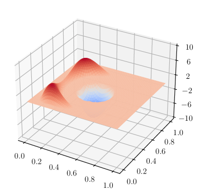
(a)

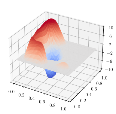
(b)

Figure 1: For $\alpha=10^{-3}$ and discretization parameter $n=64$, nominal critical point, that is, a critical point of (39) (left), and a reference critical point of (1), that is, a critical point of (37) (right).

We consider an instance of (1). Let $d=2$ and $D=(0,1)^{d}$. For $\gamma\geq 0$, let $\psi(u)=\gamma\|u\|_{L^{1}(D)}$ if $u\in L^{2}(D)$ with $-10\leq u\leq 10$ and $\psi(u)=\infty$ otherwise. We define $\Xi=[-1,1]^{100}$, $q(t)=t^{3}$, and $\langle A(\xi)y,v\rangle_{H^{-1}(D),H_{0}^{1}(D)}=\int_{D}\kappa(x,\xi)\nabla y(x)^{T}\nabla v(x)\mathrm{d}x$, where $\kappa:\bar{D}\times\Xi\to\real$ is given by $\kappa(x,\xi)=\mathrm{e}^{\sum_{k=1}^{25}5/(2k^{2})\sin(4k\xi_{k}\pi x_{1})\sin(4k\pi\xi_{25+k}x_{2})}$ if $x_{1}\leq 1/2$ and $\kappa(x,\xi)=3/2+\sum_{k=1}^{25}|(10/k^{2})\xi_{25+k}\cos((10+\xi_{25+k})x_{1}x_{2})|$ otherwise. We further define $y_{d}(x)=-1$ if $x\in[1/4,3/4]^{2}$ and $y_{d}(x)=1$ otherwise, $b(x,\xi)=1+\sum_{k=1}^{25}(5/k^{2})\xi_{75+k}x_{1}x_{2}\cos(4\pi kx_{1})\sin(4\pi kx_{2})$ if $x_{1}\leq 3/4+\xi_{76}/2$ and $b(x,\xi)=1+|\sum_{k=1}^{25}(3/k^{2})x_{2}\xi_{75+k}\sin(3\pi x_{2})\cos(3\pi(x_{1}-k\xi_{75+k}x_{2}))|$ otherwise, and $g(x,\xi)=\max\{1,\sum_{k=1}^{25}(10/k^{2})\xi_{50+k}\sin((4+k)\xi_{50+k}x_{1}x_{2})\cos((4+k)\xi_{50+k}x_{1}x_{2})\}$. The random variables $\xi_{1},\ldots,\xi_{100}$ are independent $[-1,1]$-uniformly distributed. The random fields $\kappa$, $b$, and $g$ are nonsmooth. Their definitions have been guided by the desire to design an instance of (2) with random fields that lack a representation as a linear combination of a moderate number of $L^{2}(D)$-orthogonal basis functions and of functions that are separable with respect to the vector $x$ and the parameters $\xi_{1},\ldots,\xi_{100}$. In particular, each of the random fields $\kappa$, $b$, and $g$ lacks a respresentation as a truncated Karhunen–Loève-type expansion with a small number of addends.

We discretized (1) and (3) using a finite element discretization; $H_{0}^{1}(D)$ is approximated using piecewise linear continuous finite elements and $L^{2}(D)$ is discretized using piecewise constant functions defined on a regular triangular mesh with a total of $2n^{2}$ triangles. Here, $n$ is the number of triangles in each direction in $(0,1)^{2}$. For a fixed $n\in\mathbb{N}$, the finite dimensional control space is denote by $U_{n}$. We use the subscript $n$ in $J_{n}$ and $\nabla\hat{F}_{N,n}$ to denote the approximations of $J$ (see (9)) and $\nabla\hat{F}_{N}$, respectively, resulting from the finite dimensional approximations.

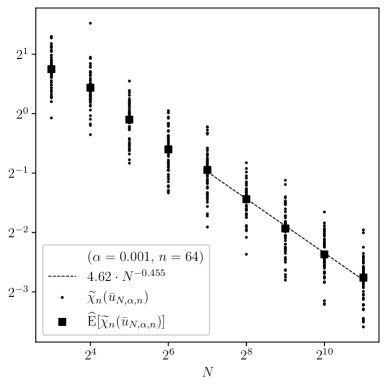
(a)

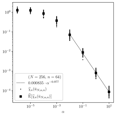
(b)

Figure 2: For $n=64$, empirical estimate $\widehat{\mathrm{E}}[\widetilde{\chi}_{n}(\bar{u}_{N,\alpha,n})]$ of $\mathbb{E}[\widetilde{\chi}_{n}(\bar{u}_{N,\alpha,n})]$ over $N$ with $\alpha=10^{-3}$ (left) and empirical estimate $\widehat{\mathrm{E}}[\widetilde{\chi}_{n}(\bar{u}_{N,\alpha,n})]$ of $\mathbb{E}[\widetilde{\chi}_{n}(\bar{u}_{N,\alpha,n})]$ over $\alpha$ with $N=256$ (right). Here, $\bar{u}_{N,\alpha,n}$ are SAA critical points of (38) computed with sample size $N$, regularization parameter $\alpha$, and discretization parameter $n$. The approximated criticality measure $\widetilde{\chi}_{n}$ is defined in (36). For both plots, $48$ independent realizations of the criticality measure $\widetilde{\chi}_{n}(\bar{u}_{N,\alpha,n})$ are depicted. The convergence rates were computed using least squares. For each plot, the first four empirical means were excluded for the least squares computations.

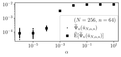
(a)

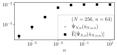
(b)

Figure 3: For $n=64$ and $N=256$, empirical mean $\widehat{\mathrm{E}}[\widetilde{\Psi}_{n}(\bar{u}_{N,\alpha,n})]$ of $\mathbb{E}[\widetilde{\Psi}_{n}(\bar{u}_{N,\alpha,n})]$ over $\alpha$ (left) and empirical mean $\widehat{\mathrm{E}}[\hat{\Psi}_{N,n}(\bar{u}_{N,\alpha,n})]$ of $\mathbb{E}[\hat{\Psi}_{N,n}(\bar{u}_{N,\alpha,n})]$ over $\alpha$ (right). Here, $\bar{u}_{N,\alpha,n}$ are the SAA critical points of (38) used in Figure 2 (right). The criticality measures $\widetilde{\Psi}_{n}$ and $\hat{\Psi}_{N,n}$ are defined in (41).

The criticality measure $\chi$ in (33) involves the gradient $\nabla F(\cdot)=\mathbb{E}[\nabla_{u}J(\cdot,\xi)]$. To approximate $\chi$, we generated $N_{1}=2^{13}$ samples using a Sobol’ sequence [36] and transformed the samples to take values in $\Xi$. Let us denote these samples by $\widetilde{\xi}_{1},\ldots,\widetilde{\xi}_{N_{1}}$. Defining $\widetilde{F}_{N_{1},n}(\cdot)=(1/N_{1})\sum_{i=1}^{N_{1}}J_{n}(\cdot,\widetilde{\xi}_{i})$, the criticality measure $\chi$ is approximated by $\widetilde{\chi}_{n}:L^{2}(D)\to[0,\infty)$ defined by

(36) $$\widetilde{\chi}_{n}(u)=\|u-\mathrm{prox}_{\psi/\alpha}({-(1/\alpha)\nabla\widetilde{F}_{N_{1},n}(u)})\|_{L^{2}(D)}.$$

We also use the samples $\widetilde{\xi}_{1},\ldots,\widetilde{\xi}_{N_{1}}$ to approximate the risk-neutral PDE-constrained optimization problem (1) by the finite dimensional SAA problem

(37) $$\min_{u\in U_{n}}\,\frac{1}{N_{1}}\sum_{i=1}^{N_{1}}J_{n}(u,\widetilde{\xi}_{i})+(\alpha/2)\|u\|_{L^{2}(D)}^{2}+\psi(u).$$

Finally, we approximate the infinite dimensional SAA problems (3) by the finite dimensional SAA problems

(38) $$\min_{u\in U_{n}}\,\frac{1}{N}\sum_{i=1}^{N}J_{n}(u,\xi^{i})+(\alpha/2)\|u\|_{L^{2}(D)}^{2}+\psi(u).$$

Inspired by the choice made in [60, p. 199], we chose $\gamma=0.2\hat{\gamma}_{\max}$, where $\hat{\gamma}_{\max}=\|\nabla\hat{F}_{10,64}(0)\|_{L^{\infty}(D)}$. We rounded $0.2\hat{\gamma}_{\max}$ to three significant figures, yielding $\gamma=7.48\cdot 10^{-3}$. This value is used for all simulations. The computations used to generate the simulation output depicted in Figures 1, 2, 4, and 5 were performed on a Linux cluster with 48 CPUs (Intel Xeon CPU E7-8857 v2 3.00GHz) and 1TB of RAM. Figure 3 is based on output of simulations performed on the PACE Phoenix cluster [59]. We used dolfin-adjoint [55, 18] with FEniCs [1, 48] to evaluate the cost functions and their derivatives. The problems (37) and (38) were solved using a semismooth Newton-CG method applied to a normal map [49, 77]. Its implementation is based on that of Moola’s NewtonCG method [57]. We present numerical illustrations for moderate values of the space discretization parameter $n$ and sample size $N$. These parameter choices are aimed at balancing the empirical demonstration of our theoretical findings with computational resource use.

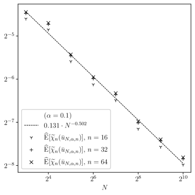
(a)

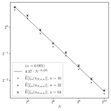
(b)

Figure 4: For multiple values of the discretization parameter $n$, empirical estimates $\widehat{\mathrm{E}}[\widetilde{\chi}_{n}(\bar{u}_{N,\alpha,n})]$ of $\mathbb{E}[\widetilde{\chi}_{n}(\bar{u}_{N,\alpha,n})]$ over $N$ with $\alpha=10^{-1}$ (left) and with $\alpha=10^{-3}$ (right). Here, $\bar{u}_{N,\alpha,n}$ are SAA critical points of (38) computed with sample size $N$, regularization parameter $\alpha$, and discretization parameter $n$. The approximated criticality measure $\widetilde{\chi}_{n}$ is defined in (36). After averaging the empirical estimates for each $N$, the convergence rates were computed using least squares.

For visualization, critical points were interpolated to the discretized state space. For $\alpha=10^{-3}$ and $n=64$, Figure 1 depicts a nominal critical point, that is, a critical point of the nominal problem

(39) $$\min_{u\in U_{n}}\,J_{n}(u,\mathbb{E}[\xi])+(\alpha/2)\|u\|_{L^{2}(D)}^{2}+\psi(u)$$

and a critical point of (37). Throughout the section, we estimate $\mathbb{E}[\widetilde{\chi}_{n}(\bar{u}_{N,\alpha,n})]$ using $48$ independent realizations of the SAA critical point $\bar{u}_{N,\alpha,n}$ of (38) and denote the empirical estimate by $\widehat{\mathrm{E}}[\widetilde{\chi}_{n}(\bar{u}_{N,\alpha,n})]$.

For $n=64$, Figure 2 depicts the empirical estimate of $\mathbb{E}[\widetilde{\chi}_{n}(\bar{u}_{N,\alpha,n})]$ with $\alpha=10^{-3}$ and shows the typical Monte Carlo convergence rate $1/\sqrt{N}$. Figure 2 also depicts the empirical estimate of $\mathbb{E}[\widetilde{\chi}_{n}(\bar{u}_{N,\alpha,n})]$ for various values of $\alpha$, which highlights a dependence on the expected error of SAA critical points on the parameter $\alpha$. To shed some light on the convergence behavior of the empirical estimate of $\mathbb{E}[\widetilde{\chi}_{n}(\bar{u}_{256,\alpha,64})]$ for $\alpha\to 0^{+}$ as depicted in Figure 2, we interpret (1), (37), and (38) as PDE-constrained optimization problems resulting from a Tikhonov regularization [15, pp. 29–37] with regularization parameter $\alpha$ and empirically demonstrate that $\bar{u}_{256,\alpha,64}$ provide approximate critical points of the optimization problems

(40) $$\min_{u\in U_{n}}\,\frac{1}{N_{1}}\sum_{i=1}^{N_{1}}J_{n}(u,\widetilde{\xi}_{i})+\psi(u)\quad\text{and}\quad\min_{u\in U_{n}}\,\frac{1}{N}\sum_{i=1}^{N}J_{n}(u,\xi^{i})+\psi(u)$$

as $\alpha\to 0^{+}$. We define $\widetilde{\Psi}_{n}$, $\hat{\Psi}_{N,n}\colon L^{2}(D)\to[0,\infty)$ by

(41) $$\begin{aligned} \widetilde{\Psi}_{n}(u)&=\|u-\mathrm{prox}_{\psi}({u-\nabla\widetilde{F}_{N_{1},n}(u)})\|_{L^{2}(D)},\\ \hat{\Psi}_{N,n}(u)&=\|u-\mathrm{prox}_{\psi}({u-\nabla\hat{F}_{N,n}(u)})\|_{L^{2}(D)}.\end{aligned}$$

The function $\widetilde{\Psi}_{n}$ is a criticality measure for the first problem in (40) and $\hat{\Psi}_{N,n}$ is one for the second problem in (40); cf., e.g., [54, sect. 2.1.2]. Figure 3 depicts the empirical mean of $\widetilde{\Psi}_{64}(\bar{u}_{256,\alpha,64})$ and $\hat{\Psi}_{256,64}(\bar{u}_{256,\alpha,64})$ computed using $48$ independent SAA critical points $\bar{u}_{256,\alpha,64}$ for various values of $\alpha$. This may suggest that the controls $\bar{u}_{256,\alpha,64}$ provide approximate critical points of the optimization problems in (40) as $\alpha\to 0^{+}$.

Figure 4 depicts the empirical estimates of $\mathbb{E}[\widetilde{\chi}_{n}(\bar{u}_{N,\alpha,n})]$ over the sample size $N$ for multiple values of the discretization parameter $n$. For fixed sample sizes $N$ and regularization parameters $\alpha$, Figure 5 depicts empirical estimates of $\mathbb{E}[\widetilde{\chi}_{n}(\bar{u}_{N,\alpha,n})]$ for multiple discretization parameters $n$. The simulation output in Figures 4 and 5 indicates that the expectation $\mathbb{E}[\widetilde{\chi}_{n}(\bar{u}_{N,\alpha,n})]$ may be independent of the discretization parameter $n$ and hence of the dimension $2n^{2}$ of the finite dimensional control space $U_{n}$. The theoretical analysis of this empirical observation is beyond the scope of this manuscript and is left as a topic for future research. For risk-neutral linear PDE-constrained optimization, the SAA approach with finite dimensional approximations of the control and state spaces are analyzed in [33, 50, 52] with respect to proximity of finite dimensional SAA solutions to the “true” optimal control.

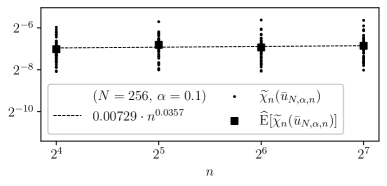
(a)

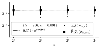
(b)

Figure 5: Empirical estimate $\widehat{\mathrm{E}}[\widetilde{\chi}_{n}(\bar{u}_{N,\alpha,n})]$ of $\mathbb{E}[\widetilde{\chi}_{n}(\bar{u}_{N,\alpha,n})]$ over the discretization parameter $n$ with $N=256$ and $\alpha=10^{-1}$ (left) and with $N=256$ and $\alpha=10^{-3}$ (right). Here, $\bar{u}_{N,\alpha,n}$ are SAA critical points of (38) computed with sample size $N$, regularization parameter $\alpha$, and discretization parameter $n$. The approximated criticality measure $\widetilde{\chi}_{n}$ is defined in (36). For both plots, $48$ independent realizations of the criticality measure $\widetilde{\chi}_{n}(\bar{u}_{N,\alpha,n})$ are depicted. The convergence rates were computed using least squares.

8 Discussion

We established nonasymptotic sample size estimates for SAA critical points of risk-neutral semilinear PDE-constrained optimization, a class of infinite dimensional, nonconvex stochastic programs. To derive the sample size estimates, we constructed a compact subset of the feasible set containing all SAA critical points. Using covering numbers of Sobolev function classes, we derived nonasymptotic sample size estimates inspired by the analyses in [67, 70, 69]. The construction of the compact set exploits structure in PDE-constrained optimization problems. This structure has been used for other purposes in different ways, such as for establishing mesh-independence of semismooth Newton methods [31], developing smoothing steps within semismooth Newton methods [77], and deriving higher regularity of solutions to deterministic PDE-constrained optimization problems [11].

Risk-neutral semilinear PDE-constrained optimization is a subfield of infinite dimensional optimization with dynamical systems under uncertainty. Our approach to establishing sample size estimates may be applied to risk-neutral PDE-constrained optimization problems other than those considered here. Among other things, our derivations rely on the Lipschitz continuity properties of the reduced parameterized objective function’s gradient and covering numbers of a set containing all SAA critical points. These key properties may be verified for objective functions other than tracking-type functions (9) and parameterized operator equations other than the semilinear PDE (2).

Risk-averse PDE-constrained optimization [21, 41, 42] provides a more general approach to optimization of complex systems under uncertainty than risk-neutral optimization. For risk-averse semilinear PDE-constrained optimization using the average/conditional value-at-risk, our analysis when combined with considerations in [47, sect. 4.2] may be adapted to constructing a compact set containing all SAA critical points. While deriving sample size estimates for critical points is complicated by the risk-averse objective function’s nonsmoothness, establishing sample size estimates for optimal values and optimal solutions may be possible using uniform exponential tail bounds.

Using Theorem 5.1, the dependence on the dimension $d$ in the sample size estimates (27) and (29) could be improved to $d/2$ if there exists $R_{\text{ad}}>0$ such that $\nabla_{u}J(u,\xi)\in H^{2}(D)$ and $\|\nabla_{u}J(u,\xi)\|_{H^{2}(D)}\leq R_{\text{ad}}$ for all $(u,\xi)\in U_{\text{ad}}\times\Xi$. However, the constant $R_{\text{ad}}^{\mathscr{D}}$ in (27) and in (29) must then be replaced by $R_{\text{ad}}$ which could be significantly larger than $R_{\text{ad}}^{\mathscr{D}}$. For a class of linear elliptic PDEs with random inputs, $H^{2}(D)$-stability estimates are provided in [72]. These stability estimates could be used to establish $\|\nabla_{u}J(u,\xi)\|_{H^{2}(D)}\leq R_{\text{ad}}$ for all $(u,\xi)\in U_{\text{ad}}\times\Xi$, provided that the parameterized elliptic operator $A$ satisfies additional assumptions.

Appendix A Measurability of set inclusions

We establish a measurability statement of set inclusions which is used in Section 6. This statement is essentially known. As introduced in Section 2, $(\Theta,\mathcal{A},\mu)$ is a complete probability space.

Lemma A.1.

Let $X$ be a real, separable Banach space and let $\Gamma:\Theta\rightrightarrows X$ be a measurable set-valued mapping with closed, nonempty images. If $\Upsilon\subset X$ is nonempty and closed, then $\{\,\theta\in\Theta\colon\,\Gamma(\theta)\subset\Upsilon\,\}$ is measurable.

Proof A.2.

Since $X\setminus\Upsilon$ is open and $\Gamma$ is measurable, $\Gamma^{-1}(X\setminus\Upsilon)$ is measurable. Combined with $\{\,\theta\in\Theta\colon\,\Gamma(\theta)\subset\Upsilon\,\}=\Theta\setminus\Gamma^{-1}(X\setminus\Upsilon)$, we find that $\{\,\theta\in\Theta\colon\,\Gamma(\theta)\subset\Upsilon\,\}$ is measurable.

Appendix B Sub-Gaussian-type bounds for maxima of random vectors

We establish expectation and exponential tail bounds for pointwise maxima of sub-Gaussian-type Hilbert space-valued random vectors. The techniques used to derive these results are similar to those used to establish expectation and tail bounds for pointwise maxima of sub-Gaussian real-valued random variables. However, we use [62, Thm. 3] which provides expectation bounds for sums of independent, mean-zero Hilbert space-valued random vectors. The results established in this section are used in Appendix C to derive uniform expectation and exponential tail bounds.

Proposition B.1.

Let $\tau>0$, let $H$ be a real, separable Hilbert space and for each $k\in\{1,2,\ldots,K\}$, let $W_{i,k}:\Theta\to H$ ($i=1,2,\ldots,N$) be independent, mean-zero random vectors with $\mathbb{E}[\cosh(\lambda\|W_{i,k}\|_{H})]\leq\exp(\lambda^{2}\tau^{2}/2)$ for all $\lambda\in\real$ and $i\in\{1,2,\ldots,N\}$. We define $Z_{k}^{[N]}=(1/N)\sum_{i=1}^{N}W_{i,k}$. Then for each $\varepsilon\geq 0$,

(42) $$\mathbb{E}[\max_{1\leq k\leq K}\|Z_{k}^{[N]}\|_{H}] \leq\sqrt{3/2}\tau(1/\sqrt{N})\sqrt{2\ln(2K)},$$

(43) $$\mathrm{Prob}(\max_{1\leq k\leq K}\|Z_{k}^{[N]}\|_{H}\geq\varepsilon) \leq 2K\exp(-\tau^{-2}\varepsilon^{2}N/3).$$

The proof of Proposition B.1 is presented at the end of the section. Let $Z:\Theta\to\real$ be a random variable. We provide a motivation for the condition

(44) $$\mathbb{E}[\cosh(\lambda|Z|)]\leq\exp(\lambda^{2}\tau^{2}/2)\quad\text{for all}\quad\lambda\in\real,$$

where $\tau>0$. A random variable $Z:\Theta\to\real$ is sub-Gaussian with parameter $\tau$ if $\tau\in[0,\infty)$ and $\mathbb{E}[\exp(\lambda Z)]\leq\exp(\lambda^{2}\tau^{2}/2)$ for all $\lambda\in\real$ [10, p. 9]. Since $\cosh(x)=(\mathrm{e}^{-x}+\mathrm{e}^{x})/2$ for all $x\in\real$, a sub-Gaussian random variable $Z$ with parameter $\tau>0$ fulfills (44). If $H$ is a real, separable Hilbert space and $W:\Theta\to H$ is a nondegenerate, mean-zero Gaussian random vector, then (44) holds with $Z=\|W\|_{H}$ and $\tau=\mathbb{E}[\|W\|_{H}^{2}]^{1/2}$ [62, Rem. 4]. Suppose that there exists $\sigma>0$ such that

(45) $$\mathbb{E}[\exp(|Z|^{2}/\sigma^{2})]\leq\mathrm{e}.$$

This condition and its variants are used in the literature on stochastic programming [56, 69, 46] with $Z$ being the norm of a stochastic (sub)gradient, for example. Let us demonstrate that (44) and (45) are essentially equivalent.

Lemma B.2.

Let $Z:\Theta\to\real$ be a random variable.

1. If (44) holds with $\tau>0$, then (45) holds with $\sigma=(2\tau^{2}/(1-\mathrm{e}^{-2}))^{1/2}$.

2. If (45) is satisfied with $\sigma>0$, then (44) is fulfilled with $\tau=2^{1/4}\sigma$.

3. If $\tau>0$ and $|Z|\leq\tau$ w.p. $1$, then (44) is fulfilled.

Proof B.3.

1. We adapt the proof of [10, Lem. 1.6 on p. 9]. We define $s=1-\mathrm{e}^{-2}$ and $\sigma^{2}=2\tau^{2}/s$. We have for all $z\in\real$ (cf.  [10, p. 9]),

   $$\int\mathrm{e}^{\lambda^{2}\tau^{2}(s-1)/(2s)}\mathrm{d}\lambda=\tfrac{1}{\tau}\sqrt{\tfrac{2\pi s}{1-s}}\quad\text{and}\quad\int\cosh(\lambda z)\mathrm{e}^{-\lambda^{2}\tau^{2}/(2s)}\mathrm{d}\lambda=\tfrac{\sqrt{2\pi s}}{\tau}\mathrm{e}^{z^{2}/\sigma^{2}}.$$

   Multiplying (44) by $\mathrm{e}^{-\lambda^{2}\tau^{2}/(2s)}$ yields $\mathbb{E}[\cosh(\lambda|Z|)\mathrm{e}^{-\lambda^{2}\tau^{2}/(2s)}]\leq\mathrm{e}^{\lambda^{2}\tau^{2}(s-1)/(2s)}$ for all $\lambda\in\real$. Integrating both sides over $\lambda\in\real$ and using Fubini’s theorem, we obtain $\tfrac{\sqrt{2\pi s}}{\tau}\mathbb{E}[\mathrm{e}^{|Z|^{2}/\sigma^{2}}]\leq\tfrac{1}{\tau}\sqrt{\tfrac{2\pi s}{1-s}}$. Hence, $\mathbb{E}[\mathrm{e}^{|Z|^{2}/\sigma^{2}}]\leq 1/(1-s)^{1/2}=\mathrm{e}$.

2. The proof is inspired by that of [69, Prop. 9.81]. Fix $\lambda\in\real$ with $\lambda^{2}\sigma^{2}/2\leq 1$. Using Jensen’s inequality and $\cosh(x)\leq\exp(x^{2}/2)$ for all $x\in\real$ [76, eq. (4.6.6)],

   $$\mathbb{E}[\cosh(\lambda|Z|)]\leq\mathbb{E}[\mathrm{e}^{\lambda^{2}|Z|^{2}/2}]=\mathbb{E}[\mathrm{e}^{\lambda^{2}\sigma^{2}|Z|^{2}/(2\sigma^{2})}]\leq\mathbb{E}[\mathrm{e}^{|Z|^{2}/\sigma^{2}}]^{\lambda^{2}\sigma^{2}/2}\leq\mathrm{e}^{\lambda^{2}\sigma^{2}/2}.$$

   Now let $\lambda\in\real$ with $\lambda^{2}\sigma^{2}/2>1$. Young’s inequality ensures $2\lambda s\leq\lambda^{2}\sigma^{2}/\sqrt{2}+\sqrt{2}s^{2}/\sigma^{2}$ for all $s\in\real$. Combined with $\cosh(x)\leq\exp(x)$ being valid for all $x\geq 0$, the symmetry of $\cosh$, $\sqrt{2}\lambda^{2}\sigma^{2}/4>\sqrt{2}/2$, and Jensen’s inequality, we have

   $$\mathbb{E}[\cosh(\lambda|Z|)]\leq\mathrm{e}^{\lambda^{2}\sigma^{2}/(2\sqrt{2})}\mathbb{E}[\mathrm{e}^{\sqrt{2}|Z|^{2}/(2\sigma^{2})}]\leq\mathrm{e}^{\lambda^{2}\sigma^{2}/(2\sqrt{2})+\sqrt{2}/2}<\mathrm{e}^{\sqrt{2}\lambda^{2}\sigma^{2}/2}.$$

   Putting together the pieces, we obtain the assertion.

3. Since $\cosh(x)\leq\exp(x^{2}/2)$ for all $x\in\real$ [76, eq. (4.6.6)] and $\cosh$ is a symmetric function, we have $\mathbb{E}[\cosh(\lambda|Z|)]\leq\cosh(\lambda\tau)\leq\exp(\lambda^{2}\tau^{2}/2)$ for all $\lambda\in\real$.

Lemma B.4.

Let $\tau>0$, let $H$ be a real, separable Hilbert space, and let $Z_{i}:\Theta\to H$ be independent, mean-zero random vectors such that $\mathbb{E}[\cosh(\lambda\|Z_{i}\|_{H})]\leq\exp(\lambda^{2}\tau^{2}/2)$ for all $\lambda\in\real$ ($i=1,2,\ldots,N$). Then, for each $\lambda\in\real$,

$$\mathbb{E}[\cosh(\lambda\|Z_{1}+\cdots+Z_{N}\|_{H})]\leq\exp(3\lambda^{2}\tau^{2}N/4).$$

Lemma B.4 is established using Theorem B.5.

Theorem B.5 (see [62, Thm. 3]).

Let $H$ be a real, separable Hilbert space. If $Z_{i}:\Theta\to H$ $(i=1,\ldots,N)$ are independent, mean-zero random vectors, then

$$\mathbb{E}[\cosh(\lambda\|Z_{1}+\cdots+Z_{N}\|_{H})]\leq\prod_{i=1}^{N}\mathbb{E}[\exp(\lambda\|Z_{i}\|_{H})-\lambda\|Z_{i}\|_{H}]\quad\text{for all}\quad\lambda\geq 0.$$

Proof B.6 (Proof of Lemma B.4).

Fix $\lambda\geq 0$. We have $\exp(s)-s\leq\cosh(\sqrt{3/2}s)$ for all $s\in\real$. Hence, $\mathbb{E}[\exp(\lambda\|Z_{i}\|_{H})-\lambda\|Z_{i}\|_{H}]\leq\exp(3\lambda^{2}\tau^{2}/4)$. Combined with Theorem B.5, we find that $\mathbb{E}[\cosh(\lambda\|Z_{1}+\cdots+Z_{N}\|_{H})]\leq\prod_{i=1}^{N}\exp(3\lambda^{2}\tau^{2}/4)=\exp(3\lambda^{2}\tau^{2}N/4)$. Since $\cosh$ is symmetric, the estimate is valid for all $\lambda\in\real$.

Lemma B.7 establishes an expectation and an exponential tail bound for pointwise maxima of sub-Gaussian random variables similar to those found, e.g., in [17, Prop. 7.29] and [9, sect. 2.5], but we express sub-Gaussianity via (44).

Lemma B.7.

Let $\sigma>0$. Suppose that $Z_{k}:\Theta\to\real$ are random variables with $\mathbb{E}[\cosh(\lambda|Z_{k}|)]\leq\exp(\lambda^{2}\sigma^{2}/2)$ for all $\lambda\in\real$ and $k=1,2,\ldots,K$. Then for all $\varepsilon>0$,

$$\mathbb{E}[\max_{1\leq k\leq K}|Z_{k}|]\leq\sigma\sqrt{2\ln(2K)}\quad\text{and}\quad\mathrm{Prob}(\max_{1\leq k\leq K}|Z_{k}|\geq\varepsilon)\leq 2K\mathrm{e}^{-\varepsilon^{2}/(2\sigma^{2})}.$$

Proof B.8.

The proof of the expectation bound uses standard derivations based on “smoothing” of the pointwise maximum. We have $\exp\leq 2\cosh$. For $\lambda>0$, we have

$$\mathbb{E}[\max_{1\leq k\leq K}|Z_{k}|] \leq(1/\lambda)\ln\Big{(}\sum_{k=1}^{K}\mathbb{E}[\exp(\lambda|Z_{k}|)]\Big{)}\leq(1/\lambda)\ln\Big{(}\sum_{k=1}^{K}2\mathbb{E}[\cosh(\lambda|Z_{k}|)]\Big{)}$$

$$\leq(1/\lambda)\ln\big{(}2K\exp(\lambda^{2}\sigma^{2}/2)\big{)}=(1/\lambda)\ln(2K)+\lambda^{2}\sigma^{2}/2.$$

Choosing $\lambda=\sqrt{2\ln(2K)}/\sigma$ yields the expectation bound.

The union bound and Markov’s inequality ensure for all $\lambda>0$,

$$\mathrm{Prob}(\max_{1\leq k\leq K}|Z_{k}|\geq\varepsilon) \leq\sum_{k=1}^{K}\mathrm{Prob}(|Z_{k}|\geq\varepsilon)\leq\mathrm{e}^{-\lambda\varepsilon}\sum_{k=1}^{K}\mathbb{E}[\exp(\lambda|Z_{k}|)]$$

$$\!\!\leq 2\mathrm{e}^{-\lambda\varepsilon}\sum_{k=1}^{K}\mathbb{E}[\cosh(\lambda|Z_{k}|)]\leq 2K\mathrm{e}^{-\lambda\varepsilon}\mathrm{e}^{\lambda^{2}\sigma^{2}/2}=2K\mathrm{e}^{-\lambda\varepsilon+\lambda^{2}\sigma^{2}/2}.$$

Minimizing the right-hand side over $\lambda>0$ yields the tail bound.

Proof B.9 (Proof of Proposition B.1).

We prove (42) and (43) using Lemmas B.4 and B.7. Fix $\lambda\geq 0$. Lemma B.4 and $\mathbb{E}[\cosh(\lambda\|W_{i,k}\|_{H})]\leq\exp(\lambda^{2}\tau^{2}/2)$ imply

$$\mathbb{E}[\cosh(\lambda\|Z_{k}^{[N]}\|_{H})]\leq\exp(3\lambda^{2}\tau^{2}/(4N)).$$

Defining $\sigma=\tau\sqrt{3/2}/\sqrt{N}$, we have $\exp(3\lambda^{2}\tau^{2}/(4N))=\exp(\lambda^{2}\sigma^{2}/2)$. Now we apply Lemma B.7 to the random variables $\|Z_{k}^{[N]}\|_{H}$, yielding (42) and (43).

Appendix C Uniform exponential tail bounds for SAA normal maps

We derive uniform expectation and exponential tail bounds for an SAA normal map in Hilbert spaces. The derivation of the tail bounds is inspired by those in [69, Thms. 9.84 and 9.86] for real-valued functions. The uniform exponential tail bounds are used in Section 6 to derive nonasymptotic sample size estimates.

Throughout the section, $\xi$, $\Xi$, $\xi^{1},\xi^{2},\ldots$ and $(\Omega,\mathcal{F},P)$ are as in Sections 1 and 3. Let $H$ be a real, separable Hilbert space and let $\varphi:H\to(-\infty,\infty]$ be proper, convex and lower semicontinuous. We define $H_{\text{ad}}=\{\,u\in H\colon\,\varphi(u)<\infty\,\}$. Let $G:H_{\text{ad}}\times\Xi\to H$ be a function. We define $\hat{G}_{N}:H_{\text{ad}}\to H$ by $\hat{G}_{N}(u)=(1/N)\sum_{i=1}^{N}G(u,\xi^{i})$. Let $\alpha>0$. We further define $\Phi$, $\hat{\Phi}_{N}:H\to H$ by

$$\Phi(v)=\mathbb{E}[G(\mathrm{prox}_{\varphi/\alpha}({v}),\xi)]\quad\text{and}\quad\hat{\Phi}_{N}(v)=\hat{G}_{N}(\mathrm{prox}_{\varphi/\alpha}({v})).$$

Since $\xi^{1},\xi^{2},\ldots$ are defined on $\Omega$, we can view $\hat{\Phi}_{N}$ as a function on $H\times\Omega$. The mappings $v\mapsto\Phi(v)+\alpha v$ and $v\mapsto\hat{\Phi}_{N}(v)+\alpha v$ define normal maps [63]. When establishing the uniform tail bounds in Proposition C.3, we only rely on properties of their difference, that is, on characteristics of $\Phi-\hat{\Phi}_{N}$. The following assumptions are inspired by those used in [69, sect. 9.2.11]. A random variable $Z:\Theta\to\real$ is sub-exponential with parameters $(\tau,\Lambda)$ if $\tau\in[0,\infty)$, $\Lambda\in(0,\infty]$ and $\mathbb{E}[\exp(\lambda Z)]\leq\exp(\lambda^{2}\tau^{2}/2)$ for all $\lambda\in(-\Lambda,\Lambda)$ [10, p. 19].

[Uniform exponential tail bounds: Problem data]

1. The mapping $G:H_{\text{ad}}\times\Xi\to H$ is a Carathéodory function, and $G(u,\xi)$ is Bochner integrable for each $u\in H_{\text{ad}}$.

2. For an integrable random variable $M:\Xi\to(0,\infty)$,

   $$\|G(u_{2},\xi)-G(u_{1},\xi)\|_{H}\leq M(\xi)\|u_{2}-u_{1}\|_{H}\quad\text{for all}\quad u_{2},u_{1}\in H_{\text{ad}},\;\;\xi\in\Xi.$$

3. The random variable $M(\xi)-\mathbb{E}[M(\xi)]$ is sub-exponential with parameters $(\tau_{M},\Lambda_{M})$.

4. There exists $\tau_{G}>0$ such that, for each $u\in H_{\text{ad}}$,

   (46) $$\mathbb{E}[\cosh(\lambda\|G(u,\xi)-\mathbb{E}[G(u,\xi)]\|_{H})]\leq\exp(\lambda^{2}\tau_{G}^{2}/2)\quad\text{for all}\quad\lambda\in\real.$$

5. The $\nu$-covering number of the nonempty, closed set $V_{\text{ad}}\subset H_{\text{ad}}$ is finite for all $\nu>0$.

 (e) ensures that $V_{\text{ad}}$ is compact, as it is closed and totally bounded [44, Lem. 8.2-2]. We define $\hat{M}_{N}=(1/N)\sum_{i=1}^{N}M(\xi^{i})$.

Lemma C.1.

If  (a) and  (b) hold, then $\Phi$ and $\hat{\Phi}_{N}$ are Lipschitz continuous with Lipschitz constants $\mathbb{E}[M(\xi)]$ and $\hat{M}_{N}$, respectively. Moreover $\sup_{v\in V_{\text{ad}}}\,\|\hat{\Phi}_{N}(v)-\Phi(v)\|_{H}$ is measurable on $\Omega$.

Proof C.2.

For each $u\in H_{\text{ad}}$, $\mathbb{E}[G(u,\xi)]$ is well-defined. Hence,  (b) ensures that $\mathbb{E}[G(\cdot,\xi)]$ is Lipschitz continuous on $H_{\text{ad}}$ with Lipschitz constant $\mathbb{E}[M(\xi)]$. Since $\mathrm{prox}_{\varphi/\alpha}$ is firmly nonexpansive and $\mathrm{prox}_{\varphi/\alpha}({H})\subset H_{\text{ad}}$, $\Phi$ is Lipschitz continuous with Lipschitz constant $\mathbb{E}[M(\xi)]$. Similarly, we obtain that $\hat{\Phi}_{N}$ is Lipschitz continuous with Lipschitz constant $\hat{M}_{N}$. Combined with the fact that $G$ is a Carathéodory mapping on $H_{\text{ad}}\times\Xi$ and that $\xi^{i}:\Omega\to\Xi$ ($i=1,2,\ldots$) are random elements, we find that $\|\hat{\Phi}_{N}(\cdot)-\Phi(\cdot)\|_{H}$ is a Carathéodory map on $H_{\text{ad}}\times\Omega$. Since $V_{\text{ad}}\subset H_{\text{ad}}$ is nonempty and closed, $\sup_{v\in V_{\text{ad}}}\,\|\hat{\Phi}_{N}(v)-\Phi(v)\|_{H}$ is measurable [29, Lem. 2.1].

Proposition C.3.

Let Appendix C hold. Then $\Phi$ is Lipschitz continuous with Lipschitz constant $L=\mathbb{E}[M(\xi)]$ and for all $\nu>0$,

(47) $$\mathbb{E}[\sup_{v\in V_{\text{ad}}}\,\|\hat{\Phi}_{N}(v)-\Phi(v)\|_{H}]\leq 2L\nu+\tfrac{\sqrt{3}\tau_{G}}{\sqrt{N}}\sqrt{\ln(2\mathcal{N}(\nu;V_{\text{ad}},\|\cdot\|_{H}))}.$$

Define $\ell=L^{2}/(2\tau_{M}^{2})$ if $L\leq\Lambda_{M}\tau_{M}^{2}$ and $\ell=\Lambda_{M}L/2$ otherwise. Then for all $\varepsilon>0$,

$$\mathrm{Prob}(\sup_{v\in V_{\text{ad}}}\,\|\hat{\Phi}_{N}(v)-\Phi(v)\|_{H}\geq\varepsilon)\leq\mathrm{e}^{-N\ell}+2\mathcal{N}(\varepsilon/(4L);V_{\text{ad}},\|\cdot\|_{H})\mathrm{e}^{-N\varepsilon^{2}/(48\tau_{G}^{2})}.$$

If furthermore $M(\xi)\leq L$ for all $\xi\in\Xi$, then for all $\varepsilon>0$,

(48) $$\mathrm{Prob}(\sup_{v\in V_{\text{ad}}}\,\|\hat{\Phi}_{N}(v)-\Phi(v)\|_{H}\geq\varepsilon)\leq 2\mathcal{N}(\varepsilon/(4L);V_{\text{ad}},\|\cdot\|_{H})\mathrm{e}^{-N\varepsilon^{2}/(48\tau_{G}^{2})}.$$

Before establishing Proposition C.3, we illustrate how it is used in Section 6 to derive nonasymptotic sample size estimates.

Remark C.4.

Let the hypotheses of Proposition C.3 hold. Suppose that w.p. $1$ for each $N\in\mathbb{N}$, $\{\,v\in H\colon\,\hat{\Phi}_{N}(v)+\alpha v=0\,\}$ is contained in $V_{\text{ad}}$. Let $N\in\mathbb{N}$ and let $v_{N}\in H$ be a measurable selection of $\{\,v\in H\colon\,\hat{\Phi}_{N}(v)+\alpha v=0\,\}$. Then w.p. $1$,

$$\|\alpha v_{N}+\Phi(v_{N})\|_{H} \leq\|\hat{\Phi}_{N}(v_{N})-\Phi(v_{N})\|_{H}+\|\hat{\Phi}_{N}(v_{N})+\alpha v_{N}\|_{H}$$

$$\leq\sup_{v\in V_{\text{ad}}}\,\|\hat{\Phi}_{N}(v)-\Phi(v)\|_{H}.$$

The term on the right-hand side can be estimated using Proposition C.3.

We establish Proposition C.3 using Lemma C.5, which is a direct consequence of [10, Thm. 5.1 on p. 26].

Lemma C.5.

Let $W$ be an integrable, nonnegative random variable. Suppose that $W-\mathbb{E}[W]$ is sub-exponential with parameters $(\tau,\Lambda)$. We define $L=\mathbb{E}[W]$. Let $\ell=L^{2}/(2\tau^{2})$ if $L\leq\Lambda\tau^{2}$ and $\ell=\Lambda L/2$ otherwise. If $W_{1},W_{2},\ldots$ are independent and each $W_{i}:\Theta\to\real$ has the same distribution as $W$, then for all $N\in\mathbb{N}$, $\mathrm{Prob}((1/N)\sum_{i=1}^{N}W_{i}\geq 2L)\leq\exp(-N\ell)$.

Proof C.6.

Since $W_{i}-\mathbb{E}[W]$ are independent and sub-exponential with parameters $(\tau,\Lambda)$, we have (see [10, Thm. 5.1 on p. 26]),

$$\mathrm{Prob}\Big{(}\frac{1}{N}\sum_{i=1}^{N}W_{i}-\mathbb{E}[W]\geq\varepsilon\Big{)}\leq\begin{cases}\exp(-N\varepsilon^{2}/(2\tau^{2}))&\text{if}\quad 0<\varepsilon\leq\Lambda\tau^{2},\\ \exp(-N\Lambda\varepsilon/2)&\text{if}\quad\varepsilon>\Lambda\tau^{2}.\end{cases}$$

Choosing $\varepsilon=\mathbb{E}[W]$ and using the definition of $\ell$, we obtain the assertion.

Proof C.7 (Proof of Proposition C.3).

The proof is inspired by those of [69, Thms. 9.84 and 9.86]. The Lipschitz property of $\Phi$ is provided by Lemma C.1. Fix $\nu>0$. We define $K=\mathcal{N}(\nu;V_{\text{ad}},\|\cdot\|_{H})<\infty$. By assumption, there exist $v_{1},\ldots,v_{K}\in H$ such that for each $v\in V_{\text{ad}}$, we have $\|v-v_{k(v)}\|_{H}\leq\nu$, where $k(v)=\operatorname*{arg\,min}_{1\leq k\leq K}\,\|v-v_{k}\|_{H}$. Furthermore, $G(u,\xi)-\mathbb{E}[G(u,\xi)]$ has zero mean for each $u\in H_{\text{ad}}$. Using Lemma C.1, we find that

$$\begin{aligned} \|\hat{\Phi}_{N}(v)-\Phi(v)\|_{H}&\leq\|\hat{\Phi}_{N}(v)-\hat{\Phi}_{N}(v_{k(v)})\|_{H}+\|\hat{\Phi}_{N}(v_{k(v)})-\Phi(v_{k(v)})\|_{H}\\ &\quad+\|\Phi(v_{k(v)})-\Phi(v)\|_{H}\\ &\leq\hat{M}_{N}\|v-v_{k(v)}\|_{H}+\|\hat{\Phi}_{N}(v_{k(v)})-\Phi(v_{k(v)})\|_{H}+L\|v-v_{k(v)}\|_{H}\\ &\leq\hat{M}_{N}\nu+\|\hat{\Phi}_{N}(v_{k(v)})-\Phi(v_{k(v)})\|_{H}+L\nu.\end{aligned}$$

Defining $u_{k}=\mathrm{prox}_{\varphi/\alpha}({v_{k}})$, we obtain $u_{k}\in H_{\text{ad}}$ and

$$\begin{aligned} \sup_{v\in V_{\text{ad}}}\,\|\hat{\Phi}_{N}(v)-\Phi(v)\|_{H}&\leq\hat{M}_{N}\nu+\max_{1\leq k\leq K}\,\|\hat{G}_{N}(u_{k})-\mathbb{E}[G(u_{k},\xi)]\|_{H}+L\nu.\end{aligned}$$

Taking expectations, using $\mathbb{E}[\hat{M}_{N}]=L$ and utilizing Proposition B.1, we obtain (47).

We fix $\varepsilon>0$ and choose $\nu=\varepsilon/(4L)$ as in [69, p. 471]. Proposition B.1 ensures

$$\mathrm{Prob}(\max_{1\leq k\leq K}\,\|\hat{G}_{N}(u_{k})-\mathbb{E}[G(u_{k},\xi)]\|_{H}\geq\varepsilon/4)\leq 2K\mathrm{e}^{-N\varepsilon^{2}/(48\tau_{G}^{2})}.$$

Lemma C.5 yields $\mathrm{Prob}(\hat{M}_{N}\geq 2L)\leq\exp(-N\ell)$. If $\hat{M}_{N}<2L$, then $(\hat{M}_{N}+L)\nu<3L\nu$. Now the union bound implies the first tail bound. If $M(\xi)\leq L$, then $\mathrm{Prob}(\hat{M}_{N}\geq 2L)=0$ and we obtain (48).

References

- [1] M. S. Alnæs, J. Blechta, J. Hake, A. Johansson, B. Kehlet, A. Logg, C. Richardson, J. Ring, M. E. Rognes, and G. N. Wells, The FEniCS Project Version 1.5, Arch. Numer. Software, 3 (2015), pp. 9–23, https://doi.org/10.11588/ans.2015.100.20553.
- [2] J.-P. Aubin and H. Frankowska, Set-Valued Analysis, Mod. Birkhäuser Class., Springer, Boston, 2009, https://doi.org/10.1007/978-0-8176-4848-0.
- [3] H. H. Bauschke and P. L. Combettes, Convex Analysis and Monotone Operator Theory in Hilbert Spaces, CMS Books Math., Springer, New York, 2011, https://doi.org/10.1007/978-1-4419-9467-7.
- [4] P. Benner, S. Dolgov, A. Onwunta, and M. Stoll, Low-rank solution of an optimal control problem constrained by random Navier-Stokes equations, Internat. J. Numer. Methods Fluids, 92 (2020), pp. 1653–1678, https://doi.org/10.1002/fld.4843.
- [5] M. Š. Birman and M. Z. Solomjak, Piecewise-polynomial approximations of functions of the classes , Math. USSR Sb., 2 (1967), pp. 295–317, https://doi.org/10.1070/sm1967v002n03abeh002343.
- [6] M. Š. Birman and M. Z. Solomjak, Quantitative Analysis in Sobolev Imbedding Theorems and Applications to Spectral Theory, Amer. Math. Soc. Transl. Ser. 2, 114, AMS, Providence, RI, 1980, https://doi.org/10.1090/trans2/114. Translated from the Russian by F. A. Cezus.
- [7] J. F. Bonnans and A. Shapiro, Perturbation Analysis of Optimization Problems, Springer Ser. Oper. Res., Springer, New York, 2000, https://doi.org/10.1007/978-1-4612-1394-9.
- [8] A. Borzì and V. Schulz, Computational Optimization of Systems Governed by Partial Differential Equations, Comput. Sci. Eng. 8, SIAM, Philadelphia, PA, 2011, https://doi.org/10.1137/1.9781611972054.
- [9] S. Boucheron, G. Lugosi, and P. Massart, Concentration Inequalities: A Nonasymptotic Theory of Independence, Oxford University Press, Oxford, 2013, https://doi.org/10.1093/acprof:oso/9780199535255.001.0001.
- [10] V. V. Buldygin and Yu. V. Kozachenko, Metric Characterization of Random Variables and Random Processes, Transl. Math. Monogr. 188, AMS, Providence, RI, 2000, https://doi.org/10.1090/mmono/188. Translated by V. Zaiats.
- [11] E. Casas, R. Herzog, and G. Wachsmuth, Optimality conditions and error analysis of semilinear elliptic control problems with cost functional, SIAM J. Optim., 22 (2012), pp. 795–820, https://doi.org/10.1137/110834366.
- [12] M. Chen, S. Mehrotra, and D. Papp, Scenario generation for stochastic optimization problems via the sparse grid method, Comput. Optim. Appl., 62 (2015), pp. 669–692, https://doi.org/10.1007/s10589-015-9751-7.
- [13] J. B. Conway, A Course in Functional Analysis, Grad. Texts in Math. 96, Springer, New York, 1985, https://doi.org/10.1007/978-1-4757-3828-5.
- [14] F. Cucker and S. Smale, On the mathematical foundations of learning, Bull. Amer. Math. Soc. (N.S.), 39 (2002), pp. 1–49, https://doi.org/10.1090/S0273-0979-01-00923-5.
- [15] A. L. Dontchev and T. Zolezzi, Well-posed optimization problems, Lecture Notes in Math. 1543, Springer, Berlin, 1993, https://doi.org/10.1007/BFb0084195.
- [16] D. E. Edmunds and H. Triebel, Function Spaces, Entropy Numbers, Differential Operators, Cambridge Tracts in Math., Cambridge University Press, 1996, https://doi.org/10.1017/CBO9780511662201.
- [17] S. Foucart and H. Rauhut, A Mathematical Introduction to Compressive Sensing, Appl. Numer. Harmon. Anal., Birkhäuser, Bosten, 2013, https://doi.org/10.1007/978-0-8176-4948-7.
- [18] S. W. Funke and P. E. Farrell, A framework for automated PDE-constrained optimisation, preprint, https://arxiv.org/abs/1302.3894, 2013.
- [19] S. W. Funke, S. C. Kramer, and M. D. Piggott, Design optimisation and resource assessment for tidal-stream renewable energy farms using a new continuous turbine approach, Renew. Energ., 99 (2016), pp. 1046–1061, https://doi.org/10.1016/j.renene.2016.07.039.
- [20] S. Garreis, Optimal Control under Uncertainty: Theory and Numerical Solution with Low-Rank Tensors, Dissertation, Technische Universität München, München, 2019, https://nbn-resolving.de/urn/resolver.pl?urn:nbn:de:bvb:91-diss-20190215-1452538-1-1.
- [21] S. Garreis, T. M. Surowiec, and M. Ulbrich, An interior-point approach for solving risk-averse PDE-constrained optimization problems with coherent risk measures, SIAM J. Optim., 31 (2021), pp. 1–19, https://doi.org/10.1137/19M125039X.
- [22] S. Garreis and M. Ulbrich, Constrained optimization with low-rank tensors and applications to parametric problems with PDEs, SIAM J. Sci. Comput., 39 (2017), pp. A25–A54, https://doi.org/10.1137/16M1057607.
- [23] S. Garreis and M. Ulbrich, A fully adaptive method for the optimal control of semilinear elliptic PDEs under uncertainty using low-rank tensors, tech. report, Technische Universität München, München, 2019.
- [24] S. Garreis and M. Ulbrich, An inexact trust-region algorithm for constrained problems in Hilbert space and its application to the adaptive solution of optimal control problems with PDEs, tech. report, Technische Universität München, München, 2019.
- [25] C. Geiersbach and T. Scarinci, Stochastic proximal gradient methods for nonconvex problems in Hilbert spaces, Comput. Optim. Appl., 78 (2021), pp. 705–740, https://doi.org/10.1007/s10589-020-00259-y.
- [26] P. Grisvard, Elliptic Problems in Nonsmooth Domains, Classics Appl. Math. 69, SIAM, Philadelphia, PA, 2011, https://doi.org/10.1137/1.9781611972030.
- [27] V. Guigues, A. Juditsky, and A. Nemirovski, Non-asymptotic confidence bounds for the optimal value of a stochastic program, Optim. Methods Softw., 32 (2017), pp. 1033–1058, https://doi.org/10.1080/10556788.2017.1350177.
- [28] P. A. Guth, V. Kaarnioja, F. Y. Kuo, C. Schillings, and I. H. Sloan, A quasi-Monte Carlo method for optimal control under uncertainty, SIAM/ASA J. Uncertain. Quantif., 9 (2021), pp. 354–383, https://doi.org/10.1137/19M1294952.
- [29] F. Hiai and H. Umegaki, Integrals, conditional expectations, and martingales of multivalued functions, J. Multivariate Anal., 7 (1977), pp. 149–182, https://doi.org/10.1016/0047-259X(77)90037-9.
- [30] E. Hille and R. S. Phillips, Functional Analysis and Semi-Groups, Colloq. Publ. 31, AMS, Providence, RI, 1957, https://doi.org/10.1090/coll/031.
- [31] M. Hintermüller and M. Ulbrich, A mesh-independence result for semismooth Newton methods, Math. Program., 101 (2004), pp. 151–184, https://doi.org/10.1007/s10107-004-0540-9.
- [32] M. Hinze, R. Pinnau, M. Ulbrich, and S. Ulbrich, Optimization with PDE Constraints, Math. Model. Theory Appl. 23, Springer, Dordrecht, 2009, https://doi.org/10.1007/978-1-4020-8839-1.
- [33] M. Hoffhues, W. Römisch, and T. M. Surowiec, On quantitative stability in infinite-dimensional optimization under uncertainty, Optim. Lett., 15 (2021), pp. 2733–2756, https://doi.org/10.1007/s11590-021-01707-2.
- [34] P. J. Huber, The behavior of maximum likelihood estimates under nonstandard conditions, in Proceedings of the Fifth Berkeley Symposium on Mathematical Statistics and Probability, Volume 1: Statistics, L. M. Le Cam and J. Neyman, eds., Berkeley, CA, 1967, University of California Press, pp. 221–233.
- [35] T. Hytönen, J. van Neerven, M. Veraar, and L. Weis, Analysis in Banach Spaces: Martingales and Littlewood-Paley Theory, Ergeb. Math. Grenzgeb. (3) 63, Springer, Cham, 2016, https://doi.org/10.1007/978-3-319-48520-1.
- [36] S. Joe and F. Y. Kuo, Constructing Sobol’ sequences with better two-dimensional projections, SIAM J. Sci. Comput., 30 (2008), pp. 2635–2654, https://doi.org/10.1137/070709359.
- [37] V. Kaňková, An approximative solution of a stochastic optimization problem, in Transactions of the Eighth Prague Conference: on Information Theory, Statistical Decision Functions, Random Processes held at Prague, from August 28 to September 1, 1978 Volume A, Czechoslovak Acad. Sci. 8A, Springer, Dordrecht, 1978, pp. 349–353, https://doi.org/10.1007/978-94-009-9857-5_33.
- [38] A. J. Kleywegt, A. Shapiro, and T. Homem-de Mello, The sample average approximation method for stochastic discrete optimization, SIAM J. Optim., 12 (2002), pp. 479–502, https://doi.org/10.1137/S1052623499363220.
- [39] D. P. Kouri, M. Heinkenschloss, D. Ridzal, and B. van Bloemen Waanders, A trust-region algorithm with adaptive stochastic collocation for PDE optimization under uncertainty, SIAM J. Sci. Comput., 35 (2013), pp. A1847–A1879, https://doi.org/10.1137/120892362.
- [40] D. P. Kouri, M. Heinkenschloss, D. Ridzal, and B. G. van Bloemen Waanders, Inexact objective function evaluations in a trust-region algorithm for PDE-constrained optimization under uncertainty, SIAM J. Sci. Comput., 36 (2014), pp. A3011–A3029, https://doi.org/10.1137/140955665.
- [41] D. P. Kouri and A. Shapiro, Optimization of PDEs with uncertain inputs, in Frontiers in PDE-Constrained Optimization, H. Antil, D. P. Kouri, M.-D. Lacasse, and D. Ridzal, eds., IMA Vol. Math. Appl. 163, Springer, New York, NY, 2018, pp. 41–81, https://doi.org/10.1007/978-1-4939-8636-1_2.
- [42] D. P. Kouri and T. M. Surowiec, Risk-averse PDE-constrained optimization using the conditional value-at-risk, SIAM J. Optim., 26 (2016), pp. 365–396, https://doi.org/10.1137/140954556.
- [43] D. P. Kouri and T. M. Surowiec, Risk-averse optimal control of semilinear elliptic PDEs, ESAIM Control. Optim. Calc. Var., 26 (2020), https://doi.org/10.1051/cocv/2019061.
- [44] E. Kreyszig, Introductory Functional Analysis with Applications, John Wiley & Sons, New York, NY, 1978.
- [45] K. Kunisch and D. Walter, Semiglobal optimal feedback stabilization of autonomous systems via deep neural network approximation, ESAIM Control Optim. Calc. Var., 27 (2021), https://doi.org/10.1051/cocv/2021009.
- [46] G. Lan, First-order and Stochastic Optimization Methods for Machine Learning, Springer Ser. Data Sci., Springer, Cham, 2020, https://doi.org/10.1007/978-3-030-39568-1.
- [47] G. Lan, A. Nemirovski, and A. Shapiro, Validation analysis of mirror descent stochastic approximation method, Math. Program., 134 (2012), pp. 425–458, https://doi.org/10.1007/s10107-011-0442-6.
- [48] A. Logg, K.-A. Mardal, and G. N. Wells, eds., Automated Solution of Differential Equations by the Finite Element Method: The FEniCS Book, Lect. Notes Comput. Sci. Eng. 84, Springer, Berlin, 2012, https://doi.org/10.1007/978-3-642-23099-8.
- [49] F. Mannel and A. Rund, A hybrid semismooth quasi-Newton method for nonsmooth optimal control with PDEs, Optim. Eng., 22 (2021), pp. 2087–2125, https://doi.org/10.1007/s11081-020-09523-w.
- [50] M. Martin, S. Krumscheid, and F. Nobile, Complexity analysis of stochastic gradient methods for PDE-constrained optimal control problems with uncertain parameters, ESAIM Math. Model. Numer. Anal., 55 (2021), pp. 1599–1633, https://doi.org/10.1051/m2an/2021025.
- [51] S. Mei, Y. Bai, and A. Montanari, The landscape of empirical risk for nonconvex losses, Ann. Statist., 46 (2018), pp. 2747–2774, https://doi.org/10.1214/17-AOS1637.
- [52] J. Milz, Reliable error estimates for optimal control of linear elliptic PDEs with random inputs, arXiv preprint arXiv:2206.09160, (2022), https://arxiv.org/abs/2206.09160.
- [53] J. Milz, Sample average approximations of strongly convex stochastic programs in Hilbert spaces, Optim. Lett., 17 (2023), pp. 471–492, https://doi.org/10.1007/s11590-022-01888-4.
- [54] A. Milzarek, X. Xiao, S. Cen, Z. Wen, and M. Ulbrich, A stochastic semismooth Newton method for nonsmooth nonconvex optimization, SIAM J. Optim., 29 (2019), pp. 2916–2948, https://doi.org/10.1137/18M1181249.
- [55] S. K. Mitusch, S. W. Funke, and J. S. Dokken, dolfin-adjoint 2018.1: automated adjoints for FEniCS and Firedrake, J. Open Source Softw., 4 (2019), p. 1292, https://doi.org/10.21105/joss.01292.
- [56] A. Nemirovski, A. Juditsky, G. Lan, and A. Shapiro, Robust stochastic approximation approach to stochastic programming, SIAM J. Optim., 19 (2009), pp. 1574–1609, https://doi.org/10.1137/070704277.
- [57] M. Nordaas and S. W. Funke, The Moola optimisation package, https://github.com/funsim/moola, 2016.
- [58] E. Novak, Deterministic and Stochastic Error Bounds in Numerical Analysis, Lecture Notes in Math. 1349, Springer, Berlin, 1988, https://doi.org/10.1007/BFb0079792.
- [59] PACE, Partnership for an Advanced Computing Environment (PACE), 2017, http://www.pace.gatech.edu.
- [60] N. Parikh and S. Boyd, Proximal Algorithms, Found. Trends Mach. Learning, 1 (2014), pp. 127–239, https://doi.org/10.1561/2400000003, https://web.stanford.edu/~boyd/papers/pdf/prox_algs.pdf.
- [61] C. Phelps, J. Royset, and Q. Gong, Optimal control of uncertain systems using sample average approximations, SIAM J. Control Optim., 54 (2016), pp. 1–29, https://doi.org/10.1137/140983161.
- [62] I. F. Pinelis and A. I. Sakhanenko, Remarks on inequalities for large deviation probabilities, Theory Probab. Appl., 30 (1986), pp. 143–148, https://doi.org/10.1137/1130013.
- [63] S. M. Robinson, Normal maps induced by linear transformations, Math. Oper. Res., 17 (1992), pp. 691–714, https://doi.org/10.1287/moor.17.3.691.
- [64] W. Römisch and T. M. Surowiec, Asymptotic properties of Monte Carlo methods in elliptic PDE-constrained optimization under uncertainty, arXiv preprint arXiv:2106.06347, (2021), https://arxiv.org/abs/2106.06347.
- [65] J. O. Royset, Approximations of semicontinuous functions with applications to stochastic optimization and statistical estimation, Math. Program., 184 (2020), pp. 289–318, https://doi.org/10.1007/s10107-019-01413-z.
- [66] S. Shalev-Shwartz, O. Shamir, N. Srebro, and K. Sridharan, Learnability, stability and uniform convergence, J. Mach. Learn. Res., 11 (2010), pp. 2635–2670, https://jmlr.csail.mit.edu/papers/volume11/shalev-shwartz10a/shalev-shwartz10a.pdf.
- [67] A. Shapiro, Monte Carlo Sampling Methods, in Stochastic Programming, Handbooks in Oper. Res. Manag. Sci. 10, Elsevier, 2003, pp. 353–425, https://doi.org/10.1016/S0927-0507(03)10006-0.
- [68] A. Shapiro, Stochastic programming approach to optimization under uncertainty, Math. Program., 112 (2008), pp. 183–220, https://doi.org/10.1007/s10107-006-0090-4.
- [69] A. Shapiro, D. Dentcheva, and A. Ruszczyński, Lectures on Stochastic Programming: Modeling and Theory, MOS-SIAM Ser. Optim., SIAM, Philadelphia, PA, 3rd ed., 2021, https://doi.org/10.1137/1.9781611976595.
- [70] A. Shapiro and A. Nemirovski, On complexity of stochastic programming problems, in Continuous Optimization: Current Trends and Modern Applications, V. Jeyakumar and A. Rubinov, eds., Appl. Optim. 99, Springer, Boston, MA, 2005, pp. 111–146, https://doi.org/10.1007/0-387-26771-9_4.
- [71] G. Stadler, Elliptic optimal control problems with -control cost and applications for the placement of control devices, Comput. Optim. Appl., 44 (2009), pp. 159–181, https://doi.org/10.1007/s10589-007-9150-9.
- [72] A. L. Teckentrup, R. Scheichl, M. B. Giles, and E. Ullmann, Further analysis of multilevel Monte Carlo methods for elliptic PDEs with random coefficients, Numer. Math., 125 (2013), pp. 569–600, https://doi.org/10.1007/s00211-013-0546-4.
- [73] H. Tiesler, R. M. Kirby, D. Xiu, and T. Preusser, Stochastic collocation for optimal control problems with stochastic PDE constraints, SIAM J. Control Optim., 50 (2012), pp. 2659–2682, https://doi.org/10.1137/110835438.
- [74] V. M. Tikhomirov, -entropy and -capacity of sets in functional spaces, in Selected Works of A. N. Kolmogorov: Volume III: Information Theory and the Theory of Algorithms, A. N. Shiryayev, ed., Math. Appl. 27, Springer, Dordrecht, 1993, pp. 86–170, https://doi.org/10.1007/978-94-017-2973-4_7.
- [75] F. Tröltzsch, Optimal Control of Partial Differential Equations: Theory, Methods and Applications, Grad. Stud. Math. 112, AMS, Providence, RI, 2010, https://doi.org/10.1090/gsm/112. Translated by J. Sprekels.
- [76] J. A. Tropp, An introduction to matrix concentration inequalities, Found. Trends Mach. Learn., 8 (2015), pp. 1–230, https://doi.org/10.1561/2200000048.
- [77] M. Ulbrich, Semismooth Newton Methods for Variational Inequalities and Constrained Optimization Problems in Function Spaces, MOS-SIAM Ser. Optim., SIAM, Philadelphia, PA, 2011, https://doi.org/10.1137/1.9781611970692.
- [78] F. Wechsung, A. Giuliani, M. Landreman, A. J. Cerfon, and G. Stadler, Single-stage gradient-based stellarator coil design: stochastic optimization, Nuclear Fusion, 62 (2022), p. 076034, https://doi.org/10.1088/1741-4326/ac45f3.
- [79] M. J. Zahr, K. T. Carlberg, and D. P. Kouri, An efficient, globally convergent method for optimization under uncertainty using adaptive model reduction and sparse grids, SIAM/ASA J. Uncertain. Quantif., 7 (2019), pp. 877–912, https://doi.org/10.1137/18M1220996.
- [80] E. Zeidler, Nonlinear Functional Analysis and its Applications II/B: Nonlinear Monotone Operators, Springer, New York, 1990, https://doi.org/10.1007/978-1-4612-0981-2.