Graph Neural Networks for Channel Decoding

Abstract

In this work, we propose a fully differentiable graph neural network (GNN)-based architecture for channel decoding and showcase a competitive decoding performance for various coding schemes, such as low-density parity-check (LDPC) and BCH codes. The idea is to let a neural network (NN) learn a generalized message passing algorithm over a given graph that represents the forward error correction (FEC) code structure by replacing node and edge message updates with trainable functions. Contrary to many other deep learning-based decoding approaches, the proposed solution enjoys scalability to arbitrary block lengths and the training is not limited by the curse of dimensionality. We benchmark our proposed decoder against state-of-the-art in conventional channel decoding as well as against recent deep learning-based results. For the (63,45) BCH code, our solution outperforms weighted belief propagation (BP) decoding by approximately 0.4 dB with significantly less decoding iterations and even for 5G NR LDPC codes, we observe a competitive performance when compared to conventional BP decoding. For the BCH codes, the resulting GNN decoder can be fully parametrized with only 9640 weights.

I Introduction

Codes on graphs [1, 2, 3] have become the workhorse of modern forward error correction (FEC) schemes and have, thereby, brought the theoretical asymptotic performance limits of channel coding within practical reach [4, 5, 6]. As a result, many practical coding schemes in today’s wireless communication systems can be interpreted as (sparse) graphs which inherently provide a low-complexity, iterative message passing decoder—namely, belief propagation (BP) decoding [7, 8]. However, when focusing on short to intermediate codeword lengths, the decoding performance under BP decoding shows a non-negligible gap when compared to maximum likelihood (ML) decoding for most codes [9]. For this regime, there is still no universal iterative coding scheme as either the decoding graph becomes dense (e.g., for Polar decoding [10]) and/or the decoding graph has many short cycles. For instance, finding an iterative decoding scheme for short length CRC-aided Polar codes is an active field of research [11]. Further, finding universal decoding algorithms for Polar, low-density parity-check (LDPC), and BCH codes in the same hardware engine may simplify the chip design of future wireless systems.

In the recent years, the field of deep learning for communications has rapidly progressed and showcased several impressive results ranging from fully neural network (NN)-based orthogonal frequency division multiplexing (OFDM) receivers [12] via weighted BP decoding [13] up to end-to-end optimization of the complete transceiver signal processing chain [14]. However, even though the idea of incorporating expert domain knowledge in the NN structure has been investigated many times [13, 15], there is still no structured way of embedding a known graph (or data) structure in current deep learning architectures. Deep learning for communications is therefore often doomed by the curse of dimensionality [16, 17], meaning that the training complexity is exponential in the number of information bits. As a result, most current learning approaches in the literature [18, 19] besides weighted BP decoding [13] are limited by their scalability and tend to have a tremendous amount of trainable parameters (in the range of millions of weights even for short codes). These schemes require expensive re-training–or to store and load pre-calculated parameters–for every set of new code parameters.

From a more philosophical point-of-view, we have not yet found the NN architectures that suit well to channel coding tasks, similar to what convolutional neural networks (CNNs) are for computer vision and transformers are for natural language processing, respectively. Thus, we believe that the obvious close relations between factor graphs [3] and graph neural networks (GNNs) [20], render them into a promising architecture for trainable decoders. We refer the interested reader to [21] for a more general view on GNNs.

The idea of using message passing neural networks (MPNNs) [22] for channel decoding has been recently introduced in [20] and the authors of [23] use GNNs to support the design of Polar codes. Inspired by these results, we aim to provide an introduction to GNNs for channel decoding tasks and to understand their advantages and limitations. Please note that the authors in [20] augment BP decoding by the combination with a GNN while in our work, we propose a fully learned decoder. Our main contribution is to

• Present a fully differentiable GNN-based decoder for linear binary block codes;

• Clarify terminology and translate the GNN terminology to the channel coding domain;

• Benchmark against state-of-the-art 5G NR LDPC and BCH codes;

• Provide design guidelines for GNN decoders and interpretation of an extensive hyperparameter optimization;

• Support reproducible research: the source code is implemented with Sionna [24] and is available online.

It is worth a note that many of today’s problems in communications can be formulated by the framework of factor graphs [3, 25]. We would like to emphasize our fascination for this omnipresence of graphs in many communications problems and the fact that we still do not have a universal framework to embed such graphs in our NN designs. We intend this paper to be a first step towards such a framework. However, we do not want to oversell the results in this well-investigated field of channel coding which has already seen many powerful hand-crafted solutions. We rather hope this paper opens more research questions than it answers.

$$\mathbf{H}=\begin{bmatrix}\color[rgb]{1,0,0}1&\color[rgb]{1,0,0}1&\color[rgb]{1,0,0}1&0&\color[rgb]{1,0,0}1&0&0\\ \color[rgb]{0.55078125,0.77734375,0.2421875}1&\color[rgb]{0.55078125,0.77734375,0.2421875}1&0&\color[rgb]{0.55078125,0.77734375,0.2421875}1&0&\color[rgb]{0.55078125,0.77734375,0.2421875}1&0\\ \color[rgb]{0,0.4921875,0.77734375}1&0&\color[rgb]{0,0.4921875,0.77734375}1&\color[rgb]{0,0.4921875,0.77734375}1&0&0&\color[rgb]{0,0.4921875,0.77734375}1\color[rgb]{0,0,0}\end{bmatrix}$$

(a) Parity-check matrix.

(b) Tanner graph.

Figure 1: Bipartite graph for the (7,4) Hamming code.

II GNNs for Channel Decoding

We consider a binary linear block code $\mathcal{C}$ of length $n$ that can be described by a binary parity-check matrix $\mathbf{H}^{(n-k)\times n}\in\mathbb{F}_{2}^{(n-k)\times n}$ where each codeword represents $k$ information bits. A binary vector is a codeword $\mathbf{c}\in\mathbb{F}_{2}^{n}$ of $\mathcal{C}$ iff in GF(2) it holds that $\mathbf{H}\mathbf{c}^{\text{T}}=\mathbf{0}$. For the additive white Gaussian noise (AWGN) channel with noise variance $\sigma_{\text{ch}}^{2}$ and binary phase shift keying (BPSK) modulation $\mathbf{x}=-2\mathbf{c}+1$, the receiver observes $\mathbf{y}=\mathbf{x}+\mathbf{n}$ with $\mathbf{n}\sim\mathcal{N}(\mathbf{0},\sigma_{\text{ch}}^{2}\mathbf{I})$. After demapping, the log-likelihood ratio (LLR) of the $i$th codeword bit $c_{i}$ is given as

$$\ell_{\text{ch},i}=\operatorname{log}\frac{p(c_{i}=0)}{p(c_{i}=1)}=\frac{2y_{i}}{\sigma_{\text{ch}}^{2}}$$

and $\boldsymbol{\ell}_{\text{ch}}$ denotes the vector of all $n$ channel LLRs.

The optimal bitwise ML decoder performs

$$\hat{c_{i}}=\operatorname{argmax}_{c_{i}\in\{0,1\}}p(\mathbf{y}|c_{i})\quad\forall i=0,\dots,n-1.$$

It is worth mentioning, that some decoders provide ML-sequence estimation (i.e., minimize the BLER) such as the Viterbi decoder while others are ML bitwise estimators (i.e., minimize the BER) such as the BCJR decoder. As a result of bitwise ML decoding, $\hat{\mathbf{c}}$ is not necessarily a valid codeword.

By interpreting $\mathbf{H}$ as bipartite graph [26], we immediately get a decoding graph for message passing decoding. As illustrated in Fig. 1, each row of $\mathbf{H}$ represents a single parity-check (so-called constraint or check node (CN)) and each column represents a codeword position (so-called variable node (VN)). For finite length, BP is known to be suboptimal due to cycles in the decoding graph (no tree structure). For a detailed introduction to BP decoding, we refer to [27, 2] and would like to emphasize a few important properties:

• $\mathbf{H}$ is not unique and can be modified (e.g., by the linear combination of rows), i.e., multiple graphs can be assigned to the same code (see [1]). Thus, several graph properties such as specific cycles or node degrees are strictly speaking not code properties.

• $\mathbf{H}$ can be also overcomplete, i.e., more than $n-k$ rows can be part of $\mathbf{H}$ which are then linearly dependent (see [28] for a practical application in decoding).

• The set of all $2^{k}$ codewords $\mathbf{c}$ defines the code $\mathcal{C}$. However, for a linear code, the code is fully defined by $k$ linearly independent codewords (see curse of dimensionality in [17]).

• For a linear code, the all-zero codeword $\mathbf{c}=\mathbf{0}$ is always part of the code as $\mathbf{H}\mathbf{0}^{\text{T}}=\mathbf{0}$.

II-A Bipartite Graph Neural Network Framework

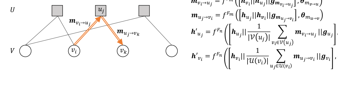
Figure 2: Graph neural network based message passing for bipartite graphs (see Alg. 1).

We now describe the bipartite GNN-based message passing decoding algorithm for a given parity-check matrix $\mathbf{H}$ following [22]. Learning the graph structure itself is also an active field of research, but not considered in this work.

Let $f^{F}(\mathbf{x},\boldsymbol{\theta}_{\text{NN}})$ denote a parametrized function that maps $f^{F}:\mathbf{x}\mapsto\mathbb{R}^{F}$ and can be parametrized by the weights $\boldsymbol{\theta}_{\text{NN}}$ (e.g., we use simple multilayer perceptrons (MLPs) throughout this work and other options are possible). Note that the superscript $F\in\mathbb{N}$ defines the dimensionality of the messages. As illustrated in Fig. 2, we operate on a bipartite graph and we introduce the following nodes/functions

• Variable node (VN): Each node $v_{i}$ represents a transmitted codeword bit $c_{i}$. Let $\mathcal{V}$ denote the set of all VNs.

• Factor node (FN): Each node $u_{j}$ represents one of the $n-k$ code constraints (i.e., check nodes in BP decoding). Let $\mathcal{U}$ denote the set of all FNs.

• The VN $v_{i}$ is connected to the FN $u_{j}$ (and vice versa) iff $H_{j,i}=1$.

• $\mathcal{V}(u_{j})$ denotes the neighborhood of $u_{j}$, i.e., the set of all variable nodes connected to factor node $u_{j}$.

• $\mathcal{U}(v_{i})$ denotes the neighborhood of $v_{i}$, i.e., the set of all factor nodes connected to variable node $v_{i}$.

• $\mathcal{E}$ denotes the set of all edges $e_{i,j}=(v_{i},u_{j})$ in the graph, i.e., $e_{i,j}=(v_{i},u_{j})\in\mathcal{E}\Leftrightarrow H_{j,i}=1$.

• Node values: Each node computes an $F_{\text{n}}$-dimensional vector $\mathbf{h}_{v_{i},}\mathbf{h}_{u_{j}}\in\mathbb{R}^{F_{\text{n}}}$ for each VN $v_{i}$ and FN $u_{j}$, respectively.

• (Directed) edge values: Each directed edge message has an assigned $F_{\text{m}}$-dimensional value $\mathbf{m}_{v_{i}\to u_{j}},\mathbf{m}_{u_{i}\to v_{j}}\in\mathbb{R}^{F_{\text{m}}}$. Remark: the values are (generally) different for each direction.

• Node attributes: Every node can have an assigned node attribute $\mathbf{g}_{v_{i}},\mathbf{g}_{u_{j}}\in\mathbb{R}^{F_{\text{na}}}$ for VN and FN, respectively. This is node specific, i.e., in total $|\mathcal{V}|+|\mathcal{U}|=2n-k$ node attributes exist.

• Edge attributes: Every edge can have an assigned edge attribute $\mathbf{g}_{m_{v_{i}\to u_{j}}},\mathbf{g}_{m_{u_{j}\to v_{i}}}\in\mathbb{R}^{F_{\text{ma}}}$, respectively. This is edge specific and depends on the edge direction, i.e., in total $2|\mathcal{E}|$ edge attributes exist. Remark: this is similar to the trainable weights in [13].

We implement the GNN decoding algorithm for bipartite graphs as MPNN [22, 20]. Therefore, we introduce two kind of trainable functions: (a) the edge message update functions and (b) the node update functions. An updated message value from VN $v_{i}$ to FN $u_{j}$ can be calculated as

$$\mathbf{m}_{v_{i}\to u_{j}}=f^{F_{\text{m}}}([\mathbf{h}_{v_{i}}||\mathbf{h}_{u_{j}}||\mathbf{g}_{m_{v_{i}\to u_{j}}}],\boldsymbol{\theta}_{m_{v\to u}})$$ (1)

where $\boldsymbol{\theta}_{m_{v\to u}}$ denotes the trainable parameters of the node update and $[\mathbf{x}||\mathbf{y}]$ denotes the concatenation of the vectors $\mathbf{x}$ and $\mathbf{y}$. Please note that the same weights $\boldsymbol{\theta}_{m_{v\to u}}$ are applied to all edges. Similarly, the updated message value from FN $u_{j}$ to VN $v_{i}$ is given as

$$\mathbf{m}_{u_{j}\to v_{i}}=f^{F_{\text{n}}}([\mathbf{h}_{u_{j}}||\mathbf{h}_{v_{i}}||\mathbf{g}_{m_{u_{j}\to v_{i}}}],\boldsymbol{\theta}_{m_{u\to v}})$$ (2)

with $\boldsymbol{\theta}_{m_{u\to v}}$ denoting another (shared) set of trainable parameters. The updated node value for VN $v_{i}$ is calculated as

$$\mathbf{h}^{\prime}_{v_{i}}=f^{F_{n}}([\mathbf{h}_{v_{i}}||\bigoplus_{u_{j}\in\mathcal{U}(v_{i})}\mathbf{m}_{u_{j}\to v_{i}}||\mathbf{g}_{v_{i}}],\boldsymbol{\theta}_{v})$$ (3)

with $\boldsymbol{\theta}_{v}$ being the (shared) parameters of the VN update function and $\bigoplus$ denotes a message aggregation function. Throughout this work, we use the sum or the mean operator for $\bigoplus$. Similarly, the FN value update can be written as

$$\mathbf{h}^{\prime}_{u_{j}}=f^{F_{n}}([\mathbf{h}_{u_{j}}||\bigoplus_{v_{i}\in\mathcal{V}(u_{j})}\mathbf{m}_{v_{i}\to u_{j}}||\mathbf{g}_{u_{j}}],\boldsymbol{\theta}_{u})$$ (4)

where $\boldsymbol{\theta}_{u}$ are the trainable parameters of the FN update.

We initialize $\mathbf{h}_{u}=\mathbf{0}$ and apply a linear input embedding $\mathbf{h}_{v_{i}}=\ell_{\text{ch},i}\times\mathbf{w}$ where $\mathbf{w}\in\mathbb{R}^{F_{\text{n}}}$ is a trainable parameter that projects the scalar $\ell_{\text{ch},i}$ to an $F_{\text{n}}$-dimensional space. After decoding, the final estimate is given by $\ell_{i}=\mathbf{q}^{t}\mathbf{h}_{v_{i}}$, where $\mathbf{q}\in\mathbb{R}^{F_{\text{n}}}$ is another trainable vector. Intuitively, projecting messages to higher dimensions can simplify its processing due to the blessing of dimensionality [29].

We now perform iterative node and message updates until reaching a maximum of $N_{\text{iter}}$ iterations. We apply the flooding scheduling, i.e., (1) is applied to all messages in the same time step (the same holds for the other updates in (2), (3), (4)). Other update schedules are possible, but not further investigated. Alg. 1 summarizes the detailed decoding algorithm.

Input : LLRs of the (noisy) channel observations $\boldsymbol{\ell}_{\text{ch}}$

Set of trainable parameters:

- FN updates $\boldsymbol{\theta}_{u}$

- VN updates $\boldsymbol{\theta}_{v}$

- Variable to factor message updates $\boldsymbol{\theta}_{m_{v\to u}}$

- Factor to variable message updates $\boldsymbol{\theta}_{m_{u\to v}}$

- VN attributes $\{\mathbf{g}_{v_{i}}\}\forall v_{i}\in\mathcal{V}$

- FN attributes $\{\mathbf{g}_{u_{j}}\}\forall u_{j}\in\mathcal{U}$

- Msg. attr.$\{\mathbf{g}_{m_{v_{i}\to u_{j}}},\mathbf{g}_{m_{u_{j}\to v_{i}}}\},\forall(v_{i},u_{j})\in\mathcal{E}$

- Input embedding $\mathbf{w}$

- Output embedding $\mathbf{q}$

Output : Soft estimates $\boldsymbol{\ell}$ of the codeword bits $\mathbf{c}$

1

2% Initialize graph nodes

3 For $v_{i}\in\mathcal{V}$ 

4       $\mathbf{h}_{v_{i}}\leftarrow\ell_{\text{ch,i}}\cdot\mathbf{w}$

5      

6

7$\mathbf{h}_{u}\leftarrow\mathbf{0}$

8 % Run decoding iterations

9 For $it=0,\dots,N_{\text{iter}}-1$ do

10       % Update variable to factor node messages

11       For $(v_{i},u_{j})\in\mathcal{E}$ 

12             $\mathbf{m}_{v_{i}\to u_{j}}\leftarrow f^{F_{\text{m}}}([\mathbf{h}_{v_{i}}||\mathbf{h}_{u_{j}}||\mathbf{g}_{v_{i}\to u_{j}}],\boldsymbol{\theta}_{m_{v\to u}})$

13      

14      % Update factor nodes

15       For $u_{j}\in\mathcal{U}$ 

16             $\mathbf{h}_{u_{j}}\leftarrow f^{F_{\text{n}}}([\mathbf{h}_{u_{j}}||\frac{1}{|\mathcal{V}(u_{j})|}\sum_{v_{i}\in\mathcal{V}(u_{j})}\mathbf{m}_{v_{i}\to u_{j}}||\mathbf{g}_{u_{j}}],\boldsymbol{\theta}_{u})$

17      

18      % Update factor to variable node messages

19       For $(v_{i},u_{j})\in\mathcal{E}$ 

20             $\mathbf{m}_{u_{j}\to v_{i}}\leftarrow f^{F_{\text{m}}}([\mathbf{h}_{u_{j}}||\mathbf{h}_{v_{i}}||\mathbf{g}_{u_{j}\to v_{i}}],\boldsymbol{\theta}_{m_{u\to v}})$

21      

22      % Update variable nodes

23       For $v_{i}\in\mathcal{V}$ 

24             $\mathbf{h}_{v_{i}}\leftarrow f^{F_{\text{n}}}([\mathbf{h}_{v_{i}}||\frac{1}{|\mathcal{U}(v_{i})|}\sum_{u_{j}\in\mathcal{U}(v_{i})}\mathbf{m}_{u_{j}\to v_{i}}||\mathbf{g}_{v_{i}}],\boldsymbol{\theta}_{v})$

25      

26      

27 end

28% Project variable node values back to scalar LLRs

29 For $v_{i}\in\mathcal{V}$ 

30       $\ell_{i}\leftarrow\mathbf{q}^{t}\mathbf{h}_{v_{i}}$

31

32return $\boldsymbol{\ell}=[\ell_{0},\dots,\ell_{n-1}]$

Algorithm 1 GNN-based Decoding Algorithm

Please note that the number of trainable weights is small when compared to state-of-the-art in literature (e.g., the BCH GNN-decoder is fully defined by 9640 parameters) and the computational complexity scales linearly in $n$. However, the proposed decoder is still of high complexity as the graph inference requires the execution of the message update functions for every incoming and outgoing edge in the graph. We leave it open for future research to optimize the decoding complexity.

II-B Training methodology

We train the GNN by applying iterative loop-unrolling [13]. All NN weights use the Glorot uniform initalizer [30] while the node/edge attributes are set to $\mathbf{0}$ in our experiments. The binary cross-entropy (BCE) loss is implemented as multi-loss over all iterations (e.g., as proposed in [13])

$$\begin{split}\mathcal{L}=\frac{1}{nN_{\text{iter}}}\sum_{it=0}^{N_{\text{iter}}-1}\sum_{i=0}^{n-1}&\left[c_{i}\operatorname{log}\left(\sigma\left(\ell_{i}^{it}\right)\right)\right.\\ &\left.+(1-c_{i})\operatorname{log}\left(1-\sigma\left(\ell_{i}^{it}\right)\right)\right]\end{split}$$ (5)

where the superscript it denotes the decoder output $\boldsymbol{\ell}$ of the $it$th iteration and $\sigma(x)=\frac{1}{1+e^{-x}}$. As can be seen later in Fig. 3, this allows for inference of the trained decoder with a variable number of iterations and enables the possibility of early stopping.

We use standard stochastic gradient descent (SGD)-based training with the Adam optimizer. Please note that the batchsize can be (relatively) small, as the same weights are applied to all nodes, which effectively multiplies the batchsize by $|\mathcal{U}|$ and $|\mathcal{V}|$, respectively (and $|\mathcal{E}|$ for the message updates). The training requires the availability of an encoder, as all-zero codeword based training is not possible. Thus, we draw new random codewords for every SGD iteration.

TABLE I: Hyperparameter search for the (63,45) BCH code

Parameter	Search space	Best
activation	{ReLU, sigmoid, tanh}	tanh
$N_{\text{iter}}$	$1-20$	8
$F_{\text{n}}$	$1-32$	20
$F_{\text{m}}$	$1-32$	20
# hidden units MLP	$4-128$	40
# MLP layers	$1-4$	2
aggregation function	{mean, sum}	mean
LLR clipping	$\{10,16,20,\infty\}$	$\infty$
learning rate	-	$10^{-3}-10^{-5}$
batchsize	-	256

As the design space of the hyperparameters is virtually infinite, we have utilized a hyperparameter search [31] and, therefore, evaluated 436 different models. Tab. I summarizes the search space and best hyperparameters. For the simulated BCH code, we did not observe any gains by having edge and node attributes and, thus, set these parameters to $\mathbf{0}$. However, it is instructive to realize that the weights of the node and message update functions are shared between all nodes (and all iterations). Thus, learning edge (or node) specific properties of a specific graph (e.g., learning to remove short cycles) requires the availability of these attributes.

One can make a few interesting observations:

• Activation: in particular for small MLP sizes, tanh often performs better than the ReLU and (logistic) sigmoid activation.

• Wide vs. deep: we found multiple architectures with a similar bit error rate (BER) performance, however, some are deeper (i.e., more iterations but less weights) while others are wider (i.e., less iterations required but more weights per update). This gives an additional degree of freedom to the system designer.

• Node aggregation: the mean aggregation function tends to show a better performance than the sum aggregation and we empirically observed an improved stability when changing the number of iterations after training.

• Bias: for scenarios with punctured nodes (e.g., due to rate-matching) deactivating the bias in the MLP layers for node/edge update functions improves the stability for exact zero input LLR messages as it automatically leads to an all-zero output.

III Results

We now evaluate the decoding performance for BCH and LDPC codes. For both codes, no node/edge attributes are used.

III-A BCH codes

Fig. 3 shows the BER performance for the learned (63,45) BCH decoder. The GNN hyperparameters are provided in Tab. I. It is worth mentioning that BP decoding of BCH codes is known to be highly suboptimal due to the high density of $\mathbf{H}$. Nonetheless, it has become a common benchmark in the literature [13, 19] to decode the (63,45) BCH code, and we therefore provide results for this class of codes. The sub-optimality of BCH provides an interesting playground for our GNN experiments as–in contrast to well-designed LDPC codes–BER performance gains when compared to BP are still possible. One of the currently best learned decoders is reported in [19]. However, the number of trainable parameters is 2-3 orders of magnitude larger compared to our decoder.

Although the decoder is trained for a fixed number of decoding iterations $N_{\text{iter}}=8$, the results in Fig. 3 show that the same weights can be used for a variable number of iterations $N_{\text{iter}}=\{2,3,4,6,8,10\}$ (with a degraded performance for fewer iterations, which is the expected behavior). This allows for the implementation of early stopping at any time. Somewhat to our surprise, the GNN-based decoder with only three decoding iterations achieves a similar BER performance when compared to the conventional BP decoder with 20 iterations.

Figure 3: BER performance for decoding of the (63,45) BCH code. The GNN was trained for $N_{\text{iter}}=8$ iterations.

III-B Regular LDPC codes

To further investigate the scalability, we train the GNN to decode regular $(v=3,c=6)$ LDPC codes with VN degree $v$ and CN degree $c$. The parity-check matrix is randomly constructed and not further optimized for BP decoding. However, the same parity-check matrix is used for both decoders. The results are shown in Fig. 4. Note that the GNN is trained for a codeword length of $n=100$ and $N_{\text{iter}}=10$ iterations. For faster training convergence and to avoid another expensive hyperparameter optimization, we increase the NN dimensions to approximately 28,700 trainable weights. As can be seen, the GNN decoder slightly outperforms BP decoding even for long codes which underlines the scalability of the GNN. However, the observed gains tend to diminish with increasing $n$.

To investigate the impact of different graphs, we re-use the trained weights of the BCH decoder from Sec. III-A to decode the LDPC code. For this, we replace the underlying graph structure but keep the weights from the previous training. As can be seen, the learned GNN decoder is unfortunately not universal and requires re-training to adopt to the new code.

Figure 4: BER performance for decoding of regular (3,6) LDPC codes of the same coderate $r=0.5$. All decoders use $N_{\text{iter}}=20$ iterations. The GNN is only trained once for $n=100$.

III-C 5G NR LDPC codes

We now train the GNN for decoding of the 5G NR LDPC code [32] and change the length after training by changing the lifting factor of the code. The GNN consists of 18,900 trainable weights. The results are shown in Fig. 5. As the 5G NR LDPC code inherently requires rate-matching, we train the GNN on the underlying (non-rate-matched) parity-check matrix and apply rate-matching only for inference. The rate-matching itself is not learned. This avoids that the first $2Z$ information bits are punctured during the training (where $Z$ denotes the lifting factor of the code). Otherwise, we empirically observed instabilities during training through the rate-matching. The results in Fig. 5 show that both decoders achieve the same decoding performance for a wide range of code parameters and for the exact code parameters used for training even a small gain can be observed. Keep in mind that the 5G LDPC code is specifically optimized for BP decoding and the evaluation is done for the AWGN channel. Intuitively, there is only little room for improvement through deep learning for this optimal setting.

As shown in Fig. 5(a), the same weights can be scaled to longer codeword lengths and the same flexibility can be also observed w.r.t. the coderate in Fig. 5(b). This could enable a simplified training based on the underlying protograph of the LDPC code and only a few sets of different weights must be stored to support all possible code parameters of a given standard. However, we would like to emphasize that the training–in particular, when rate-matching is involved– requires carefully adjusted hyperparameters which seem to be highly code specific. Note that both algorithms use flooding scheduling for their node updates and the required number of iterations may change for a different scheduling.

(a) varying length; $r=0.43$

(b) varying coderate; $n=280$

Figure 5: BER performance for decoding of the 5G NR LDPC code [32] for $N_{\text{iter}}=10$ decoding iterations. The GNN is only trained once for $(k,n)=(60,140)$.

IV Discussion and open issues

As mentioned above, this work raises more questions than it answers and, thus, we would like to state a few of them for possible future research:

• Is training of a universal GNN decoder possible? One possible way to achieve such a universality is the training of the same GNN decoder weights for multiple FEC codes in parallel.

• The effect of edge/node attributes is currently unknown. We empirically observed that the decoder does not (strongly) benefit from these attributes, but the decoding and memory complexity increases. However, when compensating for specific weaknesses of the decoding graph, these attributes may be beneficial.

• The decoding complexity of the proposed GNN is higher when compared to BP as the MLPs must be executed many times. Could different architectures for the update functions reduce the complexity?

• This work could be extended towards heterogenous GNNs such that for irregular node degrees different trainable functions are applied.

• Apply graph modifications and pruning. We empirically observe that the decoding graph is still crucial for the decoding performance. Similar to [28], pruning of the decoding graph could be applied during training.

• Extensions to non-binary codes and non-AWGN channels are possible, and we expect higher gains compared to BP decoding when operating on real-world datasets including different kinds of impairments.

V Conclusion

We have presented a GNN-based algorithm for decoding of binary linear block codes where the code structure can be directly embedded into the decoding algorithm. As a result, we achieved a competitive bit-error-rate performance for BCH codes with significantly fewer decoding iterations when compared to classical BP decoding. For LDPC codes, the performance remains competitive with BP decoding for the AWGN channel, however, adapting the decoder to different channels or even to real-world datasets is straightforward. In order not to over-sell our results, we would like to emphasize that the computational complexity of the proposed decoder is high. However, for scenarios where no suitable classical decoder is available (such as for quantum error control coding [33]), it opens an interesting avenue for future research. It remains also open how to reduce the overall decoding complexity and, thus, to improve the energy-efficiency. It seems promising to combine the presented decoder with optimized NN libraries for adaptive re-training of small networks, such as [34].

References

- [1] G. D. Forney, “Codes on graphs: Normal realizations,” IEEE Trans. Inf. Theory, vol. 47, no. 2, pp. 520–548, 2001.
- [2] T. Richardson and R. Urbanke, Modern coding theory. Cambridge university press, 2008.
- [3] F. R. Kschischang, B. J. Frey, and H.-A. Loeliger, “Factor graphs and the sum-product algorithm,” IEEE Trans. Inf. Theory, vol. 47, no. 2, pp. 498–519, 2001.
- [4] S.-Y. Chung, G. D. Forney, T. J. Richardson, and R. Urbanke, “On the design of low-density parity-check codes within 0.0045 dB of the Shannon limit,” IEEE Commun. Lett., vol. 5, no. 2, pp. 58–60, 2001.
- [5] E. Arikan, “Channel polarization: A method for constructing capacity-achieving codes for symmetric binary-input memoryless channels,” IEEE Trans. Inf. Theory, vol. 55, no. 7, pp. 3051–3073, 2009.
- [6] S. Kudekar, T. Richardson, and R. L. Urbanke, “Spatially coupled ensembles universally achieve capacity under belief propagation,” IEEE Trans. Inf. Theory, vol. 59, no. 12, pp. 7761–7813, 2013.
- [7] J. Pearl, “Reverend bayes on inference engines: A distributed hierarchical approach,” in AAAI Proceedings, 1982.
- [8] R. Gallager, “Low-density parity-check codes,” IRE Trans Inf. Theory, vol. 8, no. 1, pp. 21–28, 1962.
- [9] G. Liva, L. Gaudio, T. Ninacs, and T. Jerkovits, “Code design for short blocks: A survey,” arXiv preprint arXiv:1610.00873, 2016.
- [10] S. Cammerer, M. Ebada, A. Elkelesh, and S. ten Brink, “Sparse graphs for belief propagation decoding of polar codes,” in IEEE Int. Symp. Inf. Theory (ISIT), 2018, pp. 1465–1469.
- [11] M. Geiselhart, A. Elkelesh, M. Ebada, S. Cammerer, and S. ten Brink, “Automorphism ensemble decoding of Reed–Muller codes,” IEEE Trans. Commun., vol. 69, no. 10, pp. 6424–6438, 2021.
- [12] M. Honkala, D. Korpi, and J. M. Huttunen, “DeepRX: Fully convolutional deep learning receiver,” IEEE Trans. Wirel. Commun., vol. 20, no. 6, pp. 3925–3940, 2021.
- [13] E. Nachmani, Y. Be’ery, and D. Burshtein, “Learning to decode linear codes using deep learning,” in IEEE Annual Allerton Conference on Communication, Control, and Computing (Allerton), 2016, pp. 341–346.
- [14] T. O’Shea and J. Hoydis, “An introduction to deep learning for the physical layer,” IEEE Trans. on Cognitive Commun. and Netw., vol. 3, no. 4, pp. 563–575, 2017.
- [15] S. Cammerer, F. A. Aoudia, S. Dörner, M. Stark, J. Hoydis, and S. ten Brink, “Trainable communication systems: Concepts and prototype,” IEEE Trans. Commun., vol. 68, no. 9, pp. 5489–5503, 2020.
- [16] X.-A. Wang and S. B. Wicker, “An artificial neural net Viterbi decoder,” IEEE Trans. Commun., vol. 44, no. 2, pp. 165–171, 1996.
- [17] T. Gruber, S. Cammerer, J. Hoydis, and S. ten Brink, “On deep learning-based channel decoding,” in Annual Conference on Information Sciences and Systems (CISS), 2017, pp. 1–6.
- [18] A. Bennatan, Y. Choukroun, and P. Kisilev, “Deep learning for decoding of linear codes-a syndrome-based approach,” in IEEE Int. Symp. Inf. Theory (ISIT), 2018, pp. 1595–1599.
- [19] Y. Choukroun and L. Wolf, “Error correction code transformer,” arXiv preprint arXiv:2203.14966, 2022.
- [20] V. G. Satorras and M. Welling, “Neural enhanced belief propagation on factor graphs,” in Int. Conf. Artif. Intell. and Statistics, 2021, pp. 685–693.
- [21] Q. Cappart, D. Chételat, E. Khalil, A. Lodi, C. Morris, and P. Veličković, “Combinatorial optimization and reasoning with graph neural networks,” arXiv preprint arXiv:2102.09544, 2021.
- [22] J. Gilmer, S. S. Schoenholz, P. F. Riley, O. Vinyals, and G. E. Dahl, “Neural message passing for quantum chemistry,” in Int. Conf. on Machine Learning, vol. 70, Aug 2017, pp. 1263–1272.
- [23] H. Y. a. J. M. C. Yun Liao, Seyyed Ali Hashemi, “Scalable polar code construction for successive cancellation list decoding: A graph neural network-based approach,” arXiv preprint arXiv:2207.01105, 2022.
- [24] J. Hoydis, S. Cammerer, F. Ait Aoudia, A. Vem, N. Binder, G. Marcus, and A. Keller, “Sionna: An Open-Source Library for Next-Generation Physical Layer Research,” preprint arXiv:2203.11854, 2022.
- [25] L. Schmid and L. Schmalen, “Low-complexity near-optimum symbol detection based on neural enhancement of factor graphs,” IEEE Int. Workshop Signal Process. Advances in Wirel. Commun., 2022.
- [26] R. Tanner, “A recursive approach to low complexity codes,” IEEE Trans. Inf. Theory, vol. 27, no. 5, pp. 533–547, 1981.
- [27] W. E. Ryan et al., An introduction to LDPC codes. CRC Press Boca Raton, FL, USA, 2004.
- [28] A. Buchberger, C. Häger, H. D. Pfister, L. Schmalen, and A. G. i Amat, “Pruning and quantizing neural belief propagation decoders,” IEEE J. Sel. Areas Commun., vol. 39, no. 7, pp. 1957–1966, 2020.
- [29] D. L. Donoho et al., “High-dimensional data analysis: The curses and blessings of dimensionality,” AMS math challenges lecture, vol. 1, no. 2000, p. 32, 2000.
- [30] X. Glorot and Y. Bengio, “Understanding the difficulty of training deep feedforward neural networks,” in Int. Conf. artificial Intell. and Stat., 2010, pp. 249–256.
- [31] R. Liaw, E. Liang, R. Nishihara, P. Moritz, J. E. Gonzalez, and I. Stoica, “Tune: A research platform for distributed model selection and training,” arXiv preprint arXiv:1807.05118, 2018.
- [32] ETSI, “ETSI TS 138 212 V16.2.0: Multiplexing and channel coding,” Tech. Rep., Jul. 2020.
- [33] Y.-H. Liu and D. Poulin, “Neural belief-propagation decoders for quantum error-correcting codes,” Physical review letters, vol. 122, no. 20, p. 200501, 2019.
- [34] T. Müller, “Tiny CUDA neural network framework,” 2021, https://github.com/nvlabs/tiny-cuda-nn.