Using Graph Neural Networks for Program Termination

Abstract.

Termination analyses investigate the termination behavior of programs, intending to detect nontermination, which is known to cause a variety of program bugs (e.g. hanging programs, denial-of-service vulnerabilities). Beyond formal approaches, various attempts have been made to estimate the termination behavior of programs using neural networks. However, the majority of these approaches continue to rely on formal methods to provide strong soundness guarantees and consequently suffer from similar limitations. In this paper, we move away from formal methods and embrace the stochastic nature of machine learning models. Instead of aiming for rigorous guarantees that can be interpreted by solvers, our objective is to provide an estimation of a program’s termination behavior and of the likely reason for nontermination (when applicable) that a programmer can use for debugging purposes. Compared to previous approaches using neural networks for program termination, we also take advantage of the graph representation of programs by employing Graph Neural Networks. To further assist programmers in understanding and debugging nontermination bugs, we adapt the notions of attention and semantic segmentation, previously used for other application domains, to programs. Overall, we designed and implemented classifiers for program termination based on Graph Convolutional Networks and Graph Attention Networks, as well as a semantic segmentation Graph Neural Network that localizes AST nodes likely to cause nontermination. We also illustrated how the information provided by semantic segmentation can be combined with program slicing to further aid debugging.

1. Introduction

Termination analysis describes a classical decision problem in computability theory where program termination has to be determined. It is critical for many applications such as software testing, where nonterminating programs will lead to infinite executions. As proved by Turing in 1936, a general algorithm that solves the termination problem for all possible program-input pairs doesn’t exist (Turing, 1936). While there are a large number of works on termination analysis, the majority of them employ formal symbolic reasoning (David et al., 2015; Cook et al., 2013, 2006; Gupta et al., 2008; Chatterjee et al., 2021; Heizmann et al., 2014). In recent years, various attempts have been made to estimate termination behavior using neural networks. For instance, Giacobbe et al.(Giacobbe et al., 2021b) introduced an approach where neural networks are trained as ranking functions (i.e. monotone maps from the program’s state space to well-ordered sets). A similar idea is employed in (Abate et al., 2021a), where Abate et al. use a neural network to fit ranking supermartingale (RMS) over execution traces. Given that program analysis tasks such as termination analysis are generally expected to provide formal guarantees, these works use satisfiability modulo theories (SMT) solvers to show the validity of their results. While promising, they still face limitations specific to formal symbolic methods. Namely, programs need to be translated to a symbolic representation to generate the verification conditions that are then passed to the solver. Additionally, these verification conditions may be expressed in undecidable logical fragments or may require extra program invariants for the proof to succeed.

In this paper, we move away from formal methods and lean into the stochastic nature of machine learning models. Instead of looking for rigorous formal guarantees that can be interpreted by solvers, our objective is to provide an estimation of a program’s termination behavior, as well as localizing the likely cause of nontermination (when applicable) that a programmer can use for debugging purposes. Our work also serves as a study of the applicability of machine learning techniques previously used for other classes of applications to program analysis. In particular, as explained next, we use Graph Neural Networks (GNNs) (Wu et al., 2019) and Graph Attention Networks (GANs) (Veličković et al., 2018).

Instead of looking at execution traces like the aforementioned works, we are interested in using the source code with the assumption that it contains patterns that can assist in understanding its functionality. Notably, program analysis techniques generally work on source code, and specifically on graph representations of programs. To emulate this for machine learning, we make use of GNNs, which are a class of neural networks optimized to perform various analyses on graph-structured data. GNNs are gaining a lot of interest as they are being used to analyze graph-based systems denoting social networks (Wu et al., 2020), physical systems (Sanchez-Gonzalez et al., 2018), knowledge graphs (Hamaguchi et al., 2017), point-cloud classification (Zhang and Rabbat, 2018) etc. Additionally, GNNs have recently been applied to program analysis tasks such as variable misuse detection and type inference (Allamanis, [n. d.]), and self-supervised bug detection and repair (Allamanis et al., 2021).

Inspired by (Allamanis, [n. d.]; Allamanis et al., 2021), we use GNNs to estimate program termination. Our baseline program termination classifier is based on the Graph Convolutional Networks (GCN) (Kipf and Welling, 2016).

On its own, estimating a program’s termination behavior doesn’t provide a lot of practical help a programmer interested in understanding and debugging a nontermination bug. Rather, we would like to provide additional information such as the code location corresponding to the likely root cause of the failure (in our case nontermination). This objective is similar to that of fault localization, which takes as input a set of failing and passing test cases, and produces a ranked list of potential causes of failure (Le et al., 2016).

As opposed to fault localization techniques, we are interested in investigating using the mechanisms of attention and semantic segmentation from machine learning. To the best of our knowledge, we are the first ones to use attention and segmentation in the context of programs.

Attention is a technique that mimics cognitive attention. Intuitively, it enhances some parts of the input data while diminishing others with the expectation that the network is focusing on a small, but important part of the data. In our context, we use attention to get an intuition about the instructions relevant for the estimation of the termination behavior. This allows us to visualize those parts of the program that the neural network focuses on to estimate its termination behavior. To integrate attention in our work, we build another program termination classifier inspired by the Graph Attention Network (GAT) architecture described in (Veličković et al., 2018). Given the varied influence that different instructions in a program have on its termination behavior, we also expect the attention mechanism to improve the results of classification when compared to the GCN-based baseline.

To localize the likely cause of the nontermination behavior, we use semantic segmentation. Usually used in image recognition, the goal of semantic image segmentation is to label each pixel of an image with a particular class, allowing one to identify objects belonging to that class (e.g. given an image, one can identify a cat that appears in it). In our work, we use the same principle for programs to identify those statements that cause nontermination vs those that don’t.

To further aid debugging, we also show how to use the information provided by semantic segmentation to carve out a nonterminating slice from the original program (i.e. a smaller subprogram exhibiting the same nontermination behavior as the original program). Intuitively, such a smaller program is easier to understand and debug.

Our experimental evaluation for multiple datasets, both custom and based on benchmarks from software verification competitions, confirms a high ability to generalize learned models to unknown programs.

The main contributions of this research are as follows:

• We designed and implemented a GCN-based architecture for the binary classification of program termination.

• We designed and implemented a GAT-based architecture that improves the termination classification using a self-attention mechanism and allows visualization of the nodes relevant when estimating termination.

• We designed and implemented a semantic segmentation GAT that localizes nodes causing nontermination. In particular, in this work, we try to localize the outermost infinitely looping constructs. We illustrate how the information provided by semantic segmentation can be combined with program slicing to further aid debugging.

• We devised datasets for both classification and segmentation of program termination.

2. Preliminaries on Graph Neural Networks

GNNs are an effort to apply deep learning to non-euclidean data represented as graphs. These networks have recently gained a lot of interest as they are being used to analyze graph-based systems (Wu et al., 2020; Sanchez-Gonzalez et al., 2018; Hamaguchi et al., 2017; Zhang and Rabbat, 2018). A comprehensive description of existing approaches for GNNs and their applications can be found in (Wu et al., 2019; Zhang et al., 2018; Zhou et al., 2020).

The basic idea behind most GNN architectures is graph convolution or message passing, which is adapted from Convolutional Neural Networks (CNN). Each vertex (node) in the graph has a set of attributes, which we refer to as a feature vector or an embedding. Then, a graph convolution estimates the features of a graph node in the next layer as a function of the neighbors’ features. By stacking GNN layers together, a node can eventually incorporate information from other nodes further away. For instance, after $n$ layers, a node has information about the nodes $n$ steps away from it.

Given a graph $G=(V,E)$, where $V$ denotes the set of vertices and $E$ represents the set of edges, message passing works as follows. For each node $i\in V$ and its embedding $h_{i}^{(l)}$ at time step $l$, the embeddings $h_{j}^{(l)}$ of its neighbours $j\in N(i)$ are aggregated and the current node’s embedding is updated to $h_{i}^{(l+1)}$ using aggregation function $A$ and update function $U$:

(1) $$h_{i}^{(l+1)}=U^{(l)}(h_{i}^{l},A^{(l)}(\{h_{j}^{(l)},\forall j\in N(i)\}))$$

We use $N(i)$ to describe the set of direct neighbors of $i$. Each GNN architecture varies the implementation of the update $U$ and aggregation $A$ functions used for message passing. In this paper, we make use of two GNN architectures: Graph Convolutional Networks (GCNs) and Graph Attention Networks (GATs), which we will discuss in subsequent sections.

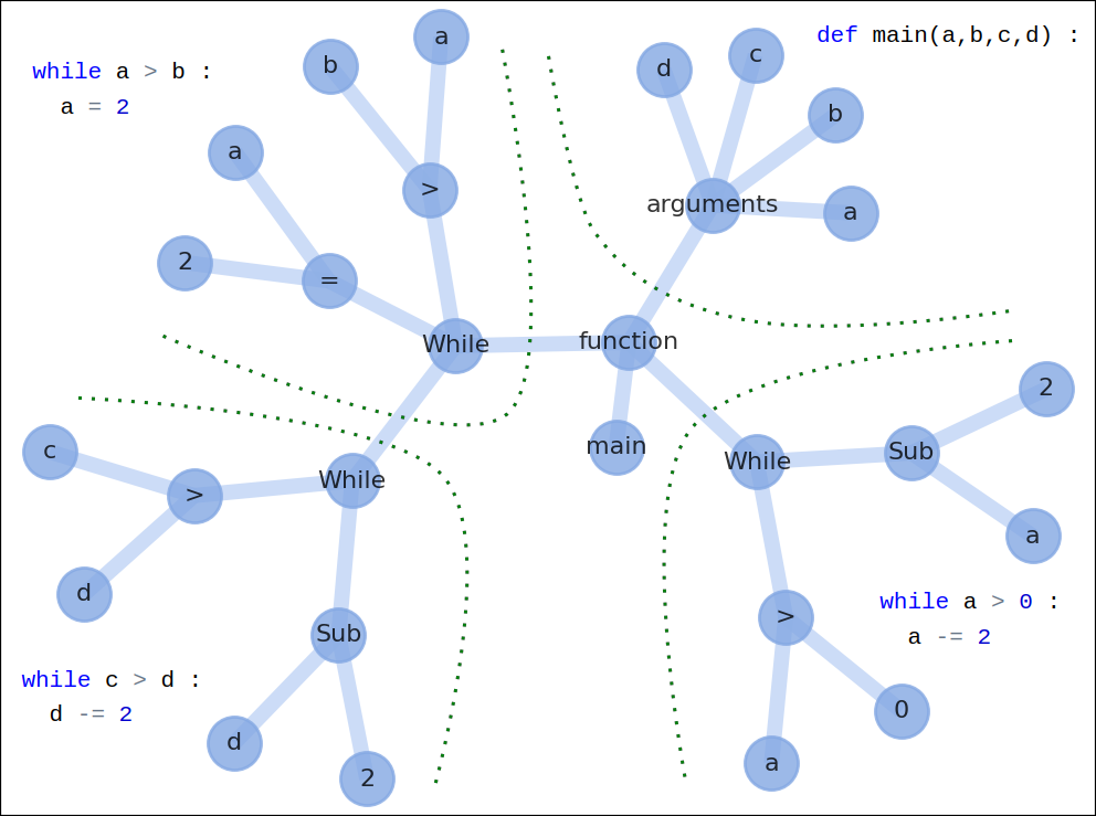
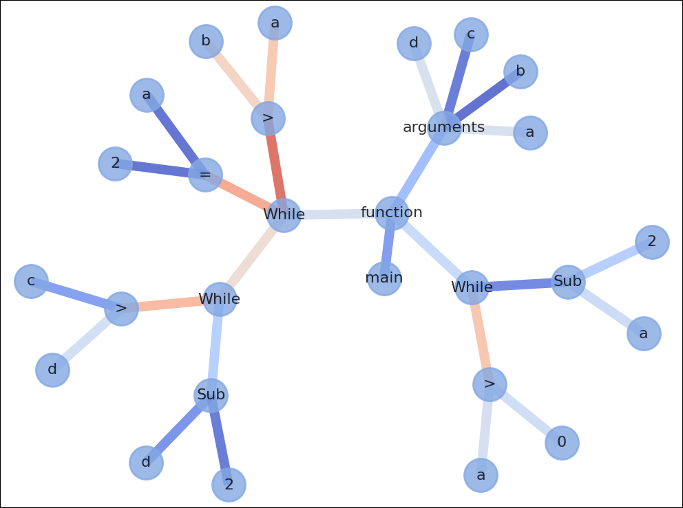
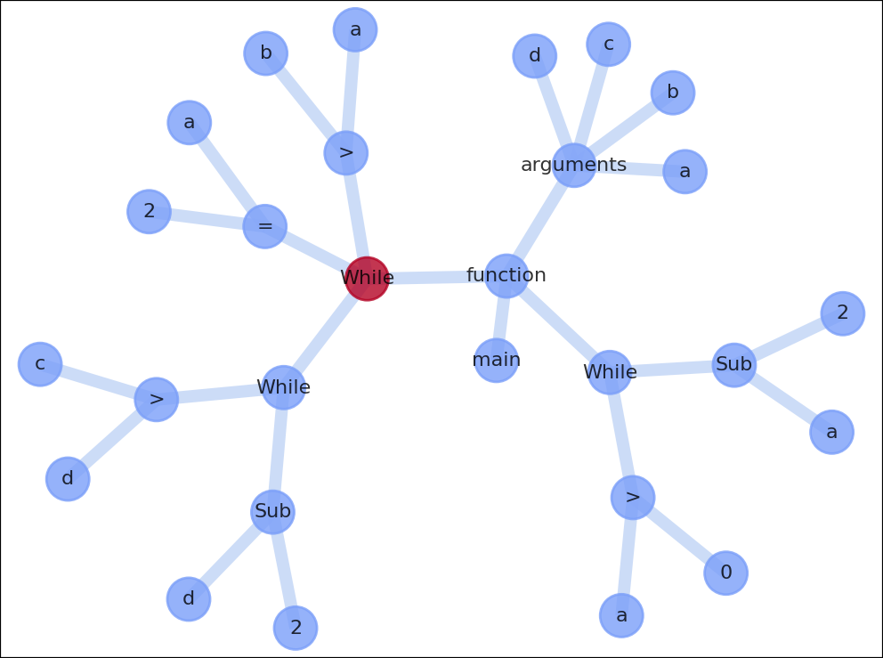
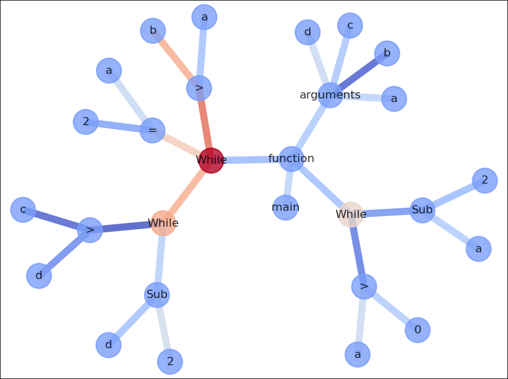
Figure 1. (a) AST (for clarity, we point out the corresponding lines of code). (b) Visualization of attention for binary classification as edge color from blue for low attention to red for high attention. The edges with high attention are those connecting the while nodes to their loop guards. Among these, the highest attention is given to the nonterminating outer loop. (c) Result of semantic segmentation, where the node corresponding to the outermost infinite loop is coloured in red. (d) Semantic segmentation visualized together with the attention extracted from the segmentation network. Best viewed in color.

3. Description of our technique

In this section, we provide details about our technique. At a high level, we first convert programs to feature graphs and then feed them into a GNN. We will describe each step, including the structure of the models for termination classification and semantic segmentation of the nodes responsible for nontermination.

3.1. Generation of feature graphs

There are many graph representations of a program. In this work, we start from the Abstract Syntax Tree (AST), which is a homogenous, undirected graph, where each node denotes a construct occurring in the program. We picked ASTs as the starting point because they are simple to understand and construct while containing all the necessary information for investigating a program’s termination. As future work, we may consider different graph representations of programs.

We start by generating the AST of each program in our datasets. Then, all ASTs are converted into feature graphs by converting each node to a local feature vector in local representation or ’one-hot’-encoding. For this purpose, all the nodes in the ASTs generated for each dataset are gathered in a dictionary. The dictionary holds each encoding as key with the instruction as value.

Running example

For illustration, we refer to our running example in Figure 3, which contains three loops. Out of them, the first outer loop is nonterminating for any initial value of $b$ less than 2 and of $a$ greater than $b$. Note that for machine integers (i.e. bit-vectors), the inner loop does terminate even when starting from a $c$ greater than $d$ because $d$ will eventually underflow, thus triggering a wrap-around behavior.

The running example is first converted to its AST as shown in Figure 1(a). Then, the AST is converted to the initial feature graph (before any convolutions). For reasons of space, we don’t show the whole feature graph, but rather just the subgraph corresponding to the instructions while c>d: d-=2 in Figure 2. The dictionary maps each node in the AST to a one-hot encoding. For instance, the while node is mapped to $0\cdots 00010000$. Similarly, both nodes corresponding to variable d have the same encoding, $0\cdots 00000010$. As we use the same dictionary for a whole dataset, identical nodes in the dataset will have the same encoding.

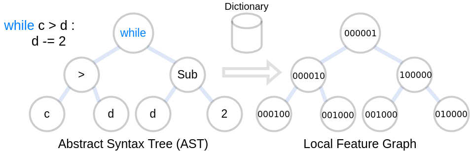
Figure 2. Conversion of an AST to a local feature graph (using ’one-hot’-encoding).

⬇

1 def main(a,b,c,d) :

2

3 while a > b:

4 a = 2

5 while c > d:

6 d -= 2

7

8 while a > 0:

9 a -= 2

Figure 3. Running example

3.2. Binary classification of termination based on GCN

For our first attempt at a binary classifier for program termination, we make use of GCN. In particular, we take inspiration from the architecture in (Kipf and Welling, 2016) in a supervised training setting. Currently, we do not train on recursive programs, where the nontermination could be caused by infinite recursion. We plan to do this as future work. For now, our datasets contain programs with potentially infinite loops.

Our termination classification is a graph level task, where we predict an attribute for the entire graph (in our case the termination behavior of the corresponding program) by aggregating all node features.

As explained in Section 2, GNNs use message passing to aggregate the information about a node’s neighbors to update the node’s value. According to (Kipf and Welling, 2016), we use:

(2) $$h_{i}^{(l+1)}=\sigma(b^{(l)}+\sum_{j\in N(i)}\frac{1}{c_{ij}}h_{j}^{(l)}W^{(l)})$$

where $c_{ij}=\sqrt{|N(i)|}\sqrt{|N(j)|}$, $N(i)$ describes the set of direct neighbours of $i$, and $\sigma$ is the activation function.

Best results are achieved using a rectified linear unit (ReLu) activation function. The weights $W^{(l)}$ are initialized using Glorot uniform and the bias $b$ with zero. The experiments of (Kipf and Welling, 2016) with other aggregation operators rather than the one used here, such as Multi-Layer-Perceptron aggregator (Zaheer et al., 2017) and Graph Attention Networks (Veličković et al., 2018), achieved similar results.

For the architecture in (Kipf and Welling, 2016), the graph convolution layers generate node-wise features. In our architecture, given that termination classification is a graph-level task, we choose to mean all the nodes once graph convolution is done and pass the resulting mean feature vector through three fully connected layers. Then, we apply a softmax function on the resulting two-dimensional vector to achieve a binary estimation. The resulting vector is then optimized by computing the cross-entropy loss with the ground truth.

Running example

For our running example in Figure 3, our classifier correctly concludes that the program is nonterminating. As aforementioned, we operate in a supervised training setting, meaning that our classifier has already been trained on the required dataset. We will give more details on the training and testing in Section 4.

3.3. Binary classification of termination based on GAT

If we revisit the update rule of GCNs given by Equation 2, it uses the coefficient $\frac{1}{c_{ij}}=\frac{1}{\sqrt{|N(i)|}\sqrt{|N(j)|}}$. Intuitively, this coefficient suggests the importance of node $j$’s features for node $i$ and it is heavily dependent on the structure of the graph (i.e. each node’s neighbours). The main idea of GATs (Veličković et al., 2018) is to compute this coefficient implicitly rather than explicitly as GCNs do by considering it to be a learnable attention mechanism. In the rest of the section, we refer to this coefficient as the attention score.

The main observation that led us to use GATs is the fact that not all instructions in a program are equally important when investigating its termination behavior. For instance, loops tend to be more important than straight-line code, and should therefore be given increased attention. Thus, our task naturally lends itself to using the attention mechanism. Moreover, our intention for this work is not only to design a program termination classifier but also to gain insights into its decisions. Using GATs helps us in this direction as it allows us to visualize those nodes that influence the decision related to termination.

Next, we explain next how the aggregation and update of node features $h_{i}^{(l)}$ to $h_{i}^{(l+1)}$ for iteration $l$ is derived. Initially, each node feature is passed through a simple linear layer by multiplying the feature with a learnable weight matrix $W^{(l)}$:

(3) $$z_{i}^{(l)}=W^{(l)}h_{i}^{(l)}$$

To obtain the pair-wise importance $e_{ij}^{(l)}$ of two neighbor features $h_{i}^{(l)}$ and $h_{j}^{(l)}$ we concatenate the previously computed embeddings $z_{i}^{(l)}$ and $z_{j}^{(l)}$ to $(z_{i}^{(l)}|z_{j}^{(l)})$. Then, the concatenated embeddings are fed into another linear layer with weight matrix $W_{2}^{(l)}$ that learns the attention scale $a^{(l)}$. Additionally, a leakyReLU activation function (Xu et al., 2015) is applied to introduce non-linearity:

(4) $$a^{(l)}=\text{LeakyReLU}(W^{(l)}(z_{i}^{(l)}|z_{j}^{(l)}))$$

After computation of $a$, corresponding to the activation scale, the pair-wise importance $e_{ij}^{(l)}$ of two neighbor features is:

(5) $$e_{ij}^{(l)}=\text{LeakyReLU}(\vec{a}^{(l)^{T}}(z_{i}^{(l)}|z_{j}^{(l)}))$$

As noted by (Veličković et al., 2018), the resulting attention scale can be considered as edge data. In our problem setting, this gives us insight into the importance of two connected syntax tree nodes with respect to the program’s termination.

To normalize the attention scores for all incoming edges we a apply a softmax layer:

(6) $$\alpha_{ij}^{(l)}=\frac{\exp(e_{ij}^{(l)})}{\sum_{k\in N(i)}\exp(e_{ik}^{(l)})}$$

Then, the neighbor embeddings are aggregated and scaled by the final attention scores $\alpha_{ij}^{(l)}$:

(7) $$h_{i}^{(l+1)}=\sigma\left(\sum_{j\in N(i)}{\alpha^{(l)}_{ij}z^{(l)}_{j}}\right)$$

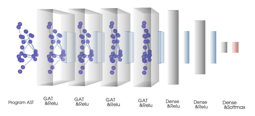
Figure 4. GAT-based architecture for the binary classification of program termination.

The architecture of our GAT-based termination classifier is shown in Figure 4 and includes multiple connected GAT layers with ReLu activation. Graph convolutions extract features to an intermediate representation, denoted by the last GAT layer with ReLu activation. Conversely to regular graph attention networks, we devise a prediction on the program’s termination by extracting the mean of node features and using dense layers with a final softmax layer. The attention information is extracted from the last GAT layer and can be associated with the AST edges.

Running example

Similar to the GCN, the GAT-based classifier identifies that the running example is nonterminating. Additionally, in Figure 1(b) we also obtain a visualization of edge-wise attention from blue for low attention to red for high attention. Notably, the edges with high attention are those connecting the while nodes to their loop guards. The extraction of attention gives us an intuition about which nodes have a high influence on the final prediction provided by the classifier. Although for this example, the edge connecting the nonterminating outer loop with its loop guard gets the highest attention, the difference between the attention scores linked to the three loops is not reliable enough to differentiate between the three loops and determine the cause for nontermination.

3.4. Semantic segmentation of nodes causing nontermination

While GATs provide some insight into the decision made by the classifier (by allowing us to visualize those AST nodes influencing the decision), we want to find the likely cause of nontermination. In particular, in this work, we try to localize the outermost infinitely looping constructs. Note that in the case where we have several nested loops and the outer one is infinitely looping, all of the inner ones will also be visited infinitely often. In such a situation, we identify the outer loop as the likely cause of nontermination, i.e. the outermost infinitely visited loop. As aforementioned, for now, we do not train on recursive programs, where the nontermination could be caused by infinite recursion. Thus, in our setting nontermination can only be caused by infinite loops.

Identifying the outermost infinitely visited loop is not possible with the information that we gained up until this point. Although in Figure 1(b), the edge between the nonterminating outer loop and its guard gets the highest attention, the edges connecting the other two loops and their guards also have high attention scores. Thus, it is hard to differentiate between the different loops based on the attention score alone.

To achieve our goal of identifying the outermost infinitely visited loop, we make use of semantic segmentation. Semantic segmentation has been primarily used in image recognition to label each pixel of an image with a particular class, allowing one to identify objects belonging to that class. Sometimes in the literature, the semantic segmentation of graphs is also named ’node-wise classification’ or ’node-classification’.

In this work, we attempt to extend the same principle that was applied in image recognition to programs by using semantic segmentation to identify those statements that cause nontermination. If we consider that program statements can belong to two classes, namely those that cause nontermination and those that don’t, we can envision that segmentation may help identify the former.

The graph network must convert feature vectors to an estimation. For this purpose, it is trained on the loss between ground truth and prediction on a node level. This can be accomplished with most segmentation loss functions such as a simple cross-entropy loss for binary segmentation with ground truth $y$ and prediction $\hat{y}$:

(8) $$L(y,\hat{y})=-(y\log(\hat{y})+(1-y)\log(1-\hat{y}))$$

Although the above loss enables the setup of an initial training session, it is not ideal to eradicate hard negatives. To improve and continue training beyond binary cross-entropy convergence, we use focal loss (Jadon, 2020; Lin et al., 2017), an extension of cross-entropy, which down-weights simple samples and gives additional weight to hard negatives:

(9) $$FL(p_{t})=-\alpha_{t}(1-p_{t})^{\gamma}log(p_{t})$$

with $\gamma,\alpha\in[0,1]$ and the modulation fact $(1-p_{t})^{\gamma}$, where $p_{t}=p$ for $y=1$ and $p_{t}=1-p$ otherwise.

Following the same message passing method explained in Section 3.2, the new node features hold the segmentation prediction.

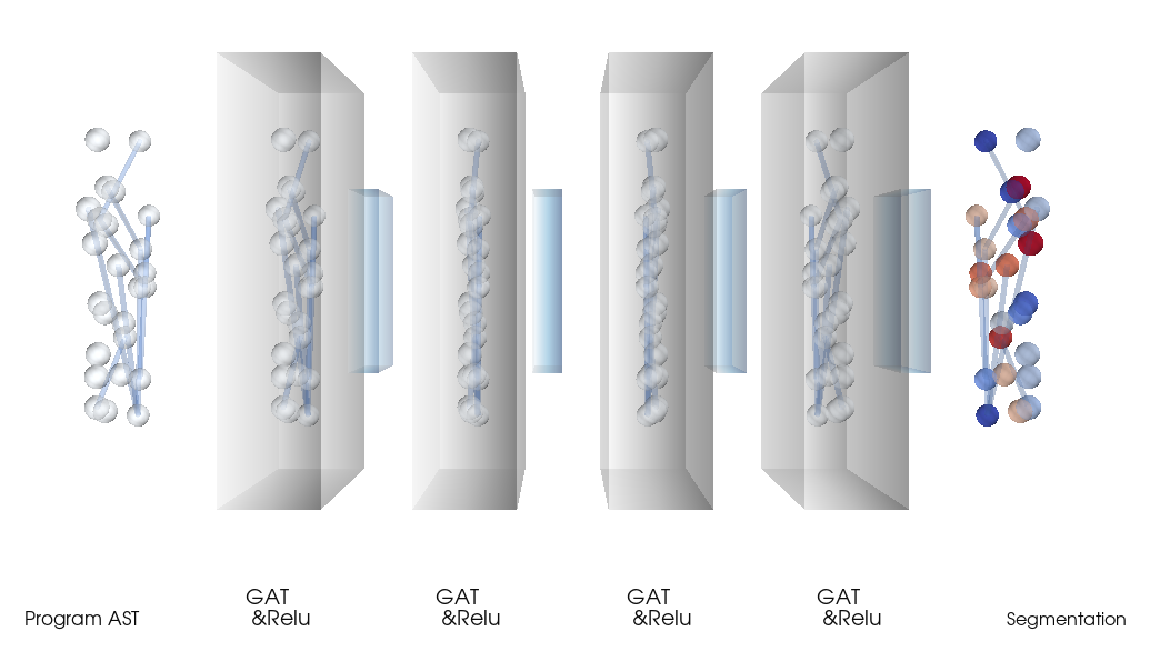
Figure 5. Proposed GAT-based architecture for the segmentation of nodes causing nontermination.

Our architecture for semantic segmentation is visualized in Figure 5. Graph attention convolution generates a semantic segmentation resulting in a node-wise estimation of likelihood to cause nontermination. By the attention mechanism, edge-wise scores denote the weight of features based on relational patterns.

Running example

The result of semantic segmentation for our running example is highlighted in Figure 1 (c), where the red-colored node denotes the outermost infinite loop. Figure 1 (d) shows the result of segmentation with attention.

3.5. Using the result of segmentation for debugging

One issue with the result of segmentation is that it only highlights the node corresponding to the head of the outermost nonterminating loop, rather than all the statements contributing to nontermination. This is obvious for our running example in Figure 1 (c), where segmentation only identifies the node corresponding to the nonterminating while loop.

This was a conscious decision on our part, meant to simplify the construction of the required training datasets. While there are a huge number of programs available online, it’s not at all straightforward to use them for training machine learning-based techniques for program analysis. The main reason for this is that such programs are not labeled with the result of any analysis, and manually labeling them is difficult and error-prone. In particular, for the termination classification task, we must know which programs are terminating and which are not. Even more problematic, for semantic segmentation, the annotation should, in principle, identify all the instructions contributing to nontermination. For instance, for our running example, it should identify lines 3 and 4. In general, it can be very difficult to annotate such datasets.

In this work, to simplify the annotation for segmentation, we only label the node corresponding to the head of the outermost infinite loop as the reason for nontermination. More details on the way we generate our datasets are given in Section 4.

While identifying the outermost infinite loop is already useful, debugging can be further aided by finding the rest of the instructions that contribute to nontermination. This can be achieved with slicing (Weiser, 1982). In general, slicing is a program analysis technique that aims to extract parts of a program according to a particular slicing criterion (e.g. it can extract instructions responsible for the write accesses to a particular variable). In our scenario, given a nonterminating loop returned by segmentation, we can use several slicing criteria in order to isolate the faulty loop, while preserving the nontermination behavior highlighted by segmentation. One option, which we illustrate below on the running example in Figure 3, is a criterion aiming to preserve the reachability of a control flow point (in particular, we are interested in the control flow point at the entrance to the nonterminating loop). Among other tools, such a slicing capability is provided by the software analysis platform Frama-C (Baudin et al., 2021). Other slicing criteria can be used, e.g. preserving the values of the variables used by the guard of the infinite loop. Slicing has been previously used in the context of debugging nontermination, e.g. failure-slices in (Neumerkel and Mesnard, 1999).

Going back to our running example in Figure 3, once segmentation has identified the first outer loop as the likely culprit for nontermination, we slice the program such that we preserve the reachability of the control flow point at the entrance to the body of the nonterminating outer loop. This gives us the program in Figure 6. This sliced program preserves the nontermination behavior of the original program (induced by the loop identified by segmentation) while cutting down the syntactic structure, which corresponds to reducing its state space.

Intuitively, cutting down the state space of the program makes it more amenable to other existing debugging techniques such as fuzzing. For illustration, we have asked libFuzzer (lib, [n. d.]) (a library for coverage-guided fuzz testing) to search for an input that triggers execution of the sliced program longer than 5s. LibFuzzer was able to find the input $a$ = 165017090 and $b$ = -183891446 within 6s. This input triggers the nontermination behavior and can assist in further debugging. Conversely, when asking libFuzzer to find such input for the original in Figure 3, it required 12s. We expect the difference between the two running times to increase for larger programs.

Overall, the debugging workflow that we envision follows the following steps: (1) our classifier estimates that a program is nonterminating; (2) our technique based on GNNs and semantic segmentation finds the likely root cause of nontermination; (3) slicing cuts down the syntactic structure of the program and implicitly its state space, while aiming to maintain the faulty nontermination behavior; (4) fuzzing finds faulty inputs for the sliced program.

If a program contains several nontermination bugs, the debugging workflow above may need to be repeated until all of the bugs are eliminated.

⬇

1 def main(a,b) :

2 while a > b:

3 a = 2

Figure 6. Nonterminating slice of the running example

4. Experiments

4.1. System

For our experiments, we used the deep learning framework PyTorch (Paszke et al., 2017) with the GNN package DGL (Deep Graph Library) and various packages for preprocessing and visualization. The experiments were performed using an RTX 2080 8GB GPU on a local machine. The architecture of the GNNs used, depending on the particular experiment consists of between 4 and 6 graph layers. While this is typical for the effective training of GNNs, it could be extended using residual blocks (Li et al., 2019).

4.2. Binary classification of program termination

We start by discussing our experimental evaluation for the binary classification of program termination. Given a program, our classifier extracts a termination estimation, i.e. whether the program is terminating or nonterminating. Concerning the latter, a program is considered nonterminating if there exists an input for which the program’s execution is infinite.

4.2.1. Classification datasets

Our experiments on classification and semantic segmentation of the cause for nontermination require different datasets. This is because classification data requires program-level annotations (a program is labeled as terminating or nonterminating), whereas segmentation requires node-wise annotations (each node in the AST is either a cause for nontermination or not). In this section, we discuss the datasets used for classification, whereas more details on those used for segmentation can be found in Section 4.3.1.

For classification, we use a total of four datasets, out of which two are based on existing benchmarks and two are generated by us. Concerning the datasets containing existing benchmarks, the first one, DS-SV-COMP, contains C programs from the termination category of the SV-COMP 2022 competition (sv-, 2022; Beyer, 2020). In particular, this dataset contains all programs from the following subcategories: termination-crafted, termination-crafted-lit, termination-numeric, and termination-restricted-15. In total, there are 55 nonterminating programs and 194 terminating. For a total of 249 programs, we count a total of 386 loops with a maximum of five nested loops for the program NO_04.c. The second dataset of existing benchmarks, DS-TERM-COMP, contains 150 C programs from the Termination Competition (Giesl et al., 2015) with a total of 452 loops and a maximum of 2 nested loops per program. These benchmarks are selected such that there is no overlap with those in the DS-SV-COMP dataset.

The benchmarks in both DS-SV-COMP and DS-TERM-COMP expect inputs meaning that their termination behavior depends on non-deterministic values. These benchmarks come already labeled as terminating or nonterminating, where the nontermination label indicates that there exists an input for which the program’s execution doesn’t terminate. The pre-processing of the datasets includes the generation of the AST representation for each program and the conversion to a feature graph using DGL.

For efficiency reasons, we consider batches of 30 graphs using the $dgl{.}batch$. The two datasets have an associated dictionary featuring all the distinct AST nodes from all the programs. Intuitively, this dictionary gives us the vocabulary used by the benchmarks. For more details on the generation of feature graphs, see Section 3.1.

As previously discussed in Section 3.5, one of the main challenges of our work is the fact that, while there are many available programs, only a few are already labeled as terminating or nonterminating (as we could see above, even existing software verification competitions only consider a relatively small number of benchmarks). However, machine learning techniques generally require large training data, which is not available in our setting. Due to this, we chose to also generate our additional custom datasets. For the first custom dataset, DS1, we used the dictionary generated for DS-SV-COMP and DS-TERM-COMP, meaning that the vocabulary of DS1 is the same as that of DS-SV-COMP and DS-TERM-COMP. This is important as it allows us to train on DS1 and only use DS-SV-COMP and DS-TERM-COMP for testing. DS1 contains 950 C programs. The second custom dataset, DS2, contains 950 generated Python programs, out of which 800 are used for training and 150 for testing.

To label the benchmarks in DS1 and DS2, we fuzz test for nontermination by generating a large number of inputs for each program. If the execution time reaches a predefined timeout for at least one of the inputs, then we label the program as nonterminating. The dataset is balanced by providing an equal number of terminating and nonterminating samples.

Apart from DS-SV-COMP and DS-TERM-COMP, each dataset is split into training and test samples by the general rule of approximately 80/20 depending on the dataset size. The exact split for each set is specified in Table 1.

Dataset	Origin	Language	Experiment	Training samples	Test samples
DS-SV-COMP	SV-Comp	C	classification	-	249
DS-TERM-COMP	TermComp	C	classification	-	150
DS1	custom	C	classification	800	150
DS2	custom	Python	classification	800	150
DS-Seg-Py1	custom	Python	semantic segmentation	180	50
DS-Seg-C	custom	C	semantic segmentation	180	50

Table 1. Datasets used in this work.

4.2.2. Training

As explained in Section 3, we deploy two different neural networks, one based on GCN (Kipf and Welling, 2016) and another one based on GAT (Veličković et al., 2018). In our experiments, we found that a number of 4 layers was sufficient for both the GCN and GAT architectures, respectively. Training is performed using an Adam-optimizer with an initial learning rate of 0.0001. We use a regular cross-entropy loss function and record various metrics such as the Receiver Operating Characteristic (ROC) curve and the Precision-Recall during training both for validation and testing.

For a significant evaluation, we perform a total of ten training sessions until convergence of the test metrics.

4.2.3. Results and evaluation

To judge the performance of our classifier, we use the Precision-Recall (PR) and Receiver Operating Characteristic (ROC) and their respective Area Under the Curve (AUC) and Average Precision (AP). AUC takes values from 0 to 1, where value 0 indicates a perfectly inaccurate test and 1 reflects a perfectly accurate test.

PR is used as an indication for the tradeoff between precision and recall for different thresholds. Consequently, high recall and high precision reflect in a high area under the curve. High precision is based on a low rate of false positives and a high recall is based on a low rate of false negatives.

The ROC curve plots the true positive rate versus the false positive rate for each threshold. The closer to the top-left corner a ROC curve is, the better, and the diagonal line corresponds to random guessing. A high area under the curve indicates a better classification performance.

The results of the experimental evaluation of our classifier are summarized in Table 2, where we record the AUC for positive (terminating) instances, the AUC for negative (nonterminating) instances, and the mean Average Precision (mAP), which is calculated as the average of the AP for terminating and nonterminating instances.

The first and arguably most important observation is that, with values of over 0.82 for all mAPs for both PR and ROC, we can conclude that classification results are significant and that we achieve a high ability to generalize for unknown data.

The second remark refers to the comparison of GCN and GAT. As observed in Table 2, the PR and ROC mAP numbers are generally higher for GAT than GCN, suggesting that the application of graph attention improves the result of the binary classification (we use bold font for the higher mAP numbers). This indicates that the applied self-attention mechanism does assign a higher weight to patterns responsible for deciding the termination behavior.

The third comparison we are interested in is between the classification of terminating and nonterminating programs. We notice that the PR AUC negative tends to be higher than AUC positive, meaning that the classifier performs better at identifying nonterminating programs. We conjecture that nonterminating patterns are easier to identify based on relational probabilistic patterns that are likely to cause nontermination.

In Figure 7 we visualize the ROC curves per class and layer type. The better performance for nontermination classes is reflected in higher red curves while the better performance of GAT layers is represented by higher continuous lines compared to doted CGN curves.

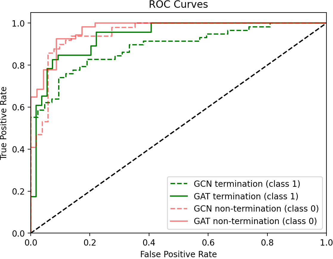
Figure 7. ROC curves per class (class 0 corresponds to nonterminating programs and class 1 to terminating ones) and experimental configuration.

4.3. Semantic segmentation of nodes causing nontermination

In this section, we describe our experiments for identifying the outermost nonterminating node using semantic segmentation.

4.3.1. Segmentation datasets

Several reasons prevent us from reusing the same benchmarks from DS-SV-COMP and DS-TERM-COMP for semantic segmentation. Firstly, they only contain a program-level label denoting whether the program terminates. For semantic segmentation, we require node-level annotations that indicate whether the corresponding AST node is likely to cause nontermination or not. Secondly, it is often very difficult to determine the cause for nontermination in existing benchmarks, as it isn’t labeled.

For this reason, we generate two datasets that consist only of nonterminating samples (as we would only attempt to find the cause for nontermination for those programs that were deemed nonterminating by our classifier). As explained in Section 3.5, we restrict our annotations to only identify the outermost nonterminating loop in the program. Note that if there are several distinct, outermost, nonterminating loops, only one of them will be labeled as causing nontermination. The reason for this is the fact that we use fuzz testing to determine the culpable loop, and we stop the fuzzing once we found the first nonterminating scenario. We use label 0 to indicate that the corresponding AST node has no relation to nontermination, and label 1 to indicate a high likelihood of causing nontermination.

The two datasets are described in the last two rows of Table 1. The first, DS-SegPy1 contains Python programs, whereas the second, DS-Seg-C, contains C programs. Each dataset is composed of 180 programs for training and 50 for testing. The program sample generator for custom data is probabilistic and generates programs that contain from two to five loops that can be nested.

4.3.2. Training

To improve and continue training beyond binary cross-entropy convergence, we deployed a focal loss (Jadon, 2020; Lin et al., 2017), an extension of cross-entropy that down-weights simple samples and gives additional weight to hard negatives.

To achieve optimal results, the experiments required modifying the learning rate, optimizer, network structure, and the number of features compared to those used for classification. The final configuration features an Adam optimizer with a learning rate of 0.001. In our experiments, we found that a number of 4 layers was sufficient for both the GCN and GAT architectures, respectively. While the GCN and GAT architectures used for semantic segmentation are respectively similar to those used for classification, they do not contain a node mean function and linear layers. The last GCN/GAT layer projects to a one-dimensional feature indicating the confidence that a node is causing nontermination.

Similar to the experiments for classification, we perform a total of ten training sessions until convergence of the test metrics.

4.3.3. Results and evaluation

The metrics used for evaluation are Jaccard loss based on intersection over union (IoU), the related Dice-Coefficient, and node-wise accuracy. A comprehensive overview of these metrics is provided by (Hossin and M.N, 2015). Similar to image segmentation where the pixel-wise accuracy is determined, here the node-wise distinction of true-positives, true-negatives, false-positives, and false-negatives for the node prediction compared to the annotated node ground truth is used.

We calculate the mean metrics for an average of 10 models that were trained to a convergence of validation scores for each experimental configuration. In the evaluation, we provide mean values with standard deviation.

From the results for semantic segmentation (detailed in Table 3) we can infer several observations. With mean values of more than 0.84 for Dice and IoU and a node accuracy of 0.81 in all experimental validation sets, the ability to generalize for unknown programs is high. The low standard deviation indicates a robust result for the state of convergence of validation metrics.

For dataset Seg-Py1 the mean Dice-Coefficient is higher for the GAT architecture by 3.3 percent than for GCN. Similarly, node accuracy is better by 4.7 percent with only a decrease of 0.8 percent for the IoU. This indicates an improvement in segmentation performance for GAT compared to GCN. Similarly, for C programs using dataset Seg-C, all metrics improved significantly with a 5 percent better performance for Dice-Coefficient and node accuracy and an increase of 12 percent for IoU. From the comparative better performance of GAT-layers for node-wise segmentation, we infer that the use of self-attention mechanisms enables the network to weigh more relevant node transitions and therefore achieve better performance. Higher attention is assigned to edges with a high likelihood of causing nontermination.

4.4. Comparison to recurrent algorithms

In Section 1, we discussed the suitability of GNNs for analyzing programs given the inherent graph structure of programs. The objective of the current section is to justify this statement by evaluating whether GNNs are better at estimating program termination than recurrent algorithms. Note that the latter are based on a sequential program representation.

For this purpose, we create an additional set of experiments for the binary classification of program termination. To make the comparison fair, the experimental configuration ensures that the number of learnable parameters of all recurrent algorithms is higher than the learnable parameters of the GNNs they were compared against. We use the PyTorch implementations for RNNs (Sherstinsky, 2018), Long short-term memory (LSTM) (Hochreiter and Schmidhuber, 1997) and Gated recurrent unit’s (GRU) (Chung et al., 2014).

For this experiment, we only use the DS2 dataset containing Python programs. Conversely to the previous experiments, for the recurrent algorithms, the programs are not converted into an AST but are directly encoded into a one-hot encoding based on a dictionary of unique instructions.

For a significant evaluation, we perform a total of ten training sessions until convergence of the test metrics.

4.4.1. Results

Similar to the previous classification experiments we record the Precision-Recall (PR) and Receiver Operating Characteristic (ROC) and their respective AUC.

We summarize our experimental results in Table 4. Notably, graph-based methods outperform recurrent approaches by more than 5 percent for the best recurrent ROC-AUC and PR-AUC metrics. Intuitively, we infer that the graph representation of programs is a better fit for termination estimation than the sequential representation. Furthermore, the understanding of the context within the recurrent networks is limited by the model capacity and by the natural constraints that don’t allow for large sequences of data to be processed.

Additional insight into the comparison of the classification results can be gained by examining Figure 8, where it can be observed that the GNN and GAT-based architectures perform better than the recurrent approaches.

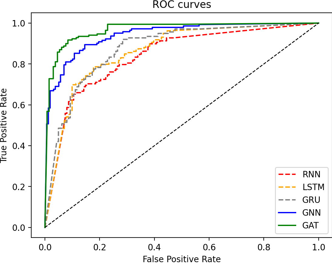
Figure 8. Binary classification for termination in recurrent and graph neural networks. The graph neural network based approaches perform significantly better than classical recurrent approaches.

	Precision-Recall				ROC
Approach	Dataset	mAP	AUC negative	AUC positive	mAP	AUC neg.	AUC pos.
GCN	DS-SV-COMP	0.83	0.94	0.76	0.87	0.88	0.88
	DS-TERM-COMP	0.87	0.92	0.84	0.90	0.89	0.89
	DS1	0.92	0.94	0.90	0.93	0.92	0.92
	DS2	0.87	0.91	0.88	0.91	0.91	0.91
GAT	DS-SV-COMP	0.9	0.96	0.86	0.93	0.93	0.93
	DS-TERM-COMP	0.91	0.93	0.89	0.92	0.91	0.91
	DS1	0.93	0.91	0.74	0.93	0.94	0.93
	DS2	0.90	0.94	0.88	0.92	0.93	0.93

Table 2. Experimental results for the binary classification of program termination using different network architectures and datasets. ROC and Precision-Recall are recorded after a test accuracy convergence.

			Dice-Coefficient		Jaccard Index (IoU)		Node Accuracy
Approach	Dataset	Language	value	$\sigma$	value	$\sigma$	value	$\sigma$
GCN	Seg-Py1	Python	0.843	0.021	0.856	0.029	0.810	0.026
	Seg-C	C	0.896	0.031	0.812	0.029	0.892	0.034
GAT	Seg-Py1	Python	0.876	0.020	0.848	0.024	0.857	0.023
	Seg-C	C	0.947	0.012	0.943	0.024	0.944	0.013

Table 3. Experimental results for the semantic segmentation of termination using different network architectures and datasets.

Approach	Network	ROC-AUC	PR-AUC
recurrent	RNN (Sherstinsky, 2018)	0.78	0.77
	LSTM (Hochreiter and Schmidhuber, 1997)	0.88	0.87
	GRU (Chung et al., 2014)	0.88	0.88
graph based	GCN (custom)	0.94	0.94
	GAT (custom)	0.96	0.96

Table 4. Experimental comparison of binary classification using RNNs vs. GNNs.

5. Related Work

5.1. Termination analysis

Termination analysis has been studied for a long time. While the majority of the approaches make use of symbolic methods such as loop summarisation (Chen et al., 2018a; Zhu and Kincaid, 2021), program synthesis (Fedyukovich et al., 2018; David et al., 2015), quantifier elimination (Le et al., 2018), abstract interpretation (Cousot and Cousot, 2012), there were recent attempts to employ machine learning techniques.

For instance, Neural Termination Analysis (Giacobbe et al., 2021b), trains neural networks as ranking functions, i.e. monotone maps from the program’s state space to well-ordered sets.

This method uses sampled executions to learn ranking functions, which are then verified with an SMT solver. Several limitations exist for this approach, e.g. loops with a limited number of iterations do not provide enough data to learn a ranking function, the verification of the ranking function may require additional loop invariants to succeed. Moreover, this work has only been evaluated on terminating programs with a maximum of two nested loops. Calude and Dumitrescu proposed a probabilistic algorithm for the Halting problem based on running times, where they define a class of computable probability distributions on the set of halting programs (Calude and Dumitrescu, 2017). In (Abate et al., 2021b), Abate et al. present the first machine learning approach to the termination analysis of probabilistic programs, where they use a neural network to fit a ranking supermartingales over execution traces and then verify it over the source code with an SMT solver.

As opposed to these existing works, we do not attempt to provide strong guarantees about the termination decision. Instead, our objective is to provide an estimation of a program’s termination behavior, as well as localizing the likely cause of nontermination (when applicable) that a programmer can use for debugging purposes. For this purpose, we employ the attention mechanism to identify those nodes relevant for the termination estimation. Moreover, for programs classified as nonterminating, we use semantic segmentation to distinguish the outermost loop causing the infinite execution.

5.2. Graph Neural Networks

The original approach to GNNs as presented by Kipf and Welling (Kipf and Welling, 2016) used the sum of normalized neighbor embeddings as aggregation in a self-loop. With a Multi-Layer-Perceptron as an aggregator, Zaheer et al. (Zaheer et al., 2017) presented an approach that propagates states through a trainable MLP. With the development of advanced attention networks, the approach of Velickovic et al. (Veličković et al., 2018) focused on attention weights that allow to prioritize the influence of features based on self-learned attention. For heterogeneous graphs with additional edge features, Relational Graph Convolution Networks were introduced by Schlichtkrull et. al. (Schlichtkrull et al., 2018) to enable link prediction and entity classification, allowing the recovery of missing entity attributes for high-dimensional knowledge graphs.

6. Conclusions

We proposed a technique for estimating the termination behavior of programs using a GNN. We also devised a GAT architecture that uses a self-attention mechanism to allow the visualization of nodes relevant for the termination decision. Finally, for nonterminating programs, we constructed a GAT for the semantic segmentation of those nodes likely responsible for nontermination.

Experimental evaluation of our algorithm confirms a superior performance in termination estimation with a high ability to generalize for unknown programs.

References

- (1)
- lib ([n. d.]) [n. d.]. https://llvm.org/docs/LibFuzzer.html
- sv- (2022) 2022. Competition on Software Verification. https://sv-comp.sosy-lab.org/2022/
- Abate et al. (2021a) Alessandro Abate, Mirco Giacobbe, and Diptarko Roy. 2021a. Learning Probabilistic Termination Proofs. 3–26. https://doi.org/10.1007/978-3-030-81688-9_1
- Abate et al. (2021b) Alessandro Abate, Mirco Giacobbe, and Diptarko Roy. 2021b. Learning Probabilistic Termination Proofs. In Computer Aided Verification - 33rd International Conference, CAV 2021, Virtual Event, July 20-23, 2021, Proceedings, Part II (Lecture Notes in Computer Science, Vol. 12760), Alexandra Silva and K. Rustan M. Leino (Eds.). Springer, 3–26. https://doi.org/10.1007/978-3-030-81688-9_1
- Alias et al. (2010) Christophe Alias, Alain Darte, Paul Feautrier, and Laure Gonnord. 2010. Multi-dimensional rankings, program termination, and complexity bounds of flowchart programs. In International Static Analysis Symposium. Springer, 117–133.
- Alias et al. (2013) C. Alias, A. Darte, P. Feautrier, and L. Gonnord. 2013. Rank: A Tool to Check Program Termination and Computational Complexity. In 2013 IEEE Sixth International Conference on Software Testing, Verification and Validation Workshops. 238–238. https://doi.org/10.1109/ICSTW.2013.75
- Allamanis ([n. d.]) Miltiadis Allamanis. [n. d.]. Graph Neural Networks on Program Analysis. ([n. d.]).
- Allamanis et al. (2017) Miltiadis Allamanis, Marc Brockschmidt, and Mahmoud Khademi. 2017. Learning to Represent Programs with Graphs. CoRR abs/1711.00740 (2017). arXiv:1711.00740 http://arxiv.org/abs/1711.00740
- Allamanis et al. (2021) Miltiadis Allamanis, Henry Jackson-Flux, and Marc Brockschmidt. 2021. Self-Supervised Bug Detection and Repair. CoRR abs/2105.12787 (2021). arXiv:2105.12787 https://arxiv.org/abs/2105.12787
- Baudin et al. (2021) Patrick Baudin, François Bobot, David Bühler, Loïc Correnson, Florent Kirchner, Nikolai Kosmatov, André Maroneze, Valentin Perrelle, Virgile Prevosto, Julien Signoles, and Nicky Williams. 2021. The dogged pursuit of bug-free C programs: the Frama-C software analysis platform. Commun. ACM 64, 8 (2021), 56–68. https://doi.org/10.1145/3470569
- Ben-Amram and Genaim (2012) Amir M. Ben-Amram and Samir Genaim. 2012. On the Linear Ranking Problem for Integer Linear-Constraint Loops. CoRR abs/1208.4041 (2012). arXiv:1208.4041 http://arxiv.org/abs/1208.4041
- Beyer (2020) Dirk Beyer. 2020. Advances in Automatic Software Verification: SV-COMP 2020. In Tools and Algorithms for the Construction and Analysis of Systems, Armin Biere and David Parker (Eds.). Springer International Publishing, Cham, 347–367.
- Bieber et al. (2020) David Bieber, Charles Sutton, Hugo Larochelle, and Daniel Tarlow. 2020. Learning to execute programs with instruction pointer attention graph neural networks. arXiv preprint arXiv:2010.12621 (2020).
- Calude and Dumitrescu (2017) Cristian Calude and Monica Dumitrescu. 2017. A probabilistic anytime algorithm for the halting problem. Computability 7 (05 2017), 1–13. https://doi.org/10.3233/COM-170073
- Chatterjee et al. (2021) Krishnendu Chatterjee, Ehsan Kafshdar Goharshady, Petr Novotný, and Dorde Zikelic. 2021. Proving non-termination by program reversal. In PLDI ’21: 42nd ACM SIGPLAN International Conference on Programming Language Design and Implementation, Virtual Event, Canada, June 20-25, 20211, Stephen N. Freund and Eran Yahav (Eds.). ACM, 1033–1048. https://doi.org/10.1145/3453483.3454093
- Chen et al. (2018a) Hong-Yi Chen, Cristina David, Daniel Kroening, Peter Schrammel, and Björn Wachter. 2018a. Bit-Precise Procedure-Modular Termination Analysis. ACM Trans. Program. Lang. Syst. 40, 1 (2018), 1:1–1:38. https://doi.org/10.1145/3121136
- Chen et al. (2009) Wei Chen, Tie-Yan Liu, Yanyan Lan, Zhiming Ma, and Hang Li. 2009. Ranking Measures and Loss Functions in Learning to Rank. 315–323.
- Chen et al. (2018b) Yu-Fang Chen, Matthias Heizmann, Ondřej Lengál, Yong Li, Ming-Hsien Tsai, Andrea Turrini, and Lijun Zhang. 2018b. Advanced automata-based algorithms for program termination checking. In Proceedings of the 39th ACM SIGPLAN Conference on Programming Language Design and Implementation. 135–150.
- Chung et al. (2014) Junyoung Chung, Çaglar Gülçehre, KyungHyun Cho, and Yoshua Bengio. 2014. Empirical Evaluation of Gated Recurrent Neural Networks on Sequence Modeling. CoRR abs/1412.3555 (2014). arXiv:1412.3555 http://arxiv.org/abs/1412.3555
- Colón and Sipma (2002) Michael A Colón and Henny B Sipma. 2002. Practical methods for proving program termination. In International Conference on Computer Aided Verification. Springer, 442–454.
- Cook (2009) Byron Cook. 2009. Priciples of program termination. Engineering Methods and Tools for Software Safety and Security 22, 161 (2009), 125.
- Cook et al. (2006) Byron Cook, Andreas Podelski, and Andrey Rybalchenko. 2006. Termination proofs for systems code. In Proceedings of the ACM SIGPLAN 2006 Conference on Programming Language Design and Implementation, Ottawa, Ontario, Canada, June 11-14, 2006, Michael I. Schwartzbach and Thomas Ball (Eds.). ACM, 415–426. https://doi.org/10.1145/1133981.1134029
- Cook et al. (2013) Byron Cook, Abigail See, and Florian Zuleger. 2013. Ramsey vs. Lexicographic Termination Proving. In Tools and Algorithms for the Construction and Analysis of Systems - 19th International Conference, TACAS 2013, Held as Part of the European Joint Conferences on Theory and Practice of Software, ETAPS 2013, Rome, Italy, March 16-24, 2013. Proceedings (Lecture Notes in Computer Science, Vol. 7795), Nir Piterman and Scott A. Smolka (Eds.). Springer, 47–61. https://doi.org/10.1007/978-3-642-36742-7_4
- Cousot and Cousot (2012) Patrick Cousot and Radhia Cousot. 2012. An abstract interpretation framework for termination. In Proceedings of the 39th ACM SIGPLAN-SIGACT Symposium on Principles of Programming Languages, POPL 2012, Philadelphia, Pennsylvania, USA, January 22-28, 2012, John Field and Michael Hicks (Eds.). ACM, 245–258. https://doi.org/10.1145/2103656.2103687
- David et al. (2015) Cristina David, Daniel Kroening, and Matt Lewis. 2015. Unrestricted Termination and Non-termination Arguments for Bit-Vector Programs. In Programming Languages and Systems - 24th European Symposium on Programming, ESOP 2015, Held as Part of the European Joint Conferences on Theory and Practice of Software, ETAPS 2015, London, UK, April 11-18, 2015. Proceedings (Lecture Notes in Computer Science, Vol. 9032), Jan Vitek (Ed.). Springer, 183–204. https://doi.org/10.1007/978-3-662-46669-8_8
- Dwivedi et al. (2020) Vijay Prakash Dwivedi, Chaitanya K Joshi, Thomas Laurent, Yoshua Bengio, and Xavier Bresson. 2020. Benchmarking graph neural networks. arXiv preprint arXiv:2003.00982 (2020).
- Fedyukovich et al. (2018) Grigory Fedyukovich, Yueling Zhang, and Aarti Gupta. 2018. Syntax-Guided Termination Analysis. In Computer Aided Verification - 30th International Conference, CAV 2018, Held as Part of the Federated Logic Conference, FloC 2018, Oxford, UK, July 14-17, 2018, Proceedings, Part I (Lecture Notes in Computer Science, Vol. 10981), Hana Chockler and Georg Weissenbacher (Eds.). Springer, 124–143. https://doi.org/10.1007/978-3-319-96145-3_7
- Giacobbe et al. (2021a) Mirco Giacobbe, Mohammadhosein Hasanbeig, Daniel Kroening, and Hjalmar Wijk. 2021a. Shielding Atari Games with Bounded Prescience. CoRR abs/2101.08153 (2021). arXiv:2101.08153 https://arxiv.org/abs/2101.08153
- Giacobbe et al. (2021b) Mirco Giacobbe, Daniel Kroening, and Julian Parsert. 2021b. Neural Termination Analysis. arXiv:2102.03824 [cs.LG]
- Giesl et al. (2017) Jürgen Giesl, Cornelius Aschermann, Marc Brockschmidt, Fabian Emmes, Florian Frohn, Carsten Fuhs, Jera Hensel, Carsten Otto, Martin Plücker, Peter Schneider-Kamp, et al. 2017. Analyzing program termination and complexity automatically with AProVE. Journal of Automated Reasoning 58, 1 (2017), 3–31.
- Giesl et al. (2015) Jürgen Giesl, Fred Mesnard, Albert Rubio, René Thiemann, and Johannes Waldmann. 2015. Termination Competition (termCOMP 2015). https://doi.org/10.1007/978-3-319-21401-6_6
- Grohe (2021) Martin Grohe. 2021. The Logic of Graph Neural Networks. CoRR abs/2104.14624 (2021). arXiv:2104.14624 https://arxiv.org/abs/2104.14624
- Gupta et al. (2008) Ashutosh Gupta, Thomas A. Henzinger, Rupak Majumdar, Andrey Rybalchenko, and Ru-Gang Xu. 2008. Proving non-termination. In Proceedings of the 35th ACM SIGPLAN-SIGACT Symposium on Principles of Programming Languages, POPL 2008, San Francisco, California, USA, January 7-12, 2008, George C. Necula and Philip Wadler (Eds.). ACM, 147–158. https://doi.org/10.1145/1328438.1328459
- Hamaguchi et al. (2017) Takuo Hamaguchi, Hidekazu Oiwa, Masashi Shimbo, and Yuji Matsumoto. 2017. Knowledge transfer for out-of-knowledge-base entities: A graph neural network approach. arXiv preprint arXiv:1706.05674 (2017).
- Heizmann et al. (2013) Matthias Heizmann, Jochen Hoenicke, and Andreas Podelski. 2013. Software Model Checking for People Who Love Automata. In Computer Aided Verification - 25th International Conference, CAV 2013, Saint Petersburg, Russia, July 13-19, 2013. Proceedings (Lecture Notes in Computer Science, Vol. 8044), Natasha Sharygina and Helmut Veith (Eds.). Springer, 36–52. https://doi.org/10.1007/978-3-642-39799-8_2
- Heizmann et al. (2014) Matthias Heizmann, Jochen Hoenicke, and Andreas Podelski. 2014. Termination Analysis by Learning Terminating Programs. https://doi.org/10.1007/978-3-319-08867-9_53
- Hochreiter and Schmidhuber (1997) Sepp Hochreiter and Jürgen Schmidhuber. 1997. Long Short-term Memory. Neural computation 9 (12 1997), 1735–80. https://doi.org/10.1162/neco.1997.9.8.1735
- Hossin and M.N (2015) Mohammad Hossin and Sulaiman M.N. 2015. A Review on Evaluation Metrics for Data Classification Evaluations. International Journal of Data Mining & Knowledge Management Process 5 (03 2015), 01–11. https://doi.org/10.5121/ijdkp.2015.5201
- Jadon (2020) Shruti Jadon. 2020. A survey of loss functions for semantic segmentation. 2020 IEEE Conference on Computational Intelligence in Bioinformatics and Computational Biology (CIBCB) (Oct 2020). https://doi.org/10.1109/cibcb48159.2020.9277638
- Kipf and Welling (2016) Thomas N. Kipf and Max Welling. 2016. Semi-Supervised Classification with Graph Convolutional Networks. CoRR abs/1609.02907 (2016). arXiv:1609.02907 http://arxiv.org/abs/1609.02907
- Le et al. (2016) Tien-Duy B. Le, David Lo, Claire Le Goues, and Lars Grunske. 2016. A learning-to-rank based fault localization approach using likely invariants. In Proceedings of the 25th International Symposium on Software Testing and Analysis, ISSTA 2016, Saarbrücken, Germany, July 18-20, 2016, Andreas Zeller and Abhik Roychoudhury (Eds.). ACM, 177–188. https://doi.org/10.1145/2931037.2931049
- Le et al. (2018) Ton Chanh Le, Lei Xu, Lin Chen, and Weidong Shi. 2018. Proving Conditional Termination for Smart Contracts. In Proceedings of the 2nd ACM Workshop on Blockchains, Cryptocurrencies, and Contracts, BCC@AsiaCCS 2018, Incheon, Republic of Korea, June 4, 2018, Satya V. Lokam, Sushmita Ruj, and Kouichi Sakurai (Eds.). ACM, 57–59. https://doi.org/10.1145/3205230.3205239
- Lee et al. (2001) Chin Soon Lee, Neil D Jones, and Amir M Ben-Amram. 2001. The size-change principle for program termination. In Proceedings of the 28th ACM SIGPLAN-SIGACT symposium on Principles of programming languages. 81–92.
- Li et al. (2019) Guohao Li, Matthias Müller, Guocheng Qian, Itzel C. Delgadillo, Abdulellah Abualshour, Ali K. Thabet, and Bernard Ghanem. 2019. DeepGCNs: Making GCNs Go as Deep as CNNs. CoRR abs/1910.06849 (2019). arXiv:1910.06849 http://arxiv.org/abs/1910.06849
- Li et al. (2018) Jun Li, Bodong Zhao, and Chao Zhang. 2018. Fuzzing: a survey. Cybersecurity 1 (12 2018). https://doi.org/10.1186/s42400-018-0002-y
- Lin et al. (2017) Tsung-Yi Lin, Priya Goyal, Ross Girshick, Kaiming He, and Piotr Dollár. 2017. Focal loss for dense object detection. In Proceedings of the IEEE international conference on computer vision. 2980–2988.
- Liu et al. (2020a) Meng Liu, Hongyang Gao, and Shuiwang Ji. 2020a. Towards deeper graph neural networks. In Proceedings of the 26th ACM SIGKDD International Conference on Knowledge Discovery and Data Mining. 338–348.
- Liu et al. (2020b) Qinghui Liu, Michael Kampffmeyer, Robert Jenssen, and Arnt-Børre Salberg. 2020b. SCG-Net: Self-Constructing Graph Neural Networks for Semantic Segmentation. CoRR abs/2009.01599 (2020). arXiv:2009.01599 https://arxiv.org/abs/2009.01599
- Manès et al. (2018) Valentin J. M. Manès, HyungSeok Han, Choongwoo Han, Sang Kil Cha, Manuel Egele, Edward J. Schwartz, and Maverick Woo. 2018. Fuzzing: Art, Science, and Engineering. CoRR abs/1812.00140 (2018). arXiv:1812.00140 http://arxiv.org/abs/1812.00140
- Nair et al. (2020) Aravind Nair, Avijit Roy, and Karl Meinke. 2020. funcGNN: A Graph Neural Network Approach to Program Similarity. CoRR abs/2007.13239 (2020). arXiv:2007.13239 https://arxiv.org/abs/2007.13239
- Neumerkel and Mesnard (1999) Ulrich Neumerkel and Frédéric Mesnard. 1999. Localizing and Explaining Reasons for Non-terminating Logic Programs with Failure-Slices. In Principles and Practice of Declarative Programming, International Conference PPDP’99, Paris, France, September 29 - October 1, 1999, Proceedings (Lecture Notes in Computer Science, Vol. 1702), Gopalan Nadathur (Ed.). Springer, 328–342. https://doi.org/10.1007/10704567_20
- Paszke et al. (2017) Adam Paszke, Sam Gross, Soumith Chintala, Gregory Chanan, Edward Yang, Zachary DeVito, Zeming Lin, Alban Desmaison, Luca Antiga, and Adam Lerer. 2017. Automatic differentiation in PyTorch. In NIPS-W.
- Sanchez-Gonzalez et al. (2018) Alvaro Sanchez-Gonzalez, Nicolas Heess, Jost Tobias Springenberg, Josh Merel, Martin Riedmiller, Raia Hadsell, and Peter Battaglia. 2018. Graph networks as learnable physics engines for inference and control. In International Conference on Machine Learning. PMLR, 4470–4479.
- Sasirekha et al. (2011) N. Sasirekha, A. Edwin Robert, and M. Hemalatha. 2011. Program slicing techniques and its applications. CoRR abs/1108.1352 (2011). arXiv:1108.1352 http://arxiv.org/abs/1108.1352
- Scarselli et al. (2008) Franco Scarselli, Marco Gori, Ah Chung Tsoi, Markus Hagenbuchner, and Gabriele Monfardini. 2008. Computational capabilities of graph neural networks. IEEE Transactions on Neural Networks 20, 1 (2008), 81–102.
- Schlichtkrull et al. (2018) M. Schlichtkrull, Thomas Kipf, P. Bloem, Rianne van den Berg, Ivan Titov, and M. Welling. 2018. Modeling Relational Data with Graph Convolutional Networks. In ESWC.
- Sherstinsky (2018) Alex Sherstinsky. 2018. Fundamentals of Recurrent Neural Network (RNN) and Long Short-Term Memory (LSTM) Network. CoRR abs/1808.03314 (2018). arXiv:1808.03314 http://arxiv.org/abs/1808.03314
- Shi and Rajkumar (2020) Weijing Shi and Ragunathan Rajkumar. 2020. Point-GNN: Graph Neural Network for 3D Object Detection in a Point Cloud. CoRR abs/2003.01251 (2020). arXiv:2003.01251 https://arxiv.org/abs/2003.01251
- Si et al. (2018) X. Si, H. Dai, Mukund Raghothaman, M. Naik, and Le Song. 2018. Learning Loop Invariants for Program Verification. In NeurIPS.
- Turing (1936) Alan Turing. 1936. On Computable Numbers, with an Application to the N Tscheidungsproblem. Proceedings of the London Mathematical Society 42, 1 (1936), 230–265. https://doi.org/10.2307/2268810
- Veličković et al. (2018) Petar Veličković, Guillem Cucurull, Arantxa Casanova, Adriana Romero, Pietro Liò, and Yoshua Bengio. 2018. Graph Attention Networks. arXiv:1710.10903 [stat.ML]
- Wei et al. (2020) Jiayi Wei, Maruth Goyal, Greg Durrett, and Isil Dillig. 2020. LambdaNet: Probabilistic Type Inference using Graph Neural Networks. CoRR abs/2005.02161 (2020). arXiv:2005.02161 https://arxiv.org/abs/2005.02161
- Weiser (1982) Mark Weiser. 1982. Programmers Use Slices When Debugging. Commun. ACM 25, 7 (jul 1982), 446–452. https://doi.org/10.1145/358557.358577
- Weiser (1984) Mark Weiser. 1984. Program Slicing. IEEE Transactions on Software Engineering SE-10, 4 (1984), 352–357. https://doi.org/10.1109/TSE.1984.5010248
- Wu et al. (2020) Yongji Wu, Defu Lian, Yiheng Xu, Le Wu, and Enhong Chen. 2020. Graph Convolutional Networks with Markov Random Field Reasoning for Social Spammer Detection. In The Thirty-Fourth AAAI Conference on Artificial Intelligence, AAAI 2020, The Thirty-Second Innovative Applications of Artificial Intelligence Conference, IAAI 2020, The Tenth AAAI Symposium on Educational Advances in Artificial Intelligence, EAAI 2020, New York, NY, USA, February 7-12, 2020. AAAI Press, 1054–1061. https://aaai.org/ojs/index.php/AAAI/article/view/5455
- Wu et al. (2019) Zonghan Wu, Shirui Pan, Fengwen Chen, Guodong Long, Chengqi Zhang, and Philip S. Yu. 2019. A Comprehensive Survey on Graph Neural Networks. CoRR abs/1901.00596 (2019). arXiv:1901.00596 http://arxiv.org/abs/1901.00596
- Xi (2002) Hongwei Xi. 2002. Dependent types for program termination verification. Higher-Order and Symbolic Computation 15, 1 (2002), 91–131.
- Xu et al. (2015) Bing Xu, Naiyan Wang, Tianqi Chen, and Mu Li. 2015. Empirical Evaluation of Rectified Activations in Convolutional Network. CoRR abs/1505.00853 (2015). arXiv:1505.00853 http://arxiv.org/abs/1505.00853
- Xu et al. (2018) Keyulu Xu, Weihua Hu, Jure Leskovec, and Stefanie Jegelka. 2018. How powerful are graph neural networks? arXiv preprint arXiv:1810.00826 (2018).
- Zaheer et al. (2017) Manzil Zaheer, Satwik Kottur, Siamak Ravanbakhsh, Barnabás Póczos, Ruslan Salakhutdinov, and Alexander J. Smola. 2017. Deep Sets. CoRR abs/1703.06114 (2017). arXiv:1703.06114 http://arxiv.org/abs/1703.06114
- Zhang and Rabbat (2018) Yingxue Zhang and Michael G. Rabbat. 2018. A Graph-CNN for 3D Point Cloud Classification. CoRR abs/1812.01711 (2018). arXiv:1812.01711 http://arxiv.org/abs/1812.01711
- Zhang et al. (2018) Ziwei Zhang, Peng Cui, and Wenwu Zhu. 2018. Deep Learning on Graphs: A Survey. CoRR abs/1812.04202 (2018). arXiv:1812.04202 http://arxiv.org/abs/1812.04202
- Zhou et al. (2020) Jie Zhou, Ganqu Cui, Shengding Hu, Zhengyan Zhang, Cheng Yang, Zhiyuan Liu, Lifeng Wang, Changcheng Li, and Maosong Sun. 2020. Graph neural networks: A review of methods and applications. AI Open 1 (2020), 57–81. https://doi.org/10.1016/j.aiopen.2021.01.001
- Zhu and Kincaid (2021) Shaowei Zhu and Zachary Kincaid. 2021. Termination analysis without the tears. In PLDI ’21: 42nd ACM SIGPLAN International Conference on Programming Language Design and Implementation, Virtual Event, Canada, June 20-25, 2021, Stephen N. Freund and Eran Yahav (Eds.). ACM, 1296–1311. https://doi.org/10.1145/3453483.3454110