Relativistic Bohmian trajectories and Klein-Gordon currents for spin-0 particles

Abstract

It is generally believed that the de Broglie-Bohm model does not admit a particle interpretation for massive relativistic spin-0 particles, on the basis that particle trajectories cannot be defined. We show this situation is due to the fact that in the standard (canonical) representation of the Klein-Gordon equation the wavefunction systematically contains superpositions of particle and anti-particle contributions. We argue that by working in a Foldy-Wouthuysen type representation uncoupling the particle from the anti-particle evolutions, a positive conserved density for a particle and associated density current can be defined. For the free Klein-Gordon equation the velocity field obtained from this current density appears to be well-behaved and sub-luminal in typical instances. As an illustration, Bohmian trajectories for a spin-0 boson distribution are computed numerically for free propagation in situations in which the standard velocity field would take arbitrarily high positive and negative values.

I Introduction

The de Broglie-Bohm interpretation of quantum mechanics dB ; bohm has played and still plays an important role in our understanding of quantum mechanics. Not that one should necessarily endorse the ontological package and mechanisms put forward by the Bohmian model as describing the “real” behavior of quantum systems. The strength of the Bohmian model lies, in our view, elsewhere: by proposing an account of dynamical processes for which the orthodox interpretation tells us we should give up any attempt to explain them, the de Broglie-Bohm interpretation improves our understanding and our intuition of quantum phenomena.

However, this situation holds for non-relativistic quantum mechanics based on the Schrödinger equation. In the relativistic domain, the Bohmian model suffers from several difficulties. In particular, it seems impossible, to define trajectories for spin-0 bosons described by the Klein-Gordon equation (see Ch. 11 of Ref. undivided ). Obviously, one might expect that in the high-energy regimes in which particles can be created or destroyed, the usual Bohmian framework based on continuous trajectories would need to be replaced by a different picture based on quantum field theory. But it might appear surprising that even in low energy regimes, it is not possible to give a de Broglie-Bohm trajectory description of a spin-0 particle propagating in free space.

The aim of this work is to examine the underlying reasons for the breakdown of the Bohmian model for systems obeying the Klein Gordon equation, point out how the problems can be repaired, and effectively introduce Bohmian trajectories from a newly defined Klein-Gordon current. In a nutshell, our view is that in relativistic quantum mechanics, a quantum state intrinsically superposes particles and anti-particles. In particular, causality only holds if the time evolution operator includes the propagator for the particle and anti-particle sectors. So a generic state describing a particle (with a positive density everywhere) will develop anti-particle components, and the density will become negative in some spatial regions. This leads to superluminal velocities and closed loops in space-time dewd , a feature that is deemed "inconsistent" (see Sec. 10.4 of Ref. undivided , or holland-PR ) with the guidance formula at the basis of the Bohmian model. This is why in the past some radical solutions have been proposed, such as restricting the set of admissible states to those that lead to positive only densities kypra , or employing the absolute value of the density in order to define trajectories nikolic08 . The first solution does not work, as remarked by Bell (see footnote in kypra ), while the second one still leads to superluminal velocities for the Bohmian particle. Other approaches have also been suggested vigier-H ; dewdney2000 ; holland2019 ; vollick2021 .

The solution we will advocate will be to work in a representation that uncouples the particle and anti-particle sectors. In momentum space, this is well-known to be possible through Foldy-Wouthuysen-type transformations FW ; case ; FV (see also silenko for a recent review). Then a new density needs to be defined in this representation. A locally conserved current different from the canonical one can indeed be defined in a given reference frame, though it is known that such currents do not transform as a 4-vector hoffmann .

We will begin (Sec. 2) by recalling how the Bohmian velocity field naturally appears in non-relativistic quantum mechanics, even without imposing the guidance formula. We will then examine why the same procedure does not work with the Klein-Gordon equation in its canonical form. In Sec. 3 we will introduce the representation separating the particle and anti-particle sectors and introduce the density and corresponding current defined directly in that representation. We will then define de Broglie-Bohm trajectories in that representation and compute trajectories for the free Klein-Gordon equation (Sec. 4). We close with a few concluding remarks (Sec. 5).

II Density current and particle velocity

II.1 Non-relativistic guidance equation

In the usual non-relativistic de Broglie-Bohm approach, the particle velocity $v_{j}(x,t)$ is obtained from the standard Schrödinger current $j_{NR}(x,t)$ through

$$v_{j}(x,t)=\frac{j_{NR}(x,t)}{\rho_{NR}(x,t)}$$ (1)

where

$$\rho_{NR}(x,t)=\left|\left\langle x\right|\left.\psi\right\rangle\right|^{2}$$ (2)

is the probability density, whose conservation takes the form

$$\frac{\partial\rho_{NR}}{\partial t}+\partial_{x}j_{NR}(x,t)=0$$ (3)

(to simplify the notation, we will assume a free Hamiltonian and stay in one spatial dimension). Recall that $v_{j}(x,t)$ defines a velocity field, and that the Bohmian particle follows the streamlines of the current: the trajectory $x(t)$ is obtained by integrating the guidance equation

$$\frac{dx}{dt}=v_{j}\left(x(t),t\right)$$ (4)

with an initial condition $x(t_{0})=x_{0}$.

The current can be written as the symmetrized combination of the momentum operator $P$ and a spatial projection:

$$j_{NR}(x,t)=\frac{1}{2m}\left(\left\langle\psi\right|P\left|x\right\rangle\left\langle x\right|\left.\psi\right\rangle+\left\langle\psi\right|\left.x\right\rangle\left\langle x\right|P\left|\psi\right\rangle\right),$$ (5)

and the average of the current density is easily seen to yield

$$\left\langle j_{NR}(t)\right\rangle=\int dxj_{NR}(x,t)=\left\langle\psi\right|\frac{P}{m}\left|\psi\right\rangle\equiv\left\langle\psi\right|V\left|\psi\right\rangle$$ (6)

where $V\equiv P/m$ can be seen as a velocity operator. Hence the average Schrödinger current gives the average velocity of the system.

It is also straightforward to write Eq. (5) as

$$j_{NR}(x,t)=\left|\left\langle x\right|\left.\psi\right\rangle\right|^{2}\left[\frac{1}{2}\left(\frac{\left\langle\psi\right|\frac{P}{m}\left|x\right\rangle}{\left\langle\psi\right|\left.x\right\rangle}+\frac{\left\langle x\right|\frac{P}{m}\left|\psi\right\rangle}{\left\langle x\right|\left.\psi\right\rangle}\right)\right].$$ (7)

Comparing with Eqs. (1) and (2), we see that the term between $[...]$ is precisely the velocity (1) that we can rewrite as

$$v_{j}(x,t)=\operatorname{Re}\frac{\left\langle x\right|V\left|\psi\right\rangle}{\left\langle x\right|\left.\psi\right\rangle}.$$ (8)

The expression on the right handside is sometimes known as the weak value of the velocity operator . The important point is that the velocity of the particle in the non-relativistic de Broglie-Bohm approach is naturally defined from the wavefunction and the velocity operator.

II.2 Klein-Gordon equation

II.2.1 Current and density in the canonical formulation

The Klein-Gordon equation in its usual “canonical” form is greiner

$$(i\hbar\partial_{t})^{2}\psi=\left(P^{2}c^{2}+m^{2}c^{4}\right)\psi$$ (9)

and the associated density reads

$$\rho(x,t)=\frac{i\hbar}{2mc^{2}}\left(\psi^{\ast}(x,t)\partial_{t}\psi(x,t)-\psi(x,t)\partial_{t}\psi^{\ast}(x,t)\right);$$ (10)

$m$ is the rest mass and $c$ the light velocity and the $\partial_{t}$ term entering the definition of the scalar product is due to the presence of a second order time derivative in Eq. (9). The density is not positive definite (this will become clearer below), and $\rho$ is therefore interpreted as a charge density. Note that in the free case plane waves with both positive and negative energies are solutions of Eq. (9), associated with particles and anti-particles respectively greiner .

The corresponding conserved current obeying $\partial_{t}\rho+\partial_{x}j=0$ can be written in the same form as the Schrödinger current (5), namely

$$j(x,t)=\frac{1}{2m}\left(\left\langle\psi\right|P\left|x\right\rangle\left\langle x\right|\left.\psi\right\rangle+\left\langle\psi\right|\left.x\right\rangle\left\langle x\right|P\left|\psi\right\rangle\right).$$ (11)

We therefore also have as for the Schrödinger current average

$$\left\langle j(t)\right\rangle=\left\langle\psi\right|\frac{P}{m}\left|\psi\right\rangle.$$ (12)

But in a relativistic context, $p/m$ is not the classical velocity of a particle (it is not even bounded); the classical expression for the relativistic velocity is

$$v_{cl}=\frac{pc^{2}}{E_{p}}=\frac{p}{\gamma m},$$ (13)

where $E_{p}\equiv\sqrt{p^{2}c^{2}+m^{2}c^{4}}$. Hence there is no analog for the right hand-side of Eq. (6). Moreover the current cannot take the form (7), as $\left|\left\langle x\right|\left.\psi\right\rangle\right|^{2}$ does not represent the conserved density.

II.2.2 Klein-Gordon equation in Hamilton form

As is well-known greiner , the Klein-Gordon (KG) equation can be written in a form involving a first order time derivative,

$$i\hbar\partial_{t}\Psi=\left[\left(\tau_{3}+i\tau_{2}\right)\frac{P^{2}}{2m}+\tau_{3}mc^{2}\right]\Psi$$ (14)

where $\tau_{i}$ are the usual Pauli matrices (generally denoted $\sigma_{i}$ in other contexts). The wave-function

$$\Psi=\left(\begin{array}[c]{c}\varphi\\ \chi\end{array}\right)$$ (15)

is now a 2-dimensional vector whose components are related to the solutions of the canonical KG equation (9) by

$$\psi =\varphi+\chi$$ (16)

$$i\hbar\partial_{t}\psi =mc^{2}\left(\varphi-\chi\right).$$ (17)

The positive and negative energy plane-wave solutions of the canonical KG equation become

$$\Psi^{+} =\frac{1}{2\sqrt{mc^{2}E_{p}}}\left(\begin{array}[c]{c}mc^{2}+E_{p}\\ mc^{2}-E_{p}\end{array}\right)e^{-i\left(E_{p}t-px\right)/\hbar}$$ (20)

$$\Psi^{-} =\frac{1}{2\sqrt{mc^{2}E_{p}}}\left(\begin{array}[c]{c}mc^{2}-E_{p}\\ mc^{2}+E_{p}\end{array}\right)e^{i\left(E_{p}t-px\right)/\hbar}.$$ (23)

The density (10) and current (11) take the form

$$\rho =\left\langle\Psi\right|\tau_{3}\left|x\right\rangle\left\langle x\right|\left.\Psi\right\rangle=\left|\varphi(x)\right|^{2}-\left|\chi(x)\right|^{2}$$ (24)

$$j =\frac{1}{2}\left(\left\langle\Psi\right|\tau_{3}\left|x\right\rangle\left\langle x\right|\left(\tau_{3}+i\tau_{2}\right)\frac{P}{m}\left|\Psi\right\rangle+\left\langle\Psi\right|\tau_{3}\left(\tau_{3}+i\tau_{2}\right)\frac{P}{m}\left|x\right\rangle\left\langle x\right|\left.\Psi\right\rangle\right)$$ (25)

Note that the right hand-side of Eq. (24) indicates that $\chi(x)$ contributes to a negative charge and can thus be seen as an anti-particle contribution. The $\tau_{3}$ matrix in the dual vector is the signature of the pseudo-Hermitian character of the KG formalism  mosta , the (non-positively defined) inner product being given by $\left\langle\Psi_{1}\right|\left.\Psi_{2}\right\rangle_{KG}=\left\langle\Psi_{1}\right|\tau_{3}\left|\Psi_{2}\right\rangle.$ The momentum operator is multiplied by $\tau_{3}+i\tau_{2},$ changing the sign of the anti-particle contribution.

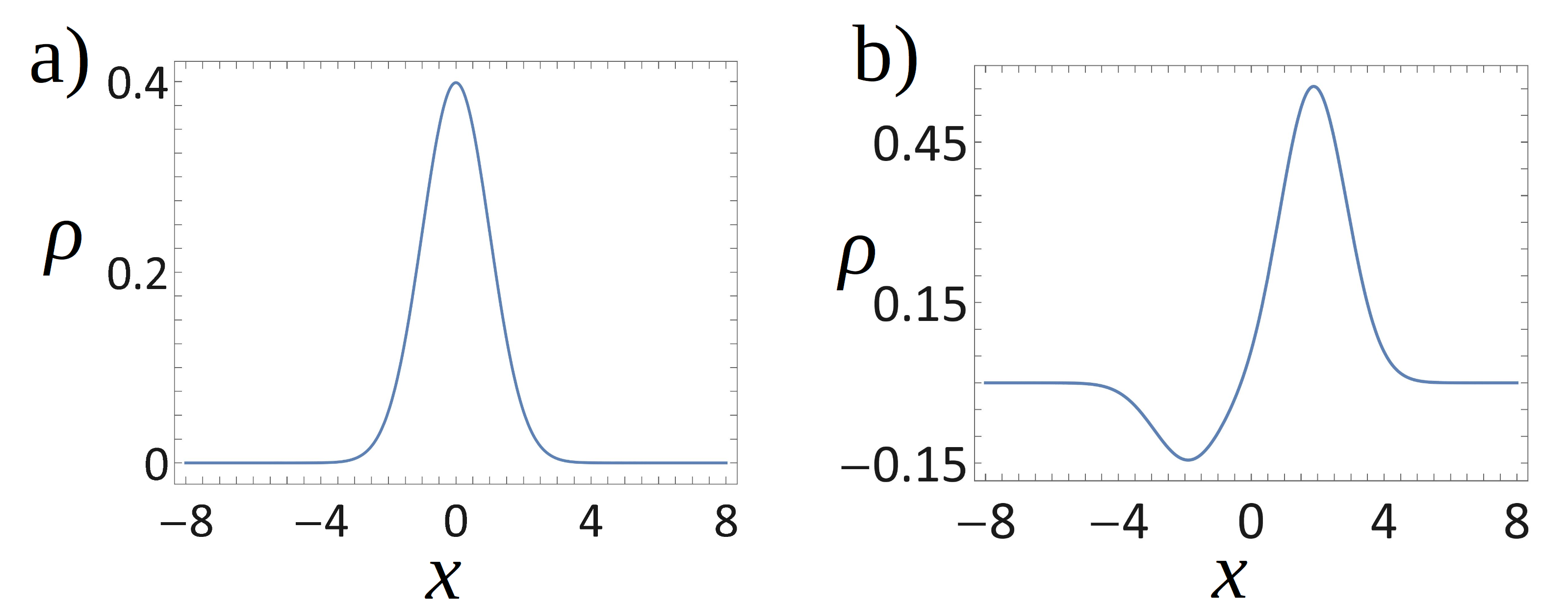
Figure 1: The canonical Klein-Gordon density $\rho(x,t)$ of an ultra-relativistic spin-0 boson (a) at $t=0$ and (b) at $t=2$ (natural units $\hbar=c=m=1$ are used). At $t=0$ the distribution is a Gaussian (with mean momentum $p_{0}=3$, mean position $x_{0}=0$ and unit spatial width) that is everywhere positive, but the density becomes negative in some regions as the wavefunction evolves.

II.2.3 Standard Bohmian particle velocity

The Hamiltonian formulation of the KG equation – a system of two coupled linear equations – is handy in showing that a normalized initial state $\Psi(t_{0},x)=\left(\begin{array}[c]{c}\varphi(t_{0},x)\\ 0\end{array}\right)$ with positive charge $\rho=\left|\varphi(t_{0},x)\right|^{2}$ everywhere at $t=t_{0}$ will become at an evolved time $\Psi(t,x)=\left(\begin{array}[c]{c}\varphi(t,x)\\ \chi(t,x)\end{array}\right),$ so that typically $\rho(t,x)$  will become negative in some regions. Attempting to define a Bohmian velocity through

$$v(t,x)\overset{?}{=}\frac{j(t,x)}{\rho(t,x)}$$ (26)

will lead to regions of infinitely high velocities. This happens in the vicinity of a point for which $\rho(t,x)=0,$ but this does not necessarily imply that $j(x)\rightarrow 0$. Indeed, according to Eq. (24), an equal amount of positive and negative charge yields a vanishing density, i.e. $\left|\varphi(x)\right|\rightarrow\left|\chi(x)\right|\Longrightarrow\rho(x)\rightarrow 0$.

An illustration is given in Fig. 1: an initial positive charged Gaussian (Fig. 1(a)) quickly develops regions of negative charge density (Fig. 1(b)). The velocity field, as defined by Eq. (26) is shown in Fig. 2. Regions of superluminal velocities are readily visible, as expected when $\rho(t,x)$ goes through 0 and changes sign. The wavefunctions were computed semi-analytically from the wavepacket expansion of the time-evolved Gaussian in the Hamiltonian representation (see mak for details).

While it is generally acknowledged that having a superluminal motion ruins a particle trajectory interpretation of spin-0 bosons undivided ; dewd ; holland-book , some authors, beginning with de Broglie debroglie-KGsup (see also nikolic04 ) have asserted that this type of motion is not a problem as long as it does not have experimental consequences (that is, this type of behavior for individual particles is washed out by the intrinsically statistical nature of the quantum formalism). One of us has argued elsewhere pitfall ; billiard on general grounds why, if the de Broglie-Bohm interpretation is taken as a realist construal of quantum phenomena, such arguments should be rejected, as they undermine realism (since any fundamental dynamical law can be postulated as long as the statistical predictions are recovered) and employ the same type of strategy as the Copenhagen interpretation: what matters in the predictive agreement with experiments, and an experiment that would specifically measure velocities will never detect superluminal aspects . For this reason, in our view a particle interpretation for spin-0 bosons hinges on the existence of well-behaved trajectories.

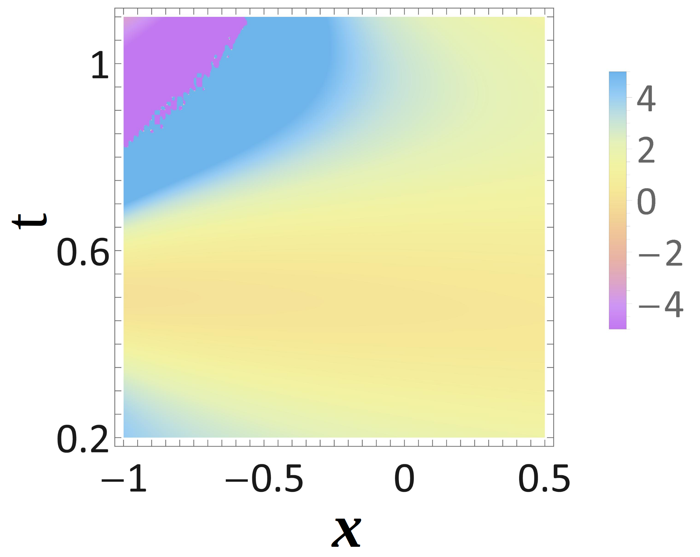
Figure 2: The velocity field defined by Eq. (26) in a given space-time region for the initial density shown in Fig. 1(a) (natural units are used). The velocity field is superluminal in some spatial regions.

III Separating particles from anti-particles

III.1 Pseudo-unitary transformations

Representations decoupling the positive and energy components were looked for soon after the classic Newton-Wigner work NW on the correct form of the position operator in relativistic quantum mechanics. This was first worked out in the context of the Dirac equation by Foldy and Wouthuysen FW , and then generalized to the Klein-Gordon case and particles of arbitrary spin case ; FV . It was indeed realized costella ; silenko that the representation in which $X$ is the position operator is not the standard Dirac one, nor in the KG case the Hamilton formulation given by Eq. (14), but a representation in which the particle and anti-particle components are not coupled.

The unitary transformation (or rather, pseudo-unitary in the KG case) depends on the specific Hamiltonian of the problem. It is known in explicit form in a few special cases, including the free Hamiltonian. For the free particle KG Hamiltonian (14), a well-known operator greiner that separates particles from anti-particles is

$$U=\frac{\left(mc^{2}+E_{p}\right)-\tau_{1}\left(mc^{2}-E_{p}\right)}{\sqrt{4mc^{2}E_{p}}}.$$ (27)

Note that $U$ is pseudo-unitary in the sense that $U^{\dagger}\neq U^{-1}$ but $\tau_{3}U^{\dagger}\tau_{3}=U^{-1}$. The positive and negative energy solutions (20) and (23) become

$$\Phi^{+}(p,t) =U\Psi^{+}=\left(\begin{array}[c]{c}1\\ 0\end{array}\right)e^{-i\left(E_{p}t-px\right)/\hbar}$$ (30)

$$\Phi^{-}(p,t) =U\Psi^{-}=\left(\begin{array}[c]{c}0\\ 1\end{array}\right)e^{i\left(E_{p}t-px\right)/\hbar}.$$ (33)

$\Phi^{+}(p,t)$ defines indeed a state with pure particle contribution. The KG equation (14) becomes

$$i\hbar\partial_{t}\Phi=H_{\Phi}\Phi$$ (34)

with

$$H_{\Phi}=UHU^{-1}=\tau_{3}\sqrt{p^{2}c^{2}+m^{2}c^{4}},$$ (35)

Since the Hamiltonian in this representation – which, contrary to Eq. (14), has the same form as the classical relativistic Hamiltonian – is diagonal, the evolution operator will conserve the pure particle character of an initial particle wavepacket, without the appearance of any anti-particle contribution.

III.2 Density and current

The standard KG density and current, given by Eqs. (24) and (25) can be written in the uncoupled representation, but this will not change the property or the values taken by these quantities. We should instead define a new density and a new current density directly from the uncoupled wavefunction.

Let us assume we have a particle wavepacket, taken as a linear superposition

$$\Phi(x,t)=\int dpg(p)\Phi^{+}(p,t),$$ (36)

that we can rewrite more simply as

$$\phi(x,t)=\int dpg(p)e^{-i\left(E_{p}t-px\right)/\hbar}$$ (37)

with $\Phi(x,t)\equiv\left(\phi(x,t),0\right)$. $\phi(x,t)$ obeys the upper line of Eqs. (34)-(35), an equation that is sometimes known as the Salpeter or relativistic Schrödinger equation kowalski .

Let us define the density $\varrho(x,t)$ by

$$\varrho(x,t)=\left|\phi(x,t)\right|^{2}=\int dkdpg^{\ast}(k)g(p)e^{-i\left(E_{p}-E_{k}\right)t/\hbar}e^{-i\left(k-p\right)x/\hbar}.$$ (38)

$\varrho(x,t)$ is of course positive by definition. It can then be shown kowalski that the quantity

$$J(x,t)=c^{2}\int dkdp\frac{p+k}{E_{p}+E_{k}}g^{\ast}(k)g(p)e^{-i\left(E_{p}-E_{k}\right)t/\hbar}e^{-i\left(k-p\right)x/\hbar}$$ (39)

defines a current density obeying the continuity equation $\partial_{t}\varrho+\partial_{x}J=0$. By integrating over $x$, it is straightforward to obtain

$$\left\langle J(t)\right\rangle=\left\langle\phi\right|\frac{Pc^{2}}{E_{p}}\left|\phi\right\rangle.$$ (40)

This expression is the average of an operator that is the quantized counterpart of the classical relativistic velocity. This was not the case with the average of the canonical KG current, given by Eq. (12), although in the non-relativistic case, the average of the Schrödinger current (6) does match the expression for the average (non-relativistic) velocity.

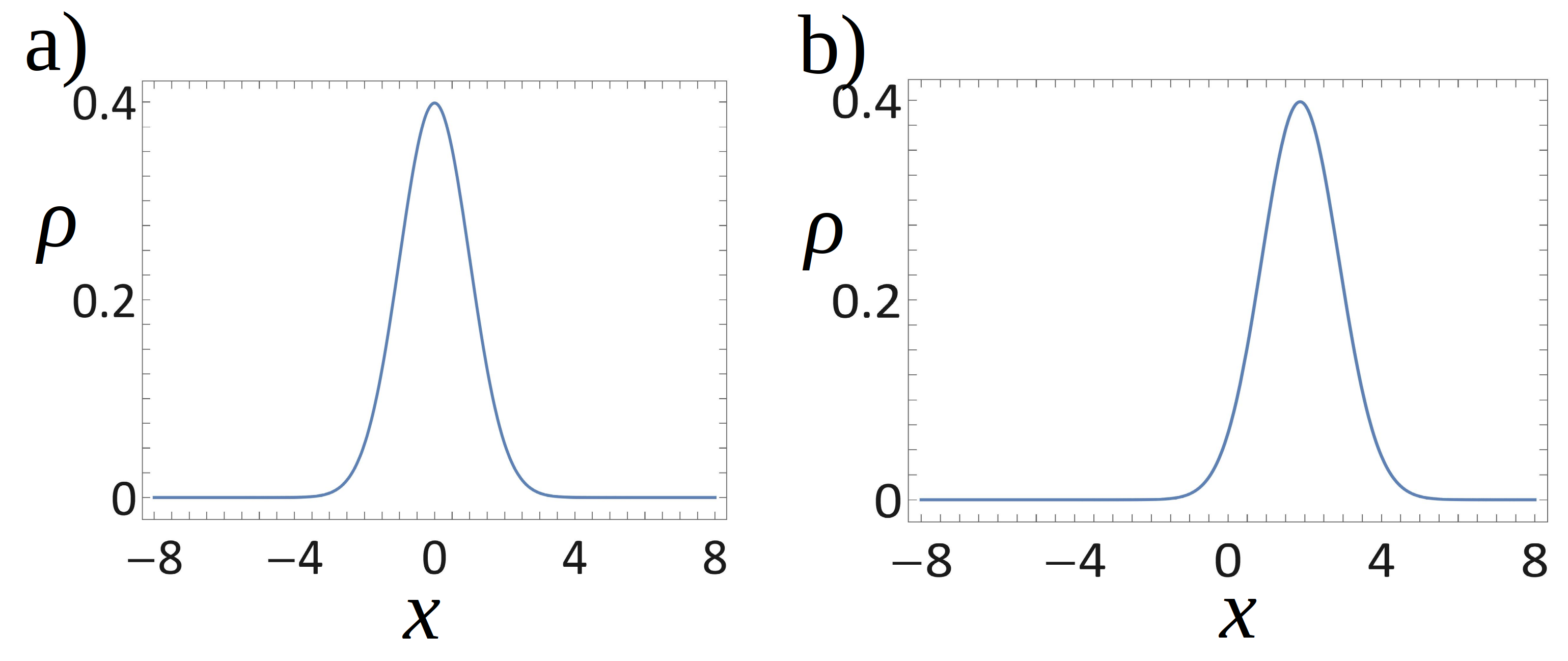
Figure 3: The uncoupled Klein-Gordon density of a spin-0 boson (a) at $t=0$ and (b) at $t=2$ (in natural units). The density at $t=0$ was chosen to be identical to the one shown in Fig. 1(a). By construction, the density (38) remains positive as the initial state evolves, as can be seen in panel (b).

IV Defining de Broglie-Bohm trajectories in the uncoupled representation

IV.1 Velocity field

We have argued above that the trouble in defining de Broglie-Bohm trajectories from the canonical KG current comes from the fact that in the canonical representation particles and anti-particles are mixed, so that the resulting charge density and current results from the quantum superposition of particle and anti-particle contributions. We propose to introduce the Bohmian velocity field from the density and current defined from the uncoupled representation. Using Eqs. (38) and (39), this gives

$$v(t,x)=\frac{J(x,t)}{\varrho(x,t)}.$$ (41)

By construction, this velocity field will not suffer from the problems due to the fluctuating sign of $\rho(x,t)$ that affect the velocity field (26) defined from the canonical KG density. As an illustration, we reconsider the example shown in Figs. 1-2. The evolution of the same Gaussian leads to a density that is everywhere positive (Fig. 3(a)-(b)). Even though this is a highly relativistic regime ($p_{0}=3mc$), the velocity field (41) is well-behaved – it takes values around the classical velocity (13) of a particle of momentum $p_{0}$ and does not lead to the appearance of superluminal velocities, as pictured in Fig. 4.

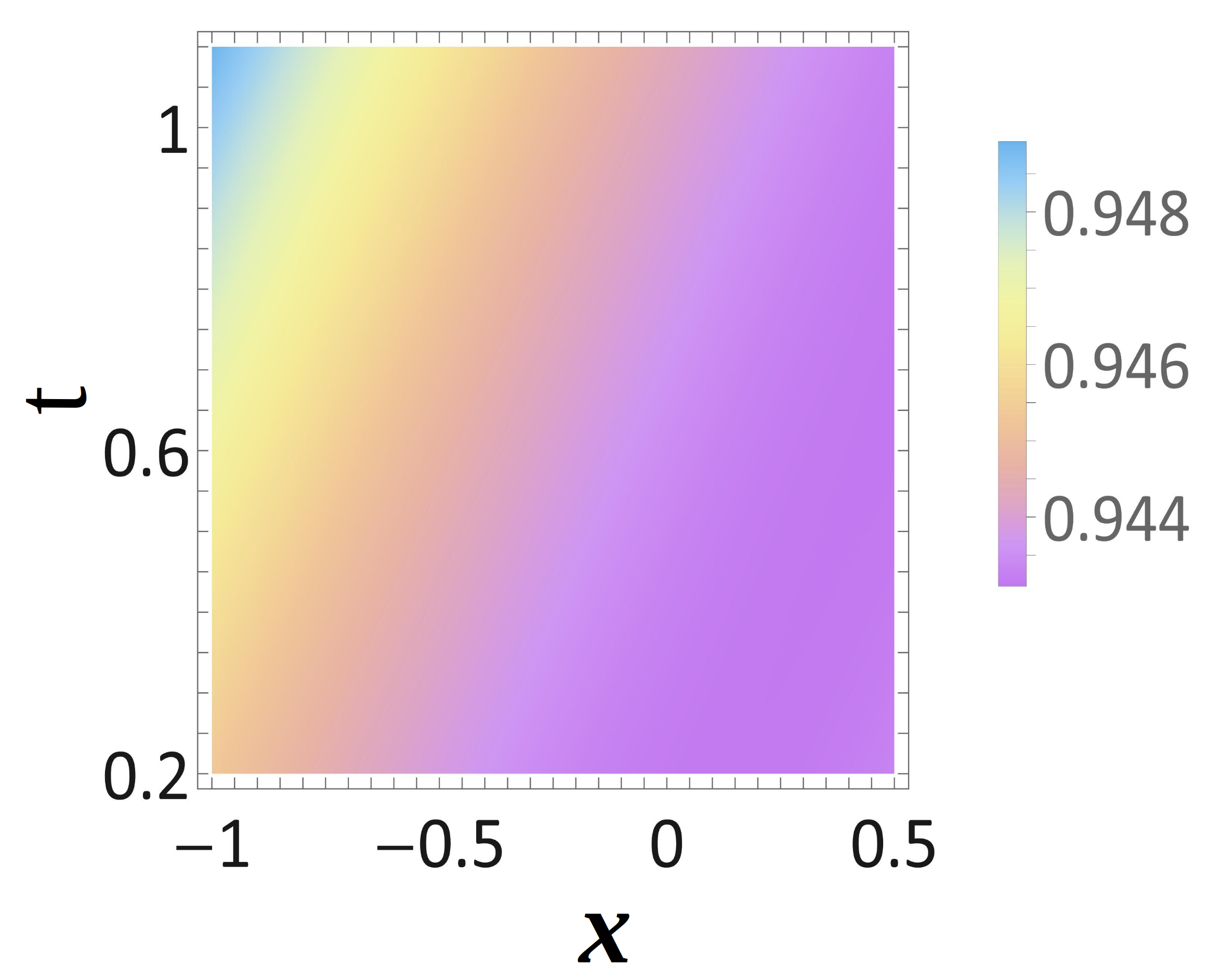
Figure 4: The velocity field defined by Eq. (41) (uncoupled Klein-Gordon velocity field) is shown (in natural units) in a given space-time region when the initial state is the one shown in Fig. 3(a). The values are all very close to the value of the classical velocity field of a particle having momentum $p_{0}$ (compare with the canonical velocity field shown in Fig. 2).

IV.2 Bohmian trajectories

Bohmian trajectories are obtained in the usual way by solving for $dx/dt=v[x(t),t)]$, with the initial condition $x(0)=x^{0}$, where $x^{0}$ lies within the initial distribution $\varrho(t=0)$. An illustration is given in Fig. 5, in which trajectories and velocities obtained from the uncoupled density and current density are shown, for an initial state identical to the one displayed in Fig. 3(a) except for the value of $p_{0}$ that is taken as $p_{0}=0.$ Note that these trajectories are similar in shape to the well-known non-relativistic de Broglie-Bohm trajectories, and show no pathological behavior, contrary to the ones defined from the canonical KG quantities.

We have not been able nevertheless to obtain strict conditions on the initial distribution ensuring that $v(x,t)$ remains subliminal, even in the case of free propagation. Numerical simulations starting from normalizable densities, including with interfering distributions and the presence of nodal structures, have all shown Bohmian trajectories with subluminal velocities, with $J(x,t)\rightarrow 0$ as $\varrho(x,t)$ vanishes.

One particular instance for which a superluminal velocity might appear concerns the exponentially small propagation of the wavefunction beyond the light cone. This is a feature obtained when a wavefunction with initial compact support is evolved with the particle (positive energy sector) propagator only. The issues with causality are usually disregarded, although the fundamental implications of this effect are poorly understood. Note that this feature is neither specific to the de Broglie Bohm formulation nor to the uncoupled representation; while the propagator in the canonical representation is fully causal, the position eigenfunctions are not delta functions but have a certain width of the order of the Compton wavelength (so that a position eigenfunction lying slightly outside the lightcone will overlap with the propagated wavefunction).

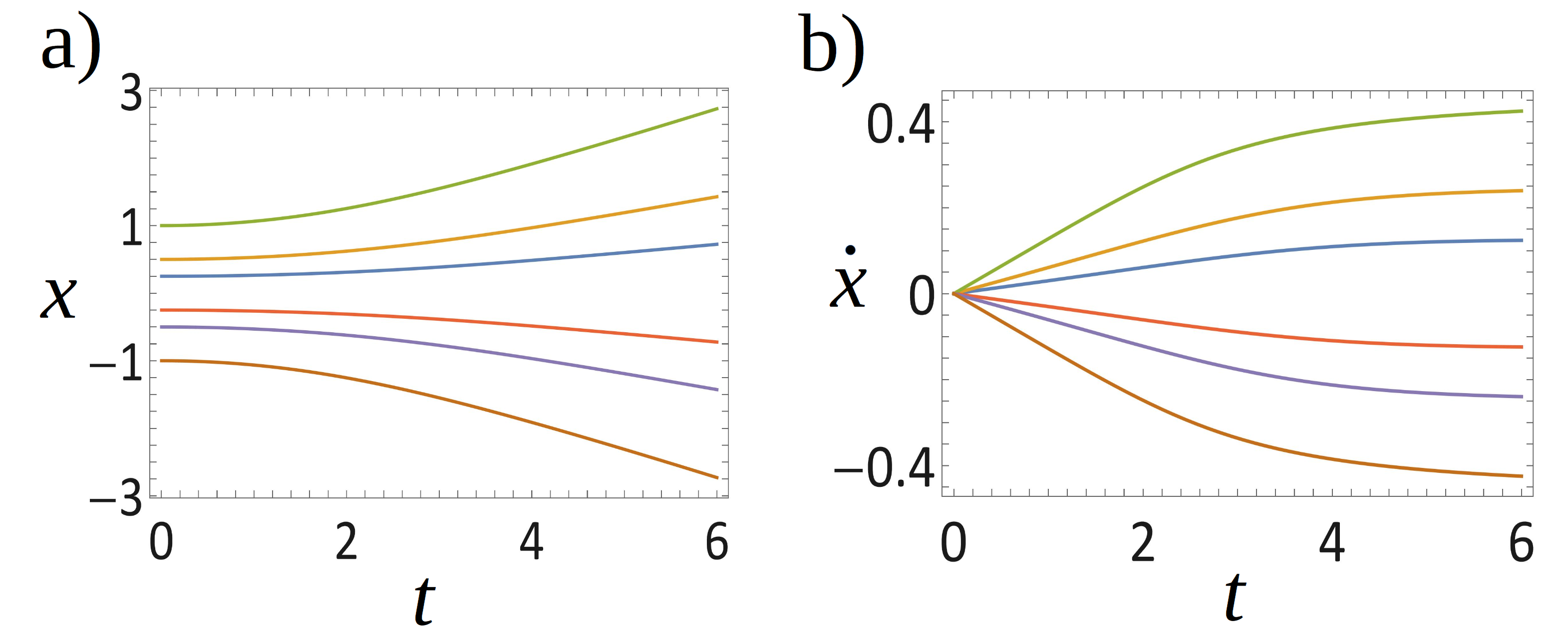
Figure 5: (a) Bohmian trajectories $x(t)$ for spin-0 bosons in the uncoupled Klein-Gordon representation. The initial state is similar to the Gaussian shown in Fig. 3(a) except for the mean momentum, taken here to be $p_{0}=0$ (the momentum distribution has therefore both positive and negative components). The initial position $x^{0}$ of each trajectory can be read off on the vertical axis. (b) Velocity $\dot{x}=dx(t)/dt$ of each Bohmian trajectory plotted in panel (a). Note that all the velocities remain sub-luminal (natural units are used, with $c=1$).

V Conclusion

We have seen in this paper how de Broglie-Bohm trajectories for massive particles obeying the Klein-Gordon equation can be obtained by working with densities and currents defined from the wavefunctions in an uncoupled representation – a representation in which the particle (positive energy) and anti-particles (negative energy) sectors are separated. This solves in principle the main specific issues affecting Bohmian trajectories obtained from the canonical representation of the KG equation, that we have attributed to the superposition of positive and negative energy contributions. It should be emphasized that the uncoupled representation is instrumental in order to understand the physical meaning of the quantum operators and to establish relations involving semi-classical expansions, the classical limit, and the non-relativistic limit as well.

However, additional work is needed in order to understand the dynamical properties of the trajectories, for different initial distributions and in the presence of potential and vector couplings. The matrix $U$ uncoupling the particle from the anti-particle components depends on the Hamiltonian and can seldom be obtained in closed form as was the case in Eq. (27). For Hamiltonians with arbitrary potentials one must then resort to iterative methods silenko ; jentsch in order to find the Foldy-Wouthuysen transformation.

Most of the issues will actually hinge on the properties of the uncoupled densities and current densities. These quantities are not well-known, and their use remains controversial (see e.g. the recent criticism FW-byal and the reply FW-reply ). The main fundamental issue is the lack of manifest covariance of the density rembl : no covariant 4-current can be constructed if Eq. (38) is taken as the 0-component of such a current hoffmann . Note that the existence of a preferred frame, hypothesized by Bell bell , necessarily appears in one form or another in relativistic Bohmian mechanics durr ; drezet . Finally it should remembered that the first quantized formalism breaks down when particle creation and annihilation cannot be neglected. At this point a proper quantum field theory treatment is needed; QFT accounts within the de Broglie-Bohm viewpoint have been proposed jpa-qft ; struyve ; niko-qft .

To sum up, we have introduced a method to define and compute Bohmian trajectories for the massive Klein-Gordon equation. As a proof of principle we have determined such trajectories for a free Hamiltonian, and checked that their properties are devoid of the serious problems that have led up to now to renounce to a trajectory interpretation for spin-0 bosons. This work hence fills a gap between the non-relativistic trajectories and the quantum field theory accounts of the de Broglie-Bohm model.

References

- (1) L. De Broglie, J. Phys. Radium, 8, .225 (1927).
- (2) D. Bohm, Phys. Rev. 85, 166 (1952) ; Phys. Rev. 85, 180 (1952).
- (3) D. Bohm and B. J. Hiley, The Undivided Universe (Routledge, London, 1993).
- (4) G. Horton, C. Dewdney, and U. Ne’eman, Found. Phys. 32, 463 (2002).
- (5) P. R.Holland, Phys. Rep. 224, 95 (1993).
- (6) T. Kyprianidis, Phys. Lett. A 111, 111 (1985).
- (7) H. Nikolic, Found. Phys. 38, 869 (2008).
- (8) N. Cufaro-Petronia, C. Dewdney, P. Holland, T. Kyprianidis and J. P. Vigier, Phys. Lett. A 106, 368 (1984).
- (9) G. Horton, C. Dewdney and A. Nesteruk, J. Phys. A: Math. Gen. 33 7337 (2000).
- (10) P. Holland, Eur. Phys. J. Plus 134, 434 (2019).
- (11) D. N. Vollick, Can. J. Phys. 99, 100 (2021).
- (12) L. L. Foldy and S. A. Wouthuysen, Phys. Rev. 78, 29 (1950).
- (13) K. M. Case, Phys. Rev. 95, 1323 (1954).
- (14) H. Feschbach and F. Villars, Rev. Mod. Phys. 30, 24 (1958).
- (15) L. Zou, P. Zhang, and A. J. Silenko, Phys. Rev. A 101, 032117 (2020).
- (16) S. E Hoffmann, J. Phys. A: Math. Theor. 52 225301 (2019).
- (17) C. R. Leavens, Found. Phys. 35, 469 (2005).
- (18) A. Matzkin, Found. Phys. 49, 298 (2019),
- (19) W. Greiner, Relativistic Quantum Mechanics (Springer, Berlin, 1996).
- (20) A. Mostafazadeh, Class. Quantum Grav. 20 155 (2003).
- (21) M. Alkhateeb, X. Gutiérrez de la Cal, M. Pons, D. Sokolovski, and A. Matzkin, Phys. Rev. A 103, 042203 (2021).
- (22) P. R. Holland, The Quantum Theory of Motion (Cambridge University Press, Cambridge, England, 1993), Sec. 12.1.
- (23) L. de Broglie, Non-linear wave mechanics (Elsevier, Amsterdam, 1960), Ch. 9, Sec. 2. [originally published as L. de Broglie, Une interprétation causale et non linéaire de la Mécanique ondulatoire: la théorie de la double solution (Gauthier-Villars, Paris, 1956)].
- (24) H. Nikolic, Found. Phys. Lett. 17, 363 (2004).
- (25) A. Matzkin and V. Nurock, Studies in Hist. and Phil. of Science B 39, 17 (2008).
- (26) A. Matzkin, Found. Phys. 39, 903 (2009).
- (27) T. D. Newton and E. P. Wigner, Rev. Mod. Phys. 21, 400 (1949).
- (28) J. P. Costella and B. H. J. McKellar, Am. J. Phys. 63 1119 (1995).
- (29) K. Kowalski and J. Rembielinski, Phys. Rev. A 84, 012108 (2011).
- (30) A. Wienczek, C. Moore and U. D. Jentschura, Phys. Rev. A 106, 012816 (2022).
- (31) I. Bialynicki-Birula and Z. Bialynicka-Birula, Phys. Rev. Lett. 122, 159301 (2019).
- (32) A. J. Silenko, P. Zhang, and L. Zou, Phys. Rev. Lett. 122, 159302 (2019).
- (33) J. Rembielinski and K. A. Smolinski, EPL 88 10005 (2009).
- (34) J. S Bell, “Quantum mechanics for cosmologists”, reprinted in J. S Bell, Speakable and unspeakable in quantum mechanics, 2nd edition (Cambridge University Press, Cambridge, England, 2004), Ch. 15.
- (35) D. Durr, S. Goldstein, T. Norsen, W. Struyve and N. Zanghi, Proc. R. Soc. A.470 20130699 (2014).
- (36) A. Drezet, Found Phys 49, 1166 (2019).
- (37) D. Durr, S. Goldstein, R. Tumulka and N. Zanghi, J. Phys. A: Math. Gen. 36 4143 (2003).
- (38) W. Struyve, Rep. Prog. Phys. 73 106001 (2010).
- (39) H. Nikolic, Int. J. Mod. Phys. A 25, 1477 (2010).