On single-photon and classical interference

Abstract

It has often been remarked that single-photon interference experiments, however complicated, seem to behave very much in the same way as those performed in the classical regime, using the field generated by a laser. This observation has the status of being ‘well-known to those who know it’, but perhaps mysterious to others. We discuss the reasons underlying the similarity and also some of the limitations of this simple idea.

I Introduction

Modern quantum optics and quantum information have encouraged the development of experiments using single photons or, to be more precise, in the single-photon regime. The most popular way of generating these is to employ spontaneous parametric downconversion, which prepares entangled photon pairs and uses one of these to herald the presence of the other Burnham ; Friberg ; MW . This heralded photon is then available for the desired experiment or application. As part of the operation a laser field is often used to assist with alignment and other practical considerations before employing the single photon source, with the measured intensity at various output ports being proportional to the anticipated detection probabilities in the single-photon regime. It is noteworthy, moreover, that a number of important experiments reporting quantum behaviour have used a laser source, sometimes attenuated, rather than single photons, in the expectation that a single photon would behave in the same manner. A few examples may be in order: quantum key distribution with weak laser pulses PaulSimon ; Norbert , optimal measurements for quantum state discrimination SarahRev , quantum walks Christine and demonstrations of the benefits of indefinite causal order Jacqui .

We seek to explain the reason why classical (laser-based) and single-photon interference experiments are so similar. Our analysis is based on the behaviour of coherent states of light, which provide the closest approximation, within quantum theory to a classical radiation field Glauber66 ; Klauder ; GlauberBook . The properties of coherent states and, in particular, the way in which fields prepared in coherent states interfere provide simple explanations for the similarity between classical and single-photon interference experiments.

It is important to realise that there are distinct differences between coherent states, even those with a very small amplitude, and genuine single photons. We conclude with a discussion of two of these differences: photon anti-bunching QTL3 ; Alain and the two-photon Hong-Ou-Mandel effect MW ; HOM .

II Classical and quantum theories of interference

To address our question we need to make precise a working definition of an interferometer. We define an interferometer as a device comprising only passive linear optical elements, principally beam splitters, mirrors and wave-plates, with input ports into which light can be directed and output ports which record either photocounts in the single photon regime or photocurrents proportional to the laser intensity. It is certainly possible to construct interferometrers that include more complicated elements, such as nonlinear media, but including these tends to invalidate the link between laser-based experiments and those utilising single photons. Examples of suitable devices include the familiar Mach-Zehnder and Michelson interferometers, but also the famous Young two-slit experiment. The components in these devices coherently superpose light from interfering modes, redirect light and rotate polarisations. They do not add photons to the field although lossy elements may remove them.

Figure 1: Schematic representation of a beam splitter. In the classical theory, input modes with complex amplitudes $a_{1}$ and $a_{2}$ are superposed to form the output amplitudes $b_{1}$ and $b_{2}$. In the quantum theory these complex amplitudes are replaced by photon annihilation operators.

A key element in many practical interferometers is the beam splitter, depicted in Figure 1. In the classical theory this combines two modes with complex amplitudes $a_{1}$ and $a_{2}$ to produce two output modes with amplitudes $b_{1}$ and $b_{2}$. For simplicity we consider a symmetric beam splitter for which the two sets of amplitudes are related by QTL3

$$b_{1}=ta_{1}+ra_{2}\qquad b_{2}=ta_{2}+ra_{1}\,.$$ (1)

The intensity is proportional to the modulus squared of these amplitudes and it follows that the total output intensity is proportional to

$$|b_{1}|^{2}+|b_{2}|^{2}=(|t|^{2}+|r|^{2})(|a_{1}|^{2}+|a_{2}|^{2})+(t^{*}r+r^{*}t)(a_{1}^{*}a_{2}+a_{2}^{*}a_{1})\,.$$ (2)

As it stands this expression depends on the relative phase between the amplitudes $a_{1}$ and $a_{2}$, but the values of $t$ and $r$, being fixed properties of the beam splitter, cannot depend on this relative phase so we can infer that $t^{*}r+r^{*}t=0$, so that $t^{*}r$ is imaginary. Conservation of energy then requires that $|t|^{2}+|r|^{2}=1$. In the quantum theory we can replace the field amplitudes by photon annihilation operators so that our classical relationship in Equation 1 is replaced by the operator form

$$\hat{b}_{1}=t\hat{a}_{1}+r\hat{a}_{2}\qquad\hat{b}_{2}=t\hat{a}_{2}+r\hat{a}_{1}\,.$$ (3)

The same relationships between $t$ and $r$ as found in the classical theory can now be derived from the commutation relations $[\hat{b}_{i},\hat{b}_{j}^{\dagger}]=\delta_{ij}=[\hat{a}_{i},\hat{a}_{j}^{\dagger}]$.

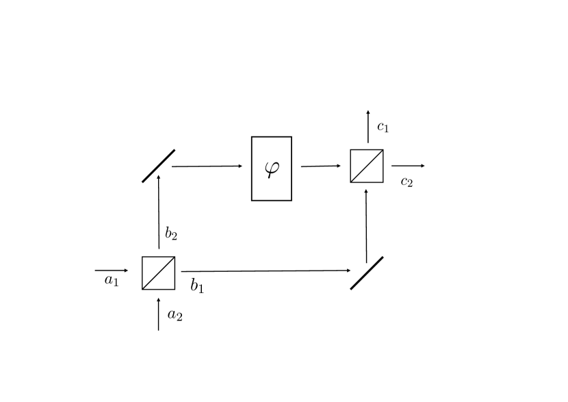
Figure 2: Schematic representation of a Mach-Zehnder interferometer. The input beam splitter is as in Figure 1 with transmission and reflection coefficients $t_{1}$ and $r_{1}$. The lengths of the two arms are $L_{1}$ and $L_{2}$ so that propagation along the arms produces the phase shifts $kL_{1}$ and $kL_{2}$. For completeness, we include, also an additional element in the upper arm producing an additional phase shift $\varphi$.

As an example we consider a simple Mach-Zehnder interferometer as depicted in Figure 2. It is straightforward to determine the forms of the output amplitudes, $c_{1}$ and $c_{2}$ or, in quantum theory, the output annihilation operators in terms of the input ones.

$$c_{1} =(t_{2}t_{1}e^{ikL_{1}}+r_{2}r_{1}e^{i\varphi}e^{ikL_{2}})a_{1}+(t_{2}r_{1}e^{ikL_{1}}+r_{2}t_{1}e^{i\varphi}e^{ikL_{2}})a_{2}$$

$$c_{2} =(t_{2}r_{1}e^{i\varphi}e^{ikL_{2}}+r_{2}t_{1}e^{ikL_{1}})a_{1}+(t_{2}t_{1}e^{i\varphi}e^{ikL_{2}}+r_{1}r_{2}e^{ikL_{1}})a_{2}\,.$$ (4)

If we input light only in mode $a_{1}$, then the intensities at the outputs will be proportional to the quantities

$$|c_{1}|^{2} =|t_{2}t_{1}e^{ikL_{1}}+r_{2}r_{1}e^{i\varphi}e^{ikL_{2}}|^{2}|a_{1}|^{2}$$

$$|c_{2}|^{2} =|t_{2}r_{1}e^{i\varphi}e^{ikL_{2}}+r_{2}t_{1}e^{ikL_{1}}|^{2}|a_{1}|^{2}\,.$$ (5)

We can think of the quantity $|t_{2}t_{1}e^{ikL_{1}}+r_{2}r_{1}e^{i\varphi}e^{ikL_{2}}|^{2}$ as the probability that any one photon in the input emerges in mode $c_{1}$ and $|t_{2}r_{1}e^{i\varphi}e^{ikL_{2}}+r_{2}t_{1}e^{ikL_{1}}|^{2}$ as the probability that it emerges in mode $c_{2}$. We can check this interpretation by turning to the quantum description, where we find that the annihilation operators for the output modes are related to those of the input by

$$\hat{c}_{1} =(t_{2}t_{1}e^{ikL_{1}}+r_{2}r_{1}e^{i\varphi}e^{ikL_{2}})\hat{a}_{1}+(t_{2}r_{1}e^{ikL_{1}}+r_{2}t_{1}e^{i\varphi}e^{ikL_{2}})\hat{a}_{2}$$

$$\hat{c}_{2} =(t_{2}r_{1}e^{i\varphi}e^{ikL_{2}}+r_{2}t_{1}e^{ikL_{1}})\hat{a}_{1}+(t_{2}t_{1}e^{i\varphi}e^{ikL_{2}}+r_{1}r_{2}e^{ikL_{1}})\hat{a}_{2}\,.$$ (6)

If we have just a single photon prepared in mode $a_{1}$ and none in mode $a_{2}$ then $\langle\hat{a}_{1}^{\dagger}\hat{a}_{1}\rangle=1$ and $\langle\hat{a}_{2}^{\dagger}\hat{a}_{2}\rangle=0$. It follows that the probabilities that the photon leaves the interferometer in mode $c_{1}$ or $c_{2}$ are

$$\langle\hat{c}_{1}^{\dagger}\hat{c}_{1}\rangle =|t_{2}t_{1}e^{ikL_{1}}+r_{2}r_{1}e^{i\varphi}e^{ikL_{2}}|^{2}$$

$$\langle\hat{c}_{2}^{\dagger}\hat{c}_{2}\rangle =|t_{2}r_{1}e^{i\varphi}e^{ikL_{2}}+r_{2}t_{1}e^{ikL_{2}}|^{2}$$ (7)

respectively. These are precisely the quantities inferred from the classical description.

In the following section we shall address the question of why the single-photon probabilities arise so simply in the classical theory and, in doing so, establish that the equivalence is general and may be applied to any interferometric device. Before turning to this, it is instructive to recall what three others (among many) have written on this point. We start with the famous quote from Dirac Dirac :

Suppose we have a beam of light consisting of a large number of photons split up into two components of equal intensity. On the assumption that the intensity of a beam is connected with the probable number of photons in it, we should have half the total number of photons going into each component. If the two components are now made to interfere, we should require a photon in one component to be able to interfere with one in the other. Sometimes these two photons would have to annihilate one another and other times they would have to produce four photons. This would contradict the conservation of energy. The new theory, which connects the wave function with probabilities for one photon, gets over the difficulty by making each photon go partly into each of the two components. Each photon then interferes only with itself. Interference between two different photons never occurs.

In the first edition of his book, The Quantum Theory of Light, Loudon writes of Young’s interference experiment QTL1 :

Photons do not interact with each other, and any interference effects must be sought in the process by which each single photon passes from the source to the second screen. Quantum-mechanically, the interference occurs between the probability amplitudes for passage from source to screen via the two different paths corresponding to the two pinholes. The intensity on the second screen is proportional to the square modulus of the sum of the two probability amplitudes. The structure of the quantum-mechanical calculation is the same as that of the classical calculation, which is also based of the sum of two amplitudes, and the two calculations give the same intensity distribution.

Finally, in Jex’s translation of Paul’s book, Introduction to Quantum Optics, we find Paul :

Let us note that the quantized theory of the electromagnetic field encompasses the particle equally well as the wave aspect. In particular, beamsplitting can be described in such a way that (in complete correspondence to classical theory) the electric field strength - now described by an operator - of the incident wave is decomposed into parts corresponding to the reflected wave and the transmitted wave. We find then the surprising (at least at first glance) result that the classical interference pattern is quantum mechanically exactly reproducible independent of the (perhaps even non-classical) state of the incident light.

The common point emphasised by each of these accounts is that in interference, as we have discussed it, single photons within a beam of light behave, individually, in the same manner as would a field in the classical theory.

III Interfering coherent states

The key to deriving our desired result, that single-photon interference experiments behave precisely as do classical ones, lies in the properties of the coherent states. For any single mode, with annihilation and creation operators, $\hat{a}$ and $\hat{a}^{\dagger}$, the coherent state is a displaced vacuum obtained by means of a unitary transformation MW ; Glauber66 ; Klauder ; GlauberBook ; QTL3 ; Methods :

$$|\alpha\rangle=\hat{D}(\alpha)|0\rangle=\exp\left(\alpha\hat{a}^{\dagger}-\alpha^{*}\hat{a}\right)|0\rangle\,.$$ (8)

Two properties of the coherent states will be useful to us. The first of these is that the coherent states are right-eigenstates of the annihilation operator with eigenvalue $\alpha$:

$$\hat{a}|\alpha\rangle=\alpha|\alpha\rangle\,.$$ (9)

The second is that the coherent state is a superposition of photon number states in the form

$$|\alpha\rangle=e^{-|\alpha|^{2}/2}\sum_{n=0}^{\infty}\frac{\alpha^{n}}{\sqrt{n!}}|n\rangle\,.$$ (10)

From the eigenvalue property we can determine how coherent state combine when superposed on a beam splitter. In Equation (3) we have, essentially, a Heisenberg picture relation between the output and input modes for a simple beam splitter. If we prepare each input mode in a coherent state, $|\alpha_{1}\rangle$ and $|\alpha_{2}\rangle$ respectively, then it follows that the state is a right-eigenstate of the output annihilation operators $\hat{b}_{1}$ and $\hat{b}_{2}$:

$$\hat{b}_{1}|\alpha_{1}\rangle|\alpha_{2}\rangle =(t\alpha_{1}+r\alpha_{2})|\alpha_{1}\rangle|\alpha_{2}\rangle$$

$$\hat{b}_{2}|\alpha_{1}\rangle|\alpha_{2}\rangle =(t\alpha_{2}+r\alpha_{1})|\alpha_{1}\rangle|\alpha_{2}\rangle\,.$$ (11)

It follows that, in the Schrödinger picture, the states of the output modes are also coherent states, $|\beta_{1}\rangle$ and $|\beta_{2}\rangle$ respectively, where $\beta_{1}=t\alpha_{1}+r\beta_{2}$ and $\beta_{2}=t\alpha_{2}+r\beta_{1}$. Hence the complex amplitudes of our coherent states combine in precisely the same manner as do the classical amplitudes. This conclusion applies to each of our passive linear optical elements and, indeed, to any interferometer, however complicated. This property was first obtained in the context of coupled oscillators by Glauber GlauberPL . It may be of interest to note that this idea can readily be extended to any state of light by writing such states as a superposition of coherent states JanszkySMB .

Another way to see the relationship between the coherent state amplitudes and the amplitudes in the classical theory is to adopt the vacuum picture Mollow ; Samson ; David ; PMRPLK . To see how this works consider a single mode of the field in which the electric field operator has the form

$$\hat{\bf E}={\bf E}_{0}u({\bf r})e^{-i\omega t}\hat{a}+{\bf E}^{*}_{0}u^{*}({\bf r})e^{i\omega t}\hat{a}^{\dagger}\,,$$ (12)

where $u({\bf r})$ is the spatial mode function. Let this mode be prepared in the coherent state $|\alpha\rangle$. We can transform into the vacuum picture by acting on the state with the unitary operator $\hat{D}^{\dagger}(\alpha)=\hat{D}(-\alpha)$, which leaves the field mode in its vacuum state, $|0\rangle$. To keep the physical situation unchanged we need, also, to transform the operators $\hat{O}\rightarrow\hat{D}^{\dagger}(\alpha)\hat{O}\hat{D}(\alpha)$. For our electric field operator, this transformation produces the operator

$$\hat{D}^{\dagger}(\alpha)\hat{\bf E}\hat{D}(\alpha)=\hat{\bf E}+{\bf E}_{0}u({\bf r})e^{-i\omega t}\alpha+{\bf E}^{*}_{0}u^{*}({\bf r})e^{i\omega t}\alpha^{*}\,,$$ (13)

which is a superposition of the electric field operator and a classical field with an amplitude proportional to $\alpha$. The passive optical elements leave the vacuum field unchanged; zero photons in leads to zero photons out, and the c-number amplitudes behave as do the amplitudes in the classical theory. It follows that a coherent state input into our interferometer behaves in precisely the same manner as the field amplitude in the classical theory.

The final step is to note that in the number-state expansion of the coherent state, the single-photon probability amplitude is proportional to $\alpha$, with the amplitude for higher photon numbers varying as $\alpha^{n}$. It follows that the single-photon probability amplitude evolves on passage through an interferometer in the same manner as the amplitude $\alpha$ and, therefore, as does the field in the classical description. This completes our proof that in an interferometer with single photon input, the probability amplitude associated with any given path through the device behaves precisely as does the amplitude of a classical field.

The simplest way to state the equivalence is that the coherent amplitude for a coherent state, $\alpha$, behaves in the same way as does a classical field amplitude. For a single photon, $\alpha$ is also the probability amplitude and the detection probability is proportional to $|\alpha|^{2}$, as is the intensity in a classical treatment.

IV Limitations

It is important not to push the above idea too far. What we have established is an equivalence between the probabilities for single detection events at the outputs of a single-photon device with the corresponding intensity measured in the same interferometer with a laser input. We consider two quantum interference phenomena that are not obtainable classically. These are photon antibunching and two-photon interference in the Hong-Ou-Mandel effect, both of which reveal themselves in the correlations between pairs of detectors.

IV.1 Photon antibunching

If we have just a single photon, then it cannot be detected in two separate detectors. This means that if we place a detector in each of the outputs from our beam splitter in Figure 1 and send a single photon in one of the input arms then we can only get a detection event in one of the two detectors. The transmission and reflection coefficients tell us the probability that the photons is transmitted or reflected and then is detected in the corresponding detector. This feature, as we have seen, is reproduced in the classical theory.

In the classical theory if $\alpha$ is the input field amplitude then the probability that a detection event occurs in both detectors is proportional to $|t|^{2}|r|^{2}|\alpha|^{4}$. More precisely, the probability of detecting light in both output detectors is always at least as big as the product of the probabilities for detections at the individual detectors, and the anticorrelation between detection events found for a single photon input cannot be reproduced in the classical theory.

The anticorrelation is crucial to the demonstration of single-photon interference. Note that the first attempt to produce single-photon interference was probably that by Taylor in 1909, who employed a heavily attenuated light source and very long exposure times (up to three months) in an attempt to determine, through the loss of visibility, the size of light quanta Taylor . We now know, as shown above, that this experiment could only produce interference fringes however faint the input light. To demonstrate true single-photon interference one needs a truly single-photon source and a means of verifying this property. This was achieved nearly eighty years after Taylor’s work Alain ; GilbertBook . A cascade emission provided a herald that a second photon was about to be emitted and this entered either an interferometer or a beam splitter followed by two detectors. The observation of high visibility fringes in the interferometer but near perfect anticorrelation in the two detectors following the beam splitter finally confirmed the quantum prediction, noted by Dirac, that each photon interferes only with itself.

IV.2 Two-photon interference

In a now classic experiment, Hong, Ou and Mandel showed that if a pair of indistinguishable photons are incident on a beam splitter, with one photon in each arm, then the output modes tend to produce an anticorrelation, with detections in both detectors suppressed. It is straightforward to confirm this using the relationships. In Equation (3), between the input and output modes:

$$\hat{a}_{1}^{\dagger}\hat{a}_{2}^{\dagger}|0\rangle =(t\hat{b}_{1}^{\dagger}+r\hat{b}_{2}^{\dagger})(r\hat{b}_{1}^{\dagger}+t\hat{b}_{2}^{\dagger})|0\rangle$$

$$=\left[tr(\hat{b}_{1}^{\dagger 2}+\hat{b}_{2}^{\dagger 2})+(t^{2}+r^{2})\hat{b}_{1}^{\dagger}\hat{b}_{2}^{\dagger}\right]|0\rangle\,.$$ (14)

Finding a photon in each output mode is suppressed owing to the phase relationship between $t$ and $r$ footnote , but the probability for finding two photons both in each of the output modes are equal. If the beam splitter is balanced so that $|t|^{2}=\frac{1}{2}=|r|^{2}$, then the coefficient of the two photon state $\hat{b}_{1}^{\dagger}\hat{b}_{2}^{\dagger}|0\rangle$ is zero and the two photons are never found in different detectors MW ; HOM .

This feature, which like antibunching depends on correlated detections or their absence, cannot be reproduced in the classical theory or, what comes to the same thing, with coherent states. To see this it suffices to consider the two-photon component of input coherent states. Let the two input modes be prepared in the coherent states $|\alpha_{1}\rangle$ and $|\alpha_{2}\rangle$. It follows that the two-photon component of the state is

$$|\psi\rangle =\frac{\alpha_{1}^{2}}{\sqrt{2}}|2\rangle_{1}|0\rangle_{2}+\alpha_{1}\alpha_{2}|1\rangle_{1}|1\rangle_{2}+\frac{\alpha_{2}^{2}}{\sqrt{2}}|0\rangle_{1}|2\rangle_{2}$$

$$=\left(\frac{\alpha_{1}^{2}}{2}\hat{a}_{1}^{\dagger 2}+\alpha_{1}\alpha_{2}\hat{a}_{1}^{\dagger}\hat{a}_{2}^{\dagger}+\frac{\alpha_{2}^{2}}{2}\hat{a}_{2}^{\dagger 2}\right)|0\rangle_{1}|0\rangle_{2}\,.$$ (15)

The corresponding (unnormalised) state of the output modes is

$$|\psi\rangle=\frac{1}{2}\left[(\alpha_{1}t+\alpha_{2}r)\hat{b}_{1}^{\dagger}+(\alpha_{1}r+\alpha_{2}t)\hat{b}_{2}^{\dagger}\right]^{2}|0\rangle_{1}|0\rangle_{2}\,.$$ (16)

The only way to remove the correlations between the two detectors, that is to set the coefficient of $\hat{b}_{1}^{\dagger}\hat{b}_{2}^{\dagger}|0\rangle_{1}|0\rangle_{2}$ equal to zero, is to set either $\alpha_{1}t+\alpha_{2}r$ or $\alpha_{1}r+\alpha_{2}t$ to be zero. In this case there is perfect interference between the coherent state amplitudes and all of the light goes into a just one of the two output modes. This is in sharp contrast to the behaviour of two single photons, noted above, in which correlations between the two detectors are suppressed, but the two photons are equally likely to be found in either output mode.

V Conclusion

It has long been recognised that single-photon interference experiments behave, essentially, in the same way as those performed with far more intense fields such as those generated by a laser. At the heart of this is the familiar statement by Dirac that “each photon then interferes only with itself” Dirac . Our aim in writing this paper is to explore precisely why this is so. We have found that, as is often the case in quantum optics, the coherent states provide a natural way of linking single photon (quantum) behaviour with that of laser-light (classical) behaviour. The key idea is that the complex amplitude, $\alpha$, associated with a coherent state behaves in precisely the same manner as does the classical, c-number, amplitude in the quantum theory of interference. Moreover, this same amplitude is that of the single photon component of the coherent state.

It is important to appreciate that there are limitations to the association between single-photon and classical interference. In particular we are limited to devices constructed from passive linear optical elements as these conserve the photon number. The forms of measurement are also restricted; we can compare single-photon detection events only, that is the probabilities for detecting the single photon at any given detector, and compare these with the fraction of the intensity recorded in the same output port in the classical treatment. It is by observing the correlations between pairs of detectors (or more) that quantum effects become apparent. We presented two classic examples of this: anticorrelation at a pair of detectors in the single photon regime and two-photon interference in the classical Hong-Ou-Mandel experiment.

We have concentrated exclusively on passive linear optical elements and by doing so have found a very general equivalence between the behaviour of single-photon and classical behaviours. This does not mean, however, that such an equivalence will never hold in devices that include nonlinear optical elements. One important example is a recent realisation of quantum teleportation in which the state to be teleported is encoded first on a laser field and is then teleported to a distant single photon Bereneice . One nonlinear optical process produces a pair of entangled photons as is often the starting point in a teleportation experiment QI . The comparison step is achieved by a frequency conversion arrangement in which one of the entangled photons (the local photon) interacts with the laser field to produce a new photon carrying information from both the previously entangled photon and the laser field. The teleportation may be viewed as the transfer of the state of one of the laser photons to the distant and previously entangled photon. As with single photon interference, this laser-based teleportation does not share all of the features of a single-photon teleportation; it cannot teleport entanglement for example. It does, nevertheless, transfer the state of the laser photons to the distant photon and it does this without using knowledge of the state of the laser photons and this, of course, is the key feature of quantum teleportation.

References

References

- (1) Burnham D C and Weinberg D L 1970 Observation os simultaneity in parametric production of optical photon pairs Phys. Rev. Lett. 25 84–87
- (2) Friberg S, Hong C K and Mandel L 1985 Measurement of time delays in the parametric production of photon pairs Phys. Rev. Lett. 54 2011–2013
- (3) Mandel L and Wolf E 1995 Optical Coherence and Quantum Optics (Cambridge: Cambridge University Press)
- (4) Phoenix S J D and Townsend P D 1995 Quantum cryptography: how to beat the code breakers using quantum mechanics Contemp. Phys. 36 165–195
- (5) Scarani V, Bechmann-Pasquinucci H, Cerf N J, Dušek M, Lütkenhaus N and Peev M 2009 The security of practical quantum key distribution Rev. Mod. Phys. 81 1301–1350
- (6) Barnett S M and Croke S 2008 Quantum state discrimination Adv. Opt. Photon. 1 238–278
- (7) Schreiber A, Cassemiro K N, Potoček V, Gábris A, Mosley P J, Andersson E, Jex I and Silberhorn C 2010 Photons walking the line: a quantum walk with adjustable coin operations Phys. Rev. Lett. 104 050502
- (8) Goswami K and Romero J 2020 Experiments on quantum causality AVS Quantum Sci 2 037101
- (9) Glauber R J 1966 Coherent and incoherent states of the radiation field Phys. Rev. 131 2766–2788
- (10) Klauder J R and Sudarshan E C G 1968 Fundamentals of Quantum Optics (New York: W A Benjamin Inc)
- (11) Glauber R J 2007 Quantum Theory of Optical Coherence (Weinheim: Wiley-VCH)
- (12) Loudon R 2000 The Quantum Theory of Light 3rd ed. (Oxford: Oxford University Press)
- (13) Grangier P, Roger G and Aspect A 1986 Experimental evidence for a photon anticorrelation effect on a beam splitter: a new light on single-photon interferences Europhys. Lett. 1 173–179
- (14) Hong C K, Ou Z Y and Mandel L 1987 Measurement of subpicosecond time intervals between two photons by interference Phys. Rev. Lett. 59 2044–2046
- (15) Dirac P A M 1958 The Principles of Quantum Mechanics 4th ed. (Oxford: Oxford University Press)
- (16) Loudon R 1973 The Quantum Theory of Light 1st ed. (Oxford: Oxford University Press)
- (17) Paul H 2004 Introduction to Quantum Optics (Cambridge: Cambridge University Press)
- (18) Barnett S M and Radmore P M 1997 Methods in Theoretical Quantum Optics (Oxford: Oxford University Press)
- (19) Glauber R J 1966 Classical behavior of systems of quantum oscillators Phys. Lett. 21 650–652
- (20) Barnett S M 2018 Schrödinger picture analysis of the beam splitter: an application of the Janszky representation J. Russ. Laser Res. 39 340–348
- (21) Mollow B R 1975 Pure-state analysis of resonant light scattering: radiative damping, saturation, and multiphoton effects Phys. Rev. A 12 1919–1943
- (22) Samson R and Ben-Reuven A 1975 The external field approximation in quantum optics Chem. Phys. Lett. 36 523–526
- (23) Pegg D T 1980 Atomic spectroscopy: interaction of atoms with coherent fields, in Laser Physics Walls D F and Harvey J D eds. (Sydney: Academic Press)
- (24) Knight P L and Radmore P M 1982 Quantum origin of dephasing and revivals in the coherent-state Jaynes-Cummings model Phys. Rev. A 26 676–679
- (25) Taylor G I 1909 Interference fringes with feeble light Proc. Cam. Phil. Soc. 15 114–115: Reprinted in Knight P L and Allen L 1983 Concepts of Quantum Optics (Oxford: Pergamon Press)
- (26) Grynberg G, Aspect A and Fabre C 2010 Introduction to Quantum Optics (Cambridge: Cambridge University Press)
-
(27)
This follows on writing
- (28) Sephton B, Vallés A, Nape I, Cox M A, Steinlechner F, Konrad T, Torres J P, Roux F S and Forbes A 2022 High-dimensional spatial teleportation enabled by nonlinear optics arXiv:2111.13624
- (29) Barnett S M 2009 Quantum Information (Oxford: Oxford University Press)