Towards Communication-efficient Vertical Federated Learning Training via Cache-enabled Local Updates

Abstract.

Vertical federated learning (VFL) is an emerging paradigm that allows different parties (e.g., organizations or enterprises) to collaboratively build machine learning models with privacy protection. In the training phase, VFL only exchanges the intermediate statistics, i.e., forward activations and backward derivatives, across parties to compute model gradients. Nevertheless, due to its geo-distributed nature, VFL training usually suffers from the low WAN bandwidth.

In this paper, we introduce CELU-VFL, a novel and efficient VFL training framework that exploits the local update technique to reduce the cross-party communication rounds. CELU-VFL caches the stale statistics and reuses them to estimate model gradients without exchanging the ad hoc statistics. Significant techniques are proposed to improve the convergence performance. First, to handle the stochastic variance problem, we propose a uniform sampling strategy to fairly choose the stale statistics for local updates. Second, to harness the errors brought by the staleness, we devise an instance weighting mechanism that measures the reliability of the estimated gradients. Theoretical analysis proves that CELU-VFL achieves a similar sub-linear convergence rate as vanilla VFL training but requires much fewer communication rounds. Empirical results on both public and real-world workloads validate that CELU-VFL can be up to six times faster than the existing works.

PVLDB Reference Format:
PVLDB, 15(10): 2111 - 2120, 2022.
doi:10.14778/3547305.3547316

PVLDB Artifact Availability:
The source code, data, and/or other artifacts have been made available at %leave␣empty␣if␣no␣availability␣url␣should␣be␣set%\newcommand\vldbavailabilityurl{}https://github.com/ccchengff/FDL/tree/main/playground/celu_vfl.

1. Introduction

The past few years have witnessed the explosion of federated learning (FL) research and applications  (Yang et al., 2019a; Li et al., 2020a; Konečný et al., 2016a, b), where two or more parties (participants) collaboratively train a machine learning (ML) model using their own private data. In particular, vertical FL (VFL) illustrates such a scenario where different parties hold disjoint features but overlap on a set of instances. As shown in Figure 1, the overlapping instances are regarded as a virtual dataset that is vertically partitioned. There are two types of parties: (i) one or more Party $\mathcal{A}$’s that merely provide features; and (ii) one Party $\mathcal{B}$ that holds both features and the ground truth labels for the learning tasks. The goal of VFL is to fit the labels by the features of all parties, whilst keeping the private data (including both features and labels) of each party secret from the others. VFL is suitable for a variety of cross-enterprise collaborations. For instance, Party $\mathcal{A}$ can be an Internet company that is able to generate rich and precise user profiling, whilst Party $\mathcal{B}$ can be an e-commercial company that hopes to build a better recommender system. As a result, VFL is gaining more popularity in both academia and industry  (Fu et al., 2021; Yang et al., 2019b; Cheng et al., 2021; Wu et al., 2020).

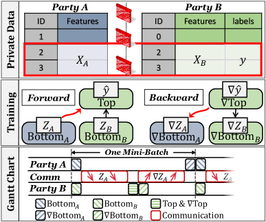
Figure 1. An illustration of VFL. The cross-party communication (indicated by red arrows) dominates the time cost of training.

(Communication Bottleneck of VFL) Denote $y$ as the labels owned by Party $\mathcal{B}$, and $X_{A},X_{B}$ as the features of Party $\mathcal{A}$ and Party $\mathcal{B}$, respectively, where the $k$-th rows $X_{A,k},X_{B,k}$ together form the features of the $k$-th instances. As shown in Figure 1, VFL models typically follow a bottom-to-top architecture. First, each Party $\mathcal{P}$ is associated with a bottom model that works as a feature extractor. It takes $X_{P}$ as input and outputs $Z_{P}=\texttt{Bottom}_{P}(X_{P};\theta_{Bot\_P})$, where $\theta_{Bot\_P}$ are the bottom model weights. Second, Party $\mathcal{B}$ is further associated with a top model parameterized by $\theta_{Top}$ that makes predictions via $\hat{y}=\texttt{Top}(Z_{A},Z_{B};\theta_{Top})$. The goal of VFL training is to find the model weights minimizing the empirical risk:

(1) $$\small\operatorname*{arg\,min}_{\left\{\theta_{Bot\_A},\theta_{Bot\_B},\theta_{Top}\right\}}\;L\coloneqq\sum_{k}l(y_{k},\hat{y}_{k}),$$

where $l$ is the loss function (e.g., the logistic loss).

The most common avenue to solve such a supervised ML problem is to adopt the mini-batch stochastic gradient descent (SGD) algorithm or its variants. For each step, a batch of instances is sampled to compute the model gradients $\nabla\theta=\partial L/\partial\theta$ for model updates. However, since Party $\mathcal{A}$ must not get access to the labels or the top model due to the privacy consideration, it cannot accomplish the backward propagation process alone. To overcome this problem, existing VFL frameworks adopt a two-phase propagation routine — the gradients for $\theta_{Bot\_A}$ are calculated via $\nabla\theta_{Bot\_A}=\nabla Z_{A}\frac{\partial Z_{A}}{\partial\theta_{Bot\_A}}$, where $\nabla Z_{A}=\partial L/\partial Z_{A}$ are provided by Party $\mathcal{B}$.

As shown in the Gantt chart of Figure 1, in each step, two kinds of intermediate data are transmitted, i.e., forward activations $Z_{A}$ and backward derivatives $\nabla Z_{A}$. In practice, the communication cost is expensive due to the limited network bandwidth. Since the data centers of different parties are usually physically distributed, VFL tasks have to run in a geo-distributed manner where Wide Area Network (WAN) bandwidth is very low. For instance, as reported by Qian et al. (2021) and verified by our empirical benchmark, the bandwidth between different data centers are usually smaller than 300 Mbps. Worse still, since most companies have network restrictions to avoid external attacks, the servers that carry out the VFL tasks are forbidden from connecting to WAN directly. Instead, messages are proxied by some gateway machines, leading to even slower communication. Eventually, in real-world VFL applications, we observe that over 90% of the total training time is spent on communication, leading to extremely low efficiency and a huge waste of computational resources. Consequently, how to tackle the communication bottleneck in VFL is a timely and important problem.

1

2foreach mini-batch $i$ do

3       Compute and send $Z_{A}^{(i)}$; Recv $\nabla Z_{A}^{(i)}$;

4       Update with $\nabla\theta_{Bot\_A}=\nabla Z_{A}^{(i)}\frac{\partial Z_{A}^{(i)}}{\partial\theta_{Bot\_A}}$;

5       for $j\leftarrow 1\textup{ until }R$ do // local updates

6             Compute $Z_{A}^{(i,j)}$; Update with $\widetilde{\nabla}\theta_{Bot\_A}=\nabla Z_{A}^{(i)}\frac{\partial Z_{A}^{(i,j)}}{\partial\theta_{Bot\_A}}$;

7            

Algorithm 1 VFL training with local updates (FedBCD (Liu et al., 2019)) for Party $\mathcal{A}$. Line 4-5 can be executed in background to overlap the communication and local updates.

(Motivation) To address the communication bottleneck, an intuitive idea is to amortize the network cost by performing multiple local updates between two communication rounds. In fact, such a local update technique (a.k.a. local SGD) has been widely studied in conventional (non-federated) distributed ML and horizontal FL  (Haddadpour et al., 2019; Stich, 2019; Konečný et al., 2016a, b). However, applying this technique in VFL is non-trivial since each party cannot accomplish the forward or backward propagation individually due to the lack of $Z_{A}$ or $\nabla Z_{A}$. Thus, approximating $Z_{A}$ or $\nabla Z_{A}$ with stale statistics is needed. Specifically, FedBCD (Liu et al., 2019) proposes to execute $R$ updates for each mini-batch, which is shown in Algorithm 1. During the $j$-th update of the $i$-th mini-batch, instead of exchanging the ad hoc values, i.e., $\langle Z_{A}^{(i,j)},\nabla Z_{A}^{(i,j)}\rangle$, Party $\mathcal{A}$ treats $\nabla Z_{A}^{(i)}$ as an approximation and estimates the model gradients as $\widetilde{\nabla}\theta_{Bot\_A}=\nabla Z_{A}^{(i)}\frac{\partial Z_{A}^{(i,j)}}{\partial\theta_{Bot\_A}}$; symmetrically, Party $\mathcal{B}$ feeds the stale values $Z_{A}^{(i)}$ and the ad hoc values $Z_{B}^{(i,j)}$ to the top model.

Nevertheless, there are two drawbacks of local updates in VFL: (1. variance problem) using the same stale mini-batch for multiple consecutive steps would enlarge the stochastic variance in model gradients (similar phenomenon can be observed in SGD algorithms without data shuffling (Mishchenko et al., 2020; Feng et al., 2012; Xu et al., 2022)); (2. approximation errors) because approximation via stale statistics inevitably introduces errors to the model gradients, it would slow down the convergence or even lead to divergence if we directly update the models with the approximated gradients. According to the above analysis, there exists a discrepancy in the state of VFL with local updates — doing more local steps brings a better improvement on the system efficiency, but can easily harm the statistical efficiency.

(Summary of Contributions) Motivated by this, our work proposes a novel VFL training framework that improves both system efficiency and statistical efficiency at the same time. To summarize:

• We develop CELU-VFL, an efficient VFL training framework that exploits a cache-enabled local update technique for better system efficiency. To reduce the communication cost, CELU-VFL introduces an abstraction of workset table that caches the forward activations and backward derivatives to enable the local update technique. CELU-VFL further overlaps the reads and writes of the workset table triggered by local computation and cross-party communication to improve resource utilization.

• To improve the statistical efficiency, CELU-VFL addresses the two drawbacks of local updates in VFL based on the workset table abstraction. (1) First, to tackle the variance problem, we introduce a uniform local sampling strategy — instead of repetitively using the same mini-batch, the cached statistics are fairly sampled from the workset table to execute the local updates. (2) Second, to mitigate the impact of approximation errors, we design a staleness-aware instance weighting mechanism. The essential idea is to measure the staleness using cosine similarities and control the contribution of each instance according to its staleness.

• Furthermore, we theoretically analyze the convergence property of CELU-VFL, which shows that our work achieves a similar sub-linear convergence rate as vanilla VFL training but requires much fewer communication rounds. The analysis also interprets why our uniform local sampling strategy and instance weighting mechanism improve the statistical efficiency.

• We empirically evaluate the performance of CELU-VFL through extensive experiments. First, we investigate the statistical efficiency of CELU-VFL along three dimensions, i.e., the number of local updates, the strategy of local sampling, and the weighting mechanism of staleness. Second, end-to-end evaluation on both public datasets and real-world workloads demonstrates that CELU-VFL is able to outperform the existing works by 2.65-6.27$\times$.

2. Preliminaries

2.1. Vertical Federated Learning

Owing to the establishment of lawful regulation on privacy protection (Voigt and Von dem Bussche, 2017; ccp, 2018; cdp, 2021), how to train ML models with privacy preservation is becoming a hot topic. Notably, VFL has become a prevailing paradigm that unites the features from different parties for collaborative applications  (Yang et al., 2019b; Fu et al., 2022, 2021; Cheng et al., 2021; Wu et al., 2020; Hu et al., 2019; Wan et al., 2007; Li et al., 2022; Yang et al., 2019a).

Privacy Preservation. Unlike conventional distributed ML, raw data are not collected together in VFL, and model weights or updates are not transferred between parties, either. Instead, only the intermediate statistics, i.e., forward activations and backward derivatives, are exchanged between parties to protect the data and models. Many existing works have theoretically analyzed the privacy guarantees of VFL under the honest-but-curious assumption  (Zhang et al., 2021a, b; Chen et al., 2020; Li et al., 2022).

Data Management. Under the VFL setting, the data in both parties are assumed to be vertically aligned. In other words, the overlapping instances (e.g., instances 2 and 3 in Figure 1) have been extracted and aligned in the same ordering before training. This can be done by the private set intersection (PSI) technique (Freedman et al., 2004; Dong et al., 2013; Chen et al., 2017). Then, both parties can sample the mini-batches using the same random seed to ensure that each mini-batch is also aligned.

The Cross-party Communication Bottleneck. As introduced in Section 1, since different parties are usually geo-distributed and the WAN bandwidth is limited in practice, the cross-party communication cost inevitably becomes the major bottleneck in VFL. Take a real case as an example, where the output dimensionality of $Z_{A}$ is 256 and the batch size is 4096. The size of $Z_{A}$ or $\nabla Z_{A}$ will be 4MB using single-precision floating-point numbers. Eventually, each communication round (including two transmissions) will take 213 milliseconds given a 300Mbps network bandwidth. In contrast, the computation time is much shorter thanks to the explosive growth of modern accelerators (e.g., GPUs) in the past decade. As a result, how to reduce the communication cost and improve the utilization of computational resources has become an urgent issue in VFL.

2.2. Local Update

To address the communication deficiency in distributed training, umpteenth works are developed to reduce the communication rounds by conducting local updates  (Haddadpour et al., 2019; Stich, 2019; Konečný et al., 2016a, b; Li et al., 2020b). However, they mainly focus on distributed ML or horizontal FL (HFL), where the datasets are horizontally partitioned among different machines (training workers or clients). Under such a setting, the label and features for the same instance are co-located so that each machine can accomplish the forward and backward propagation alone.

However, in VFL, parties need to fetch the forward activations or backward derivatives in each step. To apply the local update technique in VFL, we have to approximate the intermediate statistics rather than fetching from the other party. Since ML models are trained iteratively, there is a common sense that the models do not change significantly in a few iterations and are robust to certain noises. Thus, Liu et al. (2019) propose to approximate the ad hoc statistics with the stale ones. Specifically, they reuse the statistics of the last batch for multiple iterations and update the models with the estimated gradients directly. However, as discussed in Section 1, the convergence would be harmed due to the enlarged stochastic variance and the approximation errors in local updates.

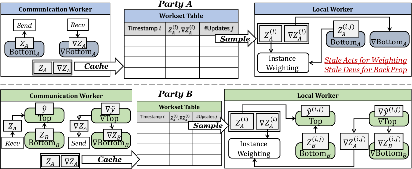
Figure 2. Overview of CELU-VFL.

3. CELU-VFL

In this section, we first introduce CELU-VFL, a novel VFL framework that enables local updates via cached statistics. Then, we propose two techniques to address the two drawbacks of local updates in VFL accordingly. We first present the frequently used notations:

• $B$: size of mini-batches;

• $R$: maximum number of updates for each mini-batch;

• $W$: size of the workset table (number of cached mini-batches);

• $\xi$: the threshold in our instance weighting mechanism;

• $Z_{A}^{(i)},\nabla Z_{A}^{(i)}$: the forward activations and backward derivatives of Party $\mathcal{A}$ of the $i$-th batch;

• $Z_{A}^{(i,j)},\nabla Z_{A}^{(i,j)}$: the forward activations and backward derivatives of Party $\mathcal{A}$ of the $i$-th batch at the $j$-th updates.

3.1. Overview

Figure 2 illustrates the overview of CELU-VFL. There are three major components, as introduced below.

The workset table is in charge of the maintenance of the cached, stale statistics. It records two “clocks” for each cached batch: (i) the timestamp when this batch is inserted, and (ii) the current number of updates done by this batch. The capacity of the table is $W$, i.e., during the insertion at time $i$, we discard cached batches inserted before time $i-W+1$ to control the maximum staleness. Whenever a cached batch is sampled for one local update, we increment the second clock correspondingly. Cached batches that reach the maximum number of updates, i.e., $R$, will be dropped as well.

The communication worker is responsible for the message transmission between parties. In the beginning, both parties agree on the ordering of mini-batches. For each batch, the communication workers execute the conventional forward and backward propagation to exchange $Z_{A}$ and $\nabla Z_{A}$. Then, both $Z_{A}$ and $\nabla Z_{A}$ are inserted into the workset table in order to execute local updates. The timestamp $i$ is set as the current number of communication rounds, i.e., the current number of processed batches.

The local worker performs local updates via the cached statistics. For each local step, the local worker of each party chooses one cached entry $\langle i,Z_{A}^{(i)},\nabla Z_{A}^{(i)},j\rangle$ from the workset table, where $i$ identifies the corresponding mini-batch and $j$ denotes how many times it has been used. Unlike FedBCD that trains on the same mini-batch for multiple consecutive steps, we exploit a round-robin local sampling strategy to reduce the stochastic variance, which will be described in Section 3.2. In addition to executing the local propagation, we develop a mechanism that weights the instances to mitigate the impact brought by staleness. For instance, as depicted in Figure 2, Party $\mathcal{A}$ feeds the stale derivatives $\nabla Z_{A}^{(i)}$ to the backward propagation process and utilizes the stale activations $Z_{A}^{(i)}$ to measure the weights of instances. We will introduce the weighting mechanism in depth in Section 3.3. Furthermore, we let the two types of workers run concurrently to make full use of both computation and communication resources.

3.2. Round-Robin Local Sampling

It is well known that stochastic optimization algorithms have inherent variance in the mini-batch gradients  (Allen-Zhu, 2017; Johnson and Zhang, 2013; Ramezani et al., 2020). As shown in Figure 3, if each mini-batch is used for consecutive steps, the stochastic variance will be accumulated and hinder the convergence. Such stochastic variance can be mitigated if we apply the mini-batches uniformly, e.g., by alternating the mini-batches. Motivated by this, we introduce a workset table that stores $W>1$ mini-batches to allow uniform local sampling. It is worthy to note that since FedBCD repetitively uses the same mini-batch for consecutive local updates, it is analogous to the simplest case of $W=1$.

Nevertheless, we observe that simply letting $W>1$ still cannot deal with the repetitive training issue. The reason is that the training workers are running too much faster than the communication workers. For instance, the top row of Figure 4 depicts a case where $W=R=3$. Whenever a mini-batch is inserted into the workset, the training worker will immediately finish the three local updates before the next mini-batch is ready. As a result, the local sampling downgrades to the repetitive training pattern.

To solve this problem, we devise a simple but effective round-robin local sampling strategy, which enforces that each mini-batch in the workset cannot be sampled again in the next $W-1$ steps. As depicted in the bottom row of Figure 4, with the round-robin strategy, the training worker samples the mini-batches one by one, guaranteeing the uniformity. Although bubbles are incurred in the first $W-1$ communication rounds, they are negligible since $W$ is far smaller than the total number of communication rounds.

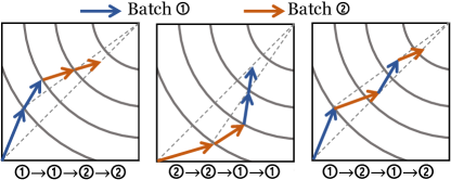
Figure 3. An illustration of the impact of mini-batches ordering. Both of the two mini-batches (indicated in blue and orange, respectively) are trained for two steps. Training in an alternating way (right-most) converges better than training in a repetitive way (left-most and middle).

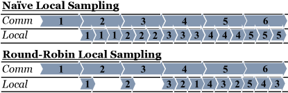
Figure 4. Naïve vs. round-robin local sampling.

Discussion. Readers might suspect that whether the convergence would be slowed down as the maximum staleness of CELU-VFL becomes $W\times R$, whilst that of FedBCD is only $R$. However, as we will analyze in Section 4.1 and evaluate in Section 5, although the round-robin strategy increases the maximum staleness, the fairness in local sampling is beneficial to convergence from two aspects. First, given the same $R$, training with $W>1$ converges faster than $W=1$. Second, CELU-VFL can support a larger $R$ whilst FedBCD diverges, so the resource utilization can be improved as well.

In addition, there are many alternatives to achieve uniform sampling, such as randomly drawing the instances inside the workset table. However, we treat each pre-determined mini-batch as a whole to be more implementation-friendly — since the mini-batches are inserted at different steps, it is easier to maintain the “clocks” of each instance. Furthermore, we can randomly shuffle the entire training dataset before training to ensure that the instances inside the workset table are also in random order.

1

2Function InsWeight($\textup{ad hoc }V^{(i,j)},\textup{stale }V^{(i)}$):

3       $weights\leftarrow\cos(V^{(i,j)},V^{(i)},axis=1)$;

4       $weights[weights<\cos\xi]\leftarrow 0$;

5       return $weights$

6Function LocalUpdatePartyA($i,Z_{A}^{(i)},\nabla Z_{A}^{(i)},j$):

7       $Z_{A}^{(i,j)}\leftarrow\textnormal{{ForwardProp}}(X_{A}^{(i)})$;

8       $ins\_weights\leftarrow\textnormal{{InsWeight}}(Z_{A}^{(i,j)},Z_{A}^{(i)})$;

9       $\textnormal{{BackwardProp}}(ins\_weights\odot\nabla Z_{A}^{(i)})$;

10      

11Function LocalUpdatePartyB($i,Z_{A}^{(i)},\nabla Z_{A}^{(i)},j$):

12       $\hat{y}^{(i,j)}\leftarrow\textnormal{{ForwardProp}}(Z_{A}^{(i)},X_{B}^{(i)})$;

13       $loss^{(i,j)}\leftarrow\textnormal{{Loss}}(y^{(i)},\hat{y}^{(i,j)},axis=1)$;

14       $\nabla Z_{A}^{(i,j)}\leftarrow\partial loss^{(i,j)}/\partial Z_{A}^{(i)}$;

15       $ins\_weights\leftarrow\textnormal{{InsWeight}}(\nabla Z_{A}^{(i,j)},\nabla Z_{A}^{(i)})$;

16       $\textnormal{{BackwardProp}}(ins\_weights\odot loss^{(i,j)})$;

17      

Algorithm 2 Procedures of local update with our instance weighting mechanism. $\cos\xi$ is a pre-defined threshold and $\odot$ denotes element-wise multiplication.

3.3. Instance Weighting Mechanism

Undoubtedly, approximation with the stale statistics causes errors in the estimated model gradients. Although there have been various works discussing that gradient optimization algorithms are robust to certain noises in gradients, the model performance will be harmed inevitably when the staleness is large. To tackle this problem, we desiderate a fine-grained mechanism that measures the reliability of each cached instance according to its staleness.

As we will analyze in Section 4.1, the convergence speed is highly related to the angles between the approximated gradients calculated using stale statistics and the expected gradients calculated using ad hoc statistics. Therefore, it is a straightforward idea to leverage the cosine similarity to measure the staleness. Nevertheless, it is impossible to calculate the expected gradients for local updates since the ad hoc statistics are not transmitted between parties, making the cosine similarity unmeasurable. Consequently, we heuristically exploit the cosine similarity measurement to the forward activations and backward derivatives, rather than the model gradients.

To be specific, our instance weighting mechanism is shown in Algorithm 2. We measure the cosine similarities between the ad hoc statistics and the stale ones, and use the similarities as instance weights. For Party $\mathcal{A}$, since the ad hoc forward activations are computed for each local update, we measure the cosine similarities by $\cos(Z_{A}^{(i,j)},Z_{A}^{(i)})$, where the cosine operation applies on every row for each instance individually. In symmetric, Party $\mathcal{B}$ measures the cosine similarities via the backward derivatives, i.e., $\cos(\nabla Z_{A}^{(i,j)},\nabla Z_{A}^{(i)})$. Furthermore, we introduce a lower bound $\cos\xi$ as the threshold, i.e., for instances whose similarities are smaller than $\cos\xi$, their weights will be set as zero. Finally, the backward propagation is executed in a weighted manner so that the model gradients will be computed in the weighted-averaged fashion.

Discussion. To help readers better understand the rationality of such a heuristic method, we use a fully connected layer $z_{out}=z_{in}\theta$ as an example, where $\theta\in\mathbb{R}^{d_{in}\times d_{out}}$ denotes the model weights and $z_{in}\in\mathbb{R}^{d_{in}},z_{out}\in\mathbb{R}^{d_{out}}$ denote the inputs and outputs of one instance, respectively. During the backward propagation, the model gradients are computed via the outer product between forward activations and backward derivatives, i.e., $\nabla\theta=z_{in}^{T}\nabla z_{out}$. For Party $\mathcal{A}$, suppose the stale derivatives are denoted as $\widetilde{\nabla}{z}_{out}$, it is easy to know that $\cos(\nabla\theta,\widetilde{\nabla}\theta)=\cos(\nabla z_{out},\widetilde{\nabla}{z}_{out})$, where $\widetilde{\nabla}\theta=z_{in}^{T}\widetilde{\nabla}{z}_{out}$. Similarly, we have the same property for Party $\mathcal{B}$. Although this is only valid for fully connected layers, it provides a hint that measuring the similarities via forward activations and backward derivatives is reasonable and achieves promising results.

4. Analysis

4.1. Convergence Analysis

When applying local updates in VFL training, we are actually solving the problem defined in Equation 1 with approximated gradients. For simplicity, we re-write it as a more general (non-convex) empirical risk minimization (ERM) problem, i.e.,

$$\min_{{\theta\in\mathbb{R}^{d}}}f(\theta)=\frac{1}{N}\sum_{k\in\mathcal{D}}f_{k}(\theta),\;{\theta}_{t+1}={\theta}_{t}-\eta{\tilde{g}}_{t}$$,

where $\eta$ is the step size and step $t$ is denoted as the number of updates. It is worthy to note that since the models of different parties may not be updated for the same number of steps due to the local update technique, the learning task in CELU-VFL can be reckoned as solving two ERM problems separately. To analyze the problem, we denote three types of gradients:

• $\nabla f(\theta_{t})=\frac{1}{N}\sum_{k\in\mathcal{D}}\nabla f_{k}(\theta_{t})$ is the full-batch gradient.

• $g_{t}=\frac{1}{B}\sum_{k\in\mathcal{B}}\nabla f_{k}(\theta_{t})$ is the mini-batch gradient of the batch $\mathcal{B}$ subsampled from the workset table $\mathcal{W}$, i.e., $\mathcal{B}\subseteq\mathcal{W}\subseteq\mathcal{D}$.

• $\tilde{g}_{t}$ is the approximated version of $g_{t}$ using stale statistics.

Compared to vanilla SGD training, the analysis in our work is more challenging due to the two drawbacks of local updates in VFL: (1. variance problem) $g_{t}$ is sampled over the workset table instead of the entire training data; (2. approximation errors) $\tilde{g}_{t}$ in local updates is approximated using the stale information, which cannot guarantee unbiasedness, i.e., $\mathbb{E}[\tilde{g}_{t}]\neq\nabla f(\theta_{t})$. Consequently, the expected errors can be dissected into two terms:

$$\small\mathbb{E}\left[\lVert\tilde{g}_{t}-\nabla f(\theta_{t})\rVert^{2}\right]\leq 2\mathbb{E}\left[\lVert g_{t}-\nabla f(\theta_{t})\rVert^{2}\right]+2\mathbb{E}\left[\lVert\tilde{g}_{t}-g_{t}\rVert^{2}\right],$$

where the first term depicts the stochastic variance due to mini-batch sampling whilst the second term comes from the approximation via stale information. Then, we make two assumptions.

Assumption 1 0.

For each step $t$, we make these two assumptions:
(1. Uniform sampling) $\mathcal{W}$ is uniformly subsampled from $\mathcal{D}$ and $\mathcal{B}$ is uniformly subsampled from $\mathcal{W}$.
(2. Correct direction) The angles between $\tilde{g}_{t},g_{t}$ are bounded, i.e., there exists a constant $\rho\in(0,1]$ s.t. $\cos(\tilde{g}_{t},g_{t})\geq\rho$.

Assumption 2 0.

For $\forall k\in\{1,2,...,N\},\theta,\theta^{\prime}\in\mathbb{R}^{d}$, we make these assumptions following Allen-Zhu (2017):
(1. $L$-Lipschitz) $\lVert{\nabla}f_{k}({\theta})-{\nabla}f_{k}({\theta^{\prime}})\rVert\leq L\lVert{\theta}-{\theta^{\prime}}\rVert$;
(2. Bounded moment) $\mathbb{E}[\lVert{\nabla}f_{k}({\theta})\rVert^{2}]\leq\sigma^{2}$;
(3. Existence of global minimum) $\exists\theta^{*}$ s.t. $f({\theta})\geq f(\theta^{*})$.

Assumption Assumption 1 ensures the unbiasedness of $\mathbb{E}[g_{t}]=\nabla f(\theta_{t})$ and guarantees that the descending directions of the approximated gradients are convincing. Assumption Assumption 2 consists of the standard assumptions widely used in the convergence analysis of stochastic optimization. We present our theoretical result in Theorem 1.

Theorem 1.

Under Assumption Assumption 1,Assumption 2 and setting the step size appropriately, after $T$ steps, select $\bar{\theta}_{T}$ randomly from $\{\theta_{t}\}_{t=0}^{T-1}$. With probability at least $1-\delta$, we have $\mathbb{E}\left[\lVert{\nabla f(\bar{\theta}_{T})}\rVert^{2}\right]\leq O(\sqrt{\Delta/T})$, where

$$\Delta=\frac{L^{2}\log\left({2d}/{\delta}\right)}{B}\left(1+\frac{1}{W}\right)+\sigma^{2}(2-\rho).$$

Remark. Note that the convergence analysis by Liu et al. (2019) relies on a strong assumption on the approximated gradients, which fails to reveal the negative impacts brought by local updates. In contrast, our analysis relies on more relaxed assumptions and uncovers the variance problem and approximation errors in local updates. This also sheds light on how the local sampling and instance weighting influence the convergence. On the one hand, with a larger $W$, the stochastic variance becomes smaller (i.e., smaller $\Delta$) and thus benefits the convergence. On the other hand, if the stale information is more reliable, which gives a higher $\rho$, the convergence would be faster as well. Nevertheless, it is worthy to notice that there exists a tradeoff since $\rho$ decreases w.r.t. $W$ and $R$ due to the larger staleness.

Communication Complexity. Compared with the sub-linear rate $O(1/\sqrt{T})$ of vanilla SGD training, our framework introduces an extra factor $O(\sqrt{\Delta})$. In other words, vanilla SGD training needs $O(T)$ steps whilst we need $O(\Delta\times T)$ steps to achieve similar convergence. However, the communication complexity of our framework can be reduced to $O(\Delta/R)$ times of that of vanilla SGD training. In Section 5, we will empirically show that CELU-VFL requires much fewer communication rounds to achieve the same model quality.

4.2. Security Analysis

Obviously, our framework shares the same security guarantees as vanilla VFL training as introduced in Section 2, since we do not need to exchange values other than activations and derivatives. We refer interested readers to the previous studies for the detailed analysis (Gu et al., 2020; Zhang et al., 2021a; Liu et al., 2019; Chen et al., 2020). Moreover, because our framework can effectively reduce the number of communication rounds as shown in our experiments, the number of messages transmitted between parties would become smaller, which conveys stronger privacy preservation.

5. Implementation and Evaluation

5.1. Setup

Implementation. We implement CELU-VFL on top of TensorFlow (Abadi et al., 2016a) and gRPC. We first develop lightweight message queues to support the send and recv primitives for cross-party communication. Then, an FLGraph abstraction is proposed to automatically generate the backward computation graph and the local update operation after the users have defined the bottom and top models. CELU-VFL has been deployed to the collaborative recommendation tasks of Tencent Inc. To be specific, Tencent works as Party $\mathcal{A}$ and provides user features, and Party $\mathcal{B}$ is an e-commercial company that owns item features and labels (such as clicks or conversions), but lacks a rich set of user features. In the preprocessing phase, the private data of both companies are aligned as user-item pairs. Then, CELU-VFL trains VFL models to fit the labels by the features of both parties.

Experimental Setup. All experiments are carried out on two servers where each server acts as one party. For each party, we run the training tasks with one NVIDIA V100 GPU. The WAN bandwidth between the two servers is 300Mbps.

Models. We focus on the deep learning recommendation models (DLRMs) since it is one of the most common neural network architectures in real-world VFL collaborations. To be specific, we consider two widely-used DLRMs, which are Wide and Deep (WDL) and Deep Structured Semantic Model (DSSM).

Table 1. Description of datasets for end-to-end evaluation.

Dataset	#Instances (train/test)	#Fields (A/B)
Criteo	41M/4.5M	26/13
Avazu	36M/4.0M	14/8
D3	32M/3.5M	25/18

Datasets. Three datasets are used in our experiments, as listed in Table 1. Criteo and Avazu are two large-scale public datasets. Whilst D3 is a productive dataset in Tencent Inc. As our major focus is the training phase, we assume all datasets have been aligned.

Protocols. We train the models using the AdaGrad optimizer (Duchi et al., 2011) with a batch size of 4096. The output dimensionality of $Z_{A}$ is set as 256. To achieve a fair comparison, we tune the learning rate for vanilla VFL training and apply the same to our work directly. For each experiment, we run three trials and report the mean and standard deviation (stddev).

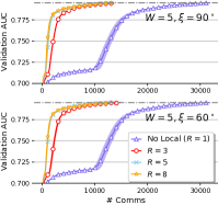
(a) Impact of local update.

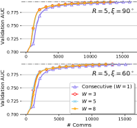
(b) Impact of local sampling.

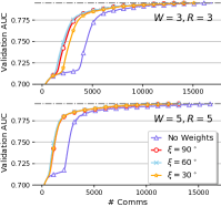
(c) Impact of instance weighting.

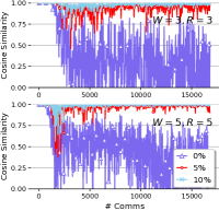
(d) Quantiles of cosine similarities.

Figure 5. Validation AUC metrics in terms of the number of communication rounds. For each technique, we conduct experiments with and without the technique and vary the corresponding hyper-parameter under two different settings.

Table 2. Number of communication rounds (mean and stddev) required to reach the same model performance in Figure 5.

Local Update	No Local $(R=1)$	$R=3$	$R=5$	$R=8$
$W=5,\xi=90^{\circ}$	$31540\pm 631.19$	$14000\pm 424.26(\downarrow 55.61\%)$	$12767\pm 654.90(\downarrow 59.52\%)$	$12733\pm 410.96(\downarrow 59.63\%)$
$W=5,\xi=60^{\circ}$	$31540\pm 631.19$	$14333\pm 329.98(\downarrow 54.56\%)$	$12767\pm 286.74(\downarrow 59.52\%)$	$12500\pm 424.26(\downarrow 60.37\%)$
Local Sampling	Consecutive $(W=1)$	$W=3$	$W=5$	$W=8$
$R=5,\xi=90^{\circ}$	$16400\pm 244.95$	$13333\pm 339.94(\downarrow 18.70\%)$	$12767\pm 654.90(\downarrow 22.15\%)$	$13333\pm 249.44(\downarrow 18.70\%)$
$R=5,\xi=60^{\circ}$	$15967\pm 339.94$	$12700\pm 141.42(\downarrow 20.46\%)$	$12767\pm 286.74(\downarrow 20.04\%)$	$12667\pm 419.00(\downarrow 20.67\%)$
Instance Weighting	No Weights	$\xi=90^{\circ}$	$\xi=60^{\circ}$	$\xi=30^{\circ}$
$W=3,R=3$	$16767\pm 492.16$	$14233\pm 235.70(\downarrow 15.11\%)$	$15200\pm 163.30(\downarrow 9.36\%)$	$14667\pm 94.28(\downarrow 12.52\%)$
$W=5,R=5$	$16467\pm 492.16$	$12767\pm 286.74(\downarrow 22.47\%)$	$12567\pm 205.48(\downarrow 23.68\%)$	$12767\pm 654.90(\downarrow 22.47\%)$

5.2. Ablation Study and Sensitivity

Compared with the vanilla VFL training, CELU-VFL contains three additional techniques, i.e., the local update technique, the uniform local sampling strategy, and the instance weighting mechanism (parameterized by $R,W,\xi$, respectively). We first investigate the impact of each technique and assess the sensitivity w.r.t. the hyper-parameters. To be specific, we train WDL on the $Criteo$ dataset and measure the number of communication rounds taken to the same target AUC metric. The convergence curves are shown in Figure 5 and the required communication rounds are listed in Table 2.

Impact of Local Update. We first assess the effect of the local update technique by varying $R$. The results are shown in Figure 5(a). In general, compared with the vanilla VFL training, applying the local update technique can significantly reduce the number of communication rounds required to reach the same model performance. For instance, when $R=3$, the number of communication rounds is reduced by around 55$\%$. When we increase $R$ to 5, the improvement increases to around 60$\%$ accordingly. Letting $R=8$ provides a faster convergence speed than that of $R=5$ in the early phase. However, due to the larger staleness, it takes a similar number of communication rounds to attain the same validation AUC.

Impact of Local Sampling. To assess the impact of the local sampling strategy, we conduct experiments with various $W$. When $W=1$, each mini-batch will be utilized for multiple consecutive local steps, whilst we apply the round-robin local sampling strategy when $W>1$ to achieve uniform sampling. As shown in Figure 5(b), the round-robin local sampling strategy consistently outperforms the consecutive counterpart — the numbers of required communication rounds are reduced by 18-22$\%$. This matches our analysis that uniform sampling can help alleviate the stochastic variance in mini-batch gradients and therefore improve the convergence. Moreover, it is worthy to note that the convergence speed does not change significantly when $W\in\{3,5,8\}$, which verifies the robustness of CELU-VFL against the choice of workset size.

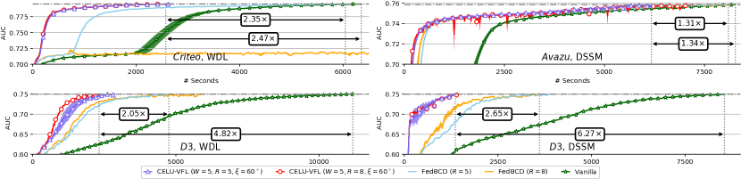
Figure 6. Validation AUC metrics in terms of running time (in seconds)

Impact of Instance Weighting. Next, we explore the benefit brought by the instance weighting mechanism with different $\xi$. The results are presented in Figure 5(c). In short, the instance weighting mechanism accelerates the convergence under both settings since it restricts the approximation errors incurred by the stale values. Under the first setting ($W=3,R=3$), we can save 9-15$\%$ of the communication rounds. Under the second setting ($W=5,R=5$), the improvement bumps to around $23\%$. This is a reasonable phenomenon — with larger $W$ and/or $R$, the staleness of cached values increases and the approximation errors are enlarged as well, so the contribution of our weighting mechanism is more significant.

We further plot the cosine similarities for better interpretability. To be specific, for each local update, we compute the quantiles of all similarities in the current batch (0% quantiles correspond to the lowest similarities). The results in Figure 5(d) show two facts: (1) Most of the stale statistics are reliable. For instance, over 90% of the cosine similarities are greater than 0.5 even in the fast converging period, which supports our motivation that the model does not change significantly and the stale statistics can be re-used in local updates. (2) Our instance weighting mechanism is able to filter or penalize the outliers to accelerate the convergence.

Summary. The experiments demonstrate the power of each technique individually. Overall, all techniques have significant contributions to reducing the number of communication rounds compared with the counterparts without the techniques. Furthermore, our work is robust to different configurations (the choices of the hyper-parameters), which is vital to the applicability in practice.

5.3. End-to-End Evaluation

Then, we evaluate the end-to-end training performance of CELU-VFL. To be specific, we compare CELU-VFL with two competitors, which are FedBCD (Liu et al., 2019) and the vanilla VFL training (denoted as Vanilla). Following the results in Section 5.2, we fix $W=5,\xi=60^{\circ}$ and let $R\in\{5,8\}$ for all experiments. We presents the convergence curves in Figure 6 and discuss the results for different datasets below.

Results on Criteo. We first train WDL on the Criteo dataset. Thanks to the reduction in communication, CELU-VFL achieves 2.47$\times$ of speedup compared with Vanilla. Whilst the performance of FedBCD is unsatisfactory. For $R=5$, although FedBCD runs faster than Vanilla in the short-term convergence, it slows down in the long-term convergence. Eventually, the gap between FedBCD and Vanilla is very small. The reason is that when the model approaches the (local) optimum point, the gradients become smaller in scale and therefore are more sensitive to the errors caused by local sampling and stale information. Worst still, FedBCD fails to converge for $R=8$ due to the large staleness. In contrast, CELU-VFL has a better statistical efficiency owing to our techniques. As a result, CELU-VFL can support a larger $R$ and outperform FedBCD by 2.35$\times$.

Results on Avazu. We then evaluate the performance by training DSSM on the Avazu dataset. First, in the early phase, both CELU-VFL and FedBCD accelerate the convergence by a large extent compared with Vanilla with the help of local updates. However, similar to the results on Criteo, FedBCD suffers from a slow convergence later, whilst CELU-VFL converges properly and achieves 1.31-1.34$\times$ of improvement compared with the other competitors.

Results on Industrial Dataset. Finally, we conduct experiments on the industrial dataset D3 to see how CELU-VFL performs in real-world workloads. Overall, CELU-VFL outperforms Vanilla by 4.82-6.27$\times$ on the two training tasks. FedBCD has a better performance on the industrial dataset, however, it is still 2.05-2.65$\times$ slower than CELU-VFL. These empirical results demonstrate the superiority of our work in practical VFL applications.

6. Related Works

Federated learning. In recent years, FL has aroused the interests from both academia and industry. Notably, VFL conveys a possibility to unite the data of different corporations and jointly build the models, which fits numerous real-world cross-enterprise collaborations  (Cheng et al., 2021; Fu et al., 2021; Yang et al., 2019b; Li et al., 2022; Hu et al., 2019). Besides VFL, another important field of FL is the horizontal FL (HFL), where the datasets are horizontally partitioned  (Yang et al., 2019a; Konečný et al., 2016a, b; Li et al., 2020b). These works are orthogonal to ours since we focus on the VFL scenario.

Asynchronous VFL. In addition to the local update technique, various works address the cross-party communication cost in VFL via asynchronous learning. However, these works cannot be applied in our scenario. Below we categorize them into two lines.

(Asynchronous Workers) The first kind of works tries to overlap computation and communication by using multiple training workers (threads) for each party (Gu et al., 2020; Zhang et al., 2021a). The models are stored in a shared-memory and each worker individually reads and updates the models in a Hogwild! manner (Recht et al., 2011). By doing so, when some workers are waiting for the message transmission, the other workers can concurrently do the computation.

Nevertheless, these methods mainly focus on linear models where the output dimensionality of the exchanged statistics is very low (e.g., only one for logistic regression and support vector machine). Due to the small message size, sending one message cannot make full use of the bandwidth, so their major bottleneck is actually the high network latency rather than the low network bandwidth. In contrast, the output dimensionality is much higher for many modern deep learning models, so the messages are much larger in size and the network bandwidth would be easily occupied when sending one message. Thus, letting multiple workers communicate concurrently would cause severe network congestion and even lead to failure. Consequently, these methods do not fit our scenario.

(Asynchronous Parties) The second category assumes that there are two or more Party $\mathcal{A}$’s and allows different parties to train asynchronously (Chen et al., 2020; Hu et al., 2019). To be specific, Party $\mathcal{B}$ is treated as a server that holds the labels and stores the forward activations received from all Party $\mathcal{A}$’s. During the training process, each Party ${\mathcal{A}_{i}}$ individually samples a mini-batch and sends $Z_{A_{i}}$ to Party $\mathcal{B}$. Upon receiving, Party $\mathcal{B}$ updates the local storage, computes and returns $\nabla Z_{A_{i}}$. Finally, each Party ${\mathcal{A}_{i}}$ individually performs a backward propagation to update $\theta_{Bot\_{A_{i}}}$ without synchronizing with other parties. The spirit of this line of research lies with the asynchrony between Party $\mathcal{A}$’s — different Party $\mathcal{A}$’s can train on different mini-batches to achieve asynchronous learning.

However, such methods are orthogonal to our work since we focus on the case where only one Party $\mathcal{A}$ is involved, which is more commonly seen in real-world applications. Moreover, since these works still require to exchange forward activations and backward derivatives in every step, our work can be integrated with their methods easily by applying the local update technique for each Party ${\mathcal{A}_{i}}$ individually. We would like to leave the extension to multi-party VFL training as our future work.

7. Conclusion

This paper focuses on the deficiency caused by heavy cross-party communication in VFL training. Specifically, we propose CELU-VFL, an efficient VFL training framework with cached-enable local updates. To improve the statistical efficiency, we develop two novel techniques to achieve fairness in stale statistics sampling and measure the fine-grained reliability of the local updates, respectively. Finally, both theoretical analysis and empirical experiments verify the effectiveness of CELU-VFL.

Appendix A Proofs

This section provides proofs for the analysis in our paper.

We first introduce an importance lemma that constitutes a non-asymptotic bound for sampling.

Lemma 1.

[Lemma 10 of Ramezani et al. (2020)] Let the subsampled function defined as

$$F_{\mathcal{S}}(x)=\frac{1}{S}\sum_{k\in\mathcal{S}}F_{k}(x),\mathbb{E}\left[{F_{\mathcal{S}}(x)}\right]=F(x),$$

where $S=\left|\mathcal{S}\right|$ and $F_{k}(x)\in\mathbb{R}^{d}$ is $L$-Lipschitz continuous for all $k$. For $\varepsilon\leq 2L$, we have with probability at least $1-\delta$ that

$$\left\lVert{F_{\mathcal{S}}(x)-F(x)}\right\rVert\leq 4\sqrt{2}L\sqrt{\frac{\log(2d/\delta)+1/4}{S}}.$$

Based on Lemma 1, we introduce the following lemma that provides an upper bound on the stochastic variance.

Lemma 2.

Under Assumption Assumption 1 and Assumption Assumption 2, for each step $t$, with probability at least $1-\delta$, we have

$$\mathbb{E}\left[{\left\lVert{{\tilde{g}}_{t}-\nabla f(\theta_{t})}\right\rVert^{2}}\right]\leq O\left(\frac{L^{2}\log\left({2d}/{\delta}\right)}{B}\left(1+\frac{1}{W}\right)+\sigma^{2}(2-\rho)\right).$$

Proof.

For simplicity, we omit the subscript of step $t$ in the proof. Since the inequality $\left\lVert{x+y}\right\rVert^{2}\leq 2\left\lVert{x}\right\rVert^{2}+2\left\lVert{y}\right\rVert^{2}$ holds, we only need to prove two claims.

Claim 1.

Under the uniform sampling assumption and the Lipschitz assumption (Assumption Assumption 1(1) and Assumption Assumption 2(1)), with probability at least $1-\delta$, we have

$$\mathbb{E}\left[{\left\lVert{g-\nabla f(\theta)}\right\rVert^{2}}\right]\leq O\left(\frac{L^{2}\log\left({2d}/{\delta}\right)}{B}\left(1+\frac{1}{W}\right)\right).$$

Proof of Claim 1.

Since $g$ is computed over a mini-batch $\mathcal{B}$ subsampled from the workset $\mathcal{W}$, by denoting the gradients over $\mathcal{W}$ as ${\bar{g}}=\frac{1}{WB}\sum_{k\in\mathcal{W}}\nabla f(\theta)$, we have

$$\mathbb{E}_{\mathcal{B}\sim\mathcal{W}}[g]={\bar{g}},\;\mathbb{E}_{\mathcal{W}\sim\mathcal{D}}[{\bar{g}}]=\nabla f(\theta).$$

Based on the $L$-Lipschitz assumption on $\nabla f$ and Lemma 1, with probability at least $1-\delta$, we have

$$\left\lVert{g-{\bar{g}}}\right\rVert =\left\lVert{\frac{1}{B}\sum_{k\in\mathcal{B}}\nabla f_{k}(\theta)-\mathbb{E}_{\mathcal{B}\sim\mathcal{W}}\left[\frac{1}{B}\sum_{k\in\mathcal{B}}\nabla f_{k}(\theta)\right]}\right\rVert$$

$$\leq 4\sqrt{2}L\sqrt{\frac{\log(2d/\delta)+1/4}{B}},$$

and

$$\left\lVert{{\bar{g}}-\nabla f(\theta)}\right\rVert =\left\lVert{\frac{1}{WB}\sum_{k\in\mathcal{W}}\nabla f_{k}(\theta)-\mathbb{E}_{\mathcal{W}\sim\mathcal{D}}\left[\frac{1}{WB}\sum_{k\in\mathcal{W}}\nabla f_{k}(\theta)\right]}\right\rVert$$

$$\leq 4\sqrt{2}L\sqrt{\frac{\log(2d/\delta)+1/4}{WB}},$$

Denoting $\mathbb{E}_{\mathcal{W}\sim\mathcal{D}}\left[\mathbb{E}_{\mathcal{B}\sim\mathcal{W}}\left[\cdot\right]\right]$ as $\mathbb{E}\left[\cdot\right]$ for simplicity, with probability at least $1-\delta$, we have

$$\mathbb{E}\left[\left\lVert{g-\nabla f(\theta)}\right\rVert^{2}\right] \leq 2\mathbb{E}\left[\left\lVert{g-{\bar{g}}}\right\rVert^{2}\right]+2\mathbb{E}\left[\left\lVert{{\bar{g}}-\nabla f(\theta)}\right\rVert^{2}\right]$$

$$\leq\frac{64L^{2}\left(\log\left({2d}/{\delta}\right)+{1}/{4}\right)}{B}\left(1+\frac{1}{W}\right).$$

Given that $2d/\delta\gg e^{1/4}$, we have

$$\mathbb{E}\left[\left\lVert{g-\nabla f(\theta)}\right\rVert^{2}\right]\leq O\left(\frac{L^{2}\log\left({2d}/{\delta}\right)}{B}\left(1+\frac{1}{W}\right)\right)$$

This completes the proof of Claim 1. ∎

Claim 2.

Under the correct direction assumption and the bounded moment assumption (Assumption Assumption 1(2) and Assumption Assumption 2(2)), we have

$$\mathbb{E}\left[{\left\lVert{{\tilde{g}}-g}\right\rVert^{2}}\right]\leq\sigma^{2}(2-\rho).$$

Proof of Claim 2.

The correct direction assumption implies

$$\left\lVert{{\tilde{g}}-g}\right\rVert^{2} =\left\lVert{{\tilde{g}}}\right\rVert^{2}+\left\lVert{g}\right\rVert^{2}-2\left\langle{{\tilde{g}}},{g}\right\rangle$$

$$=\left\lVert{{\tilde{g}}}\right\rVert^{2}+\left\lVert{g}\right\rVert^{2}-2\cos({\tilde{g}},g)\left\lVert{{\tilde{g}}}\right\rVert\left\lVert{g}\right\rVert$$

$$\leq\left\lVert{{\tilde{g}}}\right\rVert^{2}+\left\lVert{g}\right\rVert^{2}-2\rho\left\lVert{{\tilde{g}}}\right\rVert\left\lVert{g}\right\rVert$$

$$=(1-\rho)(\left\lVert{{\tilde{g}}}\right\rVert^{2}+\left\lVert{g}\right\rVert^{2})+\rho(\left\lVert{{\tilde{g}}}\right\rVert-\left\lVert{g}\right\rVert)^{2}.$$

Since the norms of gradients ($\left\lVert{{\tilde{g}}}\right\rVert$ and $\left\lVert{g}\right\rVert$) are non-negative, the inequality $(\left\lVert{{\tilde{g}}}\right\rVert-\left\lVert{g}\right\rVert)^{2}\leq\max\left\{\left\lVert{{\tilde{g}}}\right\rVert^{2},\left\lVert{g}\right\rVert^{2}\right\}$ holds. Therefore,

$$\left\lVert{{\tilde{g}}-g}\right\rVert^{2} \leq(1-\rho)(\left\lVert{{\tilde{g}}}\right\rVert^{2}+\left\lVert{g}\right\rVert^{2})+\rho(\left\lVert{{\tilde{g}}}\right\rVert-\left\lVert{g}\right\rVert)^{2}$$

$$\leq 2(1-\rho)\max\left\{\left\lVert{{\tilde{g}}}\right\rVert^{2},\left\lVert{g}\right\rVert^{2}\right\}+\rho\max\left\{\left\lVert{{\tilde{g}}}\right\rVert^{2},\left\lVert{g}\right\rVert^{2}\right\}$$

$$=(2-\rho)\max\left\{\left\lVert{{\tilde{g}}}\right\rVert^{2},\left\lVert{g}\right\rVert^{2}\right\}.$$

Combining with the bounded moment assumption, we have

$$\mathbb{E}\left[{\left\lVert{{\tilde{g}}-g}\right\rVert^{2}}\right]\leq\sigma^{2}(2-\rho).$$

This completes the proof of Claim 2. ∎

Finally, combining Claim 1, Claim 2 and the inequality that $\left\lVert{x+y}\right\rVert^{2}\leq 2\left\lVert{x}\right\rVert^{2}+2\left\lVert{y}\right\rVert^{2}$, we complete the proof of Lemma 2. ∎

Next, we present the proof for Theorem 1.

Theorem 1.

Under Assumption Assumption 1,Assumption 2 and setting the step size appropriately, after $T$ steps, select $\bar{\theta}_{T}$ randomly from $\{\theta_{0},\theta_{1},\dots,\theta_{T-1}\}$. With probability at least $1-\delta$, we have

$$\mathbb{E}\left[\lVert{\nabla f(\bar{\theta}_{T})}\rVert^{2}\right]\leq O\left(\sqrt{{\left(\frac{L^{2}\log\left({2d}/{\delta}\right)}{B}\left(1+\frac{1}{W}\right)+\sigma^{2}(2-\rho)\right)}/{T}}\right).$$

Proof.

By Taylor’s Expansion Formula with Lagrangian Remainder, we have

$$f(\theta_{t+1}) =f(\theta_{t}-\eta{\tilde{g}}_{t})$$

$$\leq f(\theta_{t})-\eta\left\langle{{\tilde{g}}_{t}},{\nabla f(\theta_{t})}\right\rangle+\frac{L}{2}\eta^{2}\left\lVert{{\tilde{g}}_{t}}\right\rVert^{2}$$

$$=f(\theta_{t})-\eta\left\langle{\nabla f(\theta_{t})+{\tilde{g}}_{t}-\nabla f(\theta_{t})},{\nabla f(\theta_{t})}\right\rangle+\frac{L}{2}\eta^{2}\left\lVert{{\tilde{g}}_{t}}\right\rVert^{2}$$

$$=f(\theta_{t})-\eta\left\lVert{\nabla f(\theta_{t})}\right\rVert^{2}-\eta\left\langle{{\tilde{g}}_{t}-\nabla f(\theta_{t})},{\nabla f(\theta_{t})}\right\rangle$$

$$\;\;\;+\frac{L}{2}\eta^{2}\left\lVert{{\tilde{g}}_{t}}\right\rVert^{2},$$

where the first inequality is due to the property of Lipschitz continuity. By substituting $\left\lVert{{\tilde{g}}_{t}}\right\rVert^{2}$ as

$$\left\lVert{{\tilde{g}}_{t}}\right\rVert^{2} =\left\lVert{{\tilde{g}}_{t}-\nabla f(\theta_{t})+\nabla f(\theta_{t})}\right\rVert^{2}$$

$$=\left\lVert{{\tilde{g}}_{t}-\nabla f(\theta_{t})}\right\rVert^{2}+\left\lVert{\nabla f(\theta_{t})}\right\rVert^{2}+2\left\langle{{\tilde{g}}_{t}-\nabla f(\theta_{t})},{\nabla f(\theta_{t})}\right\rangle,$$

we have

$$f(\theta_{t+1}) \leq f(\theta_{t})+(L\eta^{2}-\frac{3}{2}\eta)\left\lVert{\nabla f(\theta_{t})}\right\rVert^{2}$$

$$\;\;\;+(L\eta^{2}-\frac{1}{2}\eta)\left\lVert{{\tilde{g}}_{t}-\nabla f(\theta_{t})}\right\rVert^{2}$$

$$\leq f(\theta_{t})+(L\eta^{2}-\frac{3}{2}\eta)\left\lVert{\nabla f(\theta_{t})}\right\rVert^{2}$$

$$\;\;\;+L\eta^{2}\left\lVert{{\tilde{g}}_{t}-\nabla f(\theta_{t})}\right\rVert^{2}.$$

Taking expectation on both sides, we have

$$(\frac{3}{2}\eta-L\eta^{2})\mathbb{E}\left[{\left\lVert{\nabla f(\theta_{t})}\right\rVert^{2}}\right] \leq\mathbb{E}\left[{f(\theta_{t})}\right]-\mathbb{E}\left[{f(\theta_{t+1})}\right]$$

$$\;\;\;+L\eta^{2}\mathbb{E}\left[{\left\lVert{{\tilde{g}}_{t}-\nabla f(\theta_{t})}\right\rVert^{2}}\right]$$

Summing over $T$ steps and dividing both sides by $(\frac{3}{2}\eta-\eta^{2}L)T$, and noticing that $\bar{\theta}_{T}$ is selected randomly from $\{\theta_{0},\theta_{1},\dots,\theta_{T-1}\}$, we have

$$\mathbb{E}\left[{\left\lVert{\nabla f(\bar{\theta}_{T})}\right\rVert^{2}}\right] =\frac{1}{T}\sum_{t=0}^{T-1}\mathbb{E}\left[{\left\lVert{\nabla f(\theta_{t})}\right\rVert^{2}}\right]$$

$$\leq\frac{2}{(3\eta-L2\eta^{2})T}(f(\theta_{0})-\mathbb{E}[f(\theta_{t})])$$

$$\;\;\;+\frac{2L\eta}{(3-2L\eta)T}\sum_{t=0}^{T-1}\mathbb{E}\left[{\left\lVert{{\tilde{g}}_{t}-\nabla f(\theta_{t})}\right\rVert^{2}}\right]$$

$$\leq\frac{2}{(3\eta-L2\eta^{2})T}(f(\theta_{0})-f(\theta^{*}))$$

$$\;\;\;+\frac{2L\eta}{(3-2L\eta)T}\sum_{t=0}^{T-1}\mathbb{E}\left[{\left\lVert{{\tilde{g}}_{t}-\nabla f(\theta_{t})}\right\rVert^{2}}\right]$$

Denote $V=\frac{1}{T}\sum_{t=0}^{T-1}\mathbb{E}\left[{\left\lVert{{\tilde{g}}_{t}-\nabla f(\theta_{t})}\right\rVert^{2}}\right]$. According to Lemma 2, $V\leq O\left(\frac{L^{2}\log\left({2d}/{\delta}\right)}{B}\left(1+\frac{1}{W}\right)+\sigma^{2}(2-\rho)\right)$ satisfies with probability at least $1-\delta$. Therefore, letting $\eta=\min\left\{\frac{3}{2L},\sqrt{\frac{f(\theta_{0})-f(\theta^{*})}{LTV}}\right\}$, we have

$$\mathbb{E}\left[{\left\lVert{\nabla f(\bar{\theta}_{T})}\right\rVert^{2}}\right] \leq\frac{2(f(\theta_{0})-f(\theta^{*}))}{(3\eta-L2\eta^{2})T}+\frac{2L\eta V}{(3-2L\eta)}\leq O\left(\sqrt{\frac{V}{T}}\right)$$

$$\leq O\left(\sqrt{\frac{\frac{L^{2}\log\left({2d}/{\delta}\right)}{B}\left(1+\frac{1}{W}\right)+\sigma^{2}(2-\rho)}{T}}\right).$$

∎