A Graph Theoretic Exploration of Coronary Vascular Trees

Abstract

The aim of this study was to automate the generation of small coronary vascular networks from large point clouds that represent the coronary arterial network. Smaller networks that can be generated in a predictable manner can be used to assess the impact of network morphometry on, for example, blood flow in hemodynamic simulations. We develop a set of algorithms for generating coronary vascular networks from large point clouds. These algorithms sort the point cloud, simplify its network structure without information loss, and produce subgraphs based on given, physiologically meaningful parameters. The data were originally collected from optical fluorescence cryomicrotome images and processed before their use here.

Keywords Coronary  $\cdot$ Vascular  $\cdot$ Modelling  $\cdot$ Reconstruction

1 Introduction

The beating of the heart drives blood throughout the body via the systemic and pulmonary circulatory systems, and to itself via the coronary circulation. The proper function is essential to life, as such coronary hemodynamics is an area of great and growing research interest. Hemodynamic modeling studies can prove to be a cost-effective avenue to gaining greater insight into, for example, hypertension, vascular rarefaction, and microvascular stiffening. However, detailed vascular morphometric knowledge is vital when attempting to accurately model the hemodynamics of any organ system (Chambers et al., 2020; Nordsletten et al., 2006; van Bavel and Spaan, 1992; Hyde et al., 2014; Müller and Toro, 2014; Mynard et al., 2014; Mynard and Smolich, 2016; Qureshi et al., 2014; Olufsen et al., 2012).

There is a high degree of similarity between porcine and human coronary anatomy and hemodynamics (Lelovas et al., 2014). Hence, studying the porcine coronary system can be a useful model of the human coronary system. In both pigs and humans, the heart is comprised of four chambers: left and right atria at the top, and left and right ventricles at the bottom. Deoxygenated blood travels to the lungs from the right ventricle and through the pulmonary venous system and to the pulmonary capillaries where it is oxygenated; from here, the oxygenated blood travels through the pulmonary arteries to the left atrium and into the left ventricle. From the left ventricle, oxygenated blood is pumped into the systemic circulation via the aorta. The systemic arterial circulation supplies all organs apart from the lungs with blood, and the systemic venous system returns deoxygenated blood to the right atrium. From the right atrium, blood passes into the right ventricle where the cycle continues. The coronary circulatory system supplies the heart wall with blood; its main arteries branch from the aorta slightly distal to the aortic valve. By and large, the left coronary artery gives rise to vessels that supply the left atrium and ventricle, and similarly for the right. The left ventricle is large than the right, so it is to be expected that the left coronary arterial tree is large than the right, giving rise to two large vessels: the left anterior descending (LAD) and left circumflex arteries (LCx). Coronary artery anomalies are rare in humans (Ogden, 1970; Yildiz et al., 2010; Yamanaka and Hobbs, 1990; Kardos et al., 1997), with the vast majority of the population sharing the major branches. This is not true of minor arterial branches: as with other vascular systems, smaller vessels exhibit a greater range of morphometry. Given this variation, it may be dubious to ascribe the conclusions made by analysing hemodynamic insights gained from simulations in trees built from aggregate data, such as presented by Kassab et al. (1993, 1994) to individuals, and instead one must use patient-specific data. However, arterial trees are comprised of many thousands of vessels; too many vessels to hope to explicitly model blood flow in each explicitly in a time-effective manner. Here, we describe our process of post-processing a data set that represents the coronary arterial network of a single pig to build coronary arterial trees to use in 1D hemodynamic studies. One of the aims of these studies was to investigate the impact that post-processing makes to simulated hemodynamics (Mackenzie, 2021).

2 Materials & Methods

2.1 Raw Data

The raw data discussed here were shared with the authors by collaborators and are discussed by Goyal et al. (2012); they briefly discuss the animal preparation, data collection, and post-processing, as do Hyde et al. (2014) and Sinclair et al. (2015). More detailed discussions of materials and methods can be found in the original literature (van Horssen et al., 2009; van den Wijngaard et al., 2011). We treat the data collection and processing methods as a black box.

The data consists of a point cloud that represents a partial left coronary arterial tree. It contains 17945 nodes each with an associated 3D Cartesian coordinate, radius, and neighbour nodes. The tree is incomplete due to constraints in data collection and image processing techniques.

2.2 Obtaining a Connected Graph

The collection of nodes and edges that represent the coronary arterial tree is a disconnected, simple, directed graph. There is a large connected network that consists of all but 41 of the nodes; the disconnected nodes were found using Dijkstra’s algorithm and are discarded.

2.3 Node Types and Edge Properties

By construction, all nodes in the tree are connected to one, two, or more than two other nodes. Nodes with only one connection are called terminal, nodes with two connections are body, and nodes with more than two connections are junction nodes. Terminal nodes lie at the end of the branches of the graph; body nodes lie between junction nodes. There are 1994 terminal nodes, 13993 body nodes, and 1917 junction nodes in the tree. Body nodes do not affect the structure of the tree, but the 3D space that it occupies. We create collections of body nodes that lie between two junctions or a junction and a terminal node into segments. A lateral view of the segments of the tree are shown in Fig. 1(a). The graph theoretic problem of analysing the structure of the tree can be significantly simplified by considering only the junction and terminal nodes, along with the segments.

Rendering 3D spatial data in a 2D medium may lead to difficulty in the interpretation of the figures. In order to curtail such issues, it is reasonable to choose a consistent 2D projection for the data. Henceforth we use a Mercator projection (Miller, 1942) that preserves the branching structure of the tree but not the length of the segments. The Mercator projection of the segments is shown in Fig. 1(b).

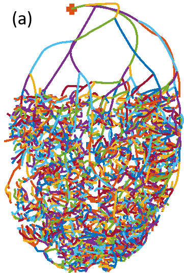
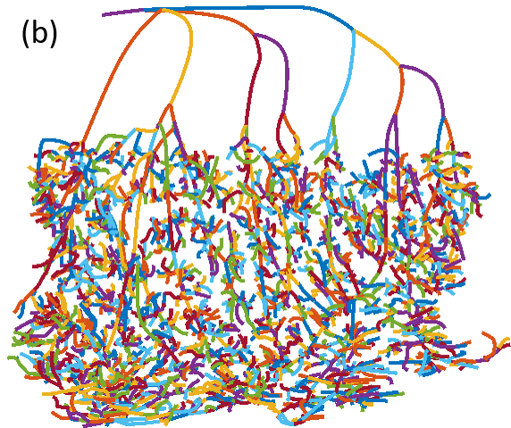
Figure 1: Segments of the vascular tree. Line colour demarcates the segments. (a) Lateral view of the segments of the vascular tree. The root node is marked with a red plus. (b) Mercator projection of the segments of the vascular tree.

Physiologically, coronary arterial flow is mostly one-directional (Mackenzie, 2021), so it is reasonable to endow the segments with an orientation to make a directed graph. The root node is chosen by visual inspection of the data to be the one highest in the tree. It is marked in Fig. 1(a).

Segments can be generated by choosing an inlet node and running Dijkstra’s algorithm (Dijkstra, 1959) to find paths from the root to all terminal nodes in the tree. This gives a path from the root to a given terminus. These paths can be split at junction nodes to give paths between a junction and a junction or a terminus – these are precisely segments. As the collection of paths spans the tree, so does the collection of segments.

2.4 Filtration and Pruning

Due to the size of the data set, the application of organisational methods to the data is essential to gaining insight into the stricture and creating subtrees that are useful in applications such as hemodynamic simulations. Here, we discuss the application of sorting and filtration methods to the 3910 segments. Filters are used to select segments that are eligible for inclusion in a final subtree. The whole tree is pruned to create subtrees that, typically, contain many fewer segments than the original tree but that are small enough to be understood by the reader.

In all pruning techniques, a threshold is set on one or more of the attributes of a segment. If a given segment surpasses these, then it is eligible for inclusion in the final tree. Pruning may result in a disconnected tree. If this is the case, then either the disconnected segments should be removed, they should be reattached to the main tree by including the intervening segments, or some combination of the two. Removing disconnected segments is most straightforward, and results in smaller trees than the latter two; it is the method employed here. The process of discarding members from a set of filtered segments is called pruning. There are many possible tree prunings, not all of which produce unique trees.

2.4.1 Radius Based Filtration

Each segment contains at least two nodes. Each of these nodes has an associated radius. In radius-based pruning, a radius threshold is given. The radii in this coronary tree are not monotonically decreasing, so applying a radius-based pruning condition is not as straightforward as finding the segments that contain a node that exceeds the threshold. There are several possible ways to apply a radius-based pruning condition. Here, we discuss a mean radius condition, a proportional condition, and a single node condition.

Mean Radius

In a mean radius condition, each segment is considered individually, and if the mean radius of nodes in that segment exceeds some threshold then the segment is eligible for inclusion in the final tree. This method may be sensitive to spurious radius values that skew the distribution for a vessel. Comparing, for example, the mean and median radius in each segment may highlight segments in which this is an issue. This is outwith the scope of the current analysis. A mean-radius filtered tree can be seen in Fig. 2(a).

Proportional Threshold

If a certain proportion of nodes in a segment have a radius greater than the given threshold, then that segment is eligible for inclusion in the final tree. This condition may be ill-suited to dealing with segments that contain few nodes. Other radius-based conditions exist, and it is certainly possible to apply multiple conditions within a single tree based on, for example, segment length. Such combinations are outwith the scope of this analysis. A proportional-threshold filtered tree can be seen in Fig. 2(b).

Single Node

If a single node in a segment has an associated radius that exceeds some threshold, then it is eligible for inclusion in the final tree. Including any segment with at least one node with a radius that surpasses some threshold will lead to the inclusion of more vessels than the above-described mean radius condition. However, it will be less sensitive to the existence of spuriously small radii values. A single node filtered tree can be seen in Fig. 2(c).

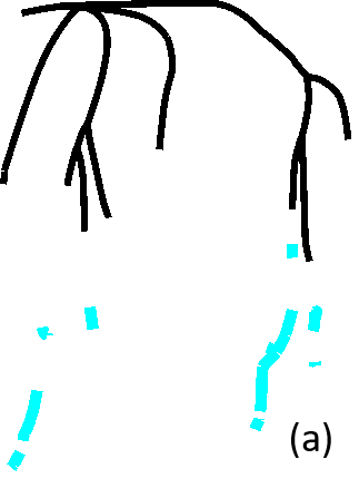
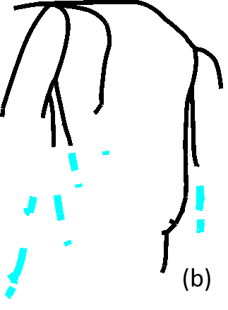
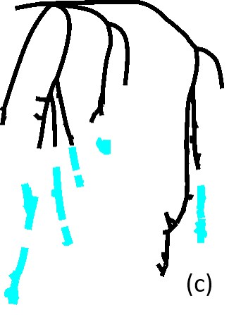
Figure 2: Radius filtered and pruned trees with a threshold set at 0.6 mm. Connected subtrees are shown in solid black and disconnected segments in cyan. (a) The mean radius condition is applied; there are 47 connected segments and 21 disconnected. (b) A proportion threshold is set to 0.8 and applied; there are 26 connected segments and 21 disconnected. (c) A single point threshold is applied to yield a connected tree of 75 connected segments and 53 disconnected.

2.4.2 Generation Assignation

The collection of segments can be hierarchically ordered according to the generation to which they belong. Generation affiliation can be used as a filter for segments. In order to apply such a filter, it is necessary to sort the nodes into generations. The 0-th generation contains only the segment that contains the inlet node. Given $i$ sorted generations, the $(i+1)$-th generation contains segments that begin with the final nodes of the $i$-th generation. It is possible to sort any subset of segments into generations.

The 3910 segments discussed here can be sorted into 42 generations. A projection of the first four generations is shown in Fig. 3(a). It is surprising that there appear to be three segments that arise directly from the $0$-th generation, but these segments belong to the 1-st and 2-nd generations; this indicates that there is a vessel in the 1-st generation that is too small to see. This short segment can be clearly seen in Fig. 3(b) with 30 times magnification centered at the first junction. The short segment contains only two nodes, while its sibling contains 51 nodes, and its daughters contain 9 and 39 nodes. Further, the radii at both nodes of the segment are greater than its length. Given this, it is reasonable to presume that the short segment is an artifact of the data collection and processing techniques. In effect, a trifurcation is captured by two bifurcations in quick succession. We call such a junction a pseudo-trifurcation. It is possible to replace pseudo-trifurcations (or indeed higher order junctions) with trifurcations by replacing the initial node in all daughters of the short segment with the initial node of the short segment, in effect not taking a path through the second bifurcation point. Figure 3(c) shows the $(x,y)$-plane projection of the first four generations of the tree without the short segment. Note that all the apparent daughters of the black inlet segment belong to the same generation. Figure 3(d) shows the initial junction at 30 times magnification without the short segment.

All segments containing only two nodes are assumed to be artifacts. Given this, we seek to remove all pseudo-trifurcations as described above. We find that there are 761 such short segments are removed, and the number of generations in the tree is reduced to 31.

To remove a pseudo-trifurcation, either the trifurcation point can be moved up (the initial bifurcation point is chosen as the trifurcation point) or moved down (the second bifurcation point is chosen). The choice does not impact the branching structure of the final tree but does impact how it occupies space, i.e. branching angles and volume may be altered. For pseudo-trifurcations, it is easy to choose the second bifurcation point to be the trifurcation point. A long segment may give rise to one or more short segments, and the short segments may in turn give rise to one or more short segments. There are many possible combinations of branching structures that involve short segments. In all cases, short segments are easy to remove by moving the bifurcation point up. In a pseudo-trifurcation involving a single short segment, it is easy to move the junction point down, but this becomes much harder when there is more than one short segment, as there is no obvious choice of junction point. Hence, in the interests of ease of automation, we choose always to move the point up.

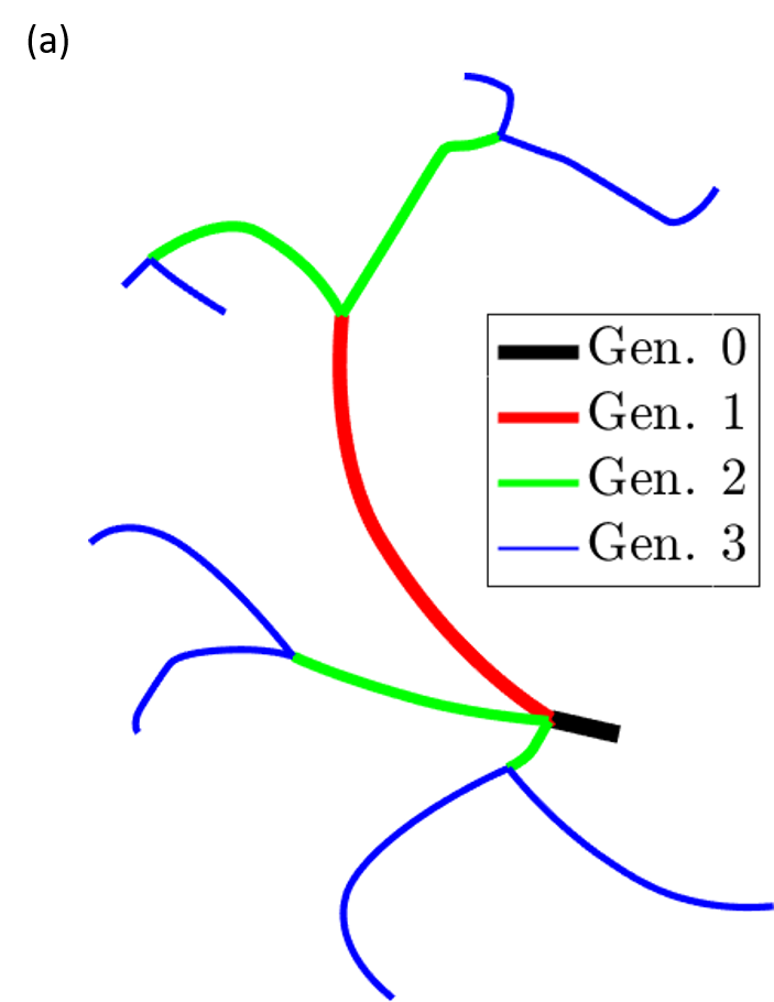
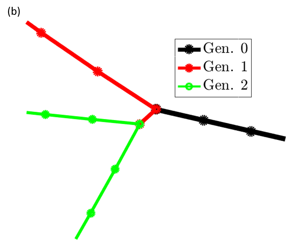
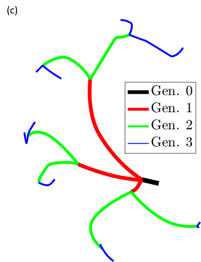
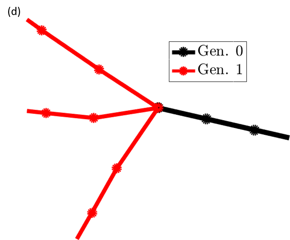
Figure 3: Segments are sorted into generations and shown in a $(x,y)$-plane projection. Line weight and colour signify generation affiliation. (a) All segments are sorted into generations without modification. (b) 30-fold magnification of the initial junction in the tree shown in $a$; spatial nodes are highlighted with circles and the short segment is clear to see. (c) Pseudo-trifurcations are removed and the resulting tree is shown with the same view as $a$. (d) as in $b$, but in the tree without pseudo-trifurcations.

2.4.3 Strahler Ordering

The Strahler order of a tree is a metric of its branching complexity. The metric was first developed by Horton (1945) and later by Strahler (1952, 1957) for applications in hydrology. Strahler ordering has been widely applied to vascular trees, see, for example, Jiang et al. (1994); Nordsletten et al. (2006); Schwen and Preusser (2012); van Bavel and Spaan (1992). Strahler numbers are assigned in a bottom-up fashion as follows:

1. if a branch has no children, it is given order 1

2. if a branch has a child of order $n$ and all other children have order less than $n$, then give the branch order $n$

3. if the branch has two or more children of order $n$, and no children with greater order, the Strahler order is $n+1$

The Strahler order of the tree discussed here is 7. Kassab et al. (1993) find the Strahler order of the left porcine coronary arterial tree to be 11. In their corrosion casting study, Kassab et al. (1993) captured images of vessels with radii in the range 4.23 $\mathrm{\SIUnitSymbolMicro m}$ – 1.7 $\mathrm{mm}$. The radius range in the data discussed here is 103.5 $\mathrm{\SIUnitSymbolMicro m}$ – 1.7 $\mathrm{mm}$. We conclude that the discrepancy in the Strahler order of the trees arises from the lower resolution of the data discussed here; indeed they record the length and diameter of more than 8000 segments in a summary table of the porcine left anterior descending artery, not including the left circumflex artery as a subtree.

Figure 4 shows the largest segments of the tree that belong to orders 3 – 7. Vessels of orders 1 and 2 are omitted as they are sufficiently numerous to occlude other vessels in the tree.

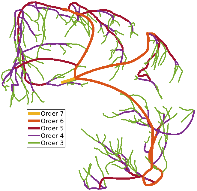
Figure 4: Segments of the vascular tree with Strahler orders 3 – 7. Line weight and color indicate the order to which a vessel belongs.

2.5 Further Pruning

The application of the desired filters to the tree may result in a connected subgraph, however, this is often not the case and further cleaning is needed to generate usable and useful trees. This section addresses the techniques applied to a filtered or pruned subtree to generate further subtrees that better meet the users’ needs.

2.5.1 Removing Disconnected Segments

Some filtration methods result in collections of segments that do not form a connected graph. In particular, this occurs in radius-based filtration when the radii within the tree are not monotonically decreasing. Most of the use cases for the trees produced with the analysis discussed here require a connected network.

There are at least two possible approaches to removing disconnected segments: remove the disconnected components from the subtree, or build a new subtree using only the connected components of the one to be cleaned. If properly implemented, these should result in the same network, but their implementations do differ. The latter is straightforward if the segments have already been sorted into their generations. Connected subtrees of non-connected subtrees are generated by comparing the two subsequent generations with a top-down approach. Starting from $i=0$, check if the daughters of the $i$-th generation are in the non-connected tree, they should be added to the growing connected tree. The collection of connected daughters of the $i$-th generation forms the $(i+1)$-th generation. Repeat this step until all generations have been parsed. This is the procedure used to remove the segments highlighted in cyan seen in Figs. 2.

2.5.2 Setting a Maximum Number of Generations

One possible application of the trees generated using the current analysis is in hemodynamic flow models. In these, there is a trade-off between model fidelity and computational cost. Flow simulations in trees with more branches are more computationally costly than those with fewer branches, not just because of the branch count itself, but because the junctions between vessels can be expensive to match (Mackenzie, 2021). In two-sided models such as those discussed by Mackenzie (2021) and Qureshi et al. (2014), a single additional generation of vessels can as much as quadruple computational costs (Mackenzie, 2021). As shown by Mackenzie (2021), the flow in all vessels is correlated to the total volume of the network. In the tree, segment volume typically decreases as a function of increasing distance from the inlet. In this tree, the number of vessels per generation is increasing until the 16-th generation and contains a total of 1927 segments. Given all this, it is reasonable to ask what the maximum number of generations that ought to be included in the tree is. One possible metric that can be used to help answer this question is the information density, $I$. Let $n$ be the number of segments per generation and $v$ be the total volume of the segments in a generation. Generations are indexed by a non-negative integer $i$. Information density is defined to be the ratio $I:=v/n$. Figure 5 shows graphs of $n$, $v$, and $I$ as discrete functions of $i$. Information density has a peak when $i=2$ and decreasingly decreasing from then on. The additional information gained by adding another generation can be quantified by finding $\Delta I=I(n+1)-I(n)$ for $n\geq 0$. This peaks at $i=0$, between the 0-th and 1-st generations. Let the threshold on $\Delta I$ for excluding a generation be two orders of magnitude lower than its peak, i.e. all generations after the first for which

$$|\Delta I(i)|<\frac{{\rm max}(\Delta I)}{100}$$

holds should not be included. This happens first when $i=5$. If one wishes to use a generation-based filter to reduce the number of segments eligible for inclusion in a tree, a reasonable choice for an upper bound based on this metric is 5.

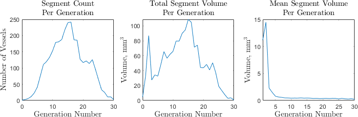
Figure 5: Plots of the segments count, volume, and volume-to-count ratio per generation.

Figure 6(a) shows the Mercator projection of the first six generations of segments, while Fig. 6(b) shows the connected tree of segments in the first six generations that have a mean radius greater than 0.6mm. Generations 0 – 5 contain 162 segments, 28 of which meet the radius condition.

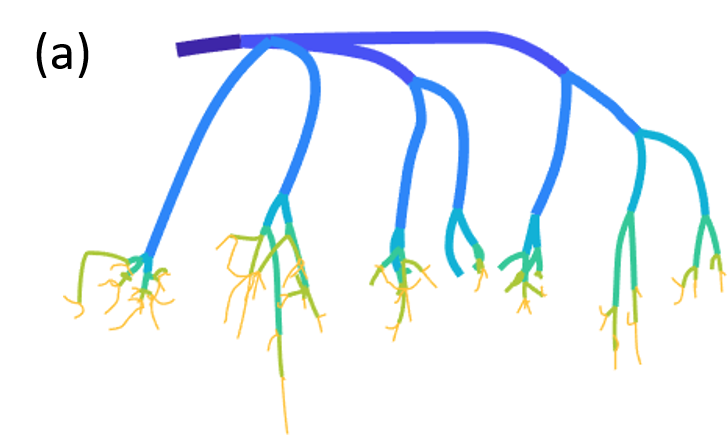
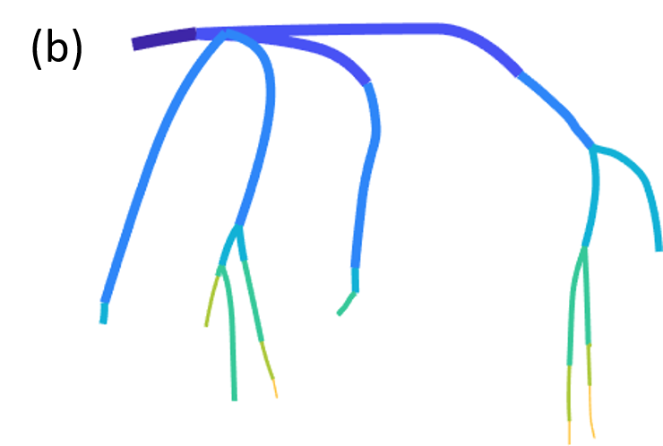
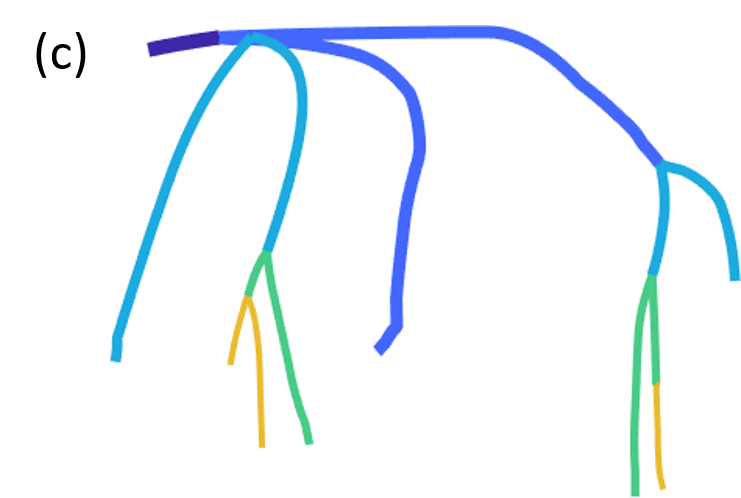
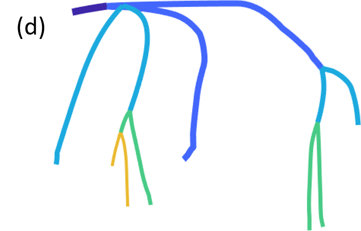
Figure 6: The evolution of a tree as it passes through some of the filters discussed here; line weight and colour indicate generation affiliation; the Mercator projection preserves the tree structure but not segment length. (a) Generations 0 – 5 of the tree without pseudo-trifurcations. (b) Segments from a that additionally have mean radius of at least 0.6 mm. (c) The segments from b have been joined in series. (d) Short terminal segments from c have been removed and the series join has been repeated.

2.5.3 Series Joins

As can be seen in Fig. 6(b), there appear to be segments that give rise to exactly one other vessel. As mentioned, much of the computational time spent during flow simulations with these networks is spent on matching the boundaries between vessels, hence it is computationally advantageous to join a parent segment and its single child to form one longer segment. Such a join is advantageous as it reduces the complexity of the tree structure without loss of information.

Figure 6(c) the tree from Fig. 6(b) in which series joins have been made. After the appropriate series joins are made, the tree contains 16 segments.

2.5.4 Additional Removal of Short segments

In Fig. 6(c) there is an instance in which a long segment appears to give rise to exactly one other vessel – it can be seen in the lower right of the panel. However, this cannot be the case as these were previously removed. Upon closer inspection of the tree, we see that these are bifurcations in which one branch is much shorter than the parent or sibling branches. The short segment here contains three nodes while its sibling contains 21. Once the short segment has been removed, eligible segments can be joined in series. Doing so with this tree reduces the number of segments to 14 organised into 5 generations. The final tree is shown in Fig. 6(d).

Currently, there is no clear optimal criteria for the additional removal of short segments from a tree. Further work is needed to set such a condition. At present, a segment is removed if it contains fewer than 5 nodes and gives rise to no further segments.

3 Conclusions and Discussion

The current analysis aims to elucidate the methods by which one research group generates connected networks of blood vessels from a single data set. This data set is from a single pig and captures a partial left coronary arterial tree. This analysis has not been applied to other, similar data sets, although we are looking into opportunities to do this in the near future. None of the algorithms used here have been optimised. There are likely to be better methods and metrics for accomplishing what we have made. However, we have created a suite of MATLAB functions that systematically reduce the scope of the coronary arterial tree to the point that they are usable in 1D flow simulations such as those discussed by Mackenzie (2021).

The main goal of the analysis discussed here was to generate various trees for 1D flow studies and to fully automate their creation.

More work needs to be done to quantify the differences between trees generated using various parameter combinations with the methods described above. Further, the definition of short segment needs to be carefully considered to ensure that segments that are not artifacts are not removed erroneously.

References

- Chambers et al. [2020] M. J. Chambers, M. J. Colebank, M. U. Qureshi, R. Clipp, and M. S. Olufsen. Structural and hemodynamic properties of murine pulmonary arterial networks under hypoxia-induced pulmonary hypertension. Proceedings of the Institution of Mechanical Engineers, Part H: Journal of Engineering in Medicine, 234(11):1312–1329, 2020.
- Nordsletten et al. [2006] D. A. Nordsletten, S. Blackett, M. D. Bentley, E. L. Ritman, and N. P. Smith. Structural morphology of renal vasculature. American Journal of Physiology-Heart and Circulatory Physiology, 291(1):H296–H309, 2006.
- van Bavel and Spaan [1992] E. van Bavel and J. A. Spaan. Branching patterns in the porcine coronary arterial tree. estimation of flow heterogeneity. Circulation research, 71(5):1200–1212, 1992.
- Hyde et al. [2014] E. R. Hyde et al. Multi-scale parameterisation of a myocardial perfusion model using whole-organ arterial networks. Annals of biomedical engineering, 42(4):797–811, 2014.
- Müller and Toro [2014] L. O. Müller and E. F. Toro. A global multiscale mathematical model for the human circulation with emphasis on the venous system. International journal for numerical methods in biomedical engineering, 30(7):681–725, 2014.
- Mynard et al. [2014] J. P. Mynard, D. J. Penny, and J. J. Smolich. Scalability and in vivo validation of a multiscale numerical model of the left coronary circulation. American Journal of Physiology-Heart and Circulatory Physiology, 306(4):H517–H528, 2014.
- Mynard and Smolich [2016] J. P. Mynard and J. J. Smolich. Influence of anatomical dominance and hypertension on coronary conduit arterial and microcirculatory flow patterns: a multiscale modeling study. American Journal of Physiology-Heart and Circulatory Physiology, 311(1):H11–H23, 2016.
- Qureshi et al. [2014] M. U. Qureshi, G. D. A. Vaughan, C. Sainsbury, M. Johnson, C. S. Peskin, M. S. Olufsen, and N. A. Hill. Numerical simulation of blood flow and pressure drop in the pulmonary arterial and venous circulation. Biomechanics and modeling in mechanobiology, 13(5):1137–1154, 2014.
- Olufsen et al. [2012] M. S. Olufsen, N. A. Hill, G. D. A. Vaughan, C. Sainsbury, and M. Johnson. Rarefaction and blood pressure in systemic and pulmonary arteries. Journal of fluid mechanics, 705:280–305, 2012.
- Lelovas et al. [2014] P. P. Lelovas, N. G. Kostomitsopoulos, and T. T. Xanthos. A comparative anatomic and physiologic overview of the porcine heart. Journal of the American Association for Laboratory Animal Science, 53(5):432–438, 2014.
- Ogden [1970] J. A. Ogden. Congenital anomalies of the coronary arteries. The American journal of cardiology, 25(4):474–479, 1970.
- Yildiz et al. [2010] A. Yildiz et al. Prevalence of coronary artery anomalies in 12,457 adult patients who underwent coronary angiography. Clinical cardiology, 33(12):E60–E64, 2010.
- Yamanaka and Hobbs [1990] O. Yamanaka and R. E. Hobbs. Coronary artery anomalies in 126,595 patients undergoing coronary arteriography. Catheterization and cardiovascular diagnosis, 21(1):28–40, 1990.
- Kardos et al. [1997] A. Kardos et al. Epidemiology of congenital coronary artery anomalies: a coronary arteriography study on a central european population. Catheterization and cardiovascular diagnosis, 42(3):270–275, 1997.
- Kassab et al. [1993] G. S. Kassab, C. A. Rider, N. J. Tang, and Y. C. Fung. Morphometry of pig coronary arterial trees. American Journal of Physiology-Heart and Circulatory Physiology, 265(1):H350–H365, 1993.
- Kassab et al. [1994] G. S. Kassab, D. H. Lin, and Y. C. Fung. Morphometry of pig coronary venous system. American Journal of Physiology-Heart and Circulatory Physiology, 267(6):H2100–H2113, 1994.
- Mackenzie [2021] J. A. Mackenzie. A 1D model for the pulmonary and coronary circulation accounting for time-varying external pressure. PhD thesis, University of Glasgow, 2021.
- Goyal et al. [2012] A. Goyal et al. Model-based vasculature extraction from optical fluorescence cryomicrotome images. IEEE transactions on medical imaging, 32(1):56–72, 2012.
- Sinclair et al. [2015] M. Sinclair et al. Microsphere skimming in the porcine coronary arteries: Implications for flow quantification. Microvascular research, 100:59–70, 2015.
- van Horssen et al. [2009] P. van Horssen et al. Extraction of coronary vascular tree and myocardial perfusion data from stacks of cryomicrotome images. In International Conference on Functional Imaging and Modeling of the Heart, pages 486–494. Springer, 2009.
- van den Wijngaard et al. [2011] J. P. H. M. van den Wijngaard et al. Porcine coronary collateral formation in the absence of a pressure gradient remote of the ischemic border zone. American Journal of Physiology-Heart and Circulatory Physiology, 300(5):H1930–H1937, 2011.
- Miller [1942] O. M. Miller. Notes on cylindrical world map projections. Geographical Review, 32(3):424–430, 1942.
- Dijkstra [1959] E. W. Dijkstra. A note on two problems in connexion with graphs. Numerische mathematik, 1(1):269–271, 1959.
- Horton [1945] R. E. Horton. Erosional development of streams and their drainage basins; hydrophysical approach to quantitative morphology. Geological society of America bulletin, 56(3):275–370, 1945.
- Strahler [1952] A. N. Strahler. Hypsometric (area-altitude) analysis of erosional topography. Geological society of America bulletin, 63(11):1117–1142, 1952.
- Strahler [1957] A. N. Strahler. Quantitative analysis of watershed geomorphology. Eos, Transactions American Geophysical Union, 38(6):913–920, 1957.
- Jiang et al. [1994] Z. L. Jiang, G. S. Kassab, and Y. C. Fung. Diameter-defined strahler system and connectivity matrix of the pulmonary arterial tree. Journal of Applied Physiology, 76(2):882–892, 1994.
- Schwen and Preusser [2012] L. O. Schwen and T. Preusser. Analysis and algorithmic generation of hepatic vascular systems. International journal of hepatology, 2012, 2012.