Stability and reconstruction of a special type of anisotropic conductivity in magneto-acoustic tomography with magnetic induction

Abstract

We consider the issues of stability and reconstruction of the electrical anisotropic conductivity of biological tissues in a domain $\Omega\subset\mathbb{R}^{3}$ by means of the hybrid inverse problem of magneto-acoustic tomography with magnetic induction (MAT-MI). The class of anisotropic conductivities considered here is of type $\sigma(\cdot)=A(\cdot,\gamma(\cdot))$ in $\Omega$, where $[\lambda^{-1},\lambda]\ni t\mapsto A(\cdot,t)$ is a one-parameter family of matrix-valued functions which are a-priori known to be $C^{1,\beta}$, allowing us to stably reconstruct $\gamma$ in $\Omega$ in terms of an internal functional $F(\sigma)$. Our results also extend previous results in MAT-MI where $\sigma(\cdot)=\gamma(\cdot)D(\cdot)$, with $D$ an a-priori known matrix-valued function on $\Omega$ to a more general anisotropic structure which depends non-linearly on the scalar function $\gamma$ to be reconstructed.

1 Introduction

In many physical situations, it is important to determine certain physical properties of the interior of a body that cannot be measured directly. Inverse problems are employed to infer such information from external observations. If one is interested in imaging biological tissue inside the human body, its electrical conductivity distribution can provide valuable information about its state. A recently developed non-invasive imaging modality based on the determination of the electrical conductivity distribution of biological tissue is Magnetoacoustic Tomography with Magnetic Induction (MAT-MI).

If a biological conductive body, modelled by a domain $\Omega\subset\mathbb{R}^{3}$ with smooth boundary $\partial\Omega$, is placed in a static magnetic field $B_{0}=(0,0,1)$, it starts to emit ultrasound waves that can be measured around the body, i.e. at a series of locations on $\partial\Omega$. To be more precise, to cause an eddy current within the conductive tissue, a pulsed time-dependent magnetic field $B(t)$ is applied to excite the tissue in $\Omega$, which, in turn, emits the ultrasound waves. For the sake of simplicity and to follow the research line already initiated in [8], [36], we assume here that $B(t)$ is time-independent and that $B(t)=B_{0}$. MAT-MI is an example of hybrid inverse problems, which typically combine a high contrast modality with a high resolution one and they typically involve two steps. In the first step, a well-posed problem involving high resolution and low contrast modality is solved from the knowledge of boundary measurements. In the second step, a quantitative reconstruction of the parameters of interest (describing a physical property of the medium in question) is solved by knowledge of a so-called internal functional which has been reconstructed during the first step. Hybrid methods are mainly concerned with the solution of the second step (assuming that the first step has been successfully performed). For a review on hybrid imaging modalities we refer to [11].

The first step in MAT-MI is to retrieve the acoustic source from the measurements around the object in the scalar wave equation. Then, in the second step, MAT-MI reconstructs the distribution of electrical conductivity from acoustic source information (see [8], [36]). This second step is the focus of this paper, where we study, in the MAT-MI experiment, the issues of stability and reconstruction for a special type of anisotropic conductivity $\sigma$ in terms of internal measurements of the acoustic sources (which are assumed to be known after the first step has been performed) modelled by the internal functional

(1.1) $$F(\sigma)=\nabla\cdot(\sigma E_{\sigma}\times B_{0}),\qquad\textnormal{in}\quad\Omega,$$

where $E_{\sigma}$ solves the Maxwell’s equations

(1.2) $$\Bigg{\{}\begin{array}[]{llll}\nabla\times E_{\sigma}&=B_{0},&\text{in}\quad\Omega,\\ \nabla\cdot\sigma E_{\sigma}&=0,&\text{on}\quad\Omega,\\ \sigma E_{\sigma}\cdot\nu&=0,&\text{on}\quad\partial\Omega\end{array}$$

and $\sigma\in C^{1,\beta}(\overline{\Omega})$ is symmetric on $\Omega$ and satisfies a uniform ellipticity condition (the precise formulation of the problem is given in section 2).

For clinical and research purposes, the electrical conductivity of biological tissues can provide valuable information as the conductivity varies significantly within the human body. Other and more established medical imaging modalities, like Computerized Tomography (CT), Magnetic Resonance Imaging (MRI) and ultrasound imaging, are typically capable of creating images of the human body with very high resolution. These modalities often fail to exhibit a sufficient contrast between different type of tissues. Imaging modalities like Optical Tomography (OT) and Electrical Impedance Tomography (EIT) do, on the other hand, display such high contrast at the expense of a poor resolution ([9], [13], [41]). EIT, similarly to MAT-MI, also provides information about materials and biological tissues in terms of their conductivity. The resulting images from measurements of electrostatic voltages and current flux taken on the surface of the body under investigation, are often blurred, due to the EIT poor resolution. MAT-MI, on the other hand, has the potential to overcome this issue by providing images of the conductivity of a body in terms of internal measurements that have been obtained by means of a high resolution imaging modality performed in the first step of MAT-MI. Hence MAT-MI has the potential to provide high contrast images of a body in terms of its internal conductivity that also benefits from a reasonably good resolution.

Biological tissues are known to have a have anisotropic conductivity [30]. In EIT, since its first mathematical formulation by A. Calderón in his 1980 seminal paper [16], a lot of progress has been made, but the problem of uniquely determining the anisotropic conductivity of a body by means of EIT measurements is still considered an open problem. Partial results of uniqueness and stability for this inverse problem have been obtained in [1], [2], [3], [4], [5], [6], [10], [12], [18], [19], [20] [21], [27], [32], [33], [34], [35], [39].

In the MAT-MI experiment, results of stability and reconstruction of the conductivity $\sigma$ in terms of the internal functional $F(\sigma)$ given in (1.1), have been obtained in [36] and [8], where the isotropic case $\sigma=\gamma I$ (here $I$ denotes the $3\times 3$ identity matrix and $\gamma$ is a positive scalar function on $\Omega$) and the special anisotropic case $\sigma=\gamma D$, with $D$ a known $3\times 3$ symmetric matrix and $\gamma$ is a positive scalar function on $\Omega$, were considered, respectively. In the present paper, we extend these results to the case where the anisotropic conductivity $\sigma$ is of type $\sigma=A(\cdot,\gamma(\cdot))$, and $A(\cdot,t)$ is known for $t\in[\lambda^{-1},\lambda]$.

More precisely, we start by considering the simpler case where $\sigma$ is a symmetric, uniformly positive definite matrix which is a-priori known to have the structure $\sigma(x)=A(\gamma(x))$, $x\in\overline{\Omega}$, where the one-parameter family of matrix-valued functions

$$t\mapsto A(t),\qquad t\in[\lambda^{-1},\lambda]$$

is assumed to be known and to belong to a certain class $\mathcal{A}$ defined below (Definition 2.2) and $\gamma=\gamma(x)$, $x\in\overline{\Omega}$ is an unknown scalar function to be determined. The above structure for $\sigma$ is also generalized to the case $\sigma=A(x,\gamma(x))$, $x\in\overline{\Omega}$, where the one-parameter family of matrix-valued functions

$$t\mapsto A(x,\>t),\qquad\textnormal{for\>any}\quad x\in\overline{\Omega},\qquad t\in[\lambda^{-1},\lambda]$$

is assumed to be known and to belong to a certain class $\mathcal{A^{\prime}}$ defined below (Definition 2.3) and $\gamma=\gamma(x)$, $x\in\overline{\Omega}$ is again an unknown scalar function to be determined. The latter, in particular, extends the results in [36] and [8], where the problem of stability and reconstruction in MAT-MI has been addressed in the isotropic case and in the anisotropic case $\sigma(x)=\gamma(x)D(x)$, where $D$, in this case, is a known matrix-valued function and $\gamma=\gamma(x)$, $x\in\overline{\Omega}$ is the unknown scalar function to be determined. For both the cases when $A\in\mathcal{A}$ and $A\in\mathcal{A^{\prime}}$ considered in this manuscript, we prove that we can stably reconstruct the scalar function $\gamma$ in terms of $F$.

In this paper we also present several numerical experiments in which we reconstruct the scalar function $\gamma=\gamma(x)$, $x\in\Omega$ for both types of anisotropic conductivities $\sigma(x)=A(\gamma(x))$ and $\sigma(x)=A(x,\gamma(x))$, $x\in\Omega$. We start by considering a number of examples in which $A\in\mathcal{A}$ only (Examples 1 - 4). The more general case of $A\in\mathcal{A^{\prime}}$ is exploited in Examples 5 and 6. The reconstruction is based on an algorithm introduced in [36], [8], which relies on projecting its iterates into a convex subset of $C^{1,\beta}(\Omega)$ in order to restore well-posedness in the inverse problem. We note that in the particular examples considered here, the projection step seems unnecessary for the convergence of the iterates. Moreover, in two of our examples, the true conductivity $\gamma_{*}$ we wish to reconstruct is not $C^{1}$, hence is less regular than the classes of conductivities we considered in our theoretical framework. This not only allows us to test the performance of the reconstruction algorithm on non-smooth data, but it also provides insights about possibly lowering the regularity of the conductivity considered in our theoretical framework (the stability estimates in 2 and the convergence analysis we carry out in 4.2). It will be part of future work to extend our theoretical framework to a class of conductivities with lower regularity assumptions and a more general anisotropic structure. The anisotropic structures considered in the current paper are one-parameter families of symmetric and uniformly positive definite matrices that depend on the unknown scalar function $\gamma$ in a nonlinear way, extending the results in [8] to the case of a more realistic dependence of the anisotropic structure on the unknown scalar function $\gamma$. We wish to stress that this paper aims at providing a first step in the treatment in MAT-MI of anisotropic structures that depend nonlinearly on (possibly) a finite number of unknown scalar functions to be stably reconstructed in the MAT-MI experiment. It will be the subject of future work to consider the fully anisotropic case and to which extent the MAT-MI experiment can be employed to determine the anisotropic structure itself.

The paper is organized as follows. In Section 2 we introduce notation, state our main assumptions, and define precisely the two classes $\mathcal{A}$ and $\mathcal{A}^{\prime}$ for $A$, corresponding to both the simpler and spatially dependent anisotropic case, respectively. The main stability results are also contained in this section. Section 3 contains the proofs of our main stability results, and includes estimates for the electromagnetic boundary value problem. In Section 4 we describe the reconstruction algorithm (Section 4.1) and prove convergence results (Section 4.2), again corresponding to both classes of $A$. Section 5 contains several numerical experiments demonstrating accurate reconstructions, including two cases of non-smooth true scalar functions $\gamma_{*}$ and one fully three dimensional reconstruction. Some final concluding remarks are included in Section 6.

2 Main assumptions and stability estimates

Throughout this paper the medium to be imaged is a bounded domain $\Omega$ in $\mathbb{R}^{3}$ with $C^{1,\beta}$ boundary $\partial\Omega$ (see definition 2.1) and diameter $\textnormal{diam}(\Omega)=M$, for some constant $M>0$. For a point $x\in\mathbb{R}^{3}$, we will denote $x=(x^{\prime},x_{3})$, where $x^{\prime}\in\mathbb{R}^{2}$ and $x_{3}\in\mathbb{R}$. We will also denote by $B_{r}$, $B^{\prime}_{r}$ the open balls $B_{r}(0)$ and $B^{\prime}_{r}(0)$ in $\mathbb{R}^{3}$ and $\mathbb{R}^{2}$, respectively and by $Q_{r}$ the cylinder $Q_{r}(0)$ in $\mathbb{R}^{3}$ defined by

$$Q_{r}(0)=B^{\prime}_{r}\times(x_{3}-r,x_{3}+r).$$

From here onwards we fix a number $\beta$ satisfying $0<\beta\leq 1$.

Definition 2.1.

Given a bounded domain $\Omega\subset\mathbb{R}^{3}$, we say that $\partial\Omega$ is of class $C^{1,\beta}$ with constants $r_{0},L>0$, if for every $P\in\partial\Omega$, there exists a rigid transformation of coordinates under which $P=0$ and

$$\Omega\cap Q_{r_{0}}=\left\{(x^{\prime},x_{n})\in Q_{r_{0}}\quad|\quad x_{3}>\varphi(x^{\prime})\right\},$$

where $\varphi$ is a $C^{1,\beta}$ function on $B^{\prime}_{r_{0}}$ satisfying

$$\varphi(0)=|\nabla\varphi(0)|=0$$

and

$$||\varphi||_{C^{1,\beta}(B^{\prime}_{r_{0}})}\leq Lr_{0},$$

where we use the normalization convention

$$||\varphi||_{C^{1,\beta}(B^{\prime}_{r_{0}})}=||\varphi||_{L^{\infty}(B^{\prime}_{r_{0}})}+r_{0}||\nabla\varphi||_{L^{\infty}(B^{\prime}_{r_{0}})}+r_{0}^{1+\beta}\sup_{x^{\prime},y^{\prime}\in B^{\prime}_{r_{0}},\>x^{\prime}\neq y^{\prime}}\frac{|\nabla\varphi(x^{\prime})-\nabla\varphi(y^{\prime})|}{|x^{\prime}-y^{\prime}|^{\beta}}.$$

Once for all it is understood that $\Omega\subset\mathbb{R}^{3}$ is a bounded domain with diameter $\textnormal{diam}(\Omega)=M$ and $C^{1,\beta}$ boundary $\partial\Omega$. We define below the two classes of admissible anisotropic structures considered in this paper.

Definition 2.2.

Given $\Lambda$, $\mathcal{E}_{1}>0$ and denoting by $Sym$ the class of $3\times 3$ real-valued symmetric matrices, we say that $A(\cdot)\in\mathcal{A}$ if the following conditions hold:

(2.1) $$A\in C^{1,\beta}([\lambda^{-1},\lambda],Sym),$$

(2.2) $$\begin{split}&\underset{t\in[\lambda^{-1},\lambda]}{\sup}\Big{|}\frac{dA}{dt}(t)\Big{|}+\underset{t_{1}\neq t_{2}}{\underset{t_{1},\>t_{2}\in[\lambda^{-1},\lambda]}{\sup}}\frac{|\frac{dA}{dt_{i}}(t_{1})-\frac{dA}{dt_{i}}(t_{2})|}{|t_{1}-t_{2}|^{\beta}}\leq\mathcal{E}_{1}\end{split}$$

and

(2.3) $$\Lambda^{-1}|\xi|^{2}\leq A(t)\xi\cdot\xi\leq\Lambda|\xi|^{2},\quad\textnormal{for\>every}\quad t\in[\lambda^{-1},\lambda],\quad\xi\in\mathbb{R}^{3}.$$

Proposition 2.1.

If $A\in\mathcal{A}$ and $\gamma$ satisfies

(2.4) $$\lambda^{-1}\leq\gamma(x) \leq \lambda,\quad\textnormal{for\>almost\>every}\>x\in\Omega,$$

(2.5) $$||\gamma||_{C^{1,\beta}(\bar{\Omega})} \leq K,$$

for some constants $\lambda,K>0$, then we have

(2.6) $$A(\gamma(\cdot))\in C^{1,\beta}(\bar{\Omega},Sym_{n})$$

and furthermore,

(2.7) $$||A(\gamma(\cdot))||_{C^{1,\beta}(\bar{\Omega})}\leq\Lambda+K\mathcal{E}_{1}M(1+2M^{\beta}):=\mathcal{F}_{1},$$

where $M$, $\mathcal{E}_{1}$ and $\Lambda$ have been introduced above.

Proof.

The proof is a straightforward consequence of equality

(2.8) $$\begin{split}||A(\gamma(\cdot))||_{C^{1,\beta}(\bar{\Omega})}&=||A(\gamma(\cdot))||_{L^{\infty}(\bar{\Omega})}\\ &+M\underset{1\leq i\leq n}{\sup}\Big{|}\Big{|}\frac{\partial A}{\partial x_{i}}(\gamma(\cdot))\Big{|}\Big{|}_{L^{\infty}(\bar{\Omega})}\\ &+M^{1+\beta}\underset{1\leq i\leq n}{\sup}\quad\underset{x\neq y}{\underset{x,y\in\bar{\Omega}}{\sup}}\frac{|\frac{\partial A}{\partial x_{i}}(\gamma(x))-\frac{\partial A}{\partial x_{i}}(\gamma(y))|}{|x-y|^{\beta}}\end{split}$$

and our assumptions. ∎

Definition 2.3.

Given $\Lambda$, $\mathcal{E}_{2}>0$, we say that $A(\cdot,\cdot)\in\mathcal{A^{\prime}}$ if the following conditions hold:

(2.9) $$A\in C^{1,\beta}(\bar{\Omega}\times[\lambda^{-1},\lambda],Sym),$$

(2.10) $$\begin{split}&\underset{t\in[\lambda^{-1},\lambda]}{\sup}\Bigg{\{}\quad\underset{1\leq i\leq n}{\sup}\Big{|}\Big{|}\frac{\partial A}{\partial x_{i}}(\cdot,t)\Big{|}\Big{|}_{L^{\infty}(\bar{\Omega})}+\Big{|}\Big{|}\frac{\partial A}{\partial t}(\cdot,t)\Big{|}\Big{|}_{L^{\infty}(\bar{\Omega})}\\ &+\underset{1\leq i\leq n}{\sup}\quad\underset{x\neq y}{\underset{x,y\in\bar{\Omega}}{\sup}}\frac{|\frac{\partial A}{\partial x_{i}}(x,t)-\frac{\partial A}{\partial x_{i}}(y,t)|}{|x-y|^{\beta}}+\underset{x\neq y}{\underset{x,y\in\bar{\Omega}}{\sup}}\frac{|\frac{\partial A}{\partial t}(x,t)-\frac{\partial A}{\partial t}(y,t)|}{|x-y|^{\beta}}\Bigg{\}}\\ &+\underset{t_{1}\neq t_{2}}{\underset{t_{1},\>t_{2}\in[\lambda^{-1},\lambda]}{\sup}}\Bigg{\{}\frac{||\frac{\partial A}{\partial x_{i}}(\cdot,t_{1})-\frac{\partial A}{\partial x_{i}}(\cdot,t_{2})||_{L^{\infty}(\bar{\Omega})}}{|t_{1}-t_{2}|^{\beta}}+\frac{||\frac{\partial A}{\partial t}(\cdot,t_{1})-\frac{\partial A}{\partial t}(\cdot,t_{2})||_{L^{\infty}(\bar{\Omega})}}{|t_{1}-t_{2}|^{\beta}}\Bigg{\}}\leq\mathcal{E}_{2}\end{split}$$

and

(2.11) $$\Lambda^{-1}|\xi|^{2}\leq A(x,t)\xi\cdot\xi\leq\Lambda|\xi|^{2},\quad\textnormal{for\>a.e.}\>x\in\bar{\Omega},\quad\forall t\in[\lambda^{-1},\lambda],\quad\forall\xi\in\mathbb{R}^{3}.$$

We observe that (2.3), (2.11) are conditions of uniform ellipticity.

Proposition 2.2.

If $A\in\mathcal{A^{\prime}}$ and $\gamma$ satisfies (2.4), (2.5), then we have

(2.12) $$||A(\cdot,\gamma(\cdot))||_{C^{1,\beta}(\bar{\Omega})}\leq\Lambda+M\mathcal{E}_{2}(1+K)(1+2M^{\beta}):=\mathcal{F}_{2},$$

where where $M$, $\mathcal{E}_{2}$ and $\Lambda$ have been introduced above.

Proof.

This is a straightforward consequence of equalities

(2.13) $$\frac{\partial A}{\partial x_{i}}(x,\gamma(x))=\frac{\partial A}{\partial x_{i}}(x,t)\big{|}_{(x,t)=(x,\gamma(x))}+\frac{\partial A}{\partial t}(x,t)\big{|}_{(x,t)=(x,\gamma(x))}\frac{\partial\gamma}{\partial x_{i}}(x),$$

together with our assumptions. ∎

Below are our two stability estimates of $\gamma$ in terms of the internal functional $F$ for the two classes of admissible anisotropic structures $\mathcal{A}$ and $\mathcal{A^{\prime}}$, respectively.

Theorem 2.3.

Let $A\in\mathcal{A}$ and assume $\gamma_{i}$ satisfies (2.4), (2.5), for $i=1,2$, $\gamma_{1}=\gamma_{2}$ on $\partial\Omega$ and

(2.14) $$||\nabla(\gamma_{1}-\gamma_{2})||_{L^{2}(\Omega)} \leq\mathcal{C}||\gamma_{1}-\gamma_{2}||_{L^{2}(\Omega)},$$

for some constant $\mathcal{C}>0$. Denoting

(2.15) $$F_{i}:=\nabla\cdot(A(\gamma_{i})E_{A(\gamma_{i})}\times B_{0}),\qquad\textnormal{for}\quad i=1,2,$$

if $\mathcal{C}\Big{(}C_{1}(\mathcal{E}_{1}+1)+\Lambda C_{3}\Big{)}<\frac{1}{2}$, where $C_{1}=(1+\Lambda\mathcal{F}_{1})(\frac{1}{2}M(\mu(\Omega))^{\frac{1}{2}})$ and $C_{3}=\Lambda\mathcal{E}_{1}C_{1}$, then

(2.16) $$||\gamma_{1}-\gamma_{2}||_{L^{2}(\Omega)}\leq C||F_{1}-F_{2}||_{L^{2}(\Omega)},$$

where $C>0$ is a constant that depends on $\mathcal{C}$, $K$, $\mathcal{E}_{1}$, $\Lambda$, $M$, $r_{0}$ and $L$ only.

More generally, we obtain the following main stability result.

Theorem 2.4.

Let $A\in\mathcal{A}^{\prime}$ and $\gamma_{i}$ be as in Theorem 2.3, for $i=1,2$. Denoting

(2.17) $$\tilde{F}_{i}:=\nabla\cdot(A(\cdot,\>\gamma_{i})E_{A(\cdot,\>\gamma_{i})}\times B_{0}),\qquad\textnormal{for}\quad i=1,2,$$

if $\mathcal{C}\Big{(}C_{2}(\mathcal{E}_{2}+1)+\Lambda C_{4}\Big{)}<\frac{1}{2}$, where $C_{2}=(1+\Lambda\mathcal{F}_{2})(\frac{1}{2}M(\mu(\Omega))^{\frac{1}{2}})$ and $C_{4}=\Lambda\mathcal{E}_{2}C_{2}$, then

(2.18) $$||\gamma_{1}-\gamma_{2}||_{L^{2}(\Omega)}\leq\tilde{C}||\tilde{F}_{1}-\tilde{F}_{2}||_{L^{2}(\Omega)},$$

where $\tilde{C}>0$ is a constant that depends on $\mathcal{C}$, $K$, $\mathcal{E}_{2}$, $\Lambda$, $M$, $r_{0}$ and $L$ only.

3 Proof of the stability estimates

To prove our main stability results, we proceed by reducing the Maxwell system (1.2) into a Neumann boundary value problem, for which we recall standard estimates that will be needed for the arguments in the proofs of our stability results.

3.1 Technical results

In what follows we recall standard estimates for the solution of Neumann boundary value problems of type

(3.1) $$\Bigg{\{}\begin{array}[]{llll}\nabla\cdot(\sigma\nabla u)&=-\nabla\cdot E,&\text{in}\quad\Omega,\\ (\sigma\nabla u+E)\cdot\nu&=0,&\text{on}\quad\partial\Omega.\end{array}$$

Such estimates are standard in the theory of elliptic partial differential equations and we recall them, together with their proof, for the sake of completeness.

Proposition 3.1.

Let $\sigma\in C^{1,\beta}(\overline{\Omega})$ be a matrix-valued function satisfying the uniform ellipticity condition

(3.2) $$\Lambda^{-1}|\xi|^{2}\leq\sigma(x)\xi\cdot\xi\leq\Lambda|\xi|^{2},\quad\textnormal{for\>a.e.}\>x\in\bar{\Omega},\quad\forall\xi\in\mathbb{R}^{3}$$

and let $E\in$ $L^{2}(\Omega)$ be a vector-valued function. The Neumann problem (3.1) has a unique solution $u\in H^{1}(\Omega)$ (up to an additive constant) that satisfies

(3.3) $$||\nabla u||_{L^{2}(\Omega)}\leq\Lambda||E||_{L^{2}(\Omega)}.$$

Proof.

As a straighforward consequence of

(3.4) $$\int_{\Omega}A\nabla{u}\cdot\nabla u\>dx=-\int_{\Omega}{E}\cdot\nabla{u}\>dx,$$

we obtain

(3.5) $$\Lambda^{-1}||\nabla{u}||^{2}_{L^{2}(\Omega)}\leq\Big{|}-\int_{\Omega}{E}\cdot\nabla{u}dx\Big{|}\leq||{E}||_{L^{2}(\Omega)}||\nabla{u}||_{L^{2}(\Omega)},$$

which concludes the proof. ∎

Proposition 3.2.

Let $\gamma_{i}$ satisfy (2.4), (2.5), for $i=1,2$.

1. If $A\in\mathcal{A}$ and $\sigma_{i}(x)=A(\gamma_{i}(x))$, $x\in\overline{\Omega}$, for $i=1,2$, then we have

   (3.6) $$||E_{A(\gamma_{i})}||_{C^{1,\beta}(\Omega)}\leq C_{1},\qquad\textnormal{for}\>i=1,2,$$

   (3.7) $$||E_{A(\gamma_{1})}-E_{A(\gamma_{2})}||_{L^{2}(\Omega)}\leq C_{3}||\gamma_{1}-\gamma_{2}||_{L^{2}(\Omega)},$$

   (3.8) $$||E_{A(\gamma_{1})}-E_{A(\gamma_{2})}||_{H^{1}(\Omega)}\leq\tilde{C_{3}}||\gamma_{1}-\gamma_{2}||_{H^{1}(\Omega)},$$

   where $E_{A(\gamma_{i})}$ is the unique solution to (1.2), with $\sigma_{i}=A(\gamma_{i})$, for $i=1,2$ and $C_{1}$, $C_{3}$, $\tilde{C_{3}}$ are positive constants depending only on $\Lambda$, $r_{0}$ and $L$.

2. Similarly, if and $A\in\mathcal{A}^{\prime}$ and $\sigma_{i}(x)=A(x,\gamma_{i}(x))$, $x\in\overline{\Omega}$, for $i=1,2$, then we have

   (3.9) $$||E_{A(\cdot,\gamma_{i})}||_{C^{1,\beta}(\Omega)}\leq C_{2},\qquad\textnormal{for}\>i=1,2,$$

   (3.10) $$||E_{A(\cdot,\gamma_{1})}-E_{A(\cdot,\gamma_{2})}||_{L^{2}(\Omega)}\leq C_{4}||\gamma_{1}-\gamma_{2}||_{L^{2}(\Omega)},$$

   (3.11) $$||E_{A(\cdot,\gamma_{1})}-E_{A(\cdot,\gamma_{2})}||_{H^{1}(\Omega)}\leq\tilde{C_{4}}||\gamma_{1}-\gamma_{2}||_{H^{1}(\Omega)},$$

   where $E_{A(\cdot,\gamma_{i})}$ is the unique solution to (1.2), with $\sigma_{i}=A(\cdot,\gamma_{i})$, for $i=1,2$, with $C_{2}$, $C_{4}$, $\tilde{C_{4}}$ being positive constants depending only on $\Lambda$, $r_{0}$ and $L$.

Proof.

As the proof follows the same line of [8, Proof of Proposition 2], we only highlight the main steps of case $(a)$ and only point out where case $(b)$ differs from it, as such modifications are minor. For case $(a)$ we start by noticing that for $\tilde{E}$ = $\frac{1}{2}(-y,x,0)$ we have that $\nabla\times(E_{A(\gamma_{i})}-\tilde{E})=0$, for $i=1,2$ and $E_{A(\gamma_{i})}=\tilde{E}+\nabla u$, where $u_{i}$ solves the Neumann problem

(3.12) $$\Bigg{\{}\begin{array}[]{llll}\nabla\cdot(A(\gamma_{i})\nabla u_{i})&=-\nabla\cdot(A(\gamma_{i})\tilde{E})&\textnormal{in}\quad\Omega;\\ (A(\gamma_{i})\nabla u_{i}+A(\gamma_{i})\tilde{E})\cdot\nu&=0&\textnormal{on}\quad\partial\Omega,\end{array}$$

for $i=1,2$. Observing that

(3.13) $$||\tilde{E}||_{L^{2}(\Omega)}\leq\frac{1}{2}M\big{(}\mu(\Omega)\big{)}^{\frac{1}{2}},$$

where $\mu(\Omega)$ denotes the Lebesgue measure of $\Omega$, estimate (3.6) is a straightforward consequence of (2.5) and proposition 2.1 (see also [8]).

To prove (3.7), (3.8), we start by simplifying our notation. We denote $E_{A(\gamma_{i})}$, simply with $E_{i}$, for $i$ = 1, 2. Noting that $\nabla\times E_{1}=\nabla\times E_{2}$, we write

(3.14) $$\nabla v=E_{1}-E_{2},$$

where $v$ is the unique solution to

(3.15) $$\Bigg{\{}\begin{array}[]{llll}\nabla\cdot(A(\gamma_{1})\nabla v)&=-\nabla\cdot((A(\gamma_{1})-A(\gamma_{2}))E_{2})&\textnormal{in}\quad\Omega,\\ (A(\gamma_{1})\nabla v+(A(\gamma_{1})-A(\gamma_{2}))E_{2})\cdot\nu&=0&\textnormal{on}\quad\partial\Omega\end{array}$$

and

(3.16) $$\int_{\partial\Omega}v=0.$$

Thus by Cauchy Schwartz we obtain

(3.17) $$\int_{\Omega}A(\gamma_{1})\nabla{v}\cdot\nabla{v}dx\leq\int_{\Omega}((A(\gamma_{1})-A(\gamma_{2})){E_{2}})\cdot\nabla{v}\>dx,$$

which, combined with (3.6) and the uniform ellipticity condition (2.3), leads to

(3.18) $$||\nabla{v}||_{L^{2}(\Omega)}\leq\Lambda C_{1}||A(\gamma_{1})-A(\gamma_{2})||_{L^{2}(\Omega)}.$$

From the Lagrange Theorem, for every $x\in\Omega$, there exists $t(x)$, $0<t(x)<1$, such that

(3.19) $$A(\gamma_{1}(x))-A(\gamma_{2}(x))=(\gamma_{1}-\gamma_{2})(x)\>\frac{dA(t)}{dt}\Big{|}_{t=c(x)},$$

where $c(x)=\gamma_{2}(x)+t(x)\big{(}\gamma_{1}(x)-\gamma_{2}(x)\big{)}$. Hence we obtain

(3.20) $$||\nabla v||_{L^{2}(\Omega)}\leq\Lambda C_{1}||\gamma_{1}-\gamma_{2}||_{L^{2}(\Omega)}\Big{|}\Big{|}\frac{dA(t)}{dt}\Big{|}_{t=c(\cdot)}\Big{|}\Big{|}_{L^{2}(\Omega)}$$

and

(3.21) $$||E_{1}-E_{2}||_{L^{2}(\Omega)}\leq C_{3}||\gamma_{1}-\gamma_{2}||_{L^{2}(\Omega)},$$

where $C_{3}=\Lambda\mathcal{E}_{1}C_{1}$. From the standard theory of elliptic equations

(3.22) $$||v||_{H^{2}(\Omega)}\leq C||\nabla\cdot((A(\gamma_{1})-A(\gamma_{2}))E_{2})||_{L^{2}(\Omega)},$$

where $C$ is a positive constant depending only on $\lambda$, $\Lambda$, $r_{0}$ and $L$, which implies (3.8).

For case $(b)$, where $A\in\mathcal{A^{\prime}}$ and $\gamma_{i}\in C^{1,\beta}(\overline{\Omega})$ is a scalar function satisfying (2.4), for $i=1,2$, we have, by (3.13) and proposition 3.1 that

(3.23) $$||E_{A(\cdot,\gamma_{i})}||_{L^{2}(\Omega)}\leq C_{2},\qquad\textnormal{for}\>i=1,2,$$

where $C_{2}=(1+\Lambda\mathcal{F}_{2})(\frac{1}{2}M(\mu(\Omega))^{\frac{1}{2}})$. With a similar argument to case $(a)$, from the Lagrange Theorem, for every $x\in\Omega$, there exists $t(x)$, $0<t(x)<1$, such that

(3.24) $$A(x,\gamma_{1}(x))-A(x,\gamma_{2}(x))=(\gamma_{1}-\gamma_{2})(x)\frac{\partial A(x,\>t)}{\partial t}\Big{|}_{t=c(x)},$$

where $c(x)=\gamma_{2}(x)+t(x)\big{(}\gamma_{1}(x)-\gamma_{2}(x)\big{)}$, which leads to

(3.25) $$||E_{1}-E_{2}||_{L^{2}(\Omega)}\leq\Lambda C_{1}||\gamma_{1}-\gamma_{2}||_{L^{2}(\Omega)}\Big{|}\Big{|}\frac{\partial A(\cdot,\>t)}{\partial t}\Big{|}_{t=c(\cdot)}\Big{|}\Big{|}_{L^{2}(\Omega)},$$

hence

(3.26) $$||E_{1}-E_{2}||_{L^{2}(\Omega)}\leq C_{4}||\gamma_{1}-\gamma_{2}||_{L^{2}(\Omega)},$$

where $C_{4}=\Lambda\mathcal{E}_{2}C_{2}$. The remaining (3.11) follows by a similar argument used to prove (3.8) in case $(a)$. ∎

3.2 Proof of the stability estimates

Proof of Theorem 2.3.

We write the difference in the data $F_{1}-F_{2}$ as

(3.27) $$\begin{split}F_{1}-F_{2}&=\nabla\cdot\Big{(}A(\gamma_{1})E_{1}\times B_{0}\Big{)}-\nabla\cdot\Big{(}A(\gamma_{2})E_{2}\times B_{0}\Big{)}\\ &=\nabla\cdot\Big{(}(A(\gamma_{1})-A(\gamma_{2}))E_{1}\times B_{0}\Big{)}+\nabla\cdot\Big{(}A(\gamma_{2})(E_{1}-E_{2})\times B_{0}\Big{)}\end{split}$$

and from the Lagrange Theorem, for every $x\in\Omega$, there exists $t(x)$, $0<t(x)<1$, such that

(3.28) $$F_{1}-F_{2}=\nabla\cdot\Big{(}(\gamma_{1}-\gamma_{2})\frac{dA}{dt}(t)\Big{|}_{t=c(\cdot)}E_{1}\times B_{0}\Big{)}+\nabla\cdot\Big{(}A(\gamma_{2})\>(E_{1}-E_{2})\times B_{0}\Big{)},$$

where $c(x)=\gamma_{2}(x)+t(x)\big{(}\gamma_{1}(x)-\gamma_{2}(x)\big{)}$. Then, we can split $F_{1}-F_{2}$ into three contributions

(3.29) $$F_{1}-F_{2}=I_{1}+I_{2}+I_{3},$$

where

(3.30) $$\begin{split}&I_{1}=\nabla\cdot\Big{(}(\gamma_{1}-\gamma_{2})E_{1}\times B_{0}\Big{)},\\ &I_{2}=\nabla\cdot\Big{(}(\gamma_{1}-\gamma_{2})\Big{(}\frac{dA}{dt}(t)\Big{|}_{t=c(\cdot)}-I\Big{)}E_{1}\times B_{0}\Big{)},\\ &I_{3}=\nabla\cdot\Big{(}A(\gamma_{2})(E_{1}-E_{2})\times B_{0}\Big{)},\end{split}$$

where $I$ denotes the $3\times 3$ identity matrix. To extract information about $\gamma_{1}-\gamma_{2}$ in $\Omega$ we multiply the data difference $F_{1}-F_{2}$ by $\gamma_{1}-\gamma_{2}$ and integrate over $\Omega$. We do this by considering each contribution $I_{i}$, i = 1, 2, 3, to the data separately. Starting with $I_{1}$, we obtain

(3.31) $$\begin{split}\int_{\Omega}(\gamma_{1}-\gamma_{2})I_{1}dx&=\int_{\Omega}(\gamma_{1}-\gamma_{2})^{2}\nabla\cdot(E_{1}\times B_{0})\\ &+\frac{1}{2}\nabla(\gamma_{1}-\gamma_{2})^{2}\cdot(E_{1}\times B_{0})dx\\ &=\frac{1}{2}\int_{\Omega}(\gamma_{1}-\gamma_{2})^{2}\nabla\cdot(E_{1}\times B_{0})dx\\ &=\frac{1}{2}||\gamma_{1}-\gamma_{2}||^{2}_{L^{2}(\Omega)},\end{split}$$

where in the second equality of (3.31) we performed integration by parts and used the fact that $\gamma_{1}$ and $\gamma_{2}$ share the same boundary values. In the last equality, we used the fact that $\nabla\cdot(E_{1}\times B_{0})=1$.

Multiplying $I_{2}$ by $\gamma_{1}-\gamma_{2}$, we have

(3.32) $$\begin{split}\left|\int_{\Omega}(\gamma_{1}-\gamma_{2})I_{2}dx\right|&=\Big{|}\int_{\Omega}(\gamma_{1}-\gamma_{2})^{2}\nabla\cdot\left(\Big{(}\frac{dA}{dt}(t)\Big{|}_{t=c(\cdot)}-I\Big{)}E_{1}\times B_{0}\right)\\ &+(\gamma_{1}-\gamma_{2})\nabla(\gamma_{1}-\gamma_{2})\cdot\left(\Big{(}\frac{dA}{dt}(t)\Big{|}_{t=c(\cdot)}-I\Big{)}E_{1}\times B_{0}\right)dx\Big{|}\\ &=\Big{|}\int_{\Omega}(\gamma_{1}-\gamma_{2})\nabla(\gamma_{1}-\gamma_{2})\cdot\left(\Big{(}\frac{dA}{dt}(t)\Big{|}_{t=c(\cdot)}-I\Big{)}E_{1}\times B_{0}\right)dx\Big{|}\\ &\leq\mathcal{C}C_{1}|\mathcal{E}_{1}-1|||\gamma_{1}-\gamma_{2}||^{2}_{L^{2}(\Omega)},\end{split}$$

where in the second equality of (3.32) we again performed integration by parts and again recalled that $\gamma_{1}$ and $\gamma_{2}$ share the same boundary. In the inequality, estimate (2.2), (2.14) and (3.6) have been used.

Finally, multiplyig $I_{3}$ by $\gamma_{1}-\gamma_{2}$, leads to

(3.33) $$\begin{split}\left|\int_{\Omega}(\gamma_{1}-\gamma_{2})I_{3}dx\right|&=\left|\int_{\Omega}\nabla(\gamma_{1}-\gamma_{2})\cdot\Big{(}A(\gamma_{2})(E_{1}-E_{2})\times B_{0}\Big{)}dx\right|\\ &\leq\mathcal{C}\Lambda C_{3}||\gamma_{1}-\gamma_{2}||^{2}_{L^{2}(\Omega)},\end{split}$$

where the first equality in (3.33) is derived again by performing integration by parts and noticing that $\gamma_{1}$ and $\gamma_{2}$ share the same boundary values. In the inequality, (2.3), assumption (2.14) and (3.7) have been used.

Hence, for $\mathcal{C}C_{1}(\mathcal{E}_{1}+1)+\mathcal{C}\Lambda C_{3}<\frac{1}{2}$, we obtain

(3.34) $$\int_{\Omega}(\gamma_{1}-\gamma_{2})(F_{1}-F_{2})dx\geq C||\gamma_{1}-\gamma_{2}||^{2}_{L^{2}(\Omega)},$$

where $C=\frac{1}{2}-\mathcal{C}\Big{(}C_{1}(\mathcal{E}_{1}+1)+\Lambda C_{3}\Big{)}>0$, which concludes the proof. ∎

Proof of Theorem 2.4.

Similarly to the proof of theorem 2.3, we write the data difference as

(3.35) $$\begin{split}\tilde{F}(\gamma_{1})-\tilde{F}(\gamma_{2})&=\nabla\cdot(A(\cdot,\gamma_{1})E_{1}\times B_{0})-\nabla\cdot(A(\cdot,\gamma_{2})E_{2}\times B_{0})\\ &=\nabla\cdot((A(\cdot,\gamma_{1})-A(\cdot,\gamma_{2}))E_{1}\times B_{0})+\nabla\cdot(A(\cdot,\gamma_{2})(E_{1}-E_{2})\times B_{0}).\end{split}$$

From the Lagrange Theorem, for every $x\in\Omega$, there exists $t(x)$, $0<t(x)<1$, such that

(3.36) $$A(x,\gamma_{1})-A(x,\gamma_{2})=(\gamma_{1}-\gamma_{2})(x)\frac{\partial A(x,t)}{\partial t}\Big{|}_{t=c(x)},$$

where $c(x)=\gamma_{2}(x)+t(x)\big{(}\gamma_{1}(x)-\gamma_{2}(x)\big{)}$. Therefore we obtain

(3.37) $$\tilde{F}_{1}-\tilde{F}_{2}=\nabla\cdot((\gamma_{1}-\gamma_{2})\frac{\partial A(\cdot,t)}{\partial t}\Big{|}_{t=c(x)}E_{1}\times B_{0})+\nabla\cdot(A(\cdot,\>\gamma_{2})(E_{1}-E_{2})\times B_{0}).$$

By splitting again $\tilde{F}_{1}-\tilde{F}_{2}$ as

(3.38) $$\tilde{F}_{1}-\tilde{F}_{2}=I_{1}+I_{2}+I_{3},$$

where

(3.39) $$\begin{split}&I_{1}=\nabla\cdot\Big{(}(\gamma_{1}-\gamma_{2})E_{1}\times B_{0}\Big{)},\\ &I_{2}=\nabla\cdot\left((\gamma_{1}-\gamma_{2})\Big{(}\frac{\partial A(\cdot,t)}{\partial t}\Big{|}_{t=c(\cdot)}-I\Big{)}E_{1}\times B_{0}\right),\\ &I_{3}=\nabla\cdot\Big{(}A(\cdot,\>\gamma_{2})(E_{1}-E_{2})\times B_{0}\Big{)},\end{split}$$

with a similar procedure as that of the proof of Theorem 2.3 we obtain the following estimates

(3.40) $$\begin{split}\int_{\Omega}(\gamma_{1}-\gamma_{2})I_{1}dx&=\frac{1}{2}||\gamma_{1}-\gamma_{2}||^{2}_{L^{2}(\Omega)}.\end{split}$$

(3.41) $$\begin{split}\left|\int_{\Omega}(\gamma_{1}-\gamma_{2})I_{2}dx\right|&=\left|\int_{\Omega}(\gamma_{1}-\gamma_{2})\nabla(\gamma_{1}-\gamma_{2})\cdot\left(\Big{(}\frac{\partial A(\cdot,\>t)}{\partial t}\Big{|}_{t=c(\cdot)}-I\Big{)}E_{1}\times B_{0}\right)dx\right|\\ &\leq\mathcal{C}C_{2}|\mathcal{E}_{2}-1|||\gamma_{1}-\gamma_{2}||^{2}_{L^{2}}.\end{split}$$

(3.42) $$\begin{split}\left|\int_{\Omega}(\gamma_{1}-\gamma_{2})I_{3}dx\right|&=\left|\int_{\Omega}\nabla(\gamma_{1}-\gamma_{2})\cdot(A(\cdot,\>\gamma_{2}(\cdot))\>(E_{1}-E_{2})\times B_{0})dx\right|\\ &\leq\mathcal{C}\Lambda C_{4}||\gamma_{1}-\gamma_{2}||^{2}_{L^{2}}\end{split}$$

By combining (3.40) - (3.42) together and choosing the parameters such that$(\mathcal{C}C_{2}(\mathcal{E}_{2}+1)+\mathcal{C}\Lambda C_{4})<\frac{1}{2}$, we finally obtain

(3.43) $$\int_{\Omega}(\gamma_{1}-\gamma_{2})(\tilde{F}(\gamma_{1})-\tilde{F}(\gamma_{2}))dx\geq\tilde{C}||\gamma_{1}-\gamma_{2}||^{2}_{L^{2}(\Omega)},$$

where $\tilde{C}=\frac{1}{2}-(\mathcal{C}C_{2}(\mathcal{E}_{2}+1)+\mathcal{C}\Lambda C_{4})>0$, which concludes the proof. ∎

4 Reconstruction of $\gamma$

4.1 The functional framework and the algorithm

To ensure well-posedness of the inverse problem we introduce a functional framework, similar to that in [8], based assuming that $\gamma$ is known on the boundary of $\Omega$ and by letting the true scalar function to be $\gamma_{*}$ (the unknown conductivity to be reconstructed) in $\Omega$, belonging to a bounded convex subset $\tilde{S}$ of $C^{1,\beta}(\Omega)$, defined by

(4.1) $$\tilde{S}=\{\gamma:=\gamma_{0}+\alpha|\alpha\in S\},$$

where $\gamma_{0}$ satisfies (2.4), (2.5) and

(4.2) $$S=\{\alpha\in C^{1,\beta}_{0}(\Omega)|\lambda^{-1}\leq\alpha+\gamma_{0}\leq\lambda,||\nabla\alpha||_{L^{2}(\Omega)}\leq\mathcal{C}||\alpha||_{L^{2}(\Omega)},||\alpha||_{L^{2}(\Omega)}\leq\tilde{k}\},$$

for some positive constant $\tilde{k}$.
For $A\in\mathcal{A}$, the true conductivity is denoted by $A_{*}:=A(\gamma_{*})$ and the forward operator is given by

(4.3) $$F(\gamma)=\nabla\cdot(A(\gamma)E_{A(\gamma)}\times B_{0}),$$

where $E_{A}:=E_{A(\gamma)}$ solves

(4.4) $$\Bigg{\{}\begin{array}[]{llll}\nabla\times E_{A}&=B_{0},&\text{in}\quad\Omega,\\ \nabla\cdot A(\gamma)E_{A}&=0,&\text{on}\quad\Omega,\\ A(\gamma)E_{A}\cdot\nu&=0,&\text{on}\quad\partial\Omega\end{array}$$

and the scalar function $\gamma$ is updated by solving a stationary advection-diffusion equation as shown in the algorithm below.

The Algorithm (reconstruction)

• We choose an initial conductivity $\gamma_{1}\in\tilde{S}$ and set $k=1$.

• At step $k$, defining $A_{k}:=A(\gamma_{k})$, we solve the boundary value problem

  (4.5) $$\Bigg{\{}\begin{array}[]{llll}\nabla\times E_{k}&=B_{0},&\text{in}\quad\Omega,\\ \nabla\cdot A_{k}E_{k}&=0,&\text{on}\quad\Omega,\\ A_{k}E_{k}\cdot\nu&=0,&\text{on}\quad\partial\Omega.\end{array}$$

  to update the electric field $E_{k}$.

• By solving the stationary advection-diffusion equation with the inflow boundary condition, we calculate the updated conductivity $A_{k+1/2}:=A(\gamma_{k+1})$ as follows

  (4.6) $$\Big{\{}\begin{array}[]{llll}\nabla\cdot(A_{k+1/2}E_{k}\times B_{0})&=\nabla\cdot(A_{*}E_{A_{*}}\times B_{0}),&\text{in}\quad\Omega,\\ \gamma_{k+1/2}&=\gamma_{*},&\text{on}\quad\partial\Omega^{-},\end{array}$$

  where

  (4.7) $$\partial\Omega^{-}=\left\{x\in\partial\Omega|A(\gamma_{k}(x))E_{k}(x)\times B_{0}\cdot\nu(x)<0\right\}.$$

• We then let $\gamma_{k+1}=T[\gamma_{k+1/2}]$ where $T$ is the Hilbert projection operator onto $\tilde{S}$, where the projection $T$ is needed as $\gamma_{k}$ might not be in $\tilde{S}$. Finally, we set $k=k+1$ and go to (4.5).

For $A\in\mathcal{A^{\prime}}$ the true conductivity is denoted by $A_{*}:=A(\cdot,\gamma_{*})$ and the forward operator is given by

(4.8) $$\tilde{F}(\gamma)=\nabla\cdot(A(\cdot,\gamma)E_{A(\cdot,\gamma)}\times B_{0}),$$

where $E_{A}:=E_{A(\cdot,\gamma)}$ solves

(4.9) $$\Bigg{\{}\begin{array}[]{llll}\nabla\times E_{A}&=B_{0},&\text{in}\quad\Omega,\\ \nabla\cdot A(\cdot,\gamma)E_{A}&=0,&\text{on}\quad\Omega,\\ A(\cdot,\gamma)E_{A}\cdot\nu&=0,&\text{on}\quad\partial\Omega\end{array}$$

and the scalar function $\gamma$ together with the electric field $E$ are updated as per Algorithm 1 above, where the inflow part of the boundary is in this case defined by

(4.10) $$\partial\Omega^{-}=\left\{x\in\partial\Omega|A(x,\gamma_{k}(x))E_{k}(x)\times B_{0}\cdot\nu(x)<0\right\}.$$

4.2 Convergence analysis

Under a smallness condition on $\frac{dA(t)}{dt}$ and $\frac{\partial A(\cdot,t)}{dt}$, on $[\lambda^{-1},\lambda]$ with respect to $I$, for $A\in\mathcal{A}$ and $A\in\mathcal{A^{\prime}}$, respectively (see (4.12) and (4.15), respectively), we obtain the following convergence results.

Theorem 4.1.

Suppose that the true conductivity $\gamma_{*}\in\tilde{S}$. Let $A\in\mathcal{A}$ and, additionally, assume that

(4.11) $$\frac{dA}{dt}\in C^{1}\left([\lambda^{-1},\lambda],Sym\right)$$

and that there is a constant $\tilde{\mathcal{E}}_{1}$, $0<\tilde{\mathcal{E}}_{1}<1$ such that

(4.12) $$\sup_{t\in[\lambda^{-1},\lambda]}\sup_{x\in\Omega}\left|\nabla\cdot\left[\left(\frac{dA}{dt}-I\right)E_{k}\times B_{0}\right]\right|\leq\tilde{\mathcal{E}}_{1}.$$

Assume that either

1. $$\gamma_{k}=\gamma_{*},\qquad\textnormal{on}\quad\partial\Omega,\quad\textnormal{for\>any}\>k,\quad k\geq 1;$$

   or

2. $$\gamma_{k}=\gamma_{*},\qquad\textnormal{on}\quad\partial\Omega^{-}\quad\textnormal{and}\quad\sup_{t\in[\lambda^{-1},\lambda]}\frac{dA}{dt}E_{k}\times B_{0}\cdot\nu\geq 0,\qquad\textnormal{on}\quad\partial\Omega^{+},$$

   $$\textnormal{for\>any}\>k,\quad k\geq 1.$$

Then, for an appropriate choice of $\mathcal{C}$, $\Lambda$, $C_{1}$, $\tilde{C_{3}}$, $\mathcal{E}_{1}$ and $\tilde{\mathcal{E}_{1}}$, there exists a constant $C$, $0<C<1$ such that

(4.13) $$||\gamma_{k+1}-\gamma_{*}||_{L^{2}(\Omega)}\leq C||\gamma_{k}-\gamma_{*}||_{L^{2}(\Omega)}.\\ \\$$

Theorem 4.2.

Suppose that the true conductivity $\gamma_{*}\in\tilde{S}$. Let $A\in\mathcal{A^{\prime}}$, and, additionally, assume that

(4.14) $$\frac{\partial A(\cdot,t)}{\partial t}\in C^{1}(\overline{\Omega}\times[\lambda^{-1},\lambda],Sym)$$

and there exists a constant $\tilde{\mathcal{E}_{2}}$, $0<\tilde{\mathcal{E}_{2}}<1$ such that

(4.15) $$\underset{t\in[\lambda^{-1},\lambda]}{\sup}\sup_{x\in\Omega}\quad\Big{|}\nabla\cdot\Big{[}\Big{(}\frac{\partial A}{\partial t}(\cdot,t)\Big{|}_{t=c(\cdot)}-I\Big{)}E_{k}\times B_{0}\Big{]}\Big{|}\leq\tilde{\mathcal{E}_{2}}.$$

Assume that either

1. $$\gamma_{k}=\gamma_{*},\qquad\textnormal{on}\quad\partial\Omega,\quad\textnormal{for\>any}\>k,\quad k\geq 1;$$

   or

2. $$\gamma_{k}=\gamma_{*},\qquad\textnormal{on}\quad\partial\Omega^{-}\quad\textnormal{and}\quad\sup_{t\in[\lambda^{-1},\lambda]}\frac{\partial A(\cdot,t)}{\partial t}E_{k}\times B_{0}\cdot\nu\geq 0,\qquad\textnormal{on}\quad\partial\Omega^{+},$$

   $$\textnormal{for\>any}\>k,\quad k\geq 1.$$

Then, for an appropriate choice of $\mathcal{C}$, $\Lambda$, $C_{2}$, $\tilde{C_{4}}$ $\mathcal{E}_{2}$and $\tilde{\mathcal{E}_{2}}$, there exists a constant $C$ $0<C<1$ such that

(4.16) $$||\gamma_{k+1}-\gamma_{*}||_{L^{2}(\Omega)}\leq C||\gamma_{k}-\gamma_{*}||_{L^{2}(\Omega)}.\\ \\$$

Proof of Theorem 4.1.

As $T$ projects into $\tilde{S}$, which is convex, we have that $||\gamma_{k+1}-\gamma_{*}||_{L^{2}(\Omega)}\leq||\gamma_{k+1/2}-\gamma_{*}||_{L^{2}(\Omega)}$. It is left to estimate $||\gamma_{k+1/2}-\gamma_{*}||_{L^{2}(\Omega)}$.

Subtracting $\nabla\cdot(A_{*}E_{k}\times B_{0})$ from both sides of (4.6) we get

(4.17) $$\nabla\cdot((A_{k+1/2}-A_{*})E_{k}\times B_{0})=\nabla\cdot(A_{*}(E_{*}-E_{k})\times B_{0}).$$

Multiplying by $\gamma_{k+1/2}-\gamma_{*}$ and integrating over $\Omega$ yields

(4.18) $$\int_{\Omega}(\gamma_{k+1/2}-\gamma_{*})\nabla\cdot((A_{k+1/2}-A_{*})E_{k}\times B_{0})=\int_{\Omega}(\gamma_{k+1/2}-\gamma_{*})\nabla\cdot(A_{*}(E_{*}-E_{k})\times B_{0}).$$

Using the property that

(4.19) $$A\in C^{1}\left([\lambda^{-1},\lambda],Sym\right),$$

from the Lagrange Theorem, for every $x\in\Omega$, there exists $t(x)$, $0<t(x)<1$, such that

(4.20) $$A(\gamma_{k+1/2})-A(\gamma_{*})=(\gamma_{k+1/2}-\gamma_{*})\frac{dA}{dt}(t)\Big{|}_{t=c(x)},$$

where $c(x)=\gamma_{k+1/2}(x)+t(x)\big{(}\gamma_{*}(x)-\gamma_{k+1/2}(x)\big{)}$, hence we get

(4.21) $$\int_{\Omega}(\gamma_{k+1/2}-\gamma_{*})\nabla\cdot((\gamma_{k+1/2}-\gamma_{*})\frac{dA}{dt}(t)\Big{|}_{t=c(\cdot)}E_{k}\times B_{0})=\int_{\Omega}(\gamma_{k+1/2}-\gamma_{*})\nabla\cdot(A_{*}(E_{*}-E_{k})\times B_{0}).$$

The term on the left hand side of (4.21) can be estimated from below as follows

(4.22) $$\begin{split}&\int_{\Omega}(\gamma_{k+1/2}-\gamma_{*})\nabla\cdot((\gamma_{k+1/2}-\gamma_{*})\frac{dA}{dt}(t)\Big{|}_{t=c(\cdot)}E_{k}\times B_{0})dx\\ =&\frac{1}{2}\int_{\partial\Omega}(\gamma_{k+1/2}-\gamma_{*})^{2}\cdot\Big{(}\frac{dA}{dt}(t)\Big{|}_{t=c(\cdot)}E_{k}\times B_{0}\Big{)}\cdot\nu ds(x)\\ &+\frac{1}{2}\int_{\Omega}(\gamma_{k+1/2}-\gamma_{*})^{2}\nabla\cdot\Big{(}\frac{dA}{dt}(t)\Big{|}_{t=c(\cdot)}E_{k}\times B_{0}\Big{)}dx,\\ \geq&\frac{1}{2}\int_{\partial\Omega}(\gamma_{k+1/2}-\gamma_{*})^{2}\cdot\Big{(}\frac{dA}{dt}(t)\Big{|}_{t=c(\cdot)}E_{k}\times B_{0}\Big{)}\cdot\nu ds(x)\\ &+\frac{1}{2}||(\gamma_{k+1/2}-\gamma_{*})||^{2}_{L^{2}(\Omega)}\\ &-\frac{1}{2}\int_{\Omega}|\gamma_{k+1/2}-\gamma_{*}|^{2}\quad\underset{\Omega}{\sup}\Big{|}\nabla\cdot\Big{(}\Big{(}\frac{dA}{dt}(t)\Big{|}_{t=c(\cdot)}-I\Big{)}E_{k}\times B_{0}\Big{)}\Big{|}dx.\end{split}$$

In the second equality in (4.22) we performed integration by parts twice. In either cases $1.$ or $2.$, (4.22), combined with (4.12), leads to

(4.23) $$\begin{split}&\int_{\Omega}(\gamma_{k+1/2}-\gamma_{*})\nabla\cdot((\gamma_{k+1/2}-\gamma_{*})\frac{dA}{dt}(t)\Big{|}_{t=c(\cdot)}E_{k}\times B_{0})dx\\ &\geq\frac{1}{2}(1-\tilde{\mathcal{E}_{1}})||(\gamma_{k+1/2}-\gamma_{*})||^{2}_{L^{2}(\Omega)}.\end{split}$$

The term on the right hand side of (4.21) can be estimated from above as

(4.24) $$\begin{split}&\Big{|}\int_{\Omega}(\gamma_{k+1/2}-\gamma_{*})\nabla\cdot(A_{*}(E_{*}-E_{k})\times B_{0})\Big{|}\\ \leq&||\gamma_{k+1/2}-\gamma_{*}||_{L^{2}(\Omega)}||A_{*}(E_{*}-E_{k})\times B_{0}||_{H^{1}(\Omega)},\\ \leq&(\tilde{C_{3}}+\mathcal{C})(\Lambda+\mathcal{E}_{1}K)||\gamma_{k+1/2}-\gamma_{*}||_{L^{2}(\Omega)}||\gamma_{*}-\gamma_{k}||_{L^{2}(\Omega)},\end{split}$$

where we combined estimates (2.2), (2.5), together with (2.3), (2.14) and (3.8).
Choosing $\frac{(\tilde{C_{3}}+\mathcal{C})(\Lambda+\mathcal{E}_{1}K)}{1-\tilde{\mathcal{E}_{1}}}\leq\frac{1}{2}$, we finally derive

(4.25) $$||\gamma_{k+1/2}-\gamma_{*}||_{L^{2}(\Omega)}\leq C||\gamma_{k}-\gamma_{*}||_{L^{2}(\Omega)},$$

where $0<C<1$. ∎

Proof of Theorem 4.2.

As this proof is very similar to the one above, we only point where the two proofs slightly differ. In particular, we take care to point out what are the a-priori constants that come into play. As above, the goal is to estimate $||\gamma_{k+1/2}-\gamma_{*}||_{L^{2}(\Omega)}$. Subtracting $\nabla\cdot(A_{*}E_{k}\times B_{0})$ from both sides of (4.6) leads to

(4.26) $$\nabla\cdot((A_{k+1/2}-A_{*})E_{k}\times B_{0})=\nabla\cdot(A_{*}(E_{*}-E_{k})\times B_{0}).$$

Multiplying by $\gamma_{k+1/2}-\gamma_{*}$ and integrating over $\Omega$ yields

(4.27) $$\int_{\Omega}(\gamma_{k+1/2}-\gamma_{*})\nabla\cdot((A_{k+1/2}-A_{*})E_{k}\times B_{0})=\int_{\Omega}(\gamma_{k+1/2}-\gamma_{*})\nabla\cdot(A_{*}(E_{*}-E_{k})\times B_{0}).$$

Using the property that

(4.28) $$A\in C^{1}\left(\overline{\Omega}\times[\lambda^{-1},\lambda],Sym\right),$$

from the Lagrange Theorem, for every $x\in\Omega$, there exists $t(x)$, $0<t(x)<1$, such that

(4.29) $$A(x,\gamma_{k+1/2})-A(x,\gamma_{*})=(\gamma_{k+1/2}-\gamma_{*})(x)\frac{\partial A(x,t)}{\partial t}\Big{|}_{t=c(x)},$$

where $c(x)=\gamma_{k+1/2}(x)+t(x)\big{(}\gamma_{*}(x)-\gamma_{k+1/2}(x)\big{)}$, hence we have

(4.30) $$\int_{\Omega}(\gamma_{k+1/2}-\gamma_{*})\nabla\cdot((\gamma_{k+1/2}-\gamma_{*})\frac{\partial A(\cdot,t)}{\partial t}\Big{|}_{t=c(\cdot)}E_{k}\times B_{0})=\int_{\Omega}(\gamma_{k+1/2}-\gamma_{*})\nabla\cdot(A_{*}(E_{*}-E_{k})\times B_{0}).$$

Arguing as above, the left hand side of (4.30) can be estimated from below as

(4.31) $$\begin{split}&\int_{\Omega}(\gamma_{k+1/2}-\gamma_{*})\nabla\cdot((\gamma_{k+1/2}-\gamma_{*})\frac{\partial A(\cdot,t)}{\partial t}\Big{|}_{t=c(\cdot)}E_{k}\times B_{0})dx\\ &\geq\frac{1}{2}\int_{\partial\Omega}(\gamma_{k+1/2}-\gamma_{*})^{2}\cdot\Big{(}\frac{\partial A(\cdot,t)}{\partial t}\Big{|}_{t=c(\cdot)}E_{k}\times B_{0}\Big{)}\cdot\nu ds(x)\\ &+\frac{1}{2}||(\gamma_{k+1/2}-\gamma_{*})||^{2}_{L^{2}(\Omega)}\\ &-\frac{1}{2}\int_{\Omega}|\gamma_{k+1/2}-\gamma_{*}|^{2}\quad\underset{\Omega}{\sup}\Big{|}\nabla\cdot\Big{(}\Big{(}\frac{\partial A(\cdot,t)}{\partial t}\Big{|}_{t=c(\cdot)}-I\Big{)}E_{k}\times B_{0}\Big{)}\Big{|}dx.\end{split}$$

and again, in either case, 1. or 2., (4.31), combined together with (4.15), leads to

(4.32) $$\begin{split}&\int_{\Omega}(\gamma_{k+1/2}-\gamma_{*})\nabla\cdot((\gamma_{k+1/2}-\gamma_{*})\frac{\partial A(\cdot,t)}{\partial t}\Big{|}_{t=c(\cdot)}E_{k}\times B_{0})dx\\ &\geq\frac{1}{2}(1-\tilde{\mathcal{E}_{2}})||(\gamma_{k+1/2}-\gamma_{*})||^{2}_{L^{2}(\Omega)}.\\ \end{split}$$

The right hand side of (4.30) can be estimated from above as

(4.33) $$\begin{split}&\Big{|}\int_{\Omega}(\gamma_{k+1/2}-\gamma_{*})\nabla\cdot(A_{*}(E_{*}-E_{k})\times B_{0})\Big{|}\\ &\leq(\tilde{C_{4}}+\mathcal{C})(\Lambda+\mathcal{E}_{2}(1+K))||\gamma_{k+1/2}-\gamma_{*}||_{L^{2}(\Omega)}||\gamma_{*}-\gamma_{k}||_{L^{2}(\Omega)},\end{split}$$

by combining estimates (2.5) and (2.10), and the use of (2.11), (2.14) and (3.11).

Therefore, choosing $\frac{(\tilde{C_{4}}+\mathcal{C})(\Lambda+\mathcal{E}_{2}(1+K))}{1-\tilde{\mathcal{E}_{2}}}\leq\frac{1}{2}$, we derive

(4.34) $$||\gamma_{k+1/2}-\gamma_{*}||_{L^{2}(\Omega)}\leq C||\gamma_{k}-\gamma_{*}||_{L^{2}(\Omega)}.$$

∎

5 Numerical Experiments

In this section we present several numerical experiments where we implement the algorithm described in section 4. In each case, a scalar reference medium $\gamma_{*}\in\tilde{S}$ (the true scalar function to be reconstructed) is chosen, along with a specific choice of a $3\times 3$ matrix function $A$ belonging either to $\mathcal{A}$ or $\mathcal{A^{\prime}}$. We start by considering a number of examples in which $A\in\mathcal{A}$ only (Examples 1 - 4). The more general case of $A\in\mathcal{A^{\prime}}$ is exploited in Examples 5 and 6.

We then compute the synthetic acoustic source data

(5.1) $$F(\gamma_{*})=\nabla\cdot(A_{\gamma_{*}}E_{*}\times B_{0}),$$

where $E_{*}$ is the electric field solution to (4.5) corresponding to $\gamma_{*}$. For simplicity, in our examples we always choose reference conductivity $\gamma_{0}=1$. We note that in the particular examples here, we found that the projection step of the algorithm (Step 4) was not necessary for convergence of the iterates, and in two of the examples below, $\gamma_{*}$ is not in $C^{1}$ (Examples 4 and 6, where $\gamma_{*}$ is piecewise affine and piecewise constant, respectively). This is to test the reconstruction from non smooth data. Again, it will be part of future work to extend our theoretical framework of sections 2 - 4 to conductivities with lower regularity assumptions and a more general anisotropic structure.

To compute solutions to both (4.5) and (4.6), we use the Python suite FEniCS. As described in the proof of Proposition 3.2, we replace (4.5) with the Neumann problem (3.12) and solve numerically for $u_{k+1}=u$ using a standard variational formulation and piecewise linear finite elements. Recall then that $E_{k+1}$ is given by

$$E_{k+1}=\nabla u_{k+1}+\tilde{E},$$

where $\tilde{E}=0.5[-y,x,0]^{T}$. We note that while (3.12) is always a linear conductivity equation, (4.6) changes more drastically for different choices of $A$. To compute solutions to this generally nonlinear transport equation, we used two different approaches; a discontinuous Galekin method and a built-in FEniCS nonlinear solver. We give more details about these in the first two examples.

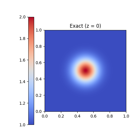
Figure 1: Reference conductivity $\gamma_{*}$ at $z=0$

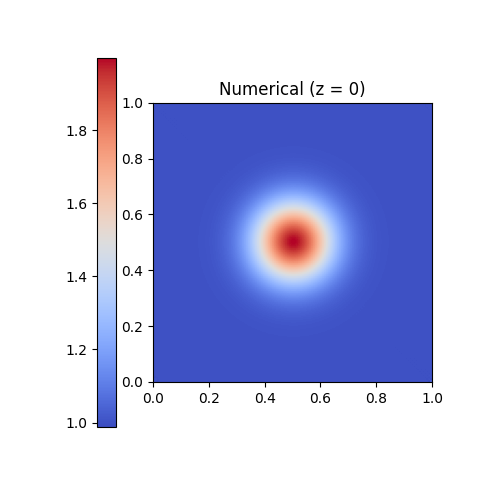
Figure 2: Reconstructed conductivity at $z=0$

Figure 3: $A$ given by (5.2). The resulting transport equation is linear. Ran for 10 iterations on a mesh of size 150 x 150 x 1.

Example 1. For our first example we choose $A$ to be

(5.2) $$A(\gamma)\ \ =\ \ \begin{bmatrix}\gamma&0&0\\ 0&\gamma&0\\ 0&0&1\end{bmatrix}$$

and reference medium $\gamma_{*}$ to be the Gaussian curve independent of $z$:

$$\gamma_{*}=\exp{\left(-\frac{(x-0.5)^{2}}{0.02}-\frac{(y-0.5)^{2}}{0.02}\right)}+1.$$

In this case the transport equation (4.6) for $\gamma_{k+1}$ becomes

$$\begin{cases}\nabla\cdot(\gamma_{k+1}(E_{k}\times B_{0}))=\nabla\cdot(\gamma_{*}(E_{*}\times B_{0})),&\text{in }\Omega\\ \gamma_{k+1}=\gamma_{*},\hfill&\text{ on }\partial\Omega^{-},\end{cases}$$

which is 2D linear isotropic, as was studied previously in [8]. To solve this linear transport equation, we use a discontinuous Galerkin (DG) method with upwinding, which we now describe briefly. Given a mesh $T_{h}$ of $\Omega$, we let $V$ be a finite dimensional space containing functions not necessarily continuous across mesh elements. We define the ‘upwinding’ term on the boundary of a triangle by

$$\bar{E}_{k}=0.5((E_{k}\times B_{0})\cdot\vec{n}+|(E_{k}\times B_{0})\cdot\vec{n}|)$$

and denote the jump of a function on an internal edge $E$ by

$$[[f]]=f^{+}-f^{-},$$

where $f^{+}$ ($f^{-}$) is its restriction to the edge from the outflow (inflow) direction, respectively. Then the variational formulation for the numerical transport problem is:

find $\gamma_{k+1}=\gamma\in V$ such that, for all $v\in V$,

$$\int_{\partial\Omega}v\gamma(E_{k}\times B_{0})\cdot\vec{n}\,ds+\sum_{E}\int_{E}[[v]][[\gamma\bar{E}_{k}]]\,dS-\int_{\Omega}\nabla v\cdot\gamma(E_{k}\times B_{0})\,dx=\int_{\Omega}F(\gamma^{*})v\,dx,$$

where $F(\gamma^{*})$ is the source data (5.1). Note that the upwinding term provides numerical stability. We refer to [14] for more details on DG methods and upwinding. Figure 3 shows the true $\gamma_{*}$, plotted alongside its numerical reconstruction using the above algorithm.

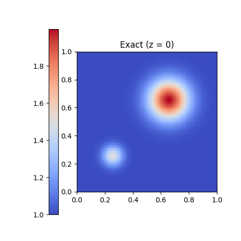
Figure 4: Reference conductivity $\gamma_{*}$ at $z=0$

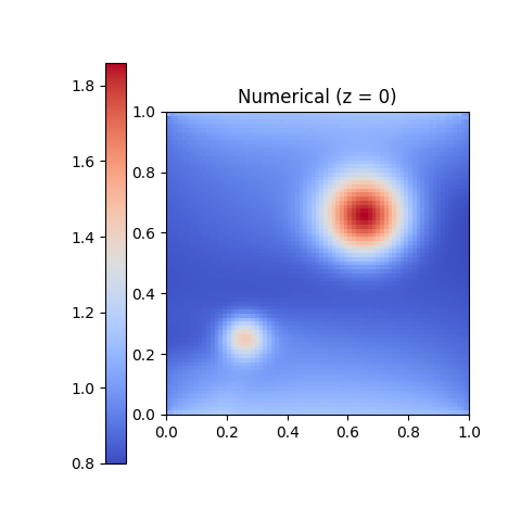
Figure 5: Reconstructed conductivity at $z=0$

Figure 6: $A$ given by (5.3), resulting in transport equation (5.4). Ran for 10 iterations on a mesh of size 75 x 75 x 10.

Example 2. In this next example we add nonlinearity in the dependence of A on $\gamma$. To solve the transport equation (4.6) in this and all of the examples that follow, instead of DG, we use the Fenics nonlinear solver with higher order Lagrange elements. We choose here

(5.3) $$A(\gamma)\ \ =\ \ \begin{bmatrix}0.4(\gamma+1)^{2}&0.01&0\\ 0.01&3\gamma&0\\ 0&0&\gamma\end{bmatrix}$$

and reference conductivity $\gamma_{*}$ to be a sum of Gaussian curves given by

$$\gamma_{*}=\exp{\left(-\frac{(x-0.65)^{2}}{0.02}-\frac{(y-0.65)^{2}}{0.02}\right)}+0.5*\exp{\left(-\frac{(x-0.25)^{2}}{0.05}-\frac{(y-0.25)^{2}}{0.05}\right)}.$$

With the definitions above, the transport problem (4.6) becomes the nonlinear equation for $\gamma=\gamma_{k+1}$:

(5.4) $$a_{1}\gamma^{2}+a_{2}\gamma+a_{3}\gamma\gamma_{x}+a_{4}\gamma_{x}-a_{5}\gamma_{y}+c=F(\gamma_{*}),\qquad\text{ in }\quad\Omega,$$

with inflow condition $\gamma=\gamma_{*}$ on $\partial\Omega^{-}$, where the spatially varying coefficients are functions of $E=[E_{1},E_{2},E_{3}]^{T}$, given by $a_{1}=0.4E_{2,x}$, $a_{2}=0.8E_{2,x}-3E_{1,y}$, $a_{3}=a_{4}=0.8E_{2}$, $a_{5}=3E_{1}$ and $c=0.4E_{2,x}$. We show the reconstruction in Figure 6.

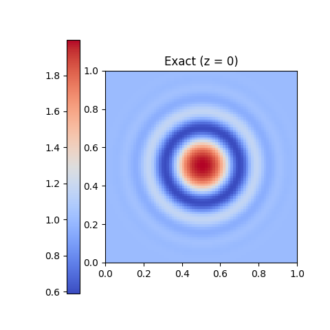
Figure 7: Reference conductivity $\gamma_{*}$ at $z=0$

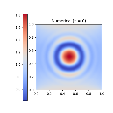
Figure 8: Reconstructed conductivity at $z=0$

Figure 9: A given by (5.5), yielding transport equation (5.6). Ran for 10 iterations on a mesh of size 75 x 75 x 10.

Example 3. In this next example we add nonlinearity on the off diagonals. Let

(5.5) $$A(\gamma)\ \ =\ \ \begin{bmatrix}0.4(\gamma+1)^{2}&0.01\gamma(1-\gamma)&0\\ 0.01\gamma(1-\gamma)&3\gamma&0\\ 0&0&\gamma\end{bmatrix}$$

and let $\gamma_{*}$ be given by

$$\gamma_{*}(x,y)=\cos{(75(x-0.5)^{2}+75(y-0.5)^{2})}\exp{\left(-\frac{(x-0.5)^{2}}{2}-\frac{(y-0.5)^{2}}{2}\right)}+1.$$

In this case the transport equation (4.6) for $\gamma_{k+1}=\gamma$ becomes:

(5.6) $$a_{1}\gamma^{2}+a_{2}\gamma\gamma_{y}+a_{3}\gamma_{y}+a_{4}\gamma+a_{5}\gamma_{x}+a_{6}\gamma\gamma_{x}+c=F(\gamma_{*}),\qquad\text{in}\quad\Omega,$$

with $\gamma=\gamma_{*}$ on $\partial\Omega^{-}$, where the coefficients are given by $a_{1}=0.4E_{2,x}+0.01E_{1,x}-0.01E_{2,y}$, $a_{2}=0.898E_{2}$, $a_{3}=0.01E_{2}-3E_{1}$, $a_{4}=0.8E_{2,x}-0.01E_{1,x}+0.01E_{2,y}-3E_{1,y}$, $a_{5}=0.8E_{2}-0.01E_{1}$, $a_{6}=0.02E_{1}$, and $c=0.4E_{2,x}$. Reconstruction results are in Figure 9.

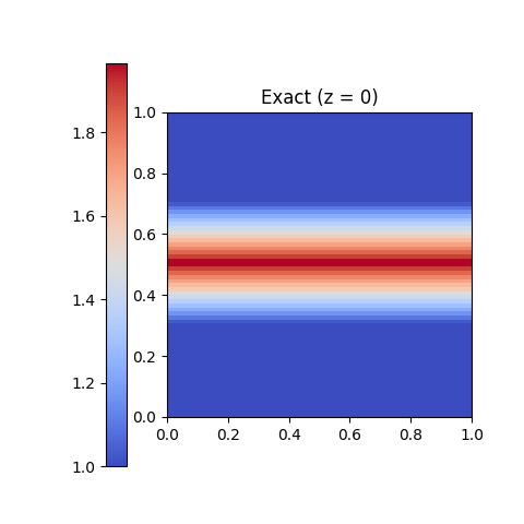
Figure 10: Reference conductivity $\gamma_{*}$ at $z=0$

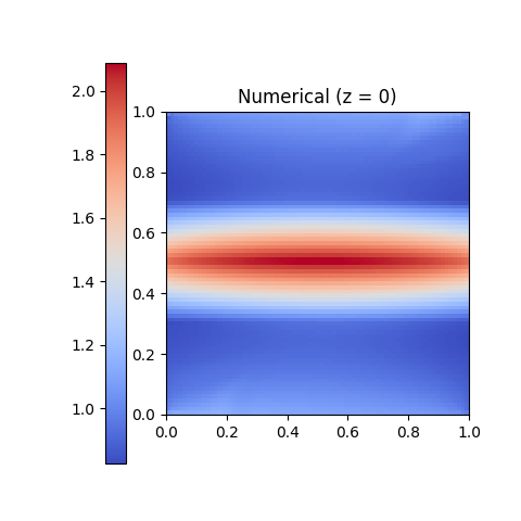
Figure 11: Reconstructed conductivity at $z=0$

Figure 12: A given by (5.7). Ran for 10 iterations on a mesh of size 75 x 75 x 10.

Example 4. Here we choose a piecewise affine $\gamma_{*}$ to test the reconstruction of non smooth conductivity. Let

(5.7) $$A(\gamma)\ \ =\ \ \begin{bmatrix}0.4(\gamma+1)^{2}&\frac{1}{\gamma+20}&0\\ \frac{1}{\gamma+20}&3\gamma&0\\ 0&0&\gamma\end{bmatrix}$$

and define $\gamma_{*}$ by

$$\gamma_{*}(x,y)=\begin{cases}1+5(x-0.3)&,\ \ \ 0.3\leq x\leq 0.5\\ 2-5(x-0.5)&,\ \ \ 0.5\leq x\leq 0.7\\ 1&,\ \ \ \text{else}\end{cases}$$

With the definitions above, the transport problem (4.6) becomes: find $\gamma=\gamma_{k+1}$ such that

(5.8) $$(E_{2,x}-E_{1,y})\gamma+(E_{2})\gamma_{x}-\left(\frac{E_{2}}{(\gamma+20)^{2}}+E_{1}\right)\gamma_{y}\\ +\left(\frac{1}{\gamma+20}\right)\left(E_{2,y}-E_{1,x}+\frac{E_{1,x}}{\gamma+20}\right)=F(\gamma^{*}),\qquad\text{in}\quad\Omega,$$

with $\gamma=\gamma_{*}$ on $\partial\Omega^{-}$. Numerical reconstructions are show in Figure 12.

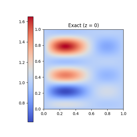
Figure 13: Reference conductivity $\gamma_{*}$ at $z=0$

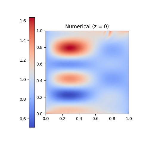
Figure 14: Reconstructed conductivity at $z=0$

Figure 15: A given by (5.9). Ran for 10 iterations on a mesh of size 100 x 100 x 10.

Example 5. Next we choose $A$ to be spatially varying as well as dependent on $\gamma$, as follows,

(5.9) $$A(\vec{x},\gamma)\ \ =\ \ \begin{bmatrix}0.4(\gamma+1)^{2}&0.25(x^{2}+y^{2})\gamma&0\\ 0.25(x^{2}+y^{2})\gamma&3\gamma&0\\ 0&0&\gamma\end{bmatrix}$$

and we let $\gamma_{*}$ be the trigonometric function

$$\gamma_{*}(x,y)=\sin(10x)\sin(5y)\sin(7(1-x))\sin(y-1)+1.$$

Numerical results are given in Figure 15.

Example 6. Finally, we present an example in which $A$ is spatially varying as well as dependent on $\gamma$ and $\gamma_{*}$ is z-dependent . We let

(5.10) $$A(\vec{x},\gamma)\ \ =\ \ \begin{bmatrix}0.4(\gamma+1)^{2}&0.25((x-0.5)^{2}+(y-0.5)^{2})\gamma&0\\ 0.25((x-0.5)^{2}+(y-0.5)^{2})\gamma&3\gamma&0\\ 0&0&\gamma\end{bmatrix}$$

and we let $\gamma_{*}$ be a piecewise constant corresponding to a spherical inclusion, that is,

$$\gamma_{*}(x,y,z)=\begin{cases}2\ ,&(x-0.5)^{2}+(y-0.5)^{2}+(z-0.5)^{2}\leq 0.4\\ 1\ ,&\text{else}\end{cases}.$$

Slices of the three dimensional reconstruction are shown in Figures 16 - 20.

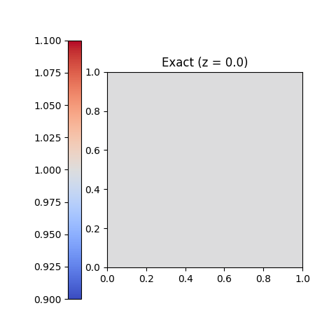
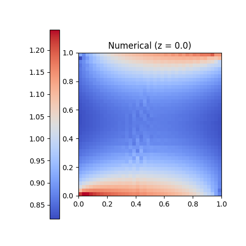
Figure 16: Reconstruction for (5.10) at $z=0$.

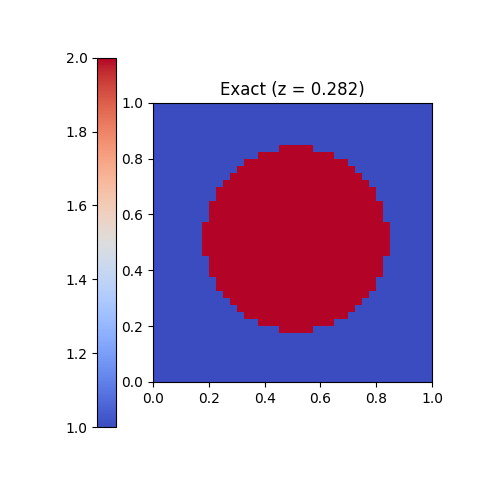
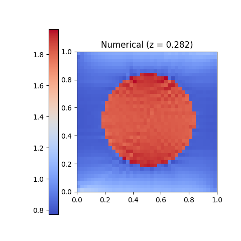
Figure 17: Reconstruction for (5.10) at $z=0.282$.

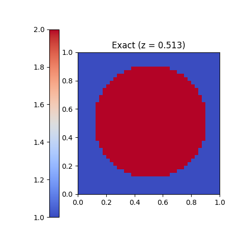
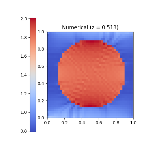
Figure 18: Reconstruction for (5.10) at $z=0.513$.

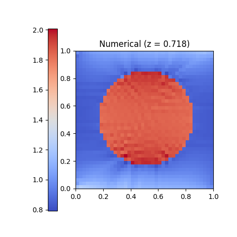
Figure 19: Reconstruction for (5.10) at $z=0.718$.

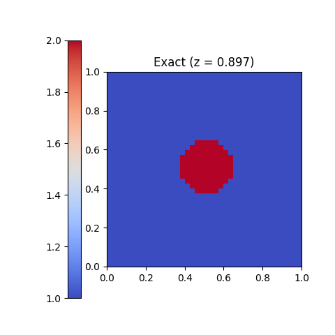
Figure 20: Reconstruction for $A$ given by the $z$-dependent (5.10) for $z=0.897$. Ran for 10 iterations on a mesh of size 40 x 40 x 40.

6 Conclusions

In this work we studied issues of stability and reconstruction of the anisotropic conductivity $\sigma$ of a biological medium $\Omega\subset\mathbb{R}^{3}$ by the hybrid inverse problem of Magneto-Acoustic Tomography with Magnetic Induction MAT-MI. More specifically, we considered a class of conductivities which correspond to a one-parameter family of symmetric and uniformly positive matrix-valued functions $t\mapsto A(x,t)$, which are a-priori known to depend nonlinearly on $t\in[\lambda^{-1},\lambda]$. This gives rise to the family of anisotropic conductivities $A(x,\gamma(x))$, $x\in\Omega$, for which the goal is to stably reconstruct the scalar function $\gamma$ in $\Omega$. We showed that if $A$ belongs to certain classes of admissible anisotropic structures, then a Lipschitz type stability estimate of the scalar function $\gamma$ from the data given by and internal functional, holds true. In particular, the argument for our theoretical framework requires that $\gamma$ and $A$ belong to $C^{1,\beta}$. Our stability estimates extend the results in [8] to the case where $\sigma$ depends nonlinearly on $\gamma$, hence allowing us to consider a more realistic type of anisotropic structures. Furthermore, we showed that the convergence of the reconstruction algorithm introduced in [8] extends to this nonlinear case, and demonstrated its effectiveness in several numerical experiments.

Several questions remain, including, as mentioned in [8], the reconstruction of full anisotropy, which we expect will require more measurements at hand. It will also be interesting to investigate more precisely to what extent the regularity assumptions considered in this paper are needed for the convergence of the reconstruction algorithm in practice; and the related question of when one needs to actually regularize the iterates by invoking the projections into the convex set $\tilde{S}$. These questions are the subject of future work.

References

- [1] G. Alessandrini, Singular solutions of elliptic equations and the determination of conductivity by boundary measurements, J. Differential Equations, 84 (2) (1990), 252-272.
- [2] G. Alessandrini and E. Cabib, Determining the anisotropic traction state in a membrane by boundary measurements, Inverse Problems and Imaging 1 (3) (2007), 437-442.
- [3] G. Alessandrini, M. De Hoop and R. Gaburro, Uniqueness for the electrostatic inverse boundary value problem with piecewise constant anisotropic conductivities, Inverse Problems 33 (2018), 125013.
- [4] G. Alessandrini, M. V. de Hoop, R. Gaburro and E. Sincich, EIT in a layered anisotropic medium, Inverse Problems and Imaging 12 (3) (2018), 667 - 676.
- [5] G. Alessandrini and R. Gaburro, Determining conductivity with special anisotropy by boundary measurements, SIAM J. Math. Anal. 33 (2001), 153-171.
- [6] G. Alessandrini and R. Gaburro, The local Calderón problem and the determination at the boundary of the conductivity, Comm. Partial Differential Equations. 34 (2009), 918-936.
- [7] H. Ammari, An introduction to mathematics of emerging biomedical imaging, Math. Appl. (Berlin) 62, Springer, Berlin, 2008.
- [8] H. Ammari, L. Qiu, F. Santosa W. Zhang, Determining anisotropic conductivity using diffusion tensor imaging data in magneto-acoustic tomography with magnetic induction, Inverse Problems,33 (12) (2017).
- [9] S. R. Arridge, Optical tomography in medical imaging, Inverse Problems 15 (2) (1999), R41.
- [10] K. Astala, M. Lassas and L. Päivärinta, Calderón inverse problem for anisotropic conductivity in the plane, Comm. Partial Differential Equations 30 (2005), 207-224.
- [11] G. Bal, Hybrid inverse problems and internal functionals, in Inverse problems and applications: inside out. II, Math. Sci. Res. Inst. Publ. 60, Cambridge University Press, Cambridge, UK (2013), 325-368.
- [12] M. I. Belishev, The Calderón problem for two-dimensional manifolds by the BC-Method, SIAM J. Math. Anal. 35 (1) (2003), 172–182.
- [13] L. Borcea, Electrical impedance tomography, Inverse Problems 18 (2002), R99-R136.
- [14] S.C. Brenner, L.R Scott, The Mathematical Theory of Finite Element Methods, Text In Applied Mathematics, Springer, (2007).
- [15] D.C. Barber, B.H. Brown, Applied potential tomography, J. Phys. E. Sci. Instrum. 17 (1984) 723–733.
- [16] A. P. Calderón, On an inverse boundary value problem, Seminar on Numerical Analysis and its Applications to Continuum Physics (Rio de Janeiro, 1980), 65–73, Soc. Brasil. Mat., Rio de Janeiro, 1980. Reprinted in: Comput. Appl. Math. 25 (2-3) (2006), 133–138.
- [17] W. Craggs, Applied Mathematical Sciences, The Mathematical Gazette,57 (399) (1973).
- [18] S. Foschiatti, R. Gaburro and E. Sincich, Stability for the Calderon’on’s problem for a class of anisotropic conductivities via an ad hoc misfit functional, Inverse Problems 37 (2021), 125007.
- [19] R. Gaburro and W. R. B. Lionheart, Recovering Riemannian metrics in monotone families from boundary data, Inverse Problems 25 (4) (2009).
- [20] R. Gaburro and E. Sincich, Lipschitz stability for the inverse conductivity problem for a conformal class of anisotropic conductivities, Inverse Problems 31 015008 (2015).
- [21] A. Greenleaf, M. Lassas, and G. Uhlmann, Anisotropic conductivities that cannot be detected by EIT, Physiological measurement 24 (2) (2003), 413.
- [22] D. Gilbarg, N. Trudinger, Elliptic Partial Differential Equations of Second Order, The Mathematical Gazette, Springer, (1998).
- [23] D. Holder, Electrical Impedance Tomography, Bristol: Institute of Physics Publishing, (2005)
- [24] D. Isaacson, J. C. Newell,J .C. Goble, M. Cheney, Thoracic impedance images during ventilation, Annu. Conf. IEEE Eng. Med. Biol. Soc. 12, (1990) 106–107.
- [25] D. Isaacson, J. Mueller, S. Siltanen, Biomedical applications of electrical impedance tomography, Physiol. Meas. 24, (2003), 391–638.
- [26] J. Jossinet, The impedivity of freshly excised human breast tissue, Physiol.Meas. 19, (1998), 61–75.
- [27] R. Kohn and M. Vogelius, Identification of an unknown conductivity by means of measurements at the boundary, SIAM-AMS Proc. 14 (1984), 113-123.
- [28] P. Kuchment, Mathematics of hybrid imaging: a brief review, in The Mathematical Legacy of Leon Ehrenpreis, Springer Proc. Math. 16, Springer, Milan, 2012, 183-208.
- [29] L. Mariappan, G. Hu, B. He, Magnetoacoustic tomography with magnetic induction for high-resolution bioimepedance imaging through vector source reconstruction under the static field of MRI magnet, Medical Physics,41 (2) (2014).
- [30] O. G. Martinsen et al, Interface phenomena and dielectric properties of biological tissue, Encyclopedia of surface and Colloid Science, (7) (2002).
- [31] R. Langer, An inverse problem in differential equations, Bull. Amer. Math. Soc. 39 (1933) 814–820.
- [32] M. Lassas and G. Uhlmann, On determining a Riemannian manifold from the Dirichlet-to-Neumann map, Ann. Sci. École Norm. Sup. 34 (2001), 771-787.
- [33] M. Lassas, G. Uhlmann and M. Taylor, The Dirichlet-to-Neumann map for complete Riemannian manifolds with boundary, Comm. Anal. Geom. 11 (2) (2003), 207-221.
- [34] J. M. Lee and G. Uhlmann, Determining anisotropic real-analytic conductivities by boundary measurements, Comm. Pure Appl. Math. 42 (1989), 1097-1112.
- [35] W. R. B. Lionheart, Conformal uniqueness results in anisotropic electrical impedance imaging, Inverse Problems 13 (1997), 125-134.
- [36] L. Qiu, F. Santosa, Analysis of the magnetoacoustic tomography with magnetic induction, SIAM Journal on Imaging Sciences,8 (3) (2015).
- [37] L. Slitchter, An inverse boundary value problem in electrodynamics, Phys. 4 (1933) 411–418.
- [38] S. Stefanesco, C. Schlumberger, M. Schlumberger, Sur la distribution électrique autour d’une prise de terre ponctuelle dans un terrain a couchés horizontales, homogènes et isotropes, J. Phys. Radium Ser. 7 (1930), 132–140.
- [39] J. Sylvester, An anisotropic inverse boundary value problem, Comm. Pure. Appl. Math. 43 (1990), 201-232.
- [40] A.N. Tikhonov, Uniqueness of the solution for the problem of electrical prospecting, Dokl. Akad. Nauk SSSR 69 (1949) 780–797.
- [41] G. Uhlmann, Electrical impedance tomography and Calderón’s problem (topical review), Inverse Problems 25 (12) (2009), 123011 doi:10.1088/0266-5611/25/12/123011.
- [42] T. Widlak and O. Scherzer, Hybrid tomography for conductivity imaging, Inverse Problems 28 (2012), 084008.
- [43] Y. Xu, B. He, Magnetoacoustic tomography with magnetic induction (MAT-MI), Physics in Medicine and Biology,50 (21) (2005).
- [44] Y. Zou, Z. Guo, A review of electrical impedance techniques for breast cancer detection, Med. Eng. Phys. 25, (2003), 79–90.