Understanding star formation in molecular clouds

Probability distribution functions of the total hydrogen column density (N-PDFs) are a valuable tool for distinguishing between the various processes (turbulence, gravity, radiative feedback, magnetic fields) governing the morphological and dynamical structure of the interstellar medium. We present N-PDFs of 29 Galactic regions obtained from Herschel imaging at high angular resolution (18^′′), covering diffuse and quiescent clouds, and those showing low-, intermediate-, and high-mass star formation (SF), and characterize the cloud structure using the $\Delta$-variance tool. The N-PDFs show a large variety of morphologies. They are all double-log-normal at low column densities, and display one or two power law tails (PLTs) at higher column densities. For diffuse, quiescent, and low-mass SF clouds, we propose that the two log-normals arise from the atomic and molecular phase, respectively. For massive clouds, we suggest that the first log-normal is built up by turbulently mixed H₂ and the second one by compressed (via stellar feedback) molecular gas. Nearly all clouds have two PLTs with slopes consistent with self-gravity, where the second one can be flatter or steeper than the first one. A flatter PLT could be caused by stellar feedback or other physical processes that slow down collapse and reduce the flow of mass toward higher densities. The steeper slope could arise if the magnetic field is oriented perpendicular to the LOS column density distribution. The first deviation point (DP), where the N-PDF turns from log-normal into a PLT, shows a clustering around values of a visual extinction of A_V (DP1)$\sim$2-5. The second DP, which defines the break between the two PLTs, varies strongly. In contrast, the width of the N-PDFs is the most stable parameter, with values of $\sigma$ between $\sim$0.5 and 0.6. Using the $\Delta$-variance tool, we observe that the A_V value, where the slope changes between the first and second PLT, increases with the characteristic size scale in the $\Delta$-variance spectrum. We conclude that at low column densities, atomic and molecular gas is turbulently mixed, while at high column densities, the gas is fully molecular and dominated by self-gravity. The best fitting model N-PDFs of molecular clouds is thus one with log-normal low column density distributions, followed by one or two PLTs.

1 Introduction

Important tools for characterizing molecular clouds are probability distribution functions of density ($\rho$-PDF) and column density (N-PDF) because they can be directly linked to theories of the star formation process (e.g., Padoan et al., 1997, 2002; Vázquez-Semadeni & Garcia, 2001; Hennebelle & Chabrier, 2008, 2009; Federrath & Klessen, 2012; Burkhart, 2018). Numerical simulations that include or exclude particular physical processes (such as solenoidally or compressively driven turbulence, radiative feedback, gravity, and magnetic fields) show that the shape of the N-PDF strongly depends on the dominant process and the evolutionary state of the cloud. For example, the N-PDF is purely log-normal if the cloud structure is governed only by isothermal supersonic turbulence and develops a power law tail (PLT) under self-gravity (e.g., Klessen, 2000; Vázquez-Semadeni & Garcia, 2001; Dib & Burkert, 2005; Kritsuk et al., 2011; Collins et al., 2012; Girichidis et al., 2014; Ward et al., 2014; Burkhart et al., 2015a; Veltchev et al., 2016; Mocz et al., 2017; Auddy et al., 2018; Veltchev et al., 2019; Körtgen et al., 2019; Krumholz & McKee, 2020; Jaupart & Chabrier, 2020; Donkov et al., 2021). The slope of the PLT changes during the evolution of the cloud and can depend on the 2D projection (Ballesteros-Paredes et al., 2011; Cho et al., 2011; Federrath & Klessen, 2013; Burkhart, 2018). In addition, Schneider et al. (2015c) report the detection of two PLTs in massive star-forming regions where the second PLT in the high-column-density regime, characterizing small spatial scales (sub-parsec to a few parsec), is flatter than the first one. They argue that this is caused by a physical process that slows down collapse and reduces the flow of mass toward higher densities. Possible processes are rotation of collapsing cores, which introduces an angular momentum barrier (Khullar et al., 2021), increasing optical depth and weaker cooling, magnetic fields, geometrical effects, and protostellar feedback. Though such a flatter PLT was first found in a simulation presented by Kritsuk et al. (2011), it is only recently that there are theoretical explanations for this phenomenon (Jaupart & Chabrier, 2020; Donkov et al., 2021). Jaupart & Chabrier (2020) develop an analytical theory of the density PDF and attribute the second PLT to free-fall collapse of a dense region in a cloud. Donkov et al. (2021) propose that the thermodynamic state of the gas changes from isothermal on large scales to polytropic with an exponent larger than 1 on the sub-parsec proto-stellar core scale. In the hydrodynamics models of Khullar et al. (2021), the second PLT appears only at much higher densities and small (sub-parsec) scales, and corresponds to rotationally supported material, for example a disc.

Numerical simulations of supersonic, isothermal turbulence have demonstrated that the variance of logarithmic density fluctuations, expressed by the width of the density PDF, $\sigma_{\rho}$, in a compressible, turbulent medium correlates with the RMS sonic Mach number, $\mathcal{M}$, and the type of forcing of the turbulence. The forcing can be parameterized by the so-called forcing parameter $b$, which encodes the relative amount of stirring versus compression in the turbulence, with $\sigma_{\rho}^{2}$=$\ln$(1 + $b^{2}\mathcal{M}^{2}$) (Federrath et al., 2008). This variance - Mach relation also holds for column densities seen in isothermal simulations (Burkhart et al., 2012) and hydrodynamic models without self-gravity (Beattie et al., 2019). Molina et al. (2012) extended this expression by including the ratio between thermal and magnetic energies, expressed as $\beta_{mag}$, and obtained $\sigma_{\rho}^{2}$=$\ln$(1 + ($b^{2}\mathcal{M}^{2}\,\beta_{mag}/(1+\beta_{mag})))$.

In recent years, observations using extinction maps (e.g., Lombardi et al., 2008; Kainulainen et al., 2009; Froebrich et al., 2010; Spilker et al., 2021) or Herschel column density maps (e.g., Schneider et al., 2012, 2013, 2015a; Russeil et al., 2013; Alves de Oliveira et al., 2014; Tremblin et al., 2014; Stutz & Kainulainen, 2015; Benedettini et al., 2015) started to test the theoretical predictions. The interpretation of the observed N-PDF shapes, however, varies strongly. For example, while Butler et al. (2014) propose that N-PDFs of extinction maps of infrared dark clouds (IRDCs) are best fitted by log-normal distributions, Schneider et al. (2015b) find a pure power law distribution for the same clouds. Moreover, Brunt (2015), studying low-mass clouds, advocate that the PLT is a part of a log-normal N-PDF arising from the cold, molecular part of the cloud. Gravity as the dominant process behind forming PLTs in star-forming regions is suggested by the observational studies of Froebrich et al. (2010) and Schneider et al. (2013, 2015a). In contrast, Kainulainen et al. (2011) propose that pressure due to different phases in the interstellar medium gives rise to the PLT. Tremblin et al. (2014), on the other hand, argue that the N-PDF of clouds closely associated with H II regions can show a more complex shape with several bumps and PLTs due to radiative feedback effects that cause compression of local gas into shells and pillars. More recently, Planck polarization observations at 353 GHz have been used to identify that the relative orientations between the column density structure and the magnetic field orientation are also related to the PLTs (Soler, 2019).

It is not only the nature of the high column density part of the N-PDF that is strongly debated, but also that of the low column density range. While the observational studies mentioned above mostly find a log-normal distribution for star-forming and non-star-forming clouds for low column densities, Alves et al. (2017) claim that there is no observational evidence for log-normal N-PDFs of molecular clouds but that they are well described by power laws. Various authors (Schneider et al., 2015a; Ossenkopf et al., 2016; Chen et al., 2018; Körtgen et al., 2019), however, discuss the impact of observational limitations such as noise, line-of-sight (LOS) effects, and incompleteness on the N-PDF but show that there are efficient methods to correct for noise and contamination. They conclude that a log-normal and PLT part of the N-PDF is the best-fitting model for star-forming clouds.

These rather different views raise the need for a statistical approach to understand N-PDFs, covering diffuse and quiescent regions to high-mass regions. We thus started a series of papers, of which the first one (Paper I, Schneider, Ossenkopf, Csengeri et al. 2015a) investigates how line-of-sight contamination affects N-PDFs. The second one (Paper II, Schneider, Klessen, Csengeri et al. 2015b) studies N-PDFs of massive IRDCs and shows by using complementary molecular line data that the power law distribution of the N-PDF can be explained by local and global infall of gas. And finally, the third study, Paper III (Schneider, Bontemps, Motte et al. 2016), discusses the problems of N-PDFs constructed from molecular line observations.

The objective of this paper is to present N-PDFs for a significant number of molecular clouds with varying SF activity, using dust column density maps derived from Herschel imaging only. Though there are methods that combine data from Herschel, extinction maps and Planck data (e.g., Lombardi et al., 2014; Butler et al., 2014; Zari et al., 2016; Abreu-Vicente et al., 2017; Pokhrel et al., 2020), we prefer to employ only Herschel maps at 18^′′ angular resolution, in particular because we do not study the extended cloud environment. Such analyses would involve Planck and extinction maps, and we do not want to introduce systematic effects by using several data sets that require a cross-calibration and could introduce a bias. The high angular resolution of our maps enables us to better resolve the high column density part of the N-PDF that is constituted by molecular clumps and cores on a parsec and sub-parsec scale. We study the variation of the N-PDF shapes for diffuse, quiescent, low-, intermediate-, and high-mass SF regions. We also establish a well-defined data set of molecular cloud parameters that can be used for further studies such as linking the density structure with the dynamics of the gas, the SF rate and efficiency, the magnetic field and the core mass function. Our main goals are:
Quantifying the average column density, total mass, and LOS confusion for Galactic molecular clouds;
Providing the characteristics of the N-PDF such as PLT slope(s), widths of the log-normal part(s), the first deviation point (DP1) from the log-normal to PLT distribution and the second deviation point (DP2) from the first PLT to the second for this set of molecular clouds;
Investigating how cloud morphology (for instance filamentary vs. spherical) and stellar feedback (such as expanding H II region bubbles) influences the N-PDF shape;
Calculating the $\Delta$-variance spectrum (Ossenkopf et al., 2008a) to characterize the structural variation in the column density map;
Assessing if there are (column) density thresholds that signify a change in the dominant physical process or chemistry, such as the transition from turbulence to gravity or the transition from atomic to molecular hydrogen.

The current paper is organized the following way: Section 2 briefly describes how we derived the Herschel column density maps (Sect. 2.1), chose the sample of molecular clouds (Sect. 2.2), estimated LOS confusion (Sect. 2.3), and determined the N-PDFs and the $\Delta$-variance (Sect. 2.4). Section 3 presents the column density maps and the resulting cloud parameters (density, mass, etc.), the N-PDFs, and the $\Delta$-variance of the observed clouds. Section 4 assesses the value of N-PDFs as an analysis tool and describes what they tell us about the column density structure of molecular clouds. Section 5 summarizes the main findings of this paper.

2 Observations and data analysis

Table 1: Overview of the molecular cloud sample, ordered by cloud type and name.

Cloud	$\alpha_{J2000}$	$\delta_{J2000}$	Distance	Geometry	References
	[h:m:s]	[∘:′:′′]	[kpc]
High-mass SF regions
Cygnus North	20:37:54	41:44:57	1.40	ridge+filaments	Hennemann et al. (2012); Schneider et al. (2016)
Cygnus South	20:35:08	39:41:50	1.40	filaments+pillars	Schneider et al. (2016)
M16	18:19:40	-13:47:34	2.00	filaments+pillars	Hill et al. (2012); Tremblin et al. (2013, 2014)
M17	18:18:36	-16:34:39	2.20	clumps	this paper
NGC 6334	17:20:58	-35:51:45	1.35	massive ridge	Russeil et al. (2013); Tiegé et al. (2017)
NGC 6357	17:25:06	-34:25:57	1.75	dispersed clumps	Russeil et al. (2019)
NGC 7538	23:14:02	61:26:48	2.80	evolved bubble	Fallscheer et al. (2013)
Rosette	06:33:32	04:15:23	1.46a	H II bubble/	Motte et al. (2010); Hennemann et al. (2010)
				ridge	Schneider et al. (2010); DiFrancesco et al. (2010)
					Schneider et al. (2012); Cambrésy et al. (2013)
					Tremblin et al. (2013, 2014)
Vela C	09:00:37	-43:56:50	0.70	ridge	Hill et al. (2011); Giannini et al. (2012)
					Minier et al. (2013); Tremblin et al. (2014)
Intermediate-mass SF regions
Aquila	18:29:43	-02:46:49	0.436b	bipolar filament	Könyves et al. (2010, 2015); André et al. (2010)
					Bontemps et al. (2010a, b); Schneider et al. (2013)
Mon R2	06:06:45	-06:17:01	0.862	hub-filament	Didelon et al. (2015); Pokhrel et al. (2016)
					Rayner et al. (2017)
Mon OB1	06:32:00	10:30:00	0.80	massive clump	this paper
NGC 2264	06:40:24	09:25:52	0.719c	ridge+filaments	Nony et al. (2021)
Orion B	05:48:54	00:48:08	0.40	filaments	Schneider et al. (2013); Könyves et al. (2020)
Serpens	18:34:59	00:00:00	0.436b	filaments+clumps	Roccatagliata et al. (2015); Fiorellino et al. (2021)
Low-mass SF regions
Cham I	10:55:42	-77:07:31	0.192d	ridge	Alves de Oliveira et al. (2014)
Cham II	12:38:45	-78:29:35	0.198d	clumps	Alves de Oliveira et al. (2014)
IC5146	21:48:48	47:29:16	0.813b	filament	Arzoumanian et al. (2011); Roy et al. (2015)
Lupus I	15:41:03	-34:05:34	0.182	filaments+clumps	Rygl et al. (2013); Benedettini et al. (2015, 2018)
Lupus III	16:10:03	-39:04:40	0.162c	filaments+clumps	Rygl et al. (2013); Benedettini et al. (2015, 2018)
Lupus VI	16:04:36	-42:04:24	0.204	filament+clumps	Rygl et al. (2013); Benedettini et al. (2015, 2018)
Perseus	03:35:41	31:31:56	0.235b	filament+clumps	Sadavoy et al. (2012, 2014)
					Pezzuto et al. (2012, 2021)
Pipe	17:23:08	-26:24:07	0.145	filament+clumps	Peretto et al. (2012); Roy et al. (2014, 2015)
$\rho$Oph	16:27:31	-24:12:40	0.140b	clumps	Roy et al. (2014); Ladjelate et al. (2020)
Taurus	04:21:00	27:46:45	0.14	filaments	Kirk et al. (2013); Marsh et al. (2014, 2016a)
					Palmeirim et al. (2013)
Quiescent regions
Cham III	12:38:45	-78:29:35	0.16	clumps	Alves de Oliveira et al. (2014)
Musca	12:27:36	-71:38:53	0.15	filament	Cox et al. (2016); Bonne et al. (2020)
Polaris	01:50:35	88:21:10	0.489a	network filaments	Menshchikov et al. (2010); Schneider et al. (2013)
					Miville-Deschenes et al. (2010)
					Ward-Thompson et al. (2010); André et al. (2010)
Diffuse/atomic regions
Draco	16:47:57	61:45:16	0.60	clumps	Miville-Deschenes et al. (2017), this paper

Table 2: Global molecular cloud parameters from Herschel column density and temperature maps, ordered by cloud type and name.

Cloud	LOS	$\langle N({\rm H_{2}})\rangle$	A1	$R$	$\langle n\rangle$	$M_{1}$
	dust		AV$>$1		AV$>$1	AV$>$1
	[mag]	[1021cm${}^{-2}]$	[pc2]	[pc]	[cm-3]	[103 M⊙]
	(1)	(2)	(3)	(4)	(5)	(6)
High-mass SF regions
Cygnus North	5.0	5.06	3417	33.0	24.9	324.46
Cygnus South	5.0	5.47	3731	34.5	25.7	383.45
M16	7.8	4.18	1057	18.3	36.9	87.12
M17	6.6	9.99	2478	28.1	57.7	483.76
NGC 6334	8.7	13.98	882	16.8	135.1	238.60
NGC 6357	4.2	7.22	1004	17.9	65.4	145.14
NGC 7538	3.3	4.22	1524	22.0	31.0	130.39
Rosette	1.1	4.10	881	16.8	39.7	70.64
Vela C	2.0	6.85	450	12.0	92.7	58.00
Intermediate-mass SF regions
Aquila	2.5	2.74	445	11.9	37.3	25.94
Mon R2	1.6	2.00	82	5.1	63.3	4.60
Mon OB1	2.2	2.31	59	4.4	86.1	4.87
NGC 2264	1.6	2.60	169	7.3	57.5	11.12
Orion B	0.9	2.06	683	14.8	22.7	29.69
Serpens	1.6	1.46	266	10.8	21.9	14.15
Low-mass SF regions
Cham I	0.25	1.07	18	2.4	72.5	0.767
Cham II	0.23	1.00	12	2.0	82.2	0.507
IC5146	0.37	1.07	121	6.2	28.0	5.03
Lupus I	0.17	0.82	6.6	1.4	91.7	0.364
Lupus III	0.44	1.16	5.0	1.3	148.9	0.180
Lupus VI	0.46	1.00	7.3	1.5	106.0	0.398
Perseus	0.66	1.62	174	7.4	35.3	4.350
Pipe	0.59	1.72	40	3.6	77.8	1.452
$\rho$Oph	1.25	1.57	26	2.9	89.0	1.244
Taurus	0.4	1.73	97	5.5	50.7	4.03
Quiescent regions
Cham III	0.16	0.81	9.4	1.7	75.4	0.317
Musca	0.37	0.75	3.2	1.0	121.2	0.110
Polaris	0.31	1.73	11.3	1.9	31.9	1.208
Diffuse/atomic regions
Dracoa		0.60	1500	21.9	4.4	8.04

2.1 Column density maps from Herschel

For this study, we use the cloud sample from Herschel key programs, the Herschel Gould Belt survey (HGBS, André et al. (2010)) and the Herschel imaging survey of OB Young Stellar objects (HOBYS, Motte et al. (2010)), as well as data from open time programs such as the Herschel Infrared GALactic plane survey (Hi-GAL, Molinari et al. (2010)) and individual PI programs. Most of the column density maps used in this paper were already published (see references in Table 1 for Herschel imaging observations for each region), either at an angular resolution of 18^′′ or 36^′′.

All column density maps were determined from a pixel-to-pixel graybody fit to the red wavelength of PACS (Poglitsch et al., 2010) at 160 $\mu$m (13.5^′′ angular resolution) and all SPIRE (Griffin et al., 2010) wavelengths (250 $\mu$m, 350 $\mu$m, 500 $\mu$m at 18.2^′′, 24.9^′′, and 36.3^′′ resolution, respectively). For the SPIRE data reduction, we used the HIPE pipeline (versions 10 to 13), including the destriper task for SPIRE, and HIPE and scanamorphos (Roussel, 2013) for PACS. The SPIRE maps were calibrated for extended emission. All maps have an absolute flux calibration, either by using offset values determined as described in Bernard et al. (2010) for the sources of the Gould Belt and HOBYS program, or using the zeroPointCorrection task in HIPE for SPIRE and IRAS maps for PACS for the remaining clouds. For the SED fit, we fixed the specific dust opacity per unit mass (dust+gas) approximated by the power law $\kappa_{\nu}$=0.1$\,(\nu/1000{\rm GHz})^{\beta_{d}}$ cm²/g with $\beta_{d}$=2, and left the dust temperature and column density as free parameters (see Hill et al., 2011; Russeil et al., 2013; Roy et al., 2013, for details). The procedure underpinning how high angular resolution maps were obtained is described in detail in Appendix A of Palmeirim et al. (2013). The concept is to employ a multiscale decomposition of the flux maps and assume a constant LOS temperature. The final map at 18^′′ resolution is constructed from the difference maps of the convolved SPIRE maps (at 500 $\mu$m, 350 $\mu$m, and 250 $\mu$m) and the temperature information from the color temperature derived from the 160 $\mu$m to 250 $\mu$m ratio.

The Draco region has very weak emission so that we used the classical fitting technique (SED fit to 160 $\mu$m to 500 $\mu$m) to determine column density maps at 36^′′ resolution to obtain the best signal-to-noise ratios. In addition, data points at each wavelength were weighted with a calibration uncertainty of 10% and 20% for SPIRE and PACS, respectively. For the star-forming and quiescent molecular clouds, we used a value of 3.4$\times$10^-25 cm^-2/H for the coefficent $\kappa_{\nu}$, which is in the range of typical values (Ossenkopf & Henning, 1994) from 1.75$\times$10^-25 cm^-2/H for compact grains in diffuse interstellar clouds to 5.0$\times$10^-25 cm^-2/H for fluffy grains with ice mantles in dense molecular cores. For Draco, we expect rather diffuse cloud conditions without much ice accretion or dust coagulation. Based on Planck observations, Juvela et al. (2015) derived $\kappa_{\nu}$=2.16$\times$10^-25 cm^-2/H for such regions, following the standard interstellar reddening behavior, so we use this value for Draco. For the diffuse cloud Draco, which is mostly atomic, we calculated the total hydrogen column density using $N$=A_V$\times$1.87$\times$10²¹ cm^-2 mag^-1 (Bohlin et al., 1978). For all other clouds, which are mostly molecular, we transformed H₂ column density into visual extinction, using the conversion formula $N({\rm H_{2}})$=A_V$\times$0.94$\times$10²¹ cm^-2 mag^-1.

The uncertainty in the Herschel column density maps arise from the uncertainty in the assumed form of the opacity law, including variations of dust content and dust properties across the clouds and possible temperature gradients along the LOS. The total uncertainty is estimated to be around $\sim$30–50% (see above and, e.g., Russeil et al., 2013, for a discussion). By comparing an extinction map and the Herschel column density map of Rosette, Cambrésy et al. (2013) argued that the optical depth from dust emission close to heating sources like massive clusters might be overestimated. Their extinction map, however, suffers from saturation at values above A_V$\sim$20 (only 2MASS) and $\sim$35 (2MASS combined with other near-IR or mid-IR data), respectively. This limitation makes the study of very dense regions such as the centers of high-mass SF clouds impossible using extinction maps. The multi-temperature column density mapping procedure PPMAP (Marsh et al., 2016b) produces differential column density maps, using Herschel flux maps, in a number of temperature intervals. The PPMAP method, however, includes the 70 $\mu$m data in the SED fit in addition to the 160-500 $\mu$m wavelength data, but the 70 $\mu$m is mostly tracing hot dust from cloud surfaces and not the cool bulk of the atomic and molecular gas in which we are interested.

Apart from the overall uncertainty of the column density maps, there is observational noise in the maps, arising from the SPIRE and PACS instrumental noise. We estimate the noise level in the final column density maps, using the full N-PDF for regions that are hardly affected by LOS-contamination and that are sufficiently extended. As was shown in Ossenkopf et al. (2016), noise produces excess in the low column density part of the N-PDF and increases the width of the log-normal part. When the noise amplitude is less than 40% of the peak column density, the excess in the N-PDF at low column densities is linear. As we see later (Sec. 3.2), the N-PDFs with the highest dynamical range at low column densities indeed show this linear tail. These N-PDFs go down to values below an A_V of 0.1 (e.g., Chamaeleon I-III, Lupus I, Musca, Polaris, Draco). We perform a fit including an error tail, a log-normal part, and possbile PLTs, following Ossenkopf et al. (2016) and described in the next section, and derive as extreme values an error level of A_V of $\sim$0.02 for Draco and $\sim$0.1 for Polaris. Because all sources were observed in the same way (scanning speed, instrumental setup, etc.), we assume to first order that all maps, including those of the star-forming clouds, have a similar low noise level.
If there is too much LOS-confusion or the maps are not extended enough to cover areas without cloud emission, the noise cannot be estimated this way. We thus take the maximum noise level for Polaris (A_V=0.1) as a standard value for all maps of star-forming clouds and conclude that the observational noise is low enough to resolve a major fraction of the low column density part with A_V$<$1 of the N-PDF, at least for the low-mass and quiescent clouds. It should be noted that noise also shifts the peak of the N-PDF toward higher column densities (Ossenkopf et al., 2016).

2.2 The molecular cloud sample

A total of 29 cloud complexes were selected for our study, and their coordinates and distances are listed in Table 1, together with references for Herschel publications. For the distances, we use values from the literature and update with recent results from GAIA. A large overview on distance estimates based on a combination of stellar photometric data with GaiaDR2 parallax measurement is given in Zucker et al. (2020). However, they give multiple distance estimates across a single cloud with sometimes large differences, so that we prefer to keep the typical values from the literature. For the N-PDFs shape, the accurate distances are not relevant, they only play a role in the mass determination. Complementary to other N-PDF studies (Kainulainen et al., 2009; Froebrich et al., 2010; Lombardi et al., 2008; Alves et al., 2017), we include more distant and massive clouds that form intermediate- to high-mass stars, and quiescent clouds with apparently no SF, and employ only Herschel data.

Generally, throughout the paper, we use the following nomenclature (Bergin & Tafalla, 2007, e.g.): Low-mass regions are molecular clouds with a mass of 10³–10⁴ M_⊙, and a size of up to a few tens of parsecs that typically form stars of low mass (examples are Taurus or Perseus). High-mass regions are giant molecular clouds (GMCs) with a mass of 10⁵–10⁶ M_⊙, a size of up to a $\sim$100 pc, and observational signatures of high-mass SF and cluster formation (such as Cygnus). GMCs in addition sometimes contain regions defined as ridges (Schneider et al., 2010; Hennemann et al., 2012; Nguyen-Luong et al., 2011, 2013; Didelon et al., 2015; Motte et al., 2018) that are massive, gravitationally unstable filamentary structures of high column density (typically N${}_{\rm H_{2}}>$10²³ cm^-2) with high-mass SF. Some clouds fall in between these categories as they have masses in the range of 10⁴–10⁵ M_⊙ and form mainly low- and intermediate-mass stars but also some high-mass stars (such as Orion B). For simplicity, we classify these as intermediate-mass regions. Quiescent clouds are those that show very little SF activity (no or only very few protostars or prestellar cores. Finally, diffuse clouds are mostly atomic.

2.3 Line-of-sight contamination

Column density maps from Herschel can be affected by LOS confusion, in particular in the Galactic plane and along spiral arms. Unrelated dust emission from LOS clouds can add to the observed flux in the different wavelength ranges and thus the column density determined from Herschel can be overestimated. In Paper I, we studied in detail the influence of such confusion on the maps and the N-PDFs and introduced a simple correction method to determine the typical background and foreground contribution from the maps in regions outside the bulk emission of the target. This approach was then further investigated and justified in Ossenkopf et al. (2016). Summarizing, it was shown that contamination by foreground and background emission can be safely removed as a constant screen if the contaminating N-PDF is log-normal (see Sec. 2.4.1 for the nomenclature), and its width $\sigma_{\eta,cloud}$ is narrow, typically $<$0.5$\,\sigma_{\eta,cloud}$, or the column density of the contaminant is sufficiently small. We thus applied the same method as in Paper I and measured the contamination from a rectangular polygon placed out of the molecular cloud close to the map borders. We used the procedure developed in Ossenkopf et al. (2016) to obtain a separate N-PDF from these pixels within the polygon and derived the peak value and width of the contaminating N-PDF. Appendix A (Figs. A.1. and A.2) shows an example of this method applied to the Aquila cloud. For all maps used here, the peak of this N-PDF corresponds within 10% to the values obtained from averaging the pixels in the rectangular regions. The widths of the contaminating N-PDFs $\sigma_{\eta,cont}$ are small and vary between $\sigma_{\eta,cont}$=0.05 and $\sigma_{\eta,cont}$=0.19 so that the ratio $\sigma_{\eta,cont}$/$\sigma_{\eta,cloud}$ varies between 0.09 and 0.42. The ratio between the contamination column density and cloud peak column density $N_{cont}$/$N_{peak}$ is mostly below 1, the smallest value is 0.41, only three maps have a value of around 3. From Figs. 5 and 6 in Appendix A, we see that even if the column density ratio $N_{cont}$/$N_{peak}$ is high, the ratio of the contaminating and cloud N-PDF widths $\sigma_{\eta,cont}$/$\sigma_{\eta,cloud}$ is always so small that we can conclude that the LOS correction by removing a constant screen is indeed a valid method for our clouds. The values determined in this way are listed in Table 2. It is important to note that LOS contamination of several log-normal N-PDFs does not create multiple peaks but instead broadens and shifts the column density distribution.

Massive clouds that are not too distant and more isolated, such as Rosette, have a low contamination level (A_V$\sim$4) while other GMCs such as M16 have a high level of A_V$\sim$8. Extreme cases are IRDCs that are far away (typically more than several kpc) because the IRDC is an intrinsic part of the larger-scale molecular cloud. NGC6334 is problematic because there is no consistent concensus on the amount of contamination as discussed in Russeil et al. (2013). From molecular line data and the Herschel image, we derive a value of around A_V=6, while Froebrich et al. (2010) deduce a higher extinction (between A_V=7 and 14). The reason for this discrepancy is probably a strong spatial variation of the contamination due to several clouds along the LOS. Therefore, the derived parameters for mass and the N-PDF for NGC6334 should be treated with care. For the Cygnus X North and South regions, we independently determined the average extinction of the ”Cygnus Rift”, a feature lying in front of Cygnus at distances $\ll$1 kpc, to be A_V$\sim$5 (Schneider et al., 2007). We thus use this value as an approximation for the contamination.

”Over-correction” of LOS-contamination can also lead to unrealistic features in the N-PDF for high-mass SF clouds but still provides more reliable estimates for average column densities and masses and the slope of the PLT than using values without any correction. Intermediate-mass clouds such as Aquila, Vela, and MonOB1 are also affected by LOS-contamination. The absolute values of the contamination are low, typically around an A_V of 2, and the width of the contaminating N-PDF is small. Low-mass regions show not much LOS confusion with values of A_V$<$2.

All LOS-values derived from the dust maps are upper limits because the Herschel maps are not always extended enough so that the cloud borders (if something like a ”border” exists) are sufficiently covered. Accordingly, the polygons may still be placed in areas of extended cloud emission. On the other hand, one must stay close to the cloud area because a more remote polygon would not trace the same LOS, thereby risking to calibrate our correction methods on contaminants that do not affect our column density maps.

2.4 Statistical analysis tools

2.4.1 Probability distribution functions of column density (N-PDFs)

Probability distribution functions (PDFs) form the basis for modern theories of SF (Dib et al., 2007; Hennebelle & Chabrier, 2008, 2009; Federrath & Klessen, 2012; Padoan et al., 2014; Burkhart, 2018; Burkhart & Mocz, 2019), and are frequently used as an analysis tool for simulations and observations. We determine the PDFs expressed in column density $N$ or visual extinction A_V  (we note that $N\propto{\rm A}_{\rm v}$) and call it N-PDF, following Myers (2015). The probability of finding gas within a range [A_V, A_V+dA_V] is given by the surface-weighted N-PDF of the extinction with $\int_{{\rm A}_{\rm v}}^{{\rm A}_{\rm v}+d{\rm A}_{\rm v}}$ $p_{{\rm A}_{\rm v}}({\rm A}^{\prime}_{\rm v})\,d{\rm A}^{\prime}_{\rm v}$, where $p_{{\rm A}_{\rm v}}({\rm A}_{\rm v})$ corresponds to the PDF of the extinction. We define

$$\eta\equiv\rm ln\frac{A_{\rm v}}{\langle A_{\rm v}\rangle},$$ (1)

as the natural logarithm of the visual extinction A_V  divided by the mean extinction $\langle{\rm A}_{\rm v}\rangle$. The quantity $p_{\eta}(\eta)$ then corresponds to the probability distribution function of $\eta$, and by definition

$$\int_{-\infty}^{+\infty}p_{\eta}{\rm d\eta}=\int_{0}^{+\infty}p_{A_{\rm v}}\rm dA_{\rm v}=1.$$ (2)

In Paper I, we showed that a binsize of 0.1 in $\eta$ provides the best compromize between resolving small features in the N-PDF and avoiding low-number pixel statistics. We tested four methods to characterize the N-PDF and derive its characteristic properties. In the following, we briefly summarize the methods, but we only use the values derived with method 4 for the paper.

All methods except method 3 fit a log-normal function at the low column density range with

$$p_{\eta}\,{\rm d}\eta=\frac{1}{\sqrt{2\pi\sigma_{\eta}^{2}}}{\rm exp}\Big{[}-\frac{(\eta-\mu)^{2}}{2\sigma_{\eta}^{2}}\Big{]}{\rm d}\eta,$$ (3)

where $\sigma_{\eta}$ is the dispersion and $\mu$ is the mean logarithmic column density. For the high column density range, a single or several PLTs are fitted. There are, however, subtle differences in these methods:

Method 1 used in Paper I performs several fits on a grid of parameters for $\eta$ and $\mu$ and then calculates the positive and negative residuals. Then, the range of log-normality is determined under the premise that the difference between the model and $p_{\eta}$ is less than three times the statistical noise in $p_{\eta}$ and we derive the width and peak of the log-normal part of the N-PDF. We then perform a linear regression fit to determine the slope(s) $s$ of the PLT(s). The slope values that are fitted start at the deviation point (DP) where the log-normal N-PDF turns into one or two power law distribution(s) and stop where the power law is no longer well defined (at high column densities) due to a low-number pixel statistics caused by resolution effects.

Method 2 follows Ossenkopf et al. (2016) and fits an error slope at very low column densities, followed by a log-normal distribution and a single PLT at high column densities. This method includes numerical error weighting and map size errors. We tested a large parameter space and obtained the most reliable results for a 10% map size error.

Table 3: Parameters from the N-PDFs study from Herschel column density maps, ordered by cloud type and name.

Cloud	Model	AV,pk1	AV,pk2	$\sigma_{\rm\eta 1}$	$\sigma_{\rm\eta 2}$	DP1	DP2	$s_{1}$	$s_{2}$
		[mag]	[mag]			[mag]	[mag]
	(1)	(2)	(3)	(4)	(5)	(6)	(7)	(8)	(9)
High-mass SF regions
Cygnus N	ELL2P	2.63	2.76	0.52	1.04	18.5	79.7	-1.83	-1.40
Cygnus S	ELL2P	1.39	3.46	0.29	0.52	15.2	37.5	-2.37	-2.66
M16	ELLP	3.17	3.55	0.33	0.79	8.1	-	-2.47	-
M17	ELL2P	4.63	12.85	0.79	0.47	37.2	87.5	-2.67	-1.70
NGC 6334	ELL2P	4.90	14.95	0.81	0.37	28.1	68.3	-2.18	-1.55
NGC 6357	ELL2P	2.77	9.88	0.74	0.45	26.4	45.5	-2.57	-3.11
NGC 7538	ELL2P	1.75	3.13	0.33	0.74	9.0	18.5	-1.44	-2.00
Rosette	ELL2P	3.03	9.09	0.63	0.49	17.3	35.9	-1.95	-3.82
Vela C	ELL2P	4.64	3.80	0.25	1.13	33.8	65.5	-3.68	-4.59
mean		3.2$\pm$1.2	7.1$\pm$4.4	0.52$\pm$0.21	0.67$\pm$0.26	21.5$\pm$9.8	54.8$\pm$22.5	-2.35$\pm$0.60	-2.60$\pm$1.08
median		3.0	3.8	0.52	0.52	18.5	55.5	-2.37	-2.33
Intermediate-mass SF regions
Aquila	ELL2P	1.42	2.77	0.57	0.35	4.6	19.1	-2.10	-2.38
Mon R2	ELL2P	0.84	1.71	0.36	0.52	3.1	14.6	-1.79	-1.15
Mon OB1	ELL2P	0.21	1.75	0.49	0.90	4.8	10.9	-1.03	-3.48
NGC 2264	ELL2P	1.64	1.62	0.47	1.07	6.2	16.2	-2.00	-1.27
Orion B	ELL2P	1.53	1.66	0.10	0.46	3.6	43.3	-1.99	-3.64
Serpens	ELL2P	0.66	1.43	0.67	0.53	5.1	30.1	-1.76	-2.00
mean		1.1$\pm$0.5	1.8$\pm$0.4	0.44$\pm$0.18	0.64$\pm$0.26	4.6$\pm$1.0	22.4$\pm$11.1	-1.77$\pm$0.35	-2.32$\pm$0.97
median		1.1	1.68	0.47	0.52	4.7	17.7	-1.88	-2.19
Low-mass SF regions
Cham I	EL2P	0.47	-	0.85	-	2.35	6.0	-0.90	-3.57
Cham II	ELL2P	0.54	0.72	0.43	1.06	2.7	26.9	-2.36	-4.27
IC5146	ELL2P	0.71	0.82	0.37	0.79	3.4	9.6	-1.47	-2.76
Lupus I	ELL2P	0.44	0.63	0.29	0.76	1.6	4.4	-1.39	-2.77
Lupus III	ELL2P	0.91	0.93	0.36	0.84	4.8	5.9	-3.49	-2.41
Lupus IV	ELL2P	0.72	1.12	0.24	0.40	2.1	9.5	-2.14	-2.88
Perseus	L2P	1.04	-	0.35	-	1.4	3.9	-1.55	-2.03
Pipe	ELL2P	0.99	1.92	0.29	0.34	5.2	13.4	-2.91	-1.72
$\rho$Oph	LL2P	0.32	1.04	0.26	0.48	2.3	16.2	-1.27	-2.37
Taurus	LL2P	0.64	1.51	0.28	0.51	2.7	18.8	-2.27	-4.40
mean		0.7$\pm$0.2	1.1$\pm$0.4	0.37$\pm$0.17	0.65$\pm$0.24	2.9$\pm$1.2	11.5$\pm$7.0	-2.00$\pm$0.77	-2.92$\pm$0.85
median		0.7	0.99	0.32	0.64	2.5	9.5	-1.85	-2.76
Quiescent regions
Cham III	ELL2P	0.53	0.64	0.43	0.80	3.5	12.1	-3.83	-2.02
Musca	LL2P	0.45	0.70	0.23	0.20	0.9	4.1	-1.73	-5.05
Polaris	ELL2P	0.45	0.62	0.38	0.61	2.35	3.4	-4.08	-2.34
mean		0.48$\pm$0.04	0.65$\pm$0.03	0.35$\pm$0.08	0.54$\pm$0.25	2.3$\pm$1.1	6.6$\pm$4.0	-3.21$\pm$1.05	-3.14$\pm$1.36
median		0.45	0.64	0.38	0.61	2.35	4.1	-3.83	-2.34
Diffuse/atomic regions
Draco	LL	0.13	0.40	0.32	0.34	-	-	-	-

Table 4: Parameters from the $\Delta$-variance study from Herschel column density maps, ordered by cloud type and name.

Cloud	$\beta_{1}$	P1	$\beta_{2}$	P2
		[pc]		[pc]
	(1)	(2)	(3)	(4)
High-mass SF regions
Cygnus N	2.51	0.59	-	-
Cygnus S	2.17	1.42	-	-
M16	2.17	2.62	-	-
M17	2.22	2.57	-	-
NGC 6334	2.41	1.10	-	-
NGC 6357	2.02	2.53	-	-
NGC 7538	2.93	2.10	-	-
Rosette	2.42	4.76	-	-
Vela C	2.30	1.83	-	-
mean	2.35$\pm$0.25	2.17$\pm$1.13	-
median	2.30	2.10	-	-
Intermediate-mass SF regions
Aquila	2.28	0.32	2.62	3.90
Mon R2	2.20	0.37	3.04	1.37
Mon OB1	3.38	0.76	2.50	4.36
NGC 2264	2.80	0.98	-	-
Orion B	2.18	1.39	2.36	4.90
Serpens	2.36	0.79	-	-
mean	2.53$\pm$0.43	0.92$\pm$0.50	2.63$\pm$0.25	3.63$\pm$2.35
median	2.32	0.79	2.56	4.13
Low-mass SF regions
Cham I	2.95	0.21	2.78	2.61
Cham II	2.64	0.61	2.90	2.56
IC5146	2.50	0.68	-	-
Lupus I	2.77	0.11	2.45	0.82
Lupus III	3.10	0.08	2.66	1.18
Lupus VI	2.99	0.79	2.63	6.53
Perseus	2.13	2.45	-	-
Pipe	3.04	0.25	-	-
$\rho$Oph	2.17	0.17	2.62	1.39
Taurus	3.30	0.30	-	-
mean	2.76$\pm$0.37	0.55$\pm$0.67	2.67$\pm$0.14	2.51$\pm$1.91
median	2.86	0.28	2.64	1.96
Quiescent regions
Cham III	2.73	0.45	-	-
Musca	3.42	0.11	2.55	0.89
Polaris	2.40	0.15	-	-
mean	2.85$\pm$0.42	0.24$\pm$0.15	2.55	0.89
median	2.73	0.15	2.55	0.89
Diffuse/atomic regions
Draco	2.27	5.95	-	-

Method 3, the adapted BPlfit (Veltchev et al., 2019), calculates the slope of a power law part of an arbitrary distribution, without any assumption about the functional form of other parts of this distribution and constant binning. The slope and the DP are then derived simultaneously as averaged values as the number of bins is varied. The method was elaborated further for detection of a second PLT (Marinkova et al., 2021) - this technique was also used to get the results in this paper.

Method 4 fits models that are a combination of: error slopes at low column densities (E), log-normals (L), pairs of log-normals (LL), power laws (P) and double power laws (PP). In total 8 models are considered: ELP, ELLP, EL2P, ELL2P, LP, LLP, L2P, LL2P. The number of parameters for each model ranges from 4 to 11. Error slopes contribute 2 parameters: the $\eta$ below which the error slope is fit, and the error slope itself. The log-normal contributes 2 parameters: the log-normal mean value and its width. Pairs of log-normals contribute 5 parameters: a mean and width for each log-normal and the ratio of amplitudes of the two log-normals. Each power law contributes 2 parameters: the $\eta$ value above which the power law is fit, and the power law slope. The fitting of each model is done using a Monte-Carlo Markov Chain (MCMC) to determine the maximum likelihood parameters of each model. The MCMC is performed using 500 walkers, each with 100,000 steps. Visual inspection of the walker’s paths reveal that this is sufficient to sample to likelihood distribution and find the maximum.

To determine the best fitting model out of the 8 models considered, we use the Bayesian Information Criterion (BIC):

$$\mathrm{BIC}(k) =k\ln(n)-2\ln(\mathcal{L})$$ (4)

where $n$ is the number of data points in the N-PDF, $k$ is number of model parameters, and $\mathcal{L}$ is the maximum likelihood found via the MCMC. The model with the minimum BIC is considered the best fitting model. Further, we use the BIC-weights to illustrate the evidence of one model over another. If the best-fitting model’s BIC-weight is greater than 10 times the weight of the next most likely model (an evidence ratio of greater than 10), we consider it to firmly be the best model; otherwise, we cannot exclude the second best-fitting model entirely. The BIC and BIC-weights of each model for each cloud considered can be found in Appendix B.

2.4.2 $\Delta$-variance

The $\Delta$-variance (Stutzki et al., 1998; Ossenkopf et al., 2008a, b) is a method to quantify the relative amount of structural variation in a 2D map as a function of the size scale. It measures the amount of structure on a given scale $L$ in a map $S$, which is a 2D scalar function for our column density maps, by filtering the map with a spherically symmetric wavelet $\bigcirc_{L}$:

$$\sigma^{2}_{\Delta}(L)=\langle\left(S\otimes\bigcirc_{L}\right)^{2}\rangle_{x,y},$$

where $\left\langle\ldots\right\rangle_{x,y}$ is the ensemble average over coordinates $x$ and $y$ in the column density map, and $\otimes$ is the convolution operator. The $\Delta$-variance probes the variation of the intensity $S$ over a length $L$ (called ”lag”) and thus measures the amount of structural variation on that scale. We use as a filter function the ”Mexican hat filter” with an annulus-to-core-diameter ratio of about 1.5 since it provides the best results for a clear detection of pronounced scales (Ossenkopf et al., 2008a, b). Weighting the image with the inverse noise function (1/$\sigma_{rms}$) allows us to distinguish variable noise from real small-scale structure (Bensch et al., 2001). Our Herschel column density maps, however, have such a high dynamic range and very low noise level that there is no need to include a noise map.

The $\Delta$-variance and power spectra are closely linked. For any 2D image with a power spectrum $P(k)\propto|k|^{-\beta}$, in which $k$ is the spatial frequency, the 2D $\Delta$-variance is related to the lag by a power law with $\sigma^{2}_{\Delta}\propto L^{\beta-2}$ for 0 $<\beta<$ 6. Practically, we determine the slope $\alpha$ of the $\Delta$-variance (see below) and derive thus $\beta$=$\alpha$+2. $\beta$-values range typically between 2 and 3 where numbers at the lower end indicate more structure on smaller scales and accordingly, high values imply more structure on large scales. For many regions, the $\Delta$-variance spectrum does not follow a single power law distribution but shows typically two peaks. We thus always start our fit at the resolution limit, defined by the beam size of 18^′′, until the first peak or turnover point in the spectrum to obtain a slope value for this first part and thus $\beta_{1}$. We perform a second fit, deriving $\beta_{2}$, only in cases where there is a another visible power law behavior in the $\Delta$-variance spectrum with another peak and turnover point. For the column density maps discussed here, the values of $\beta_{1}$ and $\beta_{2}$, as well as the peak and turnover point in parsec, are given in Table 3.

On the smallest scales, the $\Delta$-variance spectrum is limited by the beam size and radiometric noise and on the largest scales, it can be limited by the map size. The error bars shown in the lower right panels in Appendix C are from the Poisson statistics of each bin. The $\Delta$-variance performs much faster on rectangular maps without empty regions. Therefore, we rotated the maps, which were observed in the coordinate system of right ascension and declination (J2000), and slightly cut the edges to obtain clean borders. Due to these rotations, we display the column density maps only using offsets from the central position (Table 1) in arcmin. The calculation of the $\Delta$-variance spectrum and the fit are performed in IDL, using widget-based routines introduced in Ossenkopf et al. (2008a).

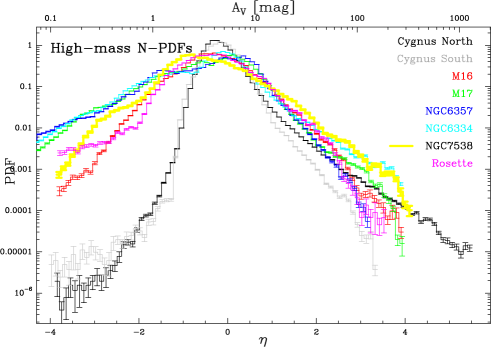
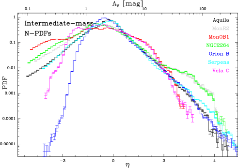
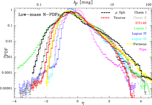
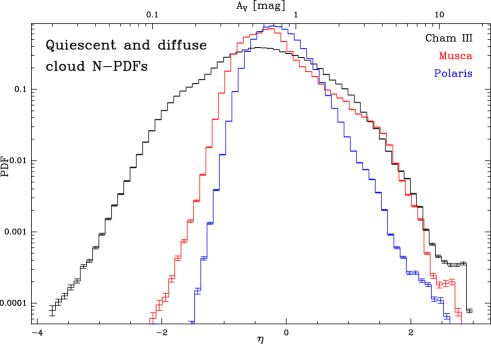
Figure 1: N-PDFs of all clouds ordered by cloud type, from high-mass and intermediate mass SF regions (top panels) to low-mass and quiescent regions (bottom panels). Each panel shows the N-PDFs for clouds in different colors. The column density is expressed in visual extinction (upper x-axis) and in $\eta$ (lower x-axis). Error bars are calculated using Poisson statistics. For better visibility, we reduced the error bars by a factor of 2 (see Figs. in Appendix C for plots with the full error bars). We note that recently, a more sophisticated method was proposed by Jaupart & Chabrier (2022) to derive the statistical error bars of PDFs employing the autocovariance function.

3 Results and Analysis

3.1 Molecular cloud parameters

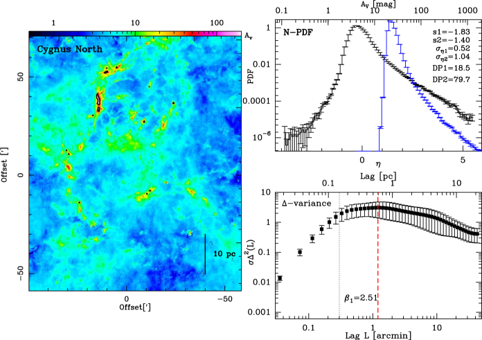
Figure 8: CYGNUS X NORTH (DR21): Left: LOS corrected column density map in visual extinction. The image is rotated and a length scale is given in the panel. For the cloud N-PDFs with two PLTs, the contour of the second DP is plotted in black. Right (lower panel): $\Delta$-variance spectrum. X-axis units are arcmin (bottom) and parsec (top). The black dashed line indicates the angular resolution (18^′′), the first red dashed line indicates the upper limit for the fit of $\beta_{1}$ (the lower limit is the resolution limit) and in case there are two fitting intervalls, two other red dashed lines indicate the fit range for $\beta_{2}$. The values of $\beta_{1}$ and $\beta_{2}$ are given in the panel. The errors are omitted for better visibility, they are always on the order of 0.01 to 0.03. Right (top panel): N-PDF of LOS corrected column density in black, expressed in visual extinction (upper x-axis) and in $\eta$ (lower x-axis). For comparison, the N-PDF of the uncorrected map is displayed in blue. The slope s of the PLT, the width $\sigma$ (expressed in $\eta$) of the log-normal part of the (corrected) N-PDF, and the deviation point DP (expressed in A_V) are given in the panel.

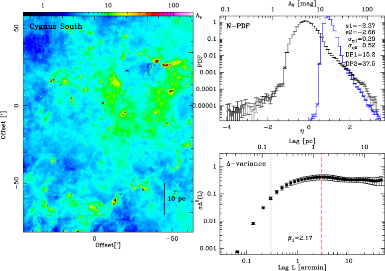
Figure 9: CYGNUS X SOUTH (DR15): Fig. caption see Fig. C.1.

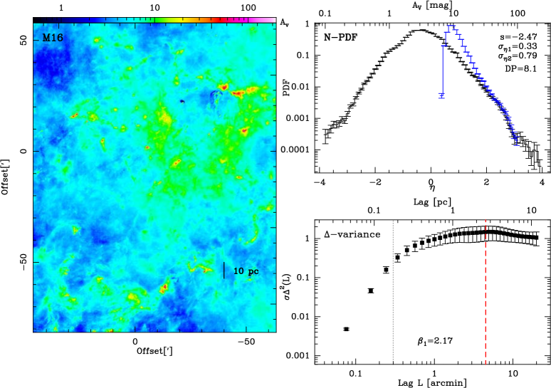
Figure 10: M16: Fig. caption see Fig. C.1.

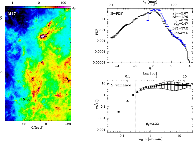
Figure 11: M17: Fig. caption see Fig. C.1.

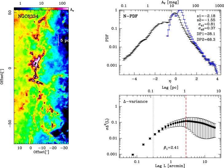
Figure 12: NGC6334: Fig. caption see Fig. C.1.

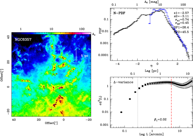
Figure 13: NGC6357: Fig. caption see Fig. C.1.

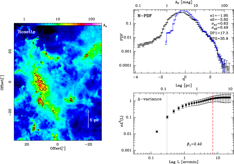
Figure 15: ROSETTE: Fig. caption see Fig. C.1.

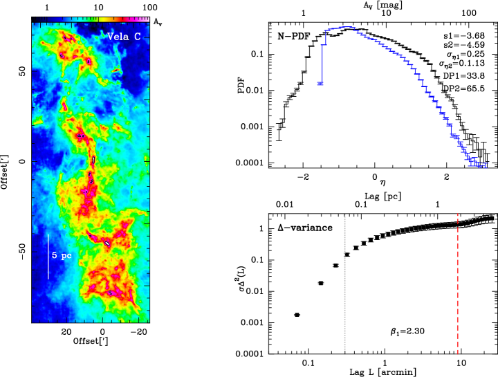
Figure 16: VELA C: Fig. caption see Fig. C.1.

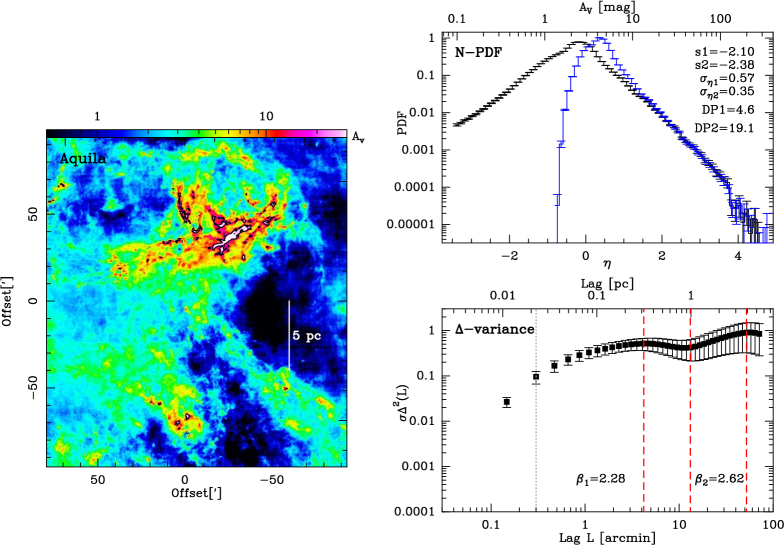
Figure 17: AQUILA: Fig. caption see Fig. C.1.

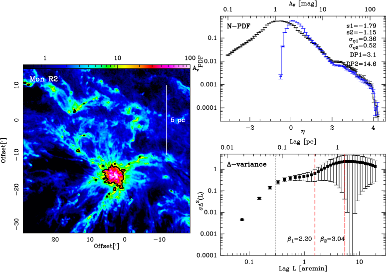
Figure 18: MONR2: Fig. caption see Fig. C.1.

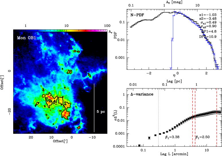
Figure 19: MONOB1: Fig. caption see Fig. C.1.

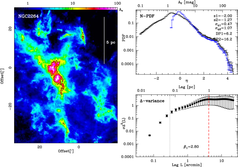
Figure 20: NGC2264: Fig. caption see Fig. C.1.

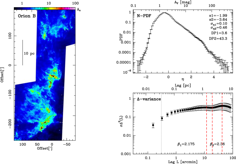
Figure 21: ORION-B: Fig. caption see Fig. C.1.

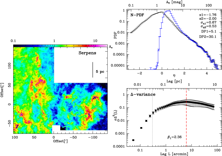
Figure 22: SERPENS: Fig. caption see Fig. C.1. For comparison, the N-PDF of the uncorrected map is displayed in grey.

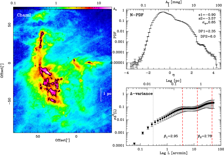
Figure 23: Chamaeleon I: Fig. caption see Fig. C.1.

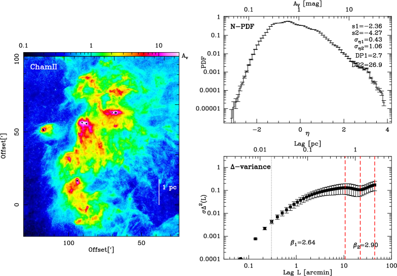
Figure 24: Chamaeleon II: Fig. caption see Fig. C.1.

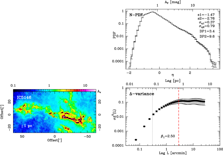
Figure 25: IC5146: Fig. caption see Fig. C.1.

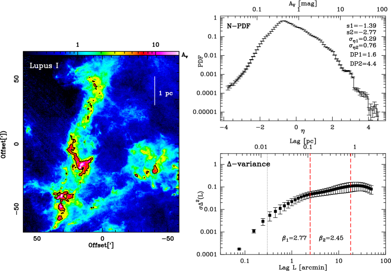
Figure 26: LUPUS I: Fig. caption see Fig. C.1.

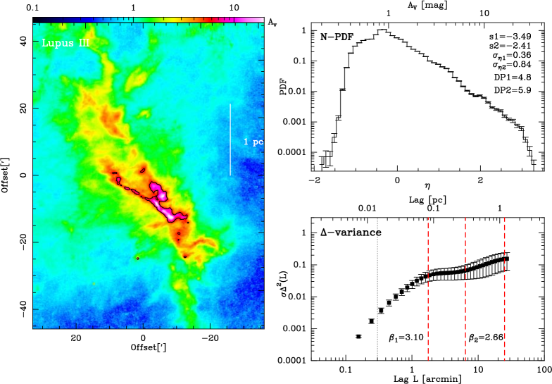
Figure 27: LUPUS III: Fig. caption see Fig. C.1.

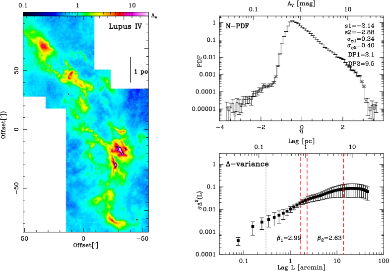
Figure 28: LUPUS IV: Fig. caption see Fig. C.1.

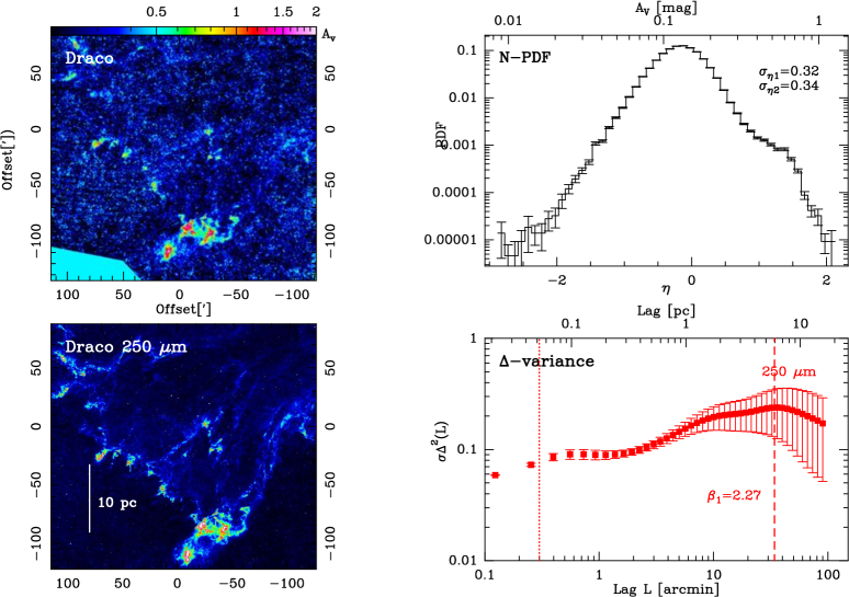
Figure 36: DRACO: Fig. caption see Fig. C.1.

In Figs. 8-36 in Appendix C, we show the column density maps of each cloud – expressed in visual extinction – together with its respective N-PDF and $\Delta$-variance spectrum. Table 2 gives cloud parameters such as average column density $\langle N({\rm H_{2}})\rangle$, as well as mass ($M$) above A_V=1 and mean density $n$. Table 3 displays the properties of the N-PDF (peak, width, DPs from log-normal to PLT and PLT to PLT, and the slopes of the PLTs) and the $\beta$-values of the $\Delta$-variance. For a better comparison to other studies (Lada et al., 2010), we use the common threshold of A_V =1 for the mass determination for all clouds except Draco, which is a diffuse region with a very low overall column density and we do not apply any threshold.

The masses given in Table 2 justify the classification of the clouds into the categories of high-, intermediate-, and low-mass. The high-mass clouds cover a range between $\sim$7$\times$10⁴ M_⊙ (Rosette) up to $\sim$5$\times$10⁵ M_⊙ (M17) and the intermediate-mass ones cover a range between $\sim$5$\times$10³ M_⊙ (MonR2, MonOB1) and $\sim$6$\times$10⁴ M_⊙ (Vela C), respectively. The low-mass clouds comprise rather different types of cloud. For example, the small Lupus regions have only a few hundred M_⊙ and show little SF activity while Taurus and Perseus are extended (more than 100 pc²) and more massive ($\sim$5$\times$10³ M_⊙). Because only low-mass stars are forming in the latter clouds, we classify them in the low-mass cloud category. The diffuse and quiescent clouds have low masses, except for Draco, which is a very extended region (around 1500 pc²). We do not compare our values of molecular cloud parameters to the ones published elsewhere (see Table 1) because we applied a LOS-correction and thus derive possibly lower values for certain clouds, and we determine the cloud parameters above A_V=1.

3.2 N-PDFs of molecular clouds

3.2.1 Shapes of the N-PDFs

Though N-PDFs from Herschel studies have been already presented in various previous publications, we show all N-PDFs from the cloud sample in this paper to present a homogeneous data set. We exclude all bins with low probability ($\sim$10^-4-10^-5) at the high column density range for fitting because otherwise, the fit would suffer from low pixel number statistics. We note that the maps are sampled on a finer grid (typically 4^′′) while the angular resolution is 18^′′ (36^′′ for Draco). The gridding, however, has no significant influence on the N-PDF, as was shown in Appendix A in Paper I, but it can lead to some bumps in the N-PDF at high column densities. Some N-PDFs exhibit a sharp drop at the very last high column density bins, which is a resolution effect. For the regions where we correct for LOS contamination, we show in Appendix C the original N-PDF (in blue) and the corrected N-PDF (in black), of which the latter is used for determination of the N-PDF parameters. In Appendix D, we display the N-PDF with the best fitting model and the residuals. The LOS-correction leads to a pronounced tail in the low-column density range (Schneider et al., 2015a; Ossenkopf et al., 2016). For clarity of display, we cut all other N-PDFs at the A_V =0.1 level, which we consider to be approximately the noise level (see Sec. 2.1).

For a first overview, Fig.1 shows all N-PDFs for each cloud type in one figure. The shapes of the N-PDFs are very complex and do not reflect the perfect examples of N-PDFs often found from simulations, typically a simple log-normal part and a PLT. Moreover, we note that the classification in log-normal parts and PLTs is only a simple analytic expression which tries to approximate the N-PDF shape. In reality, N-PDFs are probably many overlapping log-normals and PLTs, describing different areas and physical processes with deviations from log-normal due to intermittency in the turbulent fields (Federrath et al., 2010). The maps are so large with sufficient resolution that the underlying complexity is evident in the plots and the errors so small that it is clear that the models are only approximate. Nevertheless, we will try to limit the possible models and give explanations for the shapes that are physically motivated. We first order the N-PDF shapes by increasing complexity: Single/double log-normal: the diffuse region Draco; Single log-normal and double PLT with error slope: Cham I; Double log-normal and double PLT without error slope: Musca, Pipe, $\rho$Oph, Taurus; Double log-normal and double PLT with error slope and $|s_{1}|>|s_{2}|$: Cygnus North, M17, Mon R2, NGC 2264, NGC 6334, Cham III, Lupus III, Polaris, Pipe; Double log-normal and double PLT with error slope and $|s_{1}|<|s_{2}|$: Aquila, Cygnus South, Mon OB1, NGC 6357, NGC 7538, Vela C, Cham II, IC5146, Lupus I, Lupus IV, Orion B, $\rho$Oph, Serpens, Taurus

The combination of two log-normal and two PLTs is the most frequent one. We confirm the detection of a flatter second PLT than the first one ($|s_{1}|>|s_{2}|$) for Mon R2 and NGC 6334 (Schneider et al., 2015c), and find more examples (see above), for all cloud types. Furthermore, a new class of N-PDFs was detected where the second PLT is steeper than the first one ($|s_{1}|<|s_{2}|$), and this category contains clouds with low-, intermediate-, and high mass. There is thus no striking correlation between cloud type and slope(s) of the PLTs. In particular the second, flatter PLTS is not limited to massive clouds but also occurs in low-mass and quiescent clouds.

For all N-PDFs, the best fitting model is the one that contains two log-normal distributions for the lower column density range. We propose two possible explanations, depending on cloud type: in quiescent clouds and regions of low-mass SF, the two log-normal parts may represent the N-PDFs of atomic hydrogen (lowest column density range) and molecular hydrogen. For massive and intermediate mass clouds, we suggest that both peaks arise from the fully molecular gas and that the peak or bump at higher column densities is caused by stellar feedback when gas is compressed by expanding H II-region or stellar wind. We come back to this point in the next section.

3.2.2 N-PDFs of high-mass star forming clouds

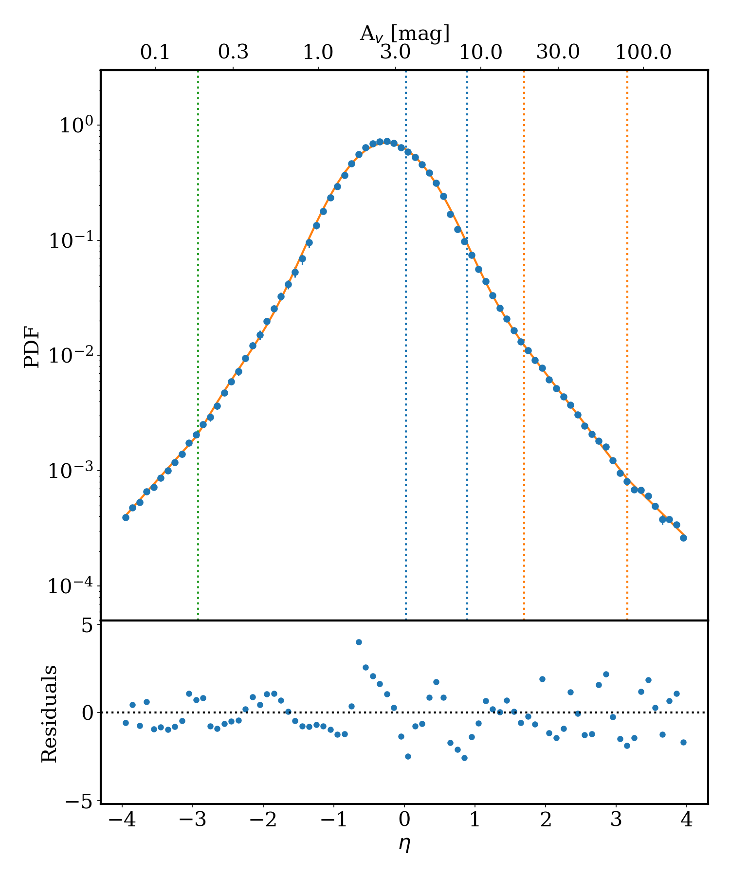
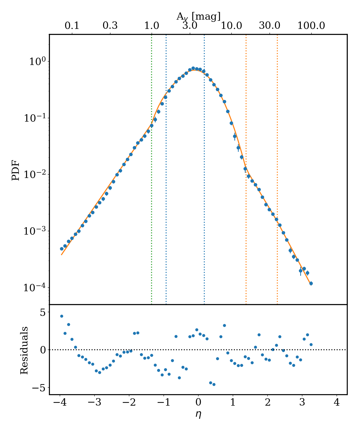
Figure 37: N-PDFs of LOS corrected column density (blue points), expressed in visual extinction (upper x-axis) and in $\eta$ (lower x-axis) of DR21 (left) and DR15 (right). The left y-axis gives the PDF (there can be small differences compared to the plots in Appendix C because for the model fit, we excluded the extreme low- and high density ranges, which leads to a slightly different normalization). The orange curve indicates the best fitting model for the N-PDF (see Table 5 and 6). The vertical lines show the peak values of the log-normal(s) in blue, the break points for the power laws in orange and the error power law break point in green. Underneath is the standardized residuals, a perfect model would give numbers with mean of 0 and a variance of 1.

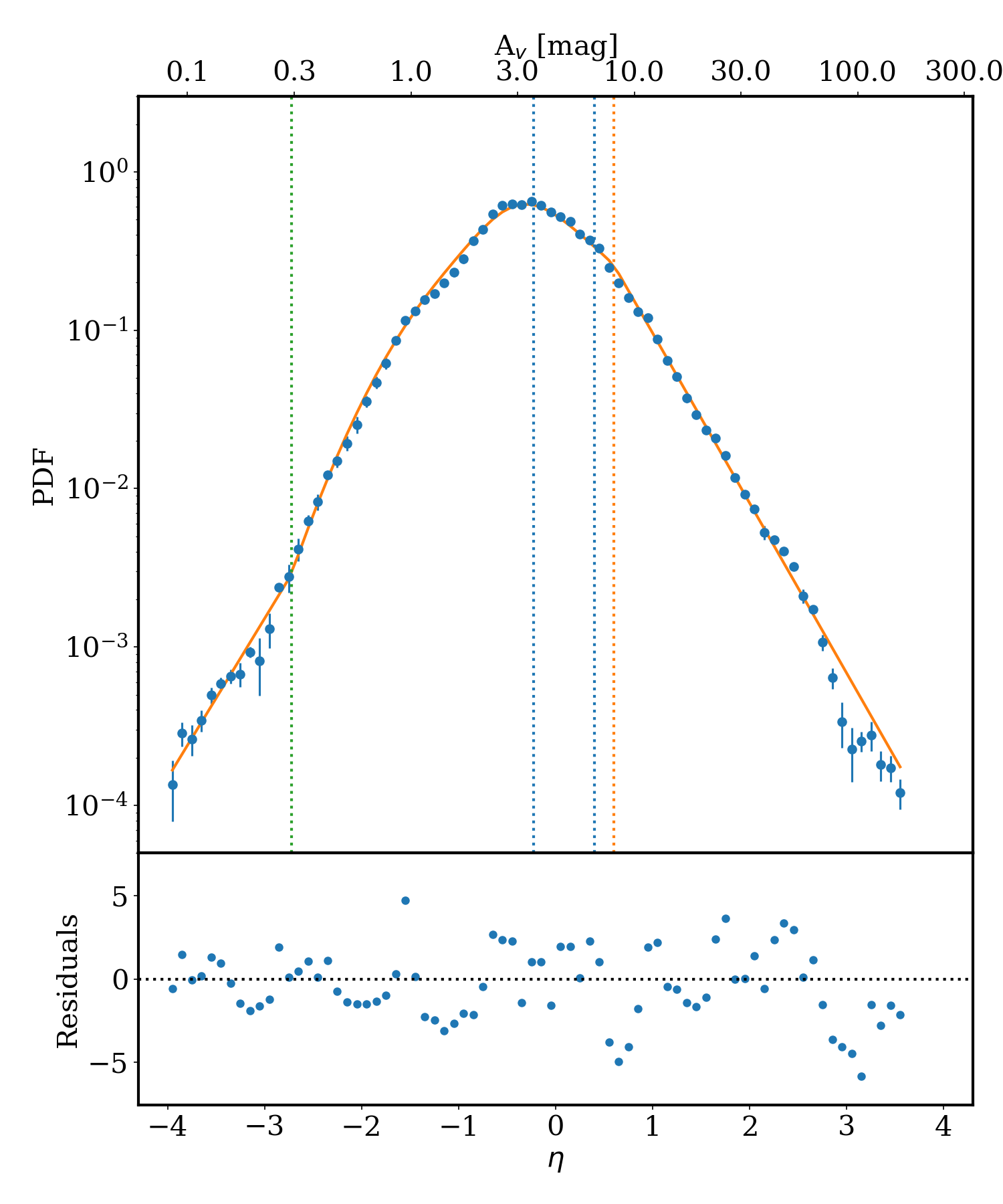
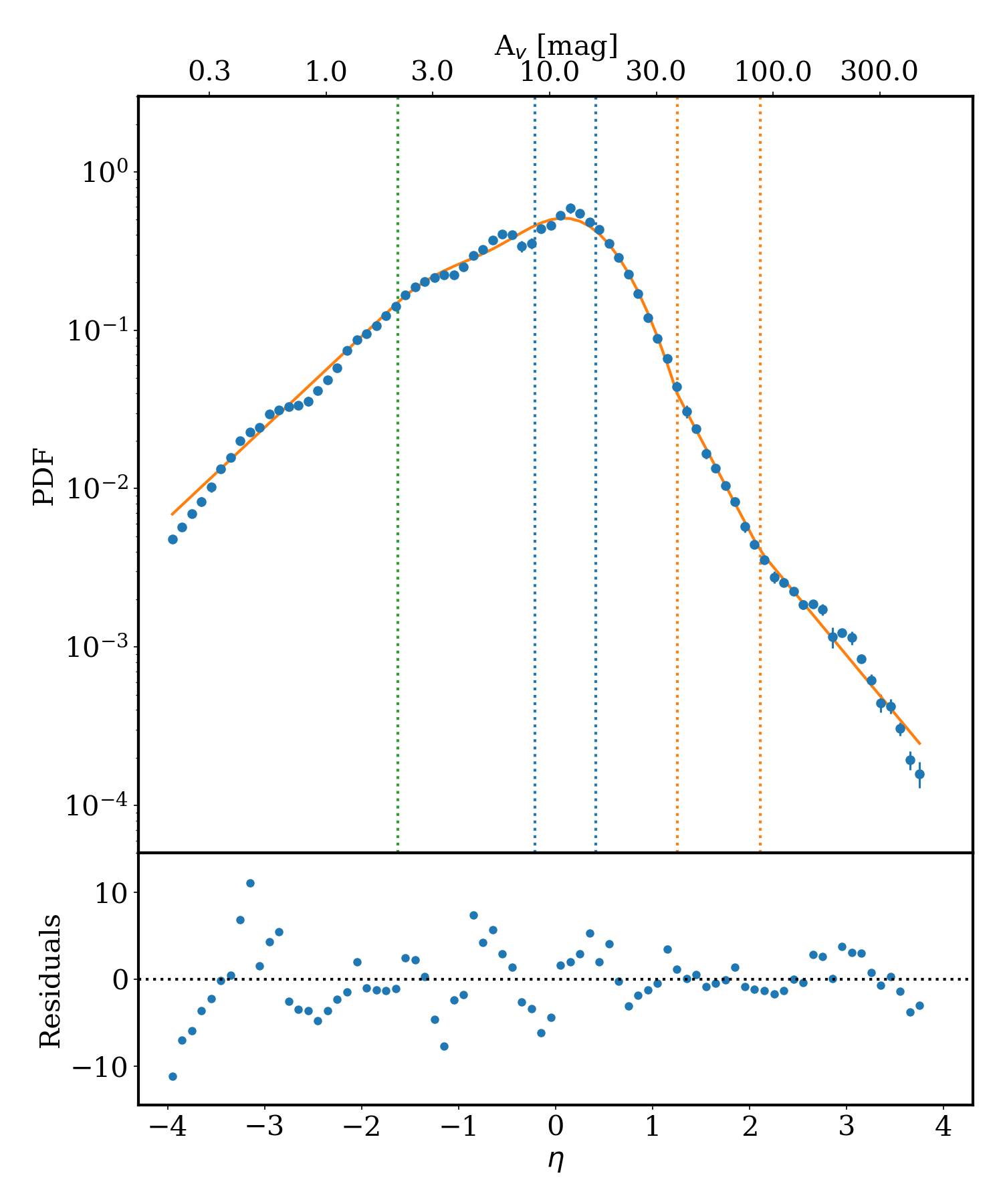
Figure 38: M16 (left) and M17 (right).

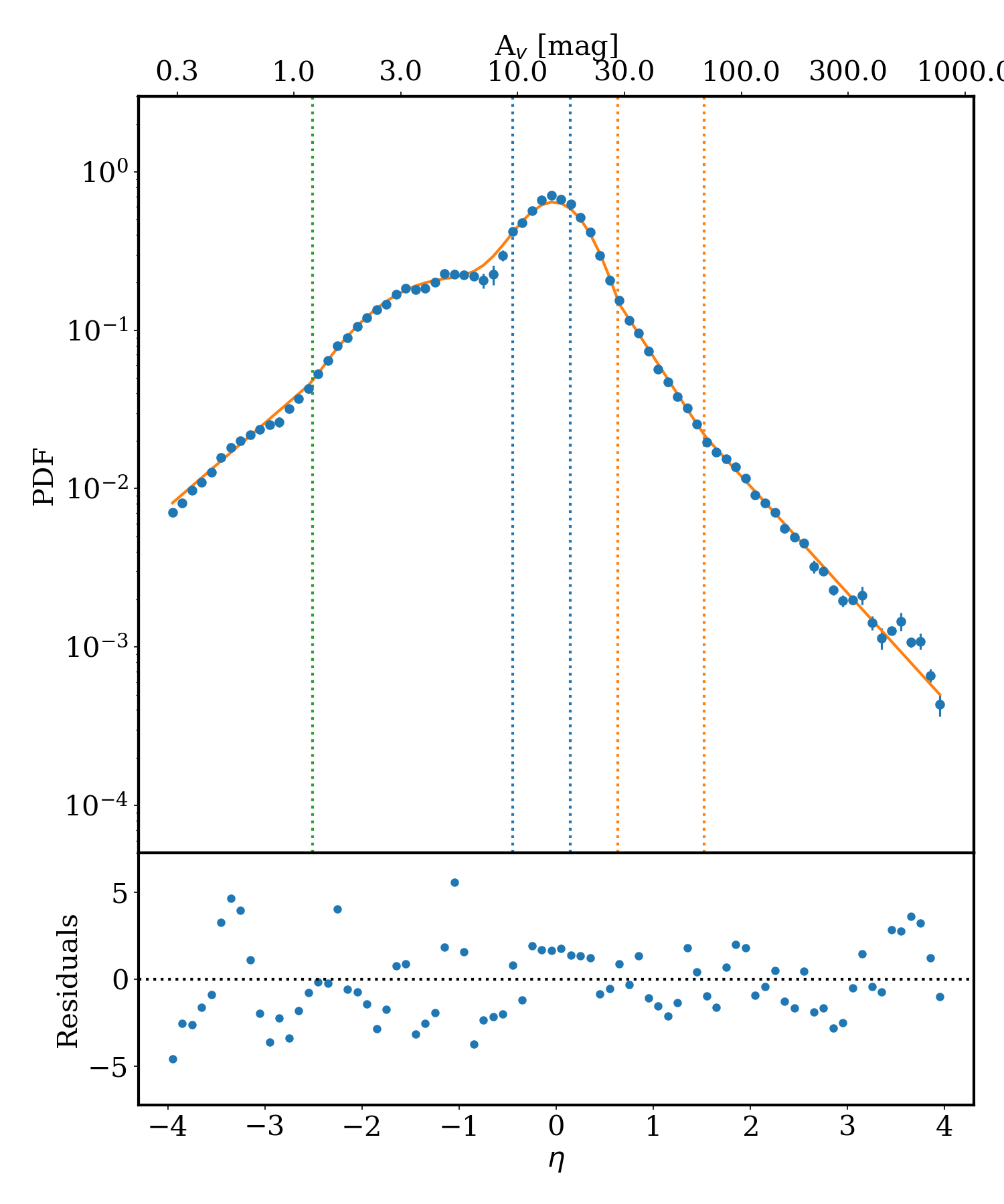
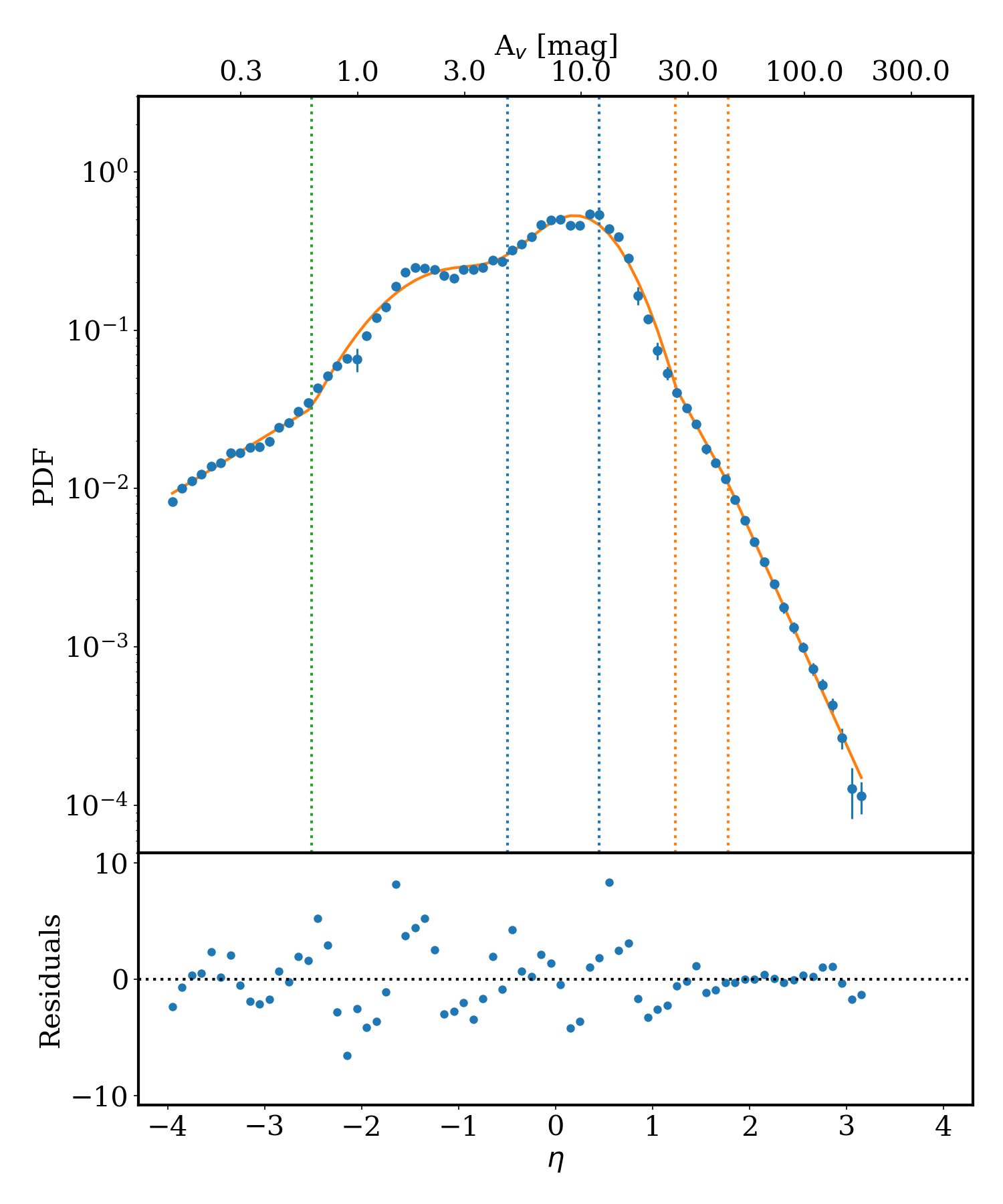
Figure 39: NGC6334 (left) and NGC6357 (right).

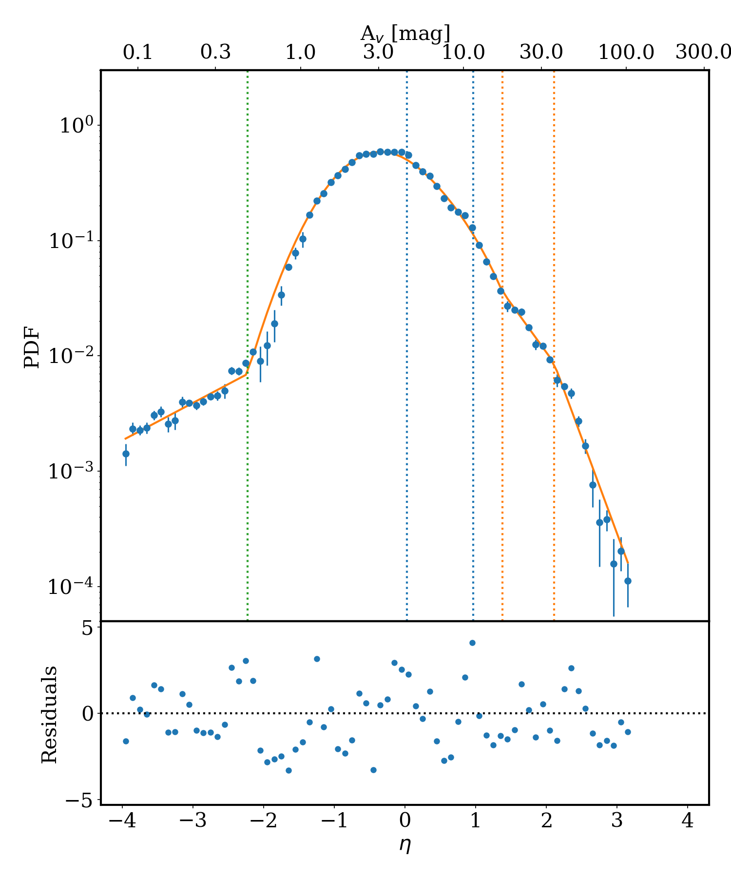
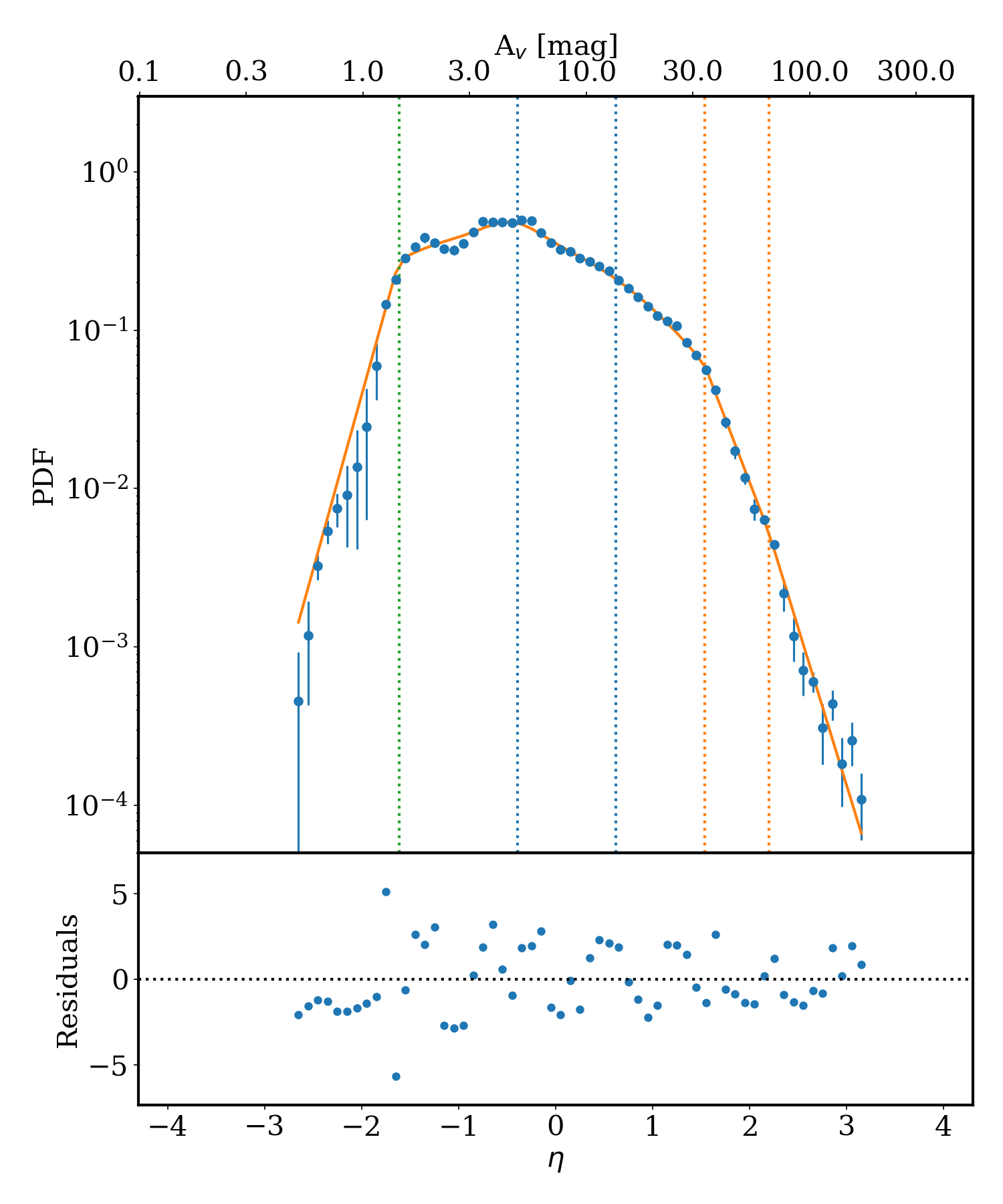
Figure 40: Rosette (left) and Vela (right).

Figure 1, Figs. 8-16 in Appendix C, and Figs. 37-40 in Appendix D display the LOS-contamination corrected column density maps and N-PDFs of massive clouds. For all clouds except of M16, the best fitting model was the one of two log-normals and two PLTs.

Log-normal distribution(s)
The peaks of the first and second log-normal are at A_V=3.0 and A_V=3.8 (median values), respectively, and the corresponding widths are $\sigma_{\rm\eta 1}$ = $\sigma_{\rm\eta 2}$ = 0.52. A double peak or a broadening of the N-PDF (see also Sec. 3.2.3) is frequently observed in regions with stellar feedback. For Rosette, NGC6334, and M16, we confirm with our high-resolution maps what was found using Herschel low-resolution maps (Schneider et al., 2012; Russeil et al., 2013; Tremblin et al., 2014). In addition, these types of N-PDFs were reported for W3 (Rivera-Ingraham et al., 2013), RCW36, and RCW120 (Tremblin et al., 2014). The second, higher column density peak is interpreted as a gas layer compressed by an expanding H II-region (Schneider et al., 2012; Tremblin et al., 2014). As shown in hydrodynamic simulations including radiation (Tremblin et al., 2012a, b, 2014), the presence of a double-peak in the N-PDF depends on the turbulent state of the cloud, it is only visible at low Mach numbers and when the cloud is dominated by ionized-gas pressure. Therefore, the double-peak is not a general feature of regions with stellar feedback.

Power law tail(s)
From the nine clouds in our sample, only one (M16) shows a single PLT, all others have two PLTs from which three sources have a flatter second slope and five a steeper one. The LOS correction has a strong influence on the first slope, making it flatter than in the original N-PDF (see Figures 8-16), but has nearly no impact on the second PLT. The resulting slope(s) of the PLT(s) vary between -1.4 and -3.7 for the first PLT, with a median of -2.37, and between -1.4 and -4.6 for the second PLT, with a median of -2.33. The higher statistics compared to Schneider et al. (2015c) shows that there is no systematic trend for high-mass SF regions that the second PLT is flatter than the first one. Both PLT slopes are thus consistent with that anticipated for the gravitational collapse of an isothermal spherical density ($\rho$) distribution of equivalent radius $R$ (Larson, 1969; Penston, 1969; Shu, 1977; Whitworth & Summers, 1985; Foster &Chevalier, 1993) with $\rho\propto r^{-\alpha}$ and $\alpha$=2. The exponent $\alpha$ and the slope $s$ are linked via $\alpha$=($-2/{\rm s}$)+1 (Federrath & Klessen, 2013; Girichidis et al., 2014; Veltchev et al., 2019).

Deviation point(s) and structure
The DP from the log-normal part to the first PLT (DP1) and the DP from the first to the second PLT (DP2) show a very large spread, with A_V(DP1)$\sim$8-37 and A_V(DP2)$\sim$19-88, respectively. The high value of DP1 is partly due to the fact that the LOS correction may still underestimate the emission along the LOS and that the maps are not extended enough. The regions characterized by high column densities (above DP2) are outlined in the plots of Appendix C with a black contour. Interestingly, there is a direct link to the $\Delta$-variance spectra that are shown in the lower right panels of Appendix C, including the values of the $\beta$-exponent(s). First, we observe that the largest variation in structure occurs at small scales because the exponent $\beta_{1}$ is small, typically between 2.0 and 2.5, with a median of 2.3 (Table 3). Second, the extent of the area defined in the column density map by the contour at DP2 corresponds approximately to the peak or turnover point of the $\Delta$-variance spectrum. For example, DP2 for M17 lies at A_V=88 and the northern clump outlined in the column density map by the black contour at that value has a linear scale of $\sim$2-3 pc and the peak of the $\Delta$-variance spectrum lies at 2.57 pc (Table 3). On the other hand, the prominent peak in the $\Delta$-variance spectrum for NGC7538 ($\beta_{1}$=2.93) occurs at $\sim$2-3 pc, which translates into a physical size of the structure of 1.2-1.8 pc. This characteristic size can either be caused by the dominating bubble in this source (at offset 15^′,10^′ in Fig. 14) or by the high-density clumps in the southeast of the map. Summarizing, the $\Delta$-variance thus points toward a scenario where the structure in massive clouds is dominated by sub-parsec scale clumps and not long filaments or ridges (Dib et al., 2020). From the column density maps, it is obvious that these clumps are located inside the most massive regions, preferentially where several filaments merge (Myers, 2011; Schneider et al., 2012).

3.2.3 N-PDFs of intermediate-mass star forming clouds

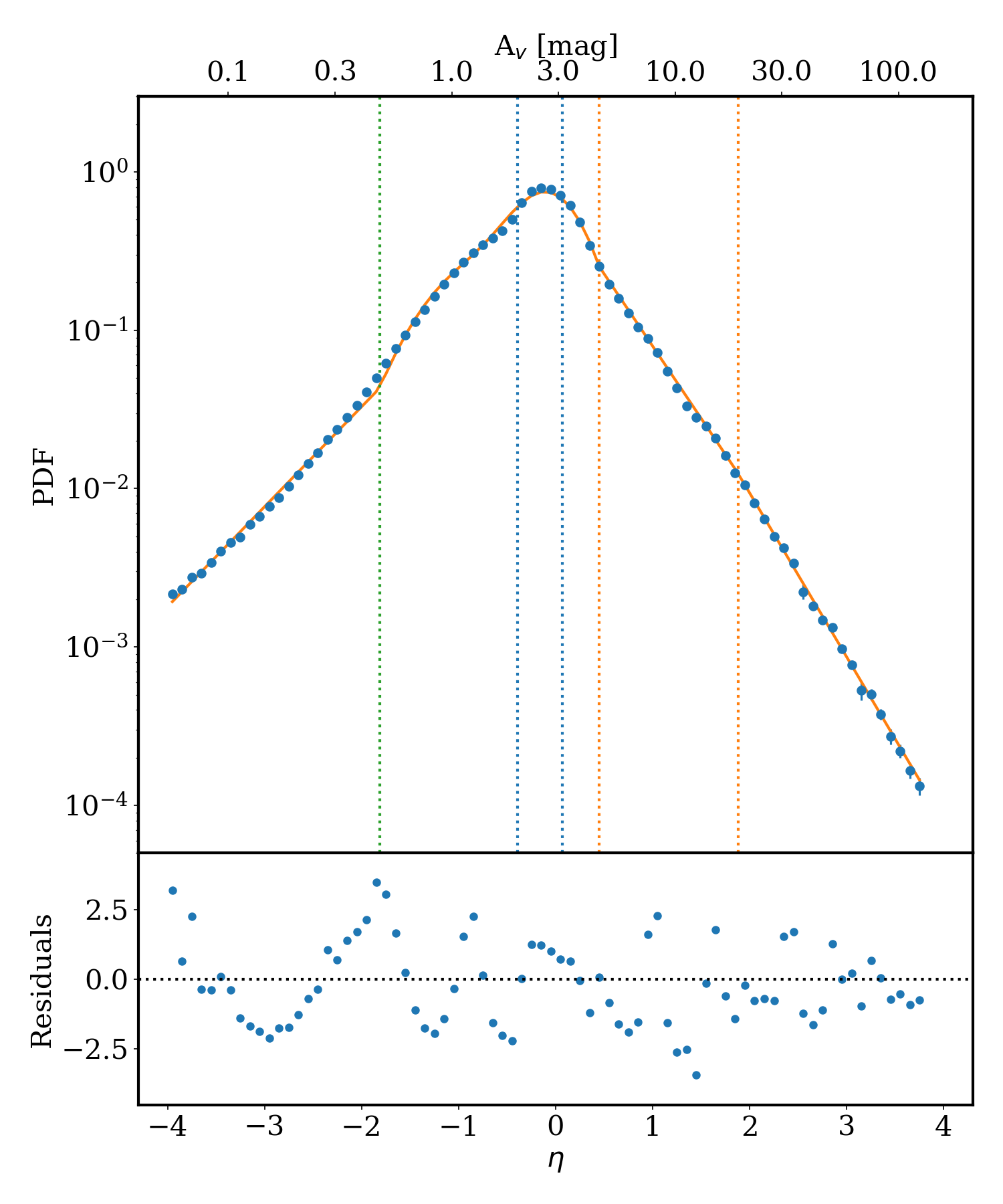
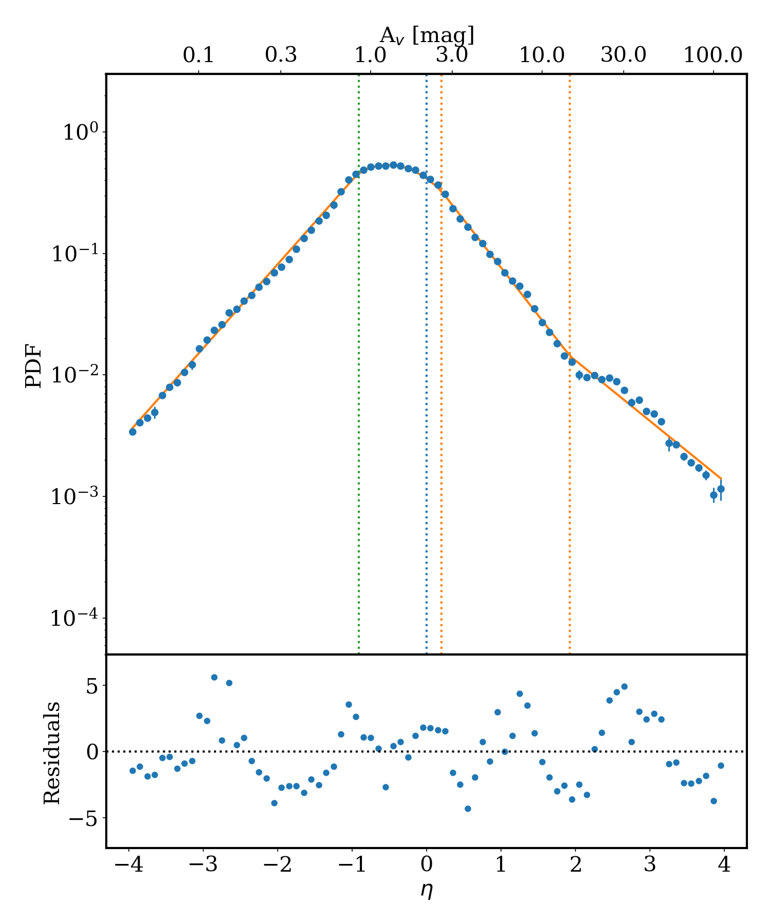
Figure 41: Aquila (left) and Mon R2 (right).

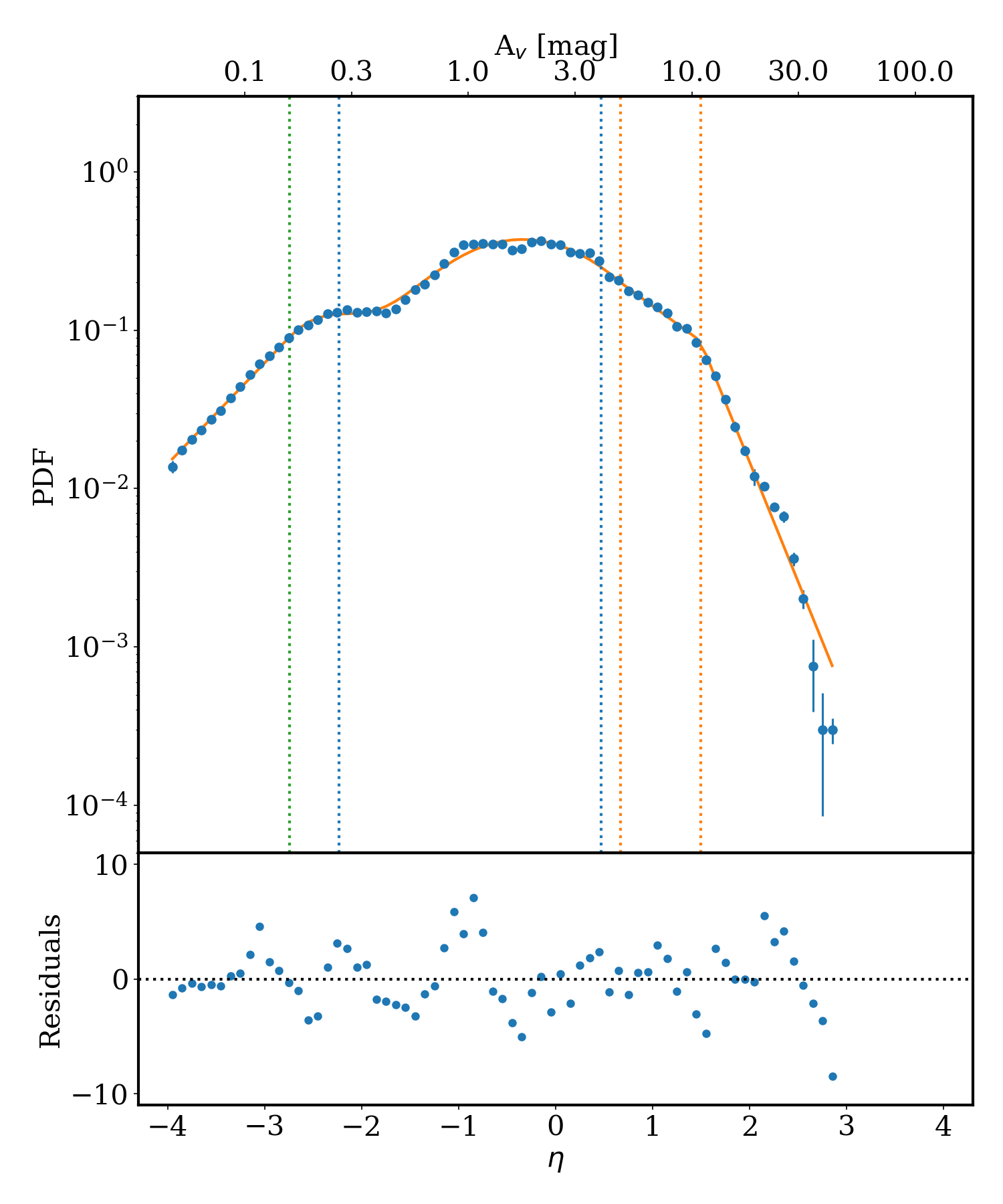
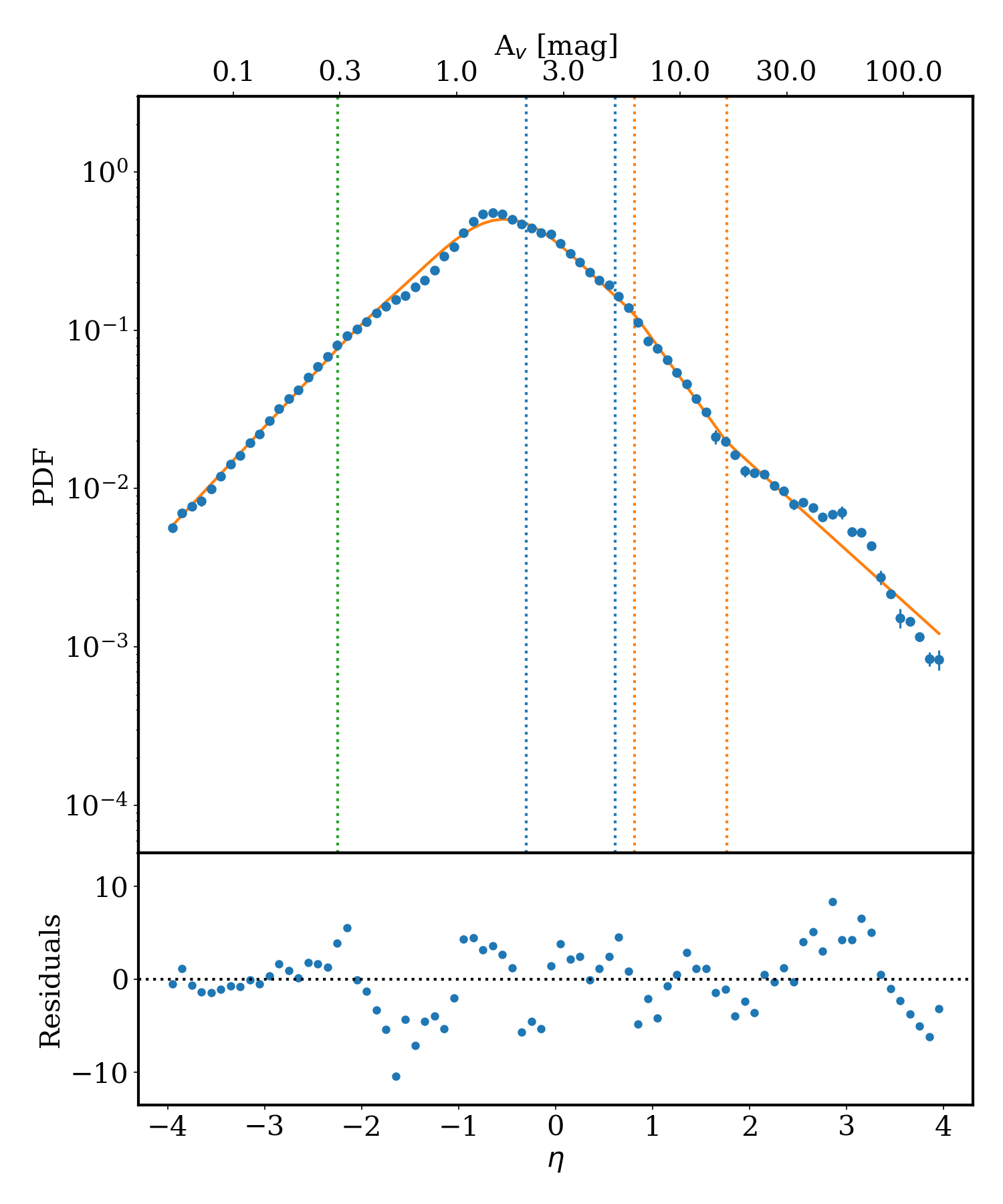
Figure 42: MonOB1 (left) and NGC2264 (right).

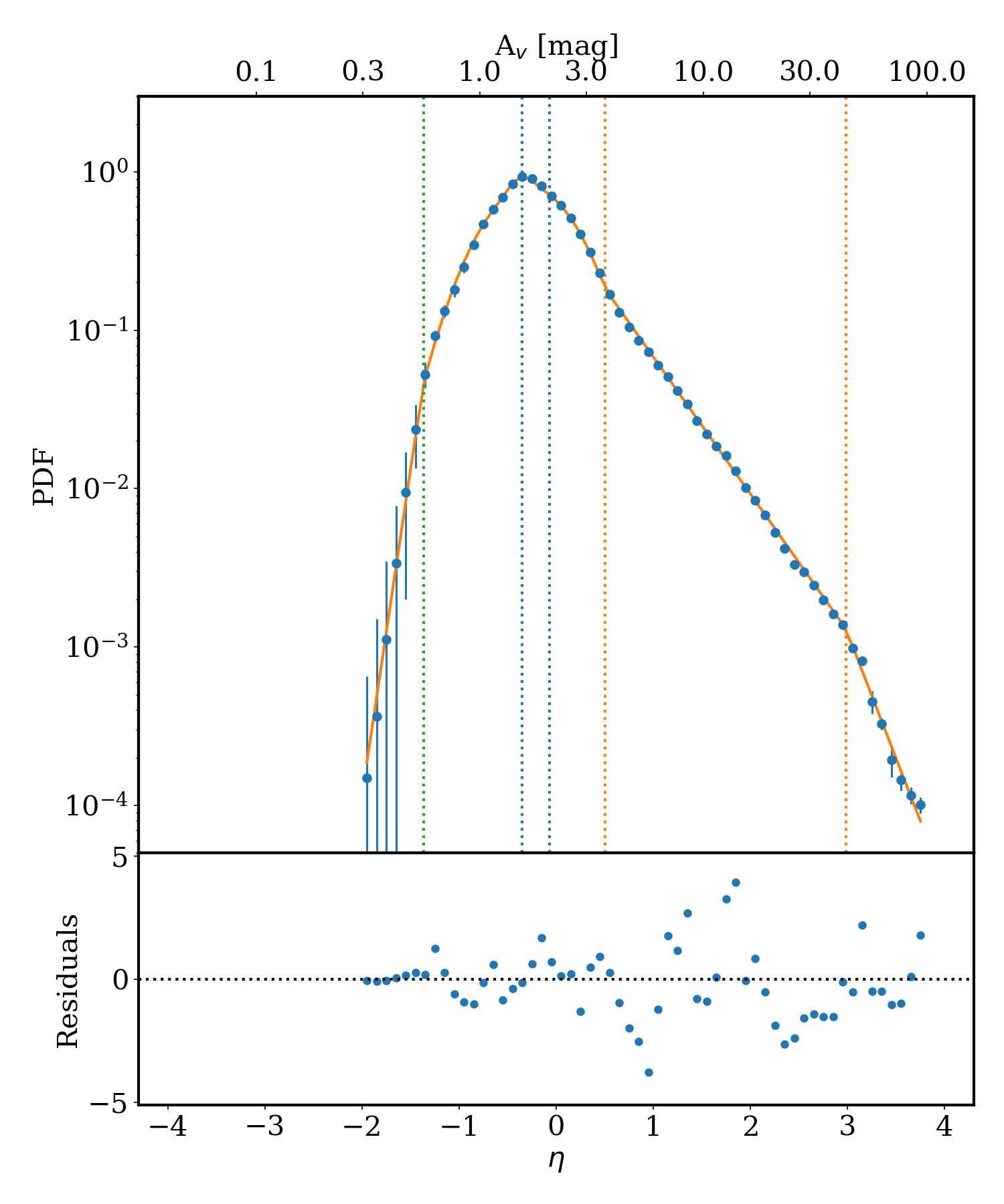
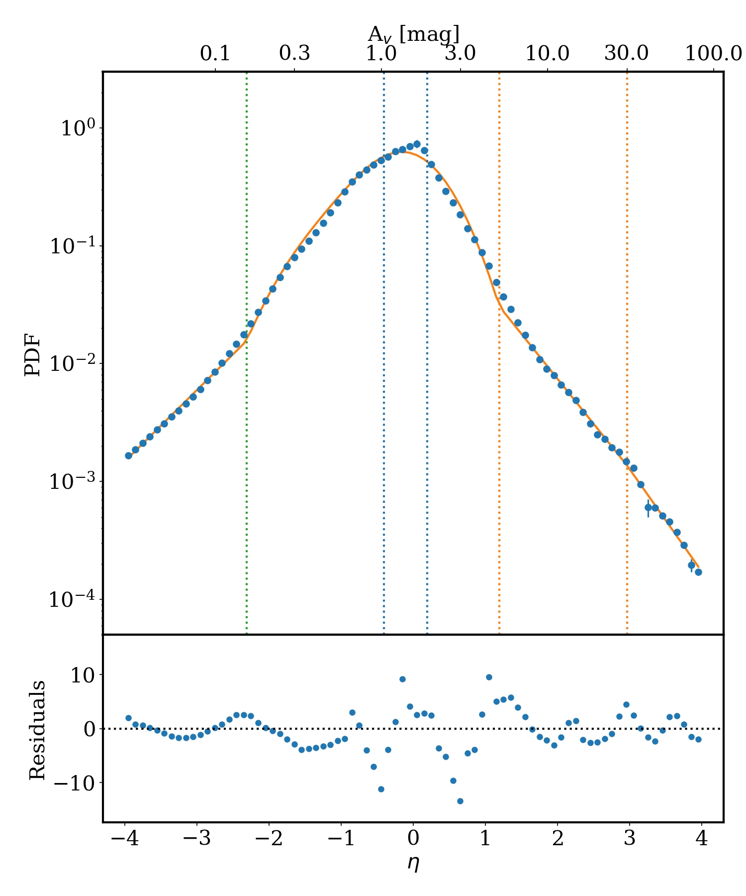
Figure 43: Orion B (left) and Serpens (right).

The N-PDFs for intermediate-mass SF regions (Fig. 1, Figs. 17-22 in Appendix C and Figs. 41-43 in Appendix D) show a very complex shape (in particular MonOB1, Vela, and NGC2264), similar to that of high-mass SF clouds.

Log-normal distribution(s)
The peaks of the first and second log-normal are at A_V=1.10 and A_V=1.68 (median values), respectively, and the corresponding widths are $\sigma_{\rm\eta 1}$ = 0.47 and $\sigma_{\rm\eta 2}$ = 0.52. The N-PDFs of Mon OB1 and NGC2264 are broader than the others, which can be explained by external compression. As shown in Schneider et al. (2013), and conforming with numerical models (Tremblin et al., 2012a, b), external compression mainly due to radiative effects caused by close-by H II -regions leads to a broadening of the N-PDF. Observationally, this influence becomes also obvious in cuts of column density profiles (Peretto et al., 2012; Schneider et al., 2013; Tremblin et al., 2013).

Power law tail(s)
All clouds in the sample have two PLTs from which only two regions (MonR2, NGC2264) have a flatter second slope. For the first PLT, typical values for the slope scatter around -2 (the median is $s_{1}$=-1.88). For the second PLT, the variation is large, the median of all sources is $s_{2}$=-2.19. These values are again consistent with what is expected for gravitational collapse.

Deviation point(s) and structure
The first DP shows a small scatter with a median of 4.7, while DP2 varies more, with a median of 17.7.
There seems to be no clear correlation between cloud morphology and N-PDF shape. The two sources with the clearest flatter second PLT are MonR2 with a dominant hub-filament geometry and NGC2264 with a dominant ridge structure. And the two sources with a steeper second PLT are MonOB1, which is basically a large clump, and Vela C, which has also a dominant ridge structure. The morphology for the areas constituting the densest gas (above DP2), however, is always clumpy, over scales from sub-parsec sizes up to a few parsecs.

The $\Delta$-variance spectra are more complex than those for high-mass SF regions. We typically observe an increase in structure until a first peak (or turnover into a flat spectrum) around 0.3 pc to 1.8 pc (Table 3) with a median value of $\beta_{1}$=2.32, followed by a second increase of the spectrum with a median $\beta_{2}$=2.56 and a peak around 4 pc. Similar to high-mass SF regions, small $\beta$ values indicate the largest structure variation on small scales. These are then possibly the sub-parsec- to parsec-scale dense clumps, filaments and cores that are embedded in the molecular cloud. The questions arises how the $\Delta$-variance spectrum now links to the N-PDF. One correlation is seen in MonR2. The dense, central clump, in which a whole cluster is forming, has a size scale of around 1-2 pc (Fig. 18), which is also the size derived from the peak in MonR2’s $\Delta$-variance spectrum (peak at $\sim$2 pc, corresponding to a size of 1.2 pc). The N-PDF, on the other hand, shows a slope change (from a steep into a flat PLT) at an A_V around 15. This level of emission corresponds in the column density map (left panel in Fig 18) exactly to the central clump, visible where the color changes from green to yellow. Another good example is Mon OB1 (Fig 19), where the N-PDF PLT slope change occurs at A_V$\sim$10, which corresponds to regions with a size scale of around 1 pc.

3.2.4 N-PDFs of low-mass regions

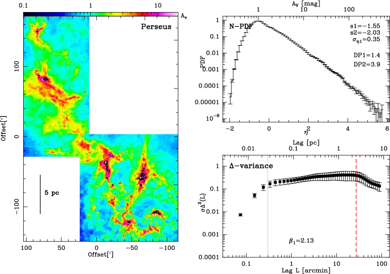
Figure 29: PERSEUS: Fig. caption see Fig. C.1.

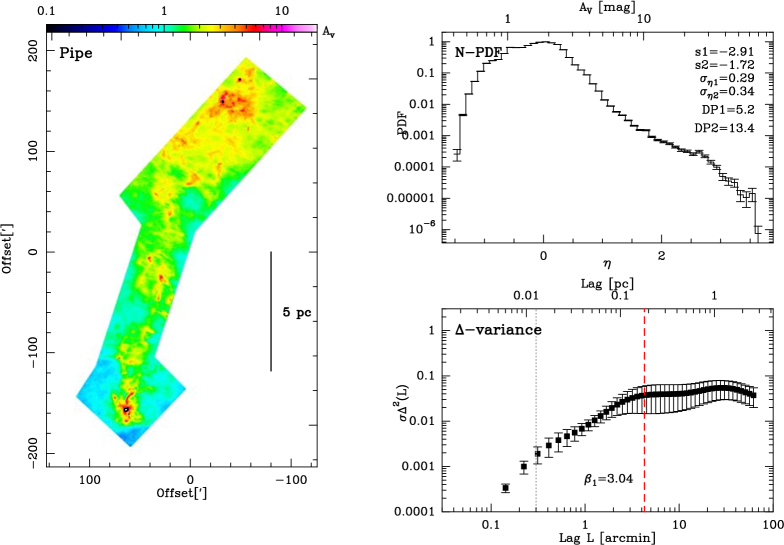
Figure 30: PIPE: Fig. caption see Fig. C.1.

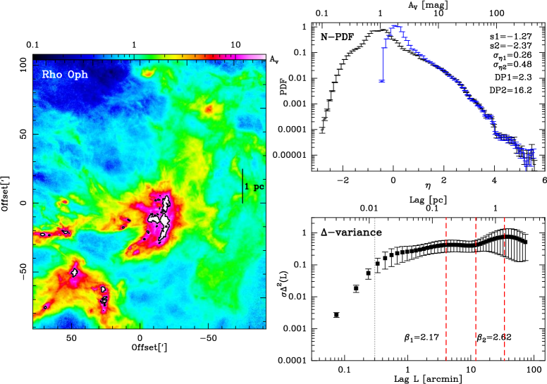
Figure 31: RHO OPH: Fig. caption see Fig. C.1. For comparison, the N-PDF of the uncorrected map is displayed in grey.

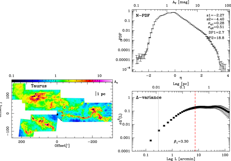
Figure 32: TAURUS: Fig. caption see Fig. C.1.

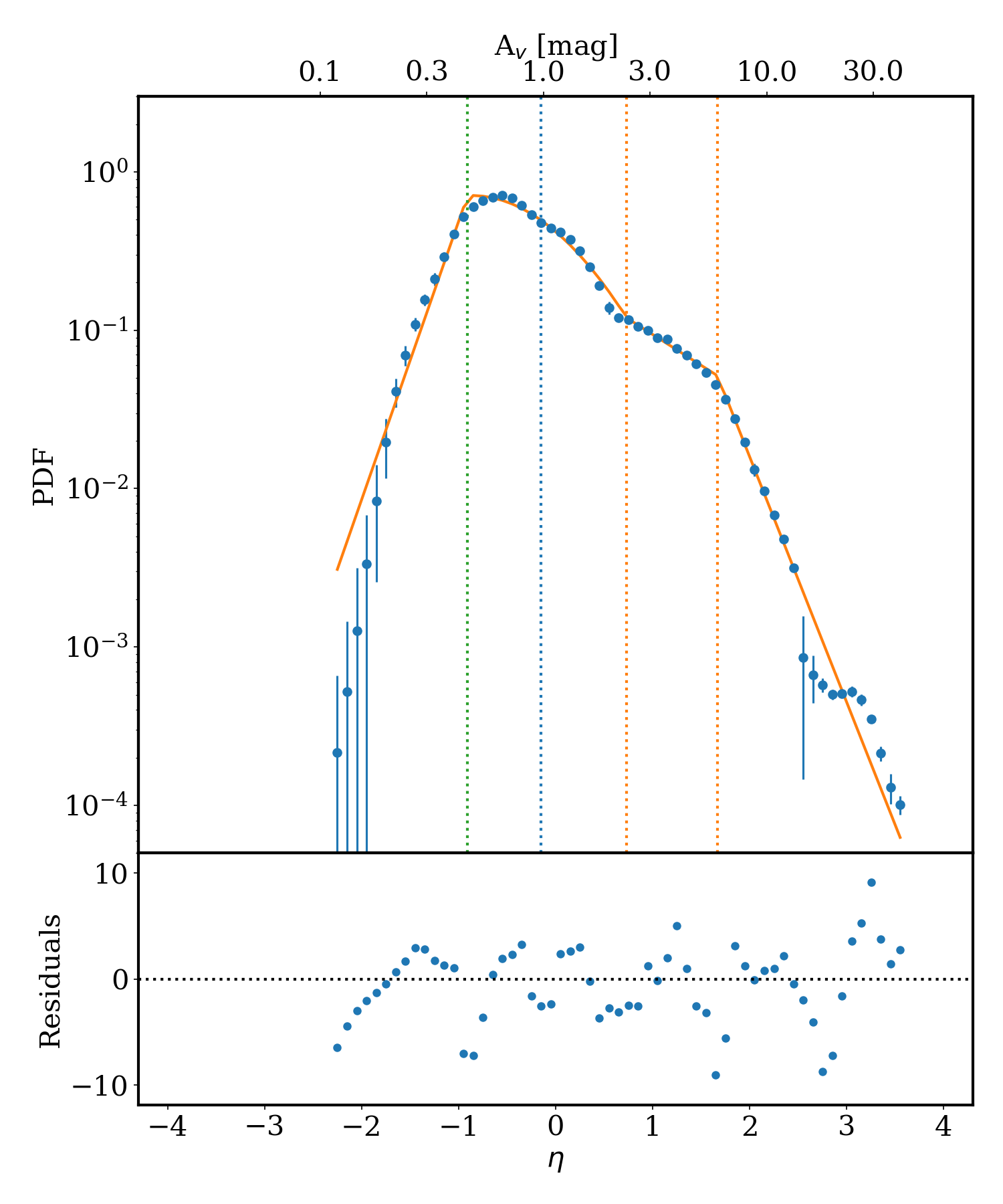
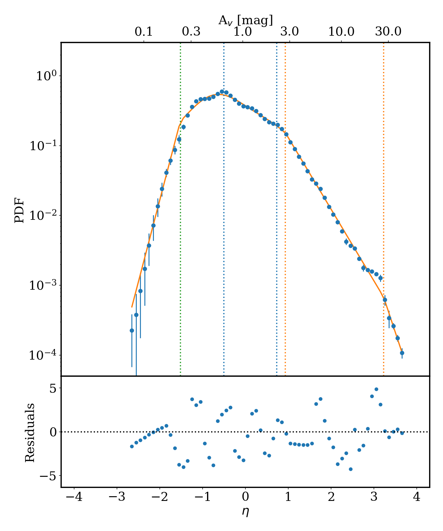
Figure 44: ChamI (left) and ChamII (right).

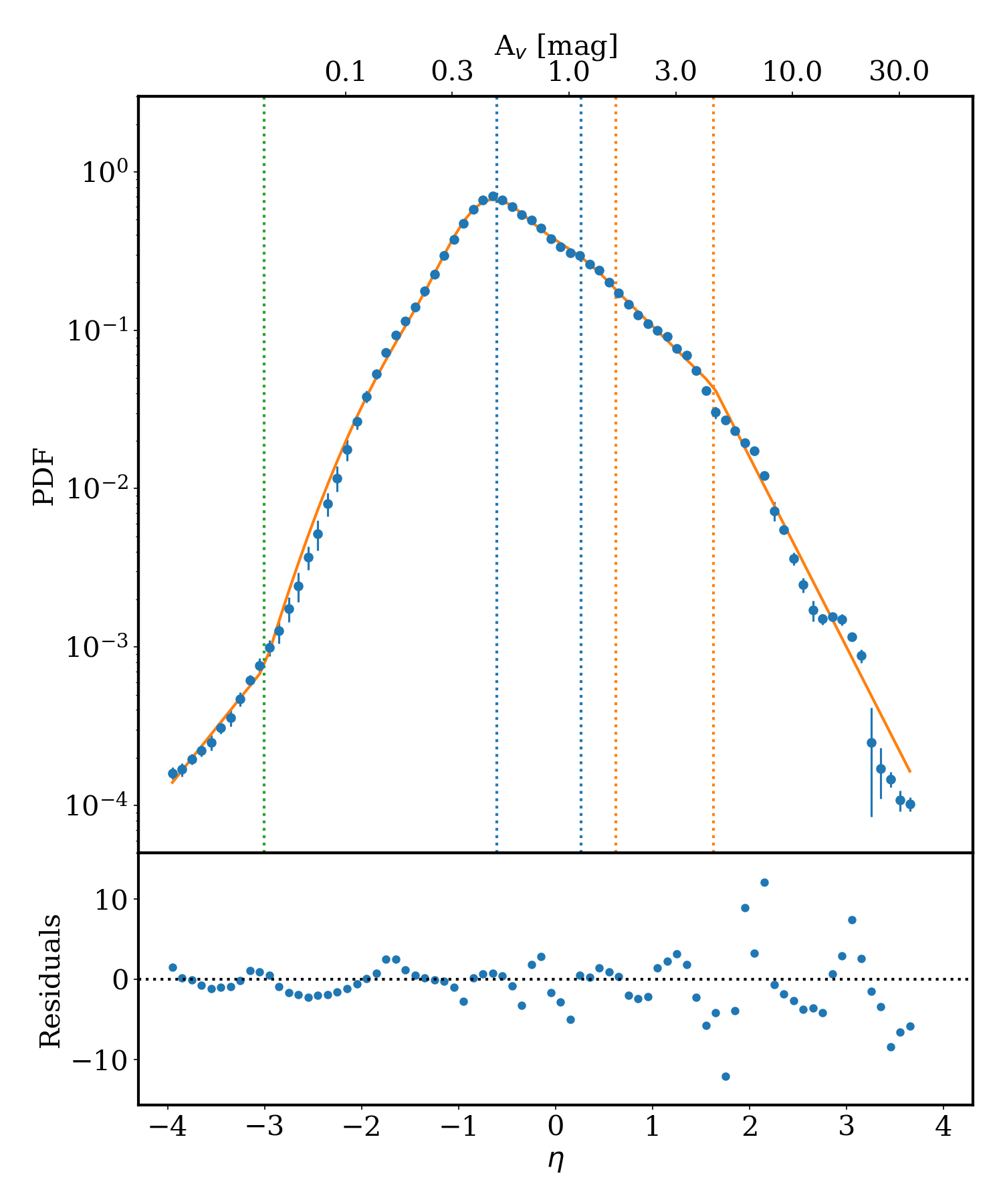
Figure 45: IC5146 (left) and Lupus I (right).

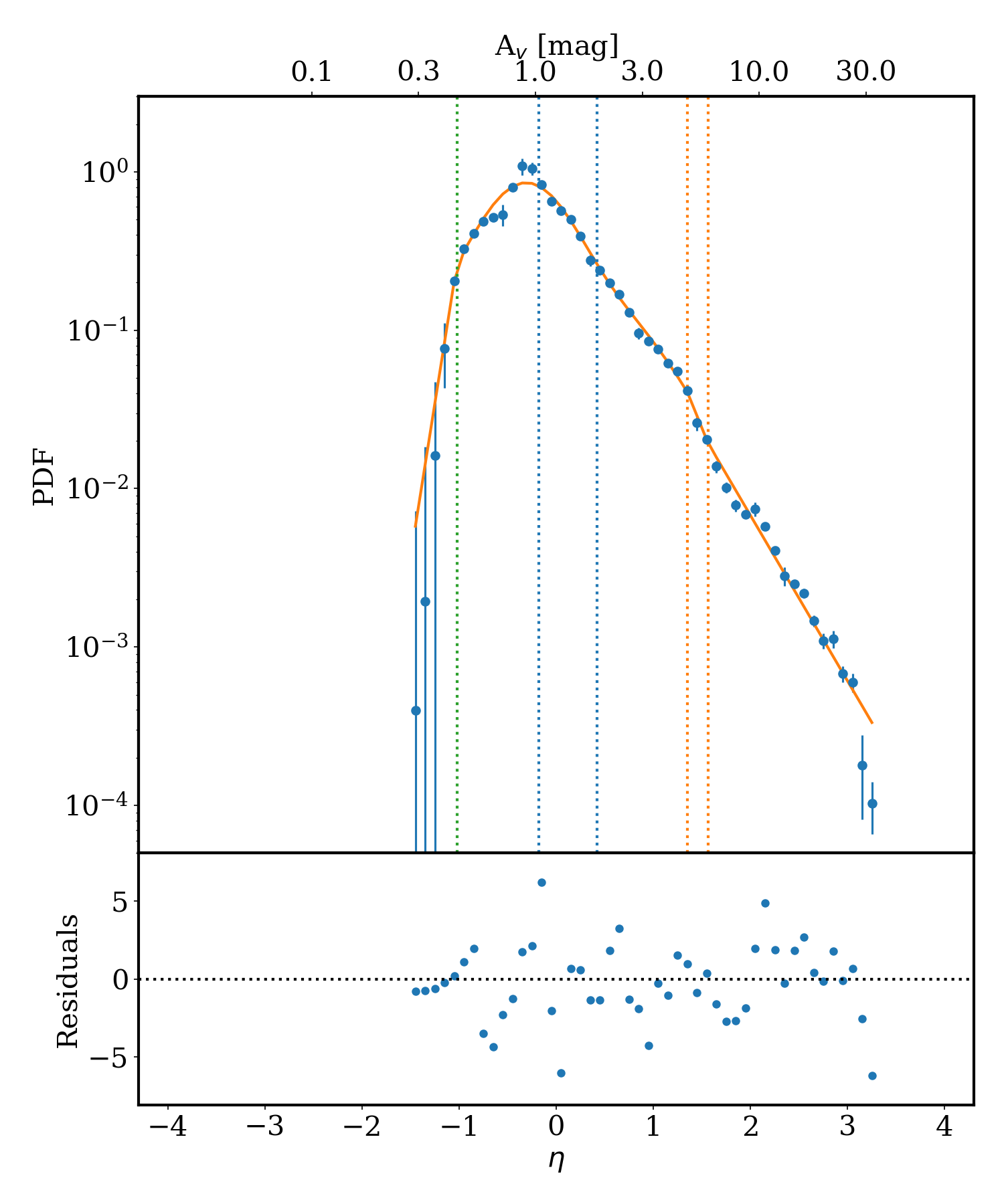
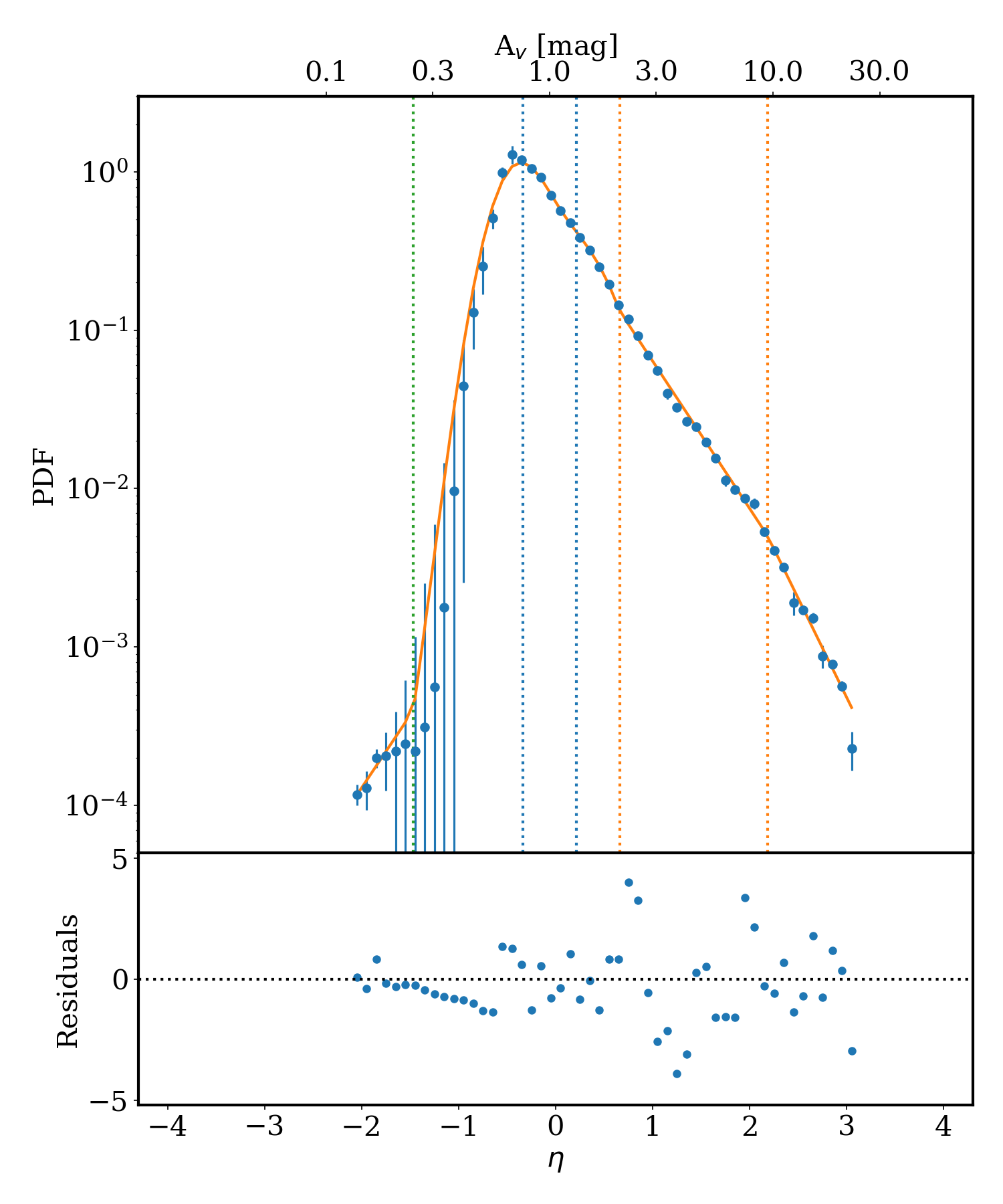
Figure 46: Lupus III (left) and Lupus IV (right).

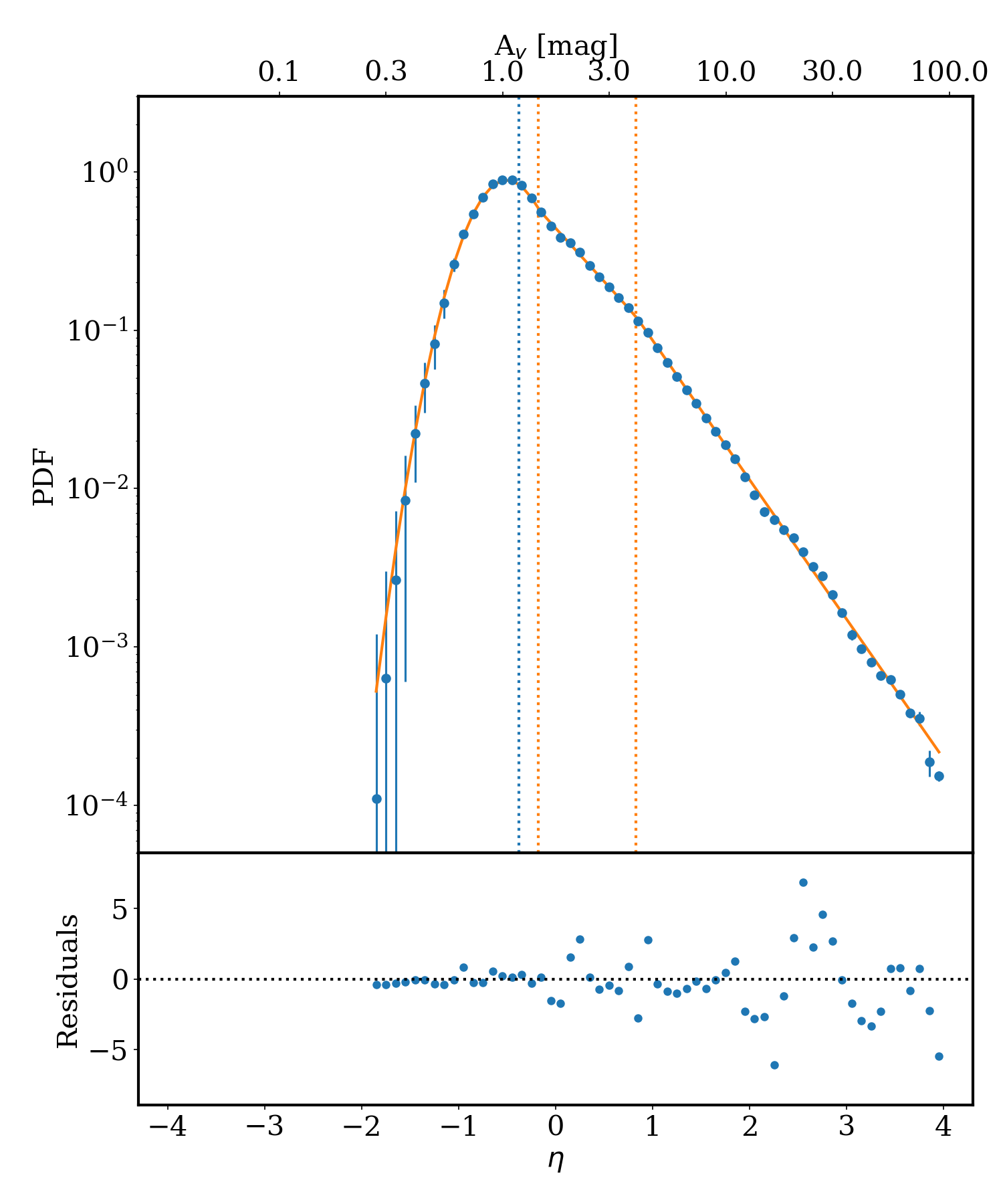
Figure 47: Perseus (left) and Pipe (right).

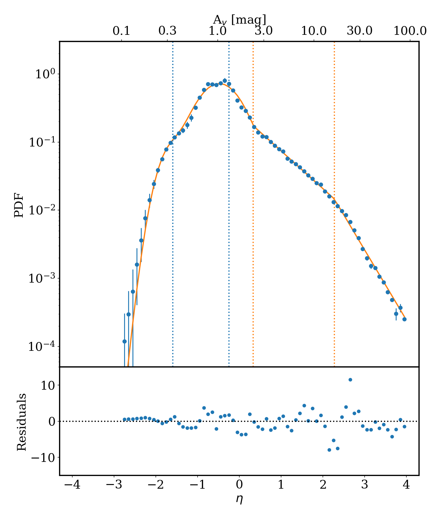
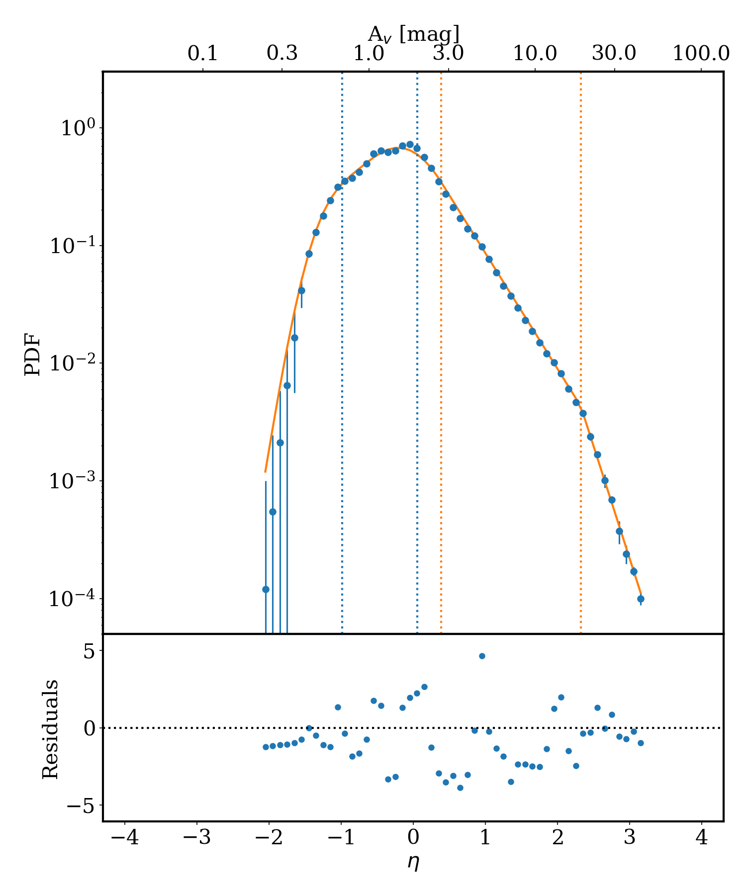
Figure 48: Rhooph (left) and Taurus (right).

The N-PDFs of low-mass star-forming regions are displayed in Fig. 1, Figs. 23-32 in Appendix C and Figs. 44-48 in Appendix D. There are some clouds that have N-PDFs with a well-defined shape, defined by a rather clear log-normal part at lower column densities and a PLT at higher column densities (IC5146, Lupus III, Lupus IV, Perseus, $\rho$Oph, Taurus). Others, however, exhibit N-PDFs with a bumpier shape (Cham I, Cham II, Cham III, Lupus I, Pipe).

Log-normal distribution(s)
All clouds except of Perseus are best fitted with two log-normals of which the first one has values between A_V=0.3 and 1 for the first peak (the median is A_V= 0.7) and the second one a median A_V of $\sim$1. The widths of the log-normals are $\sigma_{\rm\eta 1}$ = 0.32 and $\sigma_{\rm\eta 2}$ = 0.64. In contrast to high-mass SF regions, where the two log-normals can both be attributed to purely molecular gas and the second bump to the effect of stellar feedback, we are here in a regime where there can be a contribution from atomic hydrogen (Mandal et al., 2022). The peak of the first log-normal N-PDF always lies below A_V = 1 (in most of the cases significantly lower, only Perseus and Pipe have a value of A${}_{\rm V,pk1}\sim$1). The H I-to-H₂ transition depends on many parameters such as the external radiation field, the density, and turbulence, and is predicted to happen between A_V$\sim$0.1-0.4 (Röllig al., 2007; Glover et al., 2010; Wolfire et al., 2010; Bialey et al., 2017; Bisbas et al., 2019). The extinction when CO arises from a fully molecular phase (”CO-bright H₂”) is around A${}_{\rm v}\sim$1 (Röllig al., 2007; Visser et al., 2009; Sternberg et al., 2014). We emphasize that these A_v values given in the literature are local values, expressed as A_v,3D (Seifried et al., 2020). The observational visual extinction is derived by averaging along the LOS dubbed as A_v,2D, and is a factor of a few larger (see discussion in Seifried et al. (2020). Considering this fact, it is thus reasonable that the peak of the first log-normal part of the N-PDF arises from the atomic gas. Reducing the observational median A_v,2D of 0.7 and 0.45 for low-mass and quiescent regions, respectively, by a factor of three for example, would imply a A_v,3D of 0.23 and 0.15, which is well in the range of the H I-to-H₂ transition. In Sec. 3.2.6, we discuss the N-PDFs of Draco that shows only two log-normal parts of the N-PDF, where we present additional evidence for our proposition. But the low-mass clouds we present here can be in an early evolutionary state and the atomic envelope (Imara & Burkhart, 2016) may be more prominent. The atomic and the molecular gas then have both log-normal N-PDFs (caused by turbulent mixing) that overlap (Mandal et al., 2022).

Power law tail(s)
All clouds are again fitted with two PLTs, but interestingly, the majority (8 out of 10) have a steeper second PLT compared to the first one. The median value for the first PLT is $s_{1}$ = -1.85 and for the second PLT $s_{2}$ = -2.76. This is a new feature in N-PDFs and discovered most likely thanks to the higher angular resolution of the maps. While the first PLT slope is consistent with that expected for gravitational collapse at early stages (Larson, 1969; Penston, 1969; Shu, 1977; Whitworth & Summers, 1985; Federrath & Klessen, 2013; Girichidis et al., 2014), it is unclear what could cause the steeper second PLT. It can be related to magnetic fields, which we discuss in more detail in Sect. 4.

Deviation point(s) and structure
The DP1 is overall at lower values (median A_V(DP1) = 2.5) but there is a large scatter in the values between 1.4 and 5.2.
There are interesting differences in the shapes of the $\Delta$-variance spectra. Nearly all sources (the best example, however, is Perseus) show little variation in structure (flat spectrum) between $\sim$0.3 pc and 1 pc. Below $\sim$0.3-0.5 pc (the first peak, P1 in the $\Delta$-variance spectrum, see Table 3), there is the largest structural variation where the median of the exponent $\beta_{1}$ is 2.86. Most of the sources show an increase in the $\Delta$-variance spectrum after the flat range with a second peak typically at 1-3 pc (only Lupus IV shows a peak at 6.5 pc). The median of the exponent $\beta_{2}$ is 2.64. We observe a similar correlation between the slope change of the N-PDF at DP2 and the structural change visible in the $\Delta$-variance spectrum (at scale P1) as was detected for high-mass and intermediate-mass SF regions. We, however, do not distinguish here between a change into a flatter or steeper PLT. In the clouds Cham I, Cham II, Pipe, Taurus, the extent of the higher density regions with a flatter or steeper PLT outlined by the black contour in the column density map corresponds approximately to the first characteristic scale (P1) in the $\Delta$-variance spectrum. The values of P1, however, are not always the same and there is a trend that clouds with higher DP2 show smaller values for P1. For example for Cham I, A_V(DP2)=6.0 and P1=0.21 pc while for Cham II, A_V(DP2)=26.9 and P1=0.61 pc. We come back to this point in the next section. In some sources (IC5146, Lupus I, Perseus), there is no clear correlation between DP2 and P1, or it is less obvious ($\rho$Oph). There is another trend that the sources with the flattest $\Delta$-variance spectra (such as Perseus) have the best defined single PLT. This behavior is consistent with numerical experiments where small-scale fluctuations increase as the medium becomes full of shock compressed high-density clumps and filamentary structures, which shape the high-density end of the N-PDF.

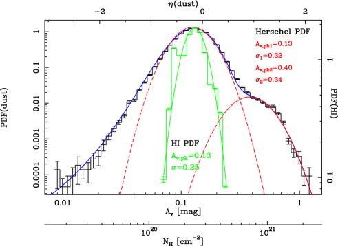
Figure 2: N-PDF of the Draco region. The black histogram shows the N-PDF obtained from Herschel data and the blue line its analytic description. The red line is the result from fitting two log-normal PDFs and considering the noise contribution that leads to a linear behavior at low column densities (Ossenkopf et al., 2016). The green histogram displays the N_HI-PDF of the H I data and the continuous line a single log-normal fit. The fitted peak positions of the PDFs and the widths ($\sigma$ in units of $\eta$=ln(N/$\langle N\rangle$)) are given in the panel. Error bars are based on Poisson statistics. The left y-axis gives the probability density for the Herschel map and the right y-axis for the H I map.

3.2.5 N-PDFs of quiescent regions

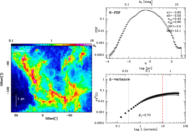
Figure 33: Chamaeleon III: Fig. caption see Fig. C.1.

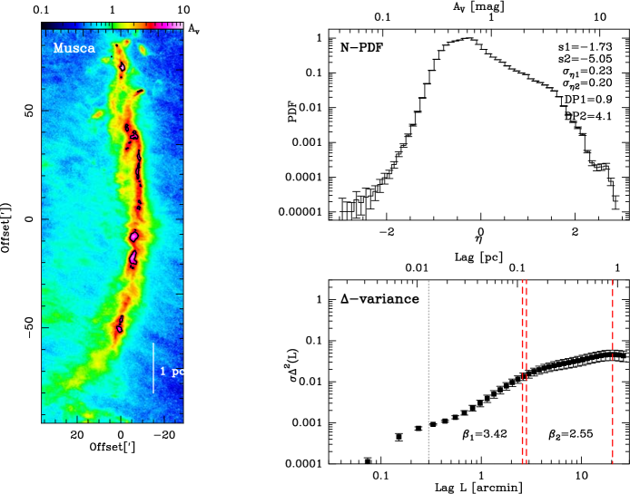
Figure 34: MUSCA: Fig. caption see Fig. C.1.

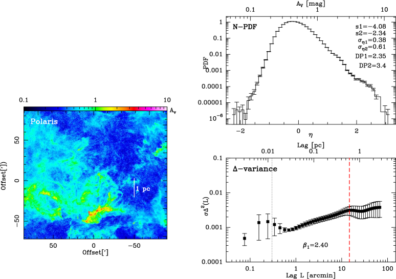
Figure 35: POLARIS: Fig. caption see Fig. C.1.

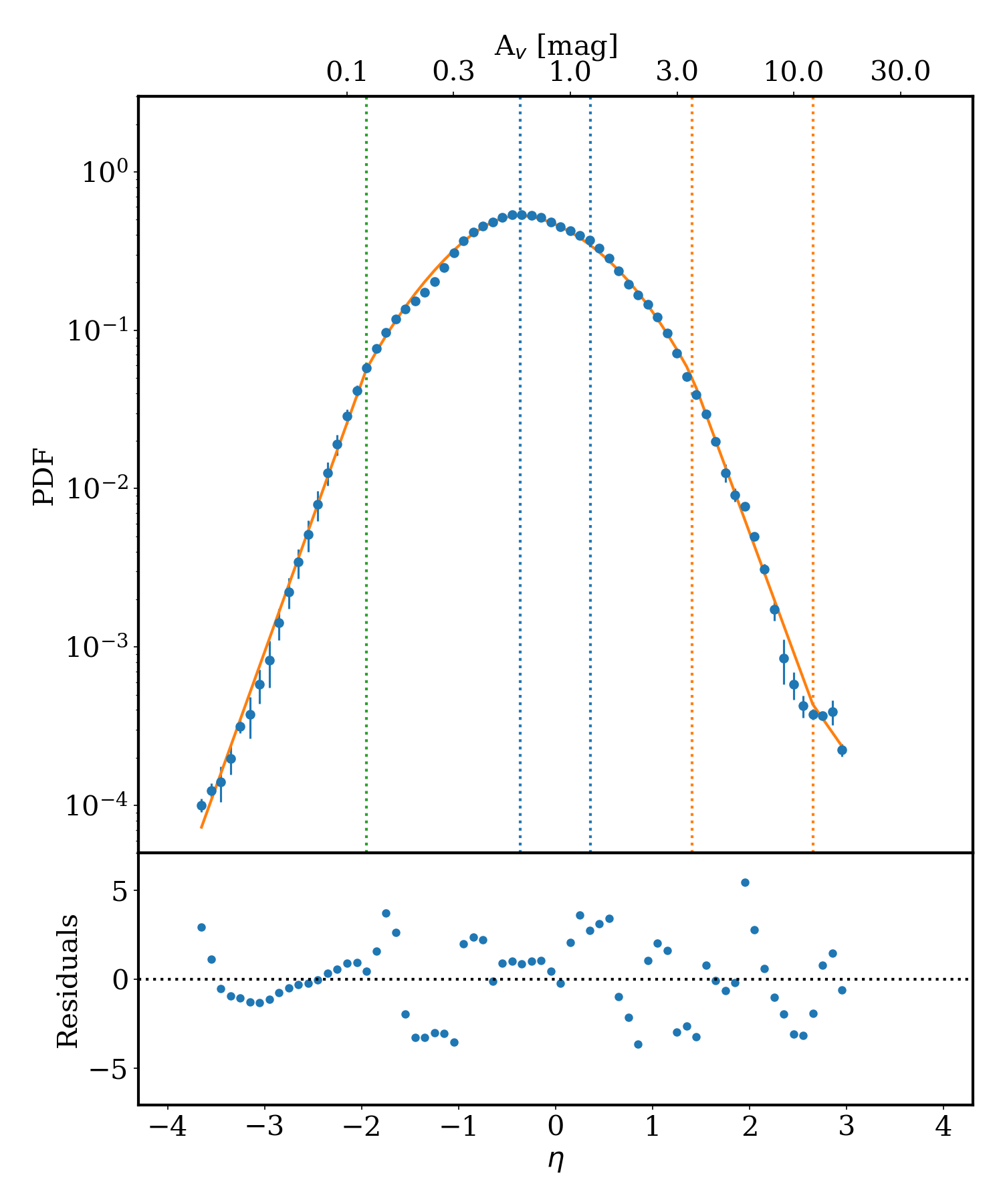
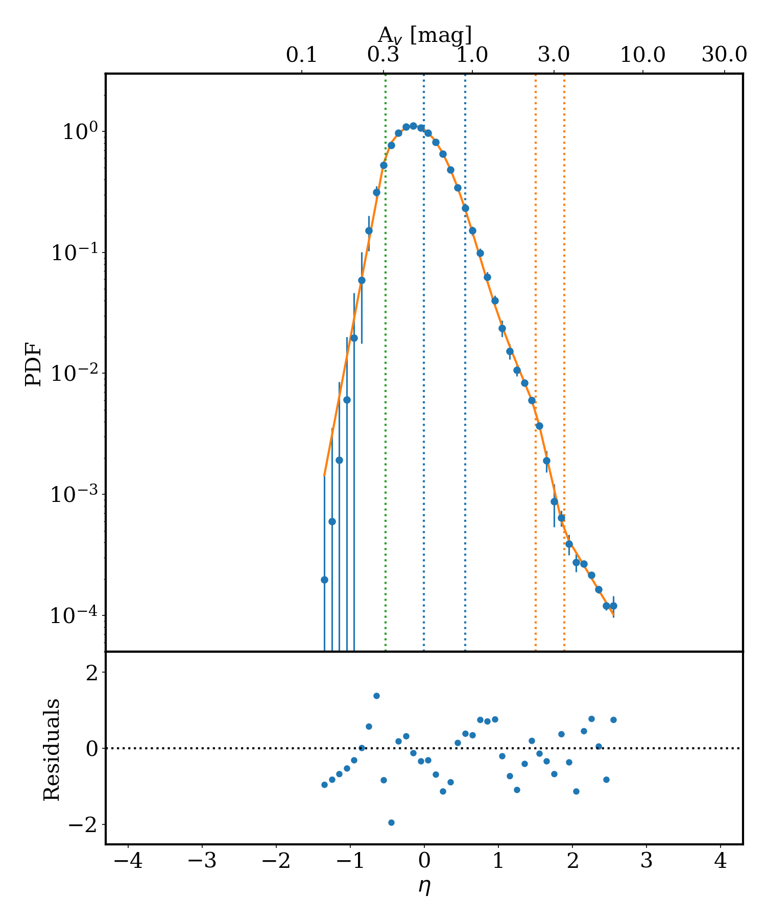
Figure 49: Cham III (left) and Polaris (right).

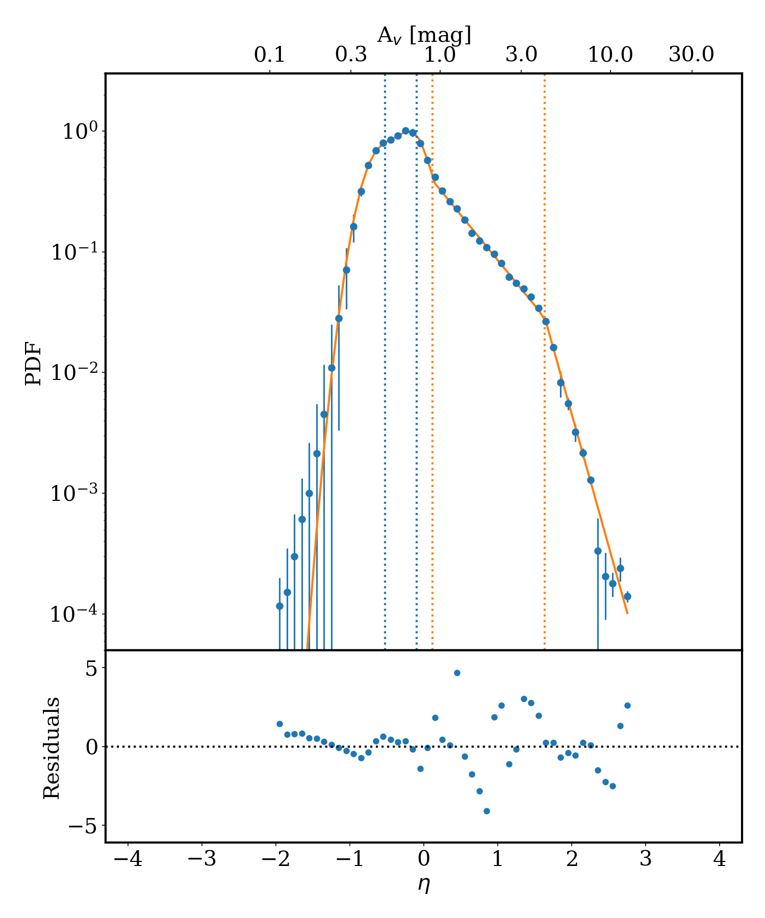
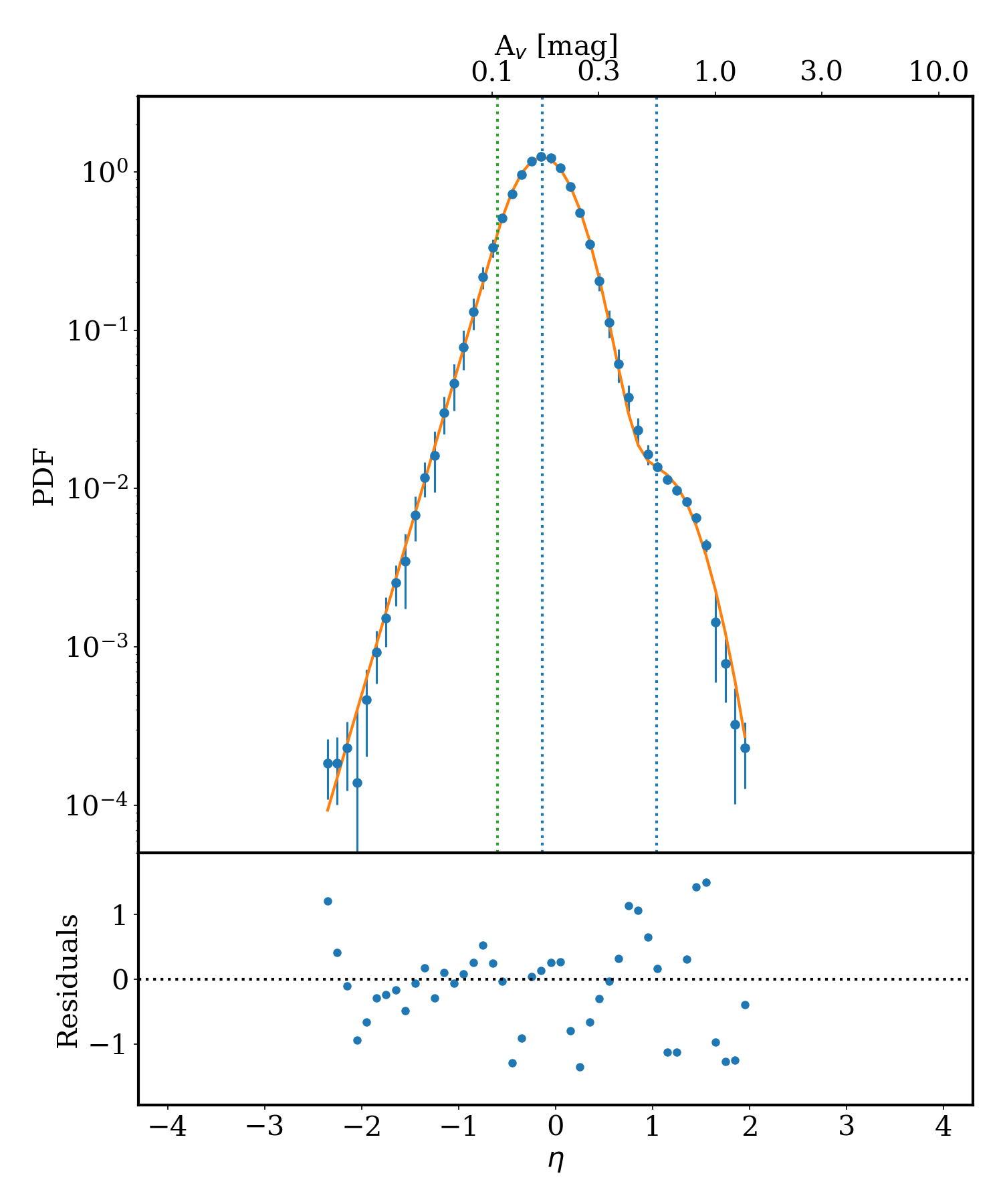
Figure 50: Musca (left) and Draco (right).

The sample we have for quiescent clouds that are not actively forming stars is small (Fig. 1). Only three clouds are included, namely Cham III (Fig. 33 and Fig. 49), Musca (Fig. 34 and Fig. 50), and Polaris (Fig. 35 and Fig. 49). All sources are fitted with two log-normals and two PLTs.

Log-normal distribution(s)
The two log-normals fitted for quiescent clouds both have their peak at low column densities (median A_V= 0.45 and A_V= 0.64, respectively) so that we here also attribute the first log-normal to a mostly atomic gas distribution and second one to a mostly molecular one.

Power law tail(s), Deviation point)s) and structure
The full Polaris region has a first PLT with a steep slope ($s_{1}$=-4.08) and a second flatter one ($s_{2}$=-2.34) though Schneider et al. (2013) noted that the N-PDFs of quiescent subregions in Polaris are better described by a single log-normal part. If the log-normality is caused by turbulence, then there is a direct link to the structure, which should show a self-similar behavior (Stutzki et al., 1998; Schneider et al., 2011). Indeed, the $\Delta$-variance spectrum of Polaris displays such a self-similar behavior over more than an order of magnitude in size between 0.02 pc and 0.6 pc. We come back to the slopes of the PLTs in Sect 4.

Musca displays a rather unusual N-PDF compared to other quiescent or low-mass clouds because it shows two PLTs that separate at A_V(DP2)$\sim$4. This A_V is approximately that defined by Cox et al. (2016) as the ”high-density filament crest” of Musca, in contrast to the lower density surrounding filamentary structures called ”striations” (Palmeirim et al., 2013). This change in behavior also becomes obvious in the column density map, shown in Fig. 34, where the crest stands out as a prominent skeleton (red areas) within the whole Musca cloud.

The $\Delta$-variance spectrum of Musca shows a characteristic first scale (P1) at around 0.1 pc, which is even smaller than the width of the crest. Interestingly, the A_V=4 contour, where the slope change occurs, outlines clumps of $\sim$0.1 pc size. In any case, the slope change of the PLT from a value $s_{1}$=-1.7 into a much steeper one of $s_{2}$=-5.0 when entering the crest indicates a change of the dominant process governing the column density distribution. While the first slope is consistent with self-gravity, the much steeper second slope could be explained with the influence of the magnetic field. Observationally, Soler (2019) showed that slopes of the N-PDF are steepest in regions where the magnetic field B and the column density distribution are close to perpendicular. This configuration is the case for Musca, as it was shown in Cox et al. (2016). Auddy et al. (2019) argue that clouds with a strong magnetic field with a subcritical mass-to-flux ratio and small amplitude initial perturbations develop a steep PLT in the PDF. They reason that gravitationally driven ambipolar diffusion leads to shallower core density profiles than in a hydrodynamic collapse.

3.2.6 N-PDFs of a diffuse region

With the Draco region (Mebold et al., 1985; Herbstmeier et al., 1993; Miville-Deschenes et al., 2017), we include an example of a diffuse cloud that is probably only at the verge of becoming molecular and does not show star-forming activity. Draco is an intermediate velocity cloud (IVC, velocity around –20 km s^-1) that most likely originates from a Galactic fountain process in which disk material is lifted above the plane and falls back to the disk at high velocities ((Lenz et al., 2015) and references therein), or infall of extragalactic gas. Figure 36 shows the column density map, the 250 $\mu$m Herschel map, the N-PDF and the $\Delta$-variance spectrum for this regions. We include here the 250 $\mu$m map and derive the $\Delta$-variance spectrum from this map because of the higher angular resolution of 18^′′ (the column density map is at 36^′′). In addition, we display in Fig. 2 the N-PDF again, this time together with the N_HI-PDF from atomic hydrogen.

We show in Fig. 2 the N-PDF of the pixel distribution over a wide column density range covering the noise and the log-normal parts (and potentially PLTs). The N-PDF shows a tail at very low column densities, followed by a more complex shape for column densities above $\sim$10²⁰ cm^-2. The best model fitting the distribtion is the ELL one, two log-normals and an error PLT. The model fit is shown as a blue line and the two individual log-normal parts of the N-PDF as red dashed lines. The dust N-PDF parts have widths of $\sigma$=0.32 and 0.34, maxima at A_V(peak)=0.13 and 0.40 (N=2.4 and 7.5$\times$10²⁰ cm^-2), respectively. The location where the two N-PDF parts have the same contribution is at A_V=0.33 (N=6.2$\times$10²⁰ cm^-2).

The N_HI-PDF determined from the H I data is shown as a green histogram in Fig. 2. A log-normal fit (green line) is the simplest approach with only three parameters. Indeed, log-normal shapes for N_HI-PDFs were obtained for other H I observations (Berkhuijsen & Fletcher, 2008; Burkhart et al., 2015b; Imara & Burkhart, 2016). For Draco’s log-normal fit, the peak is found at A_V(peak_HI)=0.13 and the width is $\sigma_{\rm HI}$=0.25. Given the low angular resolution of the H I map, however, we may blur small-scale structure in the H I distribution and thus possibly underestimate the width of the N_HI-PDF. We assume that the N_HI-PDF consists mostly of CNM (cold neutral medium) gas and not WNM (warm neutral medium), similar to observations reported by Burkhart et al. (2015b) and Stanimirović et al. (2014). The peak of the N_HI-PDF at A_V(peak_HI)=0.13 corresponds remarkably well to the left log-normal low column density Herschel dust N-PDF so that the most simple and straightforward explanation is that this feature reflects cold H I gas, i.e., the atomic CNM phase. The transition between the two log-normals occurs at N$\sim$6.2$\times$10²⁰ cm^-2 (A${}_{\rm V}\!\sim$0.33), and the peak of the second N-PDF is at N$\sim$7.5$\times$10²⁰ cm^-2 (A_V=0.40) and has no counterpart in the N_HI-PDF. We thus attribute this second feature as arising mostly from the molecular H₂ phase. The transition between H I to H₂ around an A_V of 0.33 is consistent with typical values found for IVCs and diffuse clouds (Federman et al., 1979; Reach et al., 1994; Lagache et al., 1998; Lockman & Condon, 2005; Gillmon et al., 2006; Röhser al., 2014). Furthermore, PDR models (Röllig al., 2007) and cloud simulations including radiative transfer (Glover et al., 2010; Bisbas et al., 2019) determine the transition to be around A_V=0.3, but can be slightly higher (Wolfire et al., 2010), depending on incident UV field and density. Integrating over the N-PDF, we determine that 89% of mass is in low-column density gas and 11% at high column densities. Given that the absolute values for the column density are below $\sim$10²¹ cm^-2, and thus well below the limit of significant CO formation (Lee et al., 1996; Visser et al., 2009), we suspect that a significant part of the H₂ N-PDF is made up out of CO-dark gas. For further details, see the summaries given in Klessen & Glover (2016), Clark et al. (2012) and Smith et al. (2016) for numerical simulations.

Summarizing, this is the first time that such purely bimodal log-normal dust N-PDFs without a high column density PLT are observed. In particular the higher column density log-normal part of the Draco dust N-PDF is well resolved and sampled, and attributed to CO-bright and CO-dark H₂. This finding is consistent with current analytic theories of SF as both clouds are in a very early stage of their evolution where turbulence dominates over self-gravity, so that a high column density PLT is not expected.

4 Discussion

4.1 General remarks

Probability distribution functions derived from visual extinction maps and Herschel column density maps are useful tools for the analysis of the density structure of a molecular cloud but they have their drawbacks. Extinction maps are affected by LOS-confusion, limited angular resolution that leads to small number statistics in the high-density pixel regime, and limited map sensitivity. In addition, the absolute scale depends on the conversion factor A_V into N(H₂), which can be controversial. A completely different approach to obtain column density maps is to perform pixel-to-pixel SED-fitting to the FIR-data from Herschel. Other errors are introduced with these maps (opacity, assumption of isothermal dust distribution, etc.), but the cut-off in the high column density regime is much higher (up to a few hundred A_V), also because the angular resolution is much higher. The Planck all-sky survey also provides the ability to obtain column density maps by SED fits, but the angular resolution is much lower (around 5^′). Combining Herschel and Planck dust emission observations (e.g., Lombardi et al., 2014; Zari et al., 2016; Abreu-Vicente et al., 2017) is a way to cover larger cloud areas, but does not solve the angular resolution limitation of Planck.

In any case, correcting for LOS confusion, as we have done in this study, is an important improvement because it affects N-PDF parameters such as width and PLTs. Without the correction these parameters show a larger spread, as shown in many other studies (the widths become narrower and the slopes steeper).

4.2 Discussion of N-PDFs parameters

In the following, we discuss the properties of the N-PDF parameters alone and their possible correlation for which we plot and discuss in Appendix E key parameters such as width of log-normal, PLT slopes etc. against the mass. This is a purely qualitative comparison since our sample is still too small to perform a more quantitative analysis.

The width of the log-normal part of the N-PDF
Different physical processes are responsible for shaping the N-PDF (Nordlund & Padoan, 1999; Federrath et al., 2008, 2010). As shown in the simulations presented in Federrath et al. (2008, 2010); Federrath & Klessen (2012); Molina et al. (2012), the width and the peak position of density and column density PDFs depend on the Mach-number, the forcing (compressive or solenoidal driving), and the ratio between thermal and magnetic energy. For example, compressive modes cause a broader log-normal part of the N-PDF with the peak shifted to lower densities.
In our study, we mostly fit two log-normals to the low-column density range, and we attribute the first one for high-, and intermediate SF regions to turbulently mixed molecular gas, and the second one to compression by stellar feedback. Indeed, $\sigma_{\eta 2}$ is broader compared to $\sigma_{\eta 1}$ in clouds exposed to external compression from expanding H II-regions and stellar winds (CygnusX N and S, M16, NGC7538, Vela, Orion B, Mon OB1, NGC2264). On the other hand, it is not obvious why the massive GMCs M17, Rosette, and NGC6334, which are strongly exposed to radiative feedback, have a narrower second log-normal N-PDF. However, as shown in Tremblin et al. (2014), a double-peak or generally ”bumpiness” in the N-PDF is only visible when the Mach number is low and the cloud is dominated by ionized-gas pressure. There, the case of Rosette is well modeled with a Mach 2 turbulent cloud with ionization.
For low-mass and quiescent regions, $\sigma_{\eta 1}$ of the N-PDF, we attribute to turbulently mixed H I gas, is clearly lower with a mean of 0.32 and 0.38 with respect to more massive regions. $\sigma_{\eta 2}$ has high values, 0.64 and 0.61, respectively, and characterizes the width of turbulently mixed molecular gas and corresponds in our interpretation to $\sigma_{\eta 1}$ of intermediate and high-mass SF regions.

The deviation point(s) of the N-PDF
Our sample of clouds of different masses shows that there is no common value for DP1, but a trend that the group of quiescent, low-mass and intermediate mass clouds has values between A_V(DP1)=2-5. High-mass clouds have a median value of A_V(DP1)$\sim$18.5, which can partly be attributed to the LOS-contamination correction that may not be perfect. The question now is whether these values reflect a change in the dominant physical process within these cloud types or a threshold in (column) density for core- or star-formation. While Kainulainen et al. (2011) explained their rather constant A_V(DP1)-value of 2–4 as due to a phase transition between lower-density interclump gas and pressure-confined clumps, Froebrich et al. (2010) proposed that there is a universal threshold of A_V =6$\pm$1.5 where gravity dominates over turbulence. If gravity starts to play a significant role during molecular cloud formation, an increasing fraction of gas will be above a certain threshold of column density/extinction and form stars. Such extinction thresholds were identified by Lombardi et al. (2008) for Ophiuchus or Roman-Zuniga et al. (2010) for the Pipe nebula. Furthermore, Heiderman et al. (2010) claim to have found a ”star-formation threshold” around A_V$\sim$8 (corresponding to a surface density of $\sim$130 M_⊙ pc^-2) that was defined as a steep increase of the SF rate surface density $\Sigma_{\rm{SFR}}$ over gas surface density $\Sigma_{\rm{gas}}$. Studies using Herschel or other continuum data do not give a common picture. For regions such as Aquila (André et al., 2014; Könyves et al., 2015), Orion B (Könyves et al., 2020), and Taurus (Marsh et al., 2016a), the majority of pre- and protostellar cores is found in gravitationally collapsing filaments above an A_V threshold of around 6–7. On the other hand, in regions with low overall column density like the Lupus clouds (Benedettini et al., 2018), prestellar cores are detected above a background of only A_V=2. Pokhrel et al. (2020) studied the relation between the stellar mass surface density and the mass surface density of a subsample of our clouds and deduce that there is no gas column density threshold for SF. Summarizing, we conclude that each of these studies has its own biases and no clear threshold value for the formation of self-gravitating cores has emerged.

The circumstance that different values of the threshold are reported in these studies and in the N-PDFs are an indication that the SF column density threshold, if it exists, might depend on the local properties of the host cloud such as the strength of its magnetic field, the local radiation field, and its nonthermal velocity dispersion. These properties control the mechanisms that can provide support against gravitational collapse, such as the magnetic pressure mediated by collisions between neutrals and ions and the turbulent motions that supply nonthermal pressure support (Klessen & Glover, 2016). Recently, Jaupart & Chabrier (2020) showed in their analytic formalism that the threshold density (accordingly also the column density DP1) evolves with time on the same timescale as the global, average properties of the cloud and is thus not constant.

The fact that we nevertheless observed a clustering of DP1 around A_V(DP1)$\sim$2–5 could be due a chemical transition. For a given UV radiation field, there is a minimum column density necessary to self-shield CO and to maintain significant molecular abundances. This transition occurs typically at A_V=1.5 if we take into account the effect that the typical A_V that a cloud element experiences toward the external radiation field is lower by a factor of 3 relative to the total column an observer sees (Glover et al., 2010). Alternatively, it may represent a change of the dust properties for cold material leading to ice mantles and dust grain growth as the gas temperature at A_V=4-5 falls below some condensation threshold.

Concerning high-mass SF, Krumholz & McKee (2008) proposed on the basis of theoretical considerations a threshold of 1 g cm^-2 (equivalent to an A_V of $\sim$300), for high-mass stars to form. Observationally, no clear picture emerges. Our study of N-PDFs does not reveal a characteristic value of the second deviation point (DP2) of A_V=300. Instead, there is a large variation of A_V(DP2) for different regions (Table 3 and Appendix E).

Power law tail slopes
The overall median slope values for the first and second PLT are $s_{1}$=-2.125 and $s_{2}$=-2.34, respectively, which correspond to an exponent $\alpha_{1}$=1.94 and $\alpha_{2}$=1.85, for an isothermal spherical density ($\rho$) distribution of equivalent radius $R$ with $\rho\propto R^{-\alpha}$ (see Sec. 3.2.2). The gravitational collapse of an isothermal sphere has been studied for a long while (Larson, 1969; Penston, 1969; Shu, 1977; Whitworth & Summers, 1985), and though all models start with different initial conditions, they arrive at the same $\alpha$=2 for early stages and $\alpha$=1.5 after a singularity forms at the center of the sphere. It is thus possible that the PLTs then stem only from local core collapse. However, in most of the clouds, this explanation is unlikely because cores constitute only a small mass fraction of the total gas mass (e.g., 15% of dense gas in Aquila, André et al. (2014)). In addition, there are clear observational signatures for gravitational collapse on much larger scales, for example as observed in the DR21 ridge (Schneider et al., 2010), the Serpens filament (Kirk et al., 2013), W33A (Galvan-Madrid et al., 2010), and IRDCs (Paper II). Gravitational fragmentation of dense filaments into prestellar cores, possibly fed by accretion via filaments oriented orthogonal to the main filament, called ”striations” (Palmeirim et al., 2013), is proposed as the main process to form solar-type protostars (André et al., 2014). Mass accretion by larger subfilaments is considered further as an important process to build up the large mass reservoir to form massive star(s). Observational examples are found in Schneider et al. (2010, 2012); Galvan-Madrid et al. (2010); Nguyen-Luong et al. (2011); Hennemann et al. (2012); Kirk et al. (2013); Peretto et al. (2014); Motte et al. (2018), simulations in Heitsch et al. (2001); Smith et al. (2011, 2013). The PLT of the N-PDF is thus not only due to local core collapse, but can also arise from the aforementioned processes. We thus interpret the PLTs as due to gas that is controlled by gravity on all scales (global collapse and accretion, core collapse).

Special attention is devoted to the second PLT, which can be steeper or flatter than the first PLT. One would expect that a second flatter PLT appears after the first PLT has developed and was explained by thermodynamic effects, radiative feedback, or small-scale convergent flows (Schneider et al., 2015c). It is also possible that a flatter second PLT can have different reasons, depending on cloud type. For massive, evolved GMCs, Tremblin et al. (2014) put forward stellar feedback as an explanation because they show that the PLT of the N-PDF becomes flatter going from the cloud center toward the interaction zone between an H II region and the cloud. This shift in slope implies that compression of gas takes place and that self-gravity then takes over in the densest regions to form cores and finally stars. Federrath & Klessen (2013) showed in their models how the whole slope of the N-PDF flattens with increasing star-formation efficiency and more stellar feedback. Recently, two other theoretical explanations were given for the occurence of a flatter second PLT in less evolved molecular cloud without stellar feedback. Jaupart & Chabrier (2020) developed an analytical theory of a nonstationary density PDF including gravity with a first PLT with slope $s_{1}\lesssim-$4, which reaches an asymptotic value of $s_{2}\lesssim-$2 in freefall collapsing regions. These values fit very well to the observed slopes of the quiescent regions Cham III and Polaris (Table 3), but not with the Musca filament. However, the highest density part (above A_V$\sim$10) of the N-PDF of Musca is not well resolved due to limited angular resolution and may hide a flatter PLT. In this case, there would indeed be a succession of a steep PLT and a flatter one. Donkov et al. (2021) on the other hand discuss a model in which cores of an averaged representative of a whole class of molecular clouds are considered. They propose that the thermodynamic state of the gas (only turbulence and gravity included) changes from isothermal on large scales to a polytropic equation of state of the gas $p\propto\rho^{\Gamma}$ with pressure $p$ and density $\rho$ and an exponent $\Gamma$ larger than 1 on the sub-parsec proto-stellar core scale. A density profile $\rho(r)\propto r^{-p}$ with $p$ = -3 and an exponent $\Gamma$ = 4/3 then produces a flatter second PLT.

As a counterpoint, there are also N-PDFs with a steeper second PLT from all cloud types, for instance Rosette for high-mass clouds, Mon OB1 for intermediate-mass clouds, and Taurus for low-mass clouds. It is unclear what physical cause may be behind such behavior. Observationally, resolution effects may also play a role, but we emphasize that we excluded all pixels at the highest-column density range (typically above A_V=100 for massive/intermediate mass SF regions and A_V=30 for low-mass and quiescent regions) so that we can be sure about the significance of a second flatter or steeper PLT. There is also a link between the extinction value, A_V(DP2), where the slope turn occurs, and the $\Delta$-variance, suggesting that there is indeed a change in the column density structure or the dominant physical process. In addition, for most of the clouds the second steeper PLT is well pronounced and not a small feature (see Vela C in Fig. 16). A possible explanation for a steeper PLT is the magnetic field orientation. Soler (2019) investigated the relative orientation between the magnetic field $B$ projected onto the plane of sky derived from polarized thermal emission of dust observed by Planck, and the distribution of dust column density, obtained from Herschel, for a number of nearby low-mass and quiescent molecular clouds. They derived that the slope of the N-PDF is steepest in clouds or regions within a cloud where the magnetic field and the column density distribution are close to perpendicular. We note, however, that such a correlation had not yet been observed in simulations (Seifried et al., 2020). In the study of Soler, the PLT fit was restricted to a single slope, without the more detailed distinction into one or two PLTs we perform here. Nevertheless, we find that the steeper, high-column density PLTs seen from N-PDFs in the low-mass SF or quiescent regions ChamI, ChamII, IC5146, LupusI, Orion B, Perseus, Taurus, and Musca indeed correlates with the presence of a magnetic field that is oriented perpendicular to the higher column density regions (see Soler (2019) for magnetic field observations in these clouds). For the intermediate- and high-mass SF regions that show a second steeper PLT (Rosette, Mon OB1, Vela), there are no high angular resolution maps available. The Rosette cloud was studied in Planck Collaboration XXXIV (2016) and Fig. 3 in this paper shows that the high column density regions are partly aligned with the magnetic field and partly perpendicular. Given the limited sample, we thus only tentatively propose that the second steeper PLT for some cloud regions is a result of magnetic field orientation.

Numerical simulations show different density and column density PDF shapes, depending on evolutionary stage, but a steeper PLT is normally only found when the simulation reaches its resolution limit. Since we mostly find PLTs (first or second) with a slope around -2 that indicates that high-density gas in all clouds is collapsing in free-fall. The remaining variations in slope values are then most likely caused by processes that are only partly considered in simulations and analytic descriptions such as stellar feedback or magnetic fields.

4.3 Tracing the HI-to-H₂ transition with N-PDFs

Alves et al. (2017) argued that the log-normal portion of N-PDFs (typically A_V$<$1) cannot be safely traced if the map is not complete, which means that the last closed contour must be sufficiently low and above the noise of the map to represent the PDF. Ossenkopf et al. (2016); Chen et al. (2018); Körtgen et al. (2019) investigated this problem in more detail and concur that observational limitations such as noise, LOS effects, and incompleteness can have an impact on the N-PDF. Paper I and Ossenkopf et al. (2016), however, showed that there are efficient methods to correct for noise and contamination, and Chen et al. (2018); Körtgen et al. (2019) deduced that a model with a log-normal part and a PLT for the N-PDF gives the best fitting model for star-forming clouds.

As outlined in Sec. 3.2.6, we find for Draco a double log-normal dust N-PDF, attributed to the atomic and to the molecular CNM, respectively, both turbulently mixed. The higher-column density molecular part of the Draco N-PDF can be fitted by a log-normal distribution between N$\sim$3-4$\times$10²⁰ cm^-2 and N$\sim$2$\times$10²¹ cm^-2, which is well above the noise level of around 0.03$\times$10²¹ cm^-2 (A_V$\sim$0.016). The data points constituting the molecular part of the N-PDF (Fig. 2) are defined by pixels comprising larger clumps and filaments (green and red colors in Fig. 36, size scale 1-6 pc), or from very small-scale structures, molecular gas that is intimately mixed with the lower column density material lower or at the resolution limit. A distribution of resolved small clumps was identified by Miville-Deschenes et al. (2017) in their Herschel Draco study. They determined the clump size to be $\sim$0.1-0.2 pc with an average density of $\sim$10³ cm^-3. Our observations thus support a scenario that is put forward by many authors (e.g., Heitsch et al., 2005; Hartmann et al., 2001; Glover & Mac Low, 2007; Valdivia et al., 2016; Seifried et al., 2017) in which H₂ rapidly forms in dense clumps and then diffuses into lower density gas. We speculate that these small clumps may constitute the major reservoir of CO-dark gas because they are already molecular but not yet realistically detectable in CO (Pringle et al., 2001; Koyama & Inutsuka, 2000; Smith et al., 2014).

In general, while it is possible to construct a last closed contour for the extended structures in the column density map, the turbulent nature of the gas naturally prevents the construction of a clearly defined closed contour for the small-scale structures. Körtgen et al. (2019) arrived at the same conclusion using magneto-hydrodynamic simulations of colliding H I flows with and without self-gravity and investigated in detail the issue of the last closed contour in a turbulent environment. They point out that “in a fully turbulent medium, there will essentially be no closed contour anymore for a sufficiently low column-density threshold because this is just natural for a turbulent medium”.

Obviously, to perform reliable studies of N-PDFs in molecular clouds, the total area studied should be sufficiently large and the map should have a high dynamic range to sample the N-PDF well, conforming to what is stated by Schneider et al. (2015a); Ossenkopf et al. (2016); Alves et al. (2017); Chen et al. (2018). In contrast to Alves et al. (2017), however, we propose that we have found in Draco an observational example of a cloud whose N-PDFs indeed shows a log-normal part for the low column density molecular range, similar to what is seen in early time steps of simulations or analytic descriptions of molecular cloud formation (Vazquez-Semadeni, 1994; Ballesteros-Paredes et al., 2011; Collins et al., 2012; Federrath & Klessen, 2012, 2013; Körtgen et al., 2019; Jaupart & Chabrier, 2020). This log-normal part of the N-PDF is thus consistent with analytic models of star formation that are based upon a log-normal (column)-density PDF of turbulent gas (Padoan et al., 2002; Hennebelle & Chabrier, 2008, 2009; Elmegreen, 2011; Donkov et al., 2012; Parravano et al., 2012; Hopkins, 2012; Federrath & Klessen, 2012). Later in the cloud’s evolution, an additional PLT develops (Klessen, 2000; Ballesteros-Paredes et al., 2011; Kritsuk et al., 2011; Federrath & Klessen, 2013; Valdivia et al., 2016), which is mostly attributed to self-gravity (Kritsuk et al., 2011; Girichidis et al., 2014; Jaupart & Chabrier, 2020).

For Draco, we propose that we found an observational example of a non-biased log-normal N-PDF with an atomic and molecular part, the question is now to which extent this finding applies to more evolved clouds. Burkhart et al. (2017) suggest that the log-normal part of N-PDFs of star-forming regions can be attributed to H I and the PLT tail to H₂, and developed an analytic model for determining the transition point between log-normal and components. The model is based on the typical coincidence of a common density threshold for H₂ formation and the onset of gravitational instability. For a high-latitude cloud such as Draco, however, this scenario does not apply as we observe molecular gas, even CO, but no signatures of gravitationally bound structures.

For star-forming clouds, the H I contribution mostly stems from extended H I envelopes around the molecular cloud (Motte et al., 2014; Imara & Burkhart, 2016; Kabanovic et al., 2022) and most of the H₂ is either already locked in larger, dense clumps and filaments that are dominated by self-gravity or is still in very small structures - like in Draco - mixed with the CNM, but with a low volume and mass filling factor. This picture would be consistent with simulations (e.g., Ballesteros-Paredes et al., 1999; Ward et al., 2014)) where the log-normal N-PDF part is always present, also after the development of a tail. All N-PDFs in quiescent and low-mass SF regions are fit by a double-log-normal plus PLTs, and the peak of the first log-normal is always lower than A${}_{\rm v,3D}<$1, which translates into an A${}_{\rm v,2D}\lesssim$0.3 (Seifried et al., 2020; Glover et al., 2010; Mandal et al., 2022) and thus indicates the transitional A_V for H₂ formation. We thus suggest that we may observe in these N-PDFs the distinct contributions of H I and H₂. This finding is similar to the one already put forward by Burkhart et al. (2015b, 2017); Imara & Burkhart (2016); Chen et al. (2018) where the authors found that the log-normal part of the N-PDF is built up by both H I and H₂, while the PLT is composed of molecular material that is self-gravitating.

5 Summary

We present dust column density maps derived from Herschel imaging for 29 Galactic cloud complexes, covering diffuse gas regions and quiescent (mostly non-star-forming) clouds as well as low-, intermediate-, and high-mass star-forming clouds. The maps have an angular resolution of 18^′′ and are presented in visual extinction A_V. Line-of-sight contamination is considered for high-mass and intermediate-mass clouds by subtracting a constant value. From these maps, we then determined column density probability distribution functions (N-PDFs). Different methods for fitting a log-normal and power law tails (PLTs) to the N-PDF are discussed. In addition, we investigate the cloud structure using the $\Delta$-variance and discuss the spectrum and its exponent $\beta$. The characteristic properties of the N-PDFs are presented and explored as a function of cloud type. Summarizing our main results, we find:

• The shapes of the N-PDFs are complex, but can generally be described with two log-normal low-column density parts and one or two PLTs. Massive clouds such as Cygnus North, M17, NGC6334, MonR2, and NGC2264 often show a second PLT that is flatter than the first one, confirming an earlier study of Schneider et al. (2015c). Two low-mass SF regions (Pipe and Lupus III) also show this behavior. The reason for this accumulation of high (column) density is unclear but may be related to radiative feedback effects. A steeper second PLT is found for clouds of all masses (for example Vela C, Rosette, Taurus, Musca) and is thus not an intrinsic feature of a certain cloud type. Its origin is also unclear but may be related to the magnetic field orientation, as proposed by Soler (2019). He found steeper PLTs in regions where the magnetic field is oriented perpendicular to the column density distribution, similar to what we anticipate in our study.

• The first deviation point between log-normal and PLT (DP1) is not constant, but varies between A_V(DP1)$\sim$1 and A_V(DP1)$\sim$18.5 with a clustering around A_V(DP1)$\sim$2–5. We thus do not find a correlation between the DP1 and the proposed threshold of A_V=8 ($\sim$130 M_⊙ pc^-2) in nearby clouds (Heiderman et al., 2010; Lada et al., 2010; André et al., 2014) above which dense cores and YSOs are found. Moreover, the value of A_V(DP1)$\sim$2–5 could signify the minimum column density necessary to self-shield H₂ and CO to build and maintain significant molecular abundances. The change of dust properties may also play a role since ice mantles and particles are expected to grow as the gas temperature at A_V=4-5 falls below some condensation threshold.

• The diffuse cloud Draco has a well-resolved and sampled N-PDF with two log-normal distributions peaking at A_V(peak)=0.13 and 0.40, respectively. We interpret the low column density part as arising from the cold neutral medium and the higher column density part originating mostly from H₂. The H I-to-H₂ transition is defined where the two log-normal dust N-PDFs have equal contributions and takes place at A${}_{\rm V}\!\sim$0.33 (N$\sim$6.2$\times$10²⁰ cm^-2). This is the first time that such a bimodal log-normal dust N-PDF without a high column density PLT is observed. We also find that all quiescent and low-mass SF regions show a double-log-normal part at low column densities and propose that we observe the N-PDFs of the atomic and molecular gas. This finding is consistent with current analytic theories of star formation, where a log-normal density PDF is a key feature. It challenges the proposal of Alves et al. (2017) that all clouds, including non-star-forming ones, have N-PDFs described by a PLT.

• Most of the $\Delta$-variance spectra of the observed clouds show two peaks. As a result, we fitted the power law exponent of the $\Delta$-variance in two intervals and derived from that the exponent $\beta$. $\beta_{1}$ was determined starting at the resolution limit until the first peak and $\beta_{2}$ until the second peak. We find that $\beta_{1}$ decreases with increasing cloud mass, while $\beta_{2}$ is rather constant for all cloud types. For high- and intermediate mass clouds, the largest structural variation happens on small scales, $\beta_{1}$ is typically between 2.0 and 2.5 with a median value of 2.3. Low-mass and quiescent clouds are dominated by structural variations on larger scales, the median of $\beta_{1}$ is 2.86 and 2.73, respectively. There is an intriguing correlation between the $\Delta$-variance spectrum and the N-PDF. The first characteristic size scale detected in the $\Delta$-variance spectrum (P1) depends on the cloud type and the second deviation point (DP2) of the N-PDF. Quiescent and low-mass SF clouds have P1 values below 0.6 pc, which signify filament widths and clumps. Intermediate- and high-mass SF regions are dominated by structures around 1 pc, possibly the typical size of cluster-forming clumps. This structural variation is correlated with the column density structure, because the value where the slope of the first PLT changes into a flatter or steeper one (DP2) increases with P1.

The final interpretation from this study is that atomic and molecular gas are turbulently mixed at low column densities while the high column density part of the N-PDF is constituted by molecular gas, dominated by self-gravity. The model of log-normal distributions at low column densities followed by one or two PLTs is thus the best description for molecular clouds. The gas mass reservoir above an extinction value A_V$\sim$4-5 is strongly affected by self-gravity, and indeed may be globally contracting in most clouds (whether massive or not). A clear separation in the N-PDF between global (such as filament) collapse, and local core collapse (and other effects like radiative feedback) awaits further studies that make the link between the core population (pre- and protostellar) and the N-PDF.

The characteristic parameters of the N-PDF (deviation point from log-normal, power law tails, existence of a double-peak) depend on environmental properties and allow a distinction to be made between cloud type (quiescent, low-, high-mass SF cloud). Comparing to simulations, we find the best correspondance to the observed N-PDFs in the case of large-scale turbulence with gravity, consistent with the analysis of the velocity structure of observed clouds.

Appendix A Line-of-sight contamination correction

In Ossenkopf et al. (2016), we simulated the effect of LOS contamination on the column-density N-PDF of a molecular cloud assuming a contamination by a typical diffuse cloud that has a total column density below that of the investigated molecular cloud, but a spread in column densities that may be wider. We found that the underlying N-PDF of the observed cloud can be approximately restored from the observations by treating the contamination like a constant screen, systematically shifting the column densities. As this is only a first-order correction, we also provided estimates for the residual change of the N-PDF parameters in terms of the peak position and the N-PDF width in case of a log-normal distribution.

For many clouds in this paper, we are in a somewhat different regime. The contamination is given by the Galactic structure that provides a larger column density but is more homogeneous on the scale of the individual molecular clouds. Hence, we repeat here the computations from Ossenkopf et al. (2016) for an adjusted parameter range. Here, we allow for contaminations of up to four times the typical column density of the considered cloud, but the contaminating cloud has a lower spread in its N-PDF width of at most half that for the considered cloud. This new regime covers all configurations from this paper.

We first illustrate the LOS-contamination correction using the example of the Aquila cloud and then validate the results. We note that we used Method 1 here for the fitting so that the derived values are slightly different to what was obtained with Method 4. Figure 3 shows the uncorrected Aquila column density map and the rectangular subregion with the lowest level of emission that we consider to be a measure for the contamination level. The mean of the pixel values inside this latter area is A_V=2.5. From these pixels, we obtained the N-PDF of the contamination. In the Aquila case, this area has 468$\times$350 pixels on a 5.8^′′ grid, which was sufficient to obtain a reliable N-PDF. For all other clouds, we had similar contamination sample sizes. Most of the N-PDFs show a clear log-normal distribution like Aquila, and only in Serpens we did obtain an additional PLT. Figure 4 (top) displays the N-PDFs of Aquila obtained from the original (LOS-uncorrected) column density map. The middle panel shows the N-PDF constructed from the pixels in the rectanglur subregion, and on the bottom the final N-PDF derived from the LOS-corrected map (using a constant value of A_V=2.5) is displayed. The peak value and width of the contaminated N-PDF are then used to calculate the ratios $\sigma_{\eta,cont}$/$\sigma_{\eta,cloud}$ and $N_{contam}$/$N_{peak}$ to assesss if the removal of a constant value is an adequate choice, following Ossenkopf et al. (2016). The ratio $\sigma_{\eta,cont}$/$\sigma_{\eta,cloud}$ for Aquila is 0.19, the highest value for all clouds, and the ratio $N_{contam}$/$N_{peak}$ is 0.82. We note that the normalization of the N-PDF differs between Paper I and Ossenkopf et al. (2016). While Paper I uses the normalization $\eta\equiv\rm ln\frac{N}{\langle N\rangle}$, Ossenkopf et al. (2016) take the logarithmic peak $N_{peak}$ for log-normal distributions as they center them at $\eta$=0. The relation between the two normalizations is $N_{peak}(N)={\langle N\rangle}\,\,\exp(-1.5\,\sigma_{\eta}^{2})$.

Figures 5 and 6 show the results equivalent to Figs. 13 and 14 from Ossenkopf et al. (2016), respectively. Figure  5 displays the distribution of resulting N-PDFs obtained when convolving a log-normal cloud N-PDF with a second log-normal “contaminating” N-PDF and subsequently correcting this contamination by subtracting a constant $N_{contam}$ contamination column density. Each vertical line in the plot represents one reconstructed N-PDF. The horizontal axis gives the dependence on the ratio between the contamination and the cloud column densities $N_{contam}/N_{peak}$. Here, the cloud and contamination column densities, $N_{peak}$ and $N_{contam}$, denote the most probable column density on a logarithmic scale, providing the peaks of the log-normal N-PDFs. In this example, the width of the cloud N-PDF was assumed to be $\sigma_{\eta,cloud}=0.5$ and the width of the contamination $\sigma_{\eta,cont}=0.15$. The distribution at the left edge represents the original cloud N-PDF because it was computed for a contamination and correction with $N_{contam}=0$. Like in Ossenkopf et al. (2016), we find a good reproduction of the central part of the original N-PDF for the whole range of contamination amplitudes but a shift of the N-PDF peak position by up to $\Delta\eta=0.35$. Moreover, there is a residual broadening of the distribution, in particular toward lower column densities where the N-PDF becomes shallower. The logarithmic scale used in the plot, however, strongly emphasizes these deviations. They actually occur at levels of less than 1 % of the N-PDF peak.

For the description of these residuals after the constant screen correction, we also extended the parameter scan from Ossenkopf et al. (2016) over the full parameter range $N_{contam}/N_{peak}$=0$\dots$4 and $\sigma_{\eta,cont}/\sigma_{eta,cloud}$=0$\dots$0.5. Figure 6 shows the results. The shift of the peak of the N-PDF, shown in the upper plot, goes up to a factor of 2 in column density for strong contaminations with a large width. The lower plot shows the broadening of the distribution relative to the original cloud value. With these cases in hand, we can look up the most extreme cases from our cloud sample.

Summarizing, a LOS-correction has a clear influence on the N-PDF parameters and needs to be considered before all further analysis. In the Aquila case, the PLT slope changes from a rather steep one (-2.67) to a flatter one (-2.14). Earlier estimates of the slope of the uncorrected column density also obtained steep PLTs with a slope of -2.59 (Schneider et al., 2013) and -2.9 (Könyves et al., 2015). The width of the N-PDF increases from $\eta$=0.30 to 0.35 and the DP moves from A_V=8.1 to 4.6.

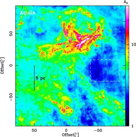
Figure 3: LOS-uncorrected column density of the Aquila cloud expressed in visual extinction. The white dashed rectangle indicates the region used for evaluating the LOS-contamination by (i) taking the mean of all pixels inside the rectangle (A_V=2.5) and (ii) constructing an N-PDF from these pixels and determining the peak of the distribution (A_V=2.4, see Figure 4).

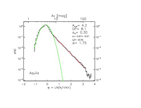
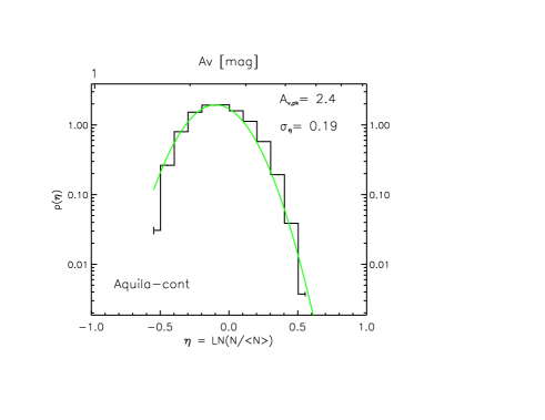
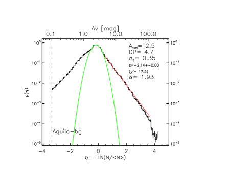
Figure 4: N-PDFs obtained from the LOS-uncorrected column density map (top), from the pixels within the white rectangle from Fig. 3 (middle), and from the LOS-corrected column density map (bottom).

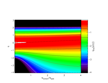
Figure 5: Two-dimensional representation of the N-PDFs of contaminated clouds after applying the constant screen correction as a function of the ratio between the contamination strength $N_{contam}$ and the typical cloud column density $N_{peak}$. The width of the cloud N-PDF was assumed to be $\sigma_{\eta,cloud}=0.5$ and the width of the contamination $\sigma_{\eta,cont}=0.15$, using some typical values for the clouds in this paper. The N-PDFs are represented through colors showing the logarithm.

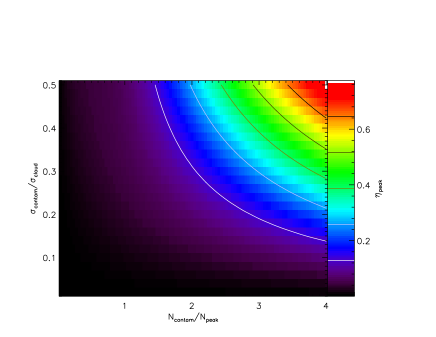
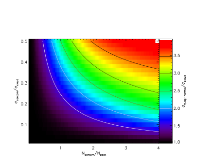
Figure 6: Parameters of the N-PDFs of contaminated clouds corrected for the contamination through the subtraction of a constant offset given by the peak of the N-PDF of the contaminating structure. The upper plot shows the position of the N-PDF peak on the logarithmic column density scale $\eta$ relative to the original peak column of the cloud. Consequently a value of 0 represents the correct peak position; a value of 0.5 indicates a 65 % overestimate of the column. The lower plot shows the width of the corrected cloud N-PDF relative to the original cloud N-PDF. On the horizontal axis, we varied the amplitude of the contamination, while on the vertical axis its width relative to the cloud N-PDF width.

Appendix B Significance of fitted models and slope comparison

B.1 BIC information

Tables 5 and 6 give the Bayesian information criterion (BIC) values and the weights, respectively, for the clouds in the study that were analyzed with method 4. The most likely model is the one with the lowest BIC values and the ratios of the weights gives a measure of how favored a model is compared to another. There are some models with a weight of 0 because it is just so low.

Table 5: Bayesian information criterion values for all clouds and for all models. The model with the minimum BIC is shown in bold. We note that for Draco, no PLT could be fit, the most likely model is the ELL one with a BIC of -382.2. Other models (EL, L, LL, LP etc.) have higher BICs.

Model	ELP	ELLP	EL2P	ELL2P	LP	LLP	L2P	LL2P
High-mass SF regions
Cygnus North	-503.88	-871.82	-719.87	-914.78	8671.25	41.67	8300.31	-174.01
Cygnus South	-309.28	-608.02	-318.54	-617.44	11267.88	715.80	9802.92	707.52
M16	23.91	-536.85	-123.23	-406.03	1210.30	-307.46	1045.74	-190.63
M17	4356.28	264.01	3212.22	98.91	23378.30	5528.30	19586.52	5642.49
NGC6334	8063.80	-236.74	7851.92	-542.82	61030.20	3553.64	51465.35	3469.84
NGC6357	3563.59	-226.32	3541.21	-250.39	14412.52	6246.08	11648.62	4234.76
NGC7538	483.82	71.95	25.69	-64.33	2687.11	607.64	1798.76	601.15
Rosette	-92.52	-518.24	-416.58	-546.29	1293.80	167.18	1033.42	175.69
Vela C	575.47	-105.57	116.86	-352.96	8364.11	1178.53	2497.10	87.91
Intermediate-mass SF regions
Aquila	-283.75	-618.65	-415.31	-749.90	15509.10	991.36	13294.37	890.44
MonR2	221.51	-65.93	-447.38	-503.61	8809.96	-299.52	7972.57	-410.60
MonOB1	4339.68	116.11	4239.46	-176.29	10159.28	774.17	10044.87	311.15
NGC2264	277.97	216.35	216.46	75.87	10524.29	745.90	10105.42	1106.19
Orion B	149.43	86.70	-470.14	-542.29	144.98	129.05	-474.24	-492.82
Serpens	1099.54	145.28	546.30	90.14	23029.18	2674.87	19708.70	2617.06
Low-mass SF regions
ChamI	9394.67	372.33	134.39	217.27	43476.62	1435.52	3104.40	1321.47
ChamII	404.72	-264.60	324.52	-361.85	9221.02	-148.55	7.01	-237.61
IC5146	2062.21	1964.76	216.23	-365.36	2258.17	2058.07	339.46	-265.88
Lupus I	117.50	75.00	-23.75	-36.72	16701.75	423.47	1761.06	542.80
Lupus III	208.33	-160.58	-103.01	-178.68	280.77	-43.10	-22.35	-116.40
Lupus IV	-113.56	-366.87	-320.08	-425.10	47.10	-145.50	-46.51	-350.43
Perseus	155.23	-359.51	-446.61	-441.65	1419.38	-330.10	-454.69	-442.44
Pipe	-152.55	-311.61	-320.53	-375.61	-156.14	-281.39	-304.53	-376.78
$\rho$Oph	12934.22	12189.37	450.90	-248.50	12928.56	12182.47	443.59	-254.23
Taurus	2085.79	2079.25	-290.70	-352.77	2314.11	2026.09	-99.35	-356.92
Quiescent regions
ChamIII	109.96	-470.85	5.27	-487.08	273.33	-317.40	-3.95	-333.85
Musca	3406.39	-347.94	-307.86	-350.00	8338.84	-180.95	-221.75	-352.48
Polaris	-245.60	-353.62	-258.46	-359.30	-194.85	-315.35	-217.47	-318.71

Table 6: Bayesian information criterion weight values for all clouds and for all models. The most likely model is denoted by its weight being bold. If the second most likely model has a weight within a factor of 10 of the most likely model (i.e. may be an alternative model) it is shown with an italic, bold weight. We note that for Draco, no PLT could be fit, the most likely model is the ELL one with a weight of 9.826514e-01. Other models (EL, L, LL, LP etc.) have higher weights.

Model	ELP	ELLP	EL2P	ELL2P	LP	LLP	L2P	LL2P
High-mass SF regions
Cygnus North	5.946e-90	4.692e-10	4.741e-43	1.000e+00	0.000e+00	2.039e-208	0.000e+00	1.393e-161
Cygnus South	1.202e-67	8.924e-03	1.233e-65	9.911e-01	0.000e+00	3.067e-290	0.000e+00	1.926e-288
M16	1.708e-122	1.000e+00	1.526e-90	3.916e-29	0.000e+00	1.544e-50	0.000e+00	6.596e-76
M17	0.000e+00	1.409e-36	0.000e+00	1.000e+00	0.000e+00	0.000e+00	0.000e+00	0.000e+00
NGC6334	0.000e+00	3.432e-67	0.000e+00	1.000e+00	0.000e+00	0.000e+00	0.000e+00	0.000e+00
NGC6357	0.000e+00	5.933e-06	0.000e+00	1.000e+00	0.000e+00	0.000e+00	0.000e+00	0.000e+00
NGC7538	9.348e-120	2.554e-30	2.834e-20	1.000e+00	0.000e+00	1.212e-146	0.000e+00	3.111e-145
Rosette	2.911e-99	8.076e-07	6.816e-29	9.999e-01	0.000e+00	1.177e-155	0.000e+00	1.665e-157
Vela C	2.477e-202	1.905e-54	9.547e-103	1.000e+00	0.000e+00	0.000e+00	0.000e+00	1.846e-96
Intermediate-mass SF regions
Aquila	5.982e-102	3.158e-29	2.212e-73	1.000e+00	0.000e+00	0.000e+00	0.000e+00	0.000e+00
MonR2	3.485e-158	9.099e-96	6.163e-13	1.000e+00	0.000e+00	4.813e-45	0.000e+00	6.355e-21
MonOB1	0.000e+00	3.207e-64	0.000e+00	1.000e+00	0.000e+00	4.076e-207	0.000e+00	1.425e-106
NGC2264	1.302e-44	3.127e-31	2.960e-31	1.000e+00	0.000e+00	3.198e-146	0.000e+00	1.857e-224
Orion B	6.236e-151	2.609e-137	2.152e-16	1.000e+00	5.771e-150	1.661e-146	1.672e-15	1.810e-11
Serpens	6.480e-220	1.063e-12	8.833e-100	1.000e+00	0.000e+00	0.000e+00	0.000e+00	0.000e+00
Low-mass SF regions
ChamI	0.000e+00	2.148e-52	1.000e+00	1.007e-18	0.000e+00	2.905e-283	0.000e+00	1.694e-258
ChamII	3.479e-167	7.628e-22	9.050e-150	1.000e+00	0.000e+00	4.814e-47	8.000e-81	1.051e-27
IC5146	0.000e+00	0.000e+00	5.121e-127	1.000e+00	0.000e+00	0.000e+00	8.918e-154	2.501e-22
Lupus I	3.243e-34	5.491e-25	1.524e-03	9.985e-01	0.000e+00	1.176e-100	0.000e+00	1.439e-126
Lupus III	9.158e-85	1.174e-04	3.702e-17	9.999e-01	1.705e-100	3.623e-30	1.131e-34	2.992e-14
Lupus IV	2.238e-68	2.267e-13	1.567e-23	1.000e+00	2.905e-103	1.930e-61	6.169e-83	6.104e-17
Perseus	3.530e-133	2.099e-21	1.725e-02	1.444e-03	0.000e+00	7.782e-26	9.792e-01	2.134e-03
Pipe	1.308e-49	4.531e-15	3.919e-13	3.578e-01	7.876e-49	1.242e-21	1.315e-16	6.422e-01
Taurus	0.000e+00	0.000e+00	3.708e-15	1.116e-01	0.000e+00	0.000e+00	1.042e-56	8.884e-01
Quiescent regions
ChamIII	2.261e-130	2.989e-04	1.223e-107	9.997e-01	7.567e-166	1.427e-37	1.229e-105	5.326e-34
Musca	0.000e+00	7.418e-02	1.469e-10	2.078e-01	0.000e+00	4.063e-38	2.941e-29	7.180e-01
Polaris	1.931e-25	5.520e-02	1.197e-22	9.448e-01	1.843e-36	2.702e-10	1.504e-31	1.450e-09

B.2 Comparison between different slope determinations

As pointed out in Sec. 2.4.1, the three methods used to fit the N-PDF differ in their premises. In contrast to Methods 1 and 2, the adapted BPLFIT technique (Method 3, see Veltchev et al. (2019) extracts possible PLTs, without any assumption on the rest of the distribution. Marinkova et al. (2020; in preparation) modified this technique further – through introduction of varying lower and upper density cutoffs – to allow for extraction of a second PLT.

It is therefore instructive to compare the slopes obtained through Method 3 with those from the other two. In general, the BPLFIT slopes correlate well with their counterparts. Method 2 extracts only single PLTs but some of them are identified with the first PLT (with a single exception) obtained through Method 3 (right panel). A few more significant discrepancies are due to differences between the estimated DPs. Methods 1 and 3 agree on the existence of two PLTs in eight studied regions of all types, with a good agreement between the obtained slope values (open squares in the left panel). For the rest of the regions, the first PLTs from Method 1 are typically identified with single PLTs extracted by Method 3 (filled triangles). The correlation between the slope values is even better than in the regions for which both techniques extract two PLTs.

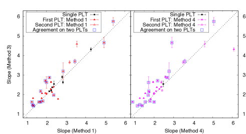
Figure 7: Comparison of slope estimations from the three PLTs fitting methods described in Sec. 2.4.1. Absolute slope values are given and the identity line is plotted as a dashed line. Different symbols are used for one or two PLTs. We note that the methods do not always agree on the number of PLTs.

Appendix C Column density maps, N-PDFs and $\Delta$-variance spectra

Figures C.1-C.29 display the column density maps expressed in visual extinction on the left and the $\Delta$-variance and N-PDF on the right. The plot range is 0.5 to 200 in A_V for high-mass SF molecular clouds. Since all these clouds are affected by LOS contamination, we show the corrected column density maps and N-PDFs. The plot range for intermediate-mass SF clouds is 0.5 to 100 in A_V, for low-mass SF clouds 0.1 to 20 in A_V, for quiescent clouds 0.1 to 10 in A_V, and for Draco 0.1 to 2 in A_V. The N-PDFs are presented as they are without the fits to the log-normal part and PLT(s). These are shown separately in Appendix D. As outlined in Sec. 2.4, the values of the slope(s) of the PLT(s), the DP and the width of the log-normal part are taken from the fit of method 4.

Figure 14: NGC7538: Fig. caption see Fig. C.1.

Appendix D Individual N-PDFs

Figures D.1 to D.29 display the N-PDFs of all clouds and the best fitting model. For all regions where we applied a LOS correction, we used this column density for performing the N-PDF. The models are indicated in the figure caption and follow the syntax explained in Sec. 2.4.1, (1) ELP: a single log-normal (L) convolved with a Gaussian noise distribution that creates an error slope (E) on the left-hand side and a power law tail (P); (2) ELLP: the same as (1) but with two log-normals, (3) LL2P: Two log-normals and two PLTs, (4) EL2P: the same as (1) but with two PLTs, (5) ELL2P: the same as (2) but with 2 PLTs.

Appendix E Correlations of N-PDF parameters with cloud type

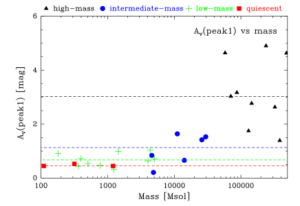
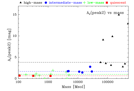
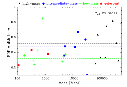
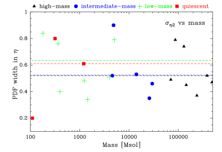
Figure 51: Correlation plots of N-PDF parameters as a function of mass as a proxy for the cloud type. The different cloud types are indicated with different colors and symbols. The median value for each cloud type is given in the respective color as a dashed line.

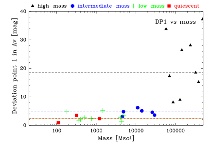
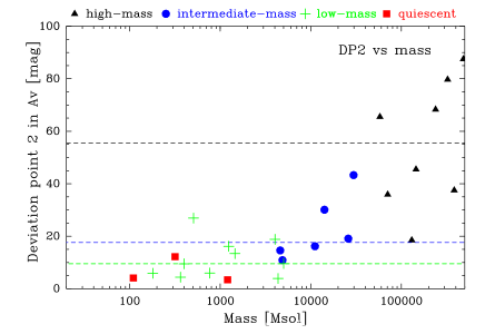
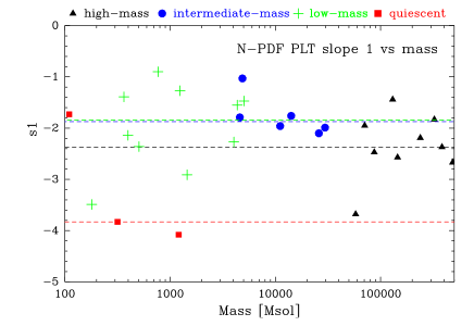
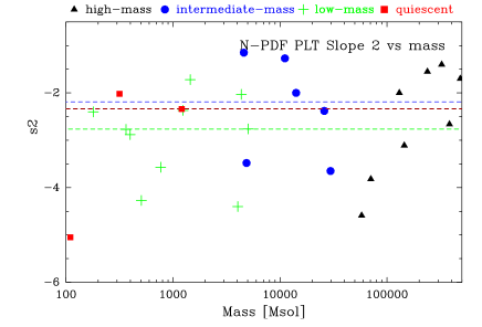
Figure 52: Correlation plots of N-PDF parameters as a function of mass as a proxy for the cloud type. The different cloud types are indicated with different colors and symbols. The median value for each cloud type is given in the respective color as a dashed line.

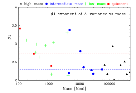
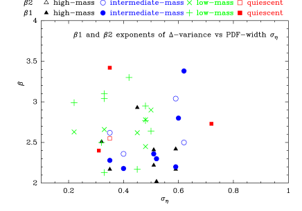
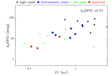
Figure 53: Correlation plots of $\beta_{1}$ and $\beta_{2}$ as a function of mass (top) as a proxy for the cloud type. The different cloud types are indicated with different colors and symbols. The median value for each cloud type is given in the respective color as a dashed line. The left bottom panel shows $\beta_{1}$ and $\beta_{2}$ against the width of the log-normal part of the N-PDF. The right bottom panel displays A_V(DP2) against P1 and indicates the A_V value where the slope change between first and second PLT in the N-PDF occurs, and the first characteristic size scale detected by the $\Delta$-variance.

Figures 51, 52 and  53 display various N-PDF parameters and the exponents $\beta_{1}$ and $\beta_{2}$ determined using the $\Delta$-variance given in Table 3 as a function of cloud mass as a proxy for cloud type. With these correlation plots, we explore possible systematic trends or thresholds.

Overall, we observe that the peak(s) of the N-PDF, A_V(peak1) and A_V(peak2), and the first and second deviation point, A_V(DP1) and A_V(DP2), increase with mass while all other parameters, the N-PDF width ($\sigma$), PLT slopes ($s_{1}$ and $s_{2}$) and $\beta_{1}$ and $\beta_{2}$ are rather independent of cloud type.

In Paper I, we fitted a single log-normal distribution at low column densities and derived that A_V(peak) increases with cloud mass. Here, we mostly fit two lognormals. The first peak for quiescent and low-mass regions is always below A_V$\sim 1$ while the second peak varies between A_V$\sim$0.5 and 2. Both parameters show no dependence on mass, which would be consistent with our interpretation that the first log-normal is mostly constituted by atomic gas. For intermediate- and high-mass regions, the A_V for the first and second peak are overall higher, but there is no trend of an increase with mass. This would support the proposal that for high-mass and intermediate-mass regions, the second peak of the N-PDF can be attributed to a compressed layer of dense gas due to stellar feedback. The (column)-density of this layer depends on various factors such as external pressure, initial density etc. and can thus vary from cloud to cloud.

The widths of the log-normal parts of the N-PDF show no clear trends. There is a tendancy that quiescent and low-mass regions have smaller $\sigma_{\eta 1}$ (median values of 0.38 and 0.32 with respect to intermediate and high mass regions with $\sigma_{\eta 1}$ = 0.47 and 0.52, respectively). The width of the second log-normal is generally larger, median values for all cloud types range betweem 0.52 and 0.64.

The A_V value where the log-normal fit to the low column density part of the N-PDF crosses the observed N-PDF and the first PLT starts is defined as the first deviation point, A_V(DP1). Ignoring the A_V(DP1) numbers for the most massive clouds (black triangles in Fig. 51), we find that the values cover a rather narrow range between A_V(DP1)$\sim$1 and A_V(DP1)$\sim$5 with a clustering around A_V(DP1)$\sim$2–5. These values are similar to those obtained by Kainulainen et al. (2011) using extinction maps, but slightly lower than the value of A_V=6.0$\pm$1.5 of Froebrich & Rowles (2010), also derived from extinction maps, and those of Paper I with A_V=4.7$\pm$0.4. To determine A_V(DP1) for massive clouds is delicate because if a second log-normal (or a ”bump” in the N-PDF) occurs due to compression, it may hide an underlying PLT. In other words, the transition from a turbulence-dominated regime (log-normal N-PDF) into a gravity-dominated one (PLT) may occur at values around A_V.

References

- Abreu-Vicente et al. (2017) Abreu-Vicente, J., Stutz, A., Henning, Th., et al., 2017, A&A, 604, 65
- Alves de Oliveira et al. (2014) Alves de Oliveira, C., Schneider, N., Merin, B., et al., 2014, A&A,
- Alves et al. (2014) Alves, J., Lombardi, M., Lada, C.J., 2014, A&A, 565, A18
- Alves et al. (2017) Alves, J., Lombardi, M., Lada, C.J., 2017, A&A, 606, L2
- André et al. (2010) André, Ph., Menshchikov, A., Bontemps S., et al., 2010, A&A, 518, L102
- André et al. (2014) André, Ph., Di Francesco, J., Ward-Thompson, D., et al., 2014, Protostars and Planets VI, University of Arizona Press (2014), eds. H. Beuther, R. Klessen, Dullemond, Th. Henning,
- Arshakian & Ossenkopf (2016) Arshakian, T.G., Ossenkopf, V., 2016, A&A, 585, 98
- Arzoumanian et al. (2011) Arzoumanian, D., André, Ph., Didelon, P., et al., 2011, A&A, 529, L1
- Auddy et al. (2018) Auddy, S., Basu, S., Kudoh, T., 2018, MNRAS, 474, 400
- Auddy et al. (2019) Auddy, S., Basu, S., Kudoh, T., 2019, MNRAS, 881, L15
- Ballesteros-Paredes et al. (1999) Ballesteros-Paredes, J., Hartmann, L., Vazquez-Semadeni, E., 1999, ApJ, 527, 285
- Ballesteros-Paredes et al. (2011) Ballesteros-Paredes, J., Vázquez-Semadeni, E., Gazol, A., 2011, MNRAS, 416, 1436
- Beattie et al. (2019) Beattie, J.R., Federrath, C., Klessen, R.S., Schneider, N., 2019, MNRAS, 488, 2493
- Benedettini et al. (2015) Benedettini, M., Schisano, E., Pezzuto, S., et al., 2015, MNRAS, 453, 2036
- Benedettini et al. (2018) Benedettini, M., Pezzuto, S., Schisano, E., et al., 2018, A&A, 619, 52
- Bensch et al. (2001) Bensch, F., Stutzki, J., Ossenkopf, V., 2001, A&A, 266, 636
- Bernard et al. (2010) Bernard, J.-Ph., Paradis, D., Marshall, D.J., et al., 2010, A&A, 518, L88
- Bergin & Tafalla (2007) Bergin, E. A., Tafalla, M., 2007, ARA, 26, 45, 339
- Berkhuijsen & Fletcher (2008) Berkhuijsen, E.M., Fletcher, A., 2008, MNRAS, 390, L19
- Bialey et al. (2017) Bialy, S., Burkhart, B., Sternberg, A., 2017, ApJ, 843, 92
- Bisbas et al. (2019) Bisbas, T., Schruba, A., van Dishoeck, E. F., 2019, MNRAS, 485, 3097
- Bohlin et al. (1978) Bohlin, R.C., Savage, B.D., Drake, J.F., 1978, ApJ 224, 132
- Bonne et al. (2020) Bonne, L., Schneider, N., Bontemps, S., et al., 2020, A&A, 641, 17
- Bontemps et al. (2010a) Bontemps, S., Motte F., Csengeri T., et al., 2010a, A&A, 524, 18
- Bontemps et al. (2010b) Bontemps, S., André P., Könyves V., Menshchikov A., et al., 2010b, A&A, 518, L85
- Brunt (2015) Brunt, C.M., 2015, MNRAS, 449, 4, 4465
- Butler et al. (2014) Butler, M.J., Tan, J.C., Kainulainen, J., 2014, ApJ, 224, 132
- Burkhart et al. (2012) Burkhart, B., Lazarian, A., 2012, ApJ, 755, L19
- Burkhart et al. (2015b) Burkhart, B., Lee, M.-Y., Murray, C., Stanimirovic, S., 2015, ApJ, 811, L28
- Burkhart et al. (2015a) Burkhart, B., Collins, D.C., Lazarian, A., 2015, ApJ, 808, 48
- Burkhart et al. (2017) Burkhart, B., Staples, K., Collins, D.C., 2017, ApJ, 834, L1
- Burkhart (2018) Burkhart, B., 2018, ApJ, 863, 118
- Burkhart & Mocz (2019) Burkhart, B., Mocz, P., 2019, ApJ, 879, 129
- Cambrésy et al. (2013) Cambrésy, L., Marton, G., Feher, O., et al., 2013, A&A, 557, 29
- Carlhoff et al. (2013) Carlhoff, P., Schilke P., Nguyen-Luong Q., et al., 2013, A&A, 560, 24
- Chen et al. (2018) Chen, H.H.-H., Burkhart, B., Goodman, A., Collins, D.C., 2018, ApJ, 859, 162
- Cho et al. (2011) Cho, W., Kim, J., 2011, MNRAS, 410, L8
- Clark et al. (2012) Clark, P.C., Glover, S.C.O., Klessen, R.S., Bonell, I.A., 2012, MNRAS, 424, 2599
- Collins et al. (2012) Collins, D.C., Kritsuk, A., Padoan, P. et al., 2012, ApJ, 750, 13
- Comeron et al. (2022) Comeron, F., Djupvik, A.A., Schneider N., 2022, A&A in press, arxiv:22030.7634
- Cox et al. (2016) Cox, N., Arzoumainian, D., André, Ph., et al., 2016, A&A, 590, 110
- Dib & Burkert (2005) Dib, S., Burkert, A., 2005, ApJ, 630, 238
- Dib et al. (2007) Dib, S., Kim, J., Vazquez-Semadeni, E., 2007, ApJ, 661, 262
- Dib et al. (2020) Dib, S., Bontemps, S., Schneider, 2020, A&A, 642, 177
- Didelon et al. (2015) Didelon, P., Motte F., Tremblin, P., et al., 2015, A&A, 584, 4
- DiFrancesco et al. (2010) Di Francesco, J., Sadavoy, S., Motte, F., et al., 2010, A&A, 518, L91
- Donkov et al. (2012) Donkov, S., Veltchev, T., Klessen, R.S., 2012, MNRAS, 423, 889
- Donkov et al. (2021) Donkov, S., Stefanov, I.Zh., Veltchev, T.V., Klessen, R.S., MNRAS, 505, 3655
- Elmegreen (2011) Elmegreen, B.G., 2011, ApJ, 731, 61
- Fallscheer et al. (2013) Fallscheer, C., Reid, M.A., Di Francesco, J., et al., 2013, ApJ, 773, 102
- Federman et al. (1979) Federman, S.R., Glassgold, A.E., Kwan, J., 1979, ApJ, 227, 466
- Federrath et al. (2008) Federrath, C., Klessen, R.S., Schmidt, W., 2008, ApJ, 688, L79
- Federrath et al. (2010) Federrath, C., Roman-Duval, J., Klessen, R.S., et al., 2010, A&A, 512, 81
- Federrath et al. (2011) Federrath, C., Sur, S., Schleicher, D., et al., 2011, ApJ, 731, 62
- Federrath & Klessen (2012) Federrath, C., Klessen, R.S., 2012, ApJ, 761, 156
- Federrath & Klessen (2013) Federrath, C., Klessen, R.S., 2013, ApJ, 763, 51
- Fiorellino et al. (2021) Fiorellino, E., Elia, D.;, André, Ph., et al., 2021, MNRAS, 500, 4, 4257
- Foster &Chevalier (1993) Foster, P.N., Chavalier, R.A., 1993, ApJ, 416, 303
- Froebrich et al. (2010) Froebrich, D., Rowles, J., 2011, MNRAS, 406, 1350
- Galvan-Madrid et al. (2010) Galvan-Madrid, R., Zhang, Q., Keto, E., et al., 2012, ApJ, 2010, 725, 17
- Giannini et al. (2012) Giannini, T., Elia, D., Lorenzetti, D., et al., 2012, A&A, 539, 156
- Gillmon et al. (2006) Gillmon, K., Shull, J.M., Tumlinson, J., Danforth, C., 2006, ApJ, 636, 891
- Girichidis et al. (2014) Girichidis, P., Konstandin, L., Whitworth, A.P., Klessen, R.S., et al., 2014, ApJ, 781, 91
- Glover & Mac Low (2007) Glover, S.C.O., Mac Low, M.-M., 2007, ApJ, 659, 1317
- Glover et al. (2010) Glover, S.C.O., Federrath, C., Mac Low, M.-M, Klessen, R.S., 2010, MNRAS, 404, 2
- Griffin et al. (2010) Griffin, M., Abergel, A., Abreu-Vicente, A., et al., 2010, A&A, 518, L3
- Hartmann et al. (2001) Hartmann, L., Ballesteros-Paredes, J., Bergin, E.A., 2001, ApJ, 562, 852
- Heiderman et al. (2010) Heiderman, A., Evans, N.J. II, Allen, L.E., et al., 2010, ApJ, 723, 1019
- Heitsch et al. (2001) Heitsch, F., Mac Low, M.-M, Klessen, R. S., 2001, ApJ, 547, 280
- Heitsch et al. (2005) Heitsch, F., Burkert, A., Hartmann, L., et al., 2005, ApJ, 633, 113
- Hennebelle & Chabrier (2008) Hennebelle, P., Chabrier, G., 2008, ApJ, 684, 395
- Hennebelle & Chabrier (2009) Hennebelle, P., Chabrier, G., 2009, ApJ, 702, 1428
- Hennemann et al. (2010) Hennemann, M., Motte, F., Bontemps, S., et al., 2010, A&A, 518, L84
- Hennemann et al. (2012) Hennemann, M., Motte, F., Schneider, N., et al., 2012, A&A, 543, L3
- Herbstmeier et al. (1993) Herbstmeier, U., Heithausen, A., Mebold, U., 1993, A&A, 272, 514
- Hill et al. (2011) Hill, T., Motte, F., Didelon, P., et al., 2011, A&A, 533, 94
- Hill et al. (2012) Hill, T., Motte, F., Didelon, P., et al., 2012, A&A, 542, 114
- Hopkins (2012) Hopkins, P.F., 2012, MNRAS, 423, 2037
- Imara & Burkhart (2016) Imara, N., Burkhart, B., 2016, ApJ, 829, 102
- Jaupart & Chabrier (2020) Jaupart, E. & Chabrier, G., 2020, ApJL, 903, L2
- Jaupart & Chabrier (2022) Jaupart, E. & Chabrier, G., 2022, A&A, in press, arXiv:2205.12571
- Juvela et al. (2015) Juvela, M., Ristorcelli, I., Marshall, D. J., et al., 2015, A&A, 584, 93
- Kabanovic et al. (2022) Kabanovic, S., Schneider, N., Ossenkopf-Okada, V., et al., 2022, A&A, 659, 36
- Kainulainen et al. (2009) Kainulainen, J., Beuther, H., Henning, T., Plume, R., 2009, A&A, 508, L35
- Kainulainen et al. (2011) Kainulainen, J., Beuther, H., Banerjee, R., et al., 2011, A&A, 530, 64
- Kainulainen et al. (2013) Kainulainen, J., Tan, J., 2013, A&A, 53, 549
- Khullar et al. (2021) Khullar,S., Federrath, C., Krumholz, M.R., Matzner, C.D., 2021, MNRAS, 507, 4335
- Klessen (1997) Klessen, R.S., 1997, MNRAS, 292, 11
- Klessen (2000) Klessen, R.S., 2000, ApJ, 535, 869
- Klessen et al. (2000) Klessen, R.S., Heitsch, F., Mac Low, M.-M., 2000, ApJ, 535, 887
- Klessen & Glover (2016) Klessen, R.S., Glover, S.O.C., 2016, Star Formation in Galaxy Evolution: Connecting Numerical Models to Reality, Saas-Fee Advanced Course, Vol. 43, p. 85
- Kirk et al. (2013) Kirk, J.M., Ward-Thompson, D., Palmeirim, P., et al., 2013, MNRAS, 432, 1424
- Könyves et al. (2010) Könyves, V., André, Ph., Menshchikov, A., et al., 2010, A&A, 518, L106
- Könyves et al. (2015) Könyves, V., André, Ph., Menshchikov, A., et al., 2015, A&A, 584, 91
- Könyves et al. (2020) Könyves, V., André, Ph., Arzoumanian, D., , et al., 2020, A&A, 635, 34
- Körtgen et al. (2019) Körtgen, B., Federrath, C., Banerjee, R., 2019, MNRAS, 482, 5233
- Koyama & Inutsuka (2000) Koyama, H., Inutsuka, S.-I., 2000, ApJ, 532, 980
- Kritsuk et al. (2011) Kritsuk, A.G., Norman, M.L., Wagner, R., 2011, ApJ, 727, L20
- Krumholz & McKee (2008) Krumholz, M., McKee, C.F., 2008, Nature, 451, 1082
- Krumholz & McKee (2020) Krumholz, M., McKee, C.F., 2020, MNRAS, 494, 624
- Lada et al. (2010) Lada, C.J., Lombardi, M., Alves, J., 2010, ApJ, 724, 687
- Ladjelate et al. (2020) Ladjelate, B., André, Ph., Könyves, V., A&A, 2020, 638, 74
- Lagache et al. (1998) Lagache, G., Abergel, A., Boulanger, F., Puget, J.-L., 1998, A&A, 333, 709
- Larson (1969) Larson, R.B., 1969, MNRAS, 145, 271
- Lee et al. (1996) Lee, H.-H., Herbst, E., Pineau de Fôrets, et al., 1996, A&A, 311, 690
- Lenz et al. (2015) Lenz, D., Kerp, J., Flöer, L., et al., 2015, A&A, 573, 83
- Lockman & Condon (2005) Lockman, F.J., Condon, J.J., 2005, AJ, 129, 1968
- Lombardi et al. (2008) Lombardi, M., Lada, C., Alves, J., 2008, A&A, 489, 143
- Lombardi et al. (2014) Lombardi, M., Bouy, H., Alves, J., Lada, C., 2014, A&A, 566, 45
- MacLow et al. (2004) Mac Low, M.M., Klessen, R., 2004, Reviews of Modern Physics, vol.76, Issue 1, 125-194
- Mandal et al. (2022) Mandal, A., Federrath, C., Körtgen, B., 2022, MNRAS, 493, 3, 3098
- Marinkova et al. (2021) Marinkova, L., Veltchev, T., Girichidis, P., Donkov, S., 2021, Astronomische Nachrichten, Vol. 342, number 6, p. 898
- Marsh et al. (2014) Marsh, K.A., Griffin, M., Palmeirim, P., et al., 2014, MNRAS, 439, 3683
- Marsh et al. (2016a) Marsh, K.A., Kirk, J.M., André, Ph., et al., 2016a, MNRAS, 459, 342
- Marsh et al. (2016b) Marsh, K.A., Whitworth, A.P., Lomax, O., et al., 2016b, MNRAS
- Menshchikov et al. (2010) Menshchikov, A., André, Ph., Didelon, P., et al., 2010, A&A, 518, L103
- Mebold et al. (1985) Mebold, U., Cernicharo, J., Velden, L., et al., 1985, A&A, 151, 427
- Meyerdierks et al. (1991) Meyerdierks, H., Heithausen, A., Reif, K., 1991, A&A, 245, 247