Archaeology of random recursive dags and Cooper-Frieze random networks

Abstract

We study the problem of finding the root vertex in large growing networks. We prove that it is possible to construct confidence sets of size independent of the number of vertices in the network that contain the root vertex with high probability in various models of random networks. The models include uniform random recursive dags and uniform Cooper-Frieze random graphs.

1 Introduction

With the ubiquitous presence of networks in many areas of science and technology, a multitude of new challenges have gained importance in the statistical analysis of networks. One such area, termed network archaeology (Navlakha and Kingsford [26]) studies problems about unveiling the past of dynamically growing networks, based on present-day observations.

In order to develop a sound statistical theory for such problems, one usually models the growing network by simple stochastic growth dynamics. Perhaps the most prominent such growth model is the preferential attachment model, advocated by Albert and Barabási [2]. In these models, vertices of the network arrive one by one and a new vertex attaches to one or more existing vertices by an edge according to some simple probabilistic rule.

Arguably the simplest problem of network archaeology is that of root finding, when one aims at estimating the first vertex of a random network, based on observing the (unlabeled) network at a much later point of time.

The existing literature on the theory of network archaeology mostly focuses on the simplest possible kind of networks, namely trees, see Haigh [20], Shah and Zaman [29, 28], Bubeck, Mossel, and Rácz [7], Curien, Duquesne, Kortchemski, and Manolescu [13], Khim and Loh [23], Jog and Loh [21, 22], Bubeck, Eldan, Mossel, and Rácz [9], Bubeck, Devroye, and Lugosi [8], Lugosi and Pereira [24], Devroye and Reddad [16], Banerjee and Bhamidi [3], Crane and Xu [11], Addario-Berry, Devroye, Lugosi, and Velona [1], Brandenberger, Devroye, and Goh [5].

In various models of growing random trees, it is quite well understood up to what extent one may identify the origin of the tree (i.e., the root) by observing a large unlabeled tree. These models include uniform and linear preferential attachment trees and diffusion over regular trees. Remarkably, in all these models, the size of the tree does not play a role. In other words, there exist root-finding algorithms that are able to select a small number of nodes – independently of the size of the tree – such that the root vertex is among them with high probability.

Here we address the more difficult – and more realistic – problem of finding the origin of growing networks when the network is not necessarily a tree. The added difficulty stems from the fact that the centrality measures that proved to be successful in root estimation in trees crucially rely on properties of trees.

A notable exception in the literature is the recent paper of Crane and Xu [12] in which the authors allow for a “noisy” observation of the tree. In their model, the union of the tree of interest and an (homogeneous) Erdős-Rényi random graph is observed, and the goal is to estimate the root of the tree.

In this paper we study root estimation in two more complex network models. Both of these models may be viewed as natural extensions of the random recursive trees that were in the focus of most of the previous study of network archaeology. Recall that a uniform random recursive tree on the vertex set $[n]$ is defined recursively, such that each vertex $i\in\{2,3,\ldots,n\}$ is attached by an edge to a vertex chosen uniformly at random among the vertices $\{1,\ldots,i-1\}$, see, e.g., Drmota [18].

In particular, we study the problem of root finding in (1) uniform random recursive dags; and (2) uniform Cooper-Frieze random graphs.

Uniform random recursive dags

For a positive integer $\ell$, a uniform random $\ell$-dag is simply the union of $\ell$ independent uniform random recursive trees on the same vertex set $[n]$. Equivalently, a uniform random $\ell$-dag may be generated recursively; each vertex $i\in\{2,3,\ldots,n\}$ is attached by an edge to $\ell$ vertices chosen uniformly at random (with replacement) among the vertices $\{1,\ldots,i-1\}$. Multiple edges are collapsed so that the resulting graph is simple. Random recursive dags have been studied by Díaz Cort, Serna Iglesias, Spirakis, Torán Romero, and Tsukiji [17], Tsukiji and Xhafa [31], Tsukiji and Mahmoud [30], Devroye and Janson [15], Broutin and Fawzi [6], Mahmoud [25], among others.

Definition 1.

Let $n,\ell\in\mathbb{N}$. For $i=[\ell]$, let $G_{i}=(V,E_{i})$ be independent uniform random recursive trees on the vertex set $V=[n]$. A uniform random recursive $\ell$-dag on $n$ vertices is $G=(V,E_{1}\cup\cdots\cup E_{\ell})$.

Uniform Cooper-Frieze random graphs

The other network model studied here was introduced by Cooper and Frieze [10] in an attempt to mathematically describe large web graphs, see also Frieze and Karoński [19]. In the Cooper-Frieze network model both vertices and edges are added sequentially to the network based on uniform or preferential attachment mechanisms. The model is quite general but here we focus on the simplest version when both vertices and edges are added by uniform attachment.

More precisely, the uniform Cooper-Frieze growth model is defined as follows. The procedure has a parameter $\alpha\in(0,1)$. The process is initialized by a graph containing a single vertex and no edges. At each time instance $t=1,2,\ldots$, an independent Bernoulli$(\alpha)$ random variable $Z_{t}$ is drawn. If $Z_{t}=0$, a new vertex is added to the vertex set along with an edge that connects this vertex to one of the existing vertices, chosen uniformly at random. If $Z_{t}=1$, then a new edge is added by choosing two existing vertices uniformly at random and connecting them. Note that the resulting graph may have multiple edges. In such cases, we may convert the graph into a simple graph by keeping only one of each multiplied edge.

If one runs the process for $T$ steps for a large value of $T$, the graph has $n\sim\text{Binomial}(T-1,1-\alpha)\approx(1-\alpha)T$ vertices and $T-1\approx n/(1-\alpha)$ edges. If one removes the edges added at the times when $Z_{t}=1$, the remaining graph is a tree, distributed as a uniform random recursive tree on $n$ vertices. The remaining $T-n-1$ edges are present approximately independently of each other and there is an edge between vertices $i$ and $j$ (where $1\leq i<j\leq n$) if

$$\sum_{t=1}^{T}\sum_{\ell=j}^{n}\mathbbm{1}_{t\in\{t_{\ell}+1,t_{\ell+1}-1\}}\mathbbm{1}_{\text{the pair $(i,j)$ is selected at time $t$}}\geq 1~{},$$

where $1=t_{1}<t_{2}<\cdots<t_{n}\leq T$ are the times when new vertices are added, that is, when $Z_{t}=1$. Since the probability that edge $(i,j)$ is selected at time $t\in\{t_{\ell}+1,t_{\ell+1}-1\}$ is $1/\binom{\ell}{2}$, for large values of $T$, the probability that edge $(i,j)$ is present in the graph after $T$ steps is concentrated around

$$\frac{c_{\alpha}}{\max(i,j)-1}\quad\text{where}\quad c_{\alpha}\stackrel{{\scriptstyle\mathrm{def.}}}{{=}}\frac{2}{1-\alpha}~{},$$

whenever $\max(i,j)-1\geq c_{\alpha}$. Hence, the uniform Cooper-Frieze model is essentially equivalent to the following random graph model. In order to avoid some tedious and uninteresting technicalities, we work with this modified model instead of the original recursive definition.

Definition 2.

Let $n\in\mathbb{N}$ and let $c$ be a positive constant. Let $G_{1}=(V,E_{1})$ be a uniform random recursive tree on the vertex set $V=[n]$. Let $G_{2}=(V,E_{2})$ be a random graph on the same vertex set, independent of $G_{1}$, such that edges of $G_{2}$ are present independently of each other, such that for all $i\neq j$,

$$\mathbb{P}\{(i,j)\in E_{2}\}=\min\left(\frac{c}{\max(i,j)-1},1\right)~{}.$$

Finally, the uniform Cooper-Frieze random graph with parameters $c$ and $n$ is $G=(V,E_{1}\cup E_{2})$.

Root estimation

The main result of this paper is that finding the root is possible both in uniform random recursive dags and in uniform Cooper-Frieze random graphs. More precisely, one may find confidence sets for the root vertex whose size does not depend on the number of vertices in the graph. To make such statements rigorous, consider the following definition.

Definition 3.

Let $\{G^{(n)}\}$ be a sequence of random graphs such that $G^{(n)}$ has vertex set $[n]$. We say that root estimation is possible if the following holds. For every $\epsilon>0$, there exists a positive integer $K(\epsilon)$ such that, for every $n\in\mathbb{N}$, upon observing the graph $G^{(n)}$ without the vertex labels, one may find a set $S\subset[n]$ of vertices of size $|S|=K(\epsilon)$ such that

$$\mathbb{P}\{1\in S\}\geq 1-\epsilon~{}.$$

The set $S$ in the above definiton is often called a confidence set for the root vertex.

As mentioned above, root estimation has mostly been studied for random recursive trees. Bubeck, Devroye, and Lugosi [8] show that root estimation is possible in the uniform random recursive tree and linear preferential attachment trees. They show that in the case of the uniform random recursive tree, one may take $K(\epsilon)\leq\exp\left(c\log(1/\epsilon)/\log\log(1/\epsilon)\right)$ for some constant $c$. For linear preferential attachment trees one may take $K(\epsilon)=c\epsilon^{-2-o(1)}$, as shown by Banerjee and Bhamidi [3] who also show that root estimation is possible for a wide class of preferential attachment trees. Building on the papers of Shah and Zaman [29, 28], Khim and Loh [23] show that root estimation is possible in random trees obtained by diffusion on an infinite regular tree, and that one my take $K(\epsilon)=\exp\left(O\left(\log(1/\epsilon)/\log\log(1/\epsilon)\right)\right)$. Brandenberger, Devroye, and Goh [5] study root estimation in size-conditioned Galton–Watson trees.

The sets $S$ of constant size that establish the possibility of root estimation for various trees usually contain the set of most “central” vertices according to some notion of centrality such as Jordan centrality (as in [8], [3]) or rumor centrality introduced in [29, 28], see also [8], [23]. However, these notions are suited for trees only and when the observed network is more complex, new ideas need to be introduced. Crane and Xu [12] study a model in which the observed network consists of either a uniform attachment tree (i.e., uniform random recursive tree) or a preferential attachment tree, with random edges added (independently over all possible vertex pairs, with the same probability). They introduce a Bayesian method and prove that it is able to estimate the root as long as there are not too many edges, where the threshold value depends on the particular model. It is unclear if the method of [12] may be generalized to the random graph models studied here. Instead, we introduce an alternative root estimation method that is based on the appearance of certain subgraphs.

The main results of this paper are summarized in the following two theorems.

Explicit values of the constants $c_{0},c_{1},c_{2}$ are given in the proof below. In the uniform Cooper-Frieze model we have a similar bound:

The main results establish that, upon observing the graph after removing its vertex labels, one may find a set $S$ of vertices of size independent of $n$ such that $S$ contains the root vertex (i.e., vertex $1$) with probability at least $1-\epsilon$. The size of the set is bounded by a function of $\epsilon$ only.

Observe that if $\ell$ is of the order of $\log(1/\epsilon)$, then the bound for $K(\epsilon)$ is $1/\epsilon$ times a poly-logarithmic term in $1/\epsilon$. On the other hand, when $\ell$ is a fixed constant, as $\epsilon\to 0$, the obtained bounds are super-polynomial in $1/\epsilon$, significantly larger than the analogous bounds obtained for uniform and preferential attachment trees. In all ranges of $\ell$, these bounds are inferior to the best upper bounds available for the case $\ell=1$ (i.e., uniform random recursive trees). We do not claim optimality of this bound. It is an interesting open question whether much smaller vertex sets may be found with the required guarantees. We conjecture that for any $\ell>1$, root finding is easier in a uniform random $\ell$-dag than in a uniform random recursive tree. If that is the case, one should be able to take $K(\epsilon)$ as $\exp\left(O\left(\log(1/\epsilon)/\log\log(1/\epsilon)\right)\right)$. Similar remarks hold for the bound of Theorem 2.

In order to prove Theorems 1 and 2, we propose a root estimation procedure and prove that the same procedure works in both models. The procedure looks for certain carefully selected subgraphs that we call double cycles. The set $S$ of candidate vertices are certain special vertices of such double cycles.

The rest of the paper is organized as follows. In Section 2 we introduce the proposed root estimation procedure. The proof of Theorem 1 is given in Section 3 while Theorem 2 is proved in Section 4.

2 Double cycles

In this section we define the root estimation method that we use to prove the main results. In order to determine the set $S$ of vertices that are candidates for being the root vertex, we define “double cycles”.

Let $s,t$ be positive integers. We say that a vertex $v\in[n]$ is an anchor of a double cycle of size $(s,t)$ if there exists an integer $0<p\leq\min(s,t)/2$ and $s+t-1-p$ different vertexes $i_{1},i_{2},\dots i_{s+t-2-p}\in[n]$, such that

$\bullet$ vertices $v,i_{1},\ldots,i_{s-1}$ form a cycle of length $s$ in $G$ (in this order);

$\bullet$ vertices $v,i_{s+1-p},\ldots,i_{s+t-1-p}$ form a cycle of length $t$ in $G$ (in this order).

Note that the two cycles are disjoint, except for the common path $v\sim\cdots\sim i_{p-1}$ (so $p$ is the number of common vertices in both cycles). Also note that $i_{p-1}$ is another anchor of the same double cycle. If $p=1$, we declare $i_{0}=v$. In that case the two cycles intersect in the single vertex $v$ and the double cycle has a unique anchor $v$, see Figure 1.

In other words, if two vertices $v,u\in[n]$ are connected by three disjoint paths such that the sum of the lengths of the first and second paths is $s$ and the sum of the lengths of the second and third paths is $t$, then $v$ and $u$ are anchors of a double cycle of size $s$ and $t$. Also, $v$ is the anchor of a double cycle of size $(s,t)$ if vertex $v$ is the unique common vertex of two cycles of lengths $s$ and $t$.

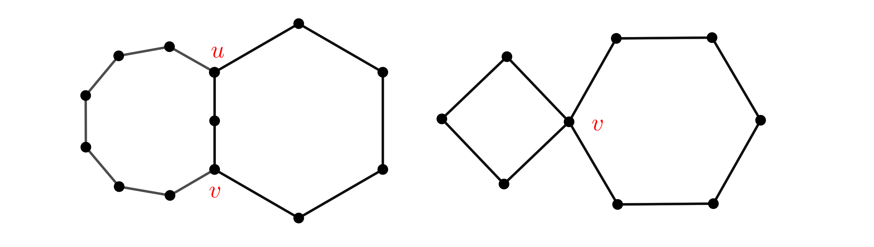
Figure 1: Examples of double cycles

For a positive integer $m$, let $S_{m}\subset[n]$ be the set of vertices $i$ such that $i$ is an anchor of a double cycle of size $(s,t)$ for some $s\leq m$ and $t\leq m$.

In order to prove Theorem 1, it suffices to show that for any given $\epsilon\in(0,1/100)$, one may take $m=m_{\epsilon}=\left\lceil\frac{30}{\ell}\log(1/\epsilon)\right\rceil$ such that

$$\mathbb{P}\left\{1\in S_{m}\ \text{and}\ |S_{m}|\leq\frac{4}{\epsilon}\ell^{2m}(2m)!\right\}\geq 1-\epsilon~{}.$$

This follows if we prove that we have both

$$\mathbb{P}\left\{1\in S_{m}\right\}\geq 1-\frac{\epsilon}{2}$$ (2.1)

and

$$\mathbb{P}\left\{|S_{m}|\leq\frac{4}{\epsilon}\ell^{2m}(2m)!\right\}\geq 1-\frac{\epsilon}{2}~{}.$$ (2.2)

We prove (2.1) in Section 3.1 and (2.2) in Section 3.2.

Remark 1.

The reader may wonder why the proposed method looks for double cycles as opposed to simpler small subgraphs such as triangles or a clique of size $4$ with an edge removed, etc. The reason is that such simpler subgraphs are either too abundant in the sense that vertices with high index may be contained in (many of) them or the root vertex is not contained in any of them with some probability that is bounded away from zero. This may happen in spite of the fact that the expected number of such small subgraphs containing the root vertex goes to infinity as $n\to\infty$. Double cycles guarantee the appropriate concentration expressed in (2.1).

3 Proof of Theorem 1

As it is explained in the previous section, in order to prove Theorem 1, it is enough to prove the inequalities (2.1) and (2.2), where $S_{m}$ is the set of those vertices that are anchors of a double cycle of size $(s,t)$ for some $s,t\leq m$.

3.1 The root vertex is the anchor of a small double cycle

First we consider the case when $\ell=2$. Then the observed graph $G$ is the union of two independent random recursive trees $T_{1}$ and $T_{2}$. To prove (2.1) we need to ensure that vertex $1$ is the anchor of a double cycle of small size, with probability at least $1-\epsilon/2$. To do so, it suffices to show that there are two edges $(1,i)$ and $(1,j)$ that are present in $T_{2}$ but not in $T_{1}$ where $i$ and $j$ are “small”– whose meaning is specified below. Indeed, in this case there are two cycles containing vertex $1$ formed as follows:

• the unique path from vertex $1$ to $i$ in $T_{1}$ loops back to $1$ thanks to edge $(1,i)$, present in $T_{2}$;

• the unique path from vertex $1$ to $j$ in $T_{1}$ loops back to $1$ thanks to edge $(1,j)$, present in $T_{2}$.

The only intersection of those two cycles is the intersection of the paths in $T_{1}$ from vertex $1$ to $i$ and from vertex $1$ to $j$. In a tree, the intersection of two paths is either empty or a path itself. Here the intersection is not empty since both paths contain vertex $1$. Thus, vertex $1$ is in two cycles which only intersect in a path having vertex $1$ as an extremity, meaning that vertex $1$ is the anchor of a double cycle. Next we show that two such edges indeed exist, with high probability.

For a vertex $i\in[n]$, the probability that the edge $(1,i)$ is present in $T_{2}$ is $1/(i-1)$. The probability that it is absent in $T_{1}$ is $1-1/(i-1)$. By independence of $T_{1}$ and $T_{2}$, the probability that the edge $(1,i)$ is present in $T_{2}$ and absent in $T_{1}$ is $\left(1-1/(i-1)\right)/(i-1)$. Let $X_{k}$ denote the number of edges of form $(1,i)$ for some $i\in[k]$ that are not edges in $T_{1}$. Then $X_{k}$ may be written as a sum of independent random variables,

$$X_{k}\ =\ \sum_{i=2}^{k}B_{i}$$

where $B_{i}$ is a Bernoulli random variable with parameter $\frac{1}{i-1}\left(1-\frac{1}{i-1}\right)$.

If $X_{k}\geq 2$, there exist two edges of form $(1,i)$ with $i\leq k$ that are not present in $T_{1}$. By a standard bound for the lower tail for for sums of nonnegative independent random variables, see [4, Exercise 2.9], we have

$$\mathbb{P}\left\{X_{k}\geq 2\right\}\ \geq\ 1-\exp\left(-\frac{\left(\mathbb{E}[X_{k}]-1\right)^{2}}{2\mathbb{E}[X_{k}]}\right)~{}.$$

Since $\mathbb{E}[X_{k}]$ is easily seen to fall between $\log(k)-2$ and $\log(k)-1$, we have

$$\mathbb{P}\left\{X_{k}\geq 2\right\}\ \geq\ 1-\exp\left(-\frac{1}{2}\log(k)+\frac{5}{2}-\frac{2}{\log(k)-1}\right)~{}.$$

Hence, for $k_{\epsilon}=\left\lceil 16e^{5}/\epsilon^{2}\right\rceil$, we have $\mathbb{P}\{X_{k_{\epsilon}}\geq 2\}\geq 1-\epsilon/4$. This implies that, with probability at least $1-\epsilon/4$, vertex $1$ is the anchor of a double cycle such that all vertices in the double cycle are in $[k_{\epsilon}]$. To conclude the proof of (2.1) we need to check that indeed the size of the double cycle containing vertex $1$ is at most $m$. Such double cycles are formed by a path in $T_{1}$, closed by an additional edge coming from $T_{2}$. Therefore, both cycles contained in the double cycle of interest have a size bounded by the height of the subtree of $T_{1}$ induced by the vertex set $[k_{\epsilon}]$, plus $1$. By well-known bounds for the height of a uniform random recursive tree (see, e.g., Drmota [18], Devroye [14], Pittel [27]) we have that the depth of a uniform random recursive tree on $k$ vertices is bounded by $e\log(k)+e\log(4e/\epsilon)$ with probability at least $1-\epsilon/4$, see Drmota [18, p. 284].

Plugging in the value of $k_{\epsilon}$, we get that for any $\epsilon\leq 10^{-2}$, the diameter of a uniform recursive random tree of size $k_{\epsilon}$ is at most $15\log(1/\epsilon)$, with probability at least $1-\epsilon/4$.

Putting these bounds together, we have that, in the case $\ell=2$, with probability at least $1-\epsilon/2$, vertex $1$ is an anchor of a double cycle of size $(s,t)$ with $s,t\leq 15\log(1/\epsilon)$, implying (2.1) for $\ell=2$.

It remains to extend the above to the general case of $\ell\geq 2$. Since $G$ is the union of $\ell$ independent uniform random recursive trees, it contains the union of $\lfloor\ell/2\rfloor$ independent, identically distributed random uniform $2$-dags. Using the result proved for random uniform $2$-dags above, the probability than in $G$, vertex $1$ is not the anchor of a double cycle of size at most $15\log(\epsilon^{2/(\ell-1)})$ is at most $\epsilon$. This concludes the proof of (2.1) in the general case.

3.2 High-index vertices are not anchors of double cycles

In order to prove (2.2) we need to show that no vertex with high index is the anchor of a double cycle of size smaller than $m$. We bound the probability that there exists $v>K$ such that $v\in S_{m}$, where recall that $K=K(\epsilon)$. To this end, we count $C_{s,t}(v)$, the number of double cycles of size $(s,t)$ having vertex $v$ as an anchor. Then, by the union bound,

$$\mathbb{P}\left\{\exists v>K:v\in S_{m}\right\}\leq\sum_{v\geq K}\sum_{s,t\leq m_{\epsilon}}\mathbb{P}\{C_{s,t}(v)\geq 1\}\leq\sum_{v\geq K}\sum_{s,t\leq m_{\epsilon}}\mathbb{E}C_{s,t}(v)~{}.$$ (3.1)

In order to bound $\mathbb{E}C_{s,t}(v)$, we may assume, without loss of generality, that $s\leq t$.

For a permutation $\sigma\in\Pi_{s+t-2-p}$, we denote by $C(s,t,p,v,\sigma,i_{1},\ldots,i_{s+t-p-2})$ the following event:

• if $p=1$,

  $$C(s,t,1,v,\sigma,i_{1},\ldots,i_{s+t-2})$$

  $$= \left\{v\sim i_{\sigma(1)}\sim\cdots\sim i_{\sigma(s-1)}\sim v\sim i_{\sigma(s)}\sim\cdots\sim i_{\sigma(s+t-2)}\sim v\right\}~{},$$

• and if $p>1$

  $$C(s,t,p,v,\sigma,i_{1},\ldots,i_{s+t-p-2})$$

  $$= \left\{v\sim i_{\sigma(1)}\sim\cdots\sim i_{\sigma(s-1)}\sim v\sim i_{\sigma(s)}\sim\cdots\sim i_{\sigma(s+t-2-p)}\sim i_{\sigma(s-p)}\right\}~{}.$$

where $i\sim j$ denotes that vertices $i$ and $j$ are joined by an edge. Thus, $C(s,t,p,v,\sigma,i_{1},\ldots,i_{s+t-p-2})$ is the event that the double cycle of size $s,t$ ($s\leq t$) having $p$ vertices in the intersection, with $v$ as an anchor and on the set of vertices $\{i_{1},\ldots,i_{s+t-p-2}\}$ ordered by $\sigma$ as illustrated in Figure 2 is present.

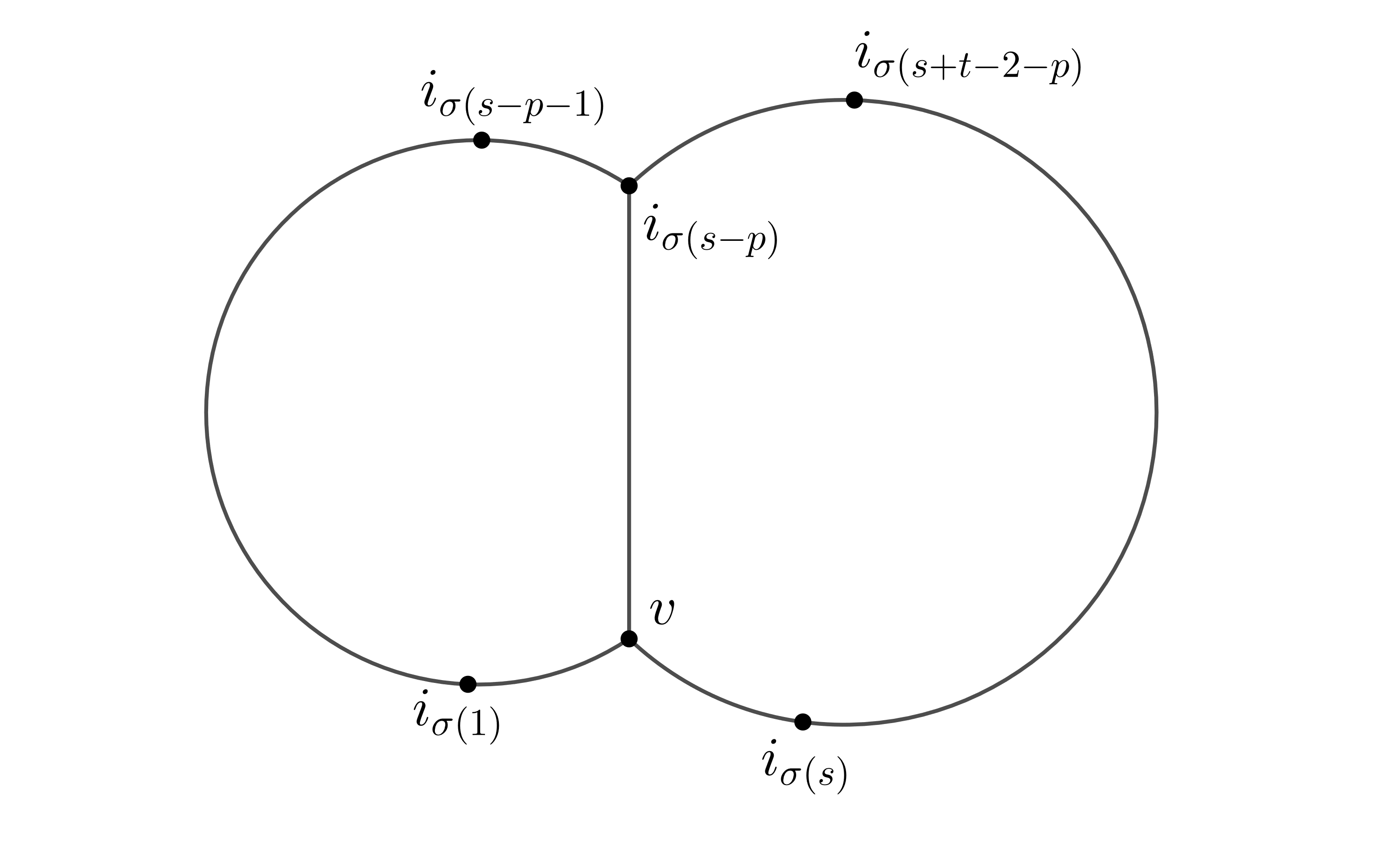
Figure 2: Index ordering in a double cycle

With this notation, we may write $C_{s,t}(v)$ as follows:

$$C_{s,t}(v)= \sum_{p=1}^{\lfloor s/2\rfloor}\ \ \ \sum_{i_{1}<\dots<i_{s+t-2-p}}\ \ \ \sum_{\sigma\in\Pi_{s+t-2-p}}\mathbbm{1}_{C(s,t,p,v,\sigma,i_{1},\ldots,i_{s+t-p-2})}~{},$$ (3.2)

in order to bound the expected number $\mathbb{E}C_{s,t}(v)$ of double cycles of size $(s,t)$ anchored at $v$, we need to estimate $\mathbb{P}\left\{C(s,t,p,v,\sigma,i_{1},\ldots,i_{s+t-p-2})\right\}$.

This exact probability is difficult to compute. Instead, we make use of the following proposition that establishes that a uniform random $\ell$-dag is dominated by an appropriately defined inhomogeneous Erdős-Rényi random graph. This random graph is defined as a graph on the vertex set $[n]$ such that each edge is present independently of the others and the probability that vertex $i$ and vertex $j$ are connected by an edge equals

$$\pi(i,j)\stackrel{{\scriptstyle\mathrm{def.}}}{{=}}\min\left(1,\frac{\ell}{\max(i,j)-1}\right)~{}.$$

The next proposition shows that every fixed subgraph is at most as likely to appear in a uniform random $\ell$-dag as in the inhomogeneous Erdős-Rényi random graph.

Proposition 1.

Let $G=(V,E)$ be a uniform random $\ell$-dag on the vertex set $V=[n]$. For some $k\leq\binom{n}{2}$, let $(a_{1},b_{1}),\ldots,(a_{k},b_{k})$ be distinct pairs of vertices such that $a_{i}\neq b_{i}$ for all $i\leq k$. Then

$$\mathbb{P}\left\{(a_{1},b_{1}),\ldots,(a_{k},b_{k})\in E\right\}\leq\prod_{i=1}^{k}\pi(a_{i},b_{i})~{}.$$

Proof.   Recall that the edge set of $G$ may be written as $E=\cup_{j=1}^{\ell}E_{j}$, where $(V,E_{1}),\ldots,(V,E_{\ell})$ are independent uniform random recursive trees. We may assume, without loss of generality, that $b_{i}>a_{i}$ for all $i\in[k]$.

We prove the proposition by induction on $k$. For $k=1$, the inequality follows from the union bound:

$$\mathbb{P}\left\{(a_{1},b_{1})\in E\right\}\leq\sum_{j=1}^{\ell}\mathbb{P}\left\{(a_{1},b_{1})\in E_{j}\right\}=\frac{\ell}{\max(a_{1},b_{1})-1}~{}.$$ (3.3)

For the induction step, suppose the claim of the proposition holds for up to $k$ edges and consider $k+1$ distinct pairs $(a_{1},b_{1}),\ldots,(a_{k+1},b_{k+1})$. Then, by the induction hypothesis,

$$\mathbb{P}\left\{(a_{1},b_{1}),\ldots,(a_{k+1},b_{k+1})\in E\right\}$$

$$= \mathbb{P}\left\{(a_{1},b_{1}),\ldots,(a_{k},b_{k})\in E\right\}\ \mathbb{P}\left\{(a_{k+1},b_{k+1})\in E\ |\ (a_{1},b_{1}),\ldots,(a_{k},b_{k})\in E\right\}$$

$$\leq \mathbb{P}\left\{(a_{k+1},b_{k+1})\in E\ |\ (a_{1},b_{1}),\ldots,(a_{k},b_{k})\in E\right\}\prod_{i=1}^{k}\pi(a_{i},b_{i})~{}.$$

Thus, it suffices to show that for all pairs $(a_{1},b_{1}),\ldots,(a_{k+1},b_{k+1})$,

$$\mathbb{P}\left\{(a_{k+1},b_{k+1})\in E\ |\ (a_{1},b_{1}),\ldots,(a_{k},b_{k})\in E\right\}\leq\pi(a_{k+1},b_{k+1})~{}.$$

First, consider the simpler case when for all $i\in[k]$, $b_{i}\neq b_{k+1}$. Then, for every fixed $j\in[\ell]$, the events $\{(a_{1},b_{1})\in E_{j},\ldots,(a_{k},b_{k})\in E_{j}\}$ and $\{(a_{k+1},b_{k+1})\in E_{j}\}$ are independent. Moreover since the $\ell$ uniform random recursive trees are independent, the events $\{(a_{1},b_{1})\in E,\ldots,(a_{k},b_{k})\in E\}$ and $\{(a_{k+1},b_{k+1})\}\in E$ are also independent, and therefore

$$\mathbb{P}\left\{(a_{k+1},b_{k+1})\in E~{}|~{}(a_{1},b_{1}),\ldots,(a_{k},b_{k})\in E\right\}=\mathbb{P}\left\{(a_{k+1},b_{k+1})\in E\right\}\leq\pi(a_{k+1},b_{k+1})~{},$$

by (3.3).

Now, suppose that there exist some $i\in[k]$ such that $b_{i}=b_{k+1}$. We may assume that there exists a $w\in[k]$ such that $b_{1},\ldots,b_{w}=b_{k+1}$ and for all $i\in[w+1,k]$, $b_{i}\neq b_{k+1}$. Since each $(V,E_{j})$ is a recursive tree, $(a_{i},b_{k+1})\in E_{j}$ and $(a_{k+1},b_{k+1})\in E_{j}$ cannot happen at the same time. Thus, edge $(a_{k+1},b_{k+1})$ can only be present in the sets $E_{j}$ that do not contain any of the edges $(a_{i},b_{k+1})$. Hence, introducing $A=\#\left\{j\in[\ell]:\ E_{j}\cap\{(a_{1},b_{k+1}),\ldots,(a_{w},b_{k+1})\}\neq\emptyset\right\}$, we have, for all $a\in[\ell]$,

$$\mathbb{P}\left\{(a_{k+1},b_{k+1})\in E~{}|~{}(a_{1},b_{1}),\ldots,(a_{k},b_{k})\in E\ \text{and}\ A=a\right\}\ =\ \mathbb{P}\left\{(a_{k+1},b_{k+1})\in\cup_{j=1}^{\ell-a}E_{j}\right\}~{}.$$

Using the union bound again,

$$\mathbb{P}\left\{(a_{k+1},b_{k+1})\in\cup_{j=1}^{\ell-a}E_{j}\right\}\leq\frac{\ell-a}{b_{k+1}-1}\leq\frac{\ell}{b_{k+1}-1}~{}.$$

Since this holds for all $a$, we have

$$\mathbb{P}\left\{(a_{k+1},b_{k+1})\in E~{}|~{}(a_{1},b_{1}),\ldots,(a_{k},b_{k})\in E\right\}\leq\frac{\ell}{b_{k+1}-1}~{},$$

as desired.

 

To count $C_{s,t}(v)$ we split the sum in (3.2) by adding a parameter $r$ in order to separate the vertices $i_{1},\ldots,i_{s+t-2-p}$ according to whether they are smaller or larger than $v$, obtaining

$$C_{s,t}(v)=\sum_{p=1}^{\lfloor s/2\rfloor}\ \ \ \ \sum_{r=0}^{s+t-p-2}\ \ \ \ \sum_{\sigma\in\Pi_{s+t-2-p}}\sum_{i_{1}<\cdots<i_{r}<v}\ \ \ \ \sum_{v<i_{r+1}<\cdots<i_{s+t-2-p}}\mathbbm{1}_{C(s,t,p,v,\sigma,i_{1},\ldots,i_{s+t-p-2})}~{}.$$

From Proposition 1 we know that the probability of each given double cycle is upper bounded by the product of $\pi(i,j)=\ell/(max(i,j)-1)$. Thus we introduce $E_{\sigma}(j)\in\{0,1,2,3,4\}$ counting the number of vertices neighboring vertex $i_{j}$ in the double cycle, that have indices smaller than $i_{j}$. By convention we write $E_{\sigma}(0)$ for the analogous quantity for vertex $v$. Doing so, we may write

$$\mathbb{E}C_{s,t}(v) \leq\sum_{p=1}^{\lfloor s/2\rfloor}\ \ \ell^{s+t-p}\ \ \ \sum_{r=0}^{s+t-p-2}\ \ \ \ \sum_{\sigma\in\Pi_{s+t-2-p}}\ \ \ (v-1)^{-E_{\sigma}(0)}$$ (3.4)

$$\ \ \ \times\left(\sum_{i_{1}<\cdots<i_{r}<v}\ \ \prod_{j=1}^{r}(i_{j}-1)^{-E_{\sigma}(j)}\right)\times\left(\sum_{v<i_{r+1}<\cdots<i_{s+t-2-p}}\ \ \prod_{j=r+1}^{s+t-2-p}(i_{j}-1)^{-E_{\sigma}(j)}\right)~{}.$$

This allows us to decompose the sum in two parts; the sum involving the $r$ vertices with index smaller than $v$ and the $s+t-2-p-r$ vertices with index larger than $v$. If we fix $p$, $m$ and $\sigma$, we need to upper bound both

$$A(\sigma,p,r):=A=\sum_{i_{1}<\cdots i_{r}<v}\ \ \prod_{j=1}^{r}(i_{j}-1)^{-E_{\sigma}(j)}$$

and

$$B(\sigma,p,r):=B=\sum_{v<i_{r+1}<\cdots<i_{s+t-2-p}}\ \ \prod_{j=r+1}^{s+t-2-p}(i_{j}-1)^{-E_{\sigma}(j)}~{}.$$

This may be done with the help of the next two lemmas.

Lemma 1.

Fix a vertex $v$, vertices $i_{1}<\cdots<i_{r}<v<i_{r+1}<\cdots<i_{s+t-p-2}$ and an ordering $\sigma$ of a double cycle on this set of vertices with $v$ as an anchor. Then, for every $k\in[r]$ we have

$$k-1\geq\sum_{i=1}^{k}E_{\sigma}(i)~{}.$$

Proof.   For $k\in[r]$, we define $G(k)$ as the subgraph of the double cycle in which we only keep the $k$ vertices of smallest index, so that $\sum_{i=1}^{k}E_{\sigma}(i)$ is the number of edges in $G(k)$.

Since $G(k)$ does not contain $v$, there are no cycles in $G(k)$, and therefore it is a forest. Since $|G(k)|=k$, it follows that $G(k)$ has at most $k-1$ edges.  

Lemma 2.

Fix a vertex $v$, vertices $i_{1}<\cdots<i_{r}<v<i_{r+1}<\cdots<i_{s+t-p-2}$ and an ordering $\sigma$ of a double cycle on this set of vertices with $v$ as an anchor. Then, $\forall k\in[s+t-2-p-r]$ we have

$$k+1\leq\sum_{i=1}^{k}E_{\sigma}(s+t-1-p-i)~{}.$$

Proof.   For $k\in[s+t-2-p-r]$, we define $G^{\prime}(k)$ as the subgraph of the double cycle in which we only keep the $k$ vertices of largest index. Vertex $i_{s+t-2-p-k}$ has at least two neighbors in the double cycle. From the definition of $E_{\sigma}(s+t-p-1-k)$, $E_{\sigma}(s+t-p-1-k)$ is then at least $2$ minus the number of neighbors of $i_{s+t-2-p-k}$ in the double cycle with larger index. The number of such neighbors of $i_{s+t-2-p-k}$ is exactly the number of edges in $G^{\prime}(k)$ minus the number of edges in $G^{\prime}(k-1)$. Denoting $G^{\prime}(k)=\left(V^{\prime}(k),E^{\prime}(k)\right)$, it leads to

$$E_{\sigma}(s+t-p-1-k)\geq 2-\left(\#E^{\prime}(k)-\#E^{\prime}(k-1)\right)~{},$$

implying

$$\sum_{i=1}^{k}E_{\sigma}(s+t-1-p-i)\geq 2k-\#E^{\prime}(k)~{}.$$

Since $G^{\prime}(k)$ does not contain $v$, it is a forest. Moreover $|G^{\prime}(k)|=k$ so $G^{\prime}(k)$ has at most $k-1$ edges, which concludes the proof.  

We may decompose $A$ as follows:

$$A=\sum_{i_{r}<v}(i_{r}-1)^{-E_{\sigma}(r)}\cdots\sum_{i_{1}<i_{2}}(i_{1}-1)^{-E_{\sigma}(1)}~{}.$$

From Lemma 1 with $k+1$, we know that $-E_{\sigma}(1)\geq 0$, leading to

$$\sum_{i_{1}<i_{2}}(i_{1}-1)^{-E_{\sigma}(1)}\leq(i_{2}-1)^{1-E_{\sigma}(1)}~{},$$

which in turn leads to

$$A\leq\sum_{i_{r}<v}(i_{r}-1)^{-E_{\sigma}(r)}\cdots\sum_{i_{2}<i_{3}}(i_{2}-1)^{1-E_{\sigma}(1)-E_{\sigma}(2)}~{}.$$

Once again, by Lemma 1 with $k=2$, we have $1-E_{\sigma}(1)-E_{\sigma}(2)\geq 0$, leading to

$$\sum_{i_{2}<i_{3}}(i_{2}-1)^{1-E_{\sigma}(1)-E_{\sigma}(2)}\leq(i_{3}-1)^{2-E_{\sigma}(1)-E_{\sigma}(2)}~{}.$$

Iterating this scheme $r$ times, using Lemma 1 at each step leads to

$$A\leq(v-1)^{r-\sum_{i=1}^{r}E_{\sigma}(i)}~{}.$$ (3.5)

Similarly, we decompose $B$ as

$$B=\sum_{i_{r+1}>v}(i_{r+1}-1)^{-E_{\sigma}(r+1)}\cdots\sum_{i_{s+t-p-2}>i_{s+t-p-3}}(i_{s+t-p-2}-1)^{-E_{\sigma}(s+t-p-2)}~{}.$$

It follows from Lemma 2 that $E_{\sigma}(s+t-p-2)\geq 2$, and therefore

$$\sum_{i_{s+t-p-2}>i_{s+t-p-3}}(i_{s+t-p-2}-1)^{-E_{\sigma}(s+t-p-2)}\leq(i_{s+t-p-3}-1)^{1-E_{\sigma}(s+t-p-2)}~{}.$$

Following an analogous reasoning to the upper bound of $A$, iterating this scheme $s+t-2-p-r$ times, using Lemma 2 at each step leads to

$$B\leq(v-1)^{s+t-2-p-r-\sum_{j=r+1}^{s+t-2-p}E_{\sigma}(j)}~{}.$$ (3.6)

Substituting (3.5) and (3.6) into (3.4), we obtain

$$\mathbb{E}C_{s,t}(v)\leq\sum_{p=1}^{\lfloor s/2\rfloor}\ \ \sum_{r=0}^{s+t-p-2}\ \ \sum_{\sigma\in\Pi_{s+t-2-p}}\ell^{s+t-p}(v-1)^{-E_{\sigma}(0)}\times(v-1)^{s+t-2-p-r-\sum_{j=r+1}^{s+t-2-p}E_{\sigma}(j)}\times(v-1)^{r-\sum_{i=1}^{r}E_{\sigma}(i)}~{}.$$

Since

$$\sum_{j=0}^{s+t-2-p}E_{\sigma}(j)=s+t-p~{},$$

we have

$$\mathbb{E}C_{s,t}(v)\leq\frac{1}{v^{2}}\sum_{p=1}^{\lfloor s/2\rfloor}\ \ \sum_{r=0}^{s+t-p-2}\ \ \sum_{\sigma\in\Pi_{s+t-2-p}}\ell^{s+t-p}~{},$$

leading to

$$\mathbb{E}\left[C_{s,t}(v)\right]\ \leq\sum_{p=1}^{\lfloor s/2\rfloor}\ell^{s+t-p}(s+t-p-2)!(s+t-p-2)\frac{1}{v^{2}}$$

$$\leq 2\ell^{s+t}\frac{(s+t)!}{v^{2}}~{}.$$

Finally, we plug this bound in (3.1):

$$\mathbb{P}\left(\exists v\geq K\ :\ v\in S_{m}\right)\ \leq \ \sum_{v\geq K}\sum_{s,t\leq m_{\epsilon}}2\ell^{s+t}\frac{(s+t)!}{v^{2}}$$ (3.7)

$$\leq 4\ell^{2m_{\epsilon}}\left(2m_{\epsilon}\right)!\frac{1}{K}~{}.$$ (3.8)

Choosing $K=8\frac{1}{\epsilon}\ell^{2m_{\epsilon}}(2m_{\epsilon})!$ concludes the proof of (2.2) and therefore Theorem 1 follows.

4 Proof of Theorem 2

The proof of Theorem 2 is analogous to that of Theorem 1. In order to avoid repeating essentially the same argument, we only highlight the differences in the proofs.

It is enough to prove that, choosing $m\ =\ m_{\epsilon}\ =\left\lceil(9+12/c)\log(1/\epsilon)\right\rceil$ one has

$$\mathbb{P}\left\{1\in S_{m}\ \text{and}\ |S_{m}|\leq\frac{4}{\epsilon}\left(c+1\right)^{2m}(2m)!\right\}\geq 1-\epsilon~{}.$$

This follows if we prove that

$$\mathbb{P}\left\{1\in S_{m}\right\}\geq 1-\frac{\epsilon}{2}$$ (4.1)

and

$$\mathbb{P}\left\{|S_{m}|\leq\frac{4}{\epsilon}\left(c+1\right)^{2m}(2m)!\right\}\geq 1-\frac{\epsilon}{2}$$ (4.2)

both hold.

Recall that the uniform Cooper-Frieze model is the union of a uniform random recursive tree $G_{1}$ and an inhomogeneous Erdős-Rényi random graph $G_{2}$ (with edges probabilities $\min(c/\max(i,j)-1,1)$).

Proving (4.1) and (2.1) shares the same basic argument. In order to show that the root vertex is an anchor of a double cycle of size $(s,t)$ for some $s,t\leq m$, one may show that, with the desired probability, there exist at least two vertices $i,j$ with sufficiently small index such that the edges $(1,i)$ and $(1,j)$ are not present in the uniform random recursive tree but they are present in the inhomogeneous Erdős-Rényi random graph $G_{2}$. This follows by similar concentration arguments (for sums of independent Bernoulli random variables and for the height of a uniform random recursive tree) as in the proof of Theorem 1.

The proof of (4.2) is once again analogous to the proof of (2.2). We remind the reader than the main step of the proof of Theorem 1 relies on the fact that a uniform random $\ell$-dag is dominated by an inhomogeneous Erdős–Rényi random graph with of edges probabilities $\ell/(\max(i,j)-1)$, as shown in Proposition 1. Using a similar reasoning as in Proposition 1, one may prove that a uniform Cooper-Frieze random graph is dominated by an an inhomogeneous Erdős–Rényi random graph with edge probabilities $(c+1)/(\max(i,j)-1)$. The remainder of the proof is exactly the same as that of the proof of (2.2) and concludes the proof of Theorem 2.

5 Concluding remarks

In this paper we addressed the problem of finding the first vertex in dynamically growing networks, based on observing a present-day snapshot of the unlabeled network. This problem has mainly been studied for trees and the main purpose of the paper is to study root finding in more complex networks. The main results show that in certain natural models it is possible to construct confidence sets for the root vertex whose size does not depend on the observed network. These confidence sets contain the root vertex with high probability, and their size only depends on the required probability of error. We prove this property in two models of random networks, namely uniform $\ell$-dags and a simplified model inspired by a general random network model of Cooper and Frieze. In both models, the constructed confidence set contains all vertices that are anchors of certain small subgraphs that we call “double cycles.”

The paper leaves a number of questions open. We conjecture that the upper bounds obtained for the size of the confidence set are suboptimal (as a function of the probability of error $\epsilon$). To substantially improve on these bounds one may need to consider “global” measures, reminiscent to the centrality measures employed in the case of root finding in recursive trees, as opposed to the “local” method proposed here. However, their use and analysis appears substantially more challenging.

Deriving lower bounds for the size of the confidence set is another interesting open question.

Another path for further research is to extend the network models beyond the uniform ones considered in this paper. The most natural extensions are preferential attachment versions of the models.

We end by noting that the methodology based on double cycles also works in a variant of the uniform Cooper-Frieze model in which the uniform random recursive tree is removed. More precisely, one may consider an inhomogeneous Erdős-Rényi random graph on the vertex set $[n]$ with edge probabilities $\min\left(c/(\max(i,j)-1),1\right)$, where $c>1$ is a constant. In this case one may prove the following.

The outline of the proof is similar to that of Theorems 1 and 2. The only difference is in the proof that the root vertex is an anchor of a sufficiently small double cycle. To prove this, we may write $G$ as the union of two independent inhomogeneous Erdős-Rényi random graphs as follows. Let $k$ be a sufficiently large integer (only depending on $\epsilon$). Then we may define $G_{1}=([n],E_{1})$ and $G_{2}=(n,[E_{2}])$ as independent inhomogeneous Erdős-Rényi random graphs such that for all $1\leq i<j\leq n$,

$$\mathbb{P}\left\{(i,j)\in E_{1}\right\}=\left\{\begin{array}[]{ll}\frac{c}{k}&\text{if}\ j\leq k\\ 0&\text{otherwise}\end{array}\right.$$

and

$$\mathbb{P}\left\{(i,j)\in E_{2}\right\}=\left\{\begin{array}[]{ll}\frac{p_{i,j}-\frac{c}{k}}{1-\frac{c}{k}}&\text{if}\ j\leq k\\ p_{i,j}&\text{otherwise}\end{array}\right.$$

Clearly, $G=([n],E_{1}\cup E_{2})$. The subgraph of $G_{1}$ induced by the vertex set $[k]$ is a supercritical Erdős-Rényi random graph and therefore, with high probability, it has a connected “giant” component of size that is linear in $k$. Then one may easily show that, with high probability, there are three edges in $G_{2}$ of the form $(1,i)$, where $i$ belongs to the giant component. This is enough for vertex $1$ to be an anchor of a double cycle.

The rest of the proof is identical to that of Theorem 1.

References

- Addario-Berry et al. [2021] Louigi Addario-Berry, Luc Devroye, Gábor Lugosi, and Vasiliki Velona. Broadcasting on random recursive trees. Annals of Applied Probability, 2021.
- Albert and Barabási [2002] Réka Albert and Albert-László Barabási. Statistical mechanics of complex networks. Reviews of Modern Physics, 74(1):47, 2002.
- Banerjee and Bhamidi [2020] Sayan Banerjee and Shankar Bhamidi. Root finding algorithms and persistence of Jordan centrality in growing random trees. arXiv preprint arXiv:2006.15609, 2020.
- Boucheron et al. [2013] S. Boucheron, G. Lugosi, and P. Massart. Concentration inequalities:A Nonasymptotic Theory of Independence. Oxford University Press, 2013.
- Brandenberger et al. [2020, to appear] Anna M Brandenberger, Luc Devroye, and Marcel K Goh. Root estimation in galton-watson trees. Random Structures and Algorithms, 2020, to appear.
- Broutin and Fawzi [2012] Nicolas Broutin and Omar Fawzi. Longest path distance in random circuits. Combinatorics, Probability and Computing, 21(6):856–881, 2012.
- Bubeck et al. [2015] Sébastien Bubeck, Elchanan Mossel, and Miklós Rácz. On the influence of the seed graph in the preferential attachment model. IEEE Transactions on Network Science and Engineering, 2(1):30–39, 2015.
- Bubeck et al. [2017a] Sébastien Bubeck, Luc Devroye, and Gábor Lugosi. Finding Adam in random growing trees. Random Structures & Algorithms, 50(2):158–172, 2017a.
- Bubeck et al. [2017b] Sébastien Bubeck, Ronen Eldan, Elchanan Mossel, and Miklós Rácz. From trees to seeds: on the inference of the seed from large trees in the uniform attachment model. Bernoulli, 23(4A):2887–2916, 2017b.
- Cooper and Frieze [2003] Colin Cooper and Alan M. Frieze. On a general model of web graphs. Random Structures & Algorithms, 22:311–335, 2003.
- Crane and Xu [2021a] Harry Crane and Min Xu. Inference on the history of a randomly growing tree. Journal of the Royal Statistical Society: Series B (Statistical Methodology), 83(4):639–668, 2021a.
- Crane and Xu [2021b] Harry Crane and Min Xu. Root and community inference on the latent growth process of a network using noisy attachment models. arXiv preprint arXiv:2107.00153, 2021b.
- Curien et al. [2015] Nicolas Curien, Thomas Duquesne, Igor Kortchemski, and Ioan Manolescu. Scaling limits and influence of the seed graph in preferential attachment trees. Journal de l’École Polytechnique–Mathématiques, 2:1–34, 2015.
- Devroye [1987] Luc Devroye. Branching processes in the analysis of the heights of trees, 1987.
- Devroye and Janson [2011] Luc Devroye and Svante Janson. Long and short paths in uniform random recursive dags. Arkiv för Matematik, 49(1):61–77, 2011.
- Devroye and Reddad [2019] Luc Devroye and Tommy Reddad. On the discovery of the seed in uniform attachment trees. Internet Mathematics, pages 75–93, 2019.
- Díaz Cort et al. [1994] Josep Díaz Cort, María José Serna Iglesias, Paul George Spirakis, Jacobo Torán Romero, and Tatsuie Tsukiji. On the expected depth of boolean circuits. Technical report, Technical Report LSI-94-7-R, Universitat Politecnica de Catalunya, Dep. LSI, 1994.
- Drmota [2009] Michael Drmota. Random trees: an interplay between combinatorics and probability. Springer Science & Business Media, 2009.
- Frieze and Karoński [2016] Alan Frieze and Michał Karoński. Introduction to random graphs. Cambridge University Press, 2016.
- Haigh [1970] John Haigh. The recovery of the root of a tree. Journal of Applied Probability, 7(1):79–88, 1970.
- Jog and Loh [2016] Varun Jog and Po-Ling Loh. Analysis of centrality in sublinear preferential attachment trees via the crump-mode-jagers branching process. IEEE Transactions on Network Science and Engineering, 4(1):1–12, 2016.
- Jog and Loh [2017] Varun Jog and Po-Ling Loh. Persistence of centrality in random growing trees. Random Structures and Algorithms, 2017.
- Khim and Loh [2016] Justin Khim and Po-Ling Loh. Confidence sets for the source of a diffusion in regular trees. IEEE Transactions on Network Science and Engineering, 4(1):27–40, 2016.
- Lugosi and Pereira [2019] Gábor Lugosi and Alan S. Pereira. Finding the seed of uniform attachment trees. Electronic Journal of Probability, 24:1–15, 2019.
- Mahmoud [2014] Hosam M Mahmoud. The degree profile in some classes of random graphs that generalize recursive trees. Methodology and Computing in Applied Probability, 16(3):527–538, 2014.
- Navlakha and Kingsford [2011] Saket Navlakha and Carl Kingsford. Network archaeology: uncovering ancient networks from present-day interactions. PLoS Computational Biology, 7(4):e1001119, 2011.
- Pittel [1994] Boris Pittel. Note on the heights of random recursive trees and random m-ary search trees, 1994.
- Shah and Zaman [2016] Devavrat Shah and Tauhid Zaman. Finding rumor sources on random trees. Operations Research, 64(3):736–755, 2016.
- Shah and Zaman [2011] Devavrat Shah and Tauhid R. Zaman. Rumors in a network: Who’s the culprit? IEEE Transactions on Information Theory, 57(8):5163–5181, 2011.
- Tsukiji and Mahmoud [2001] Tatsuie Tsukiji and H Mahmoud. A limit law for outputs in random recursive circuits. Algorithmica, 31(3):403–412, 2001.
- Tsukiji and Xhafa [1996] Tatsuie Tsukiji and Fatos Xhafa. On the depth of randomly generated circuits. In European Symposium on Algorithms, pages 208–220. Springer, 1996.