Reweighted Manifold Learning of Collective Variables
from Enhanced Sampling Simulations

Abstract

Enhanced sampling methods are indispensable in computational physics and chemistry, where atomistic simulations cannot exhaustively sample the high-dimensional configuration space of dynamical systems due to the sampling problem. A class of such enhanced sampling methods works by identifying a few slow degrees of freedom, termed collective variables (CVs), and enhancing the sampling along these CVs. Selecting CVs to analyze and drive the sampling is not trivial and often relies on physical and chemical intuition. Despite routinely circumventing this issue using manifold learning to estimate CVs directly from standard simulations, such methods cannot provide mappings to a low-dimensional manifold from enhanced sampling simulations as the geometry and density of the learned manifold are biased. Here, we address this crucial issue and provide a general reweighting framework based on anisotropic diffusion maps for manifold learning that takes into account that the learning data set is sampled from a biased probability distribution. We consider manifold learning methods based on constructing a Markov chain describing transition probabilities between high-dimensional samples. We show that our framework reverts the biasing effect yielding CVs that correctly describe the equilibrium density. This advancement enables the construction of low-dimensional CVs using manifold learning directly from data generated by enhanced sampling simulations. We call our framework reweighted manifold learning. We show that it can be used in many manifold learning techniques on data from both standard and enhanced sampling simulations.
Subject Areas: Chemical Physics
                    Computational Physics

I Introduction

Among the main challenges in atomistic simulations of physical systems is the significant temporal disparity between the timescales explored in standard atomistic simulations and the long timescales observed in experiments. Atomistic simulations can only reach timescales of up to milliseconds and thus cannot exhaustively sample the high-dimensional phase space, leading to the so-called sampling problem that has both theoretical and computational consequences for dynamical systems. The reason for the sampling problem is that these systems are characterized by many metastable states (i.e., high-probability regions) separated by energy barriers (i.e., low-probability regions) much higher than thermal energy ($\gg k_{\mathrm{B}}T$). This leads to the kinetic entrapment of the system in a single metastable state, as on the timescales obtained in standard atomistic simulations, transitions to other metastable states are infrequent events. Such transitions between metastable states can be related to a few slow degrees of freedom that define a low-dimensional energy landscape. Examples of physical processes exhibiting metastability are phase transitions in crystals Sosso et al. (2016) and glass transitions in amorphous materials Berthier and Biroli (2011).

A possible resolution to the sampling problem is given by enhanced sampling methods Abrams and Bussi (2014); Valsson et al. (2016); Bussi and Laio (2020); Kamenik et al. (2022); Hénin et al. (2022). Over the years, various strategies for enhanced sampling have emerged, e.g., tempering, variational, or biasing approaches; see Ref. Hénin et al. (2022) for classification and references therein. In this article, we consider a class of such enhanced sampling methods based on the work by Torrie and Valleau Torrie and Valleau (1977), which devised a framework for enhanced sampling that modifies the Boltzmann probability distribution by introducing a bias potential acting in a low-dimensional space of collective variables (CVs) that correspond to slow degrees of freedom. However, identifying the reduced space of these CVs capturing the underlying physical processes must be done before enhanced sampling simulations; it is far from trivial and often relies on experience and physical intuition. Consequently, many data-driven approaches are used to perform dimensionality reduction and construct CVs using samples directly from exploratory trajectories Ferguson et al. (2011a); Rohrdanz et al. (2013); Hashemian et al. (2013); Rydzewski and Nowak (2016); Chiavazzo et al. (2017); Zhang and Chen (2018); Rydzewski and Valsson (2021); Glielmo et al. (2021); Shires and Pickard (2021); Morishita (2021).

An example of such data-driven approaches is manifold learning Izenman (2012). The core of most manifold learning methods is having a notion of similarity between high-dimensional data samples, usually through a distance metric Belkin and Niyogi (2001); Hinton and Roweis (2002); van der Maaten and Hinton (2008). The distances are integrated into a global parametrization of the data using kernels to represent a Markov chain containing information about transition probabilities that can be used to learn a smooth and low-dimensional manifold that captures the essentials of the data. This way, we can employ dimensionality reduction methods to learn CVs corresponding to slow degrees of freedom. We can distinguish two main approaches that manifold learning methods take to obtain a mapping to a low-dimensional representation of data: ($i$) eigendecomposition Molgedey and Schuster (1994); Roweis and Saul (2000); Tenenbaum et al. (2000); Belkin and Niyogi (2003); Coifman et al. (2005); Nadler et al. (2006); Coifman and Lafon (2006); Coifman et al. (2008); Tiwary and Berne (2016) and ($ii$) divergence optimization Hinton and Roweis (2002); van der Maaten and Hinton (2008); McInnes et al. (2018).

When using manifold learning on dynamical data resulting from atomistic simulations, these data must contain statistically sufficient information about the sampled physical process. If a high-dimensional data set used in manifold learning does not capture the rare transitions between metastable states, the learned low-dimensional CVs will neither. Unbiased atomistic simulations by construction sample only a fraction of the available configuration space, and generally capture fast equilibrium processes. Therefore, employing such unbiased simulations as learning data sets for manifold learning methods can lead to undersampled and non-optimal CVs that do not capture the slow degrees of freedom corresponding to the rare physical processes.

We can circumvent this issue by using learning data set from enhanced sampling simulations where transitions between metastable states are more frequently observed and are no longer rare events. However, in this case, the simulation data set is biased and does not correspond to the real physical system, as it is sampled from a biased probability distribution. Using these biased simulation data directly in manifold learning algorithms renders low-dimensional manifolds that are also biased (i.e., their geometry, density, and importance) and thus CVs that do not correspond to the physical process. Therefore, in manifold learning, we need to correctly take into account that we use biased simulation data when learning CVs from enhanced sampling simulations. Despite several attempts in this direction Ferguson et al. (2011b); Ceriotti et al. (2011); Zheng et al. (2013a); Zhang and Chen (2018); Banisch et al. (2020); Trstanova et al. (2020); Rydzewski and Valsson (2021), this area remains unexplored.

In this work, we consider the problem of using manifold learning methods on data from enhanced sampling simulations. We provide a unified framework for manifold learning to construct CVs using biased simulation data, which we call reweighted manifold learning. To this aim, we derive a pairwise reweighting procedure inspired by anisotropic diffusion maps, which accounts for sampling from a biased probability distribution. We term this procedure diffusion reweighting. Our framework considers the underlying geometry, density, and importance of the simulation data to construct a low-dimensional manifold for CVs encoding the most informative characteristics of high-dimensional dynamics of the atomistic system.

Our general framework can be used in many manifold learning techniques on data from both standard and enhanced sampling atomistic simulations. We show that our diffusion reweighting procedure can be employed in manifold learning methods that use both eigendecomposition or divergence optimization. We demonstrate the validity and relevance of our framework on both a simple model potential and high-dimensional atomistic systems.

II Theory

In this section, we introduce the theory behind CVs and enhanced sampling (Sec. II.1), reweighting (Sec. II.3), and biased data (Sec. II.4) that we need to derive diffusion reweighting (Sec. II.5).

II.1 Collective Variables

In statistical physics, we consider an $n$-dimensional system specified in complete detail by its configuration variables $\mathbf{x}\in\mathbb{R}^{n}$. These configuration variables indicate the microscopic coordinates of the system or any other variables (i.e., functions of the microscopic coordinates) relative to the studied process, e.g., an invariant representation. As a result, such a statistical representation is generally of high dimensionality.

In general, the configuration variables $\mathbf{x}$ are sampled during a simulation according to some, possibly unknown, high-dimensional probability distribution $P(\mathbf{x})$ that has a corresponding energy landscape $U(\mathbf{x})$ given by the negative logarithm of the probability distribution and an appropriate energy scale. If $\mathbf{x}$ consists of the microscopic coordinates, this distribution is known and is the stationary Boltzmann distribution:

$$P(\mathbf{x})=\frac{1}{\mathcal{Z}}\operatorname{e}^{-\beta U(\mathbf{x})},$$ (1)

where $U(\mathbf{x})$ is the potential energy function of the system, the canonical partition function is $\mathcal{Z}=\int\operatorname{d\mathbf{x}}\operatorname{e}^{-\beta U(\mathbf{x})}$, and $\beta^{-1}=k_{\mathrm{B}}T$ is the thermal energy with $T$ and $k_{\mathrm{B}}$ denoting the temperature and Boltzmann’s constant, respectively. Without loss of generality, we limit the discussion to the canonical ensemble ($NVT$) here.

The high-dimensional description of the system is very demanding to work with directly; hence, many classical approaches in statistical physics were proposed to introduce a coarse-grained representation, e.g., the Mori–Zwanzig formalism Zwanzig (1961); Mori (1965) or Koopman’s theory Brunton et al. (2021).

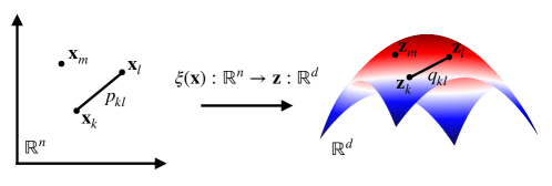
To reduce the dimensionality of the high-dimensional space and obtain a more useful representation with a lower number of degrees of freedom, we map the configuration variables to a limited number of functions of the configuration variables, or so-called CVs. A corresponding target mapping $\xi$ is the following:

$$\mathbf{x}\mapsto\xi(\mathbf{x})\equiv\big{\{}\xi_{k}(\mathbf{x})\big{\}}_{k=1}^{d},$$ (2)

where $d$ is the number of CVs ($d\ll n$) and $\{\xi_{k}\}$ are CVs.

The parametrization of the target mapping is performed to retain the system characteristics after embedding into the low-dimensional CV space (Fig. 1). In contrast to the configuration variables $\mathbf{x}$, there are several requirements that the optimal CVs should fulfill, i.e., ($i$) they should be few in number (i.e., the CV space should be low-dimensional), ($ii$) they should correspond to slow modes of the system, and ($iii$) they should separate relevant metastable states. If these requirements are met, we can quantitatively describe rare events.

Figure 1: Target mapping from high-dimensional samples of configuration variables $\mathbf{x}$ to a low-dimensional manifold spanned by CVs $\mathbf{z}$. In our framework, learning CVs is equivalent to finding the optimal parametrization of the target mapping $\mathbf{z}=\xi(\mathbf{x})$ [Eq. (2)]. The target mapping performs the reduction from $\mathbb{R}^{n}$ to $\mathbb{R}^{d}$ so the relation $p_{kl}$ between the high-dimensional samples $\mathbf{x}_{k}$ and $\mathbf{x}_{l}$ is preserved in the relation $q_{kl}$ in a low-dimensional manifold between the CV samples $\mathbf{z}_{k}$ and $\mathbf{z}_{l}$. For a detailed discussion, see Secs. II.5 and III.2.

Let us assume the target mapping and the CVs are known. Then, we can calculate the equilibrium marginal distribution of CVs by integrating over other variables:

$$P(\mathbf{z})=\int\operatorname{d\mathbf{x}}\delta\left(\mathbf{z}-\xi(\mathbf{x})\right)P(\mathbf{x}),$$ (3)

where the $\delta$-distribution is $\delta(\mathbf{z}-\xi(\mathbf{x}))=\prod_{k}\delta(z_{k}-\xi_{k}(\mathbf{x}))$.

Having the marginal equilibrium probability, we can define the free-energy landscape in the CV space as the negative logarithm multiplied by the thermal energy:

$$F(\mathbf{z})=-\frac{1}{\beta}\log P(\mathbf{z}).$$ (4)

In practice, free-energy landscapes for systems severely affected by the sampling problem are characterized by many metastable states separated by high kinetic barriers that impede transitions between metastable states. Consequently, on the timescales we can simulate, the system stays kinetically trapped in a single free-energy minimum and cannot explore the CV space efficiently.

II.2 Enhanced Sampling

CV-based enhanced sampling techniques overcome the sampling problem by introducing a bias potential $V(\mathbf{z})$ acting in the CV space designed to enhance CV fluctuations. The functional form of the bias depends on the enhanced sampling method used Torrie and Valleau (1977); Laio and Parrinello (2002); Barducci et al. (2008); Valsson and Parrinello (2014); Valsson et al. (2016); Hénin et al. (2022). The bias potential can be static Torrie and Valleau (1977) or adaptively constructed on the fly during the simulation Laio and Parrinello (2002); Barducci et al. (2008); Valsson and Parrinello (2014); Valsson et al. (2016); Hénin et al. (2022). Regardless of how the bias potential is constructed, it leads to a biased CV distribution that is smoother and easier to sample than the unbiased distribution [Eq. (3)]:

$$P_{V}(\mathbf{z})=\Big{\langle}\delta\left(\mathbf{z}-\xi(\mathbf{x})\right)\Big{\rangle}_{V}=\frac{1}{\mathcal{Z}_{V}}\operatorname{e}^{-\beta\left(F(\mathbf{z})+V(\mathbf{z})\right)},$$ (5)

where $\left\langle\cdot\right\rangle_{V}$ denotes the biased ensemble average and the biased partition function is $\mathcal{Z}_{V}=\int\operatorname{d\mathbf{z}}\operatorname{e}^{-\beta\left(F(\mathbf{z})+V(\mathbf{z})\right)}$.

CV-based enhanced sampling methods construct the bias potential to reduce or entirely flatten free-energy barriers. Let us consider well-tempered metadynamics Barducci et al. (2008), which is the method we employ in this work. Well-tempered metadynamics uses a history-dependent bias potential updated iteratively by periodically depositing Gaussians centered at the current location in the CV space. The bias potential is given as:

$$V(\mathbf{z})=\sum_{l}G_{\sigma}(\mathbf{z},\mathbf{z}_{l})\exp\left(-\frac{1}{\gamma-1}\beta V(\mathbf{z}_{l})\right),$$ (6)

where $G_{\sigma}(\mathbf{z},\mathbf{z}_{l})$ is a Gaussian kernel with a bandwidth set $\sigma$, $\mathbf{z}_{l}$ is the center of $l$-th added Gaussian, and $\gamma$ is a bias factor that determines how much we enhance CV fluctuations. Well-tempered metadynamics convergences to a biased CV distribution given by the so-called well-tempered distribution:

$$P_{V}(\mathbf{z})=\frac{\left[P(\mathbf{z})\right]^{1/\gamma}}{\int\operatorname{d\mathbf{z}}\,\left[P(\mathbf{z})\right]^{1/\gamma}},$$ (7)

which we can view as sampling an effective free-energy landscape $F/\gamma$ with barriers reduced by a factor of $\gamma$.

II.3 Reweighting

Biasing results in gradual diverging from the equilibrium CV distribution to a smoother and easier to sample biased CV distribution, i.e., from Eq. (3) to Eq. (7) in the case of well-tempered metadynamics. Consequently, the importance of each sample is given by a statistical weight needed to account for the effect of the bias potential when obtaining equilibrium properties such as the free-energy landscape. This contrasts with unbiased simulations where samples are equally important as they are sampled according to the equilibrium distribution.

A functional form of the weights depends on a particular method. Generally, for methods employing a bias potential $V(\mathbf{z})$, the weight associated with a CV sample $\mathbf{z}$ can be written as:

$$w(\mathbf{z})=\operatorname{e}^{\beta V(\mathbf{z})}.$$ (8)

In the case of a static bias, the weights are given by Eq. (8). In contrast, well-tempered metadynamics uses an adaptive bias potential [Eq. (6)], and we need to account for a time-dependent constant given by Tiwary and Parrinello (2015); Valsson et al. (2016):

$$c=\frac{1}{\beta}\log\frac{\int\operatorname{d\mathbf{z}}\exp\left(\frac{\gamma}{\gamma-1}\beta V(\mathbf{z})\right)}{\int\operatorname{d\mathbf{z}}\exp\left(\frac{1}{\gamma-1}\beta V(\mathbf{z})\right)},$$ (9)

which is independent of $\mathbf{z}$. We can then redefine the weights as:

$$w(\mathbf{z})=\operatorname{e}^{\beta(V(\mathbf{z})+c)},$$ (10)

where $V(\mathbf{z})+c$ is called the relative bias potential.

Note that in the above discussion, we assume that the dependence of the bias potential on the simulation time is implicit. We can ignore the time dependence once the simulation reaches convergence, then the relative bias potential $V(\mathbf{z})+c$ is quasi-stationary and does not change considerably (the bias potential $V(\mathbf{z})$ and the time-dependent constant $c$ can still increase while their sum converges). In practice, when performing reweighting, we ignore a short initial transient part of the simulation where the relative bias potential is still changing considerably.

The standard reweighting works by employing the weights to obtain the stationary equilibrium distribution from the biased CV distribution, i.e., $P(\mathbf{z})\propto w(\mathbf{z})P_{V}(\mathbf{z})$. The unbiased probability distribution $P(\mathbf{z})$ can be computed by histogramming or kernel density estimation, where each sample $\mathbf{z}$ is weighted by Eq. (8). This is done routinely in advanced simulation codes, e.g., plumed Tribello et al. (2014); plumed Consortium (2019).

Manifold learning methods cannot use the standard reweighting to unbias pairwise relations between samples. Instead, a non-trivial approach to reweighting in a form of $r(\mathbf{x}_{k},\mathbf{x}_{l})$ is required, where $r(\mathbf{x}_{k},\mathbf{x}_{l})$ is a pairwise reweighting factor that characterizes the importance of relation between samples $\mathbf{x}_{k}$ and $\mathbf{x}_{l}$.

II.4 Biased Data for Manifold Learning

Given the requirements for the optimal CVs (Sec. II.1), it is non-trivial to provide low-dimensional CVs knowing only the microscopic coordinates. Instead, we often resort to an intermediate description and select a large set of the configuration variables (often called features). For example, this might be internal coordinates such as distances or dihedral angles, and so forth. These configuration variables then define a high-dimensional space which we reduce to the optimal low-dimensional CVs. For a list of helpful configuration variables to characterize different physical systems, see, for example, the plumed documentation plu .

Consider data obtained from enhanced sampling simulations in which we record or select samples of the high-dimensional configuration variables $\mathbf{x}$. These data define the training set from which manifold learning methods construct a low-dimensional manifold. The training data set can be generally expressed as:

$$D_{V}=\Big{\{}(\mathbf{x}_{k}\in\mathbb{R}^{n},w(\mathbf{x}_{k}))\Big{\}}_{k=1}^{K},$$ (11)

where $K$ is the number of samples and the sample set is augmented by the corresponding statistical weights. Note that the weights depend on $\mathbf{x}$ through the CV mapping [Eq. (2)].

II.5 Diffusion Reweighting

Geometrically, the existence of a low-dimensional representation assumes that the high-dimensional dynamical system populates a low-dimensional manifold. This assumption is known as the manifold hypothesis Ferguson et al. (2011b). Under this view, the fast degrees of freedom are adiabatically slaved to the dynamics of the slow degrees of freedom, which correspond to the optimal CVs, due to the presence of fast equilibration within the metastable states. Methods leveraging this assumption belong to a class of manifold learning techniques.

The core of manifold learning methods appropriate for dimensionality reduction in dynamical systems is the construction of a random walk through a Markov chain on the data set, where the transition probabilities $p_{kl}$ depend on a kernel function and distances between samples. Depending on how the transition probabilities $p_{kl}$ are used to find a target mapping to a low-dimensional manifold, we can distinguish two main approaches: ($i$) eigendecomposition Molgedey and Schuster (1994); Roweis and Saul (2000); Tenenbaum et al. (2000); Belkin and Niyogi (2003); Coifman et al. (2005); Nadler et al. (2006); Coifman and Lafon (2006); Coifman et al. (2008); Tiwary and Berne (2016) and ($ii$) divergence optimization Hinton and Roweis (2002); van der Maaten and Hinton (2008); McInnes et al. (2018). In manifold learning methods using eigendecomposition, eigenvalues and eigenvectors are used to construct the target mapping. In methods employing divergence optimization, however, the transition probabilities $p_{kl}$ are used to find a Markov transition matrix $q_{kl}$ constructed from low-dimensional samples (Fig. 1).

Although many kernels can be considered in manifold learning, a typical choice in spectral embedding methods is a Gaussian kernel dependent on Euclidean distances Belkin and Niyogi (2001); Coifman et al. (2005):

$$p_{kl}\sim G_{\varepsilon}(\mathbf{x}_{k},\mathbf{x}_{l})=\exp\left(-\frac{1}{\varepsilon}\|\mathbf{x}_{k}-\mathbf{x}_{l}\|^{2}\right),$$ (12)

where $\varepsilon$ is a positive parameter chosen depending on the given data set as it induces a length scale ${\sim}\sqrt{\varepsilon}$ that should match the distance between neighboring samples. Eq. (12) models the Markov transition matrix if every row is normalized to unity.

However, this construction includes information only on the manifold geometry given by the pairwise distances. The remaining components required for our reweighting approach are the density and importance of the data.

For the Markov transition matrix, the reweighting procedure must be reformulated to include the weights $w(\mathbf{x}_{k})$ and $w(\mathbf{x}_{l})$ for a pair of samples $\mathbf{x}_{k}$ and $\mathbf{x}_{l}$, respectively. Our plan is to derive such a pairwise reweighting formula where each pairwise transition probability given by the Markov transition matrix $M(\mathbf{x}_{k},\mathbf{x}_{l})$ depends also on a reweighting factor $r(\mathbf{x}_{k},\mathbf{x}_{l})$. We assume that a reweighted Markov transition matrix can be defined in a simple form:

$$M(\mathbf{x}_{k},\mathbf{x}_{l})\propto r(\mathbf{x}_{k},\mathbf{x}_{l})G_{\varepsilon}(\mathbf{x}_{k},\mathbf{x}_{l}),$$ (13)

where $M$ is row-stochastic. The Markov transition matrix models then the unbiased Markov chain where each entry is the probability of the jump from $\mathbf{x}_{k}$ to $\mathbf{x}_{l}$.

To account for the manifold density, we need to employ a density-preserving kernel. In contrast to Laplacian eigenmaps that are appropriate for data sampled uniformly Belkin and Niyogi (2001, 2003), diffusion map allows working with data sampled from any underlying probability distribution. Specifically, let us consider the pairwise transition probabilities based on an anisotropic diffusion kernel given by Coifman et al. (2005):

$$\kappa(\mathbf{x}_{k},\mathbf{x}_{l})=\frac{G_{\varepsilon}(\mathbf{x}_{k},\mathbf{x}_{l})}{[\rho(\mathbf{x}_{k})]^{\alpha}[\rho(\mathbf{x}_{l})]^{\alpha}},$$ (14)

where $\rho(\mathbf{x})$ is a kernel density estimator and $\alpha\in[0,1]$ is the anisotropic diffusion parameter, which is crucial to properly include information about the data density and importance Nadler et al. (2006). Based on the anisotropic diffusion parameter, diffusion map can be used to parametrize a family of low-dimensional embeddings.

In Eq. (14), the density estimator $\rho(\mathbf{x}_{k})$ at a sample $\mathbf{x}_{k}$ must be reweighted to account on the data importance:

$$\rho(\mathbf{x}_{k})=\sum_{l}w(\mathbf{x}_{l})G_{\varepsilon}(\mathbf{x}_{k},\mathbf{x}_{l}),$$ (15)

which is a weighed kernel density estimate up to an unimportant multiplicative constant. After the reweighting, the density estimator characterizes the unbiased density, in contrast to the biased density estimate that is given as:

$$\rho_{V}(\mathbf{x}_{k})=\sum_{l}G_{\varepsilon}(\mathbf{x}_{k},\mathbf{x}_{l}),$$ (16)

where the subscript $V$ denotes that the density estimate is calculated under the bias potential $V$.

In theory, if the underlying probability distribution of high-dimensional samples is known analytically, it is possible to express $\rho$ directly from this distribution Coifman et al. (2008); e.g., from a Boltzmann distribution [Eq. (1)] if the samples are represented by the microscopic coordinates. However, this is valid only in the case of sufficient sampling and thus rarely reachable in practice. Moreover, the high-dimensional distribution $P(\mathbf{x})$ of the configuration variables is unknown in general (Sec. II.1). For this reason, we write $\rho$ as a kernel density estimate [Eq. (15)].

We can understand the physical meaning behind the anisotropic diffusion kernel by considering Eq. (14). The dynamics described by Eq. (14) is local as samples closer to each other have a higher probability of being close in the respective low-dimensional manifold and vice versa in the case that they are farther apart. This information about the underlying geometry is given by $G_{\varepsilon}(\mathbf{x}_{k},\mathbf{x}_{l})$ which requires that the transition probabilities are penalized between geometrically distant samples $\mathbf{x}_{k}$ and $\mathbf{x}_{l}$. The density and importance of samples are encoded in the unbiased density estimates [Eq. (15)].

Depending on $\alpha$ value in Eq. (14), three interesting cases of diffusion maps can be considered asymptotically Nadler et al. (2006). Namely, ($i$) for $\alpha=\frac{1}{2}$, Eq. (14) corresponds to the Markov chain that is an approximation of the diffusion given by the Fokker-Planck generator with the underlying data density proportional to the equilibrium density, allowing us to approximate the long-time behavior of the microscopic coordinates. Other values of $\alpha$ are also possible, e.g., ($ii$) for $\alpha=0$, we get the classical normalized graph Laplacian, and ($iii$) for $\alpha=1$, we ignore the underlying density and the diffusion operator approximates the Laplace-Beltrami operator. We note that this asymptotic behavior holds in the limit of infinite data $K\rightarrow\infty$ and $\varepsilon\rightarrow 0$ when considering the microscopic coordinates. As we are interested in finding low-dimensional CVs, the case for $\alpha=\frac{1}{2}$ is appropriate to model asymptotically the slowest degrees of freedom, accounting for both the underlying geometry and density of the manifold.

As we have all the required ingredients for the reweighting of Markov transition matrices, we focus on deriving the reweighting factor. Here, we discuss only an outline, while a detailed derivation is provided in Appendix A.

Based on Eq. (14), the Markov transition matrix can be estimated by weighting each Gaussian term and normalizing it so that it is row-stochastic:

$$M(\mathbf{x}_{k},\mathbf{x}_{l})=\frac{w(\mathbf{x}_{l})\kappa(\mathbf{x}_{k},\mathbf{x}_{l})}{\sum_{m}w(\mathbf{x}_{m})\kappa(\mathbf{x}_{k},\mathbf{x}_{m})}.$$ (17)

Next, by inserting Eq. (14) to Eq. (17), we can see that the Markov transition matrix $M$ can be written also using the Gaussian kernels:

$$M(\mathbf{x}_{k},\mathbf{x}_{l})\propto\frac{w(\mathbf{x}_{k})}{{[\rho(\mathbf{x}_{k})]^{\alpha}}}\frac{w(\mathbf{x}_{l})}{{[\rho(\mathbf{x}_{l})]^{\alpha}}}G_{\varepsilon}(\mathbf{x}_{k},\mathbf{x}_{l}),$$ (18)

where we can recognize the reweighting factor by comparing the result to Eq. (13). Therefore, we get the following expression:

$$r(\mathbf{x}_{k},\mathbf{x}_{l})=\frac{w(\mathbf{x}_{k})}{{[\rho(\mathbf{x}_{k})]^{\alpha}}}\frac{w(\mathbf{x}_{l})}{{[\rho(\mathbf{x}_{l})]^{\alpha}}}.$$ (19)

We can also approximate the reweighting factor by rewriting Eq. (19) with the biased density estimate [Eq. (16)]:

$$r(\mathbf{x}_{k},\mathbf{x}_{l}) =\frac{w(\mathbf{x}_{k})}{\sqrt{\rho(\mathbf{x}_{k})}}\frac{w(\mathbf{x}_{l})}{\sqrt{\rho(\mathbf{x}_{l})}}$$

$$\approx\frac{w(\mathbf{x}_{k})}{\sqrt{w(\mathbf{x}_{k})\rho_{V}(\mathbf{x}_{k})}}\frac{w(\mathbf{x}_{l})}{\sqrt{w(\mathbf{x}_{l})\rho_{V}(\mathbf{x}_{l})}}$$

$$=\sqrt{\frac{w(\mathbf{x}_{k})}{\rho_{V}(\mathbf{x}_{k})}}\sqrt{\frac{w(\mathbf{x}_{l})}{\rho_{V}(\mathbf{x}_{l})}},$$ (20)

where we set $\alpha=\frac{1}{2}$. Eq. (II.5) is a final form of the reweighting factor that we use here. A detailed derivation of Eq. (II.5) is provided in Appendix A. Although the derivation of Eq. (II.5) is presented using the Gaussian kernel, our framework can be used in other manifold learning methods, as demonstrated in Sec. III.

Eq. (18) denotes an unbiased Markov chain with the transition probability from $\mathbf{x}_{k}$ to $\mathbf{x}_{l}$ in one time step $t$ given by:

$$\mathrm{Pr}\big{\{}\mathbf{x}(t+1)=\mathbf{x}_{l}\,|\,\mathbf{x}(t)=\mathbf{x}_{k}\big{\}}=M(\mathbf{x}_{k},\mathbf{x}_{l}).$$ (21)

We term our reweighting procedure diffusion reweighting. We postulate that the derived Markov transition matrix [Eq. (18)] has the following three properties that make the construction of Eq. (21) from enhanced sampling simulations feasible. Namely, the Markov transition matrix encodes the information about:

1. Geometry $G_{\varepsilon}(\mathbf{x}_{k},\mathbf{x}_{l})$: The probability of transitions between samples lying far from each other is low and high for those in close proximity.

2. Density $[\rho(\mathbf{x}_{l})]^{\alpha}$: The anisotropic diffusion constant $\alpha\in[0,1]$ is used as a density-scaling term as in diffusion maps. See Eq. (14) and the corresponding description.

3. Importance $w(\mathbf{x}_{l})$: The statistical weights from enhanced sampling decide accordingly to the bias if a sample is important, i.e., metastable states where the weights are higher are more important then high free-energy regions.

II.6 Implementation

Our framework is implemented in a development version of plumed 2.7 Tribello et al. (2014); plumed Consortium (2019) as the LowLearner module and will be made publicly available in the coming future.

III Reweighted Manifold Learning

We incorporate diffusion reweighting into several manifold learning methods and apply them to find a low-dimensional representation in a model system and high-dimensional atomistic simulation problems represented by biased simulation data. Specifically, we consider diffusion reweighting in diffusion maps Nadler et al. (2006); Coifman and Lafon (2006); Coifman et al. (2008) and recently introduced stochastic embedding methods for learning CVs and adaptive biasing Zhang and Chen (2018); Rydzewski and Valsson (2021).

To demonstrate the validity of our framework, we apply diffusion map to standard testing systems such as a particle moving on an analytical potential and alanine dipeptide. For the stochastic embedding methods, we choose a mini-protein chignolin. For the two atomistic systems, alanine dipeptide and chignolin, we describe the systems using two different types of high-dimensional representations (distances and dihedral angles, respectively) to show that the framework can work regardless of the chosen configuration variables.

III.1 Diffusion Maps

We start by considering the case of diffusion maps on which we base the derivation of the reweighting factor $r(\mathbf{x}_{k},\mathbf{x}_{l})$ (Sec. II.5). By rewriting the diffusion kernel using the biased density estimates [Eq. (II.5)], we can use it to construct a low-dimensional embedding from a biased data set. We directly use Eq. (18) to estimate the transition probabilities while using Eq. (II.5) to account for the sampling from any biased distribution.

III.1.1 Target Mapping $\xi(\mathbf{x})$: Eigendecomposition

With the exemption of the reweighting factor, further steps in our approach to diffusion maps proceed as in its standard formulation Nadler et al. (2006). Let us briefly recap these steps.

In diffusion maps, the spectral decomposition of the Markov transition matrix $M$ is performed to define a low-dimensional embedding, $M\psi=\lambda\psi$, where $\{\lambda_{l}\}$ and $\{\psi_{l}\}$ are eigenvalues and eigenvectors, respectively. The eigenvalues are related to the effective timescales as $\tau_{l}=-\frac{1}{\log\lambda_{l}}$ and can be used to determine the slowest processes in the dynamics. Then, the eigenvectors corresponding to the largest eigenvalues define a reduced space. Given this interpretation, the target mapping [Eq. (2)] is defined by the diffusion coordinates:

$$\xi(\mathbf{x})=\big{\{}\lambda_{k}\psi_{k}(\mathbf{x})\big{\}}_{k=0}^{d-1},$$ (22)

where $\xi(\mathbf{x})$ is computed using the first $d$ eigenvalues and eigenvectors with the the equilibrium density represented by the zeroth coordinate $\lambda_{0}\psi_{0}$. In Eq. (22), the spectrum of the eigenvalues $\{\lambda_{l}\}$ is sorted by non-increasing value, $\lambda_{0}=1>\lambda_{1}\geq\dots\geq\lambda_{d-1}$.

The truncation up to $d-1$ of Eq. (22) for metastable systems corresponds to a negligible error on the order of $O(\lambda_{d}/\lambda_{d-1})$ Nadler et al. (2006). In other words, this assumption relates to a large spectral gap that separates slow degrees of freedom ($>\lambda_{d-1}$) and fast degrees of freedom ($<\lambda_{d-1}$). For a detailed description behind the construction of the diffusion coordinates, we refer to works by Coifman Coifman et al. (2005); Coifman and Lafon (2006); Coifman et al. (2008).

III.1.2 Algorithm

The described algorithm for our reweighted diffusion maps is given in Algorithm 1.

Input : Biased data set $\big{\{}(\mathbf{x}_{k},w(\mathbf{x}_{k}))\big{\}}_{k=1}^{K}$.

Output : Eigenvalues $\{\lambda_{k}\}$ and eigenvectors $\{\psi_{k}\}$ of the transition matrix $M$ used to construct the target mapping $\xi$.

1. Calculate the squared pairwise distances $\|\mathbf{x}_{l}-\mathbf{x}_{l}\|^{2}$.

2. Estimate the Markov transition matrix $M(\mathbf{x}_{k},\mathbf{x}_{l})$:

   1. Apply the Gaussian kernel $G_{\varepsilon}(\mathbf{x}_{k},\mathbf{x}_{l})$ [Eq. (12)].

   2. Construct the anisotropic diffusion kernel using the reweighting factor $r(\mathbf{x}_{k},\mathbf{x}_{l})$ [Eq. (II.5)].

   3. Normalize to obtain the row-stochastic matrix $M$.

3. Perform eigendecomposition $M\psi=\lambda\psi$ and estimate the diffusion coordinates $\xi(\mathbf{x})$ [Eq. (22)].

Algorithm 1 Reweighted Diffusion Maps

III.1.3 Example: Model Potential

As a simple and illustrative example of applying diffusion reweighting within the diffusion map framework, we consider a case where dimensionality reduction is not performed. Namely, we run an enhanced sampling simulation of a single particle moving along the $x$ variable on a one-dimensional potential $U(x)$ with three Gaussian-like metastable states with different energy depths and energy barriers between the minima [Fig. 2($a$)]. In this system, the highest energy barrier is ${\sim}50~{}k_{\mathrm{B}}T$, which makes the transitions from the deepest minimum rare. The dynamics is modeled by a Langevin integrator Bussi and Parrinello (2007) using temperature $T=1$, a friction coefficient of 10, and a time step of 0.005. We employ the pesmd code in the plumed Tribello et al. (2014); plumed Consortium (2019) plugin. We bias the $x$ variable using well-tempered metadynamics Barducci et al. (2008) with a bias factor of $\gamma=10$. Further details about the simulation are given in Supplemental Material sm .

Figure 2: Diffusion maps generated for the reweighted and non-reweighted (without applying diffusion reweighting) biased simulation of a particle in a simple ($a$) one-dimensional potential $U(x)$ where the energy barriers separating the deepest minimum are on the order of 50 $k_{\mathrm{B}}T$, and the corresponding transitions from this state are rare events. ($b$) A comparison between the non-reweighted (blue) and reweighted (red) diffusion maps: the equilibrium densities along the coordinate $x$ and diffusion coordinates $\lambda_{0}\psi_{0}$ vs. $\lambda_{1}\psi_{1}$, with coloring according to the $x$ value. The enhanced sampling simulation is performed using well-tempered metadynamics Barducci et al. (2008) with a bias factor of 10 by employing the pesmd code in the plumed Tribello et al. (2014); plumed Consortium (2019) plugin.

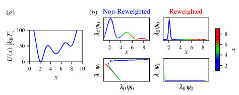
We present our results in Fig. 2($b$). We can see that the non-reweighted (without applying diffusion reweighting) diffusion map learns the biased distribution (given by $\lambda_{0}\psi_{0}$) along the coordinate $x$ where the three energy minima correspond to the maxima of the biased distribution. Additionally, the first two diffusion coordinates are not orthogonal, and there is a lack of separation between the metastable states.

In contrast, the reweighted diffusion map can represent the equilibrium density ($\lambda_{0}\psi_{0}$) where only the first energy minimum is populated due to the high-free energies separating the states. The $\lambda_{0}\psi_{0}$ and $\lambda_{1}\psi_{1}$ diffusion coordinates properly separate the samples. We can see that $\lambda_{1}\psi_{1}$ is almost marginal due to the lack of additional dimensions for the potential energy.

The example presented in Fig. 2 is, of course, a trivial case in which no dimensionality reduction is performed; however, it indicates that diffusion reweighting can be used to reweight the transition probabilities successfully and that the standard diffusion map trained on the biased data captures an incorrect representation.

III.1.4 Example: Alanine Dipeptide

Figure 3: Reweighted diffusion maps on a peptide model system (Ace-Ala-Nme) in vacuum at 300 K simulated using well-tempered metadynamics Barducci et al. (2008) enhancing the $\Phi$ and $\Psi$ dihedral angles and a bias factor $\gamma=5$. The diffusion map is calculated using a high-dimensional space of 45 pairwise distances between heavy atoms. ($a$) A representative structure of alanine dipeptide with the dihedral angles $\Phi$ and $\Psi$. ($b$) A spectrum of eigenvalues $\{\lambda_{l}\}$ obtained from the eigendecomposition for the non-reweighted (blue) and reweighted (red) Markov transition matrices. ($c$) The samples are shown in the dihedral angle space for the non-reweighted (blue label) and reweighted (red label) diffusion map with colors representing the first and second diffusion-map coordinates $\lambda_{0}\psi_{0}(\mathbf{x})$ and $\lambda_{1}\psi_{1}(\mathbf{x})$, respectively. The color bar represents the constructed diffusion coordinates.

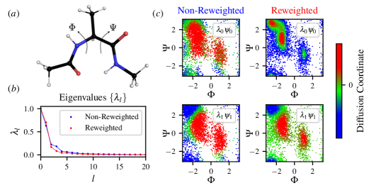
As a next example, we consider alanine dipeptide (Ace-Ala-Nme) in gas phase described using the Amber99-SB force field Hornak et al. (2006). The data set is generated by a 100-ns molecular dynamics simulation Bussi et al. (2007); Hess (2008) using the gromacs 2019.2 code Abraham et al. (2015) patched with a development version of the plumed Tribello et al. (2014); plumed Consortium (2019) plugin. The simulation is performed by well-tempered metadynamics Barducci et al. (2008) at 300 K using the backbone dihedral angles $\Phi$ and $\Psi$ for biasing and a bias factor of 5. Using this setup, the convergence of the bias potential is obtained fairly quickly. Further details about the simulation are given in Supplemental Material sm .

Using diffusion maps, we reduce the high-dimensional space consisting of all pairwise distances between the heavy atoms ($n=45$) to two dimensions. The diffusion maps are constructed using $\varepsilon=0.078$ estimated as the median of the pairwise distances.

We present diffusion reweighting results for alanine dipeptide in Fig. 3. The eigenvalues of the Markov transition matrix have a spectral gap (i.e., timescale separation) with only a few eigenvalues close to one and all other eigenvalues much smaller than one. Thus, only the first few eigenvectors are needed to approximate the diffusion coordinates [Eq. (22)] and thus the target mapping to the CV space. The eigenvalues $\{\lambda_{l}\}$ indicate that the spectral gap is slightly wider for the reweighted transition probability matrix, as can be seen in Fig. 3($b$). Consequently, the effective timescales $\tau_{l}=-\frac{1}{\log\lambda_{l}}$ calculated from the eigenvalues indicate that the reweighted diffusion map corresponds to slower processes; see Supplemental Material sm .

We can see that the non-reweighted approach cannot correctly account for the transition probabilities calculated based on the biased simulation, as we expected. The transitions between the metastable states are so frequent that the first diffusion coordinate (the equilibrium density) suggests only one metastable state [Fig. 3($c$)]. In Supplemental Material sm , we show that the separation of samples in the reweighted diffusion map is much better than for the non-reweighted diffusion map. It resembles a “typical” diffusion map from unbiased data sets.

In the reweighted case, the low-dimensional coordinates can distinguish between the relevant metastable states. Additionally, using Eq. (II.5) the first diffusion-map coordinate, $\lambda_{0}\psi_{0}(\mathbf{x})$, correctly encodes the information about the Boltzmann equilibrium distribution of alanine dipeptide in the dihedral angle space, which is not possible using the standard (i.e., non-reweighted) diffusion map in the case of biased simulation data [Fig. 3($c$)]. By comparing the reweighted diffusion map to a diffusion map constructed from an unbiased parallel tempering replica at 300 K, we can see that the embeddings and eigenvalues are virtually identical; see Supplemental Material sm .

These results further corroborate our findings and show that when performing a dimensionality reduction from data resulting from enhanced sampling, the reweighting factor [Eq. (II.5)] is needed to revert the effect of biasing in the transition probability matrix.

III.2 Stochastic Embeddings

Next, we move to employ diffusion reweighting in more recent approaches. We consider manifold learning methods devised primarily to learn CVs from biased simulation trajectories: multiscale reweighted stochastic embedding (mrse) Rydzewski and Valsson (2021) and stochastic kinetic embedding (stke) Zhang and Chen (2018). These methods use approximations of the reweighting factor [Eq. (II.5)]. Our aim is not to compare results obtained using these methods but to present and discuss how diffusion reweighting can be approximated and employed in manifold learning methods other than diffusion maps.

First, let us focus on a general procedure these stochastic embedding methods use to parametrize manifolds. Mainly, we discuss how these methods use the Markov transition matrices to parametrize the target mapping to low-dimensional manifolds. The construction of the Markov transition matrix with reweighting from biased data in each technique is discussed in the remainder of this section.

III.2.1 Target Mapping $\xi_{\boldsymbol{\theta}}(\mathbf{x})$: Divergence Optimization

As mentioned above, the stochastic embedding methods belong to the second category of manifold learning methods we consider here, i.e., based on divergence optimization. Thus, unlike diffusion maps, the eigendecomposition is not performed in these methods. Instead, the target mapping $\xi$ is parametrized based on neural networks that perform nonlinear dimensionality reduction. The target mapping is given as:

$$\mathbf{z}:\mathbf{x}\mapsto\xi_{\boldsymbol{\theta}}(\mathbf{x}),$$ (23)

where $\boldsymbol{\theta}=\{\theta_{k}\}$ are parameters of the target mapping adjusted such that the low-dimensional manifold of CVs is optimal with respect to a selected statistical measure. Using Eq. (23), the distance between samples in a manifold can be given as:

$$\|\mathbf{z}_{k}-\mathbf{z}_{l}\|=\|\xi_{\boldsymbol{\theta}}(\mathbf{x}_{k})-\xi_{\boldsymbol{\theta}}(\mathbf{x}_{l})\|.$$ (24)

Note that in some simple cases, the mapping in Eq. (23) can also be represented using a linear combination. However, deep learning has been successful in a broad range of learning problems, and using more intricate approximations for the mapping between high-dimensional and low-dimensional spaces is quite common for complex data sets Hinton and Salakhutdinow (2006); van der Maaten (2009).

The target mapping is parametrized by comparing the Markov transition matrix $M(\mathbf{x}_{k},\mathbf{x}_{l})=(p_{kl})$ (Sec. III.2.2) constructed from the high-dimensional samples to a Markov transition matrix $Q(\mathbf{z}_{k},\mathbf{z}_{l})=(q_{kl})$ built from low-dimensional samples mapped using the target mapping [Eq. (23)]. In stke, we use a Gaussian kernel for $Q$:

$$q_{kl}\sim\exp\left(-\frac{1}{\varepsilon}\|\xi_{\boldsymbol{\theta}}(\mathbf{x}_{k})-\xi_{\boldsymbol{\theta}}(\mathbf{x}_{l})\|^{2}\right).$$ (25)

In mrse, we employ a one-dimensional $t$-distribution, as implemented in $t$-sne van der Maaten and Hinton (2008); van der Maaten (2009). Taking the target mapping as defined in Eq. (23), the transition probabilities in the low-dimensional space $q_{kl}$ in mrse are:

$$q_{kl}\sim\big{(}1+\|\xi_{\boldsymbol{\theta}}(\mathbf{x}_{k})-\xi_{\boldsymbol{\theta}}(\mathbf{x}_{l})\|^{2}\big{)}^{-1}.$$ (26)

The choice of the $t$-distribution for $Q$ in mrse is motivated by the apparent crowding problem van der Maaten and Hinton (2008), i.e., as the volume of a small-dimensional neighborhood grows slower than the volume of a high-dimensional one, the neighborhood is stretched so that moderately distant sample pairs are placed too far apart. As outlined in Refs. van der Maaten and Hinton (2008), the use of a heavy-tailed distribution for the low-dimensional representation allows moderate distances in the high-dimensional space to be represented by much larger distances in the manifold, encouraging gaps to form in the low-dimensional map between the clusters present in the data, alleviating the crowding problem to some degree.

Finally, the Markov transition matrices computed from the high-dimensional and low-dimensional samples need to be compared. The most common choice for such a metric is employing a statistic distance, particularly the Kullback–Leibler divergence:

$$D_{\mathrm{KL}}(M,Q;\boldsymbol{\theta})=\sum_{k}\sum_{l}p_{kl}\log\frac{p_{kl}}{q_{kl}},$$ (27)

where in contrast to the standard formulation of the Kullback–Leibler divergence that compares two probability distributions, Eq. (27) is computed for every pair of rows from $M$ and $Q$, and then summed. There are many choices possible for the comparison between $M$ and $Q$, e.g., cross-entropy McInnes et al. (2018); Shires and Pickard (2021) or the Jensen–Shannon divergence Zhang and Chen (2018).

The Kullback–Leibler divergence optimization is performed to train the target mapping represented by a neural network. As the target mapping is parametric, the gradients of $D_{\mathrm{KL}}$ with respect to the parameters $\boldsymbol{\theta}=\{\theta_{k}\}$ of the neural network can be estimated effortlessly using backpropagation. For further details about training neural networks, we refer to Appendix E.

III.2.2 Reweighted Markov Transitions

After explaining how the parametric mapping is constructed in the reweighted stochastic embeddings, we proceed to formulate the Markov transition matrices and the reweighting factors for these methods.

First, let us consider the reweighting performed in mrse Rydzewski and Valsson (2021). This method employs the following reweighting factor:

$$r(\mathbf{x}_{k},\mathbf{x}_{l})=\sqrt{w(\mathbf{x}_{k})w(\mathbf{x}_{l})},$$ (28)

where we neglect the biased density estimates $\rho_{V}$ [cf. Eq. (28) and Eq. (II.5)]. The reweighting factor [Eq. (28)] written as a geometric mean between two statistical weights can be justified by the fact that the bias potential is additive, as shown in Eq. (8), and a geometric mean is appropriate to preserve this relation. We note that similar reweighting procedures have been used in Refs. Zheng et al. (2013b); Banisch et al. (2020); Trstanova et al. (2020).

The Markov transition matrix in mrse is expressed as a Gaussian mixture, where each Gaussian is evaluated for different $\varepsilon$ values and reweighted using Eq. (28):

$$M(\mathbf{x}_{k},\mathbf{x}_{l})\propto\sum_{\{\varepsilon\}}\sqrt{w(\mathbf{x}_{l})}G_{\varepsilon}(\mathbf{x}_{k},\mathbf{x}_{l}),$$ (29)

where we omit the normalization constant for brevity. The sum in Eq. (29) is over bandwidths that are automatically estimated and selected to fit that data. Note that many methods can be used for this purpose; however, to facilitate analysis, we use a method from Ref. Rydzewski and Valsson (2021). As this procedure is mostly technical, for details about estimating bandwidths and constructing the Gaussian mixture, we refer to Appendix C.

Second, let us consider stke. Suppose high-dimensional samples are resampled so that each sample keeps a certain distance away from the others. In that case, the distribution of samples can be viewed as approximately uniform. Then, $w(\mathbf{x})$ can be replaced by the unbiased probability density estimator $\rho(\mathbf{x})$ in Eq. (28). Thus, the reweighting factor is given by:

$$r(\mathbf{x}_{k},\mathbf{x}_{l})=\sqrt{\rho(\mathbf{x}_{k})\rho(\mathbf{x}_{l})},$$ (30)

which is the formula used in stke Zhang and Chen (2018); Chen (2021). The corresponding Markov transition matrix is:

$$M(\mathbf{x}_{k},\mathbf{x}_{l})\propto\sqrt{\rho(\mathbf{x}_{l})}G_{\varepsilon}(\mathbf{x}_{k},\mathbf{x}_{l}),$$ (31)

where, as in Eq. (29), the $k$-th reweighting term is canceled out during the normalization.

An interesting property of the transition probabilities used by this method is that by taking an approximation to the normalization constant (Appendix B), we arrive at a transition probability matrix of similar form as in the square-root approximation of the infinitesimal generator of the Fokker-Planck operator Lie et al. (2013); Heida (2018); Donati et al. (2018); Kieninger et al. (2020):

$$M(\mathbf{x}_{k},\mathbf{x}_{l})=\sqrt{\frac{\rho(\mathbf{x}_{l})}{\rho(\mathbf{x}_{k})}}G_{\varepsilon}(\mathbf{x}_{k},\mathbf{x}_{l}),$$ (32)

for a single $\varepsilon$. The square-root approximation has been initially derived by discretizing a one-dimensional Smoluchowski equation Bicout and Szabo (1998). It can also be shown that Eq. (32) can be obtained using the maximum path entropy approach Dixit (2019); Ghosh et al. (2020).

As many algorithmic choices are available for each procedure incorporated in the reweighted stochastic embedding framework, it is difficult to directly compare mrse and stke. However, we aim to discuss how approximations of the reweighting factor are employed in these methods and how they can be used to learn CVs from biased data. Thus, in the above discussion, we focus on the reweighting procedures for the Markov transition matrices used by these methods. To compare the parameters used by these methods, see Appendix E.

III.2.3 Algorithm

For a general algorithm used by the stochastic embedding techniques to find a low-dimensional manifold of data, see Algorithm 2.

Input : Biased data set $\big{\{}(\mathbf{x}_{k},w(\mathbf{x}_{k}))\big{\}}_{k=1}^{K}$.

Output : Target mapping $\mathbf{x}\mapsto\xi(\mathbf{x})$ and the CVs $\mathbf{z}$.

1. Calculate the squared pairwise distances $\|\mathbf{x}_{l}-\mathbf{x}_{l}\|^{2}$.

2. Estimate the Markov transition matrix $M(\mathbf{x}_{k},\mathbf{x}_{l})$ according to the method used and reweight $M$ using the approximation of the reweighting factor (Sec. III.2.2).

3. Use the target function $\xi_{\boldsymbol{\theta}}(\mathbf{x})$ to estimate parameters $\boldsymbol{\theta}=\{\theta_{k}\}$:

   1. Compute the transition matrix $Q(\mathbf{z}_{k},\mathbf{z}_{l})=(q_{kl})$ from the low-dimensional samples using the $t$-distribution as in mrse [Eq. (26)] or the Gaussian kernel as in stke [Eq. (25)].

   2. Use the Kullback-Leibler divergence $D_{\mathrm{KL}}(\boldsymbol{\theta})$ to estimate statistical distance between $Q$ and $M$ given the current parameters $\boldsymbol{\theta}$ [Eq. (27)].

   3. Repeat until convergence reached.

4. Map the high-dimensional samples to CVs using $\xi(\mathbf{x})$, where optimal parameters are given by $\operatorname*{arg\,min}D_{\mathrm{KL}}(\boldsymbol{\theta})$.

Algorithm 2 Reweighted Stochastic Embedding

III.2.4 Example: Chignolin

As an example for the two stochastic embedding methods mrse and stke, we consider folding and unfolding of a ten amino-acid miniprotein chignolin (CLN025) Honda et al. (2008) in the solvent. We employ the CHARMM27 force field Mackerell Jr et al. (2004) and the TIP3P water model Jorgensen et al. (1983), and we perform the molecular dynamics simulation Bussi et al. (2007); Hess (2008) using the gromacs 2019.2 code Abraham et al. (2015) patched with a development version of the plumed Tribello et al. (2014); plumed Consortium (2019) plugin. Our simulations are performed at 340 K for easy comparison with other simulation data, also simulated at 340 K Lindorff-Larsen et al. (2011); Palazzesi et al. (2017). We perform a 1-$\mu$s well-tempered metadynamics simulation with a large bias factor of 20. We select a high bias factor to illustrate that our framework is able to learn metastable states in a low-dimensional manifold even when free-energy barriers are virtually flattened, and the system dynamics is close to diffusive at convergence.

Figure 4: Reweighted stochastic embeddings calculated for chignolin in the TIP3P solvent at 340 K simulated using the CHARMM27 force field. Low-dimensional manifolds are colored according to their free energy. ($a$) Representative conformations from the metastable states estimated by the reweighted embedding methods are shown around the mrse embedding. ($b$) The embedding obtained using stke. Well-tempered metadynamics is used to generate the training set consisting of sines and cosines of all $\Phi$ and $\Psi$ dihedral angles, amounting to 32 variables in total. The training set is generated by performing a 1-$\mu$s simulation with a bias factor $\gamma=20$, enhancing the fluctuations of the distance $d$ between the C$\alpha$ atoms of residues Y1 and Y10 and the radius of gyration $r_{g}$. ($c$) The free-energy surface calculated along for $d$ and $r_{g}$. The axes and units for the embeddings are arbitrary and thus not shown. See Supplemental Material sm for computational details.

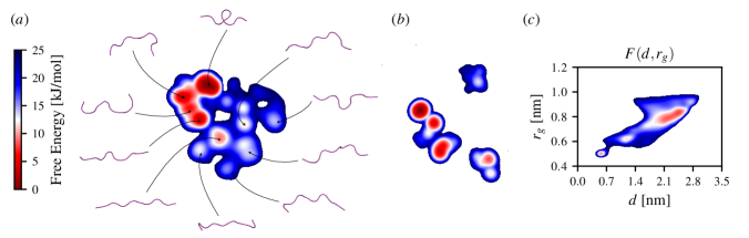
As biased CVs to enhance transitions between the folded and unfolded conformations of CLN025 in the metadynamics simulation, we choose the distance between C$\alpha$ atoms of residues Y1 and Y10 ($d$) and the radius of gyration ($r_{g}$) [Fig. 4($c$)]. We consider CLN025 conformations folded when the distance is below ${\sim}0.8$ nm and unfolded otherwise for $>0.8$ nm; see the corresponding time series in Supplemental Material sm . From the resulting trajectory, we calculate the sines and cosines of all the backbone $\Phi$ and $\Psi$ dihedral angles and use them as the high-dimensional representation of CLN025, which amounts to 32 variables in total. We collect high-dimensional samples every 1 ps for the biased training data set. Then, the low-dimensional manifolds are trained on representative samples selected as described in Refs. Zhang and Chen (2018); Rydzewski and Valsson (2021). As we focus mainly on the Markov transition matrices and diffusion reweighting here, we provide a detailed discussion about the subsampling procedures in Appendix D.

In Fig. 4, we present the resulting manifolds spanned by the trained CVs computed using the reweighted stochastic embedding methods (Sec. III.2). The embedding presented in Fig. 4($a$) is calculated using mrse Rydzewski and Valsson (2021), while the embedding presented in Fig. 4($b$) is calculated using stke Zhang and Chen (2018), using their corresponding reweighting formulas given by Eq. (28) and Eq. (30), respectively. For each manifold, the corresponding free-energy landscapes are calculated using kernel density estimation using the weights to reweight each sample [Eq. (10)].

We can observe that the free-energy landscape in the low-dimensional manifold calculated by mrse is highly heterogeneous, with multiple partially unfolded intermediate states and many possible reaction pathways, as shown in Fig. 4($a$). Such a complex free-energy landscape shows that the dynamics of CLN025 is more intricate and complex than it is visible in the free-energy surface spanned by the distance and the radius of gyration [Fig. 4($c$)], where we can see only the folded, intermediate, and unfolded states and remaining are possibly degenerate.

In Fig. 4, we can see the lower-lying free-energy basins in the reweighted stochastic embeddings are captured by both mrse and stke. We can also notice a slight difference between the metastable states lying higher in free energy. Specifically, mrse captures more states below a threshold of 25 kJ/mol in comparison to the embedding rendered by stke, in which the rest of the states is placed over 25 kJ/mol (i.e., mainly different unfolded states).

In our simulations, we do not observe a misfolded state of CLN025 shown to be highly populated in several studies Satoh et al. (2006); Lindahl et al. (2014) employing different force fields (Amber99 Wang et al. (2000) and Amber99-SB Hornak et al. (2006), respectively) compared to CHARMM27 here Mackerell Jr et al. (2004). This misfolded state is also not observed in the long unbiased simulation from Ref. Lindorff-Larsen et al. (2011) that employs the same CHARMM27 force field as we do.

Comparing the free-energy barriers between the different embeddings in Fig. 4, we can see that they are similar, particularly for the mrse embedding and the free-energy surface spanned by the distance and the radius of gyration, i.e., from 10 to 15 kJ/mol. We can compare our results to the unbiased simulation data from the study of Lindorff-Larsen et al. Lindorff-Larsen et al. (2011) where the authors perform a very long simulation and observe a significant number of folding and unfolding events, thus allowing unbiased estimates of free-energy barriers to be obtained. In their study, CLN025 was shown to be a “fast folder” with the corresponding free-energy barrier of ${\sim}10$ kJ/mol. Similar estimates have also been obtained in Ref. Palazzesi et al. (2017). Therefore, we can conclude that the free-energy barriers in the embeddings agree well with previous computational studies.

Note that the simulation of CLN025 performed in Ref. Lindorff-Larsen et al. (2011) is ${\sim}100$ $\mu$s long compared to our 1-$\mu$s simulation. This clearly illustrates the great benefit of combining manifold learning with the ability to learn from biased data sets.

Overall, both the separation of the CLN025 metastable states and the free-energy landscapes calculated for the low-dimensional embeddings suggest that the proposed framework can be used to find slow CVs and physically valid free-energy estimates. The presented results [Fig. 4] clearly show that using our approach, we can construct a meaningful and informative low-dimensional representation of a dynamical system from a biased data set, also when employing strong biasing (i.e., the high bias-factor regime in the case of well-tempered metadynamics).

We underline that diffusion reweighting makes learning CVs from high-dimensional samples possible regardless of which conformational variable is biased to generate the data set. This extends the applicability of manifold learning methods to atomistic trajectories of any type (unbiased and biased) and makes it possible to learn CVs from a biased data set where the sampling is faster and more evident than in an unbiased data set.

IV Conclusions

Nonlinear dimensionality reduction has been successfully applied to high-dimensional data without dynamical information. Dynamical data is a unique problem with different characteristics than generic data. Standard dimensionality reduction employed in analyzing dynamical data may result in a representation that does not contain dynamical information. This problem is even more pronounced in enhanced sampling, where we sample a biased probability distribution and additional assumptions on data structure have to be made. As such, manifold learning methods require a framework with several modifications that would allow working on trajectories obtained from enhanced sampling simulations. In this work, we introduce such a framework.

The main result of our work is introducing the reweighting procedure for manifold learning methods that use the transition probabilities for building low-dimensional embeddings. These advancements enable us to directly construct a low-dimensional representation of CVs from enhanced sampling simulations. We show how our approach can be leveraged to reconstruct slow CVs from enhanced sampling simulations even in high bias-factor regimes. Our framework can be further exploited in constructing a low-dimensional representation for dynamical systems using other manifold learning methods. For instance, it could be used in spectral embedding maps Belkin and Niyogi (2001, 2003) or stochastic neighbor embedding (e.g., $t$-sne) Hinton and Roweis (2002); van der Maaten and Hinton (2008); van der Maaten (2009). There are numerous stages at which such methods have scope for different algorithmic choices. Consequently, many possible algorithms can work within our framework.

An interesting direction for further research is to combine diffusion reweighting with a metric different from Euclidean distance, for instance, by considering a metric that enables introducing a lag time, as done in the case of kinetic and commute maps Noé and Clementi (2015); Noé et al. (2016); Tsai et al. (2021), a Mahalanobis kernel Singer and Coifman (2008); Evans et al. (2021), or delay coordinates Berry et al. (2013). Diffusion reweighting can be extended to yield intrinsic timescales directly from enhanced sampling simulations, based on their relation to eigenvalues. We plan to take this road in the near future.

We underline that the presented diffusion reweighting can be used in any enhanced sampling method as the method can work with any functional form of the weights. For instance, tempering methods such as parallel tempering Swendsen and Wang (1986) can be used, where the weights are given as $\operatorname{e}^{-\Delta\beta U}$ for the difference in the inverse temperatures $\Delta\beta$ between the simulation temperature and the target temperature.

Our framework makes it possible to generate biased data sets that, given the construction of enhanced sampling methods, sample a larger conformational space than standard atomistic simulations and use such data to learn low-dimensional embeddings. If a data set entails many infrequent events, the low-dimensional representation is more prone to encode them quantitatively. Moreover, in the case of the reweighted stochastic embedding methods, which we cover here, the generated embeddings can be used for biasing in an iterative manner, e.g., where we iterate between the learning and biasing phases. We believe that the accurate construction of the Markov transition probability matrix is a crucial element in implementing such an algorithm optimally without being restricted by kinetic bottlenecks (i.e., low-probability transition regions).

Overall, we expect that our approach to manifold learning from enhanced sampling simulations opens a variety of potential directions in studying metastable dynamics that can be explored.

V Acknowledgements

J. R. acknowledges funding from the Polish Science Foundation (START), the National Science Center in Poland (Sonata 2021/43/D/ST4/00920, “Statistical Learning of Slow Collective Variables from Atomistic Simulations”), and the Ministry of Science and Higher Education in Poland. M. C. and T. K. G. acknowledge the support of Purdue Startup Funding. Calculations were performed on the Opton cluster at the Institute of Physics, NCU.

Appendix A Diffusion Reweighting

Consider a data set $\big{\{}\mathbf{x}_{k},w(\mathbf{x}_{k})\big{\}}_{k=1}^{K}$ where each sample $\mathbf{x}_{k}$ is high-dimensional and the number of samples is given by $K$ [Eq. (11)].

A discrete probability distribution for a stochastic process with a discrete state space is given by:

$$n(\mathbf{x})=\sum_{l}w(\mathbf{x}_{l})\delta(\mathbf{x}-\mathbf{x}_{l}),$$ (33)

where $\sum_{k}w(\mathbf{x}_{k})=1$. Assuming a Gaussian kernel $G_{\varepsilon}$, we can account for the statistical weights to obtain the unbiased kernel density estimate [Eq. (15)]:

$$\rho(\mathbf{x}_{k}) =\int\operatorname{d\mathbf{x}}G_{\varepsilon}(\mathbf{x}_{k},\mathbf{x})n(\mathbf{x})$$

$$=\int\operatorname{d\mathbf{x}}G_{\varepsilon}(\mathbf{x}_{k},\mathbf{x})\sum_{l}w(\mathbf{x}_{l})\delta(\mathbf{x}-\mathbf{x}_{l})$$

$$=\sum_{l}w(\mathbf{x}_{l})G_{\varepsilon}(\mathbf{x}_{k},\mathbf{x}_{l}),$$ (34)

where the Dirac delta function $\delta(\mathbf{x}-\mathbf{x}_{l})$ leaves only the $l$-th terms from the integral. Then, up to a normalization constant, the diffusion-map kernel is given by:

$$\kappa(\mathbf{x}_{k},\mathbf{x}_{l})\propto\frac{G_{\varepsilon}(\mathbf{x}_{k},\mathbf{x}_{l})}{[\rho(\mathbf{x}_{k})]^{\alpha}[\rho(\mathbf{x}_{l})]^{\alpha}},$$ (35)

where the parameter $\alpha$ is called the anisotropic diffusion parameter. The normalization constant $d(\mathbf{x})$ for Eq. (35) can be calculated similarly to Eq. (A):

$$d(\mathbf{x}_{k}) =\int\operatorname{d\mathbf{x}}\kappa(\mathbf{x}_{k},\mathbf{x})n(\mathbf{x})$$ (36)

$$=\sum_{l}w(\mathbf{x}_{l})\kappa(\mathbf{x}_{k},\mathbf{x}_{l}).$$ (37)

A Markov operator $\mathcal{M}$ acting on an auxiliary function $f(\mathbf{x})$ can be written as:

$$\big{(}\mathcal{M}f\big{)}(\mathbf{x}_{k})=\int\operatorname{d\mathbf{x}}\mathcal{K}(\mathbf{x}_{k},\mathbf{x})f(\mathbf{x})n(\mathbf{x}),$$ (38)

where $\mathcal{K}$ is known as a kernel of the Markov operator $\mathcal{M}$ and $\int\operatorname{d\mathbf{x}}\mathcal{K}(\mathbf{x}_{k},\mathbf{x})n(\mathbf{x})=1$. Using the above definition, we can evaluate the Markov transition matrix $M(\mathbf{x}_{k},\mathbf{x}_{l})$ by acting the Markov operator $\mathcal{M}$ on the function $f(\mathbf{x}_{k})$ using the anisotropic diffusion kernel [Eq. (35)] as $\mathcal{K}$ in Eq. (38):

$$\big{(}\mathcal{M}f\big{)}(\mathbf{x}_{k}) =\int\operatorname{d\mathbf{x}}\frac{\kappa(\mathbf{x}_{k},\mathbf{x})}{d(\mathbf{x}_{k})}f(\mathbf{x}_{k})n(\mathbf{x})$$

$$=\int\operatorname{d\mathbf{x}}\frac{\kappa(\mathbf{x}_{k},\mathbf{x})}{d(\mathbf{x}_{k})}f(\mathbf{x}_{k})\sum_{l}w(\mathbf{x}_{l})\delta\left(\mathbf{x}-\mathbf{x}_{l}\right)$$

$$=\sum_{l}\frac{w(\mathbf{x}_{l})\kappa(\mathbf{x}_{k},\mathbf{x}_{l})}{\sum_{n}w(\mathbf{x}_{n})\kappa(\mathbf{x}_{k},\mathbf{x}_{n})}f(\mathbf{x}_{k})$$

$$=\sum_{l}M(\mathbf{x}_{k},\mathbf{x}_{l})f(\mathbf{x}_{k}),$$ (39)

which gives us the definition of the Markov transition matrix $M$.

By introducing a rescaled statistical weight:

$$w_{\alpha}(\mathbf{x})=\frac{w(\mathbf{x})}{\left[\rho(\mathbf{x})\right]^{\alpha}},$$ (40)

we can write $M(\mathbf{x}_{k},\mathbf{x}_{l})$ as:

$$M(\mathbf{x}_{k},\mathbf{x}_{l})=\frac{w_{\alpha}(\mathbf{x}_{l})G_{\varepsilon}(\mathbf{x}_{k},\mathbf{x}_{l})}{\sum_{n}w_{\alpha}(\mathbf{x}_{n})G_{\varepsilon}(\mathbf{x}_{k},\mathbf{x}_{n})}.$$ (41)

Therefore, a general expression for the reweighting factor can be given as:

$$r(\mathbf{x}_{k},\mathbf{x}_{l})=w_{\alpha}(\mathbf{x}_{k})w_{\alpha}(\mathbf{x}_{l}),$$ (42)

where $w_{\alpha}(\mathbf{x}_{k})$ is canceled out in Eq. (41) during the normalization. Alternatively, we can express Eq. (42) using a biased density estimate $\rho_{V}(\mathbf{x}_{k})=\sum_{l}G_{\varepsilon}(\mathbf{x}_{k},\mathbf{x}_{l})$ [Eq. (16)]:

$$\rho(\mathbf{x}_{k}) =\sum_{l}w(\mathbf{x}_{l})G_{\varepsilon}(\mathbf{x}_{k},\mathbf{x}_{l})$$

$$\approx w(\mathbf{x}_{k})\sum_{l}G_{\varepsilon}(\mathbf{x}_{k},\mathbf{x}_{l})$$

$$=w(\mathbf{x}_{k})\rho_{V}(\mathbf{x}_{k}),$$ (43)

which is similar to the standard reweighting formula. Using Eq. (A) and setting $\alpha=\frac{1}{2}$, we obtain:

$$r(\mathbf{x}_{k},\mathbf{x}_{l})=\sqrt{\frac{w(\mathbf{x}_{k})}{{\rho_{V}(\mathbf{x}_{k})}}}\sqrt{\frac{w(\mathbf{x}_{l})}{{\rho_{V}(\mathbf{x}_{l})}}},$$ (44)

which concludes the derivation of Eq. (II.5).

Appendix B Square-Root Approximation

Here, we want to derive Eq. (32) by considering approximations to the Markov transition matrix used in stke Zhang and Chen (2018).

As we discuss in Sec. III.2, we want to obtain a format of the transition matrix similar to that of the square-root approximation to the Fokker-Planck operator. We start from the reweighting factor given by Eq. (30) and construct the following Markov transition matrix:

$$M(\mathbf{x}_{k},\mathbf{x}_{l})=\frac{{\sqrt{\rho(\mathbf{x}_{l})}}G_{\varepsilon}(\mathbf{x}_{k},\mathbf{x}_{l})}{\sum_{n}\sqrt{\rho(\mathbf{x}_{n})}G_{\varepsilon}(\mathbf{x}_{k},\mathbf{x}_{n})},$$ (45)

where $\rho(\mathbf{x}_{k})$ is canceled out due to the normalization. By assuming that $\varepsilon$ is sufficiently small, we can take the following approximation to the normalization constant of Eq. (31):

$$\mathcal{Z_{\rho}}=\sum_{n}\sqrt{\rho(\mathbf{x}_{n})}G_{\varepsilon}(\mathbf{x}_{k},\mathbf{x}_{n})\propto\sqrt{\rho(\mathbf{x}_{k})},$$ (46)

where we approximate the average of local densities under the kernel density estimate by the density centered on $\mathbf{x}_{k}$. Then, Eq. (31) is:

$$M(\mathbf{x}_{k},\mathbf{x}_{l})=\sqrt{\frac{\rho(\mathbf{x}_{l})}{\rho(\mathbf{x}_{k})}}G_{\varepsilon}(\mathbf{x}_{k},\mathbf{x}_{l}),$$ (47)

which gives us a relation similar to the square-root approximation of the infinitesimal generator of the Fokker-Planck operator Lie et al. (2013); Heida (2018); Donati et al. (2018); Kieninger et al. (2020) [Eq. (32)].

Appendix C Gaussian Mixture for the Markov Transition Matrix $M$

Here, we describe a procedure used to automatically estimate bandwidths for a Gaussian mixture used in mrse. The procedure is similar to that used in $t$-sne, with the exemption of using a Gaussian mixture instead of a single Gaussian and expanding the procedure to account for the statistical weights. We follow a procedure outlined in Ref. Rydzewski and Valsson (2021).

We use a Gaussian mixture to represent the Markov transition matrix [Eq. (29)]. Each Gaussian has a positive parameter set $\boldsymbol{\varepsilon}=\{\varepsilon_{k}\}$. We find the appropriate values of $\boldsymbol{\varepsilon}$ so that the Shannon–Gibbs entropy of each row of $M(\mathbf{x}_{k},\mathbf{x}_{l})\equiv(p_{kl})$, $s_{k}=-\sum_{l}p_{kl}\log p_{kl}$ is approximately equal to the number of neighbors $n_{p}$ given as the logarithm of perplexity van der Maaten and Hinton (2008).

Considering the weights of the exponential form, $w_{k}=\operatorname{e}^{\beta V_{k}}$, where $V_{k}$ is the relative bias potential at the $k$-th sample [Eq. (9)], the entropy for the $k$-th row of the Markov transition matrix $M$ has has to be corrected by including the bias potential in comparison to that used in $t$-sne van der Maaten and Hinton (2008). The bias-free term is given by:

$$s_{k}=\log\sum_{l}p_{kl}+\varepsilon_{k}\sum_{l}p_{kl}\lVert\mathbf{x}_{k}-\mathbf{x}_{l}\rVert^{2},$$ (48)

and the correction term is:

$$s^{\prime}_{k}=-\frac{\beta}{2}\left(\sum_{l}p_{kl}V_{l}+V_{k}\right),$$ (49)

where the sum is the averaged bias potential with respect to the transition probabilities of the Markov transition matrix $M$.

Therefore, the optimization of $\boldsymbol{\varepsilon}$ is performed by finding such $\{\varepsilon_{k}\}$ so it minimizes the difference between the Shannon–Gibbs entropy for $k$-th row of $M$ and the number of neighbor in a manifold:

$$\varepsilon_{k}=\operatorname{min}_{\varepsilon}(s_{k}+s^{\prime}_{k}-n_{p})$$ (50)

which can be solved using binary search. After finding the set $\boldsymbol{\varepsilon}$ of bandwidths (each for a single row of $M$) for a perplexity value, we can calculate the Gaussian mixture representation of $M$ as an average over $M$ estimated for each selected perplexity. Perplexities for each $M$ matrix can be also estimated automatically.

A detailed derivation and a discussion about the procedure outlined here, can be found in Ref. Rydzewski and Valsson (2021).

Appendix D Landmark Sampling: Selecting Training Set

For stke, the training data set is selected using a geometric subsampling scheme that results in landmarks distributed uniformly. Specifically, the training data set is created such that $\min_{kl}\|\mathbf{x}_{k}-\mathbf{x}_{l}\|\geq r_{c}$, where $r_{c}$ is a minimal pairwise distance, which modifies the level of sparsity for building the Markov transition matrix.

In mrse, we use weight-tempered random sampling in which the training data set is selected according to statistical weights. The statistical weights are scaled, $w^{1/\tau}$, where $\tau\geq 1$ is the tempering parameter, and samples are selected according to the scaled weights. It has been shown that in the limit of $\tau\rightarrow\infty$, we obtain the biased marginal probability, and for $\tau\rightarrow 1$, we recover the unbiased probability. A detailed discussion with a comparison to other landmark sampling algorithms is provided in Ref. Rydzewski and Valsson (2021).

Appendix E Parameters for Reweighted Stochastic Embedding

We show a summary of the reweighted stochastic embedding methods and parameters in Tab. 1. Note that many parameters for the reweighted stochastic embedding methods are set as in Refs. Rydzewski and Valsson (2021); Zhang and Chen (2018).

Table 1: Summary of reweighted stochastic embedding methods used in Sec. III.2: multiscale reweighted stochastic embedding (mrse) and stochastic kinetic embedding (stke). Labels: reweighting factor $r(\mathbf{x}_{k},\mathbf{x}_{l})$, high-dimensional Markov transition matrix $M(\mathbf{x}_{k},\mathbf{x}_{l})$, low-dimensional Markov transition matrix $Q(\mathbf{z}_{k},\mathbf{z}_{l})$.

	mrse	stke
Reweighting factor $r(\mathbf{x}_{k},\mathbf{x}_{l})$	$\sqrt{w(\mathbf{x}_{k})w(\mathbf{x}_{l})}$ [Eq. (28)]	$\sqrt{\rho(\mathbf{x}_{k})\rho(\mathbf{x}_{l})}$ [Eq. (30)]
High-dim. prob. $M(\mathbf{x}_{k},\mathbf{x}_{l})$	Gaussian mixture [Eq. (29)] for perplexities $\in\{256,128,64,32\}$	Gaussian [Eq. (31)] with $\varepsilon=0.12$
Low-dim. prob. $Q(\mathbf{z}_{k},\mathbf{z}_{l})$	$t$-distribution [Eq. (26)]	Gaussian with $\varepsilon=0.12$
Landmark sampling	Weight-tempered random sampling for $\tau=3$ and 5000 landmarks	Minimal pairwise distance for $r_{c}=1.2$ and 97000 landmarks
Activation functions	Hyperbolic tangent (3 layers)	ReLU (3 layers)
Optimizer	Adam $(\mu=0.001,\beta_{1}=0.9,\beta_{2}=0.999)$	Adam $(\mu=0.001,\beta_{1}=0.9,\beta_{2}=0.999)$
Batch size	1000	256

References

- Sosso et al. (2016) G. C. Sosso, J. Chen, S. J. Cox, M. Fitzner, P. Pedevilla, A. Zen, and A. Michaelides, Crystal Nucleation in Liquids: Open Questions and Future Challenges in Molecular Dynamics Simulations, Chem. Rev. 116, 7078–7116 (2016).
- Berthier and Biroli (2011) L. Berthier and G. Biroli, Theoretical Perspective on the Glass Transition and Amorphous Materials, Rev. Mod. Phys. 83, 587 (2011).
- Abrams and Bussi (2014) C. Abrams and G. Bussi, Enhanced Sampling in Molecular Dynamics using Metadynamics, Replica-Exchange, and Temperature-Acceleration, Entropy 16, 163–199 (2014).
- Valsson et al. (2016) O. Valsson, P. Tiwary, and M. Parrinello, Enhancing Important Fluctuations: Rare Events and Metadynamics from a Conceptual Viewpoint, Ann. Rev. Phys. Chem. 67, 159–184 (2016).
- Bussi and Laio (2020) G. Bussi and A. Laio, Using Metadynamics to Explore Complex Free-Energy Landscapes, Nat. Rev. Phys. , 1 (2020).
- Kamenik et al. (2022) A. S. Kamenik, S. M. Linker, and S. Riniker, Enhanced Sampling without Borders: On Global Biasing Functions and how to Reweight them, Phys. Chem. Chem. Phys. (2022), https://doi.org/10.1039/D1CP04809K.
- Hénin et al. (2022) J. Hénin, T. Lelièvre, M. R. Shirts, O. Valsson, and L. Delemotte, Enhanced Sampling Methods for Molecular Dynamics Simulations, arXiv preprint arXiv:2202.04164 (2022).
- Torrie and Valleau (1977) G. M. Torrie and J. P. Valleau, Nonphysical Sampling Distributions in Monte Carlo Free-Energy Estimation: Umbrella Sampling, J. Comp. Phys. 23, 187–199 (1977).
- Ferguson et al. (2011a) A. L. Ferguson, A. Z. Panagiotopoulos, I. G. Kevrekidis, and P. G. Debenedetti, Nonlinear Dimensionality Reduction in Molecular Simulation: The Diffusion Map Approach, Chem. Phys. Lett. 509, 1–11 (2011a).
- Rohrdanz et al. (2013) M. A. Rohrdanz, W. Zheng, and C. Clementi, Discovering Mountain Passes via Torchlight: Methods for the Definition of Reaction Coordinates and Pathways in Complex Macromolecular Reactions, Ann. Rev. Phys. Chem. 64, 295–316 (2013).
- Hashemian et al. (2013) B. Hashemian, D. Millán, and M. Arroyo, Modeling and Enhanced Sampling of Molecular Systems with Smooth and Nonlinear Data-Driven Collective Variables, J. Chem. Phys. 139, 12B601_1 (2013).
- Rydzewski and Nowak (2016) J. Rydzewski and W. Nowak, Machine Learning Based Dimensionality Reduction Facilitates Ligand Diffusion Paths Assessment: A Case of Cytochrome P450cam, J. Chem. Theory Comput. 12, 2110–2120 (2016).
- Chiavazzo et al. (2017) E. Chiavazzo, R. Covino, R. R. Coifman, C. W. Gear, A. S. Georgiou, G. Hummer, and I. G. Kevrekidis, Intrinsic Map Dynamics Exploration for Uncharted Effective Free-Energy Landscapes, Proc. Natl Acad. Sci. U.S.A. 114, E5494–E5503 (2017).
- Zhang and Chen (2018) J. Zhang and M. Chen, Unfolding Hidden Barriers by Active Enhanced Sampling, Phys. Rev. Lett. 121, 010601 (2018).
- Rydzewski and Valsson (2021) J. Rydzewski and O. Valsson, Multiscale Reweighted Stochastic Embedding (MRSE): Deep Learning of Collective Variables for Enhanced Sampling, J. Phys. Chem. A 125, 6286–6302 (2021).
- Glielmo et al. (2021) A. Glielmo, B. E. Husic, A. Rodriguez, C. Clementi, F. Noé, and A. Laio, Unsupervised Learning Methods for Molecular Simulation Data, Chem. Rev. (2021).
- Shires and Pickard (2021) B. W. B. Shires and C. J. Pickard, Visualizing Energy Landscapes through Manifold Learning, Phys. Rev. X 11, 041026 (2021).
- Morishita (2021) T. Morishita, Time-Dependent Principal Component Analysis: A Unified Approach to High-Dimensional Data Reduction using Adiabatic Dynamics, J. Chem. Phys. 155, 134114 (2021).
- Izenman (2012) A. J. Izenman, Introduction to Manifold Learning, Wiley Interdiscip. Rev. Comput. Stat. 4, 439–446 (2012).
- Belkin and Niyogi (2001) M. Belkin and P. Niyogi, Laplacian Eigenmaps and Spectral Techniques for Embedding and Clustering, in Advances in Neural Information Processing Systems, Vol. 14 (2001) pp. 585–591.
- Hinton and Roweis (2002) G. E. Hinton and S. T. Roweis, Stochastic Neighbor Embedding, Advances in Neural Information Processing Systems 15, 833–864 (2002).
- van der Maaten and Hinton (2008) L. van der Maaten and G. Hinton, Visualizing Data using -SNE, J. Mach. Learn. Res. 9, 2579–2605 (2008).
- Molgedey and Schuster (1994) L. Molgedey and H. G. Schuster, Separation of a Mixture of Independent Signals using Time Delayed Correlations, Phys. Rev. Lett. 72, 3634 (1994).
- Roweis and Saul (2000) S. T. Roweis and L. K. Saul, Nonlinear Dimensionality Reduction by Locally Linear Embedding, Science 290, 2323–2326 (2000).
- Tenenbaum et al. (2000) J. B. Tenenbaum, V. De Silva, and J. C. Langford, A Global Geometric Framework for Nonlinear Dimensionality Reduction, Science 290, 2319–2323 (2000).
- Belkin and Niyogi (2003) M. Belkin and P. Niyogi, Laplacian Eigenmaps for Dimensionality Reduction and Data Representation, Neural Comput. 15, 1373–1396 (2003).
- Coifman et al. (2005) R. R. Coifman, S. Lafon, A. B. Lee, M. Maggioni, B. Nadler, F. Warner, and S. W. Zucker, Geometric Diffusions as a Tool for Harmonic Analysis and Structure Definition of Data: Diffusion Maps, Proc. Natl. Acad. Sci. U.S.A. 102, 7426–7431 (2005).
- Nadler et al. (2006) B. Nadler, S. Lafon, R. R. Coifman, and I. G. Kevrekidis, Diffusion Maps, Spectral Clustering and Reaction Coordinates of Dynamical Systems, Appl. Comput. Harmon. Anal. 21, 113–127 (2006).
- Coifman and Lafon (2006) R. R. Coifman and S. Lafon, Diffusion Maps, Appl. Comput. Harmon. Anal. 21, 5–30 (2006).
- Coifman et al. (2008) R. R. Coifman, I. G. Kevrekidis, S. Lafon, M. Maggioni, and B. Nadler, Diffusion Maps, Reduction Coordinates, and Low Dimensional Representation of Stochastic Systems, Multiscale Model. Simul. 7, 842–864 (2008).
- Tiwary and Berne (2016) P. Tiwary and B. J. Berne, Spectral Gap Optimization of Order Parameters for Sampling Complex Molecular Systems, Proc. Natl. Acad. Sci. U.S.A. 113, 2839 (2016).
- McInnes et al. (2018) Leland McInnes, John Healy, and James Melville, Umap: Uniform manifold approximation and projection for dimension reduction, arXiv preprint arXiv:1802.03426 (2018).
- Ferguson et al. (2011b) A. L. Ferguson, A. Z. Panagiotopoulos, P. G. Debenedetti, and I. G. Kevrekidis, Integrating Diffusion Maps with Umbrella Sampling: Application to Alanine Dipeptide, J. Chem. Phys. 134, 04B606 (2011b).
- Ceriotti et al. (2011) M. Ceriotti, G. A. Tribello, and M. Parrinello, Simplifying the Representation of Complex Free-Energy Landscapes using Sketch-Map, Proc. Natl. Acad. Sci. U.S.A. 108, 13023–13028 (2011).
- Zheng et al. (2013a) W. Zheng, M. A. Rohrdanz, and C. Clementi, Rapid Exploration of Configuration Space with Diffusion-Map-Directed Molecular Dynamics, J. Phys. Chem. B 117, 12769–12776 (2013a).
- Banisch et al. (2020) R. Banisch, Z. Trstanova, A. Bittracher, S. Klus, and P. Koltai, Diffusion Maps Tailored to Arbitrary Non-Degenerate Itô Processes, Appl. Comput. Harmon. Anal. 48, 242–265 (2020).
- Trstanova et al. (2020) Z. Trstanova, B. Leimkuhler, and T. Lelièvre, Local and Global Perspectives on Diffusion Maps in the Analysis of Molecular Systems, Proc. Royal Soc. A 476, 20190036 (2020).
- Zwanzig (1961) R. Zwanzig, Memory Effects in Irreversible Thermodynamics, Phys. Rev. 124, 983 (1961).
- Mori (1965) H. Mori, Transport, Collective Motion, and Brownian Motion, Prog. Theor. Phys. 33, 423–455 (1965).
- Brunton et al. (2021) Steven L Brunton, Marko Budišić, Eurika Kaiser, and J Nathan Kutz, Modern koopman theory for dynamical systems, arXiv preprint arXiv:2102.12086 (2021).
- Laio and Parrinello (2002) A. Laio and M. Parrinello, Escaping Free-Energy Minima, Proc. Natl. Acad. Sci. U.S.A. 99, 12562–12566 (2002).
- Barducci et al. (2008) A. Barducci, G. Bussi, and M. Parrinello, Well-Tempered Metadynamics: A Smoothly Converging and Tunable Free-Energy Method, Phys. Rev. Lett. 100, 020603 (2008).
- Valsson and Parrinello (2014) O. Valsson and M. Parrinello, Variational Approach to Enhanced Sampling and Free Energy Calculations, Phys. Rev. Lett. 113, 090601 (2014).
- Tiwary and Parrinello (2015) P. Tiwary and M. Parrinello, A time-independent free energy estimator for metadynamics, J. Phys. Chem. B 119, 736–742 (2015).
- Tribello et al. (2014) G. A. Tribello, M. Bonomi, D. Branduardi, C. Camilloni, and G. Bussi, plumed 2: New Feathers for an Old Bird, Comp. Phys. Commun. 185, 604–613 (2014).
- plumed Consortium (2019) plumed Consortium, Promoting Transparency and Reproducibility in Enhanced Molecular Simulations, Nat. Methods 16, 670–673 (2019).
- (47) plumed Documentation https://www.plumed.org/doc-v2.8/user-doc/html/_colvar.html.
- Bussi and Parrinello (2007) G. Bussi and M. Parrinello, Accurate Sampling using Langevin Dynamics, Phys. Rev. E 75, 056707 (2007).
- (49) See Supplemental Material at http://link.aps.org/supplemental/10.1103/X.YY.ZZZ for additional details.
- Hornak et al. (2006) V. Hornak, R. Abel, A. Okur, B. Strockbine, A. Roitberg, and C. Simmerling, Comparison of Multiple Amber Force Fields and Development of Improved Protein Backbone Parameters, Proteins 65, 712–725 (2006).
- Bussi et al. (2007) G. Bussi, D. Donadio, and M. Parrinello, Canonical Sampling through Velocity Rescaling, J. Chem. Phys. 126, 014101 (2007).
- Hess (2008) B. Hess, P-LINCS: A Parallel Linear Constraint Solver for Molecular Simulation, J. Chem. Theory Comput. 4, 116–122 (2008).
- Abraham et al. (2015) M. J. Abraham, T. Murtola, R. Schulz, S. Páll, J. C. Smith, B. Hess, and E. Lindahl, gromacs: High Performance Molecular Simulations through Multi-Level Parallelism from Laptops to Supercomputers, SoftwareX 1–2, 19–25 (2015).
- Hinton and Salakhutdinow (2006) G. E. Hinton and R. R. Salakhutdinow, Reducing the Dimensionality of Data with Neural Networks, Science 313, 504–507 (2006).
- van der Maaten (2009) L. van der Maaten, Learning a Parametric Embedding by Preserving Local Structure, J. Mach. Learn. Res. 5, 384–391 (2009).
- Zheng et al. (2013b) W. Zheng, A. V. Vargiu, M. A. Rohrdanz, P. Carloni, and C. Clementi, Molecular Recognition of DNA by Ligands: Roughness and Complexity of the Free Energy Profile, J. Chem. Phys. 139, 10B612_1 (2013b).
- Chen (2021) M. Chen, Collective Variable-Based Enhanced Sampling and Machine Learning, Eur. Phys. J. B 94, 1–17 (2021).
- Lie et al. (2013) H. C. Lie, K. Fackeldey, and M. Weber, A Square Root Approximation of Transition Rates for a Markov State Model, SIAM J. Matrix Anal. Appl. 34, 738–756 (2013).
- Heida (2018) M. Heida, Convergences of the Square-Root Approximation Scheme to the Fokker–Planck Operator, Math. Models Methods Appl. Sci. 28, 2599–2635 (2018).
- Donati et al. (2018) L. Donati, M. Heida, B. G. Keller, and M. Weber, Estimation of the Infinitesimal Generator by Square-Root Approximation, J. Phys. Condens. Matter 30, 425201 (2018).
- Kieninger et al. (2020) S. Kieninger, L. Donati, and B. G. Keller, Dynamical Reweighting Methods for Markov Models, Curr. Opin. Struct. Biol. 61, 124–131 (2020).
- Bicout and Szabo (1998) D. J. Bicout and A. Szabo, Electron Transfer Reaction Dynamics in Non-Debye Solvents, J. Chem. Phys. 109, 2325–2338 (1998).
- Dixit (2019) Purushottam D Dixit, Introducing user-prescribed constraints in markov chains for nonlinear dimensionality reduction, Neural computation 31, 980–997 (2019).
- Ghosh et al. (2020) K. Ghosh, P. D. Dixit, L. Agozzino, and K. A Dill, The Maximum Caliber Variational Principle for Nonequilibria, Ann. Rev. Phys. Chem. 71, 213–238 (2020).
- Honda et al. (2008) S. Honda, T. Akiba, Y. S. Kato, Y. Sawada, M. Sekijima, M. Ishimura, A. Ooishi, H. Watanabe, T. Odahara, and K. Harata, Crystal Structure of a Ten-Amino Acid Protein, J. Am. Chem. Soc. 130, 15327–15331 (2008).
- Mackerell Jr et al. (2004) A. D. Mackerell Jr, M. Feig, and C. L. Brooks III, Extending the Treatment of Backbone Energetics in Protein Force Fields: Limitations of Gas-Phase Quantum Mechanics in Reproducing Protein Conformational Distributions in Molecular Dynamics Simulations, J. Comput. Chem. 25, 1400–1415 (2004).
- Jorgensen et al. (1983) W. L. Jorgensen, J. Chandrasekhar, J. D. Madura, R. W. Impey, and M. L. Klein, Comparison of Simple Potential Functions for Simulating Liquid Water, J. Chem. Phys. 79, 926–935 (1983).
- Lindorff-Larsen et al. (2011) K. Lindorff-Larsen, S. Piana, R. O. Dror, and D. E. Shaw, How Fast-Folding Proteins Fold, Science 334, 517–520 (2011).
- Palazzesi et al. (2017) F. Palazzesi, O. Valsson, and M. Parrinello, Conformational Entropy as Collective Variable for Proteins, J. Phys. Chem. Lett. 8, 4752–4756 (2017).
- Satoh et al. (2006) D. Satoh, K. Shimizu, S. Nakamura, and T. Terada, Folding Free-Energy Landscape of a 10-Residue Mini-Protein, Chignolin, FEBS Lett. 580, 3422–3426 (2006).
- Lindahl et al. (2014) V. Lindahl, J. Lidmar, and B. Hess, Accelerated Weight Histogram Method for Exploring Free Energy Landscapes, J. Chem. Phys. 141, 044110 (2014).
- Wang et al. (2000) J. Wang, P. Cieplak, and P. A. Kollman, How Well Does a Restrained Electrostatic Potential (RESP) Model Perform in Calculating Conformational Energies of Organic and Biological Molecules? J. Comput. Chem. 21, 1049–1074 (2000).
- Noé and Clementi (2015) F. Noé and C. Clementi, Kinetic Distance and Kinetic Maps from Molecular Dynamics Simulation, J. Chem. Theory Comput. 11, 5002–5011 (2015).
- Noé et al. (2016) F. Noé, R. Banisch, and C. Clementi, Commute Maps: Separating Slowly Mixing Molecular Configurations for Kinetic Modeling, J. Che. Theory Comput. 12, 5620–5630 (2016).
- Tsai et al. (2021) S.-T. Tsai, Z. Smith, and P. Tiwary, SGOOP-d: Estimating Kinetic Distances and Reaction Coordinate Dimensionality for Rare Event Systems from Biased/Unbiased Simulations, J. Chem. Theory Comput. 17, 6757–6765 (2021).
- Singer and Coifman (2008) A. Singer and R. R. Coifman, Non-Linear Independent Component Analysis with Diffusion Maps, Appl. Comput. Harmon. Anal. 25, 226–239 (2008).
- Evans et al. (2021) L. Evans, M. K. Cameron, and P. Tiwary, Computing Committors in Collective Variables via Mahalanobis Diffusion Maps, arXiv preprint arXiv:2108.08979 (2021).
- Berry et al. (2013) T. Berry, J. R. Cressman, Z. Greguric-Ferencek, and T. Sauer, Time-Scale Separation from Diffusion-Mapped Delay Coordinates, SIAM J. Appl. Dyn. Syst. 12, 618–649 (2013).
- Swendsen and Wang (1986) R. H. Swendsen and J.-S. Wang, Replica Monte Carlo Simulation of Spin-Glasses, Phys. Rev. Lett. 57, 2607 (1986).