∎
University of Potsdam, Germany
1firstname.lastname@student.hpi.de
2firstname.lastname@hpi.de
The Effects of Data Quality on Machine Learning Performance
Abstract
Modern artificial intelligence (AI) applications require large quantities of training and test data. This need creates critical challenges not only concerning the availability of such data, but also regarding its quality. For example, incomplete, erroneous or inappropriate training data can lead to unreliable models that produce ultimately poor decisions. Trustworthy AI applications require high-quality training and test data along many dimensions, such as accuracy, completeness, and consistency.
We explore empirically the relationship between six data quality dimensions and the performance of fifteen widely used machine learning (ML) algorithms covering the tasks of classification, regression, and clustering, with the goal of explaining their performance in terms of data quality. Our experiments distinguish three scenarios based on the AI pipeline steps that were fed with polluted data: polluted training data, test data, or both. We conclude the paper with an extensive discussion of our observations.
Keywords:
Data errors Data-centric AI Data Pollution Explainability Structured dataDeclarations
Funding: Denkfabrik Digitale Arbeitsgemeinschaft im Bundesministerium für Arbeit und Soziales (BMAS)
Availability of data and material: Please visit our repeatability page.
Code availability: Open source code is available here.
1 Data Quality and AI
The rapid advances in the field of artificial intelligence (AI) represent a great opportunity for further enhancement for many industries and sectors, some of which are critical in nature, such as autonomous driving and medical diagnosis. The potential for AI has been enhanced by the recent and future enormous growth of data. However, this precious data raises tedious challenges, such as data quality assessment, and, according to noaiwithoutdata (27) data management, data democratization and data provenance.
Until recently, both academia and industry were mainly engaged in improving or introducing new and improving existing machine learning (ML) models, rather than finding remedies for any data challenges that fall beyond trivial cleaning or preparation steps. Nevertheless, the performance of AI-enhanced systems in practice is proven to be bounded by the quality of the underlying training data breck2019data (9). Moreover, data have a long lifetime and their use is usually not limited to a specific task, but can continuously be fed into the development of new models to solve new tasks. These observations led to a shift in research focus from a model-centric to a data-centric approach for building AI systemsRe2021 (59). In 2021, two workshops emerged to discuss the potential of data-centric AI and to initiate an interdisciplinary field that needs expertise from both data management and ML communities111https://datacentricai.org/neurips21/ and https://hai.stanford.edu/events/data-centric-ai-virtual-workshop.
In the field of data management, data quality is a well-studied topic that has been a major concern of organizations for decades, leading to the introduction of standards and quality frameworks WangS96 (72, 5). The recent advances in AI have brought data quality back into the spotlight in the context of building “data ecosystems” that cope with emerging data challenges posed by AI-based systems in enterprises noaiwithoutdata (27). Researchers pointed out such challenges, including data quality issues gudivada2017data (29), data life cycle concerns PolyzotisRWZ18 (54), the connection to ML-OPs abs-2102-07750 (56), and model management SchelterBJSSS18 (64). Furthermore, some studies presented a vision of data quality assessment tools abs-2108-05935 (30), an automation of data quality verification SchelterLSCBG18 (63) or a methodology to summarize the quality of a dataset as datasheets GebruMVVWDC21 (25), nutritional labels StoyanovichH19 (69), and data cards tagliabue2021dag (70).
In this work, under the umbrella of data-centric AI, we revisit six selected data quality dimensions, namely
-
•
Consistent representation
-
•
Completeness
-
•
Feature accuracy
-
•
Target accuracy
-
•
Uniqueness
-
•
Target class balance
Our ultimate aim is to observe and understand ML-model behavior in terms of data quality. We test a variety of commonly used ML-algorithms for solving classification, clustering, or regression tasks. We analyze the performance of five algorithms per task (15 algorithms in total) covering the spectrum from simple models to complex deep learning models (see Section 4).
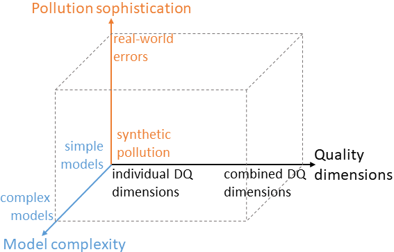
Before diving further into the details of our experimental setup, we highlight the broad scope of plausible variations of such an empirical study, showing the full perspective of any possible correlation between data quality and ML-models. As illustrated in Figure 1, there are three main aspects: (1) the model that can vary from simple models (e.g., decision trees) to complex ones (e.g., based on pre-trained embeddings); (2) the pollution/error type can range from synthetically introduced problems to more difficult-to-detect real-world errors; (3) data quality dimensions could be studied individually or by considering several dimensions at once assuming they are not independent. Together, these dimensions span an enormous experimental space. To gain the necessary basic understanding, we limit our experiments to simple models, synthetic pollution, and individual data quality dimensions. We plan to expand our study to cover the wider variations in future work.
Regarding data quality, we account for two aspects. First, data plays a different role at different stages of the ML-pipeline: Some systems use pre-trained models and thus the only available data is the “serving” or “testing” data; in many other cases, data scientists also need “training” data to build the models from scratch. Second, training and testing data can be generated or collected by the same process from the same data source, so that they have similar quality. In a more realistic case, training and testing data have different quality, especially when using pre-trained models and different sources or collection processes. To that end, we consider in this study three scenarios: Training and testing data have the same quality (Scenario 3); the training data have high quality (in terms of the studied quality dimensions) and lower quality testing data (Scenario 2); and finally, the testing data have a high quality and the data used to build the models are of a lower quality (Scenario 1).
To vary data quality in each of these scenarios, we apply the notion of data pollution or corruption to create degraded quality versions of the dataset at hand. For each of the six quality dimensions, we designed a parameterized data polluter to introduce corresponding data errors. While we used real-world data, for several of the datasets we had to manually create a clean version as a baseline to initiate the pollution process. In these cases, we report the performance of ML-models for both the “original” and the “baseline” datasets.
Research in the machine learning community has studied the effects of label noise and missing values, and the data management community has studied the effects of data cleaning on classification, as we discuss in Section 2. Nevertheless, this paper is the first systematic study of the effects of data quality dimensions not only for classification, but also for clustering and regression tasks. We studied this effect also for low-quality training data and not only for test data. Our work on real-world datasets with numerous experiments is a first step not only towards linking ML-model performance to the underlying data quality, but also to understand and explain their connection.
Contributions. We present a comprehensive experimental study to understand the relation between data quality and ML-model performance under the umbrella of data-centric AI, providing:
-
•
A systematic empirical study that investigates the relation between six data quality dimensions and the performance of fifteen ML algorithms.
-
•
A simulation of real life scenarios concerning data in ML-pipelines. We perform a targeted analysis for cases where serving data, training data, or both are of low quality.
-
•
Practical insights and learned lessons for data scientists. In addition, we raise several questions and point out possible directions for further research.
-
•
Polluters, ML-pipelines and all datasets as research artifacts that can be extended easily with further quality dimensions, models, or datasets.
Outline. Next, we discuss related work in Section 2. Then, we formally define the six data quality dimensions together with a systematic pollution method for each in Section 3. In Section 4, we briefly introduce the fifteen algorithms for the three AI tasks of classification, regression, and clustering. We describe our experimental setup in Section 5. The results of the empirical evaluation, the core contribution of this paper, are discussed in Section 6. Finally, we summarize our findings in Section 7.
2 Related Work
First, we report on the state of the art in data validation for ML. Then, we discuss related work that studies the influence of data quality on ML-models, namely by conducting an empirical evaluation, cleaning the data or by focusing on a specific error type like label noise.
Data validation.
Several approaches have emerged to validate ML pipelines as well as the data fed to them, which includes training and serving data (data used in production). These approaches use the concept of unit tests to help engineers diagnose model-quality issues originating from data errors. For instance, the validation system implemented by breck2019data (9) and the similar system by SchelterRB20 (62) focus on validating serving data given a classification pipeline as a black box.
Generally, validation systems check, on the one hand, for traditional data quality dimensions, such as consistency and completeness, and on the other hand for ML-dependent dimensions, such as model robustness and privacy biessmann2021automated (6). To help data scientists with the validation task, SchelterRB21 (61) introduced the experimental library JENGA. It enables testing ML-model’s robustness under data errors in serving data. The authors use the concept of polluters or data corruptions as in our work. However, they do not provide an extensive experimental study and their focus is on describing the framework.
Task-dependent data quality.
9458690 (23) argue that data quality assessment should not be performed in isolation from the task at hand. Our results confirm this for ML-models, as the same “low” quality data has a different effect when used to train different models. Their paper proposes a theoretical framework with a setup similar to our experiments, which evaluates the performance of a task given polluted datasets by various kinds of generated systematic noise. The proposed framework then computes the variation effect factor or the sensitivity factor from the observed results of the task. Unlike our work, however, the authors focused only on polluted training and testing data (Scenario 3 in our paper) and the experiments were conducted on a single dataset to evaluate only three models (one per ML-task) namely, Random Forest, k-means, and Linear Least Square. The authors made observations that agree with our findings, especially the fact that missing values (completnesses) are a problem for all ML-tasks.
Data cleaning.
LiRBZCZ21 (42) investigated the impact of cleaning training data, i.e., improving its quality, on the performance of classification algorithms. They obtained a clean version of the training data instead of systematically polluting it, as we did in this work. This effort yielded the CleanML benchmark. Furthermore, in their work, the robustness of the data cleaning method had an additional influence on how the classification performance changed with a training data of a higher quality. They focused on five error types: missing values, outliers, duplicates, in-consistencies, and mislabels. These error types are among the most popular error types, and thus some of them correspond to the data quality dimensions in our study. The authors observed that cleaning inconsistencies and duplicates is more likely to have low impact, while removing missing values and fix mislabeled data is more likely to improve the classifier prediction. These observations align with our findings.
The CleanML benchmark datasets have been recently used, among others, by NeutatzCAYA22 (49). The authors evaluate the ability of AutoML systems, such as AutoSklearn FeurerKESBH15 (22), to produce a binary classification pipeline that can overcome the effect of the following types of errors in training data: duplicates, inconsistencies, outliers, missing values, and mislabels. The authors concluded that AutoML can handle duplicates, inconsistencies, and outliers but not missing values. The paper also points out that most current benchmark datasets contain only few real-world errors with insignificant impact on the ML-performance even without any cleaning. For this reason and as mentioned in Section 1, our work uses synthetic errors to better characterize the correlation between ML-models performance and data quality.
Clearly, our study aligns with data cleaning efforts but with a different goal. Data cleaning systems mainly focus on cleaning the data, but our observations give data experts the understanding of the effects of data quality issues. They can then use this knowledge to determine the robustness of their insights and decide which specific problems should to be tended to and when. For an overview of the progress in cleaning for ML, we refer to NeutatzCA021 (50).
Label noise.
The problem of label noise or mislabeling is one of the main concerns of the ML-community and has attracted much interest. This problem is in essence a data quality problem. FrenayV14 (24) surveyed the literature related to classification using training data that suffers from label noise, which is equivalent to the target accuracy dimension in our work. They distinguish several sources of noise, discuss the potential ramifications, and categorize the methods into the classes label noise-robust, label noise cleansing, and label noise-tolerant. They conclude that label noise has diverse ramifications, including degrading classification accuracy, high complexity learning models, and difficulty in specifying relevant features.
abs-2103-14749 (52) focus on label noise in test data and its effect on ML-benchmark results and thus on model selection. They estimated an average of 3.3% label noise in their test datasets and found that benchmark results are sensitive even to a small increase in the percentage of mislabeled data points, i.e., a smaller capacity models could have been sufficient if the test data was correctly labeled, but the label noise led to favoring a more complex model. We report similar behavior in our discussion of the effect of target accuracy dimension on classification performance and expand the discussion to clustering and regression tasks
In summary, we present the first systematic empirical study on how both training and testing (serving) data quality affects not only classification but all the three ML tasks. We also provide a clear definition for each of the data quality dimensions and a respective method to systematically pollute the data.
3 Data quality dimensions and data pollution
We present the definition of the six selected data quality dimensions, along with our methods to systemically pollute a dataset along those dimensions. In this work, we use the ML terms feature and sample to refer to column and row, respectively. During the pollution, we assume that features’ data types and the placeholders which represent missing values in each feature are given.
3.1 Consistent Representation
A dataset is consistent in its representation if no feature has two or more unique values that are semantically equivalent. I.e., each real-world entity or concept is referred to by only one representation. For example, in a feature “city”, New York shall not be also represented as NYC or NY.
Definition 1
The degree of inconsistency of a feature , denoted as , is the ratio of the minimum number of replacement operations required to transform it into a consistent state and the number of samples in the dataset.
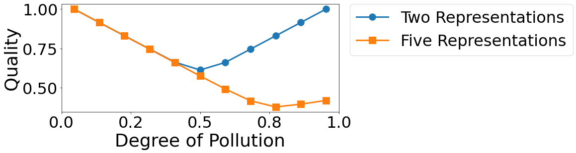
This definition applies only to categorical features, i.e., strings or integers that encode categorical values, whereas numerical features and dates are considered to be consistent and theirs . The degree of consistency of a feature cannot be derived by subtracting from 1 because it also depends on the number of representations of an original value (see Figure 2).
Definition 2
We define the degree of consistency of a dataset with features as follows.
| (1) |
Pollution.
We have two inputs: First, the percentage of samples to be polluted , defined by a value between 0 and 1, and second, for each unique value of a pollutable feature, the number of representations for that value (including itself). For each categorical feature, we choose randomly the samples to be polluted. Then, we generate new representations for each unique value of its values. The new representations of a string value are produced as new non-existing values by appending a trailing ascending number to the end of the value, whereas for integers, new integers are added after the maximum existing one. These sample’s entries at this feature are replaced by a randomly picked fresh representation of the original value.
3.2 Completeness
The problem of missing values exists in many real-world datasets. Some of these values are actually missing, e.g., missing readings due to a failure in a sensor while others are represented by a placeholder, such as “unknown” or “NaN”. For example, when medical sensors monitor temperature, blood pressure and other health information of a person and one sensor fails for a period of time, there are no values present for this sensor and time in the recorded dataset. In the case of a survey form containing optional input fields, personal attributes like the employment status could be given as “unknown”. The respective value that has a missing value could potentially be absent. When processing data automatically, for example in a data frame, the value itself usually exists, but is not informative or useful for analysis and therefore equivalent to the value being missing, decreasing the completeness of the dataset.
Definition 3
The completeness of a feature is the ratio of the number of non-missing values and , the total number of samples in this dataset. The completeness of a dataset is defined as follows.
| (2) |
A dataset with a completeness of 1 has no missing values in it. In case of a completeness of 0, the whole dataset consists only of missing values, except for the target feature. For ML, samples with a missing value for the target feature are usually removed from the dataset, as they cannot be used for training. Thus, we exclude the target feature while computing completeness. For example, consider a dataset that has 4 features and 4 samples. We exclude the target feature and only consider the remaining 3 features. This means that there are 12 values in total for computing the completeness. If 2 values are missing in the dataset, regardless of their feature and sample, the completeness of the dataset is .
Pollution.
We inject missing values “completely at random” MCAR-definition (44) according to a specified pollution percentage for each feature. If there are already missing values in the feature, we account for those values and inject only the remaining number of missing values necessary to reach . A feature-specific placeholder is used to represent all missing values injected into this feature. The placeholder value does not carry information except that the value is missing. A typical placeholder is Not a Number (NaN). Many implementations of ML algorithms cannot handle NaN values. For this reason, we choose a representation as placeholders that can be used in computations, but lie outside the usual domain of a feature and are still distinguishable from the actual non-missing values of the feature. For example, -1 for “age” feature, or the string “empty” for “genre” categorical feature in a movie table. We manually selected the used placeholders, as this task requires some domain knowledge to determine suitable values. A placeholder value representation can count as imputation SchelterRB21 (61). Most imputation methods, such as taking the mean, reconstruct some amount of information based on other observed values. As the placeholder does not contain information related to the data and has no reconstruction involved, we still consider a placeholder representation as pollution. Further, comparing different imputation methods would drift apart from the dimension completeness because it would interfere with other dimensions like accuracy. We do not make any assumptions about the underlying distribution and dependencies of missing data in our datasets. The probability of an value to have a missing value is not influenced by any other observed or unobserved value in the data. In other terms, we only consider data that is Missing Completely at Random (MCAR) MCAR-definition (44) in our experiments.
3.3 Feature Accuracy
ML-models learn correlations in datasets; thus it is desirable to have no errors in their values. For synthetic datasets, one can ensure that this is the case. However, real-world data may contain erroneous values from various sources, e.g., erroneous user input. Feature accuracy reflects to which extent feature values in a given dataset equal their respective ground truth values. The more cells deviate from their actual value and the stronger pronounced this deviation is, the lower is the feature accuracy.
Definition 4
The feature (column) accuracy measures the deviation of its values from their respective ground truth values. For a categorical feature , we define the feature accuracy as follows.
| (3) |
where denotes the number of values in the feature that are different from the ground truth and is the number of samples in the dataset. The erroneous values’ ratio is then subtracted from 1, meaning that 1 is the best possible quality and 0 is the worst possible quality. For numerical ones, we define feature accuracy as follows.
| (4) |
| (5) |
where is the average of the absolute distances between the ground truth and values in (see Equation 5) and is the mean of the ground truth values of .
In Equation 5, is defined as the index of a specific sample. Hence, denotes the ground truth and the value of the sample with index in feature . As for the categorical features, a quality of 1 indicates a clean feature. In contrast to the categorical feature quality measure, the numerical measure can fall below 0 and has no defined lower bound. However, we found that all datasets polluted reasonably also yield a numerical quality .
The feature accuracy of an entire dataset consists of two metrics: The average feature accuracy of all categorical features and the average feature accuracy of all numerical features .
This is caused by the fact that with numeric features all samples are polluted, and with categorical features only a certain percentage of the samples are polluted. Therefore, the feature accuracy of both feature types is calculated differently, which leads to both feature types having different accuracy ranges.
The feature accuracy quality measure of all categorical features is defined as the average of the feature accuracy of all categorical features as can be seen in Equation 6. Similarly, Equation 7 shows that the feature accuracy quality measure of all numeric features is defined as the average of all per-feature accuracies.The numbers of categorical and numeric features are given by and , respectively.
| (6) |
| (7) |
Pollution.
The polluter takes three arguments. The first argument is a dictionary that maps feature names to float numbers in the interval . It describes the level of pollution that should be utilized for each given feature. can also be defined as a single float number, meaning that the same level of pollution is applied to all features. The second and third polluter arguments each contain a complete list of the available categorical and numeric feature names.
The pollution is executed differently depending on the feature type. For categorical features, the level of pollution for a specific feature determines the percentage of samples to be polluted.
The samples to pollute are chosen randomly. However, the seed for this selection is fixed to (1) ensure reproducibility of the results and (2) allow for a level of pollution to be a direct extension of . The randomly selected samples are polluted by exchanging the current category with a random, but different category from feature ’ domain. Consequently, a level of pollution for a categorical feature means that the categories of all samples are updated and indicates that all categories of stay the same.
For numeric features, we add normally distributed noise to all samples of the feature : where is random samples drawn from the normal Gaussian distribution with and . The level of pollution determines the standard deviation of the normal distribution and thus denotes how wide it is spread. Again, it is ensured that the same seed is used per feature in consecutive pollution runs on the same dataset to keep the behavior consistent and comparable.
3.4 Target Accuracy
For each sample in a dataset, the target feature contains either a class/label in classification tasks or a numeric value in regression tasks. There might be some incorrect labels due to human or machine error, e.g., an angry dog labeled as a “wolf”.
Definition 5
The target accuracy of a dataset is the deviation of its target feature values from their respective ground truth values. For a categorical target, the target accuracy is the ratio of correct values in the target feature.
| (8) |
For a target with numerical values, we define the target accuracy as follows.
| (9) |
Where is the averaged sum of the absolute distances (Manhattan distance) of the ground truth and target feature values and is the mean of the ground truth values.
The definition of the target accuracy of a dataset is equivalent to the definition of the feature accuracy of its target feature (see previous section).
Nevertheless, the target feature is the most important feature because of its influence on prediction performance. Thus, it is beneficial to study its accuracy separately. By scaling with the mean, we obtain a measurement that is less dependent on the actual target domain and, thus, more comparable between different datasets. This, in theory, allows for a negative quality metric where on average every target value is more than one mean away from its ground truth. We disregard those cases and define 0 as the lowest possible quality metric in our experiments.
Pollution.
Naturally, we used the same pollution method as for feature accuracy, based on the target type. In general, this polluter takes a single argument for degree of pollution . For categorical target, this value is interpreted as the fraction of data points that should be polluted. The pollution itself replaces the current label with a randomly chosen label that differs from the current one. For numerical targets, is interpreted as the variance of normally distributed noise that is scaled by the mean of the original target value distribution and added onto the target values of the specified subset (e.g., train or test data).
3.5 Uniqueness
Redundant data does not provide additional information to the ML-model for the training process. Thus, de-duplication is a common step in ML pipelines to avoid overfitting. Furthermore, there is a plethora of existing research on how to detect duplicates and how to remove them duplicates-quality (13, 35). In this report, we evaluate how the number of duplicates present in a dataset influences the performance of ML-models. We investigate whether pre-processing datasets to remove duplicates is an essential step toward improved ML performance. According to Chen et al. there are different definitions when to consider two samples as duplicates, such as having identical primary keys or the equality in every feature of the two samples redundancy_def (12). In practice, there are also often non-exact duplicates, where some features differ slightly, for example timestamps. Introducing non-exact duplicates in the polluter would not only interfere with the redundancy dimension, but also with consistent representation (see Section 3.1). Exact duplicates are easy to detect. Yet, this step still expensive, especially for large datasets. In this regard, ideally, there are as few duplicates as possible in a dataset. Therefore, we only consider fully equal samples as duplicates.
Definition 6
The uniqueness of a dataset is the fraction of unique samples within the dataset. To make it possible to obtain a quality metric of 0, we subtract 1 from the denominator and numerator. We normalize the value as follows.
| (10) |
A dataset with the quality metric of 1 does not contain any duplicates, whereas the quality metric of 0 refers to a dataset containing only one unique record – even if the dataset contains many records overall.
Pollution.
Input datasets can contain duplicates themselves. To pollute a dataset along the uniqueness dimension, we first remove all existing exact duplicates. This allows to pollute the dataset in incremental fashion. Then, we add exact duplicates of randomly selected samples to the dataset. Actually, we increase the dataset size to avoid data loss that can affect ML-models performance. The number of the added duplicates is determined by the duplication factor : For each class with samples, we add duplicates to avoid changing the class balance (next section). Thus, the size of the polluted dataset is and its uniqueness is . The duplication factor ranges from 1, meaning no pollution is applied, to potentially infinity. It is important to decide how often each sample appears in the polluted dataset. One trivial approach would be to duplicate each by the same factor. One issue of this approach is the limited applicability to real-world scenarios. In reality, the number of duplicates per sample depends on the data domain. Manually inserted form data, for example, probably contain a normally distributed number of duplicates due to human errors, with a mean of 2. Working with sensor data, due to misconfiguration of sensors, the distribution of duplicate count could be uniform. Analyzing web index data based on web traffic, the duplicates could be distributed according to the Zipf distribution. Thus, the polluter needs to be flexible regarding the distribution of duplicate counts per sample. For each randomly selected sample from a class , we add duplicates of this sample and then continue sampling and adding duplicates to reach . We draw from a pre-defined distribution: We try uniform, normal, and Zipf distributions, in addition to adding a single duplicate of each selected sample. The duplicate counts generated by the specified distribution function define only the number of duplicates to add for the respective sample each time the sample is randomly selected for duplication. For this reason, the actual resulting distribution of duplicate cluster sizes after pollution likely differs from the specified distribution. This can happen especially with large duplication factors, but is inevitable, as otherwise classes with a low number of sampled duplicate counts could limit the number of generated elements.
3.6 Target Class Balance
Many ML approaches assume a relatively equal number of samples per target class, i.e., a balanced dataset, to achieve satisfactory performance. Clustering or classification algorithms on top of a highly imbalanced dataset may fail at identifying structures or even miss smaller classes completely. For example, the k-Means algorithm suffers from the “uniform effect”, i.e., it recognizes clusters of approximately uniform sizes even if it is not the case in the input data kumar2015subset (39).
Definition 7
Given a dataset with target classes of samples per class, respectively, and , the target class imbalance is defined as the sum of the pairwise differences between the number of samples per class:
| (11) |
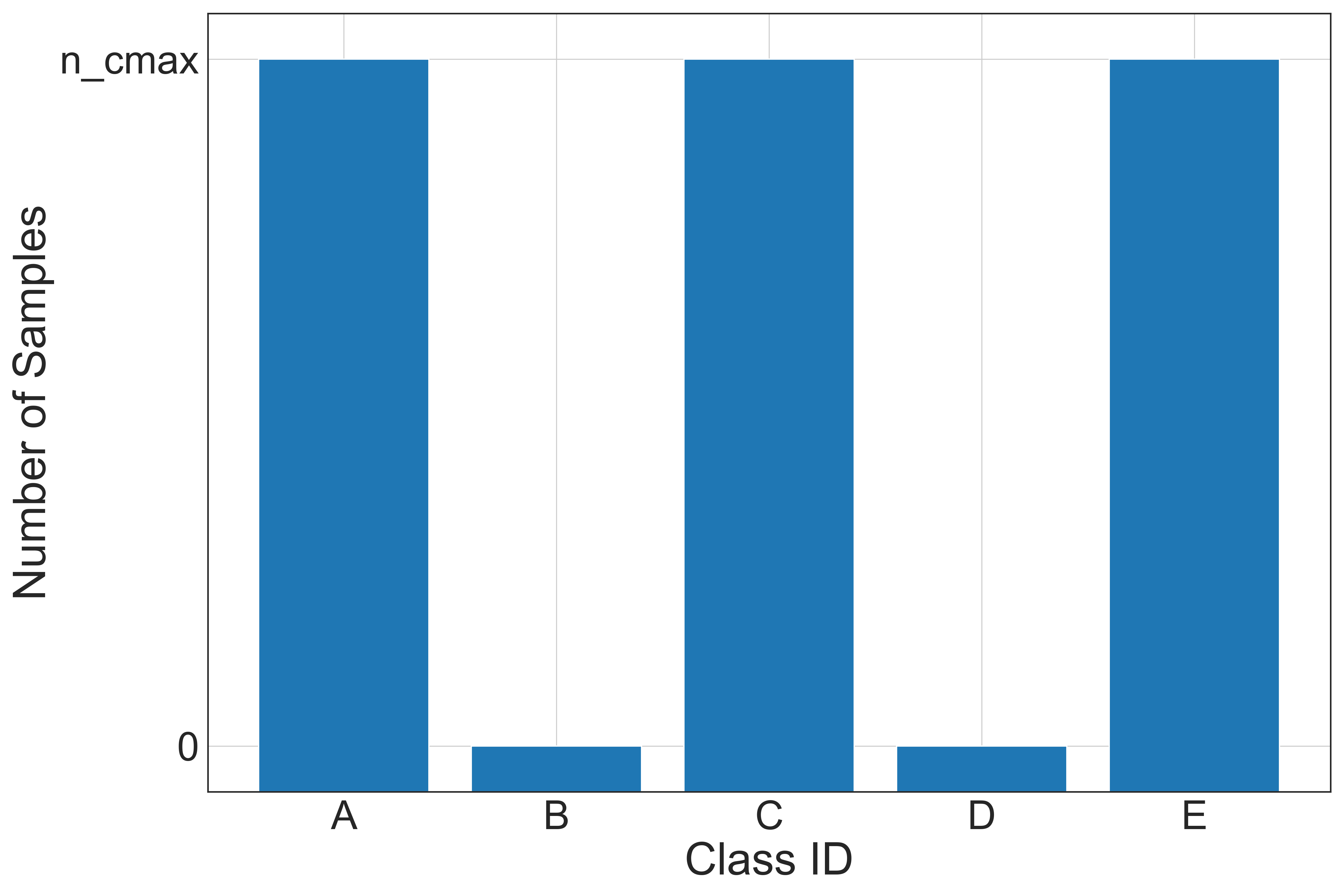
As the worst imbalance case, we assume a maximal imbalanced dataset that has classes with samples and the remaining classes have 0 samples, where is the maximum number of sample that a class can have (see Figure 3). The target class imbalance of such a dataset is . This is clearly a hypothetical case, as no class exists if it has samples; otherwise we could add infinite classes with samples to each dataset. However, this constructed the worst case allows us to define the target class balance quality measure.
Definition 8
The target class balance of a dataset is the deviation from its imbalance score, normalized by the imbalance score of the worst case.
| (12) |
If all classes in the dataset have the same number of samples, then is maximal and equals 1. Contrary, reaches its minimum () if the balance of the classes in the dataset approaches the hypothetical worst case.
Pollution.
We have two inputs for pollution: The degree of imbalance and the number of samples in the polluted version . We can choose arbitrarily as a multiplication of or calculate it from the data as the number of samples from the original dataset, needed to produce the maximum pollution level. In both cases, its validity at the maximum imbalance level and the balanced dataset is checked once more. In case of an invalid sample count, the next valid, smaller possible sample count is calculated and used while a warning is presented to the user. For calculating , we also consider that each class must have a minimum number of samples in the original dataset to be able to produce this imbalance. If this requirement cannot be satisfied, a new number of total samples in the imbalanced dataset is iteratively determined until it is possible to create the maximal imbalance. We use , which determines the severity of the class imbalance, to calculate the number of samples per class in the polluted version. It is a number in the interval and it is not directly linked to : creates a fully balanced dataset, which is to be used as a baseline for comparing all the imbalanced datasets to, as the original dataset maybe imbalanced itself; creates the most heavily imbalanced dataset. Note that the dataset produced by is not the hypothetical worst case mentioned in the definition section above. Instead, it produces a dataset where the smallest class has of the samples of the largest class and where our restriction of constant changes in sample counts between the classes still stands. While mathematically this polluted dataset with one class completely removed would be the most imbalanced, this does not suit the purpose of examining the effects of class imbalance on the ML process. Therefore, we restrict the most heavily imbalanced dataset to have a class containing the maximal number of samples and a class containing the minimal number of samples. Due to this calculation, the class balance polluter works best if the class has at least samples. This state of imbalance is reached at a degree of imbalance . However, anything above this degree is ignored by the polluter. The degree of imbalance for any polluted dataset version satisfies: .
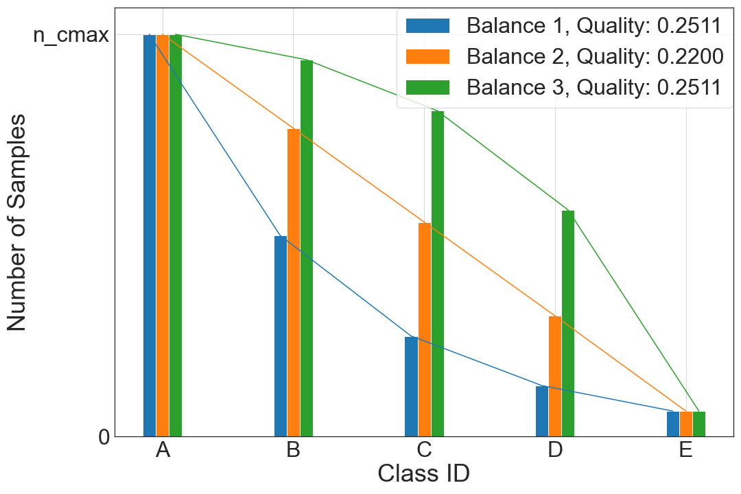
To pollute, we order the target classes based on their sizes descending and for the classes with the same size, we use the class ID in ascending order. Using the defined order, we create a class imbalance with an equal difference for each consequent pair of classes. The used samples of each class are randomly selected, i.e., in the polluted dataset, the following holds: . An example of such a distribution can be seen in Figure 4 in the depicted Balance 2. This choice has been made to both simplify the pollution process by removing all the other possible methods of creating an imbalance and make it more easily reproducible as no random component is needed to determine the per-class sample counts in the polluted dataset. Figure 4 shows the two per-class sample count distributions Balance 1 and Balance 3, which exemplify the need to limit the pollution method as they differ in per-class sample counts but still produce the same dataset quality.
To create a class imbalance, we calculate the class size of a balanced dataset with samples and classes. Then, we iteratively add/remove samples from the classes based on their order: We remove samples from all classes that are at indices and below, and add samples to all classes at indices above that, unless is odd, then the size of the class at index stays constant.
4 Machine Learning tasks
In this section, we introduce the 15 algorithms that we employed for the three tasks of classification, regression and clustering.
Classification.
We picked a variety of classification algorithms that fall into different categories. We included two linear classification models: Logistic regression (LogR) McCullaghN89 (46) and support vector machine (SVM) cortes1995support (16); a tree-based model: Decision tree (DT) Breiman1983ClassificationAR (11); a k-nearest neighbors (KNN) classifier altman1992introduction (3); and finally a neural network-based multi-layer perceptron (MLP) neural_networks_article (68).
Regression.
Regression is a supervised learning method that uses labelled data to learn the dependency between features and a continuous target variable. There is a plethora of regression algorithms. To evaluate how error-prone different categories of regression algorithms are and how more complex algorithms within one category perform, we compare five of the most widely used approaches for regression out of three categories of regression algorithms. We use two linear-regression-based algorithms: linear regression (LR) montgomery2021introduction (47) and ridge regression (RR) hoerl1970ridge (32); two tree-based algorithms: decision tree regression (DT) Breiman1983ClassificationAR (11) and random forest regression (RF) breiman2001random (10); and finally a deep-learning based algorithm: simple multi-layer perceptron (MLP) neural_networks_article (68). The most basic regression approach is linear regression. It learns a linear relationship between features added by an intercept term montgomery2021introduction (47). The second algorithm in the field of linear regression is ridge regression, which is an improved linear regression approach. It adds L2 regularization to linear regression to prevent correlated features influencing the error drastically and to prevent extremely large values in the weights hoerl1970ridge (32). The first tree-based algorithm we use is decision tree regression. It introduces axis-parallel split criteria for various features, and thus creates a hierarchical split depending on the meet conditions Breiman1983ClassificationAR (11). According to last2002improving (40), decision tree algorithms are unstable. This means minor changes in data can lead to larger changes in tree layout or changes in predictions. An improved version of decision tree regression is random forest regression. It uses ensemble learning with multiple decision trees to predict the target variable. As a result, it is less error-prone and more stable breiman2001random (10). Deep learning is a machine learning approach that is more and more commonly used among all fields of machine learning. Thus, it can also be used for regression. We use a simple multi layer perceptron in this category of algorithms neural_networks_article (68).
Clustering.
Clustering algorithms aim to find groups of samples with similar features in a given dataset. Since clustering is an unsupervised approach, our clustering models are not trained but directly receive all data as test data for the prediction of the target label. Depending on dataset properties, such as dimensionality, distribution or data types, current research recommends different clustering algorithms. These can be grouped into different categories or algorithm families. We decided to use one algorithm from each of the five most commonly used categories of clustering algorithms rokach2005clustering (58): The Gaussian Mixture Clustering algorithm reynolds2009gaussian (57) from the distribution-based family, the k-Means sinaga2020unsupervised (65) and the k-Proto-types ji2013improved (36) algorithms from the centroid-based family, the Agglomerative Clustering algorithm day1984efficient (17) from the hierarchical family, the Ordering Points to Identify Cluster Structure (OPTICS) algorithm ankerst1999optics (4) from the density-based family and a Deep Autoencoder neural network from deep learning-based family song2013auto (67).
The Gaussian Mixture Clustering algorithm is a distribution-based approach and assumes the input data to be drawn from a mixture of Gaussian distributions reynolds2009gaussian (57). It aims to fit a Gaussian distribution to each cluster whereby a sample can be assigned to several clusters, each with a certain percentage. Thus, the mean and the standard deviation describe the shape of the clusters which allows for any kind of elliptical shape. The algorithm starts with random distribution parameters per cluster. In each iteration, the probability of each sample belonging to a particular cluster is calculated. The probability is higher the closer the sample is to the distribution’s center. Afterwards, the parameters for the Gaussian distributions are updated according to the probabilities. A new iteration is performed until the distributions no longer change significantly.
For the centroid-based category, we either apply the k-Means sinaga2020unsupervised (65) algorithm for datasets with predominantly numerical features or the k-Proto-types ji2013improved (36) algorithm for datasets with a large number of categorical features. The former is initialized with a random center point for each of the given target classes. Thereafter, each sample is assigned to its closest center point and all center point vectors are updated with the mean of all sample vectors currently assigned to the respective center point. This procedure is repeated until the center points do not change their positions much. The k-Prototypes algorithm represents a combination of k-Means and k-Modes algorithms. The latter can only deal with categorical features, utilizing the number of total mismatches (dissimilarities) between the samples instead of the actual distance like k-Means does. Thus, for categorical features, k-Prototypes assigns each sample to the cluster with which it has the fewest dissimilarities and for numerical features, it applies k-Means.
The hierarchical family of clustering algorithms is represented by the Agglomerative Clustering algorithm day1984efficient (17). It expresses the hierarchy of the clusters as a tree, i.e., the leaves are clusters with a single sample each and the root is one big cluster containing all samples. Starting with one cluster per sample, the algorithm merges two clusters into one per iteration based on a given distance measure. Therefore, in each step, each cluster is combined with the cluster closest to it until the root of the tree is reached. Depending on how many clusters should be build, this procedure can be stopped earlier.
We selected the Ordering Points to Identify Cluster Structure (OPTICS) algorithm for the density-based clustering category ankerst1999optics (4). On a high level the OPTICS algorithm works similar to the Density-Based Spatial Clustering of Applications with Noise (DBSCAN) algorithm, identifying areas of high density within the data and extending clusters outwards from these cores ester1996density (20). In contrast to the DBSCAN algorithm, OPTICS uses these identified core regions to calculate a reachability distance for each data point to the closest core. Using this reachability distance, and a calculated point ordering, a reachability plot is generated. From this, clusters can be identified by searching for extreme changes in the reachability distance between neighboring points at which point clusters are then separated and, if applicable, outliers identified. This approach is more versatile than the approach DBSCAN takes, justifying our selection of this clustering algorithm for our use-case where we do not want to run hyperparameter optimization. The sklearn implementation of the OPTICS algorithm we use in our work differs slightly from the approach originally described by ankerst1999optics (4) in the way in which cores are initially identified sklearn_optics (18).
To represent the deep learning-based clustering methods, we chose to implement a Deep Autoencoder neural network to aid with the clustering process. The Autoencoder is used as a data preprocessing step in this approach, transforming the input data which may lie in a high-dimensional space or generally a space not conducive to clustering into the lower-dimensional code space, which may be more suitable for the clustering task. The Autoencoder itself is trained to learn how to map the input data into the code space and then decode it again while trying to minimize the reconstruction error, i.e., maximize the similarity of the input data and reconstructed data song2013auto (67). After the Autoencoder was trained, the encoder portion of the network is used to encode the dataset to be clustered and a classical clustering algorithm is applied to the encoded information lu2021dac (45). After experimentation, we selected the Gaussian Mixture algorithm over the k-Means clustering algorithm for this task.
Our Autoencoder is a very basic neural network and built dynamically, depending on the number of features in the input dataset. Each of its encoder layers is a linear layer halving the number of features from its input to its output. The ReLU function is applied after each linear layer on its outputs. The encoder layers halve the number of features until only two dimensions remain, at which point we have reached the code space. The decoder has the same but inverted architecture of the encoder portion of the network.
5 Experimental setup
This chapter gives an overview of our implementation and introduces our datasets together with the parameterization and performance measures of the analyzed ML-models.
5.1 Hardware
We ran our experiments on a DELTA D12z-M2-ZR machine. The server has AMD EPYC 7702P Xeon (2.00GHz-3.35GHz, 64-Core) processor, 512 GB DDR4-3200 DIMM RAM and runs Ubuntu 20.04 LTS Server Edition. The server has two NVIDIA Quadro RTX GPUs (5000/16GB, A6000/48GB).
5.2 Implementation
The implementation of the polluters and ML pipelines are written in Python (version 3.9.7) using the scikit-learn sklearn_main (53) (version 1.0.1) and PyTorch pytorch_main (21) (version 1.10.2) supporting NVIDIA CUDA 10.2 cuda_main (15) libraries.
We evaluate the performance of the ML-models in three scenarios: Scenario 1 – polluted training set; Scenario 2 – polluted test set; and Scenario 3 – polluted training and test sets. Note that those scenarios are only considered for classification and regression, as clustering does not have a separate training and test set. To create the scenarios, we randomly split the data with a stratified 80:20 split into training and test set.
We then pollute the training and test sets separately. We varied the ratio of pollution between 0 and 1 in increments of . For consistent representation, we tested and where means adding one new representation per in the polluted dataset. For uniqueness experiments, we varied from 1 to 5 in steps to lead to linear quality decrease by per step, i.e., etc. We make the cut at a of 5, because for lower quality increases faster than linearly, e.g., would have to be 10 for a quality of 0.1, which would make the experiments much slower. Regarding duplicate count distribution functions, all samples get a duplicate count of 1 and we used a normal distribution with mean 1 and standard deviation 5.
Before applying any ML-model, we one-hot encode the categorical features. Then, we measure the performance of the respective ML-models, given the specific scenario for the specific dataset polluted with the specific polluter configuration. We run each polluter configuration five times with a different random seed, i.e., we obtain five results per ML-model in that setting, which we then aggregate by averaging.
For regression, we discretized the data with manually specified bin-step sizes before the stratified split. We use the discretized version also for the class balance and uniqueness polluters, as they require the target feature to consist of discrete classes. For all other polluters, we use the original continuous representation. The target feature distribution in our regression datasets is mostly close to a normal distribution.
When applying the class balance polluter, this would lead to a heavily decreased dataset size of much less than after balancing. That is why, when using the class balance polluter, we discard the discretized classes with very few samples, which would result in a balanced dataset with such a small size. To allow consistent comparisons with the original dataset, i.e., have the same classes contained in the data, we discard those classes with few samples from the original dataset too for the experiments with the class balance polluter.
5.3 Models Parameters
All parameters not explicitly stated are kept at their default values in scikit-learn.
Classification.
For LogR, we increase max_iter to 2 000 for better convergence. For a multi-class dataset, we fit a binary problem for each label. The maximum number of iterations for the multi-layer perceptron is 1 000. For SVM, we use a linear kernel and scale the input data with the sklearn StandardScaler, as the time to converge would otherwise make it infeasible given the large number of experiments we run.
Regression.
For LR and RF, we set n_jobs to to use all available processors. We seed all algorithms that provide a random_state parameter with 12345, which are all algorithms except LR. For MLP, we increase the max_iter parameter that defines the maximum number of epochs to 3 000 so that MLP is able to converge when trained on the original datasets.
Clustering.
The actual number of clusters is passed to the k-Means / k-Prototypes, Gaussian Mixture and Agglomerative algorithms. If categorical features exist, the Agglomerative algorithm uses the Gower’s distance measure gower1971general (26). We set the affinity parameter to “precomputed” (a pre-calculated distance matrix is to be employed) and the linkage parameter to “average”, which defines the distance between two clusters as the average distance between all samples in the first and all samples in the second cluster. For OPTICS, we only defined the minimum cluster size parameter min_cluster_size, which specifies how many samples need to be in a cluster for it to be classified as such, as 100. We chose this number based on a combination of experiments and knowledge about our data. We are certain that in our original datasets, each cluster contains substantially more samples than 100. Our Autoencoder is trained for 200 epochs and optimized using the Adam optimizer kingma2014adam (38) with a learning rate of 0.003 and mean squared error loss. The dataset is split into train and 20 test data and loaded in batches of 128 shuffled samples. For all models that need a random seed, we used 42 as a seed.
5.4 Datasets
To investigate the correlation between the studied data quality dimensions and the chosen ML algorithms, we use the nine datasets, shown in Table 5.4. We chose them from a variety of domains, sample sizes and characteristics. Our choice was also influenced by the ML-task that the dataset is used for.
| Name | # | ||||
| # | |||||
| # | |||||
| # | |||||
| # | |||||
| Classes | |||||
| Classification | |||||
| Credit | 1,000 | 20 | 13 | 7 | 2 |
| Contraceptive | 1,473 | 9 | 7 | 2 | 3 |
| Telco-Churn | 7,032 | 19 | 16 | 3 | 2 |
| Regression | |||||
| Houses | 1,460 | 79 | 46 | 33 | - |
| IMDB | 5,993 | 12 | 8 | 4 | - |
| Cars | 15,157 | 8 | 3 | 5 | - |
| Clustering | |||||
| Bank | 7,500 | 3 | 2 | 1 | 6 |
| Covertype | 7,504 | 54 | 44 | 10 | 7 |
| Letter | 7,514 | 16 | 0 | 16 | 26 |
Classification.
IBM’s Telco Customer Churn dataset represents 7043 customers from a fictional telecommunications company telco_dataset (34). It contains personal information about customers (e.g., gender and seniority) and their contracts (e.g., type of contract and monthly charges). The target variable Churn describes whether the customer cancelled their contract within the last month. We dropped the customerID sample because of its lack of information content for the classification task. The original German Credit dataset was donated to the UCI Machine Learning Repository in 1994 by Prof. Hans Hofmann credit_dataset (33). Then a corrected version was introduced by Ulricke Grömping who identified inconsistencies in the coding table and corrected them credit_dataset_corrected (28) (we use the corrected version). The German Credit dataset contains a stratified sample of 1 000 credits between the years 1973 and 1975 from a southern German bank credit_dataset_corrected (28). It contains the personal data about people who applied for a credit (e.g., marital status or age) and about the credit itself (e.g., purpose or duration). The target variable tells whether a customer complied with the conditions of the contract or not. The Contraceptive Method Choice dataset was part of the 1987 National Indonesia Contraceptive Prevalence Survey, asking non-pregnant married women about their contraceptive methods contraceptive_dataset (43). The dataset consists of 1 473 samples containing personal information about the wife’s and husband’s education, age, the number of children and much more. The classification task is to determine the contraceptive method choice out of No-use, Long-term and Short-term with the target variable Contraceptive method used.
Regression.
The Houses dataset was created as a modern replacement of the widely used but outdated Boston Housing dataset boston-house-prices (31). Located in Ames, Iowa, it contains features of houses in the city to determine their sales price ames-house-prices (14). We use the dataset in the form it was presented in a Kaggle challenge houses-dataset (37). There, only the training set includes the sale prices, which is why we take the training set with 1 460 samples from the challenge. We removed the Id feature because its only purpose is to identify houses uniquely. This results in 79 features and the target feature. There are missing values (NaN) in five features, which we replaced by computationally usable placeholders. One numerical feature, the year a garage was built, contains information related to the categorical feature garage type and has missing values for observations where the garage type indicates that there is no garage anyway. In those cases, we set 0 as a placeholder for the garage year to represent the meaning in context with the garage type to distinguish them from the MCAR values that the polluter injects in our experiments. For the remaining four of the features with missing values, their occurrence is independent of other features. We treat them as MCAR values and represent them as placeholders outside the feature domains. The IMDB dataset contains features and ratings for films and series that were retrieved from the IMDB website imdb-dataset (55). We removed all samples where the rating is missing because it is the target attribute. For the remaining 5 993 samples, we remove the name feature, as it only identifies the films and series. There are 12 features remaining apart from the target feature, where two inherently numeric features contains missing values as text placeholders. For the first feature, duration, where the missing values are unrelated to other features, we set a numeric placeholder outside the domain to be able to process the feature values as numbers instead of categories. For the second feature, episodes, there are only missing values for film elements. We do not count those as MCAR values because they are related to the fact that the element is a film and therefore contain information, which is why we set the placeholder to 0 here. The Cars dataset collects listings for used cars of different manufacturers cars-dataset (1). It contains technical attributes of the cars, as well as model, year, and tax. The sales price is the feature that shall be predicted. The data is stored in files grouped by manufacturer. We use only the data of VW.
Clustering.
The Letter dataset contains 20 000 samples of different statistical measures of character images letter-dataset (66, 19). Each sample describes one of the 26 capital letters in the English alphabet and was generated by randomly distorting pictures of the letters in 20 different fonts.The measured statistics were scaled, bounding the feature values to integers in the range . As this dataset does not contain categorical features, it is the only dataset that the consistent representation polluter cannot be applied to. This is a deliberate decision, as the majority of existing clustering datasets do not contain categorical features, and we would like to examine the other data quality dimensions on a clustering-typical dataset. The Bank dataset was created through marketing campaigns of a banking institution conducted via phone calls. It contains different characteristics of a person and has a binary target stating whether a term deposit is subscribed bank-dataset (60, 48). For clustering, however, having only two clusters is not the norm and, hence, not a representative use-case for our experiments. We use a subset of this dataset, taking the education level as the target and keeping only three features related to it to have more than two clusters. We removed all classes with less than 2 000 samples to avoid significant data loss when applying the target class balance polluter. The Covertype dataset was created by the Colorado State University and consists of descriptive information about forested areas and thereby helps natural resource managers in their decision-making processes covertype-dataset (7, 8). Each sample contains cartographic measures for an observation of a 30×30 m cell. Numerical features like the slope or elevation and categorical features like the wilderness area or soil type can be used to derive the cover type, i.e., the dominant forest type in the study area. Exemplary target classes are “Spuce/Fir” and ”Krummholz”. All datasets used for the evaluation of clustering approaches were sampled as the last step of their preprocessing to reduce their size. The sampling was conducted in the same manner for all datasets: 7 500 samples were targeted for each of the datasets, however, we wanted to sample equally many data points for each class, creating a balanced dataset in the process. We slightly varied the number of samples selected per dataset to be a multiple of the dataset’s class count larger than 7 500. Instead of sampling once, we decided to also use the same five random seeds used for any random operations in the polluters to create a total of five preprocessed datasets per raw dataset. This choice was made to account for the potential impact the sampling may have on the data if done using only one seed. However, since this increased our number of datasets from 3 to 15, we decided to limit ourselves to using only the random seed a dataset was sampled with to initialize any pollution applied to it, thus, reducing the number of polluters applied to each of our 15 datasets by a factor of 5 and still ending up with the same number of combinations of preprocessed dataset and pollution.
5.5 Models Performance
Classification.
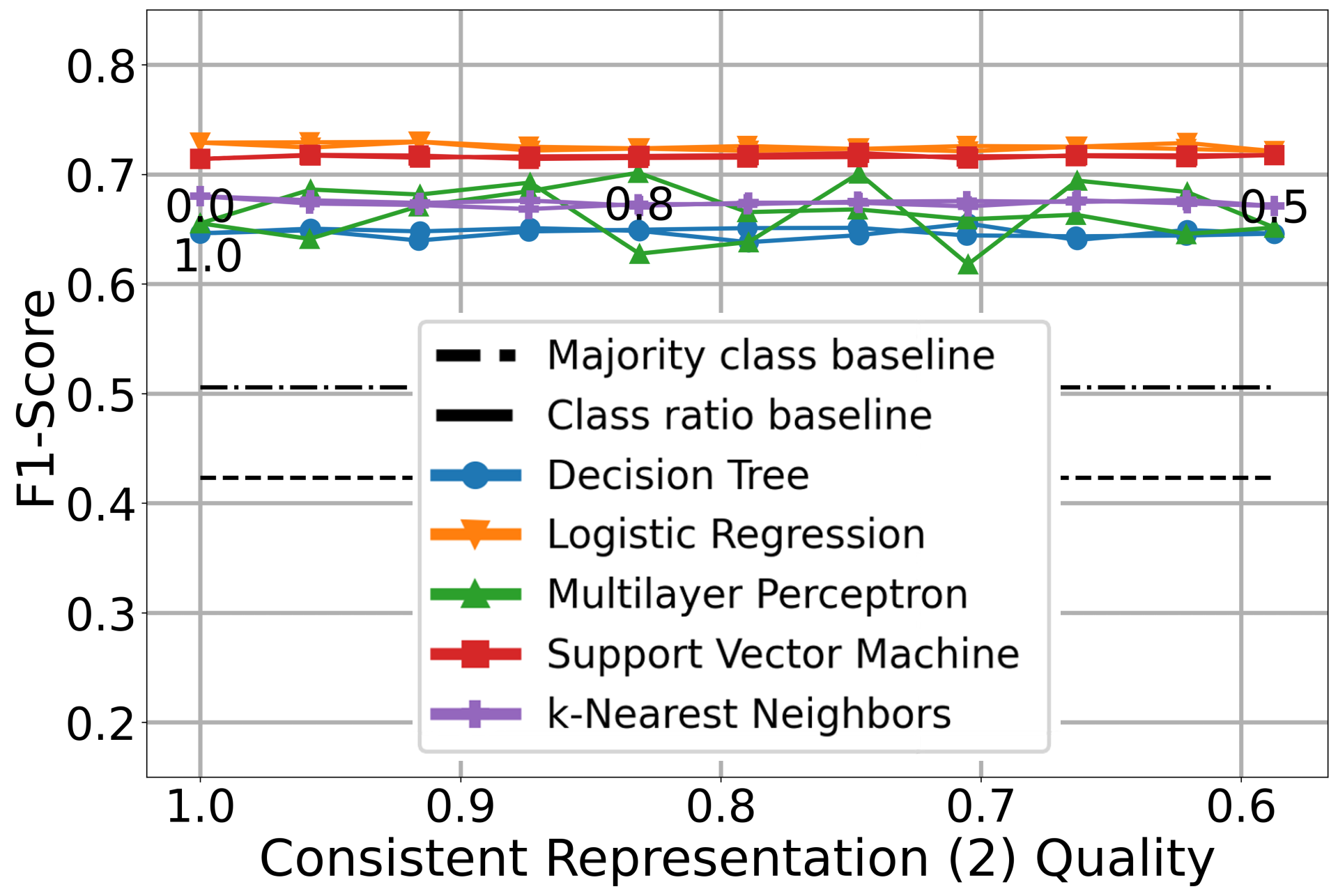
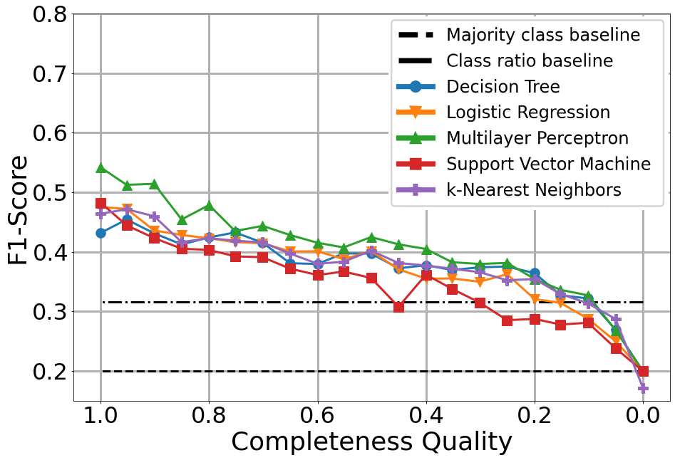
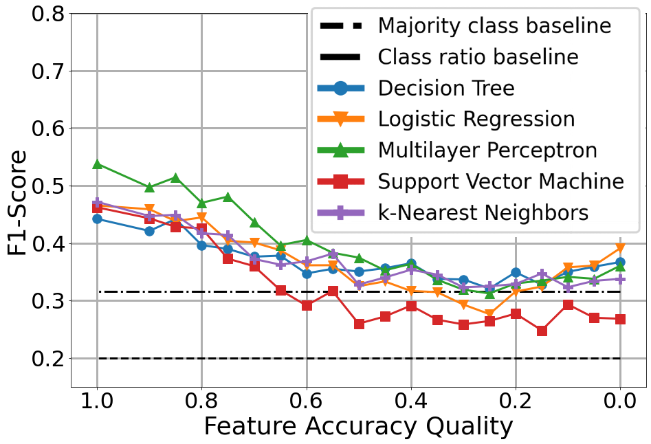
Accuracy, the number of correct predictions over the number of total predictions, is the most common performance metric in classification tasks, but it can be misleading in imbalanced datasets. For example, a majority class prediction baseline yields a 90 % accuracy on data that is naturally distributed among two classes with a ratio of 9:1. Therefore, we use -score as it better accounts for class imbalance, which does exist in the used datasets. For instance. the Telco and Credit datasets are unbalanced in their target classes, with a 70/30 split or worse. Usually, the -score is measured for a single target class, but as we do not make assumptions about the importance of the target class, we report the average of the -scores over all target classes.
Regression.
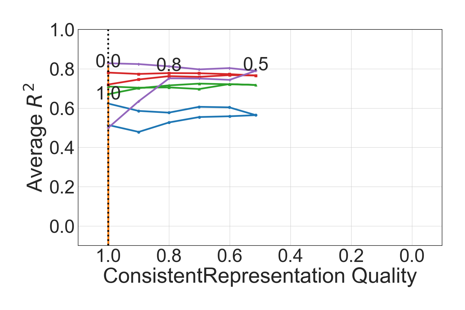
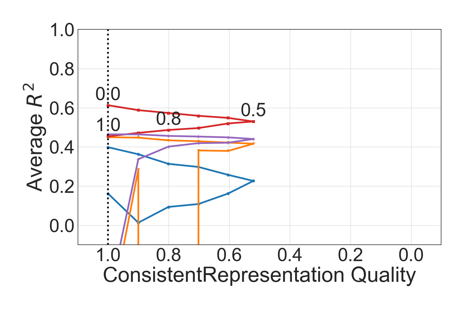
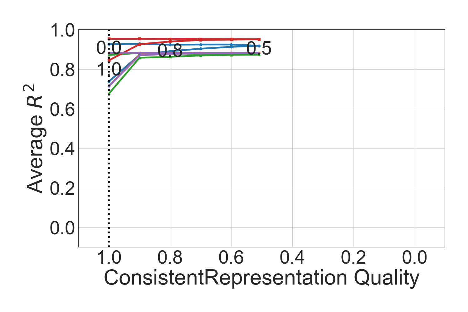
Mean Squared Error is the commonly used metric to evaluate regression algorithms. However, it is highly dependent on the data domain, e.g., it is expected to be much larger for house prices than for movie ratings. As this makes comparisons of algorithm performance across datasets difficult, we use the Coefficient of Determination , which measures the fraction of variance in the data that is explained by the regression model lewis2015applied (41). An of means that the model explains all variance, while a model that achieves an of is as good as one that always predicts the mean of the target feature regardless of the input. If is negative, the model’s predictions are even less accurate than always predicting the mean.
Clustering.
The Mutual Information (MI) score describes how much information is shared between two clusters. This metric only recognizes if the same samples are grouped with the same other samples, regardless of the actual target labels. We use an adapted version of MI called the Adjusted Mutual Information (AMI) NguyenEB09 (51). This version corrects the MI score for random choice and normalizes its value to a range between 0 and 1 which is necessary as the MI score tends to increase as the number of clusters increases, regardless of the quality of the clustering produced vinh2010information (71).
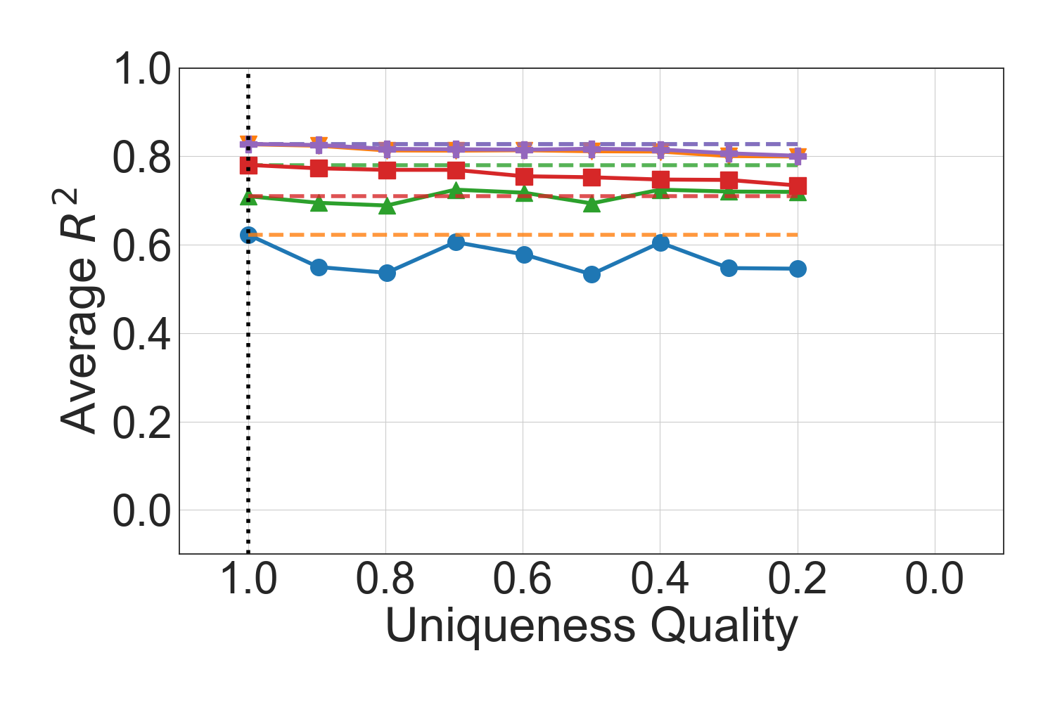
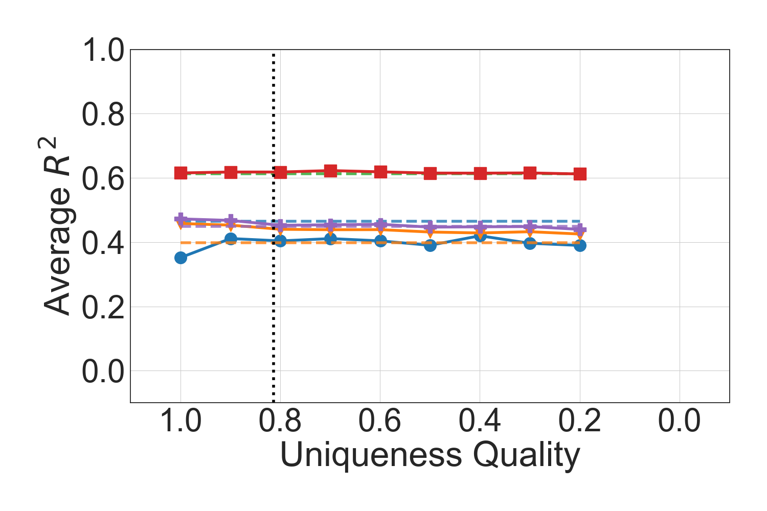
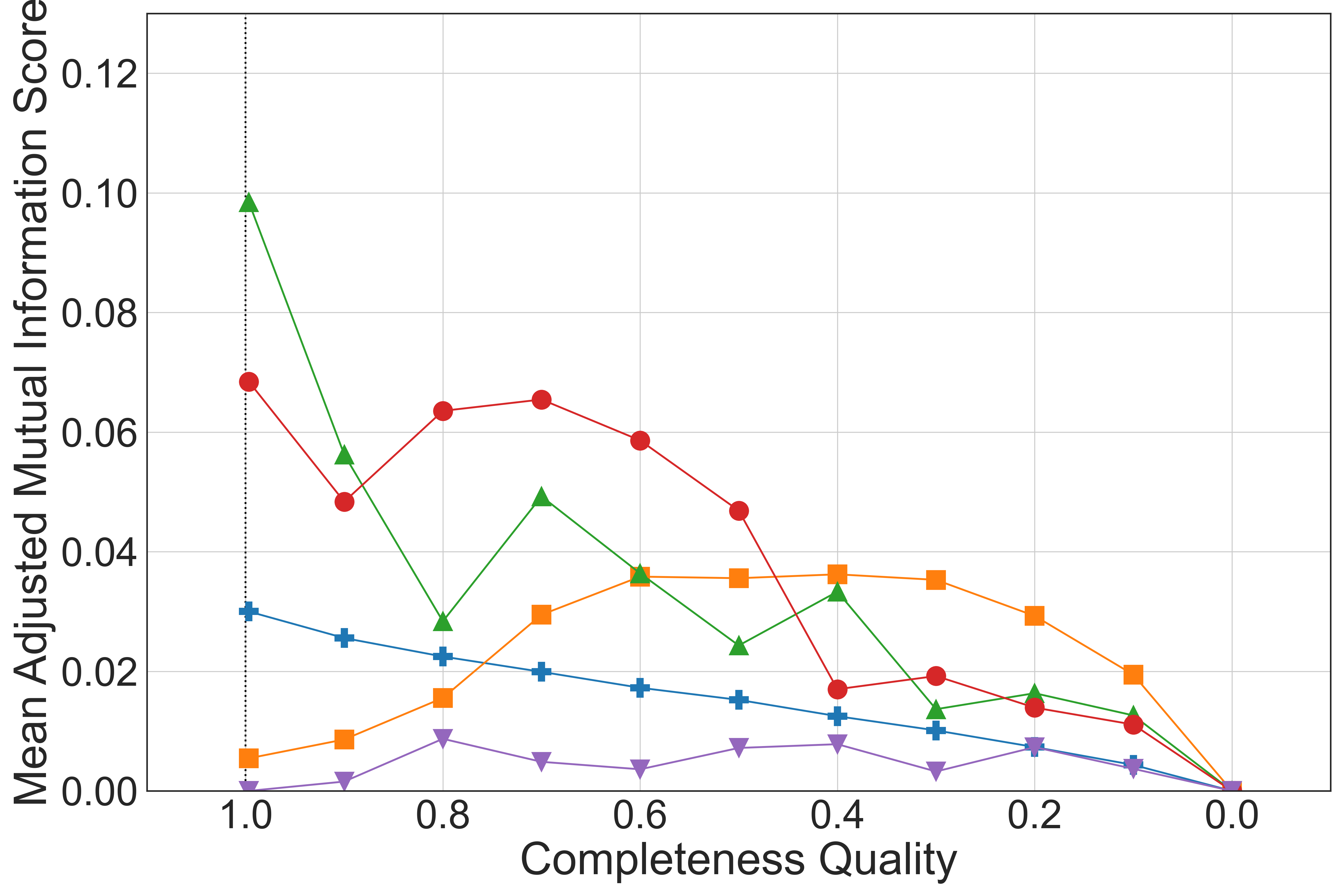
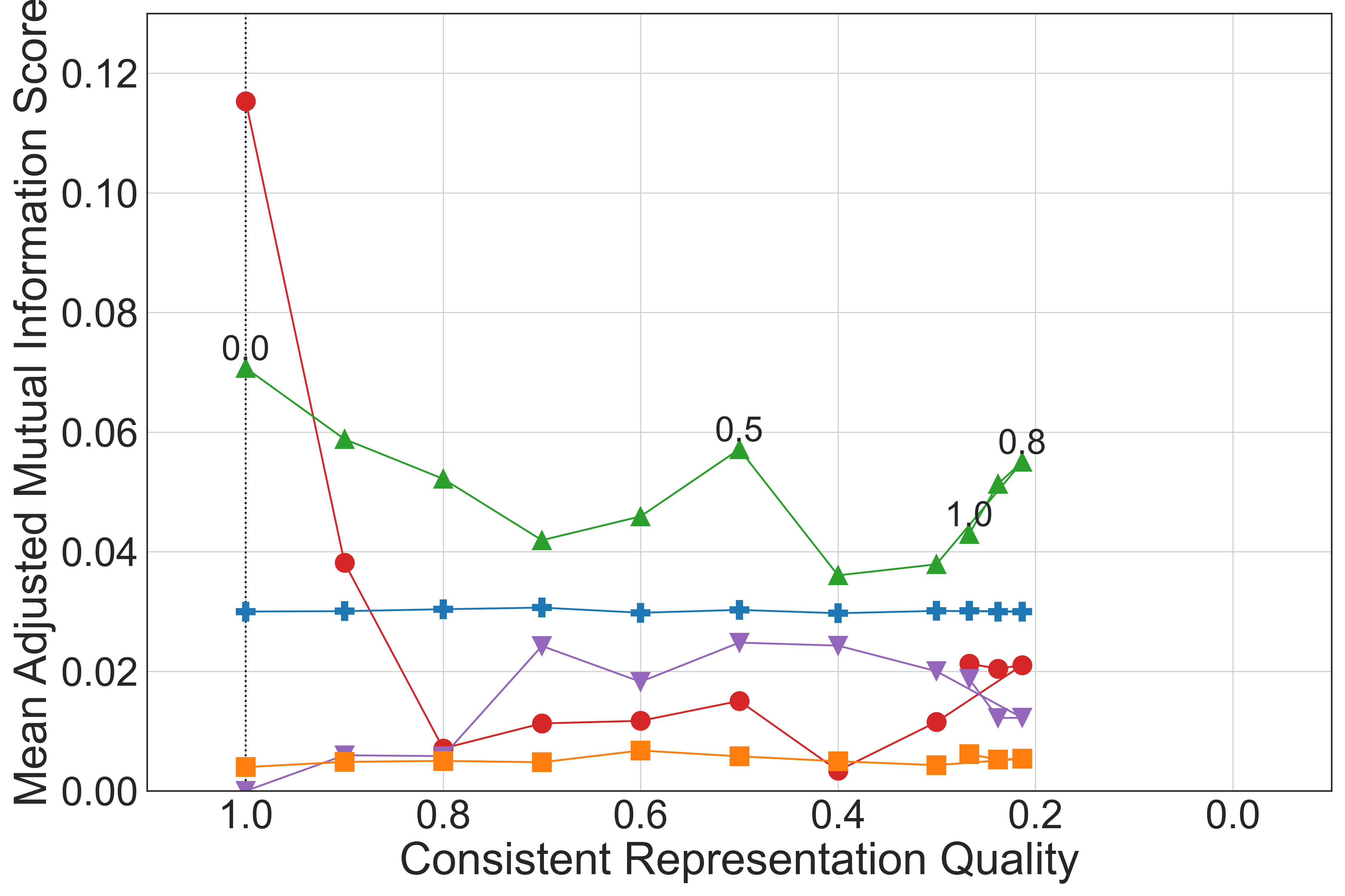
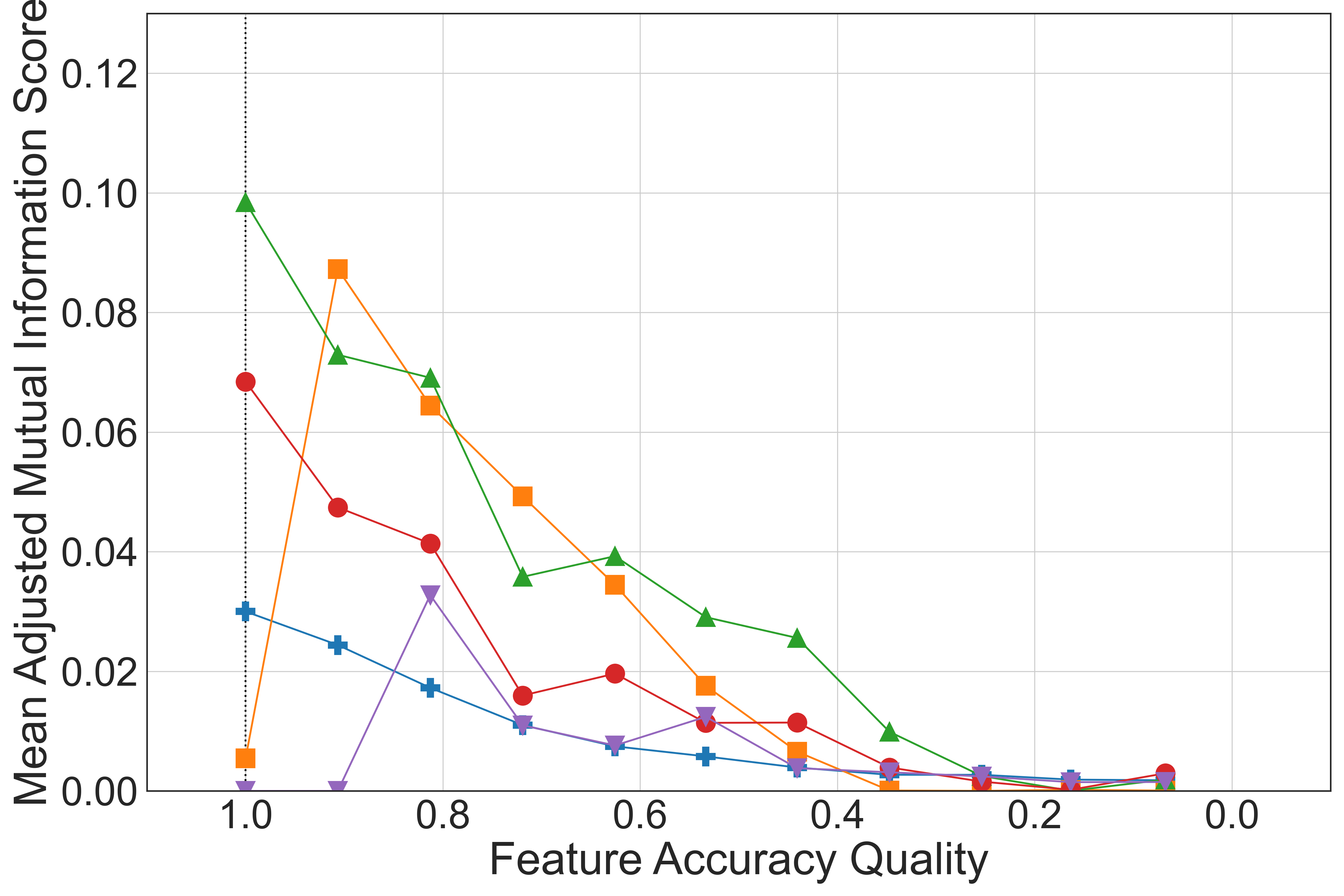
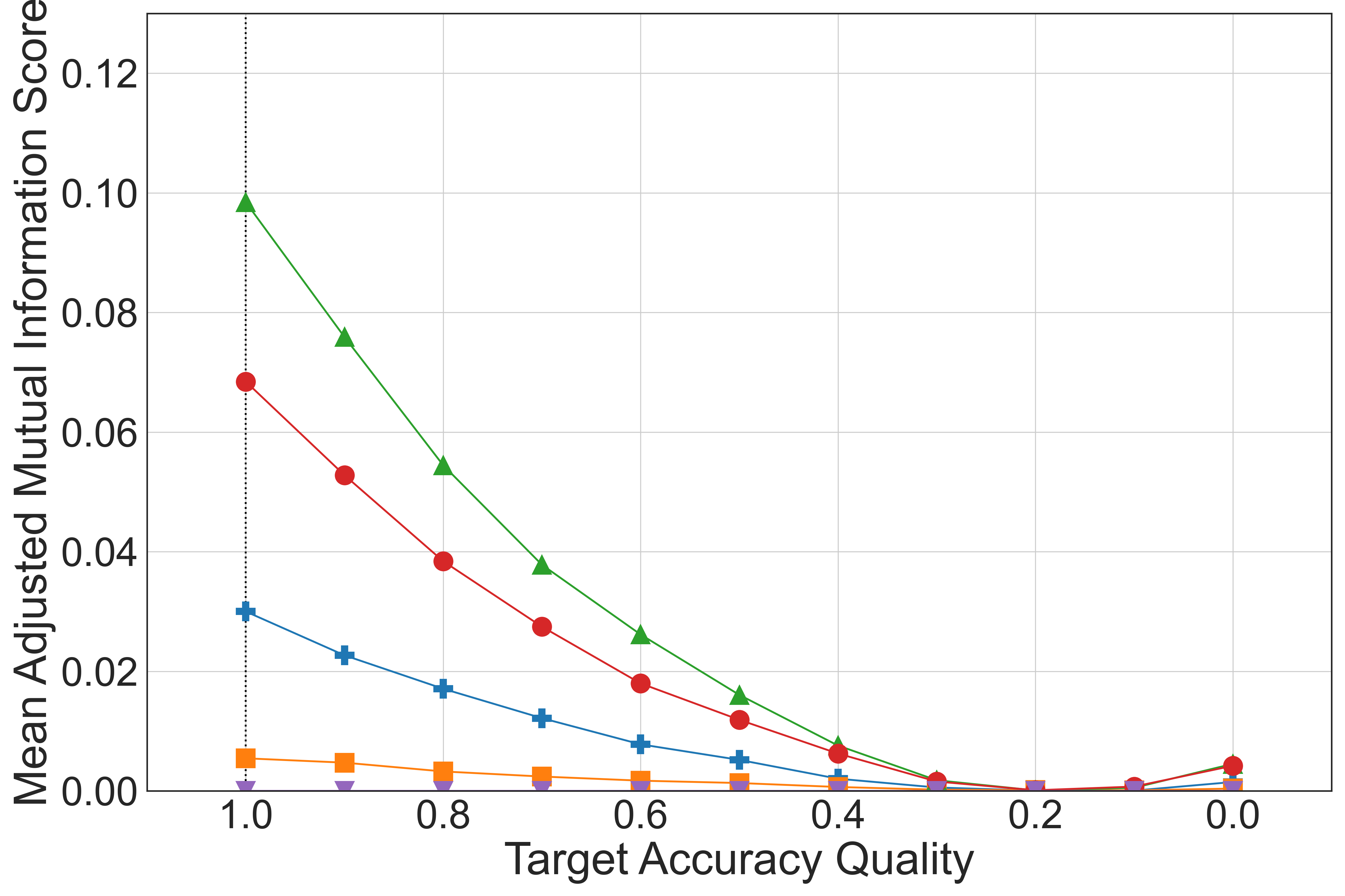
6 Results
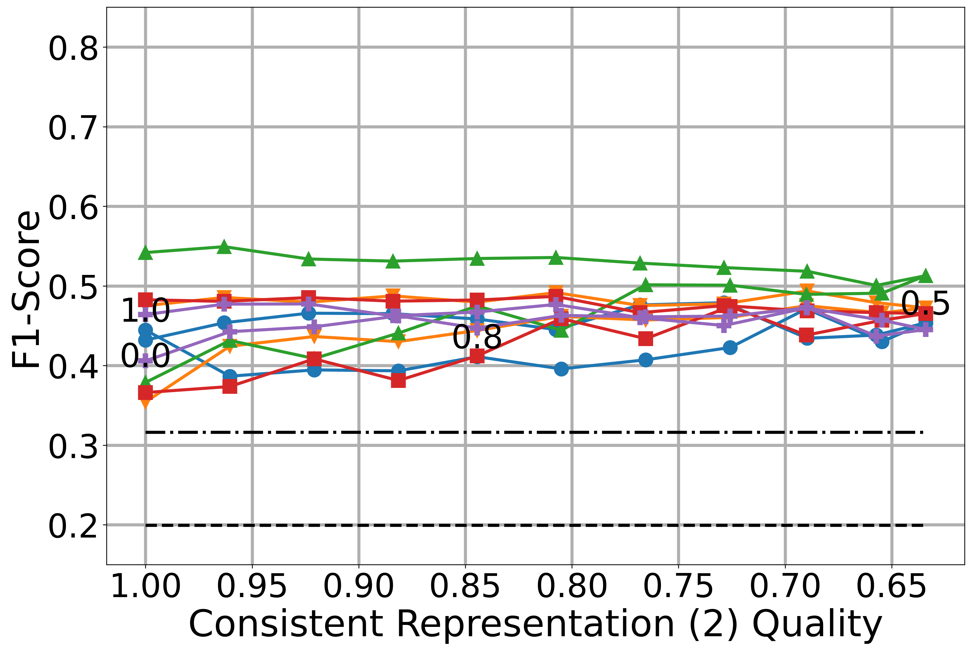
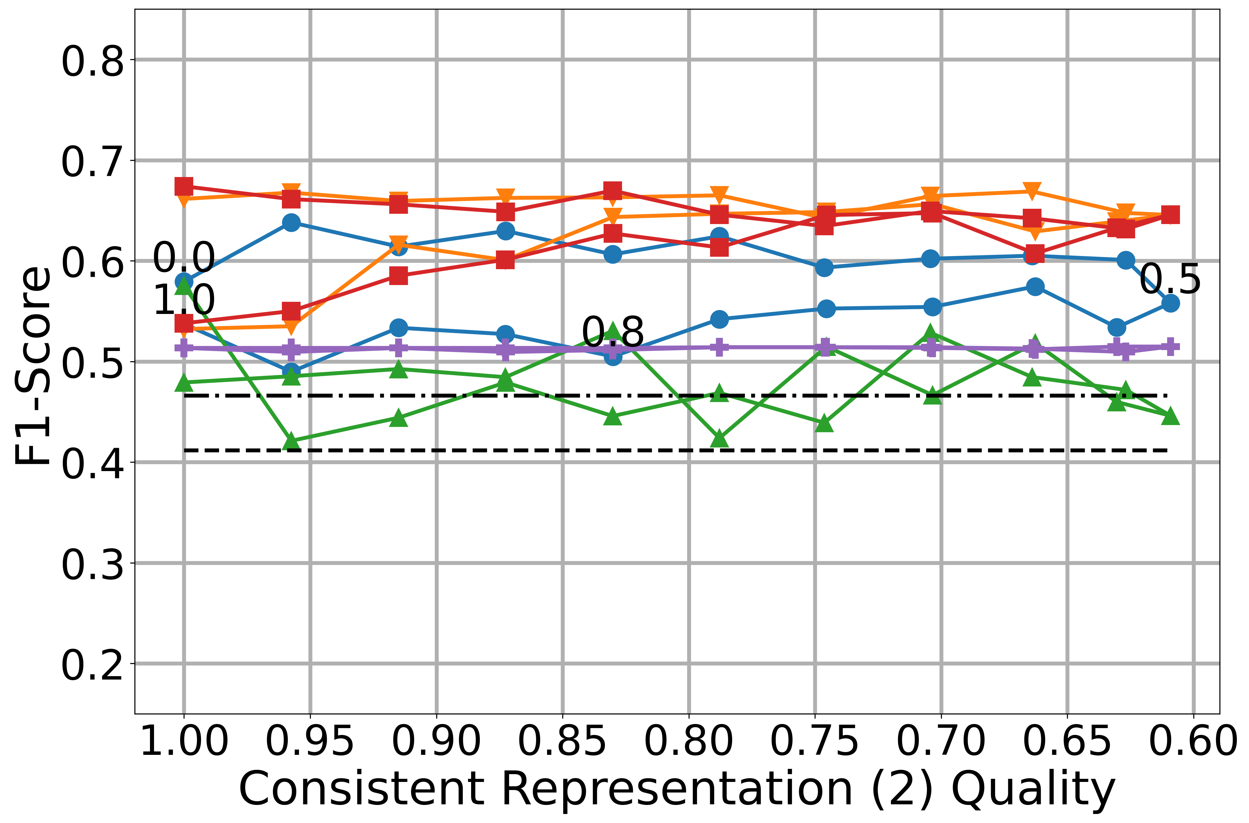
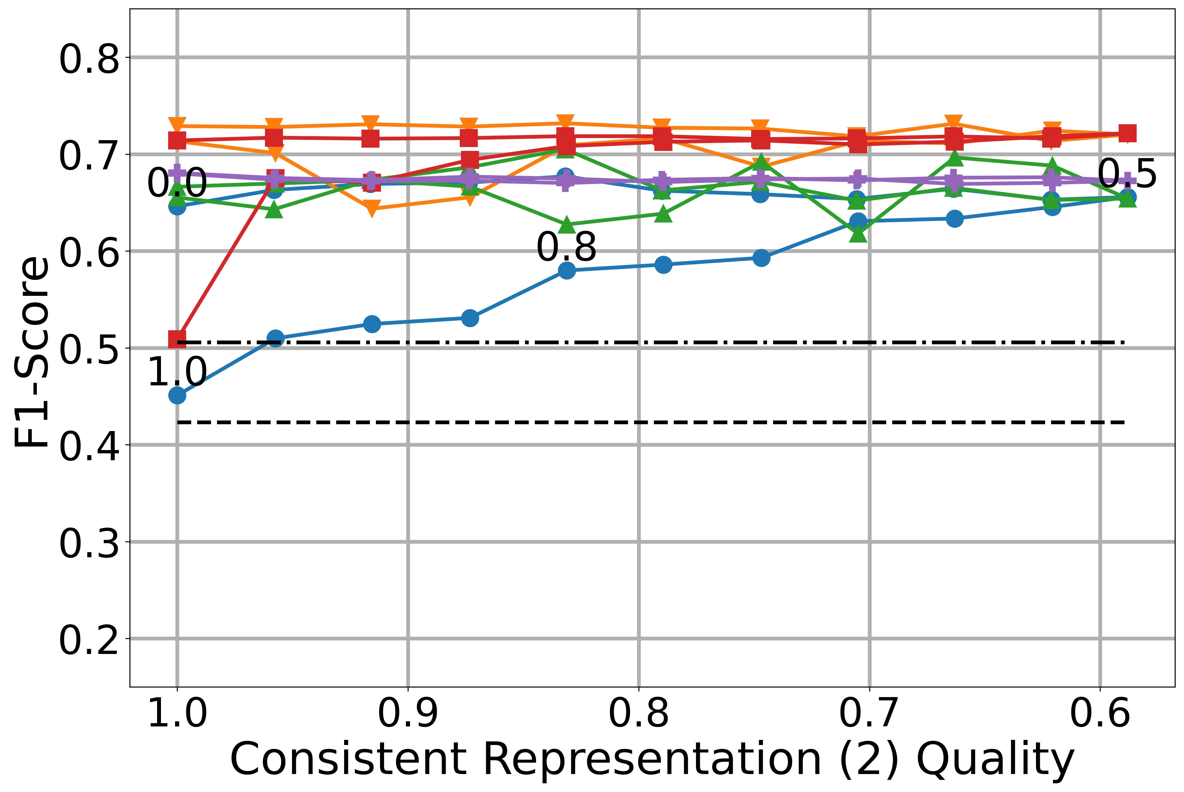
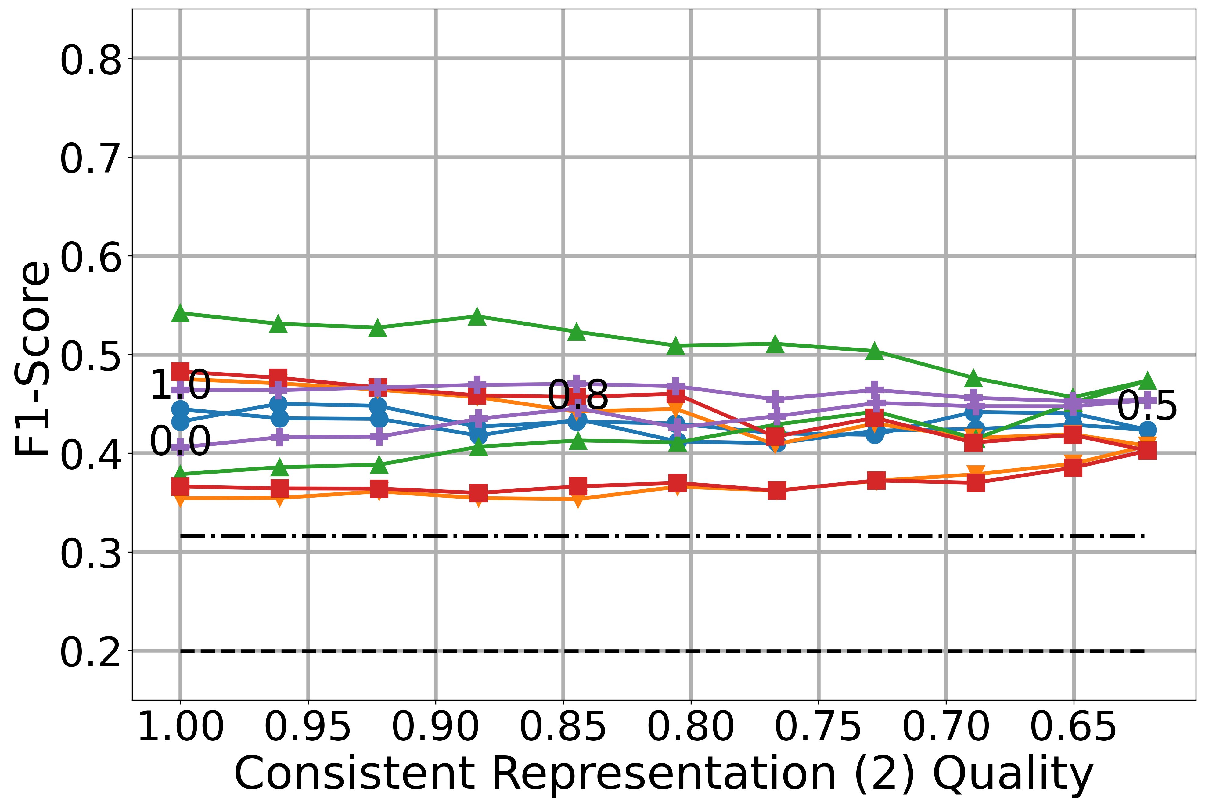
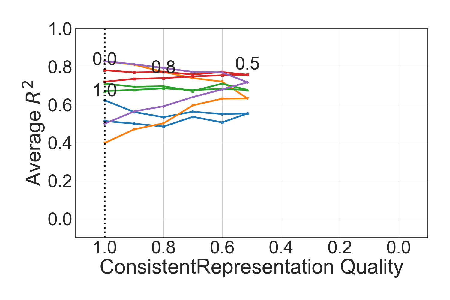
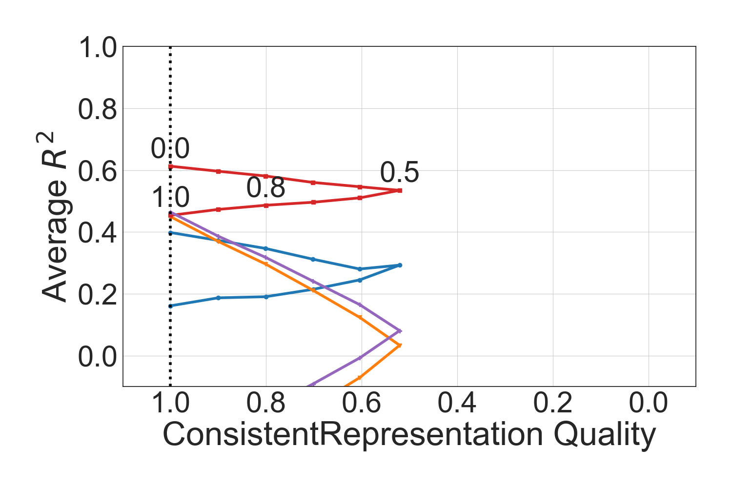
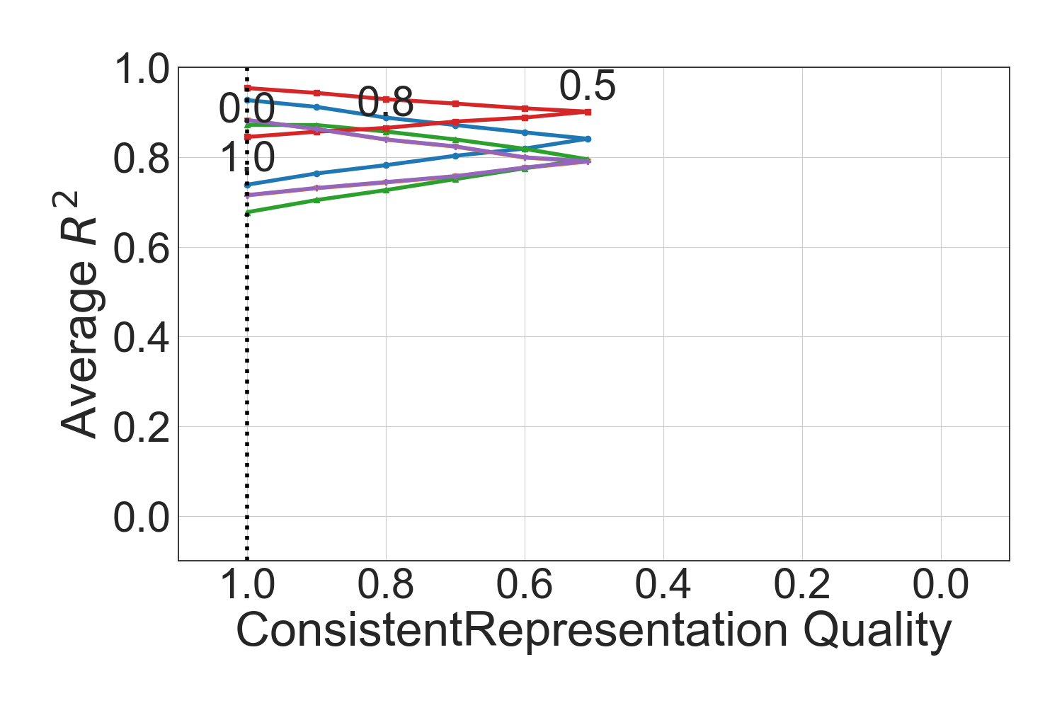
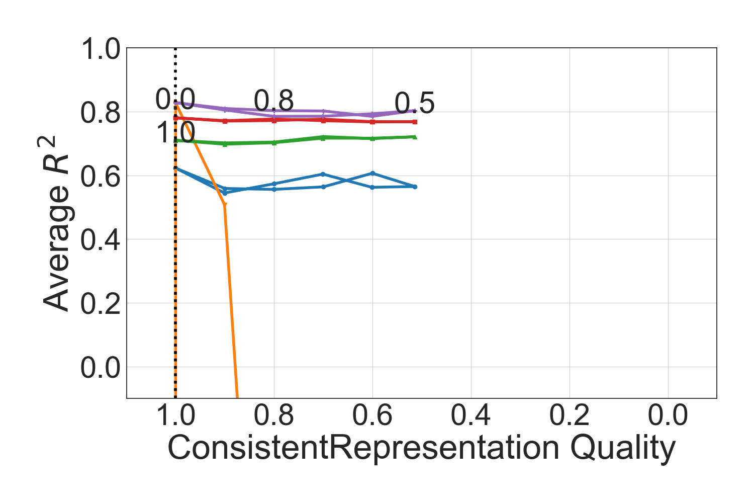
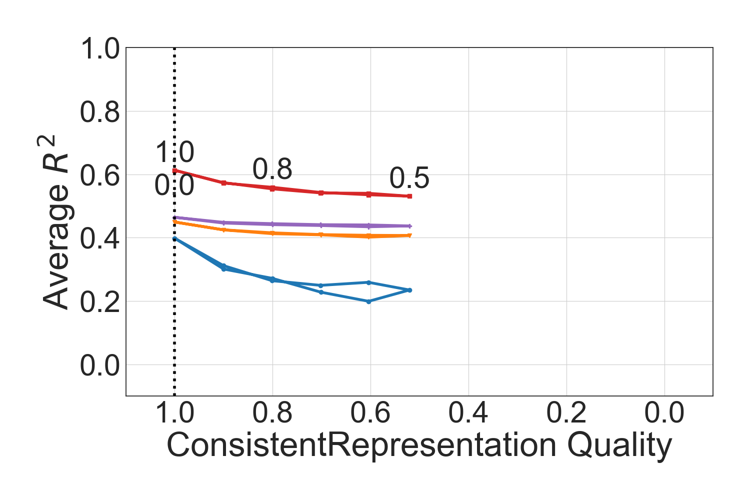
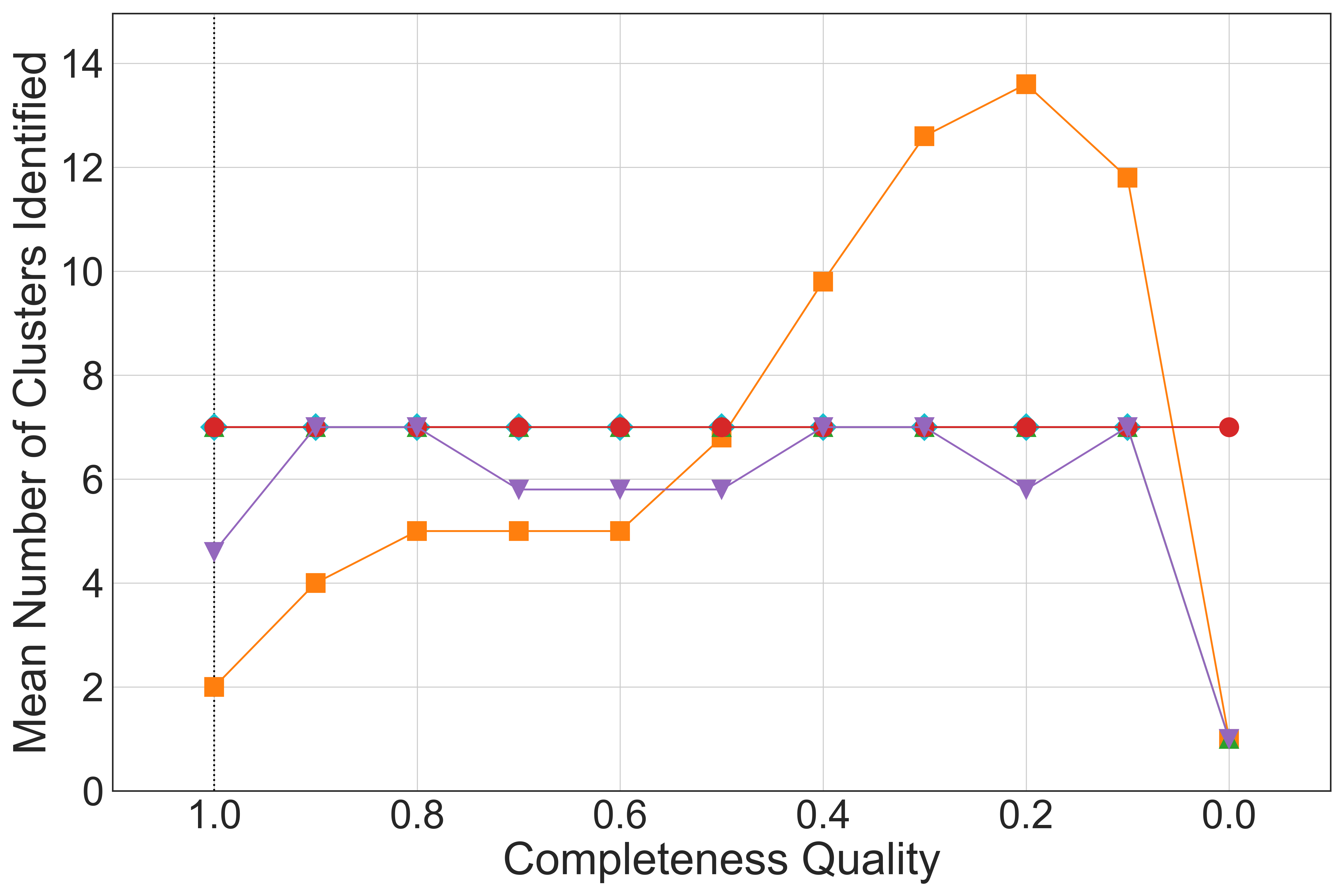
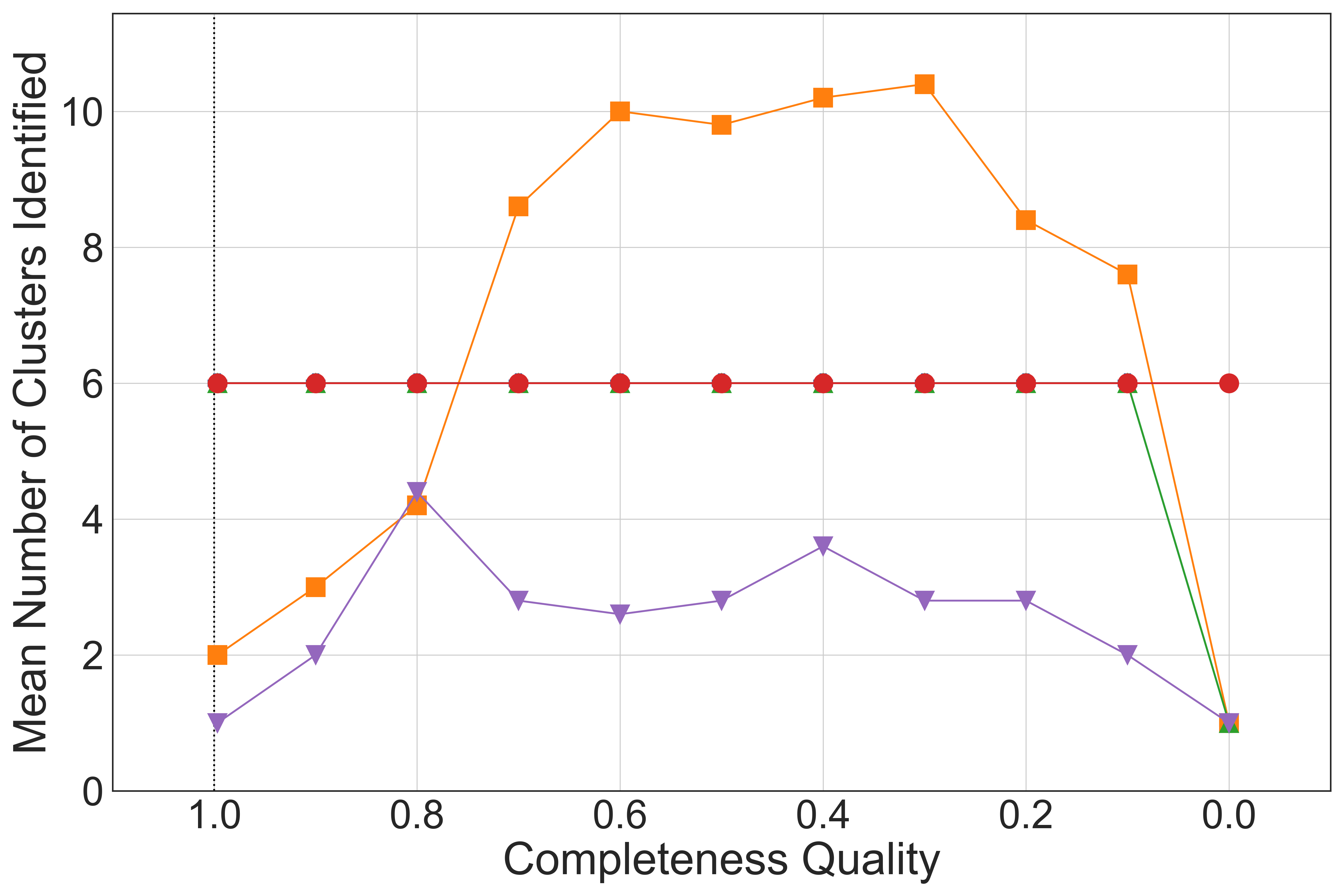
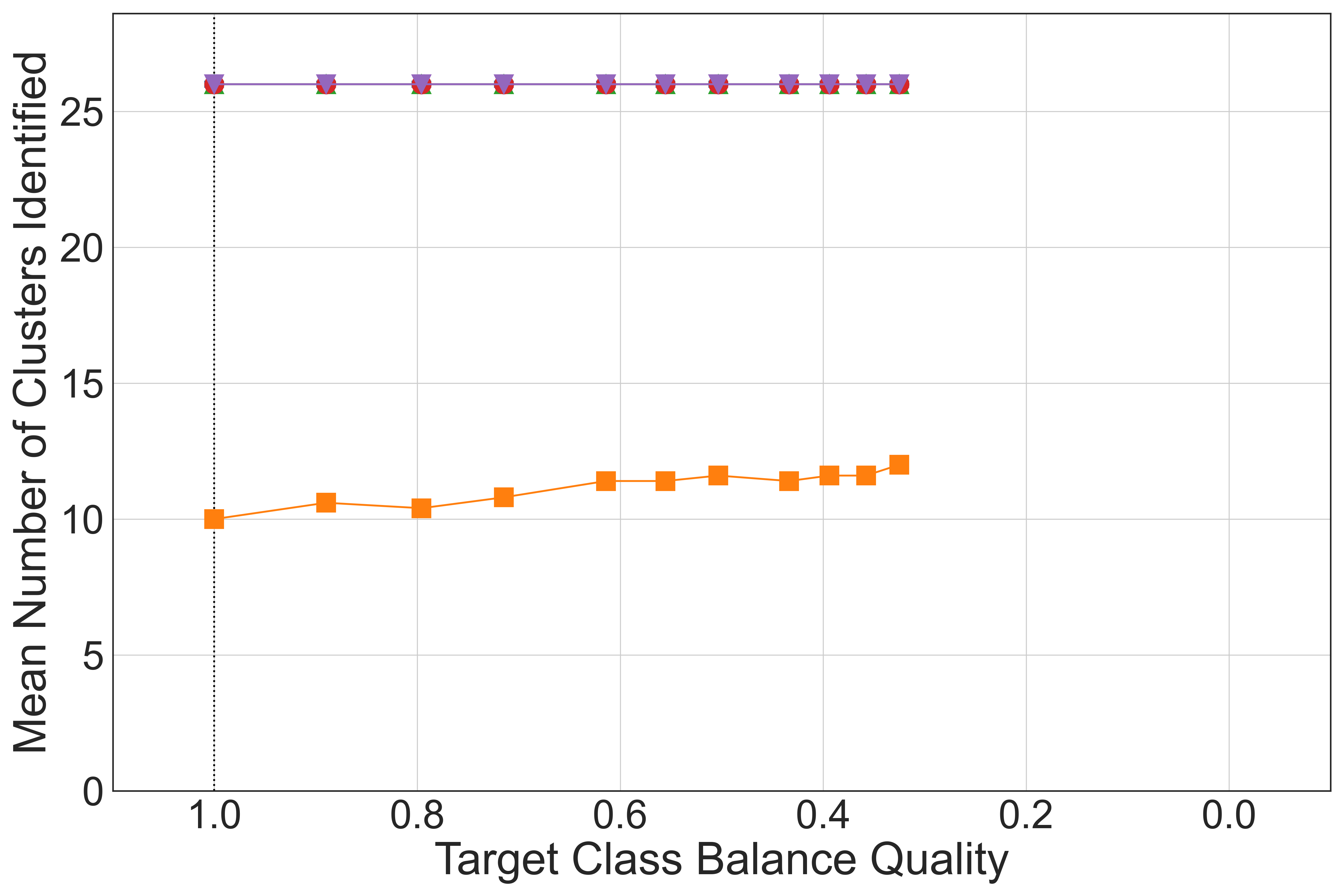
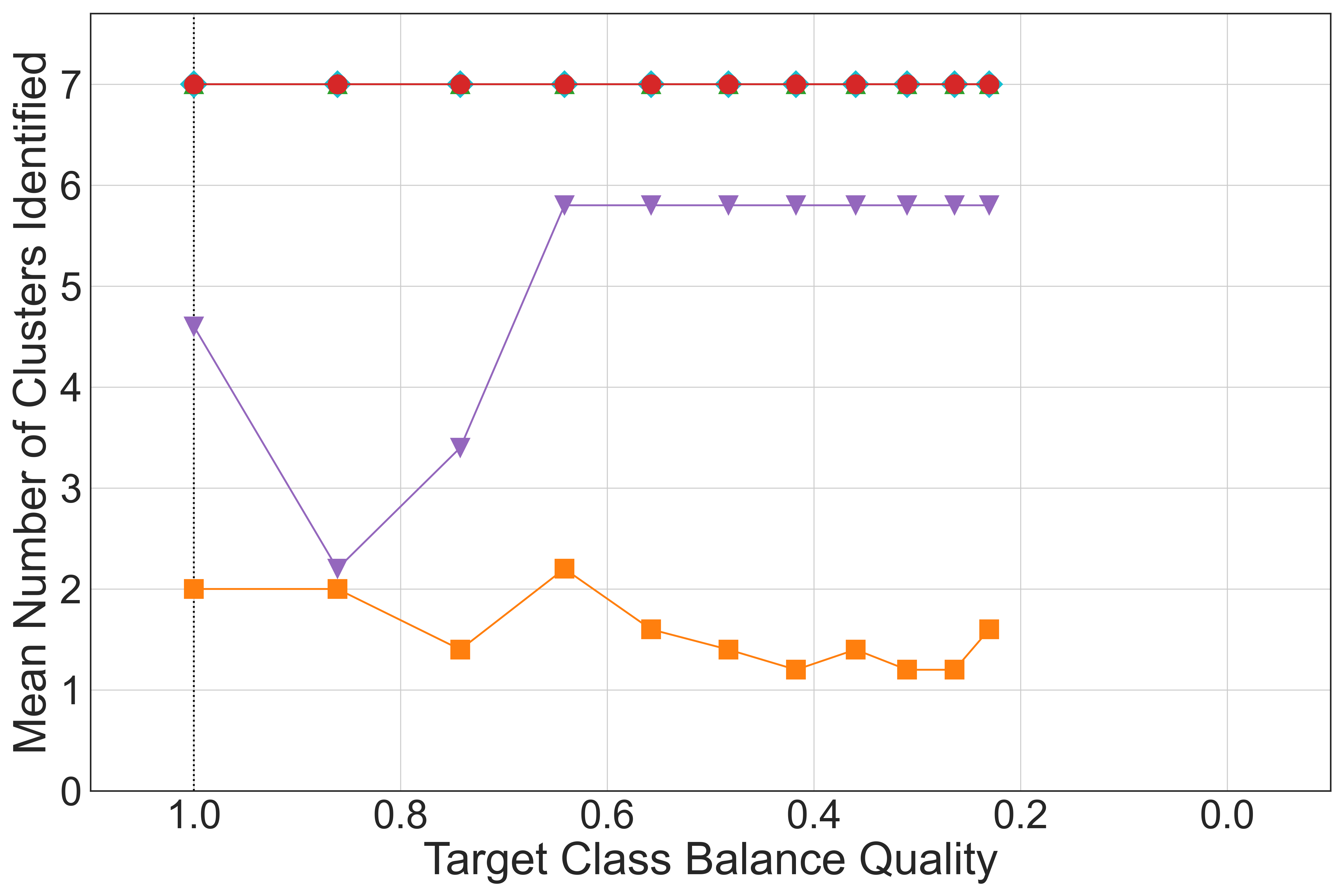
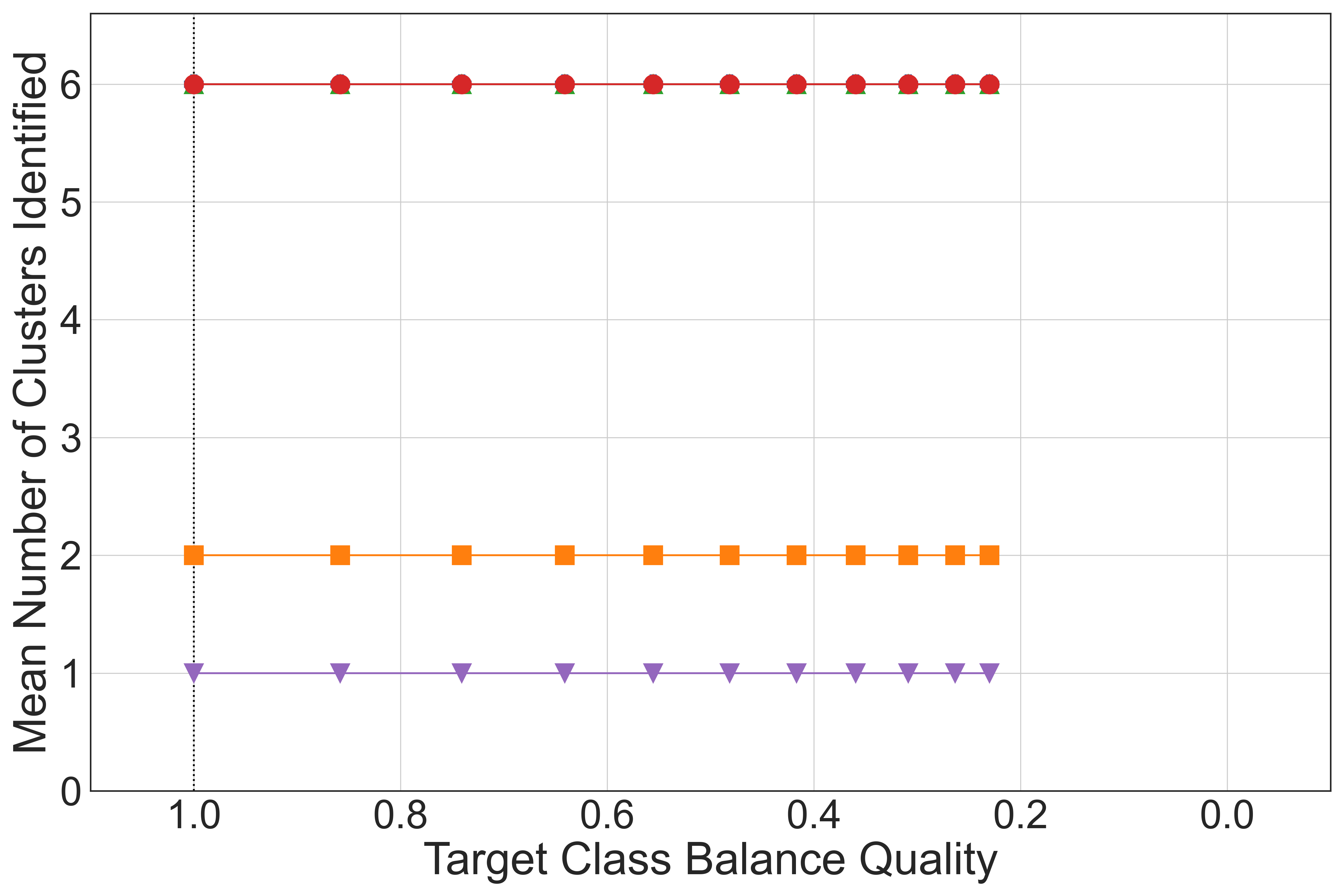
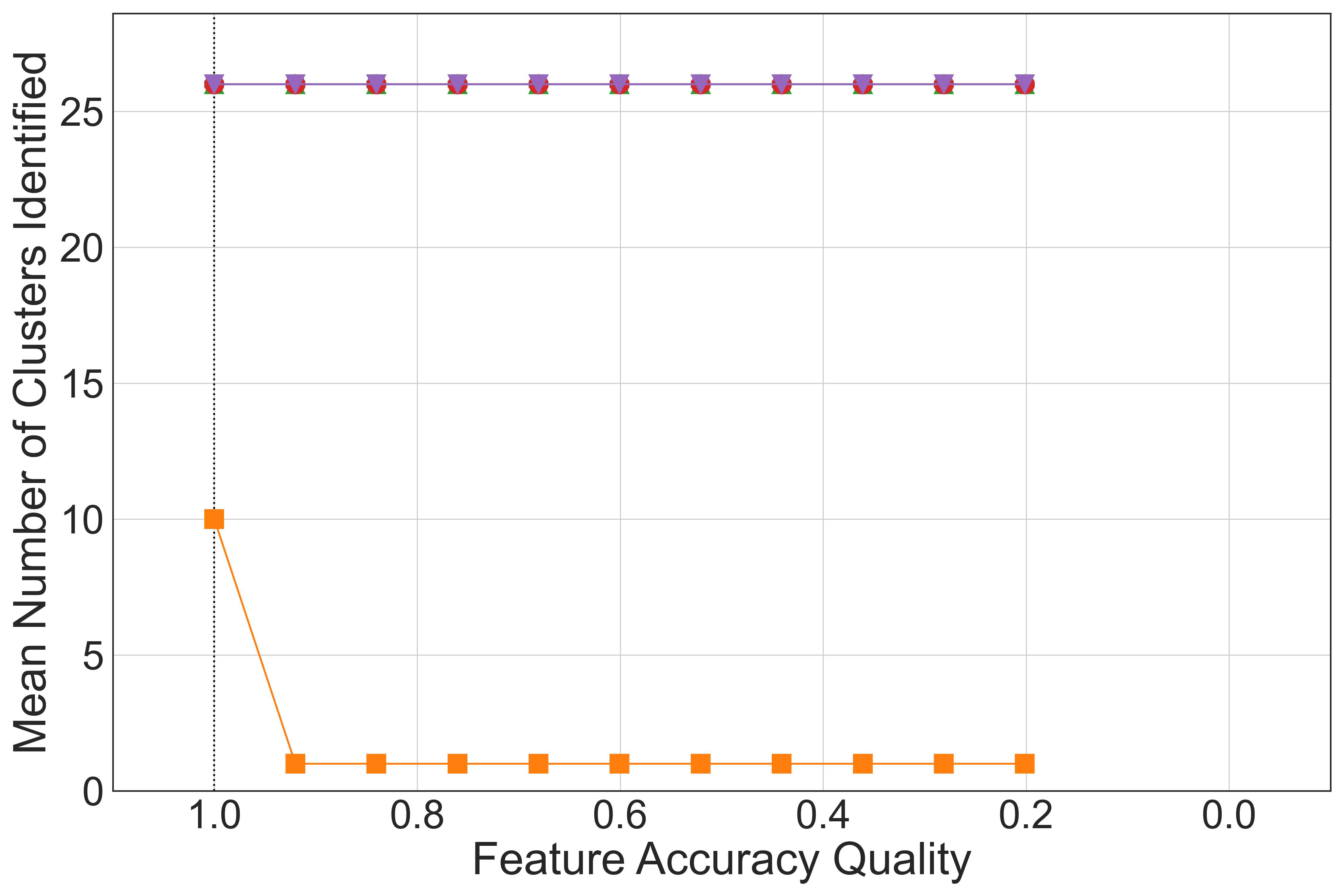
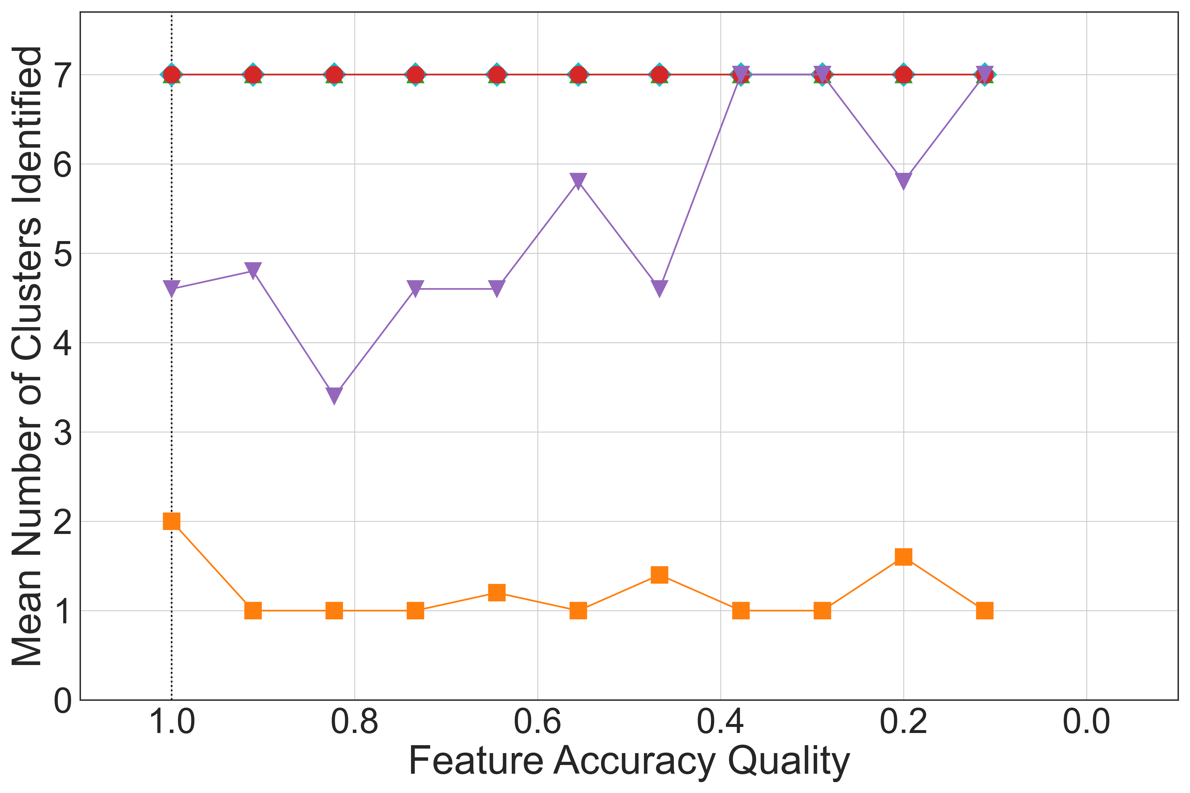
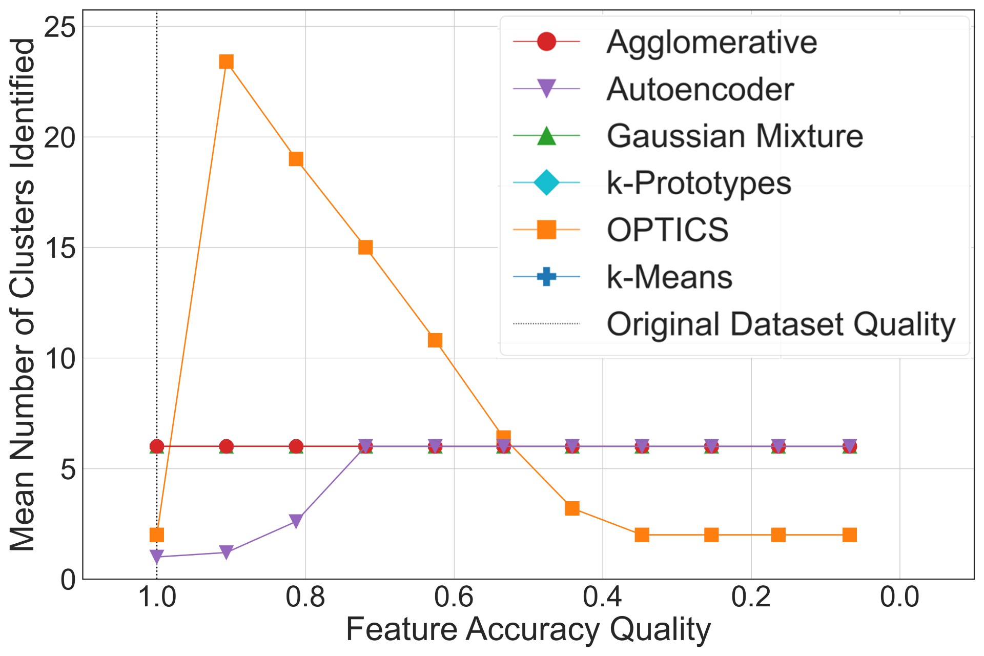
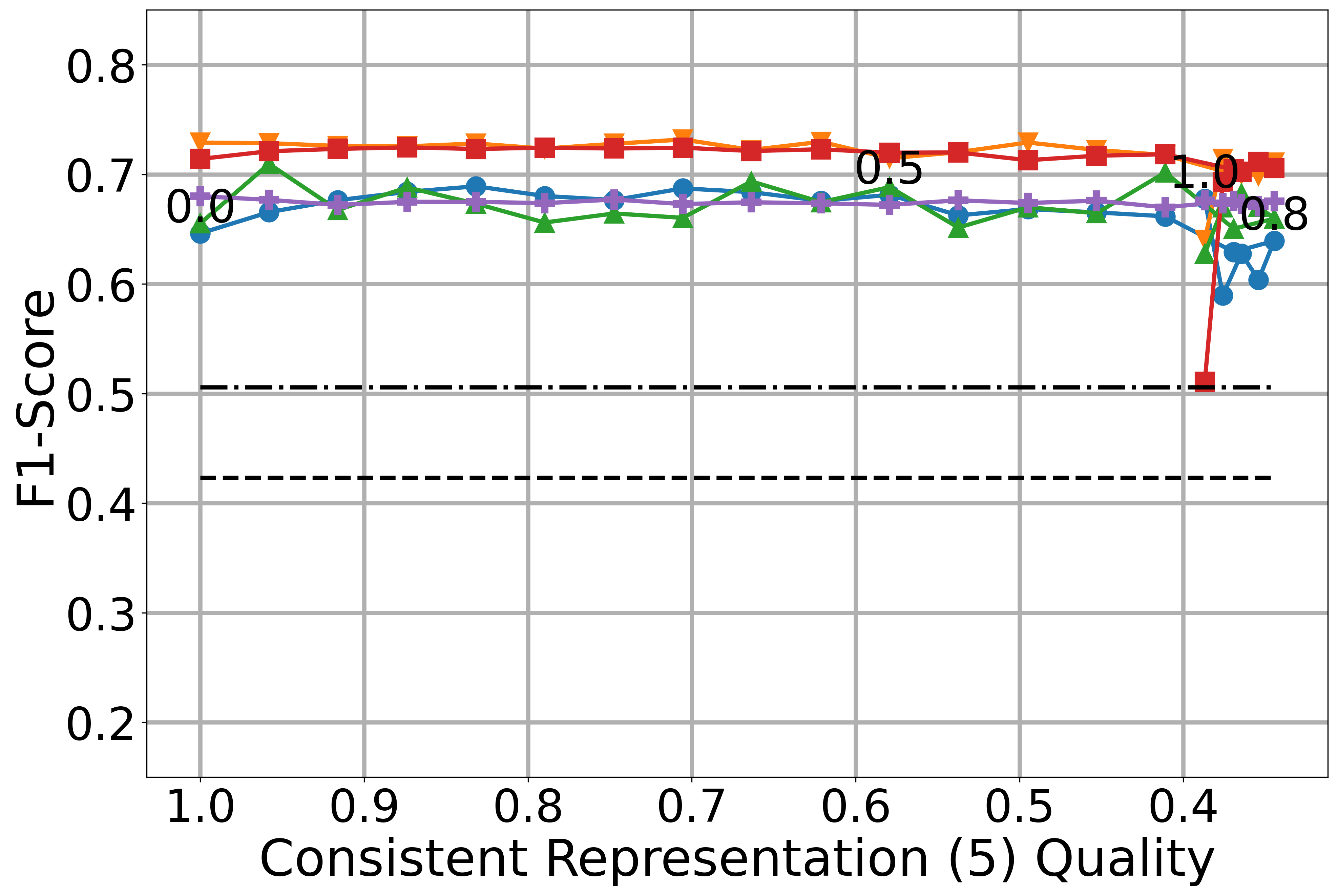
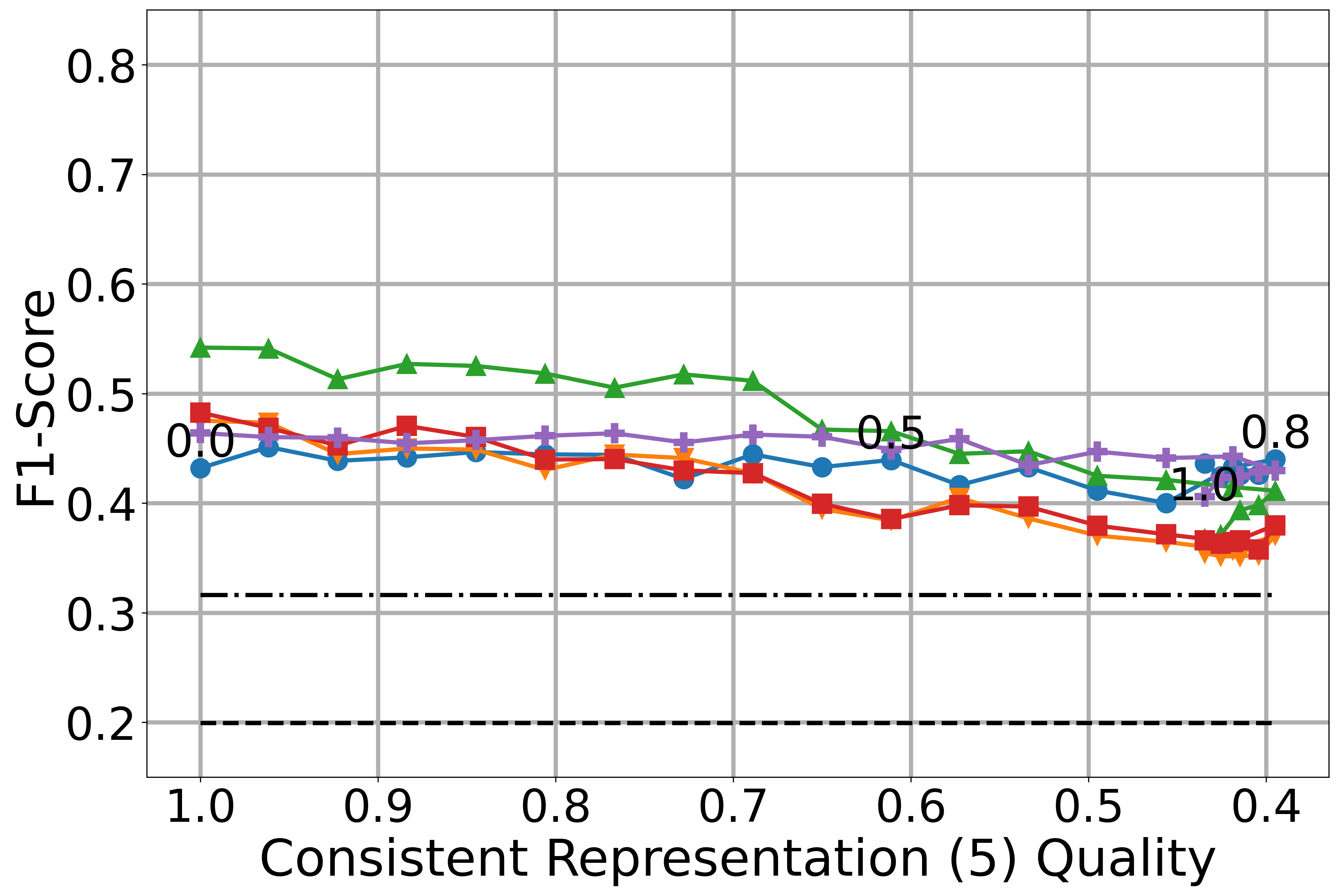
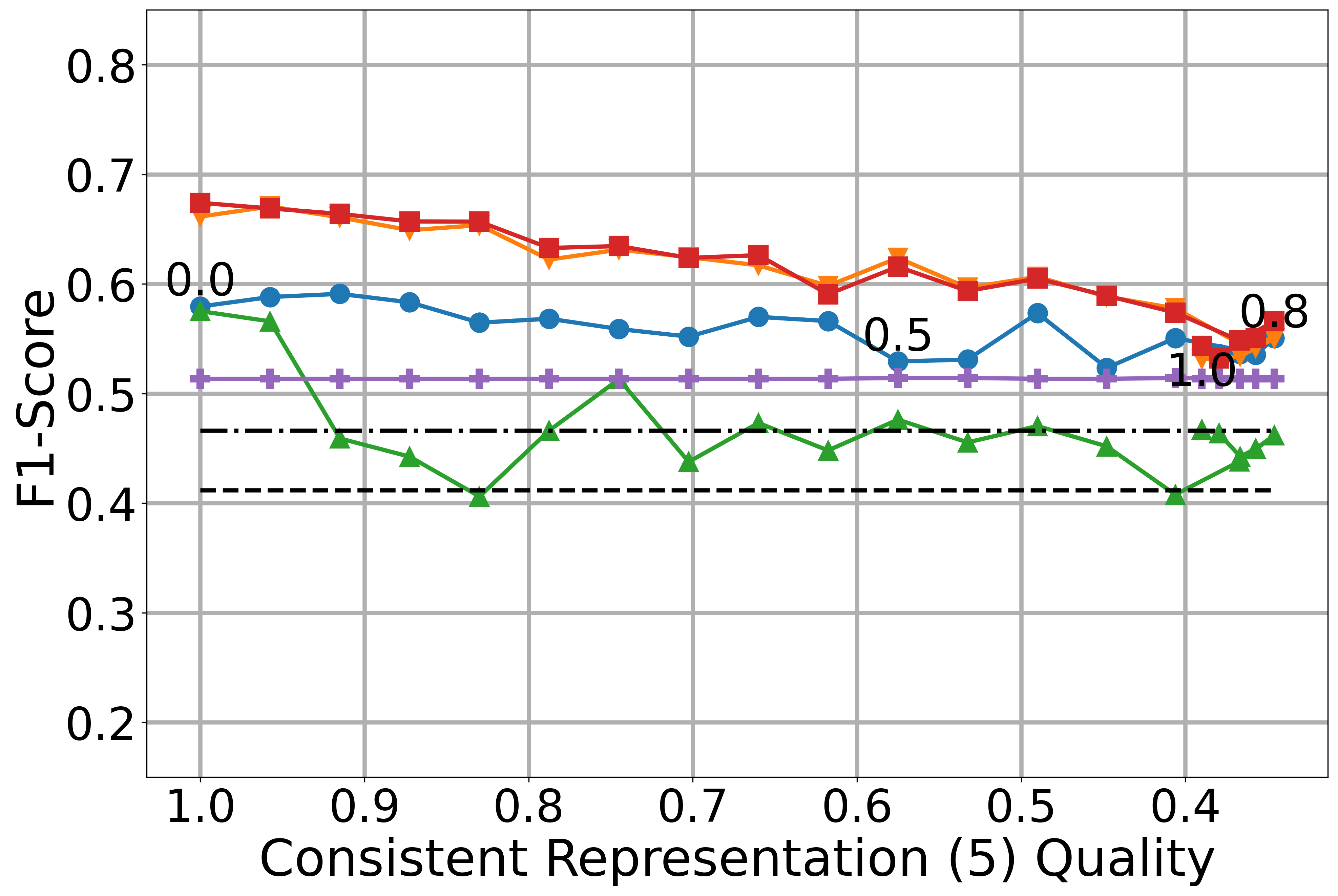
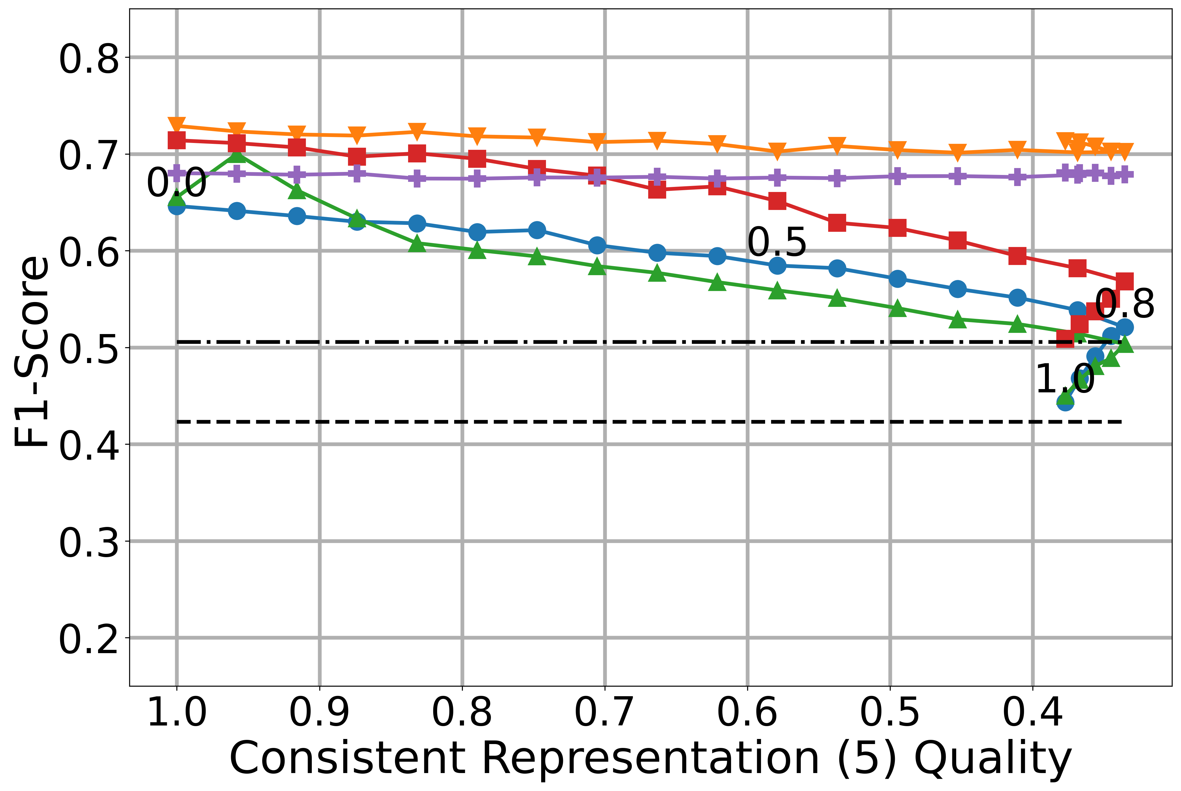
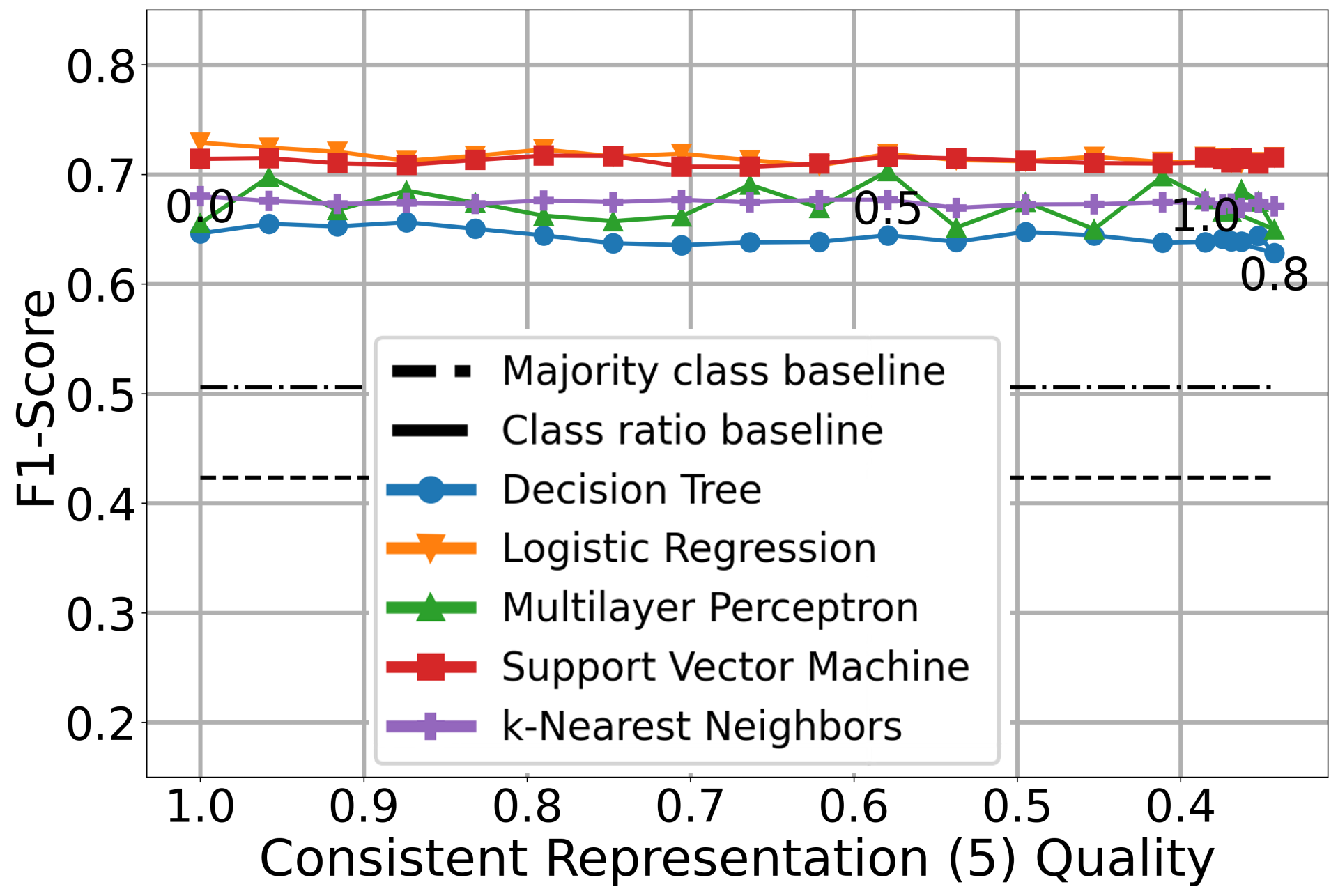
Here, we discuss our observations grouped by ML-tasks and data quality dimensions. For all plots, the horizontal axis indicates the decreasing data quality (training, testing, or both) (Section 3) and the vertical axis indicates the increasing ML-model performance metric (Section 5.5). The quality of the baseline dataset (DQ=1) is indicated by a dotted vertical line. For most polluters, the original and the baseline datasets are identical. Otherwise, the quality of the original dataset is indicated by a dashed horizontal line. All values in the plots are an average of five runs for each algorithm per polluted dataset.
For feature accuracy, we plotted the average of the two metrics and described in Section 3.3. Finally, due to the definition of consistent representation (Section 3.1), the data quality could increase again (instead of decreasing) with a higher pollution level. Thus, we add the degrees of pollution in the plots for such cases.
We discuss the results for each of the scenarios introduced in Section 5.2: Scenario 1 – polluted training set; Scenario 2 – polluted test set; and Scenario 3 – polluted training and test sets.
6.1 Classification
We discuss the effect of degrading the six data quality dimensions of three datasets, namely Credit, Contraceptive and Telco, on the performance of five classification algorithms, namely LogR, SVM, DT, KNN and MLP. We include two baselines trained and tested on clean data, namely a majority-class classifier and a class ratio classifier to better understand the behavior of the studied classification models. The first assigs all test datasets instances to the majority class in the training dataset. The latter selects a label regarding the labels’ ratios in the traing dataset. The target accuracy/balance pollution would shift the class ratios of the training data, which is not reflected in the baseline performance because we report only on clean train and test data. Only for Contraceptive, the classifiers are not binary.
Consistent Representation.
Introducing new representations of the categorical values of the training dataset has a limited impact on the performance of the studied classification algorithms on all datasets (see the first and third rows of Figure 5). For Scenario 2, in which the model is trained on original (clean) data and then is supposed to classify polluted “real-world” data, we observe a slight and slow decrease in the performance of all algorithms with the decrease in test data consistency. Comparing Figures the second and third rows of Figure 5, we can observe a better performance when both training and testing datasets suffer from the same inconsistent representations.
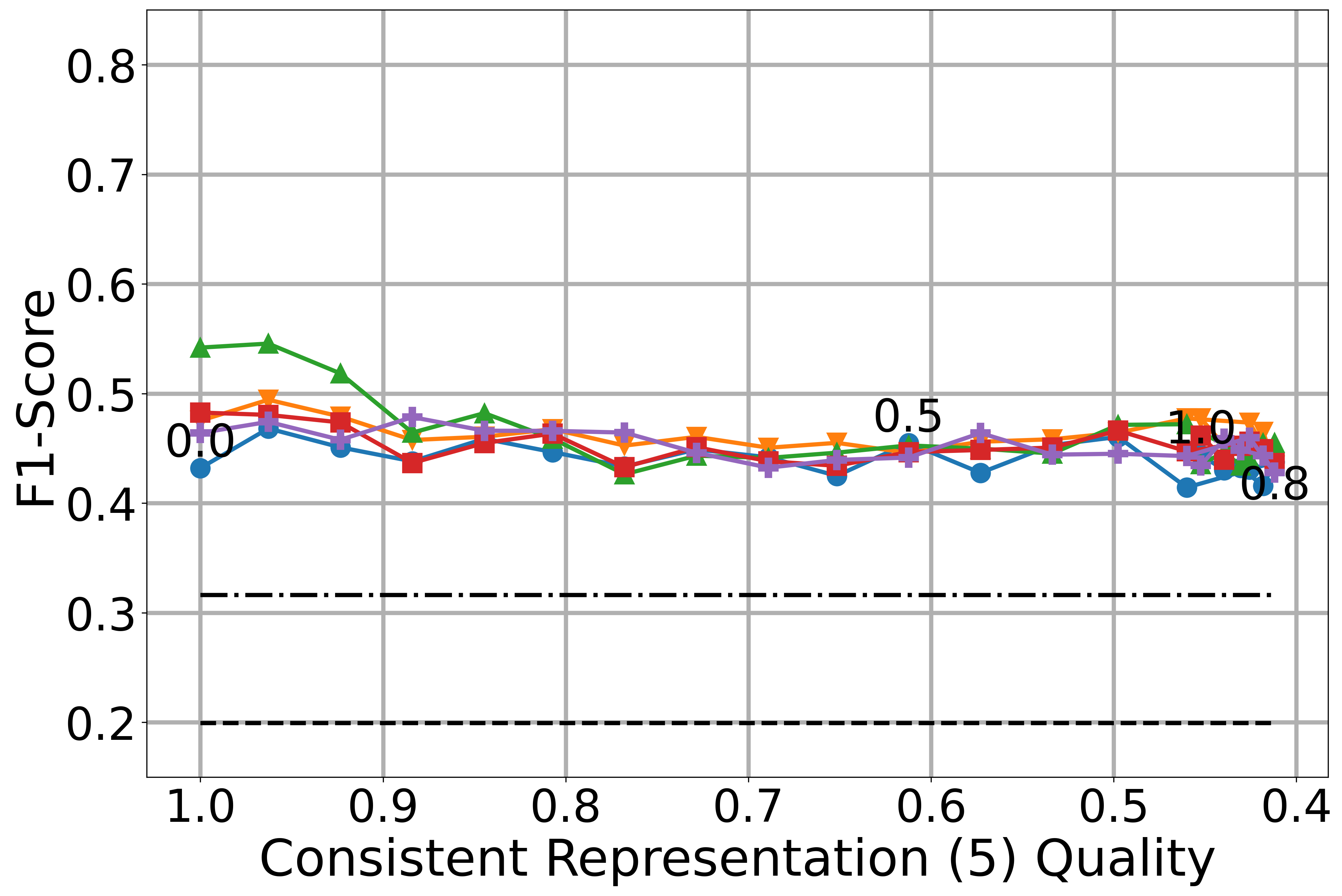
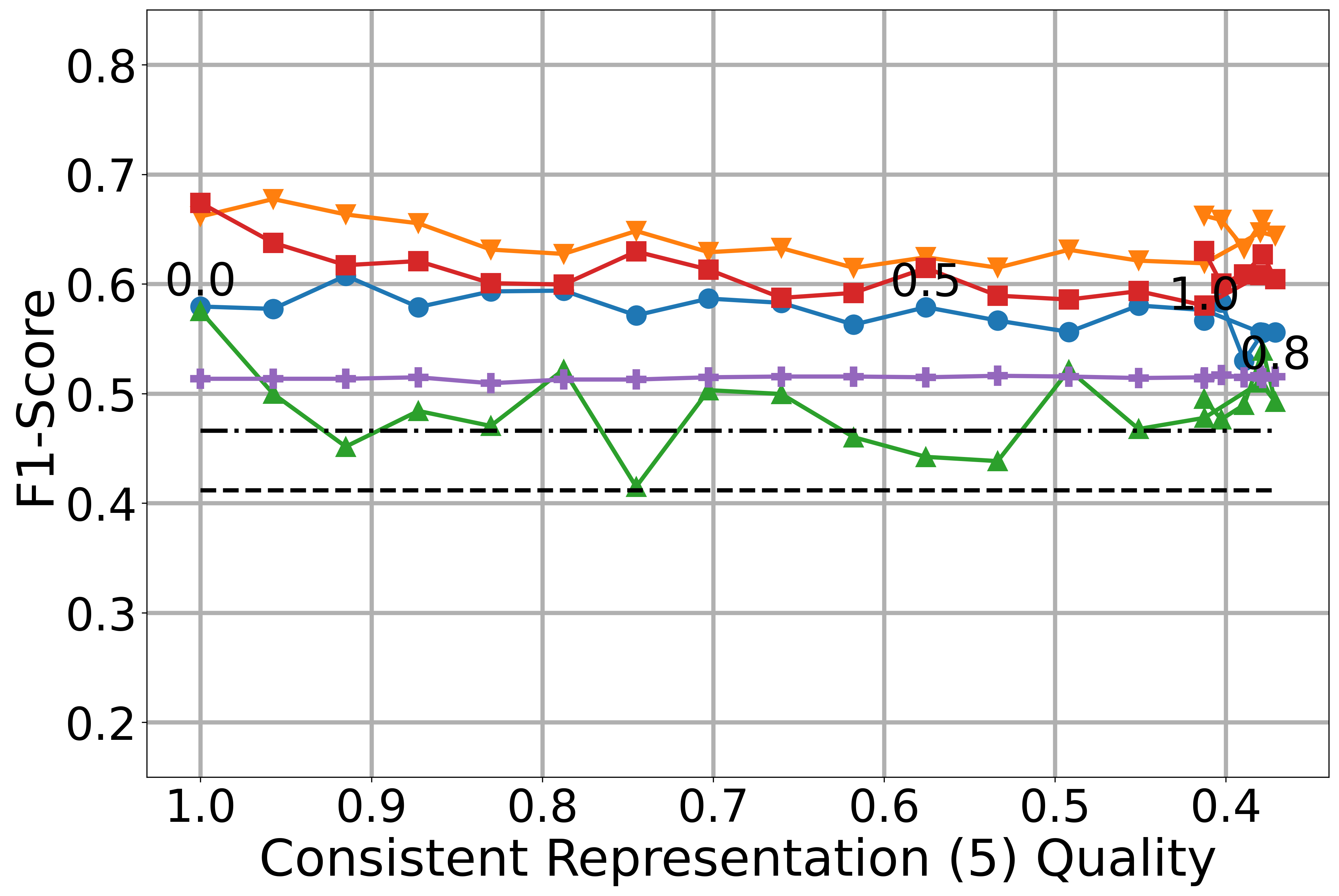
Considering inconsistent representations with only two representations per original value, we note less resilience by some of the algorithm’s and a clear decrease in their performance after polluting 50% of the values in Scenarios 1 and 2 (see Figure 23 in the Appendix).
Completeness.
Our intuition was that compromising the completeness of the training data in Scenario 1 leads to classifiers that are more and more biased towards the imputed placeholder values due to their sheer number. The first row in Figure 6 show a surprisingly limited decline in , suggesting that the models are affected but not biased. The only exception is the SVM model on Telco, which drops drastically in performance once we pollute more than half the dataset, as we see in Figure 5(c).
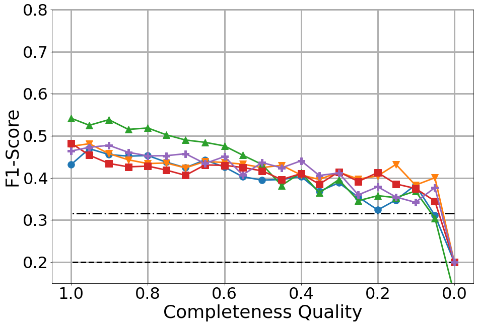
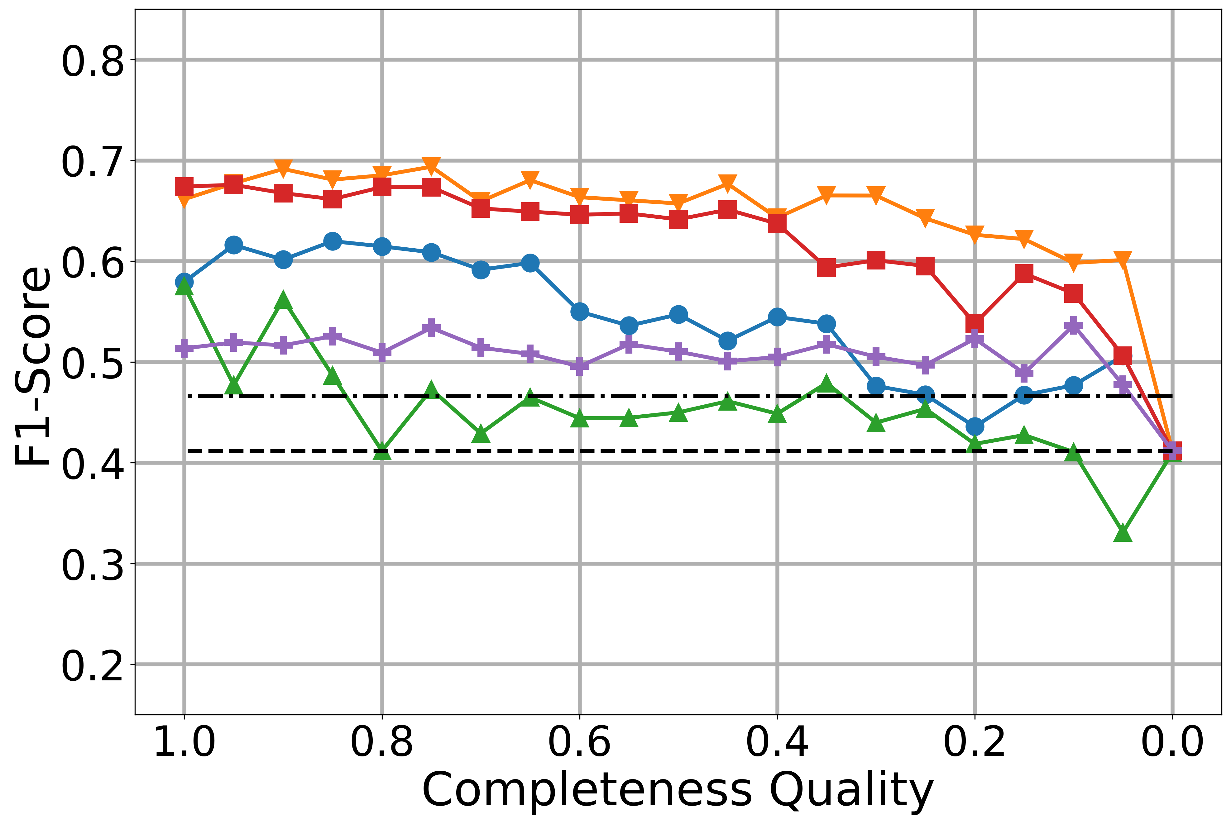
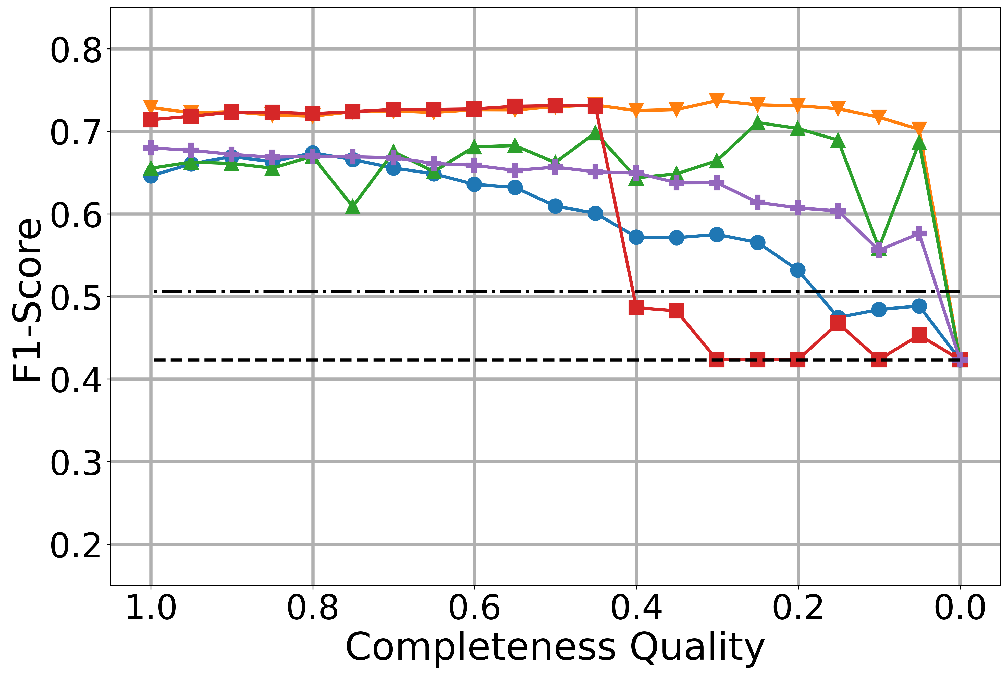
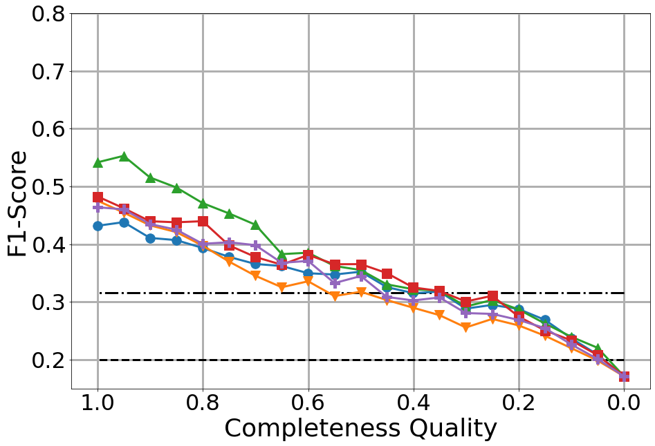
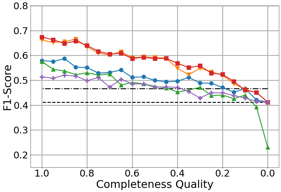
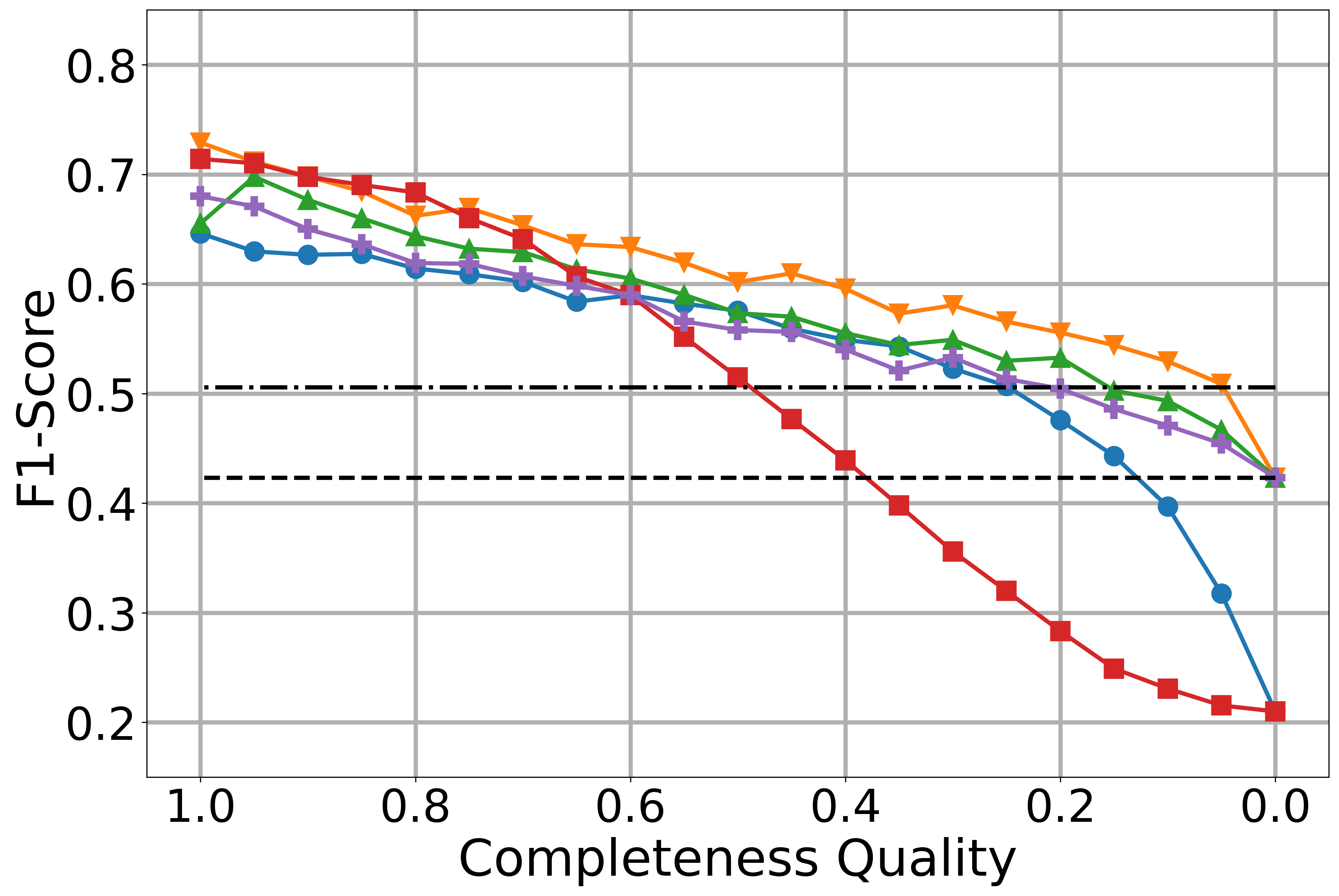
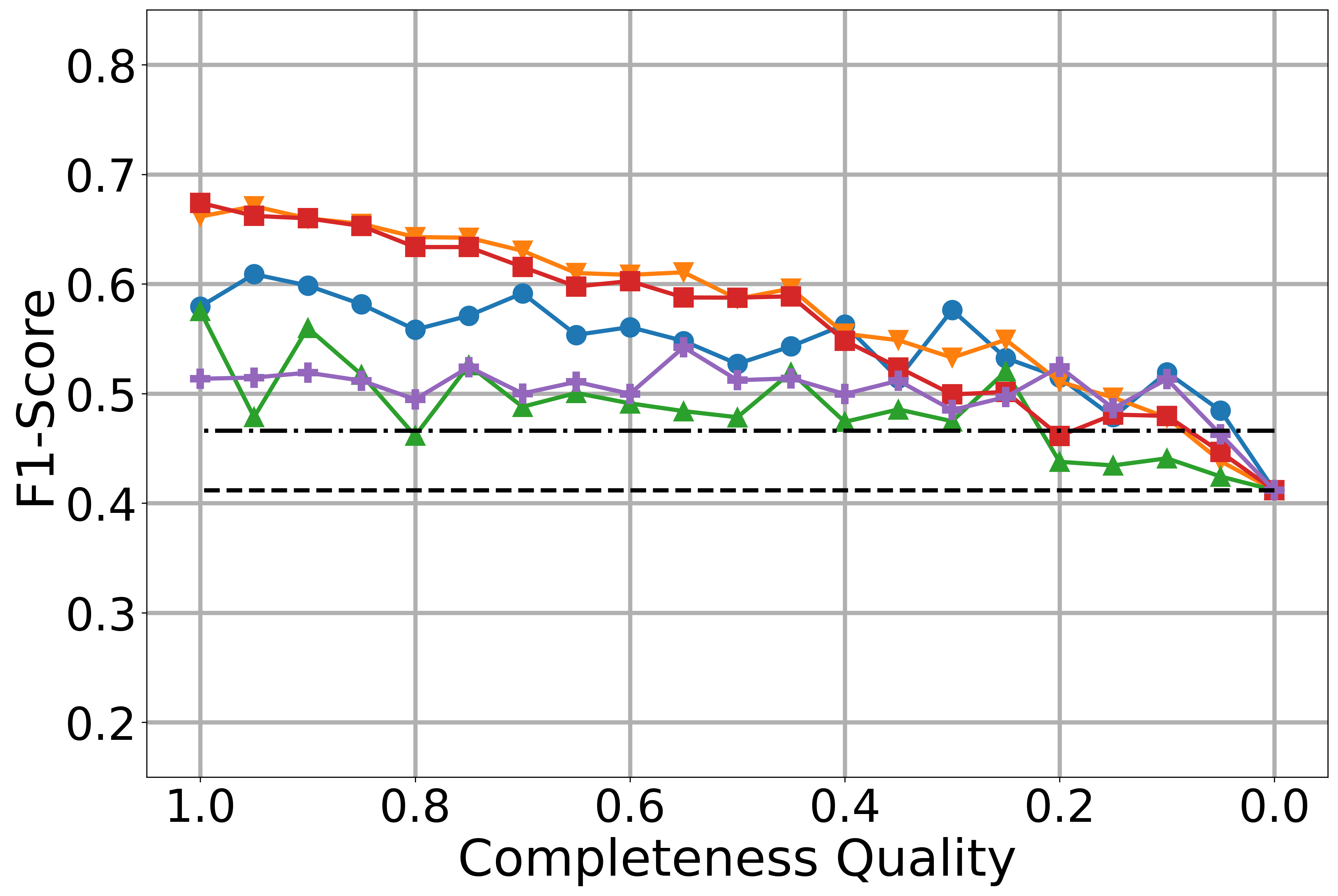
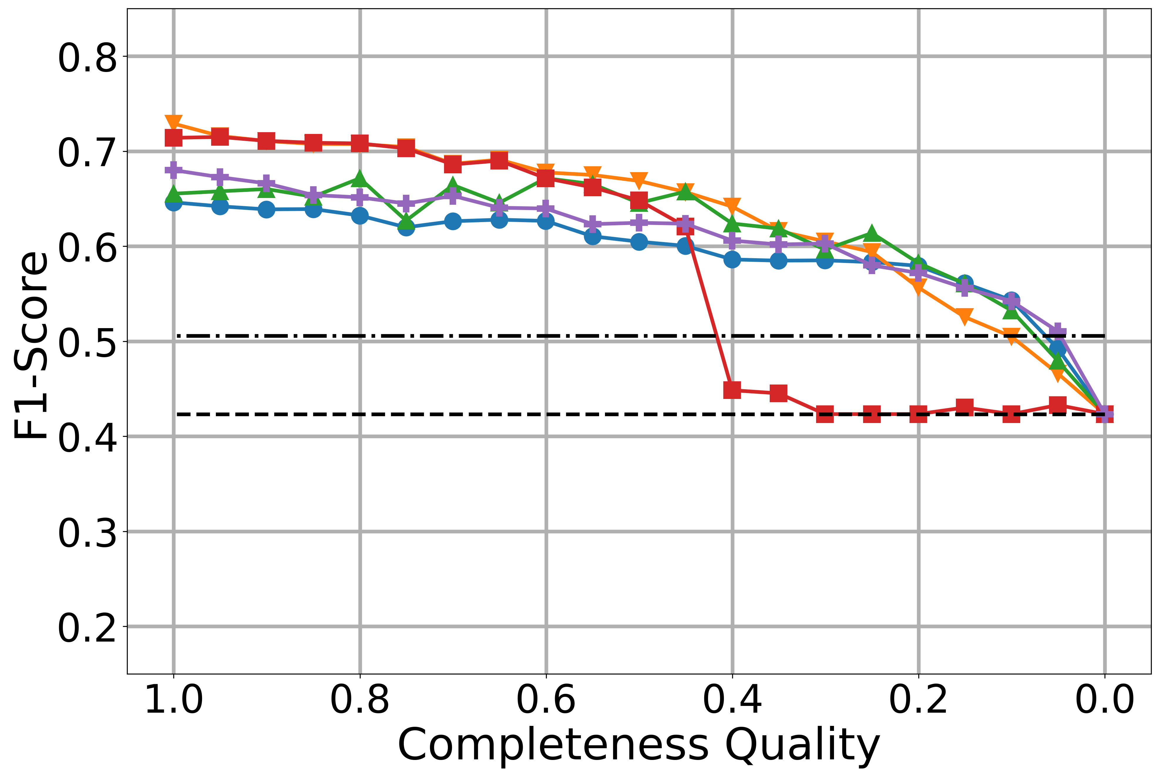
In contrast, in Scenario 2 (shown in the second row in Figure 6), the degradation in prediction performance is faster and ends below the performance of the majority class baseline. Comparing the results of Scenario 3 to the other scenarios in Figure 6, we notice that the risk of classifying incomplete serving data seems to be less if the training has already been carried out on incomplete data.
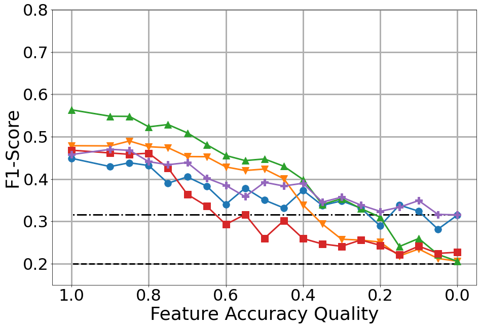
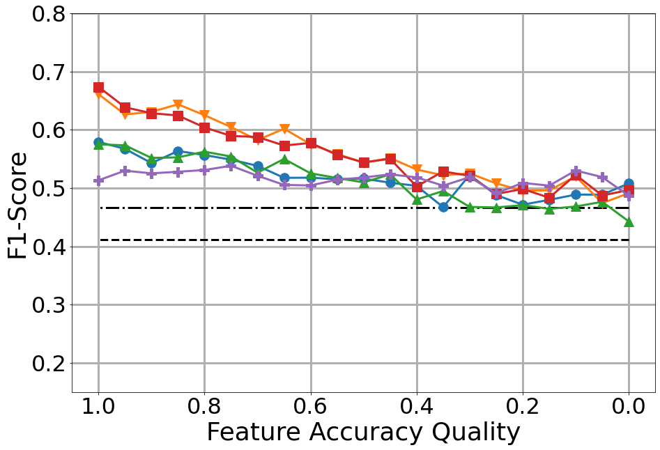
Feature Accuracy.
Training the classifiers on noisy data in Scenario 1 has a non-negligible impact on their performance that varies by the dataset as we can see in the first row in Figure 7). For Contraceptive (Figure 6(a)), the algorithms show a certain robustness until the quality reaches a threshold of 0.8, where the performance degrades more steeply and eventually falls below baseline performance between a quality of 0.4 and 0.2. A similar robustness can be noticed for Credit in Figure 6(b), except for MLP, which performs much worse (10% drop in -score) after introducing only a small amount of noise to the features. Figure 6(c) shows an interesting pattern: The linear models (SVM and LogR) seem very robust to degrading feature accuracy up to a certain point, where they suddenly lose performance rapidly until they meet with the majority class baseline. The differences in the datasets do not allow us to make general statements besides that initial robustness. For more insights, one could investigate the influence of the separate feature accuracy qualities (for categorical and numerical values) as the combination of them does not allow us to reason about their individual contribution to the overall loss in performance.
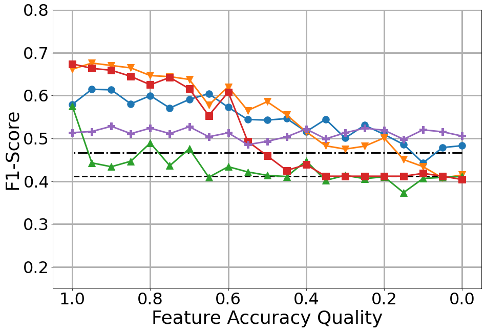
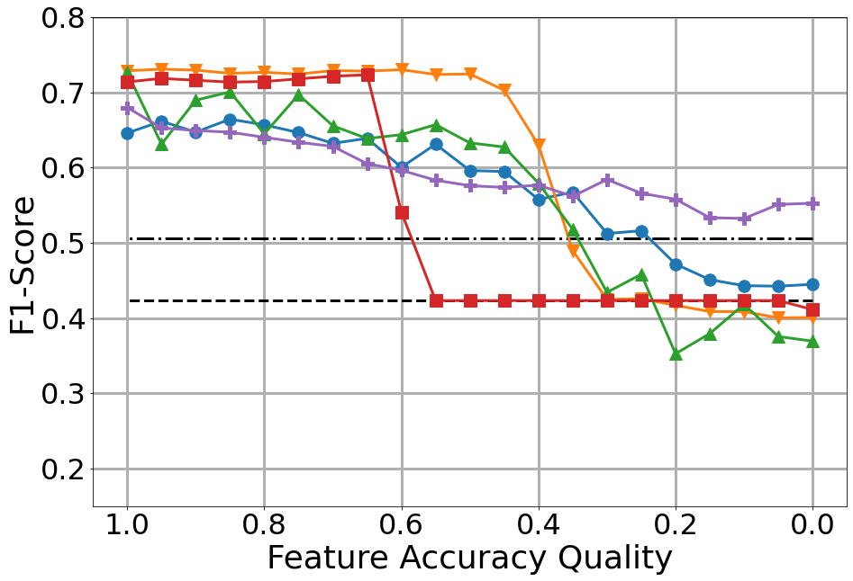
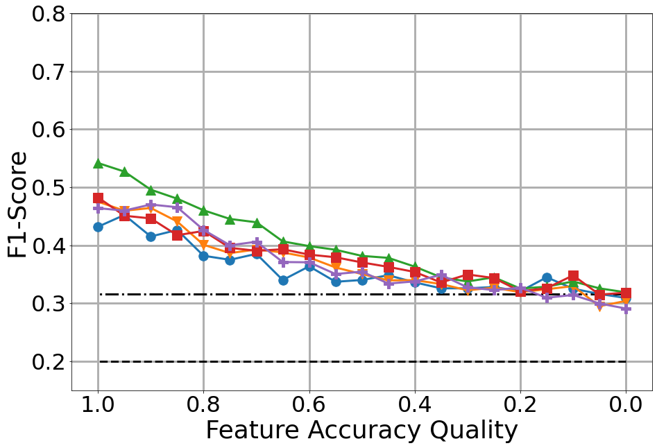
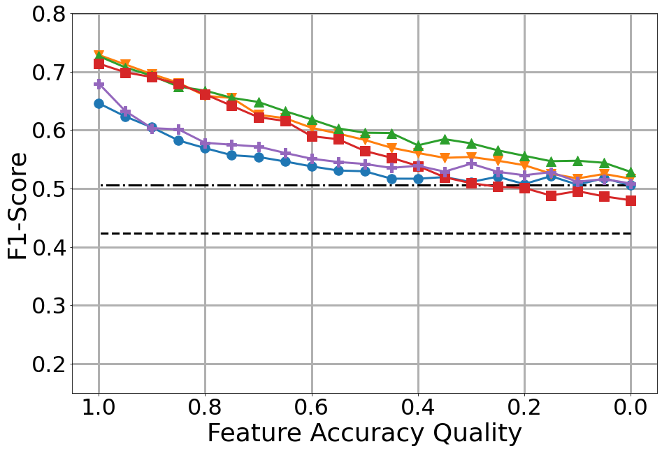
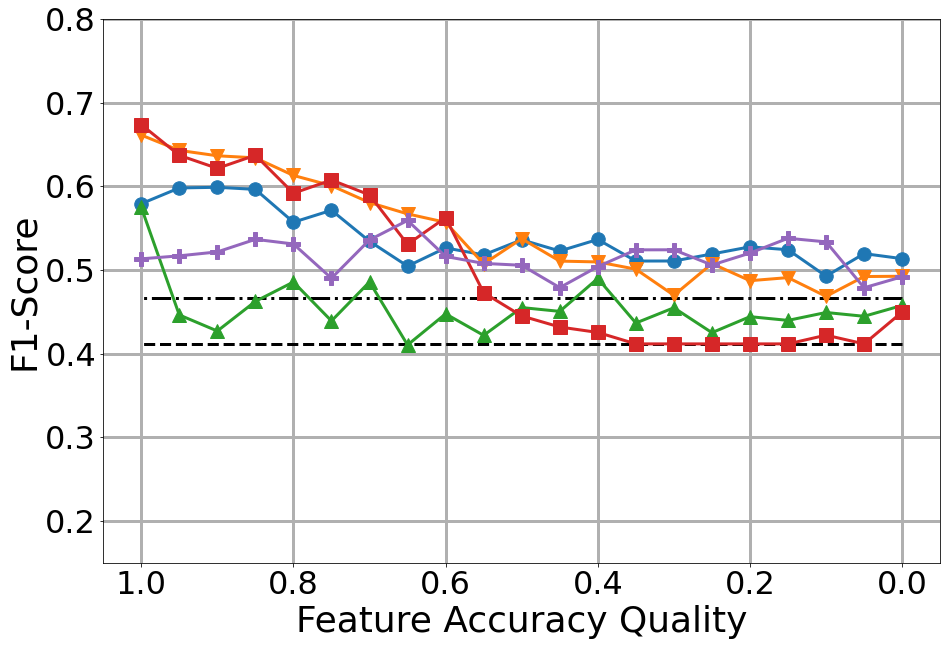
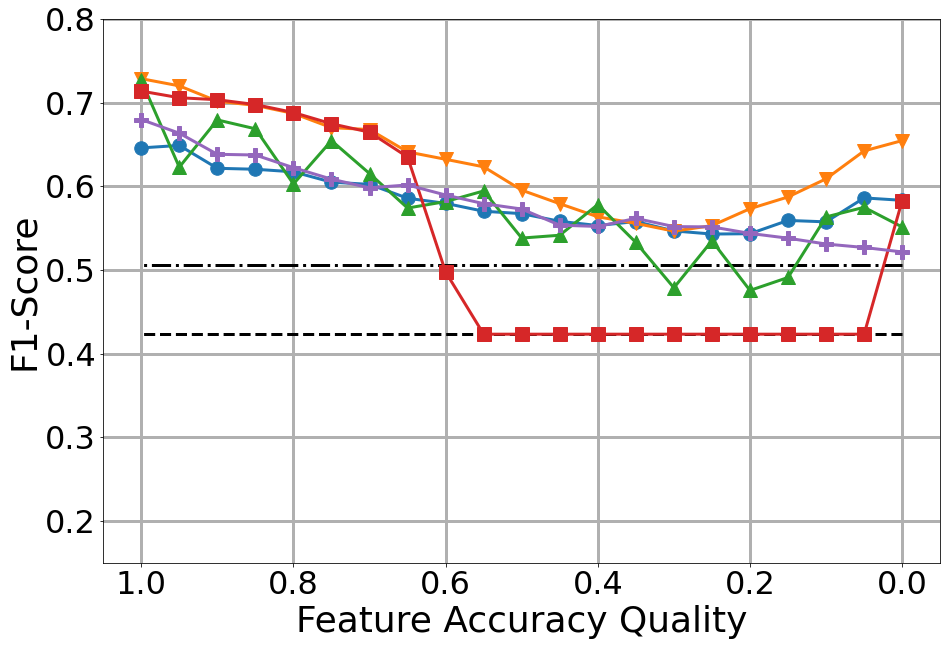
For Scenario 2 where we train on original data and test against polluted data (see second row in Figure 7) , we can see that the performance linearly decreases with reduced feature quality of the serving data, while staying above baseline performance most of the time. There are no significant differences in the relative behavior of the algorithms, as their performance declines with roughly the same slope. Reducing the quality of the serving data to 0.5 causes a drop of about 10% in for the linear models. There is almost no significant difference in performance for the KNN classifier in Figure 6(e) which seems to be a dataset specific finding. Generally, our findings suggest that these algorithms are rather robust against reduced feature accuracy on the tabular data that we tested with. For Scenario 3, we observe a similar behavior as in Scenario 1, but the linear models’ performance appears to improve once we pollute the training and serving data (see first and third rows in Figure 7).
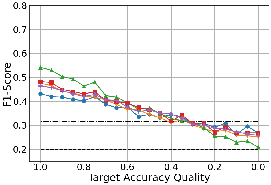
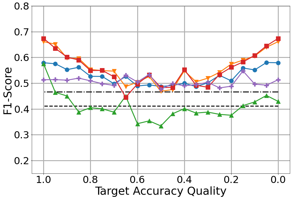
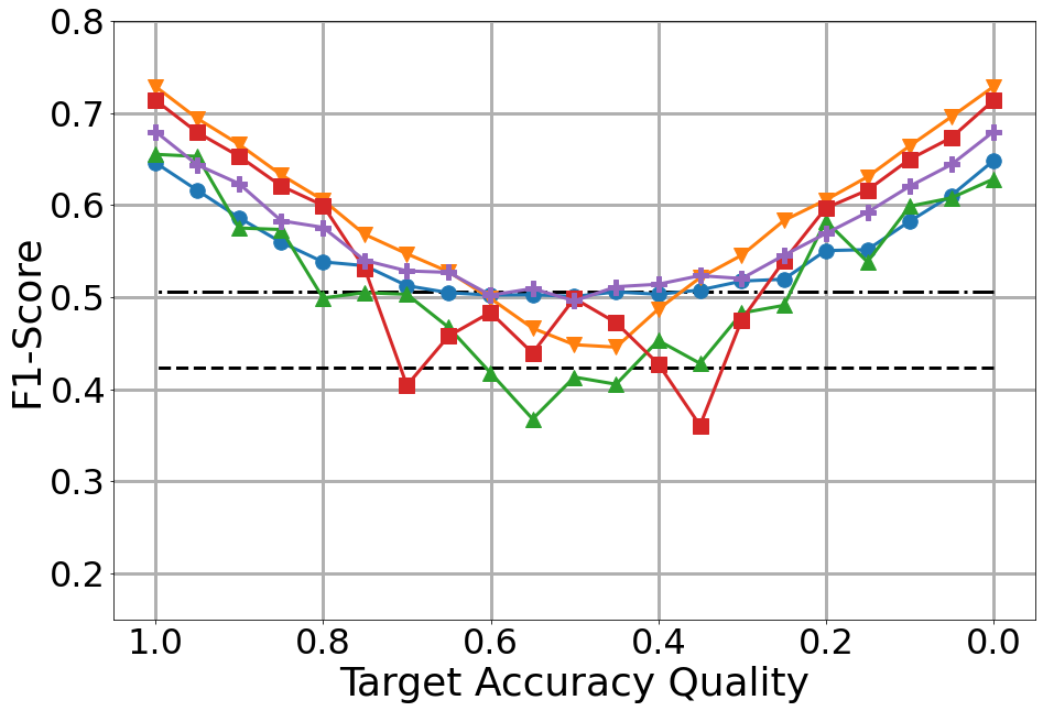
Target Accuracy.
The target accuracy data quality dimension is especially relevant in the classification task, as it simulates labeling errors/noise in the data. Scenario 1 in the first row in Figure 8 could depict a real life situation in which the training labels were collected by crowd workers (noisy and inconsistent) and the test labels were carefully handpicked by experts (as close to the ground truth as possible). Therefore, the results show the connection between labeling errors in the training set and loss in real-world performance of the classifier. For Scenario 1, there is almost a linear decline in performance for Contraceptive and Credit in response to decreasing the training dataset target accuracy, as we can see in Figures 7(a) and 7(b). Telco shows in Figure 7(c) a different behavior for the linear models, which steeply decline in performance around a target accuracy of 0.5, while the other models follow a more linear pattern.
For all the datasets and all algorithms, we found that once the target accuracy of the training data is equal to or worse than 1 divided by the number of classes, then the prediction performance is below that of the class ratio baseline classifier. In addition, we note that up to 20% of training labels could be flipped without a performance’ losses of no more than 10% in -score for most of the algorithms. The performance of the MLP and SVM in Figures 7(b) and 7(c) also showed a very high variance across the five different seeds, which indicates that they are the most sensitive to incorrectly labeled samples.
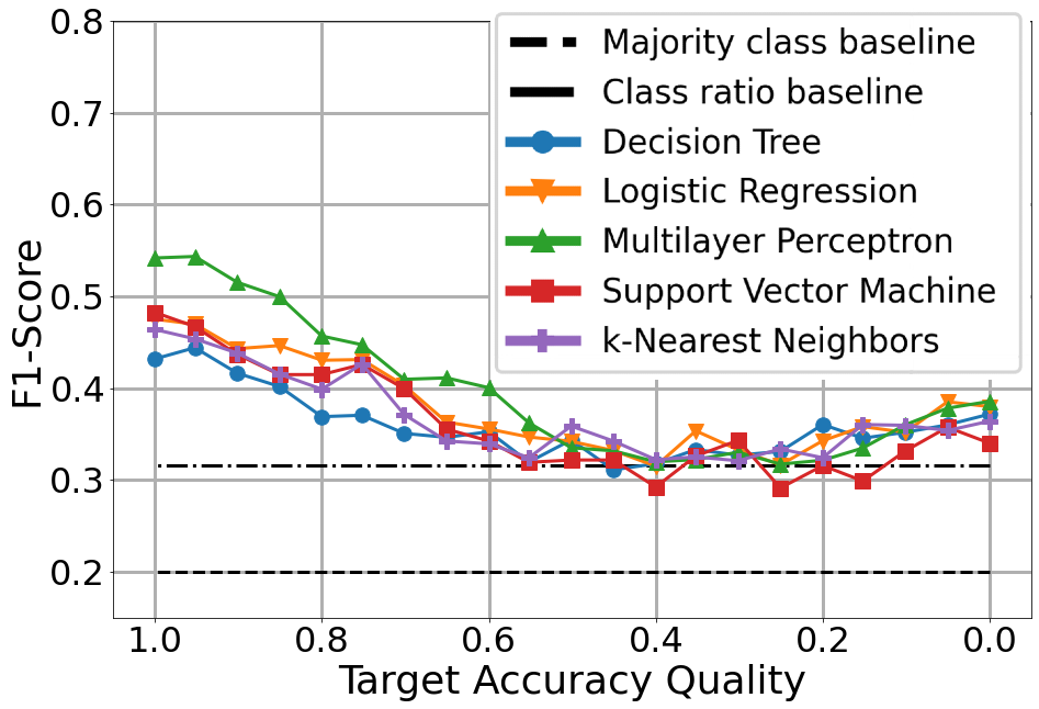
For Scenario 3 (Figure 8 third row), we observed a similar behavior of the algorithms as in Scenario 1, with one major difference: After polluting 1 divided by the number of classes of the samples both in the training and testing data, the score starts to increase at different slops for all algorithms regardless of the dataset.
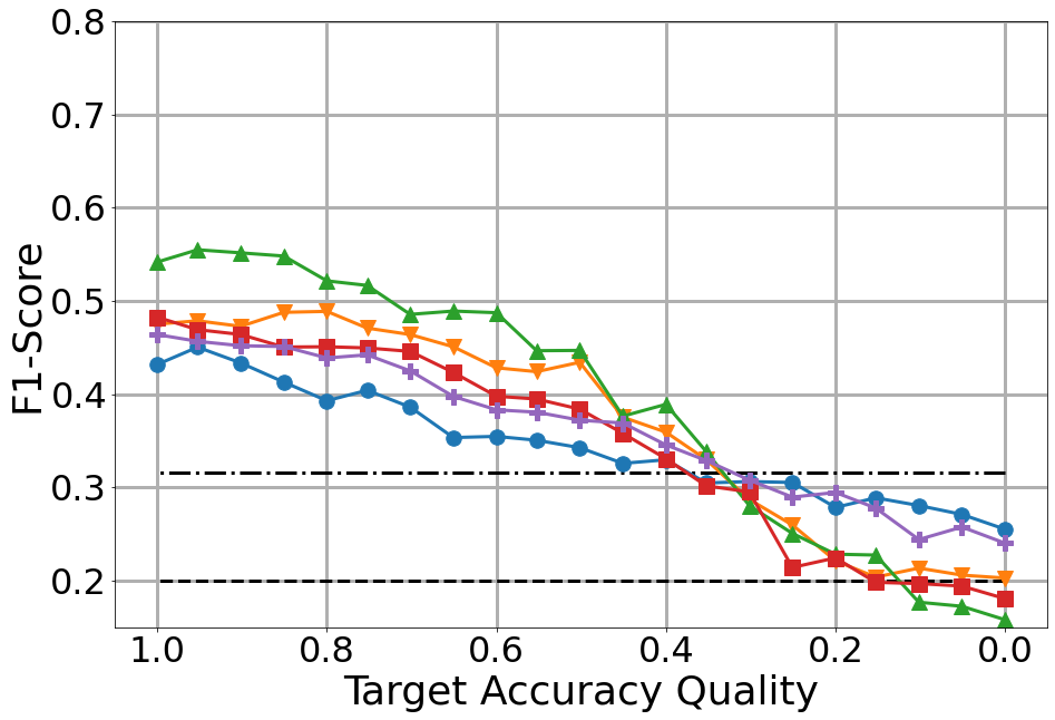
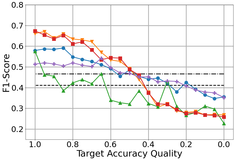
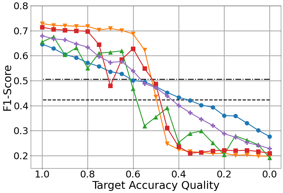
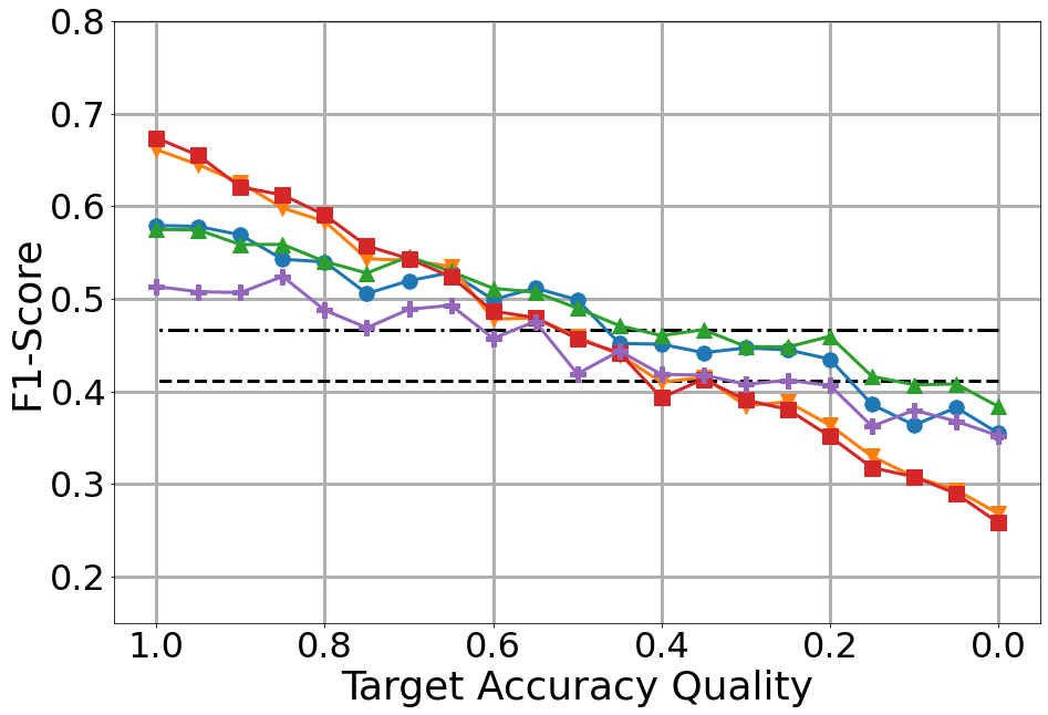
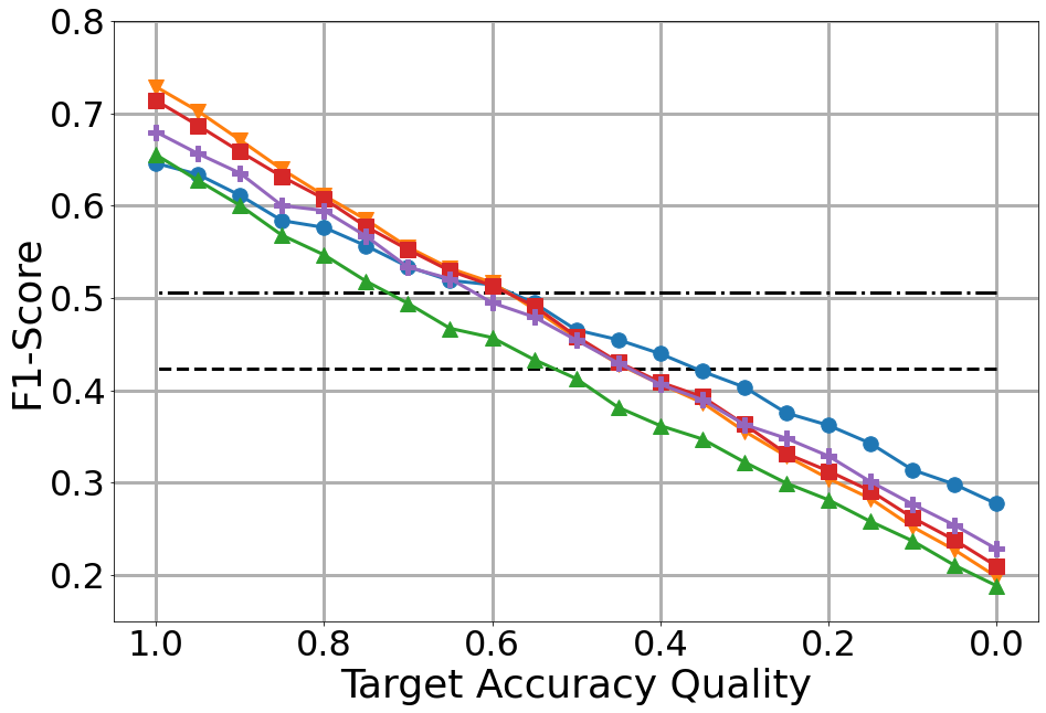
The second scenario in the second row in Figure 8 shows a situation where the training data was labeled cautiously, but the test data contains mislabeled samples. The results of Scenario 2 can be interpreted as the margin by which the performance is underestimated w.r.t. to the actual performance in clean data. This also follows a linear trend and is consistent across all datasets, with only slight differences in the slopes of the linear trend. Twenty percent more incorrectly labeled samples in the test set leads to an underestimation of up to about 10%, which shows that labeling the test set carefully is crucial. If the test set has many mislabeled samples, then this could result in scrapping the model as it performs below the baseline even though it is much better in reality (see the cross-section of model performances and baselines, e.g., in Figure 7(f)).
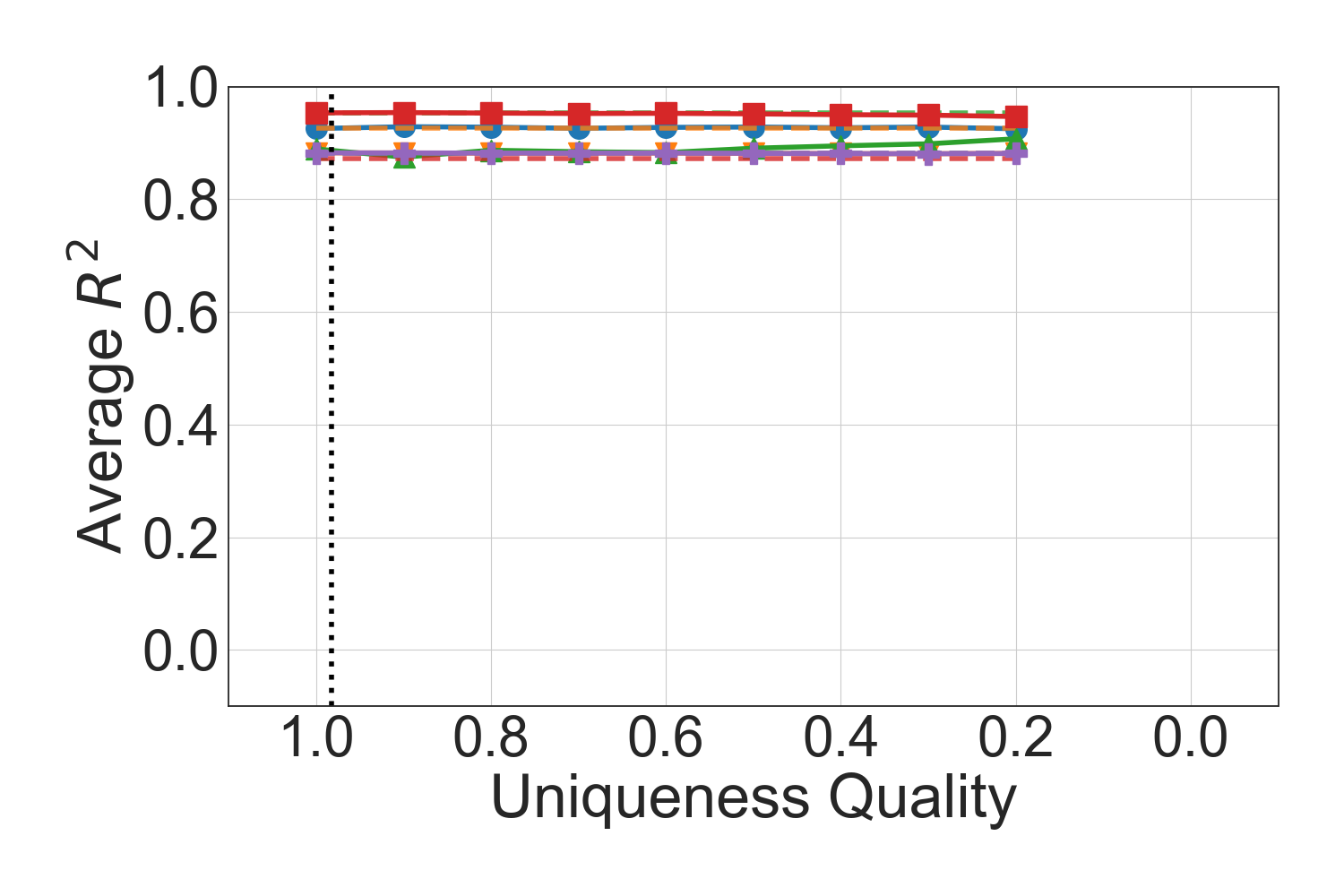
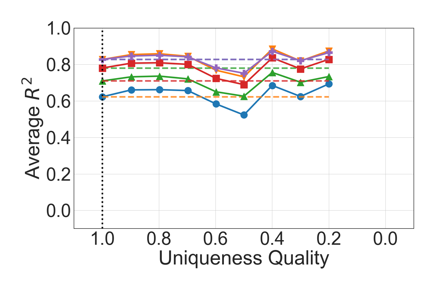
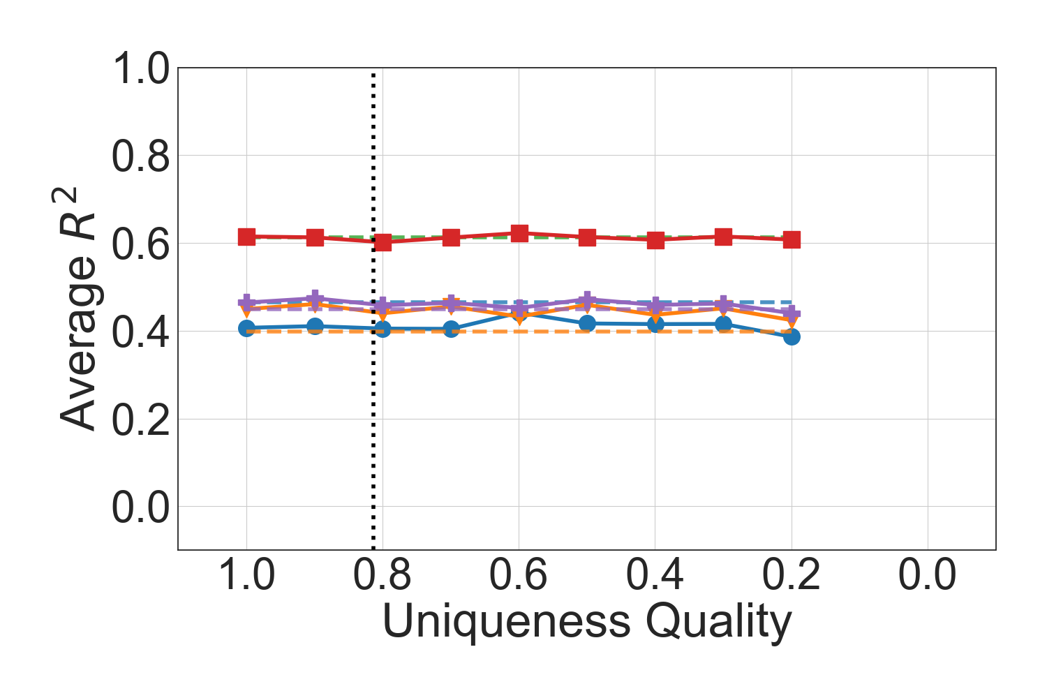
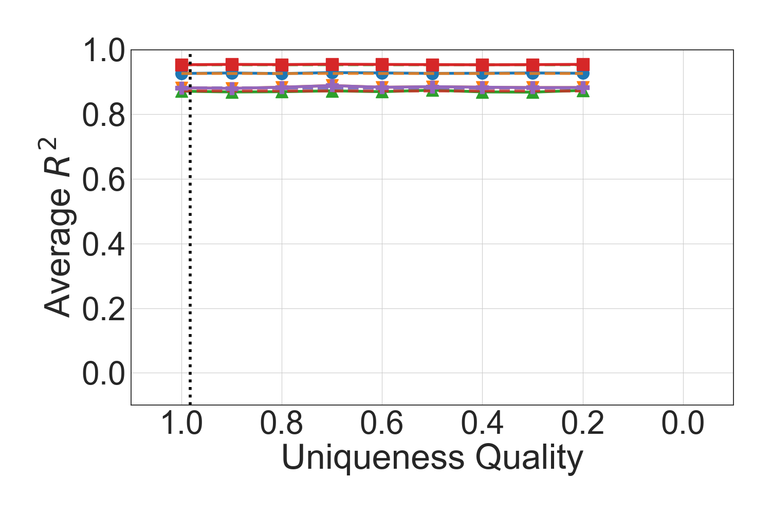
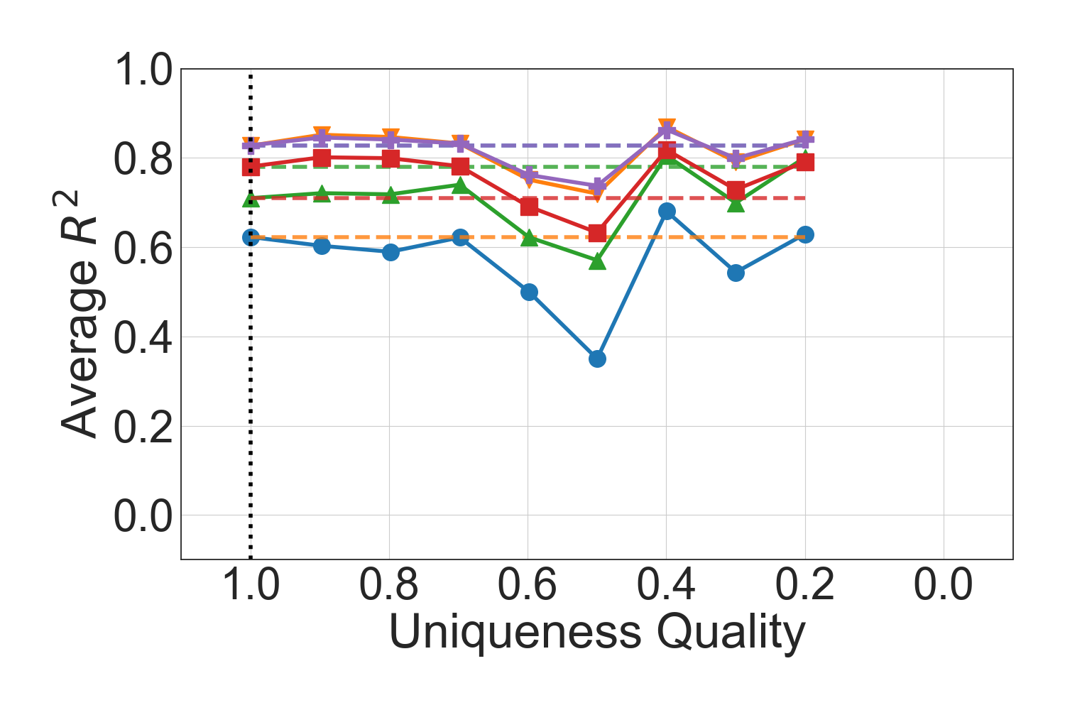
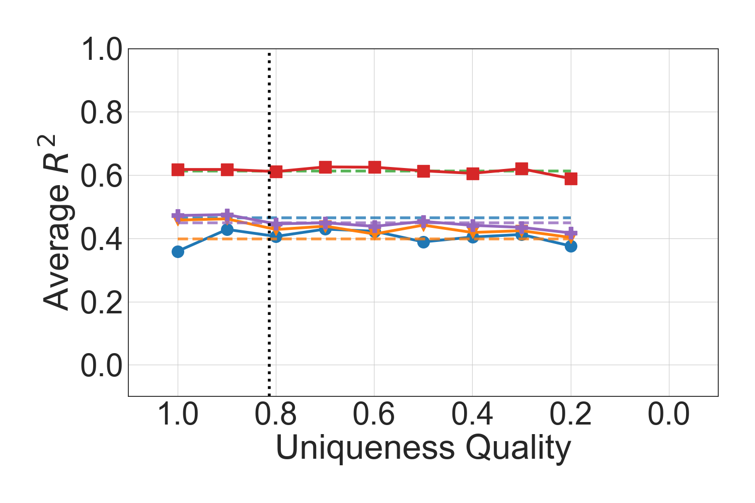
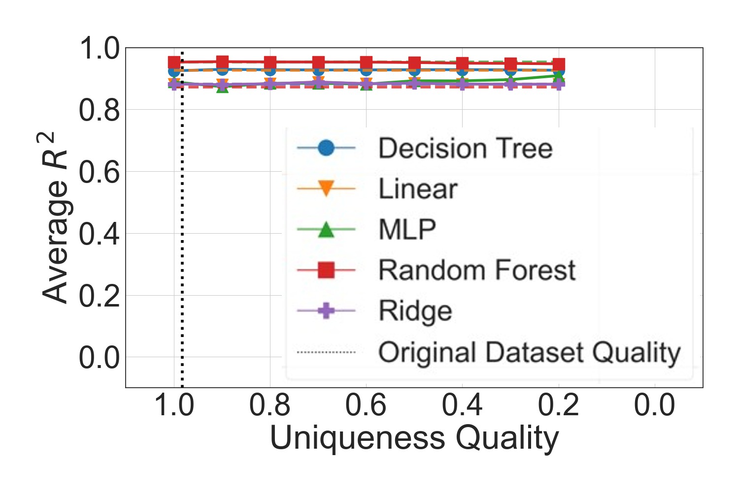
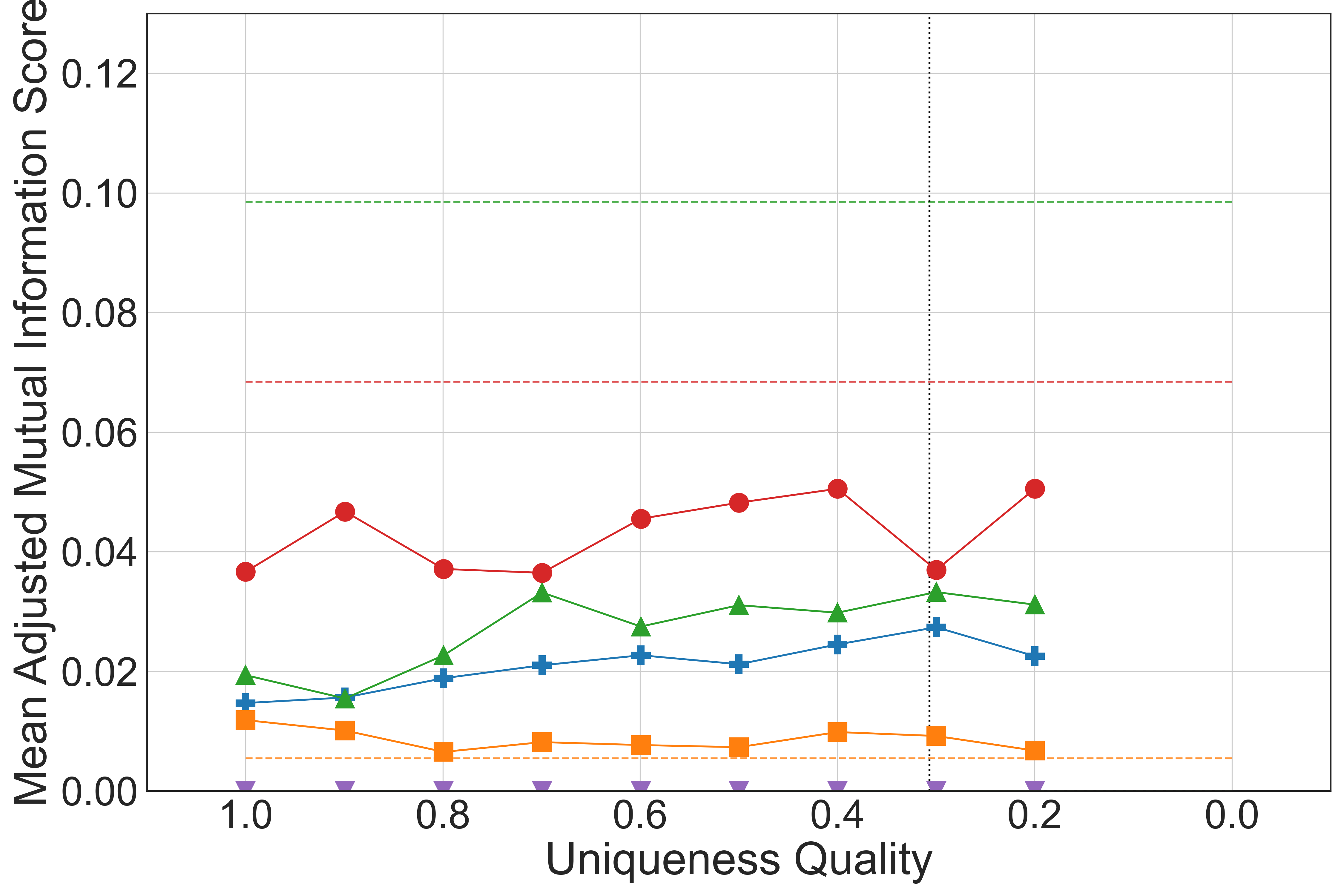
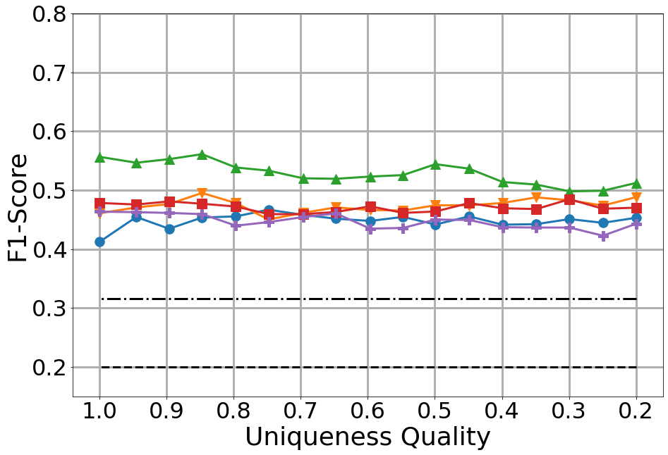
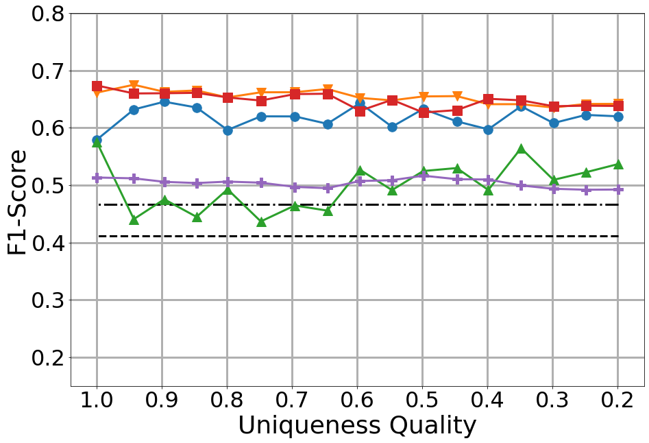
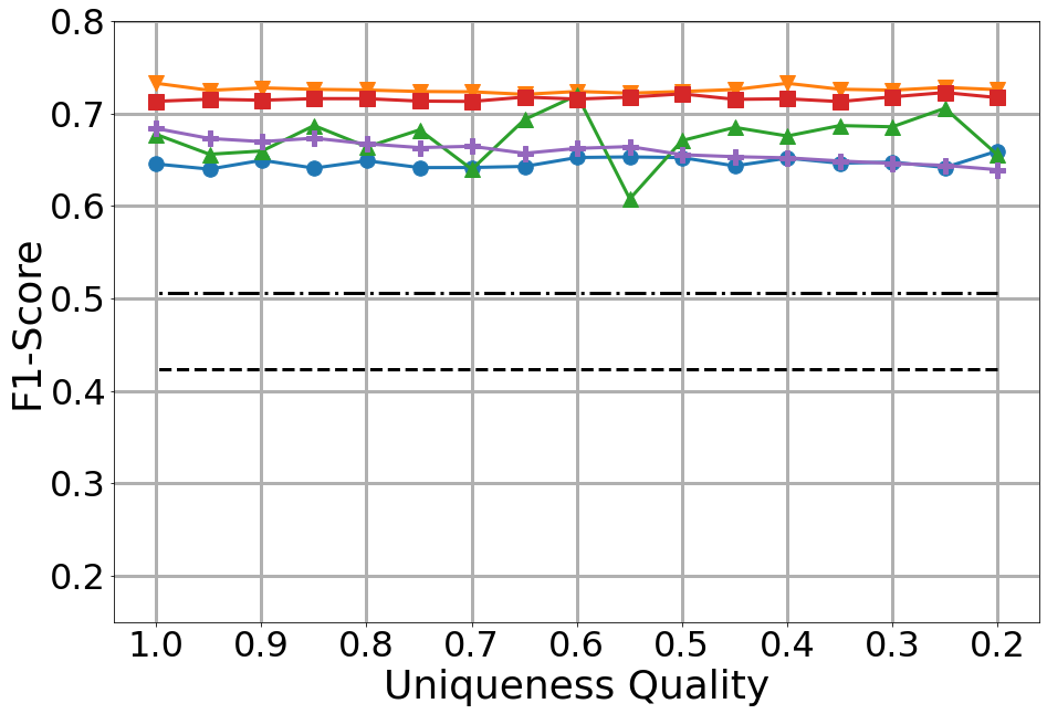
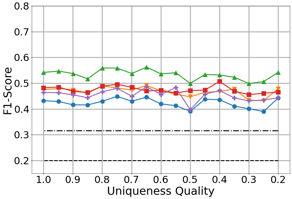
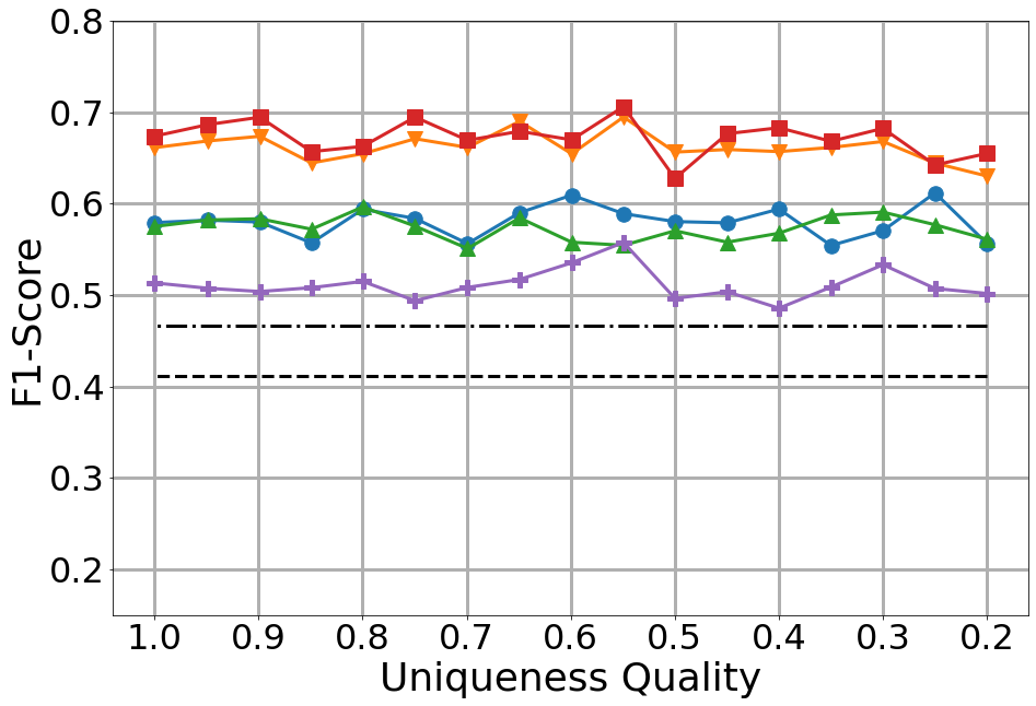
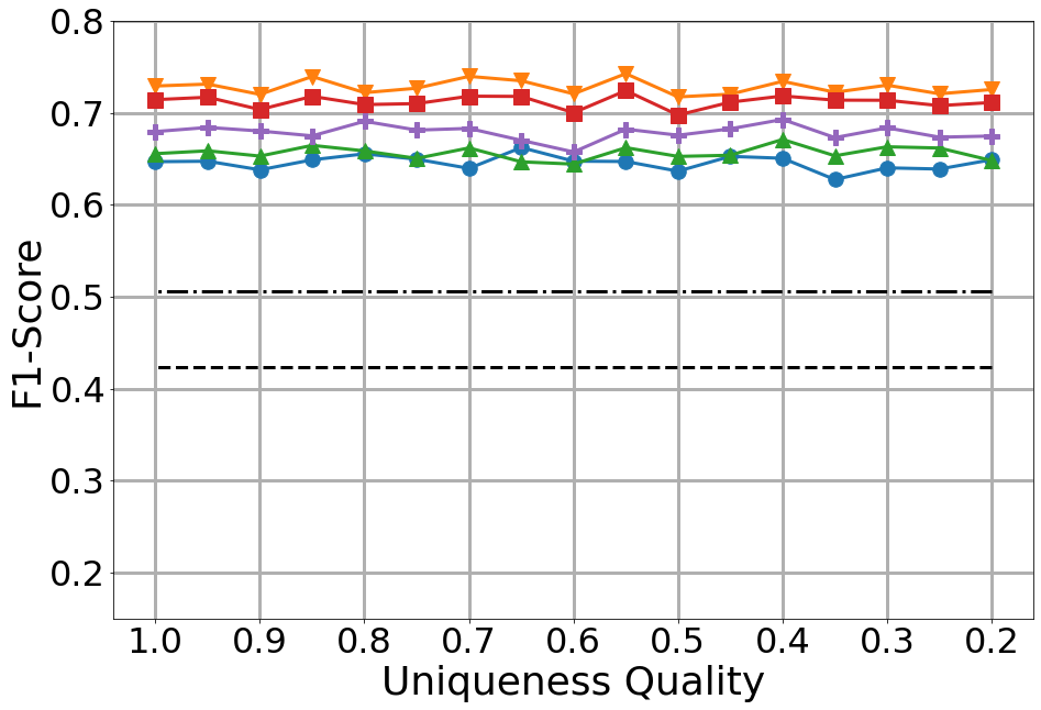
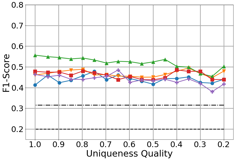
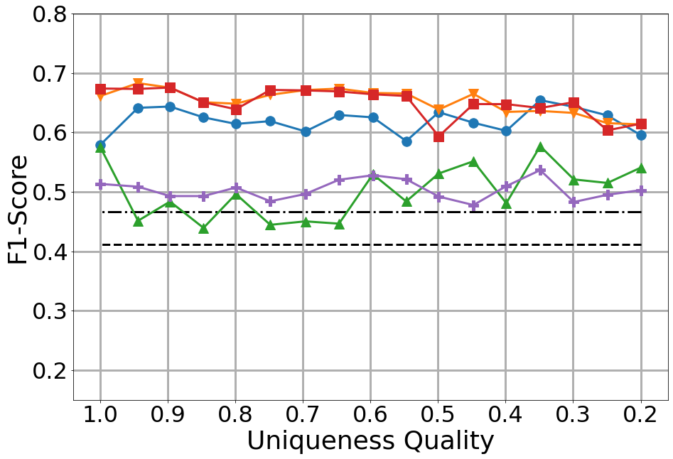
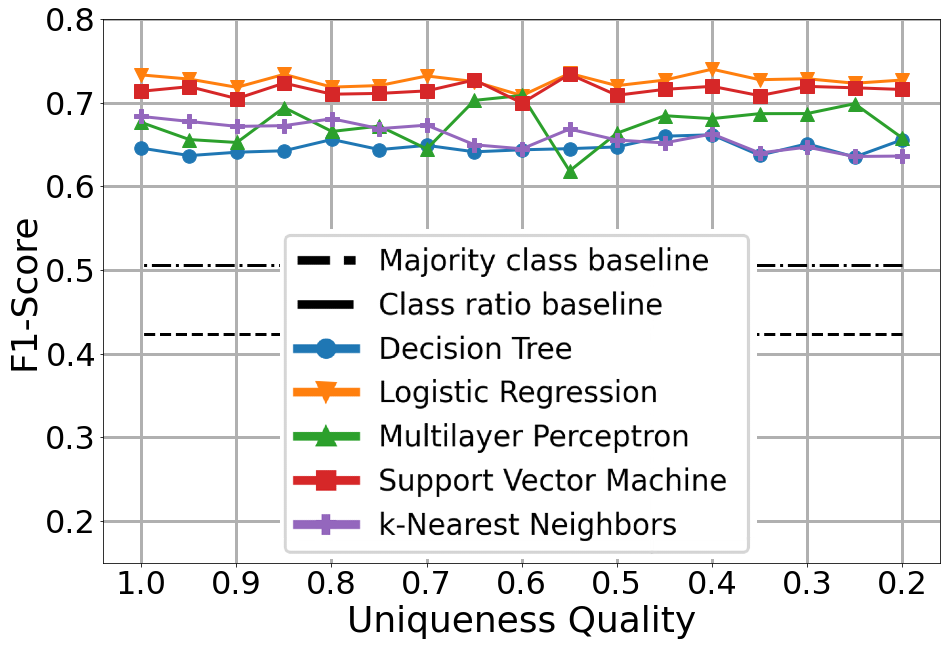
Uniqueness.
For all datasets, uniqueness does not have much of an impact on the performance of all classifiers in all scenarios, as can be seen in Figures 9. The largest drop in is observed for DT and MLP on Credit. This drastic drop in performance is attributed to the size of Credit, only 1 000 records, where generalization is already difficult enough, so introducing duplicates gives too much weight to single instances. On the one hand, it is interesting that MLP performance already drops with 5% pollution in Scenarios 1 and 3 on Credit (Figures 8(b) and 8(h)). This suggests that de-duplication is an important pre-processing step before training an MLP on a small dataset. On the other hand, the results on the other datasets with linear models suggest that exact duplicates in both training and testing data do not significantly decrease classification performance.
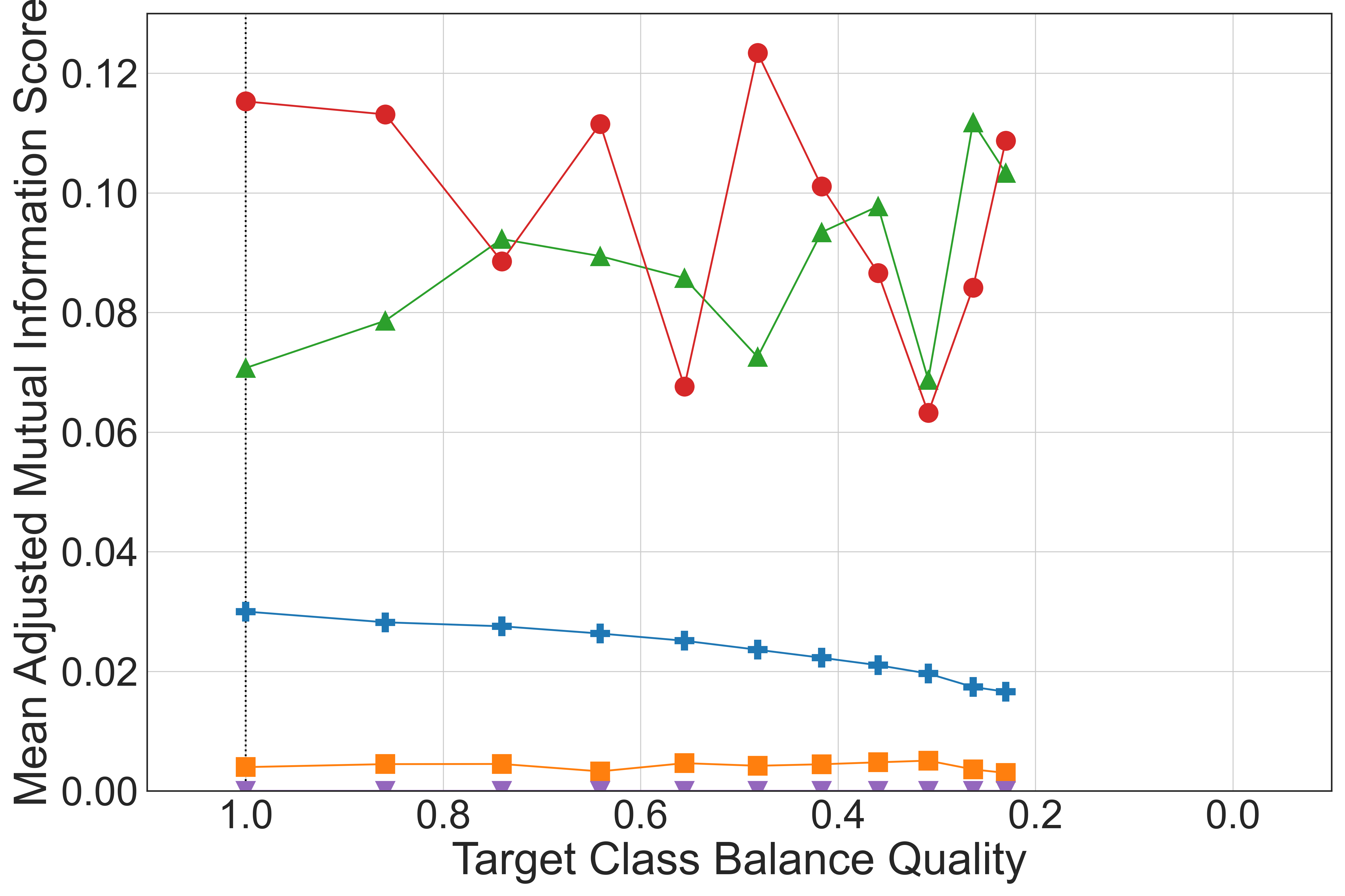
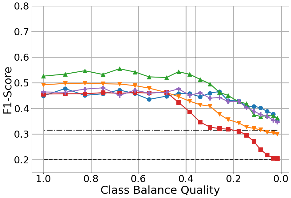
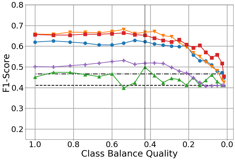
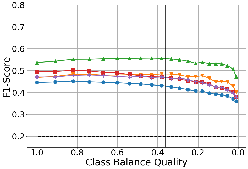
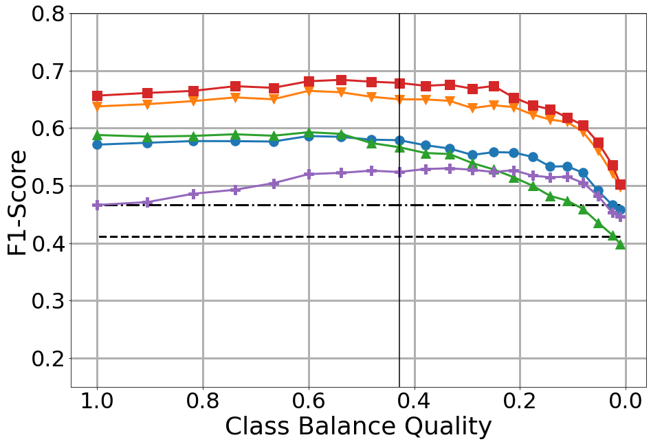
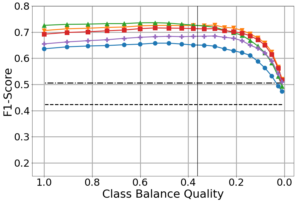
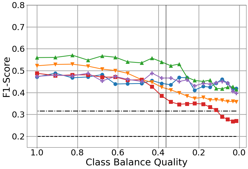
Target Class Balance.
As mentioned before, every target class balance plot has an additional vertical line, which indicates the target class balance quality of the original dataset. In Figure 10, we start by training on a balanced dataset (quality of 1.0) and as the quality decreases the imbalance of the target variable increases towards the original majority class. It is important to mention again that the imbalance shifts towards the original majority class, as this explains the gain in performance for most of the algorithms up to a certain point (e.g., a quality of about 0.25 in Figure 9(c)). In Scenarios 1 and 3 (first and last rows in Figure 10), once the imbalance affects more than half the samples for the binary classification datasets, all algorithms’ performance slowly drops towards the performance of the majority class baseline, because they are trained on only a handful of samples from the minority class and therefore have no chance to actually learning the patterns of this class. All the algorithms behave similarly until this point, with only a few exceptions (mainly SVM and MLP). This suggests that the training data does not have to reflect the actual real-world class balance, as long as it is equally or more balanced. The robustness to training on data that is more imbalanced than the testing data (to the right of the vertical line) is more dataset-specific. For example, we can see in Figures 9(b) and 9(h) that the performance drop on Credit is less drastic and takes longer to manifest itself than for the other datasets.
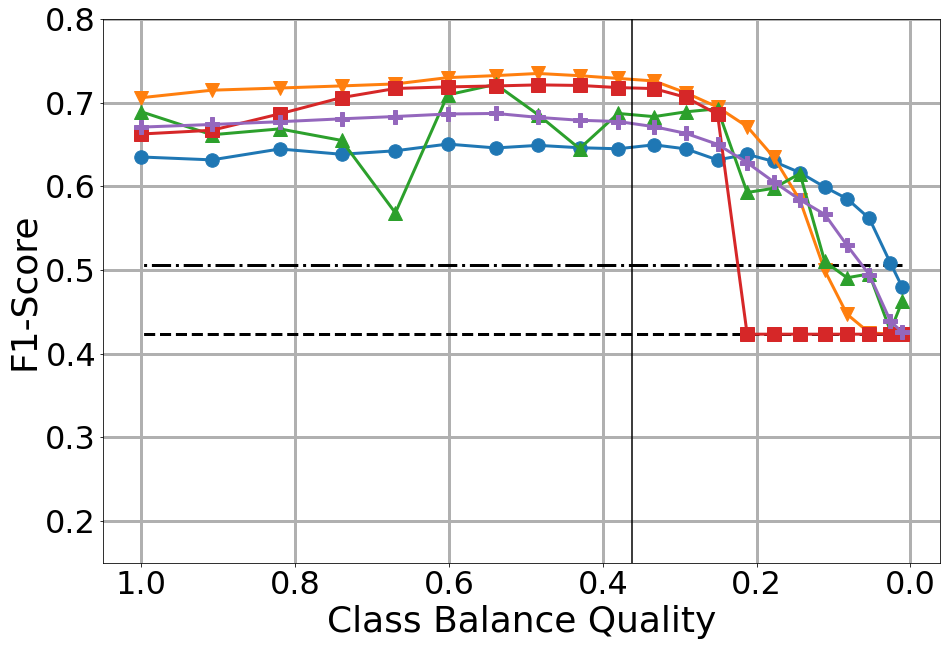
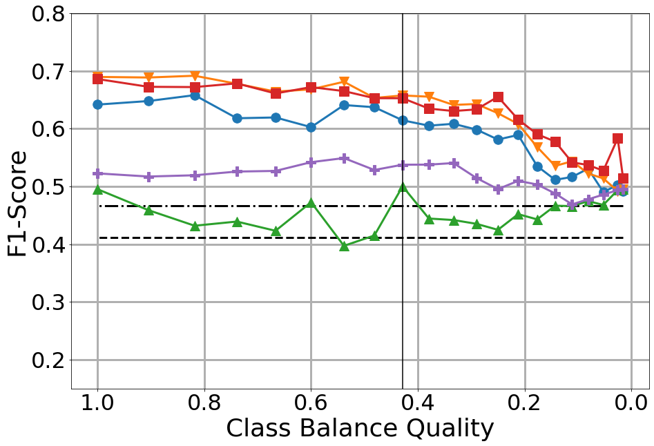
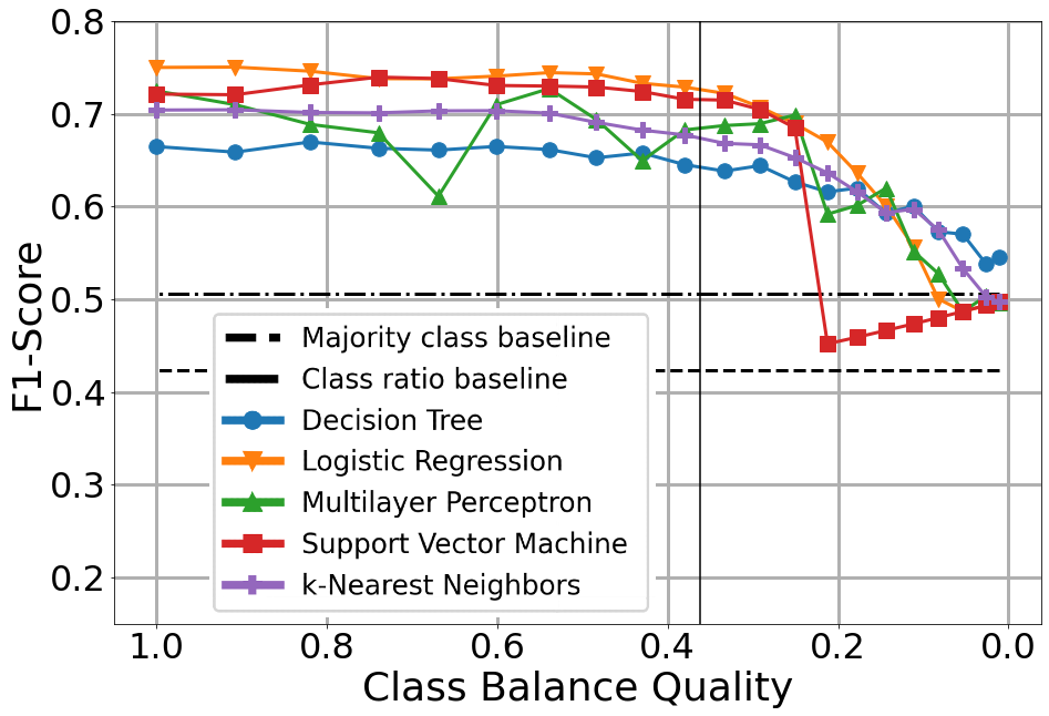
For Scenario 2 (the second row in Figure 10), which reflects the real-world situation of training a model on an initial batch of real-world data and once the model reaches production, there is a distribution shift in the serving data that enters the pipeline. we observe that the models are very robust against the distribution shift, which moves towards a balance in class frequency, and they sometimes even increase their performance (only the KNN in Figure 9(e) worsens significantly). Just like in Scenario 1, the performance on class imbalance past the original class balance is dataset-dependent and for example much steeper for Telco than for the other two datasets as we see in Figure 9(f).
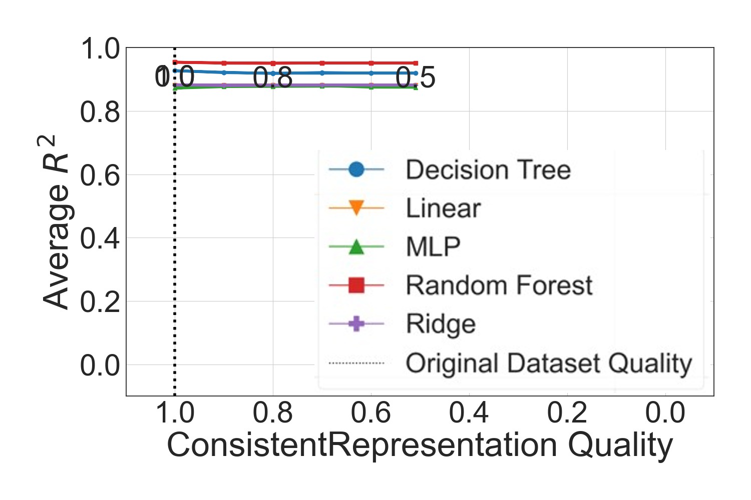
6.2 Regression
We discuss here the effect of degrading the six data quality dimensions of three datasets, namely: Houses, IMDB and Cars on the performance of five regression algorithms, namely: LR, RR, DT, RF and MLP. As LR and RR differ only in the regularization employed in RR, their performance lines in the result plots often overlap. This means that in cases where the LR performance line is not visible at all in a plot, it is hidden behind the RR line. We only show of or larger, since a negative means that the model is worse than always predicting the mean. Thus, a model in the negative ranges would not be of interest and the resulting vertical axis scale would make it harder to analyze the behavior in the range of interest, to . As the MLP performance on IMDB is already negative without pollution, the MLP line is not visible in the plots for IMDB.
Consistent Representation.
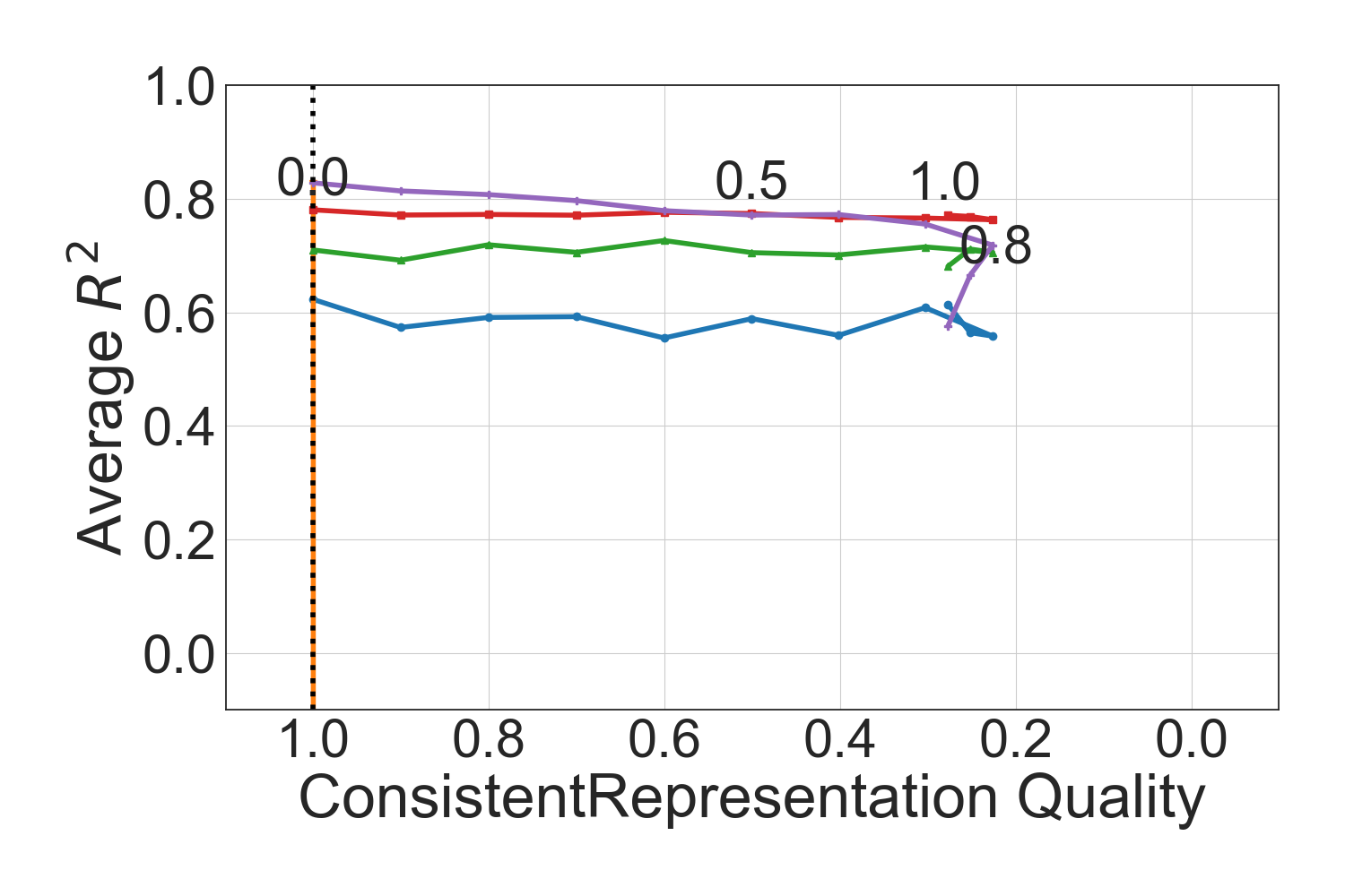
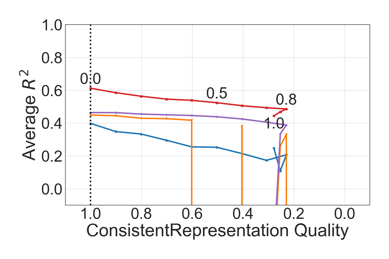
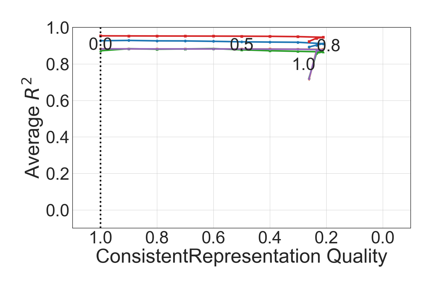
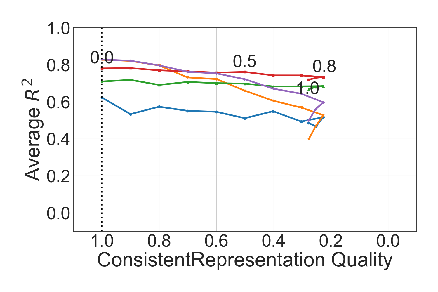
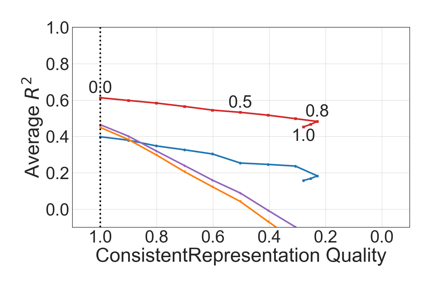
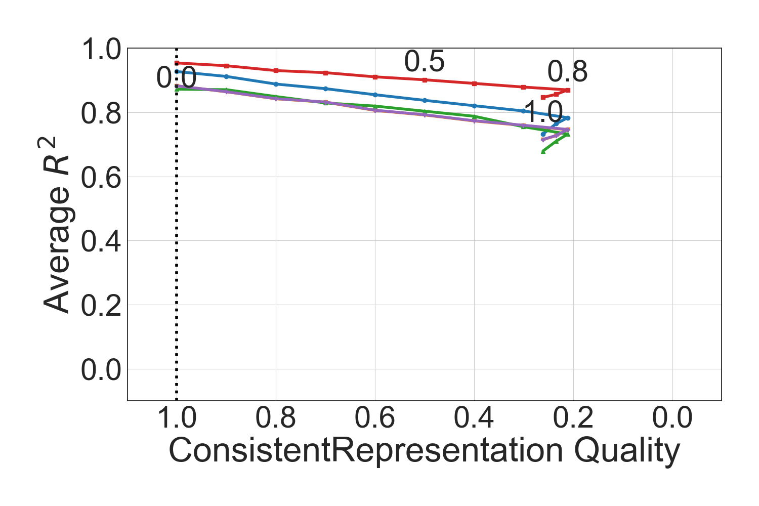
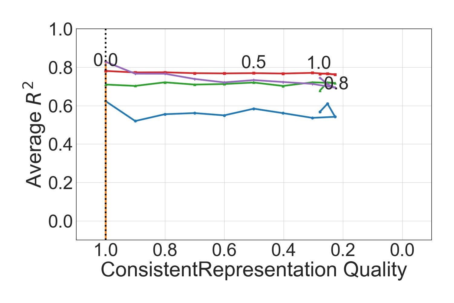
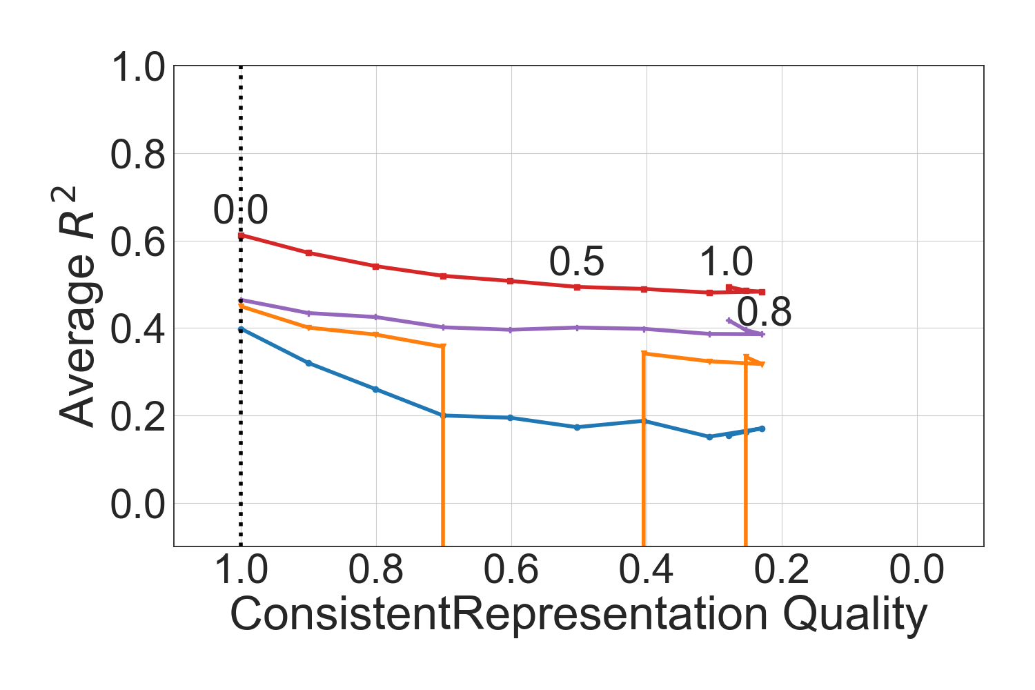
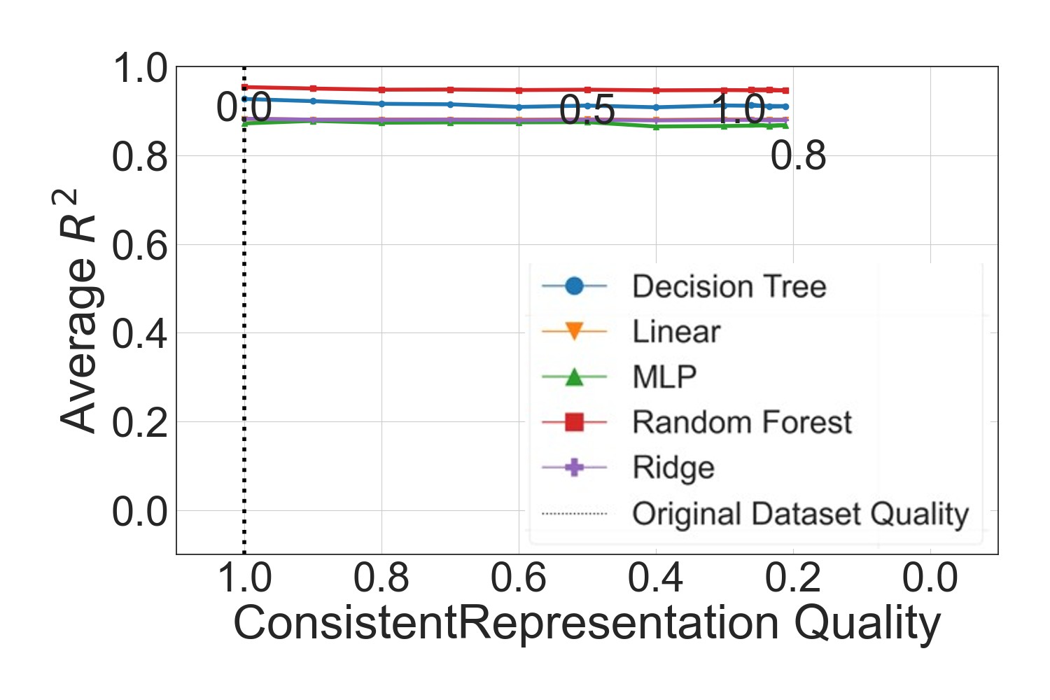
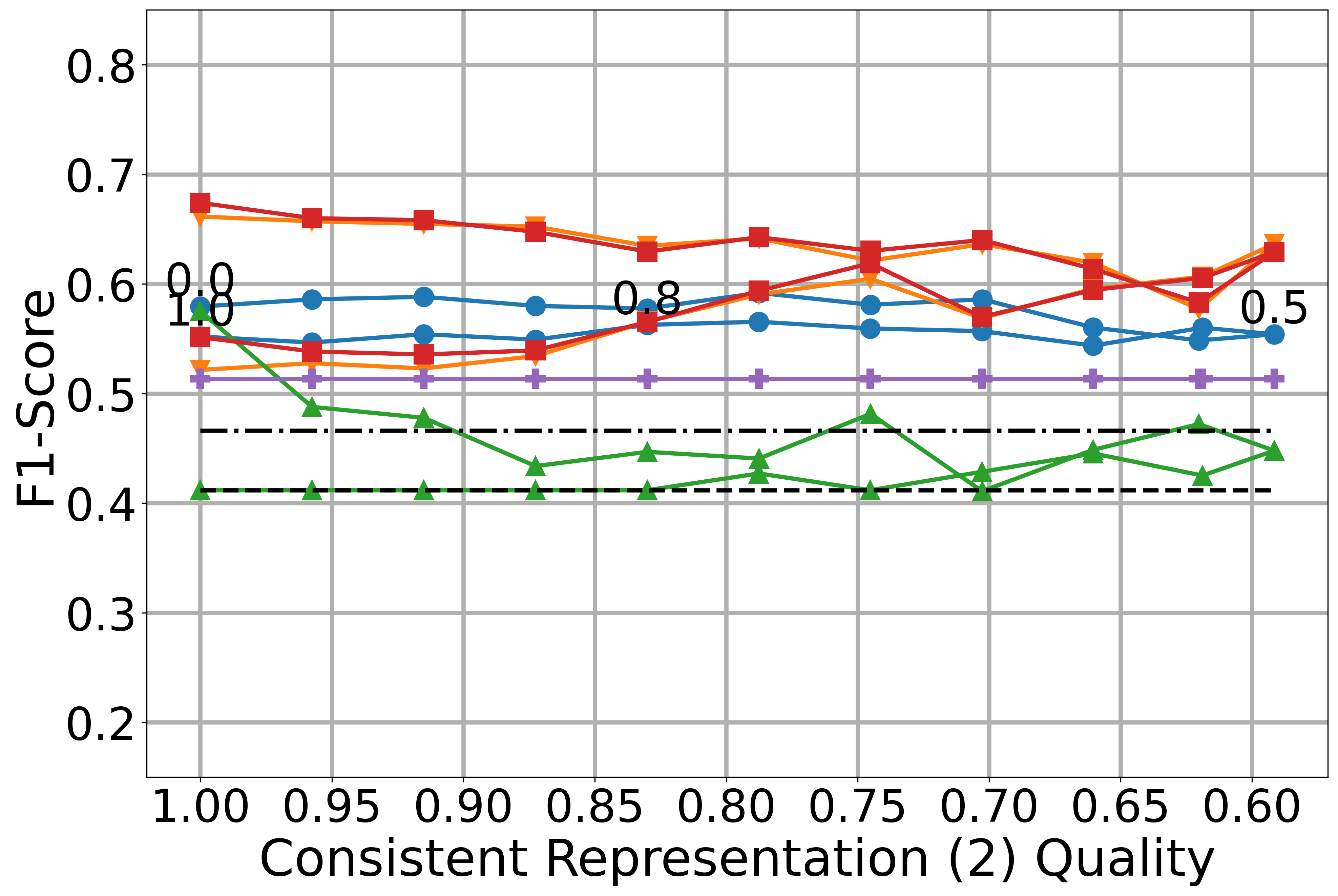
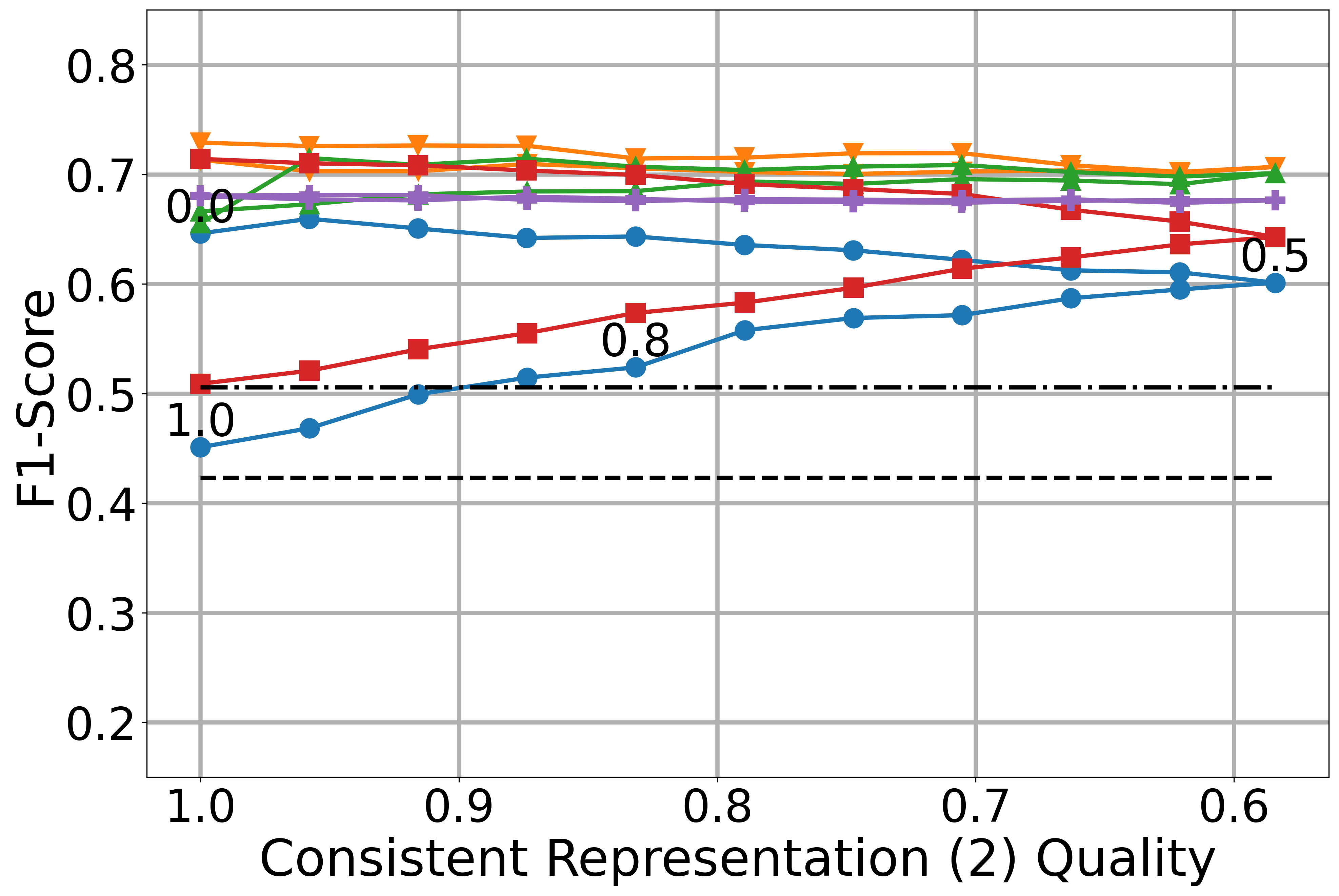
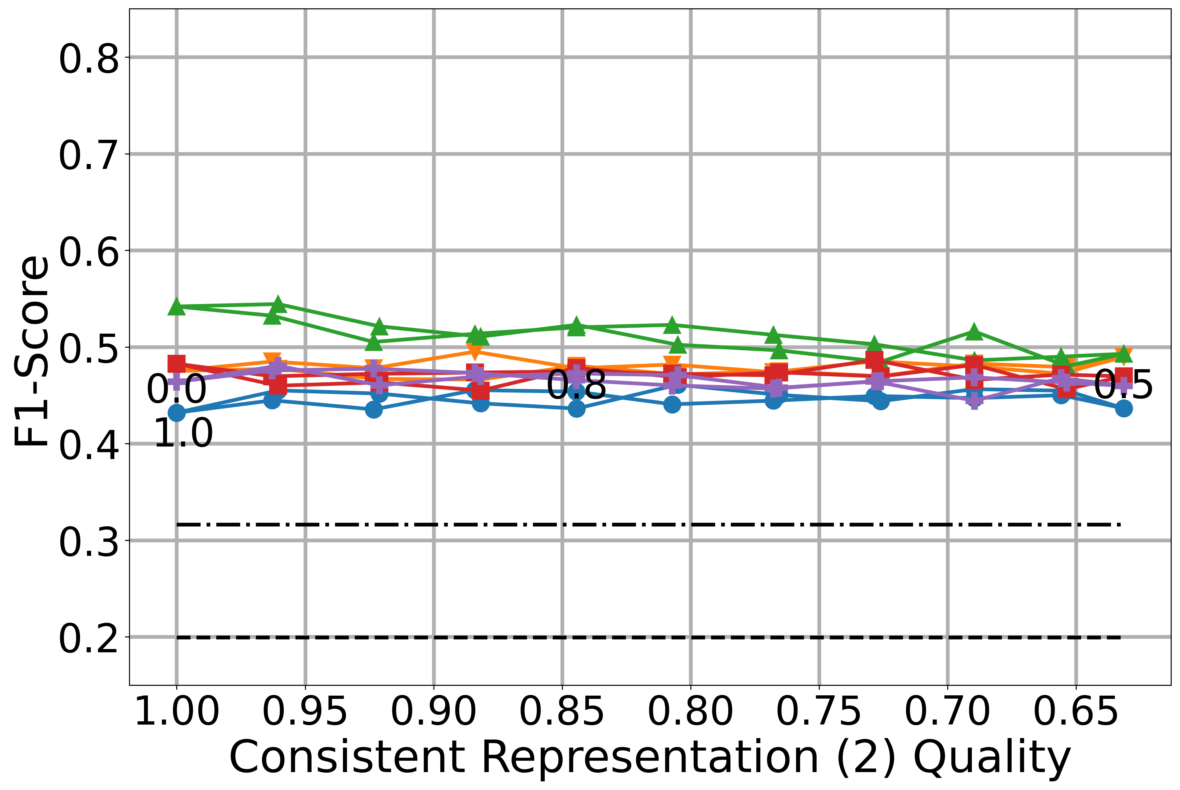
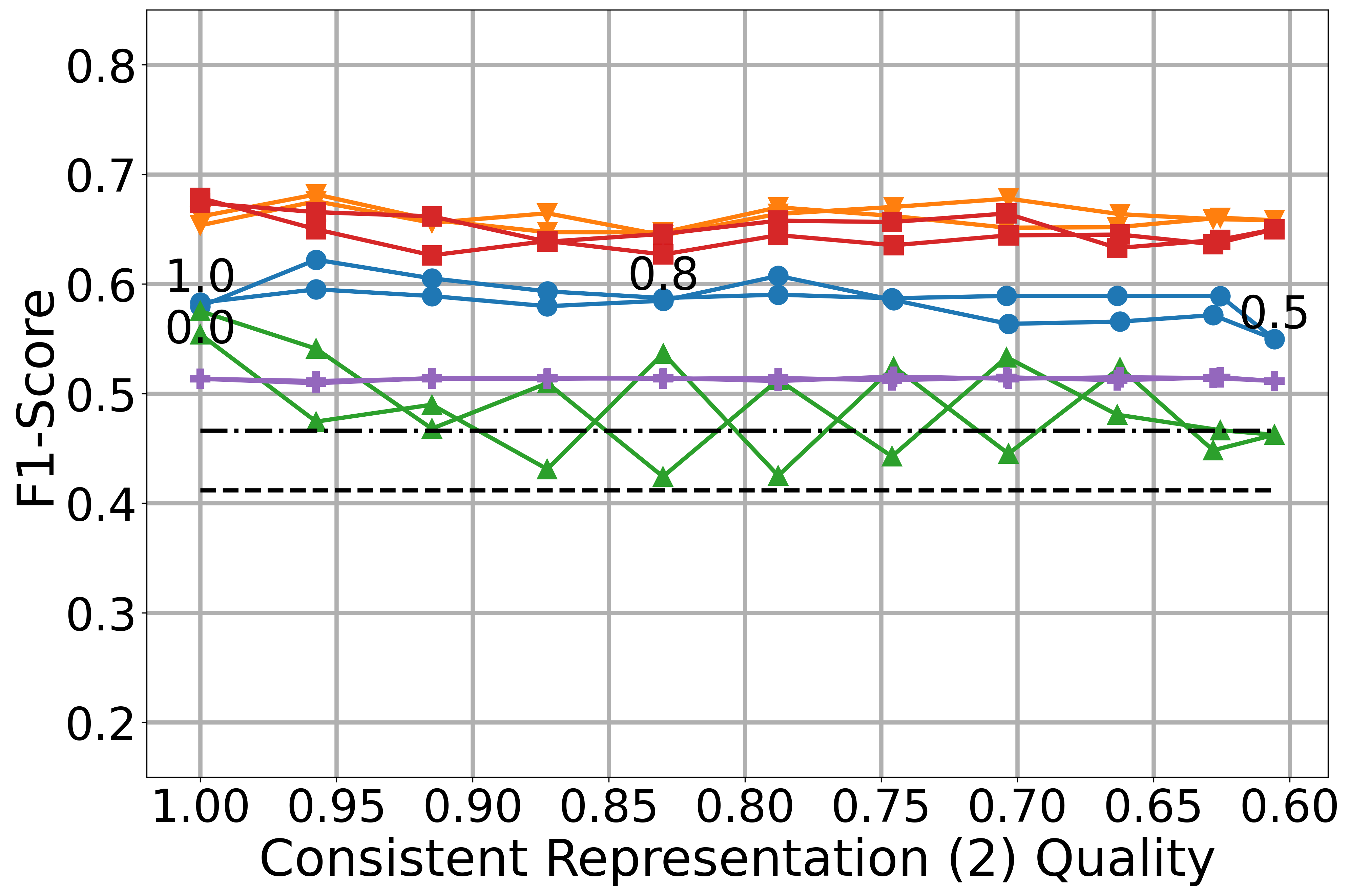
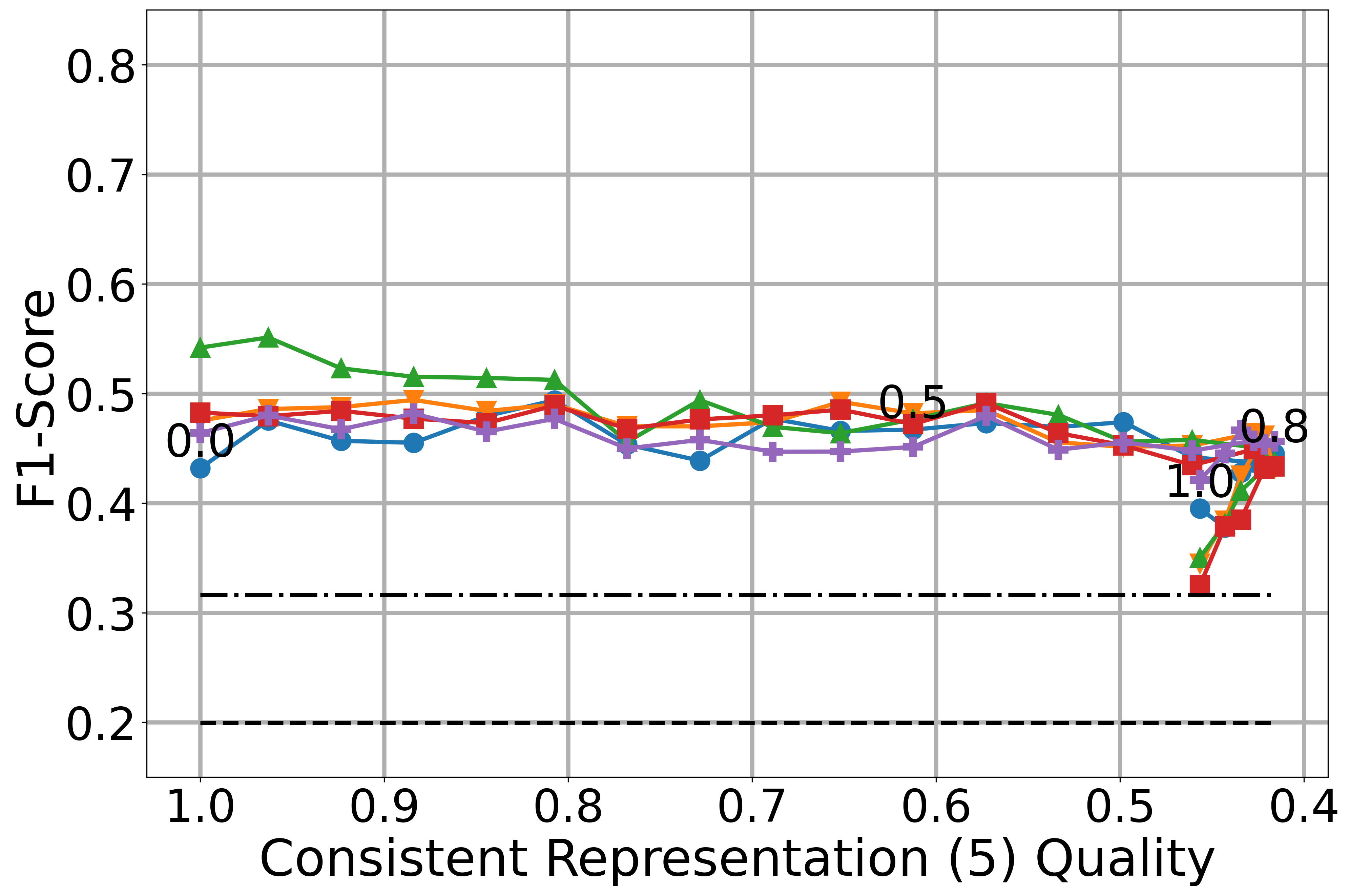
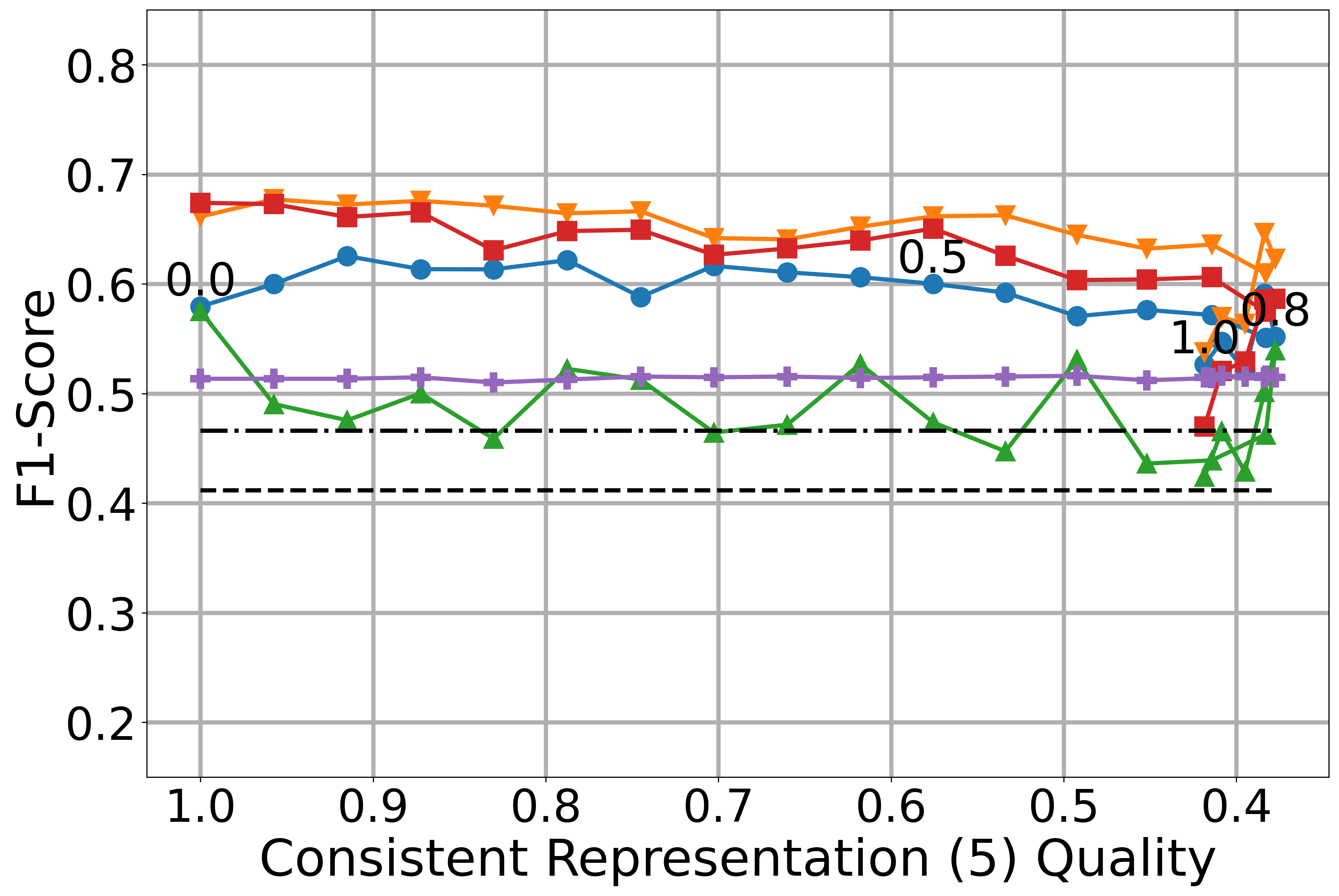
For consistent representation, we show only a plot with adding 4 new representations per unique value, i.e., . The plots for can be found in Figure 24 in the Appendix. As described in the introduction of Section 6, a higher percentage of polluted samples can lead to an increase in quality again, which is why lines go backwards when more than of samples are polluted for . We add some percentages next to the lines for better orientation. An increase of the representations of values in categorical features leads to a decrease in of all algorithms, as shown in Figure 11. The severity of this decrease depends on the scenario. In Scenario 2 (second row in Figure 11), when the inserted inconsistent representations have not been present during training, the performance decrease is the largest, especially for RR. In the two other scenarios, LR performance drops drastically, even for small percentages of pollution.
Adding inconsistent representations during training but not during testing, i.e., Scenario 1 (first row in Figure 11) has a smaller effect, except for LR, with the fastest performance drop mostly at a percentage of polluted samples of more than . The effect of the pollution is smallest in Scenario 3 for Houses (Figure 10(g)) and Cars (Figure 10(i)),and for IMDB (Figure 10(h))it is more similar to Scenario 1 (Figure 10(b)). We observed for Scenario 3 a sudden increase in of most algorithms when the percentage of polluted samples is larger than , which is not surprising as the new representations are added in both training and test set. However, with 4 new representations per value, this does not happen for all datasets and algorithms, as there might still be confusion for the algorithms in some cases. Looking at the algorithms, LR often shows considerable outliers when the training set is polluted. Due to the one-hot encoding of categorical features and LR learning a linear impact of each of those one-hot features, LR is affected by the inherently discrete differences in the one-hot features. The regularization of RR fixes this extreme behavior. LR and RR both show a larger performance drop than the three other algorithms in Scenario 2, probably due to the linear method poorly handling the one-hot features that were never during training. The tree-based methods, DT and RF, are more stable in most cases, along with MLP. The non-linearity of those methods weakens the effect of the inconsistencies in the one-hot features. The effect of inconsistency is larger on IMDB than on Houses and Cars (Figure 11). The reason for this could be the ratio between categorical and numerical attributes, which is 8:4 for IMDB and more weighted towards the numerical attributes for Houses and Cars. The observed tendencies are mostly similar when adding only one new representation during pollution, as shown in Figure 24 in the Appendix, where the quality increases again after polluting of samples. In Scenario 3, the algorithm performance rises for this increasing quality, which is expected, as the single new representation becomes the majority in both training and test set.
Completeness.
Reducing completeness of a dataset leads to a heavy performance degradation on all algorithms in all scenarios, as shown in Figure 12. The RF performance decreases the slowest, especially much slower than DT in most cases. Next comes RR, being an ensemble method makes it more robust against missing values. LR and RR show similar behavior, with RR performing better or similar than LR. The performance of MLP is mostly between that of LR/RR and DT. For all datasets, the strongest decrease happens in Scenario 2 (second row in Figure 12), where the missing values only appear in the test set, not in the training set. LR and RR are the most affected algorithms: the linear relation learned by those algorithms is easier to confuse with the newly inserted placeholders outside the features’ domain. The value that is chosen as placeholder could also have an effect, e.g., whether choosing or . Different placeholders could lead to a different behavior, which could also hold for the other scenarios and algorithms too.
The best performance is achieved in Scenario 3 (last row in Figure 12) indicating that models perform better on datasets with missing data if the missing data exists as well while the training. The effect of reducing the completeness differs per dataset. For Houses, the performance decrease in Scenario 1 is larger than for IMDB and especially than for Cars. The performance in Scenario 3 of Houses first decreases slower than in Scenario 1 and then rapidly drops when the completeness is lower than . For IMDB and Cars, the performance decrease in Scenario 3 is more of a linear form and faster than in Scenario 1. Those differences between the datasets could have their origin in the size of the datasets. For example, the small size of Houses causes the algorithms to overfit and produce better results when both training and test set contain missing values. Larger datasets could reduce this effect, making the amount of non-missing information in the test set the more important factor.
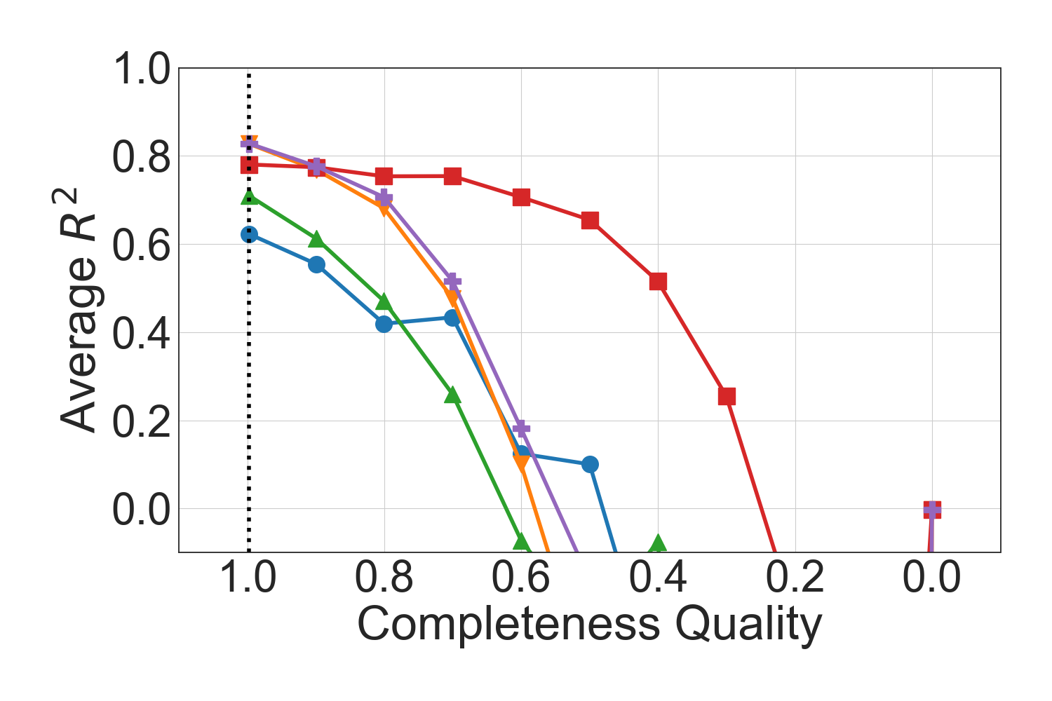
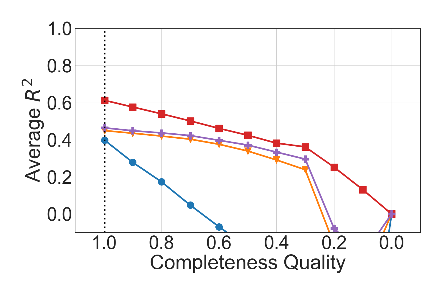
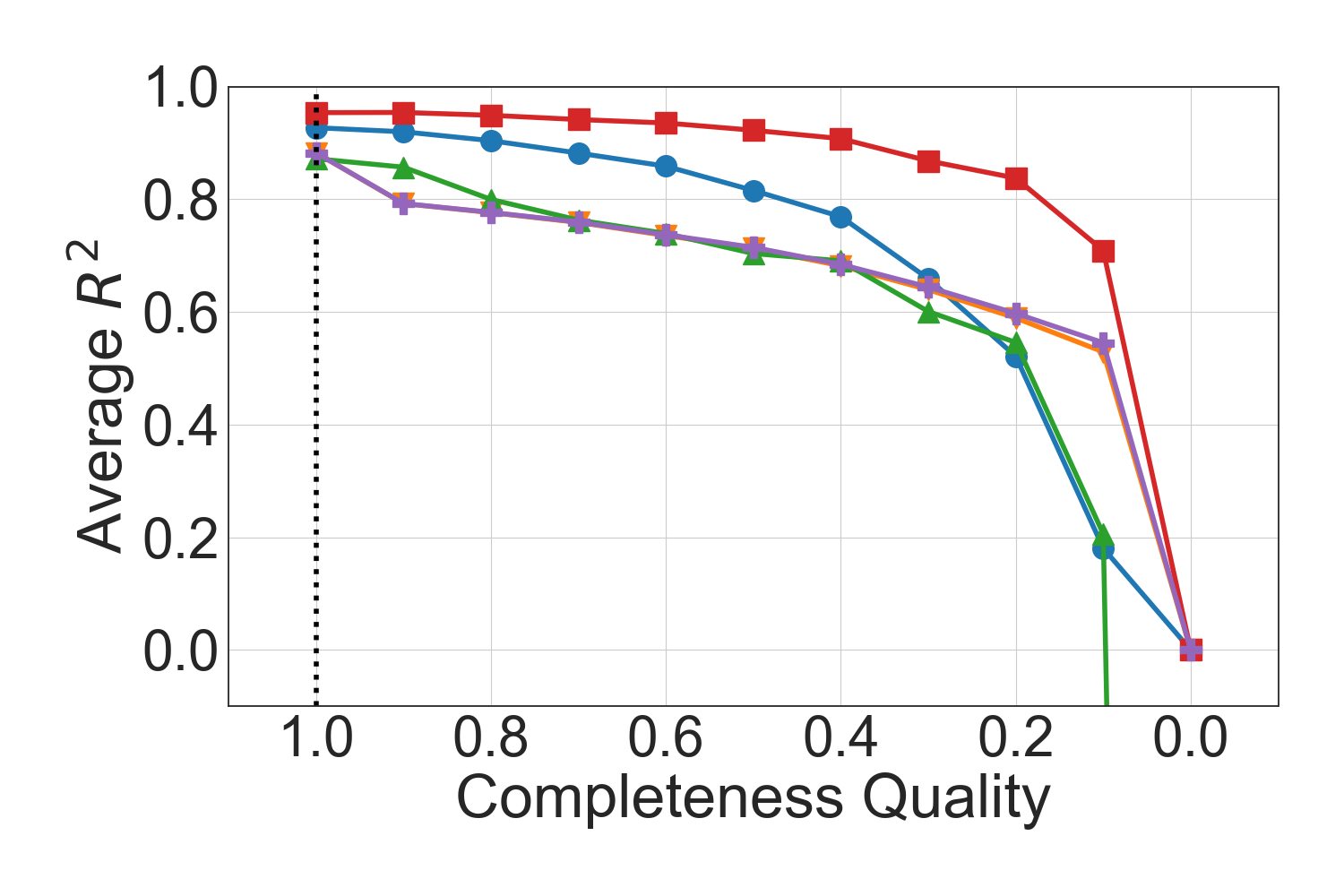
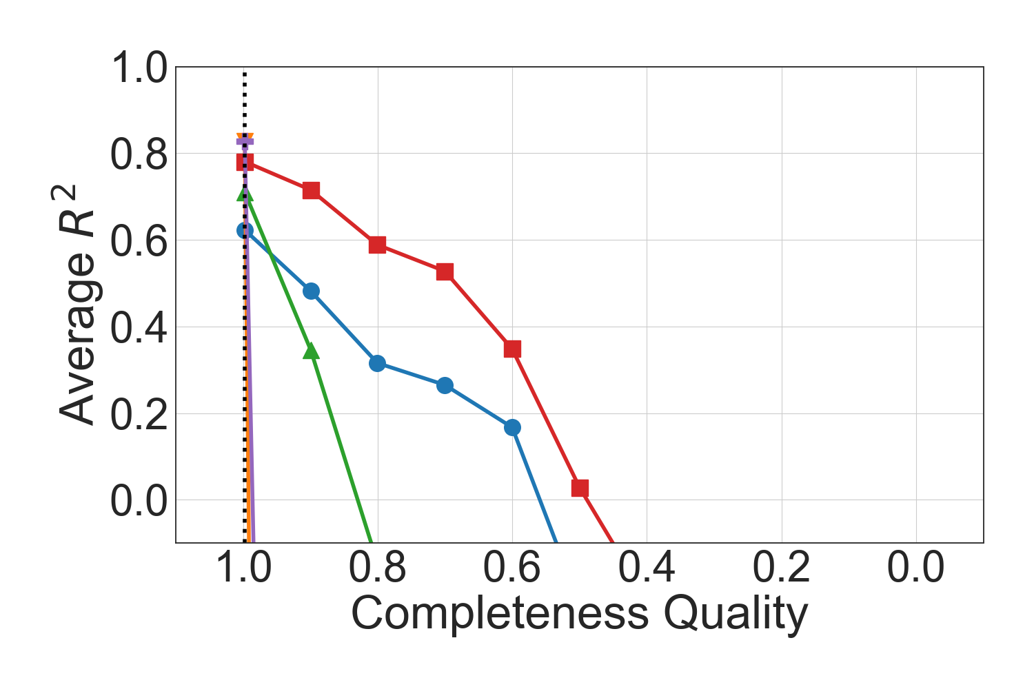
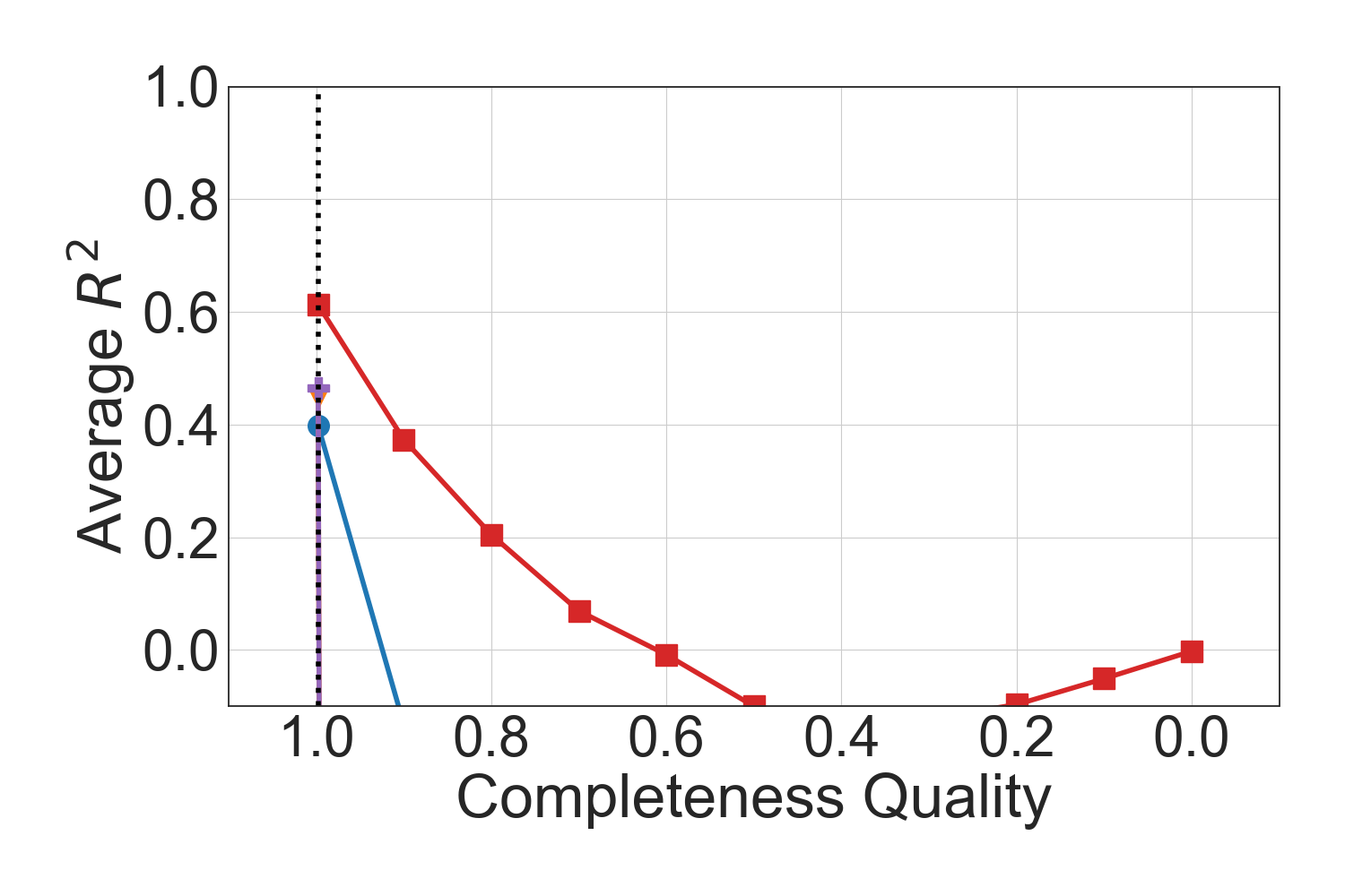
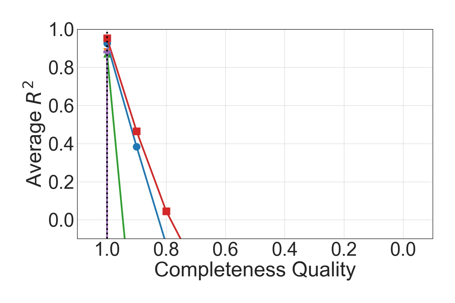
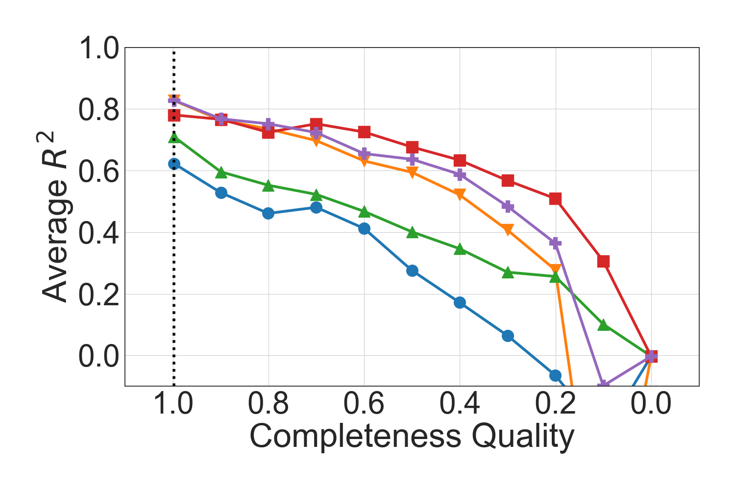
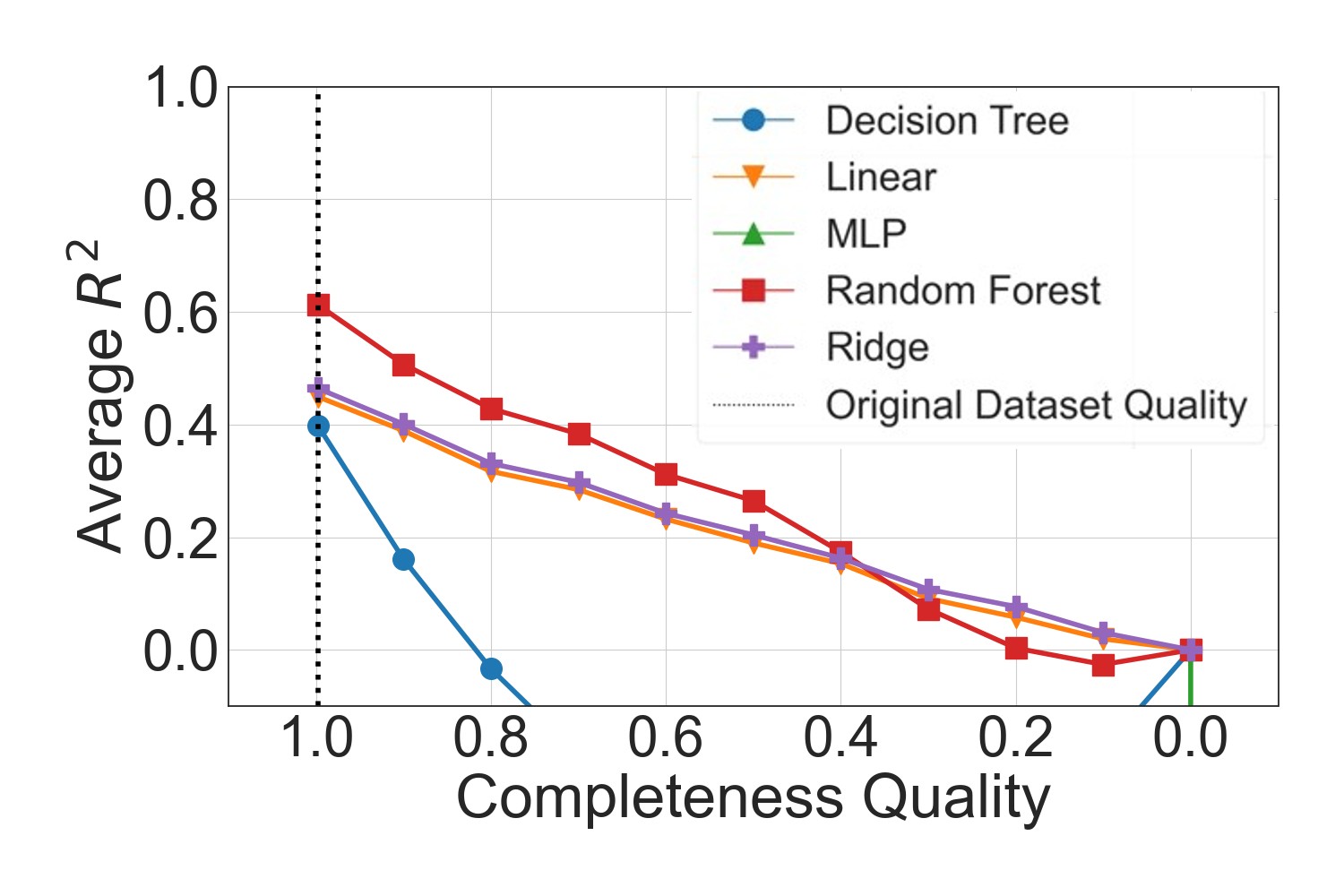
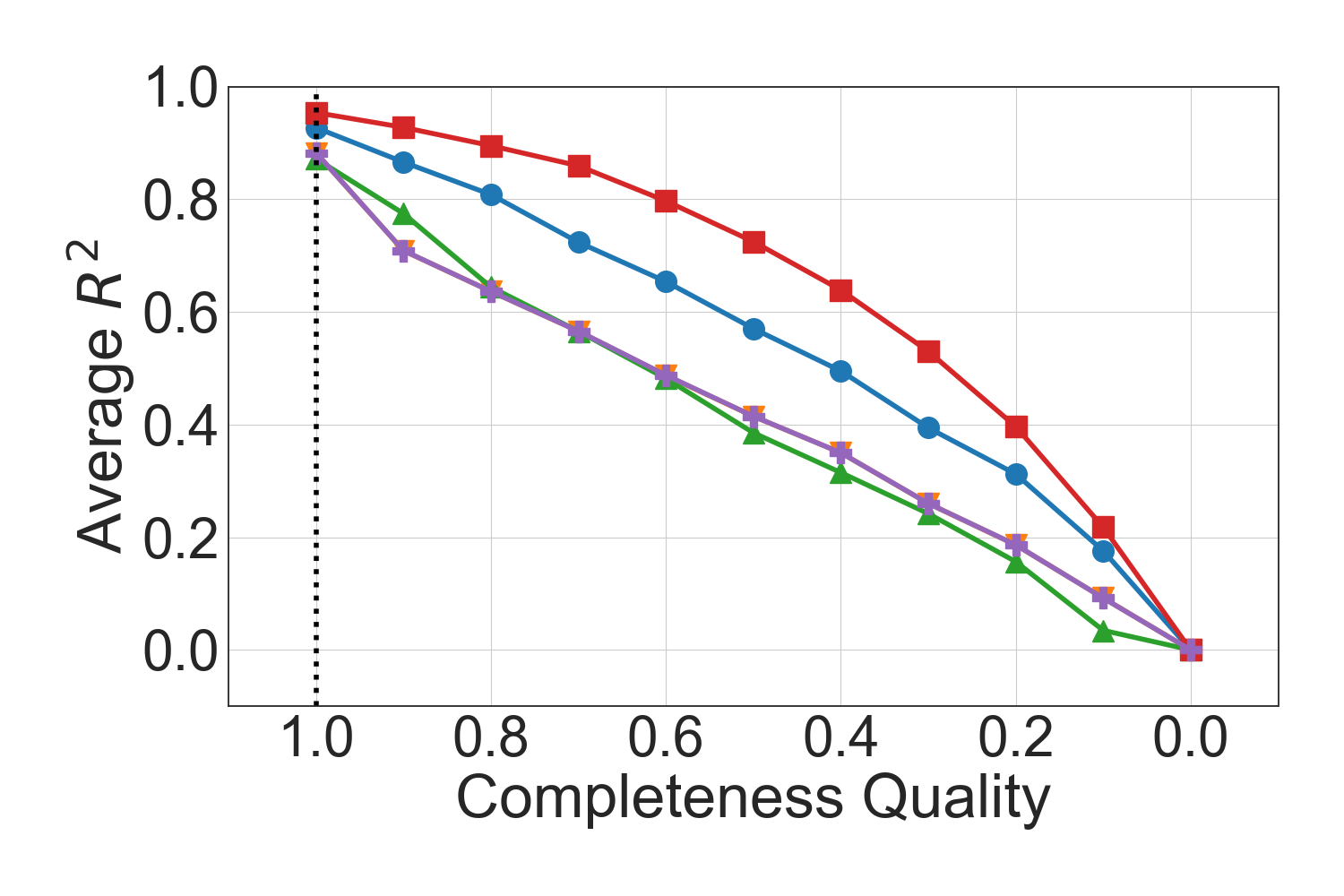
Feature Accuracy.
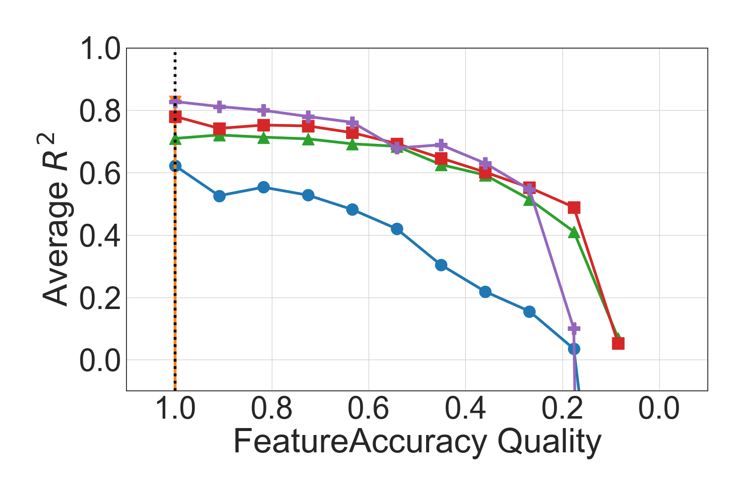
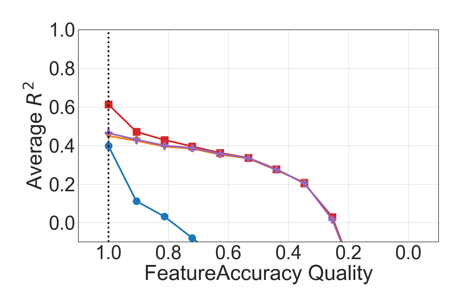
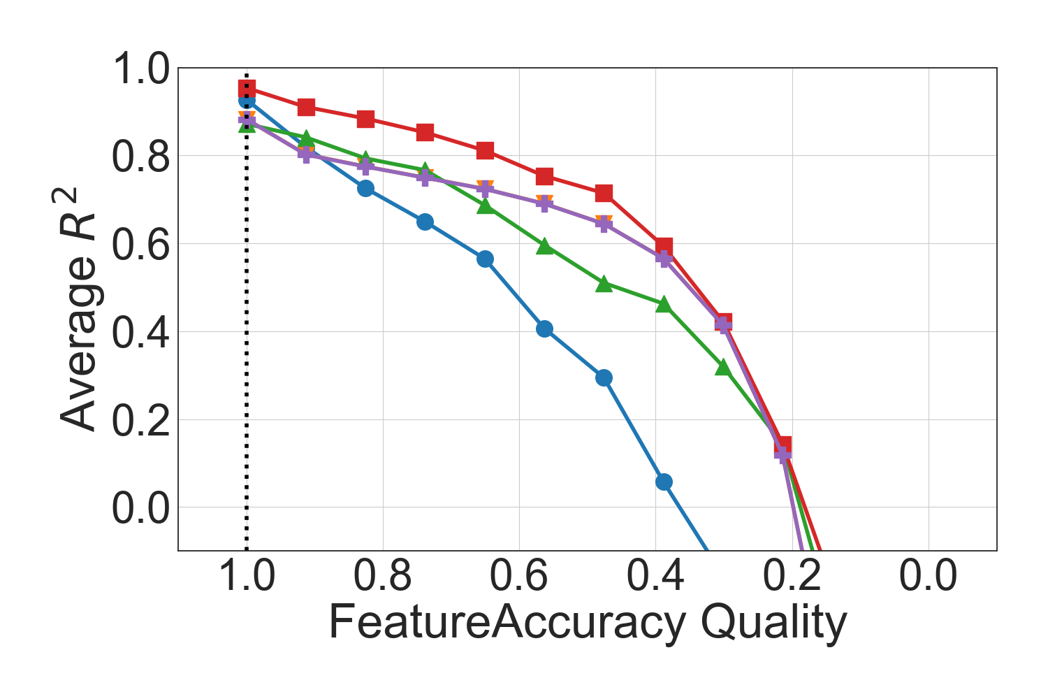
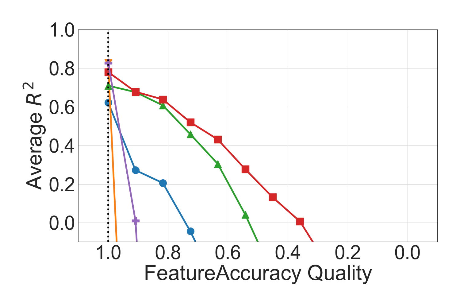
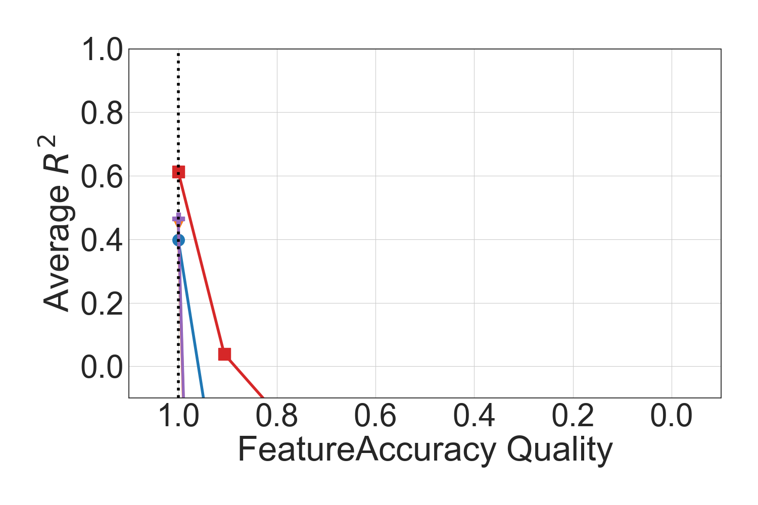
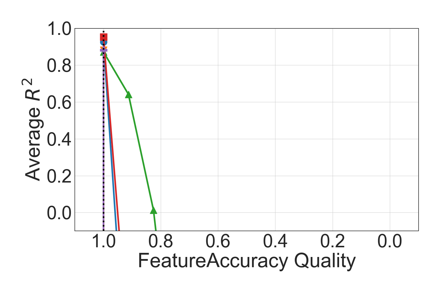
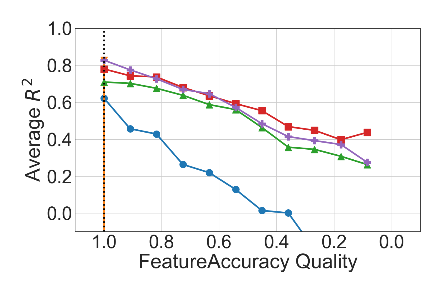
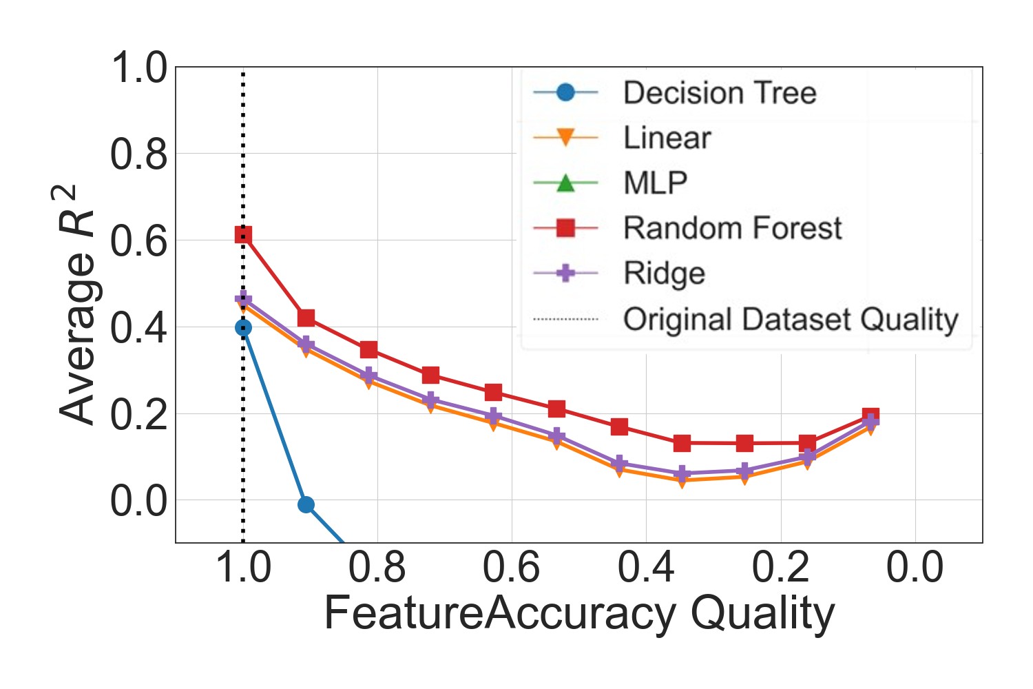
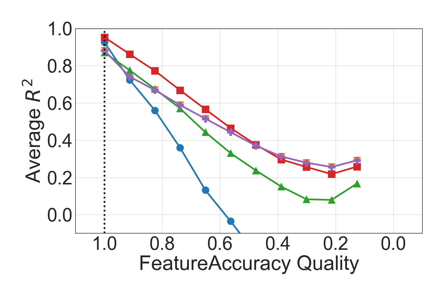
Decreasing feature accuracy causes a clear performance degradation of the regression algorithms in all scenarios, as shown in Figure 13. As for completeness, the degradation is the highest in Scenario 2 (Figure 13 in the second row) and having inaccuracy also in the training data, i.e., in Scenario 3, leads to a better performance (Figure 13 in the last row). RF and RR are the most robust algorithms in Scenarios 1 and 3 for all datasets. The performance of LR/RR sometimes decreases slower than that of RF. For RF, the robustness is a result of the ensemble. LR and RR benefit from the normal distribution of the noise. As the feature accuracy polluter adds normally distributed unbiased noise for numerical features, the underlying assumption still holds when applying pollution, leading to only a slow performance decrease in LR/RR. The sudden performance drop of LR on Houses in both scenarios, shown in Figure 12(a) and Figure 12(g), is due to the high number of features and low number of samples in this dataset, apparently leading to a high sensitivity regarding inaccuracy when computing a linear relation. The regularization of RR seems to solve the problem.
For Scenario 1, the performance decrease in RF and LR/RR is slower in higher quality ranges and faster in lower quality ranges as the differences between training and test set become too large. The behavior of the algorithms in Scenario 2 is similar but slower compared to the one showed in response to drop in completeness. In Scenario 3, those algorithms show more linearly decreasing performance, with a stagnation or even improvement in ranges of very low quality. Apparently, the inaccuracies in training and test set align when the pollution is high, leading to an increase after a performance minimum. The DT algorithm is more sensitive to feature accuracy drop than the other algorithms in Scenarios 1 and 3. We assume that this is due to DT being sensitive to changes in the data, without having the assumption of normally distributed noise like LR/RR. DT’s performance decreases especially fast on IMDB due to the high number of categorical features (8) compared to the numerical attributes (4). MLP is more robust than DT regarding feature accuracy, while the comparison to RF and LR/RR differs between scenarios and datasets. When comparing between datasets, it is noticeable that the effect of pollution is overall the strongest on Cars, which is the dataset with the smallest number of features, followed by IMDB.
Target Accuracy.
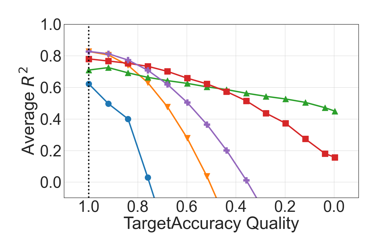
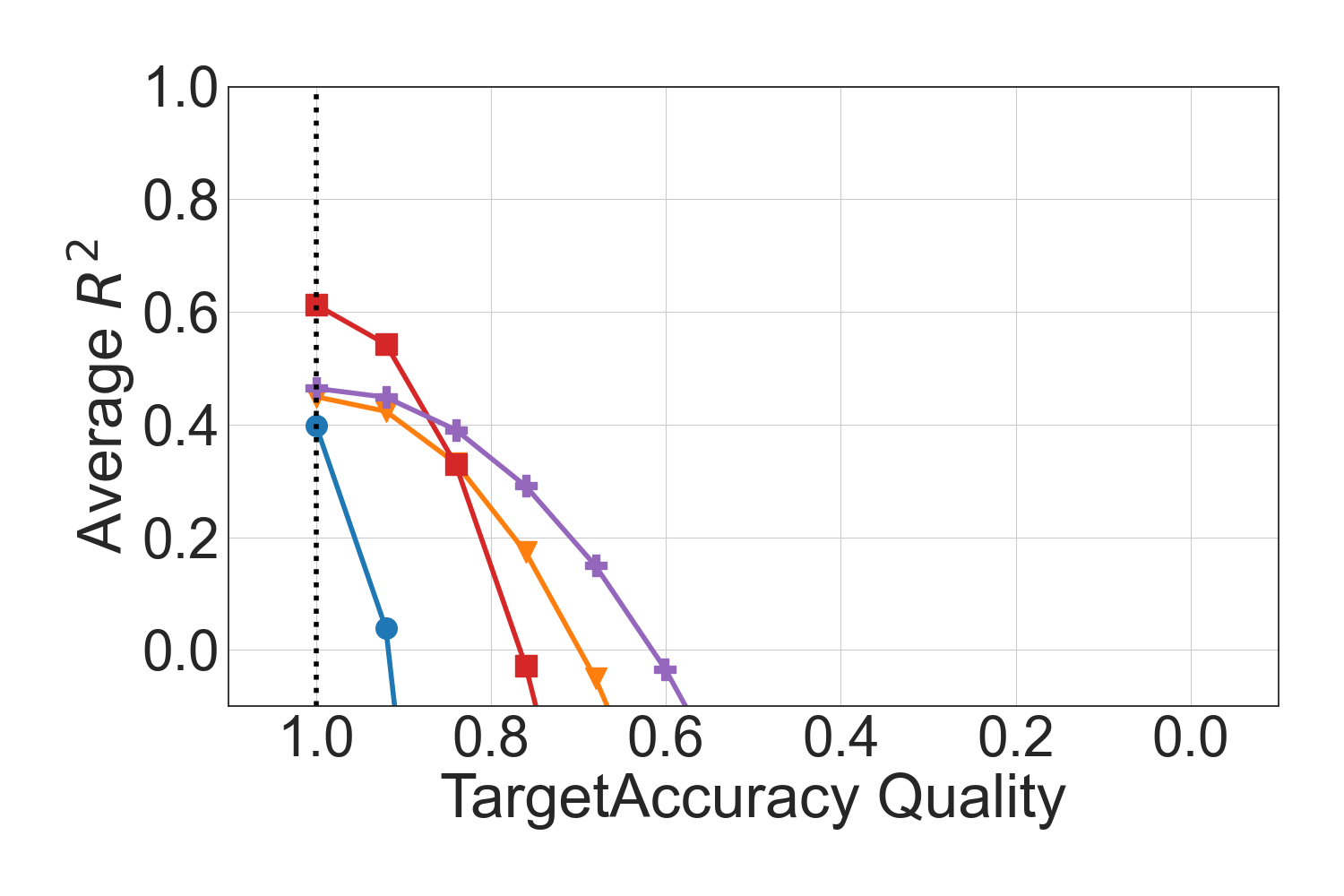
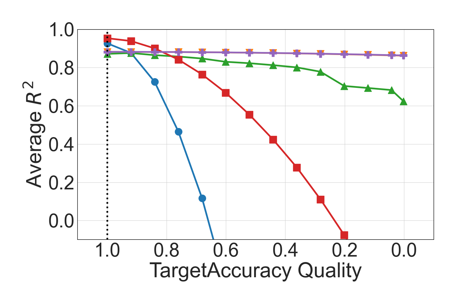
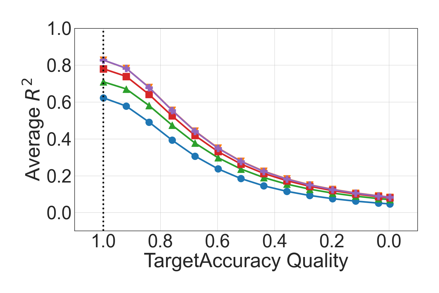
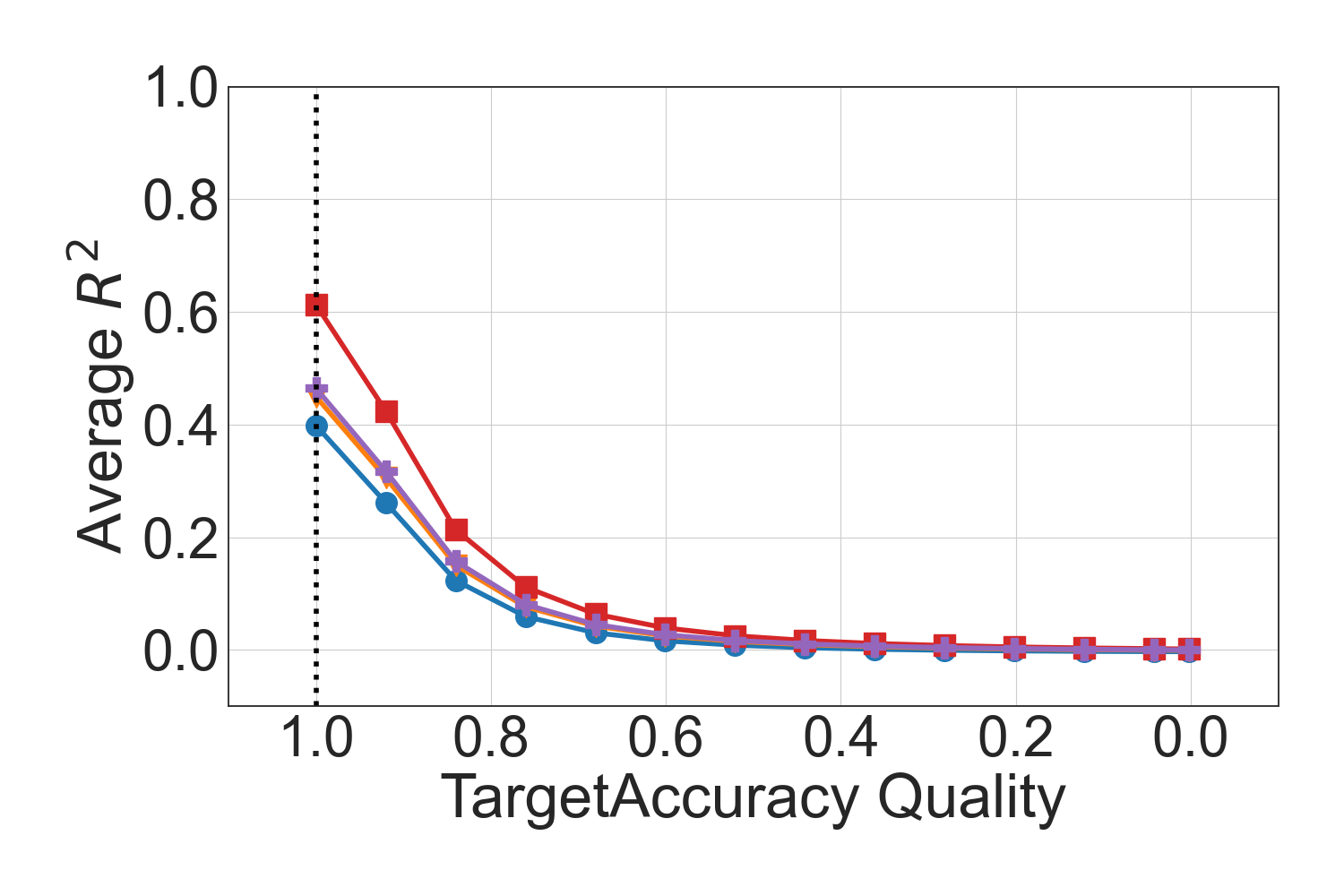
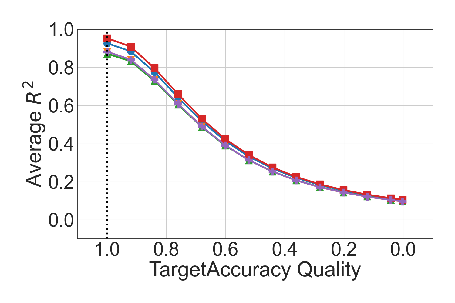
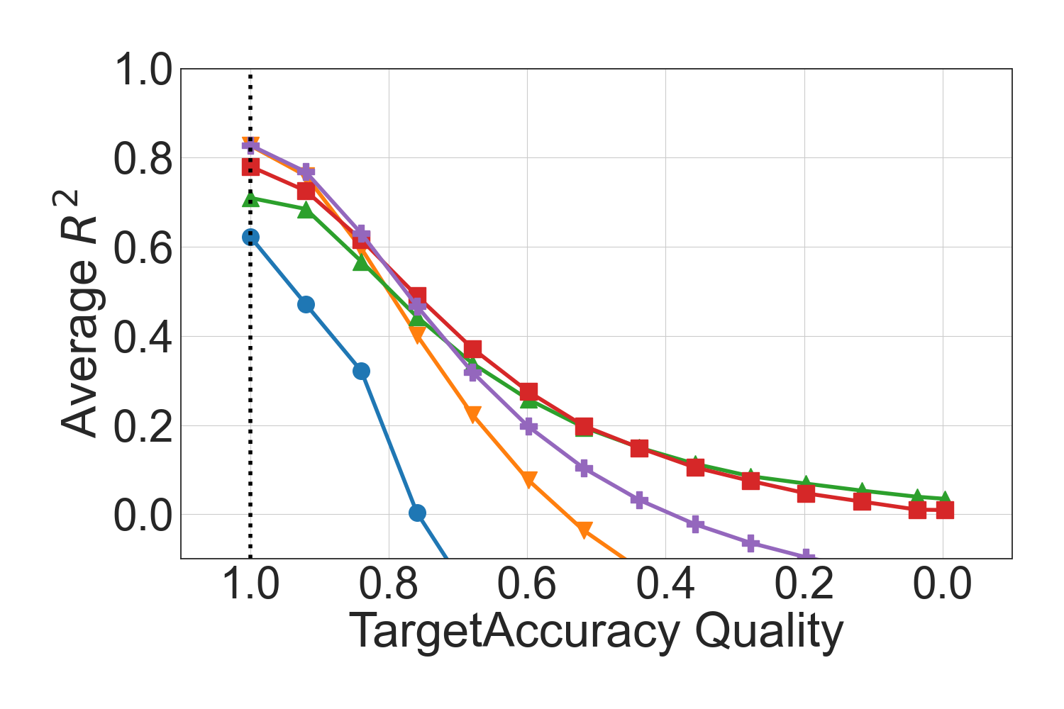
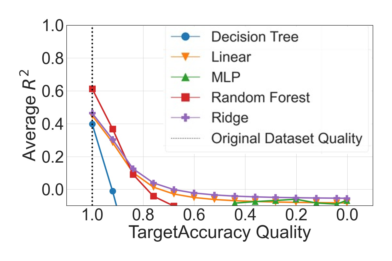
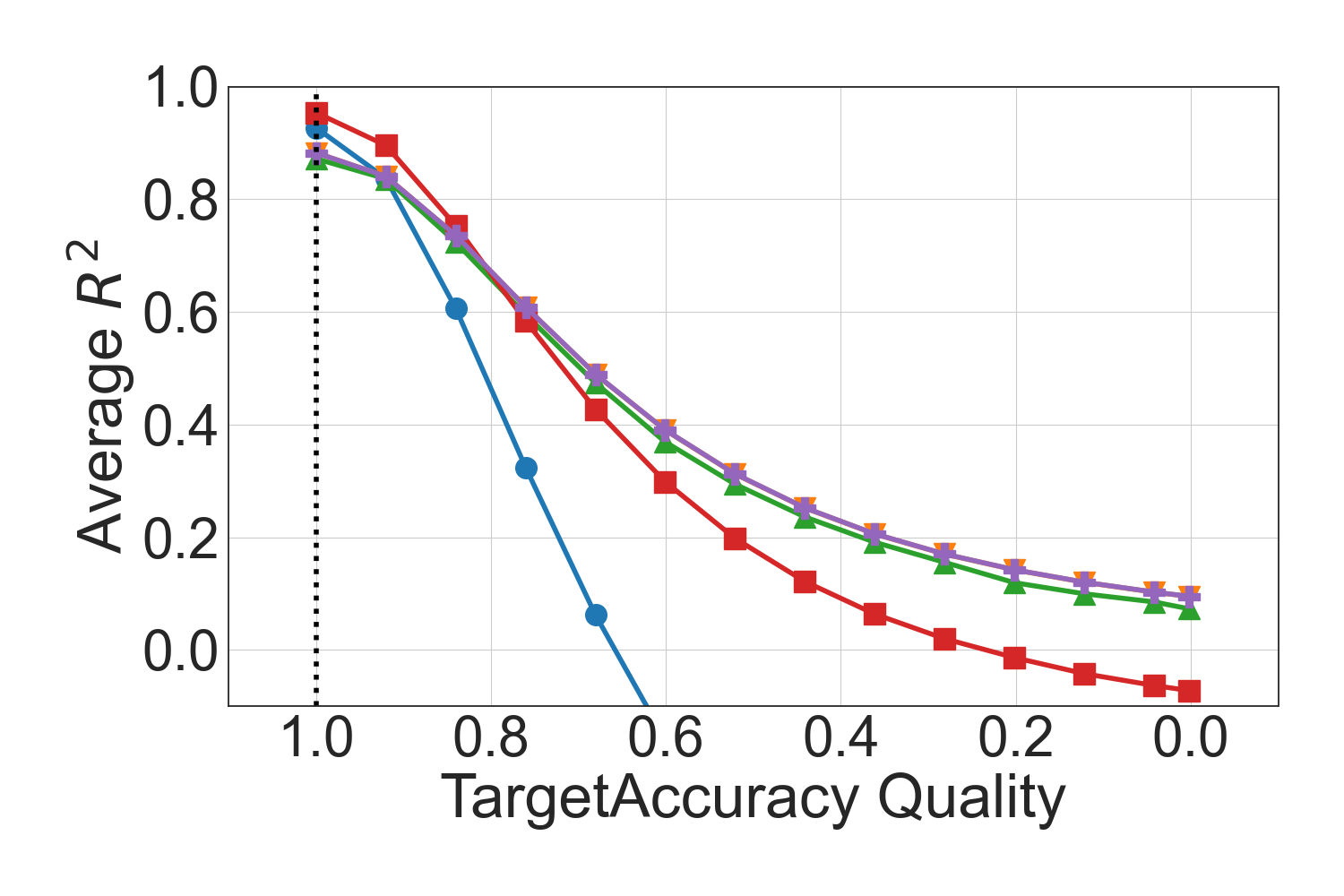
We observe a strong degradation in response to decreasing target accuracy for all datasets and in all scenarios, like for feature accuracy and completeness, but at a weaker level.
Scenario 1 (first row in Figure 14) shows the strongest degradation with different speeds for different datasets. For Cars (Figure 13(c)), having a low number of features and high number of records, we observe a heavy performance degradation for RF and DT, whereas the performance of LR/RR stays relatively constant as the noise is normally distributed. Thus, it does not influence the regression lines to such an extent that the performance decreases. In contrast, there is a degradation of LR and RR performance for Houses (Figure 13(a)) due to the large number of features with low sample size. In general, MLP is the most resilient model for low target accuracy. For IMDB (Figure 13(b)), it has a baseline performance below 0, and thus the effect of pollution is not considered here. For Houses and Cars, the MLP performs better than the other algorithms with increasing pollution. Comparing within the LR-based and the tree-based families: RR performs better than LR, and RF outperforms DT. Thus, the improved version of the algorithm performs better than the more simple version across all datasets. Contrasting Scenario 1 and Scenario 3 (lasr row in Figure 14), we see that the perceived performance, which is shown as Scenario 1, decreases faster than the actual performance, which is shown in Scenario 3, in higher quality ranges. In lower quality ranges, the perceived performance in Scenario 3 decreases slower or stagnates compared to Scenario 1. In Scenario 2, the performance declines gradually with the decrease in target accuracy, as the algorithms increasingly fail in predicting the emerging patterns caused by polluting only the test data. Comparing the pollution effect on the datasets, we see that the strongest degradation is present for IMDB. Cars and Houses dataset perform similar regarding this pollution method.
Uniqueness.
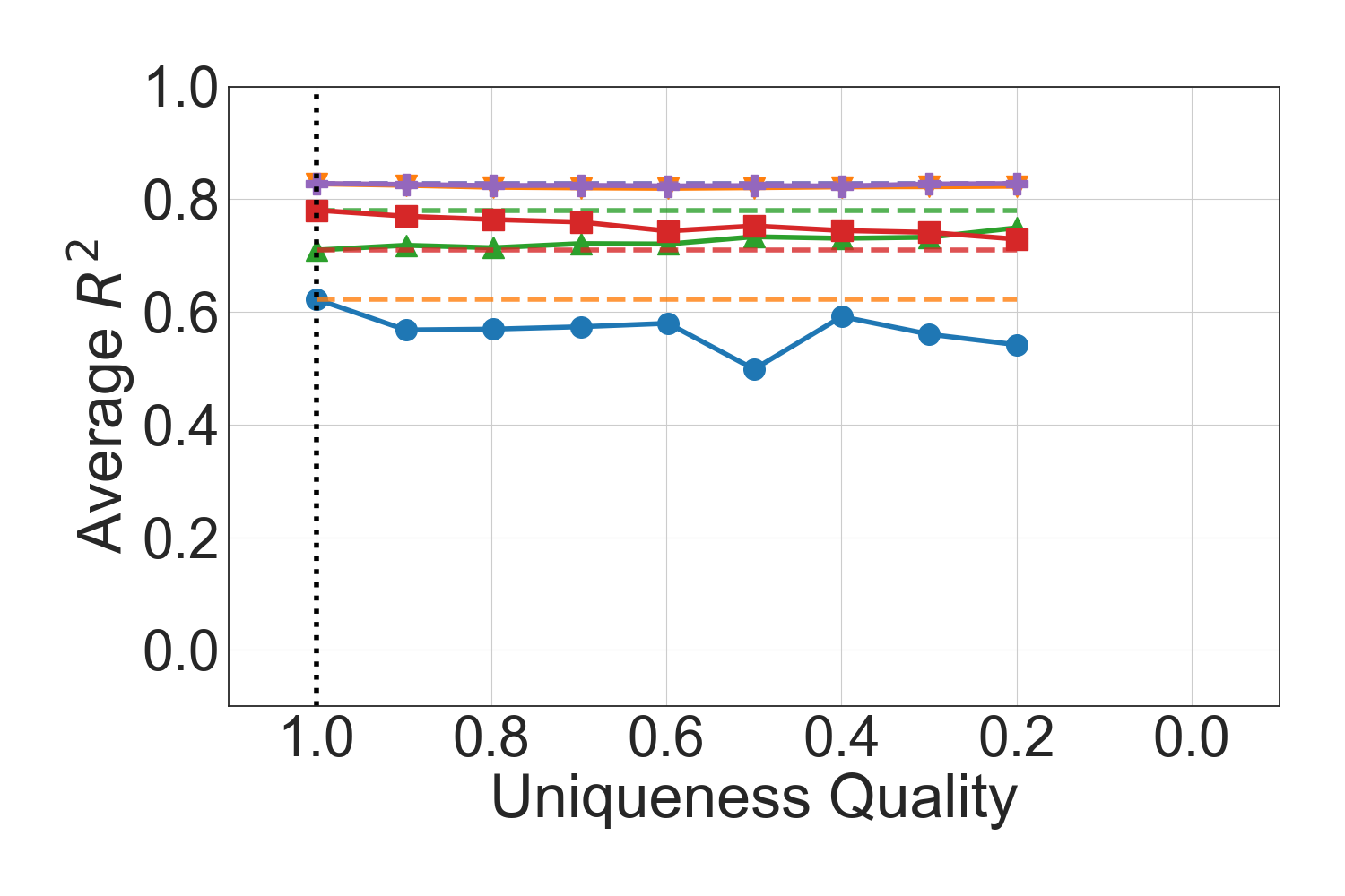
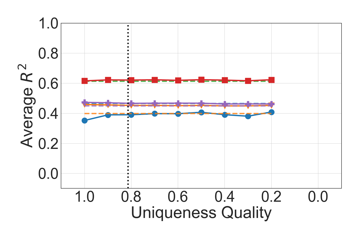
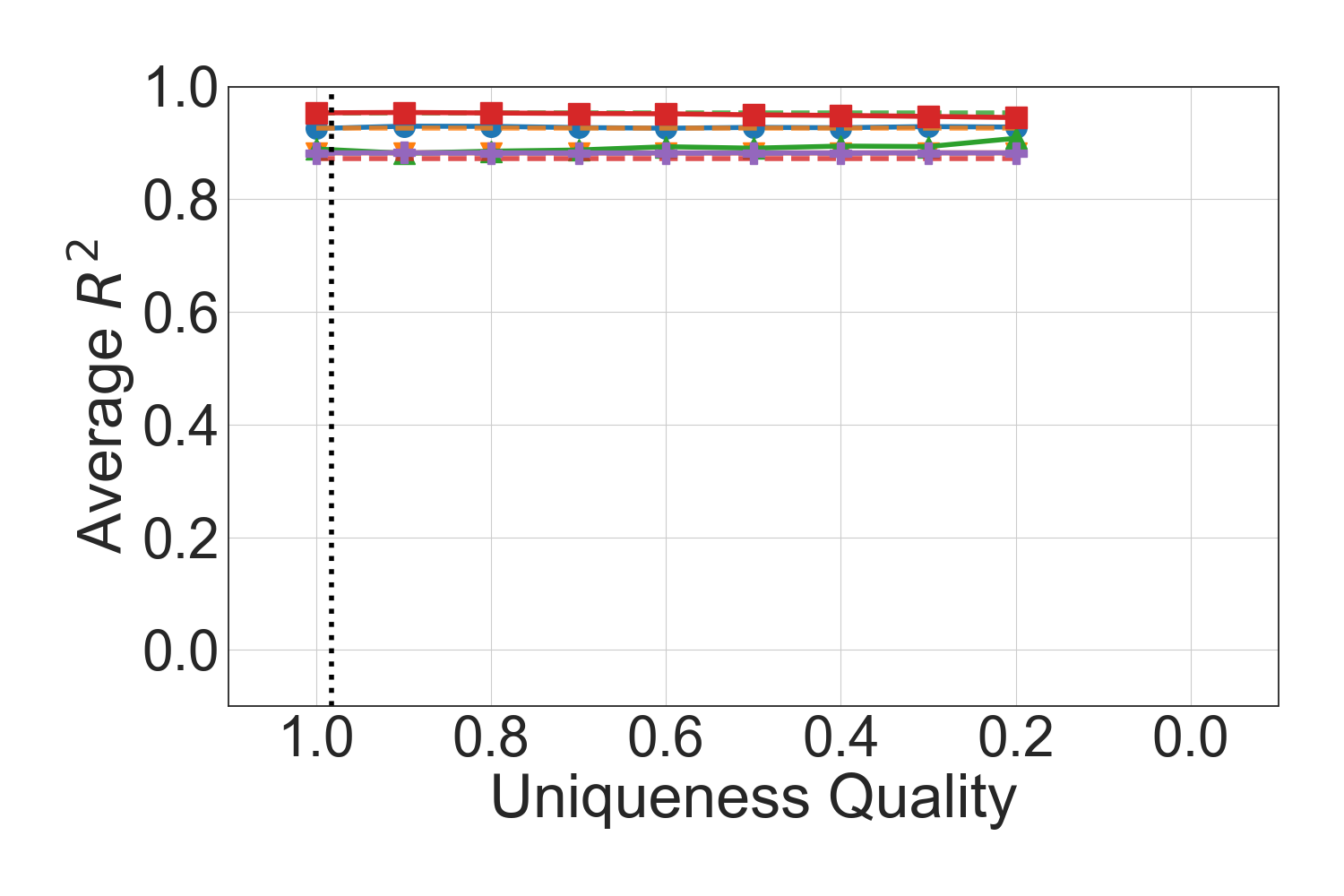
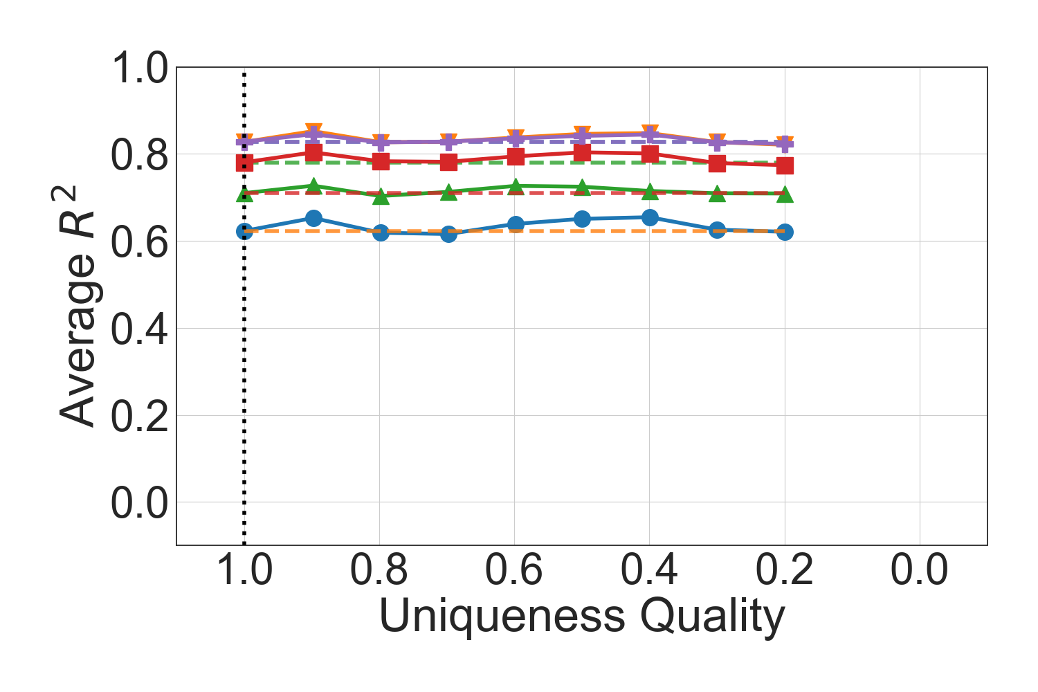
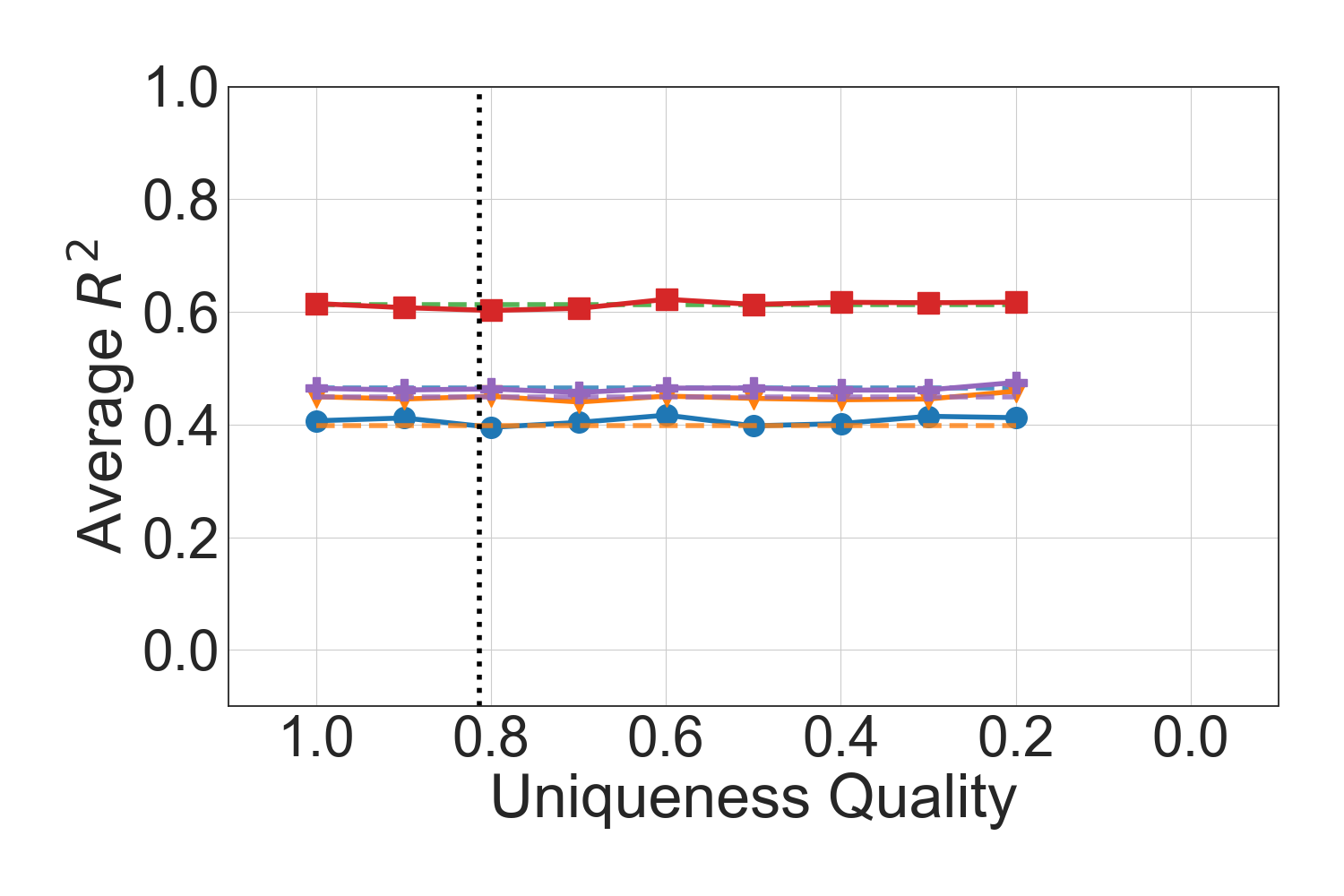
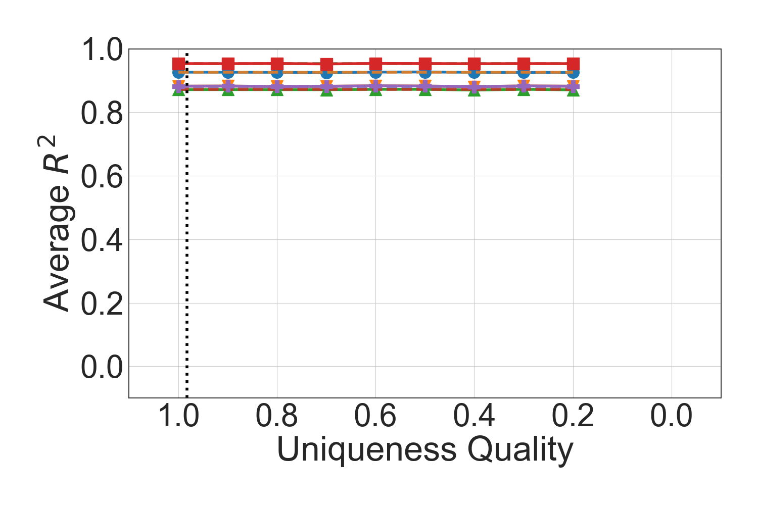
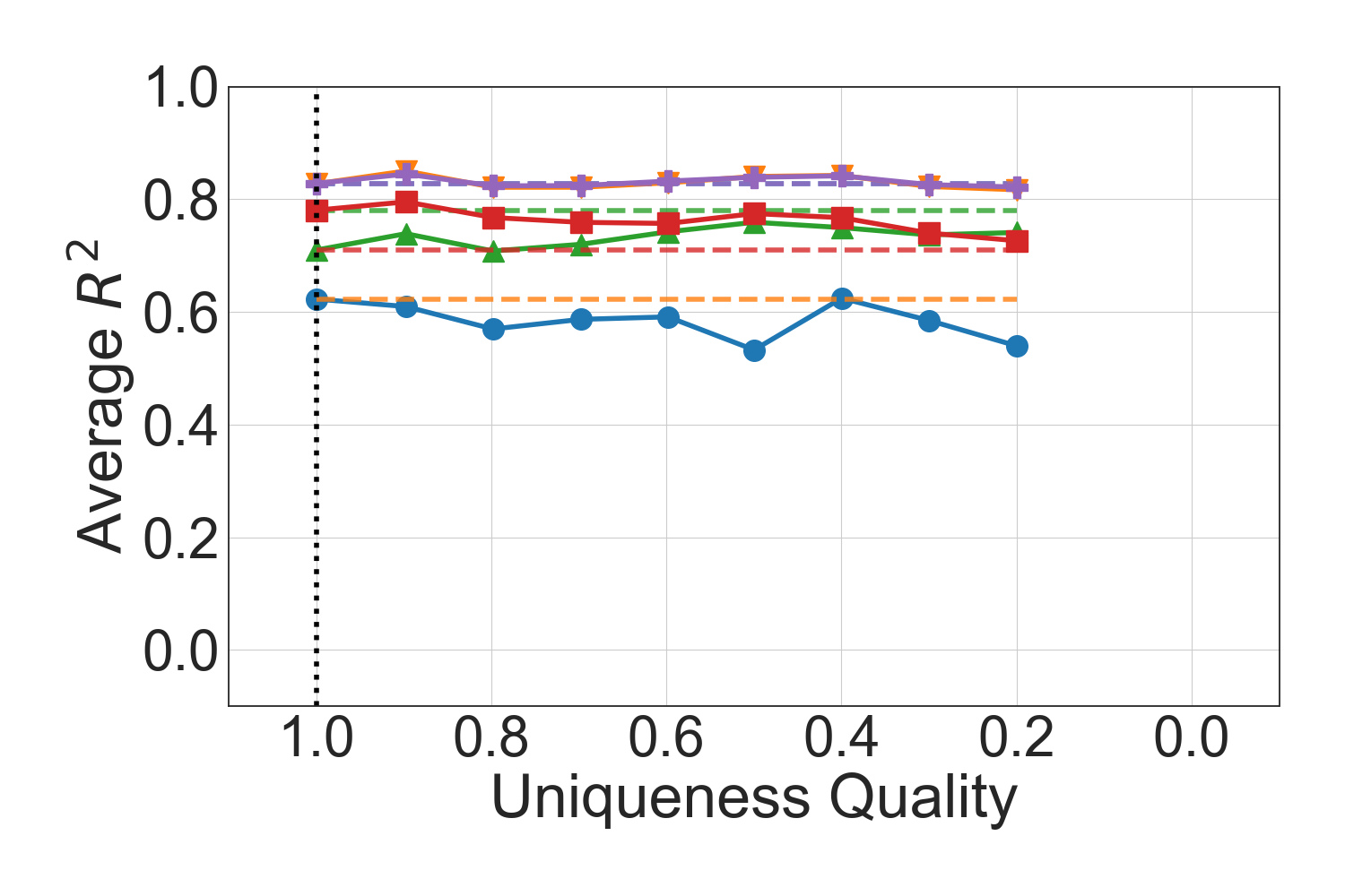
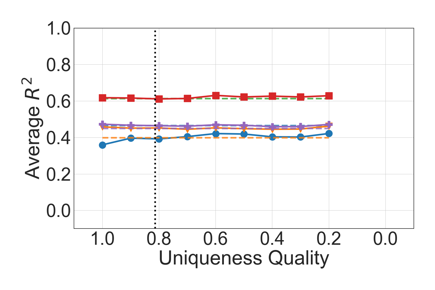
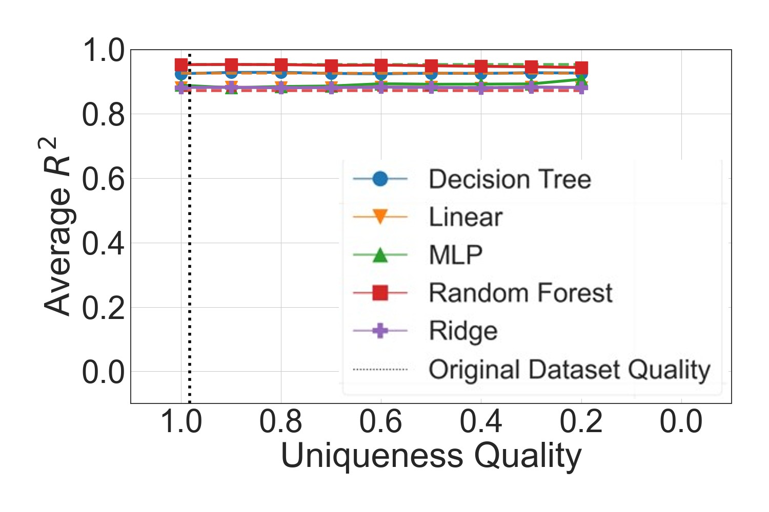
Decreasing uniqueness does not have a considerable effect on the performance of the algorithms, regardless of the scenario or dataset. On the datasets with many samples, we see no effect at all in Figure 15 where only one duplicate is added. Datasets with a small sample size, like Houses (Figures 14(a) and 14(g)), show a slight performance decrease with decreased uniqueness in Scenarios 1 and 3 due to an exaggerated influence of few samples on the training dataset, as they occur several times as a result of duplication. Comparing the uniqueness with duplicate count sampled by normal distribution (Figure 25 in the Appendix) and uniqueness with all samples having duplicate count of 1 (Figure 15), we do not see different behavior for Cars and IMDB. For Houses, inserting duplicates following a normal distribution causes a larger degradation of all algorithms’ performance, especially for Scenarios 2 and 3, as some samples appear regularly and thus have a relatively higher impact. As Cars and IMDB have fewer features and more samples compared to Houses, this explains the higher resilience of the algorithms.
Target Class Balance.
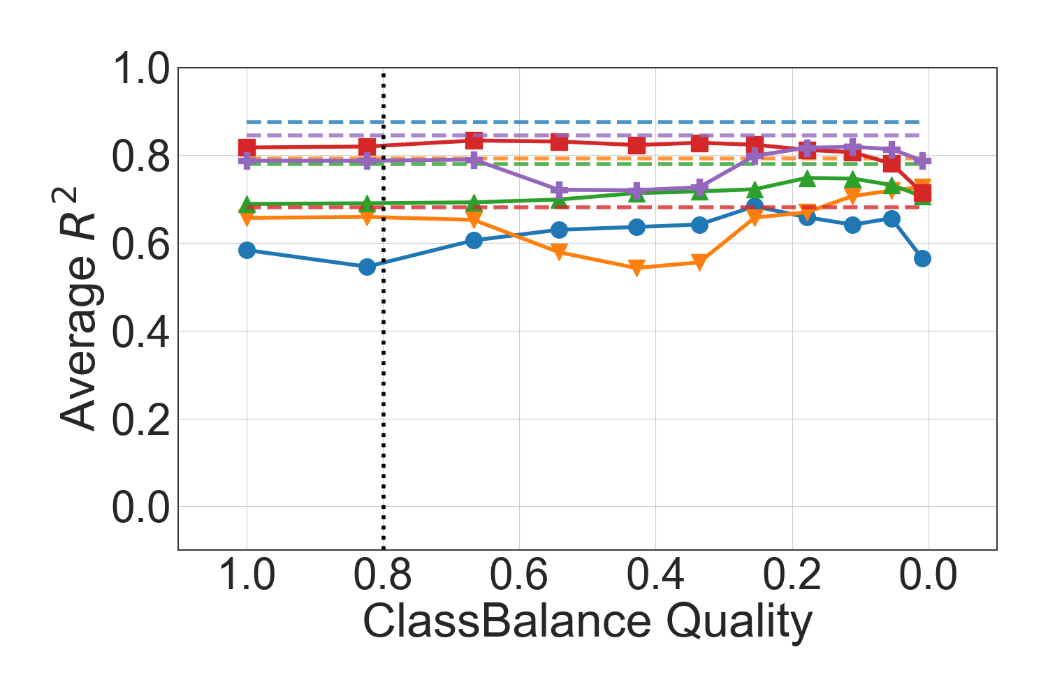
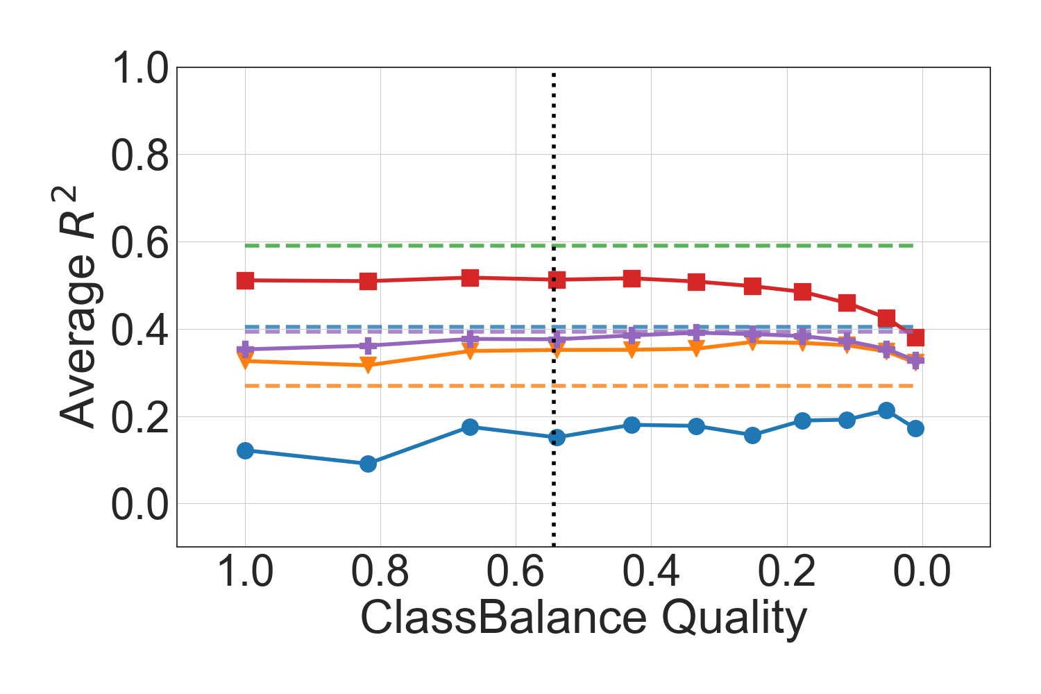
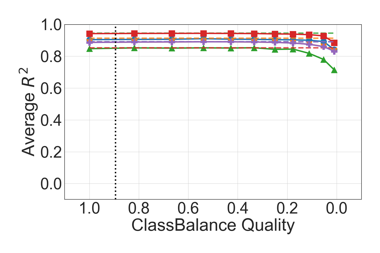
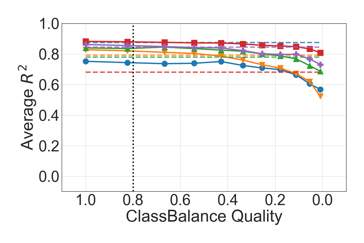
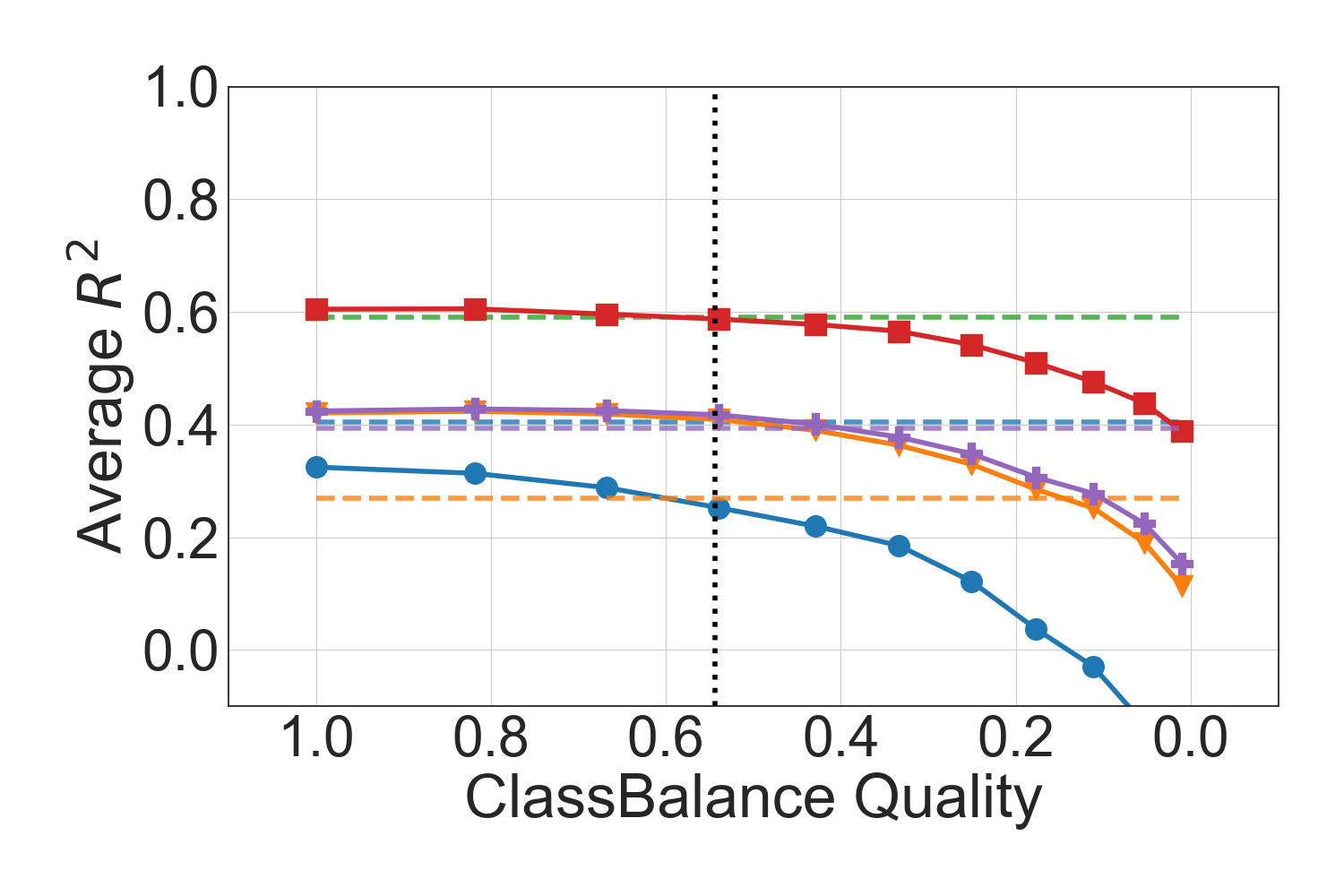
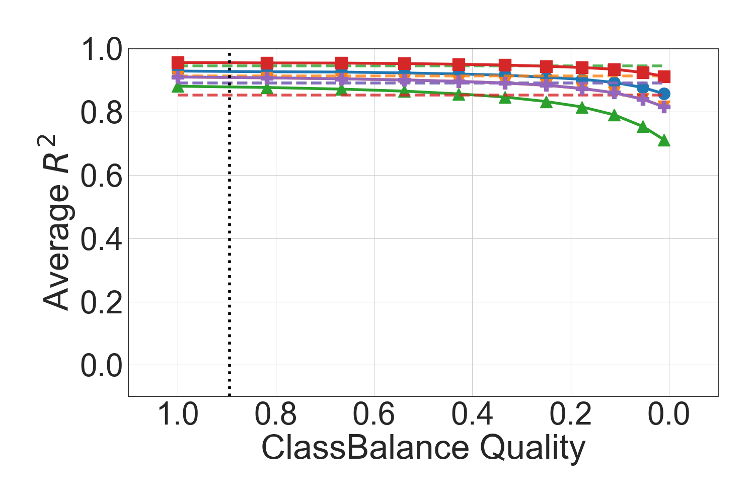
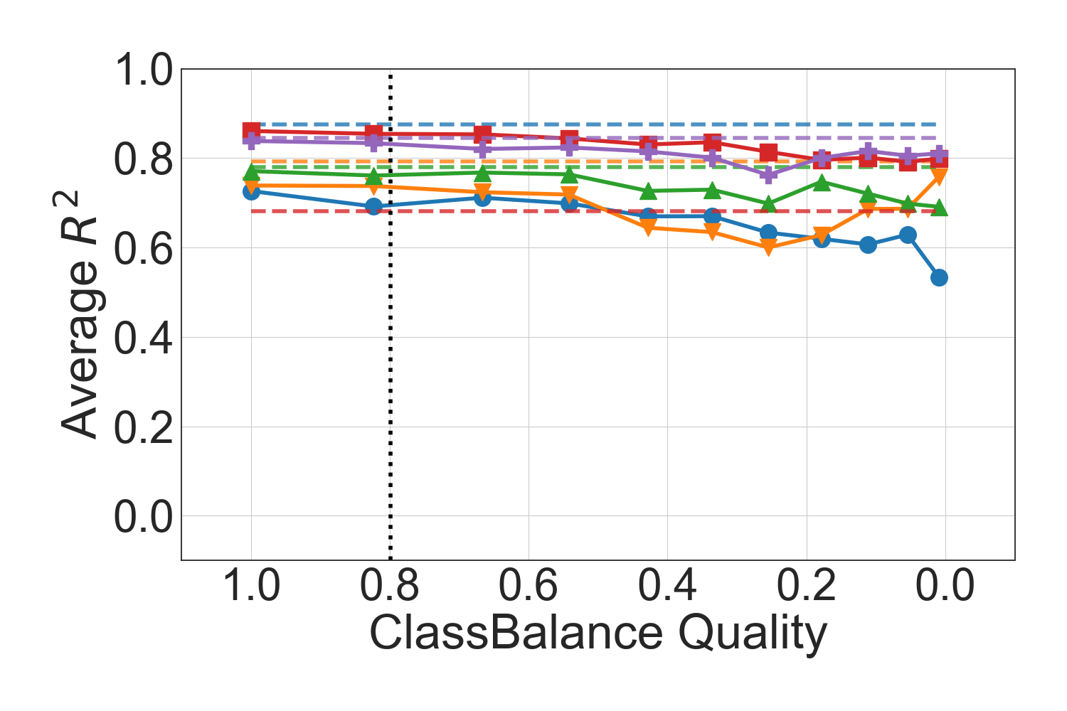
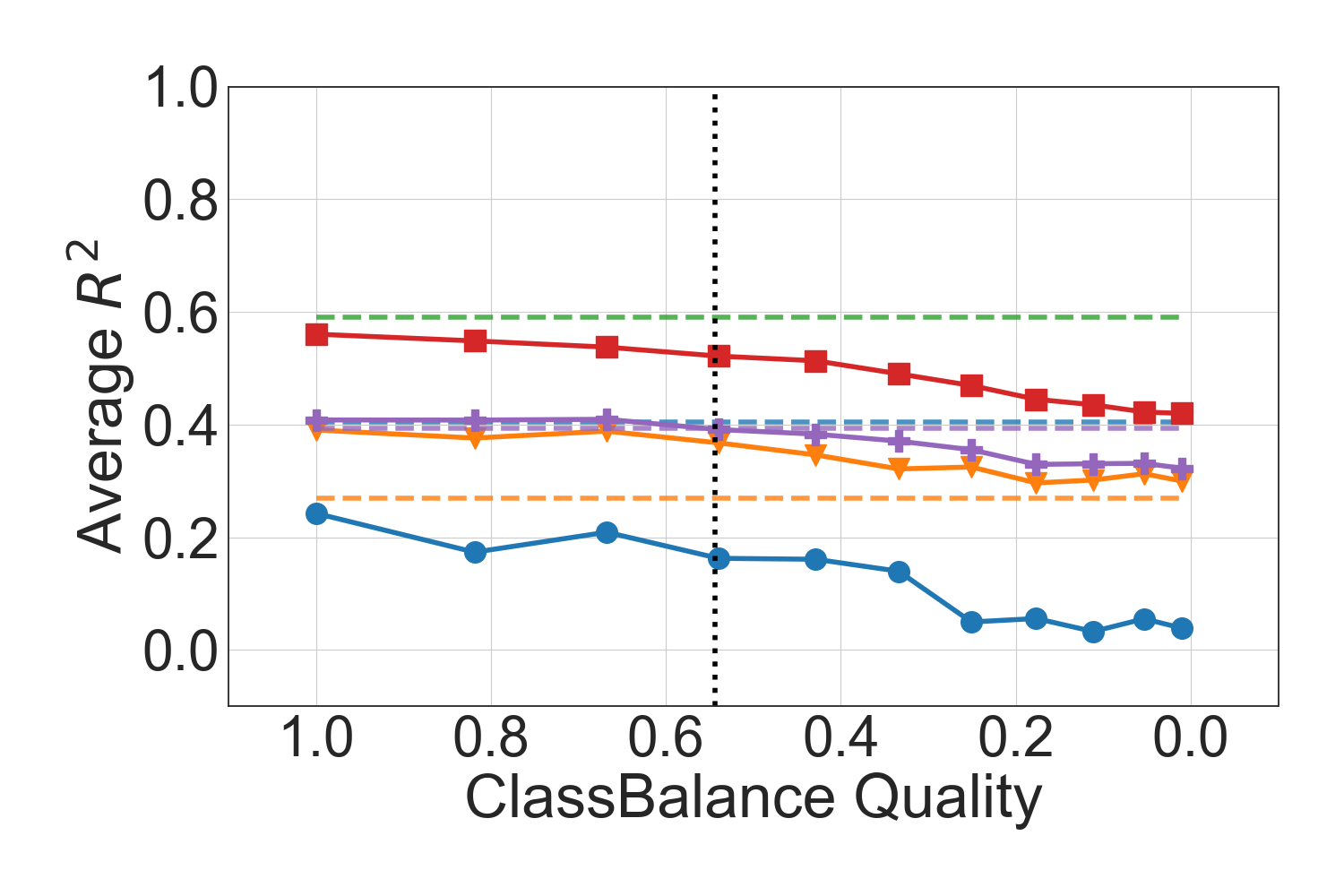
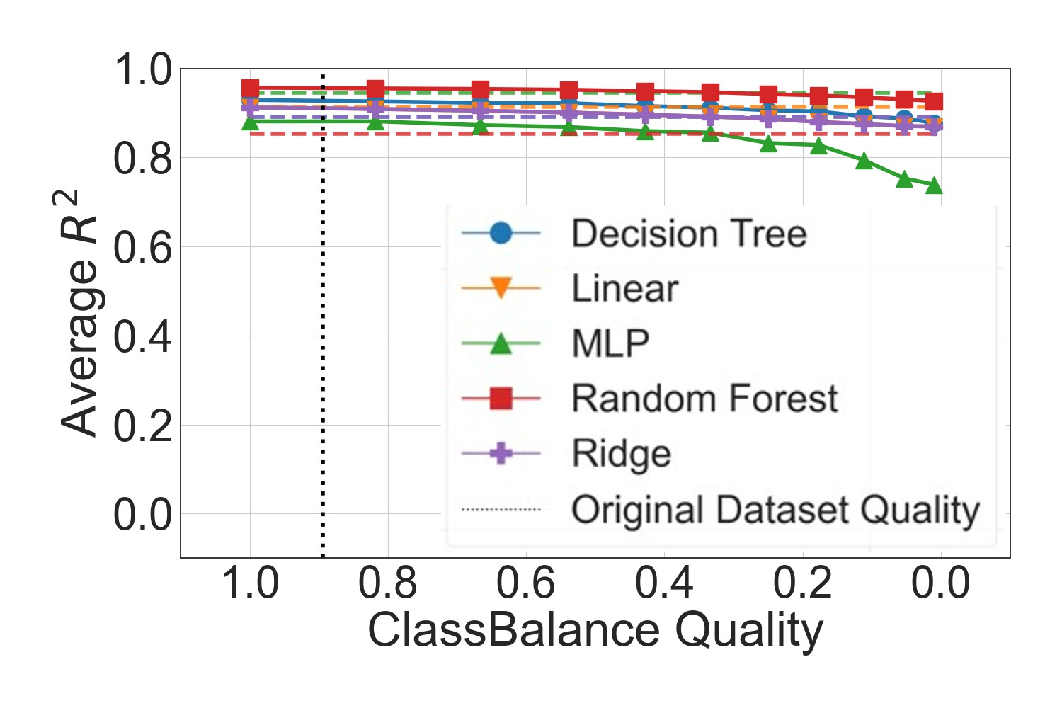
Similar to the uniqueness dimension, we observe a low effect of the target class imbalance increase in all scenarios on all datasets as shown in Figure 16. Two facts can justify this observation: First, regression datasets usually have a continuous target variable, i.e., a mostly normally distributed and therefore inherently unbalanced target variable. Second, we had to discretize the target feature and discard resulting classes with very few samples before applying pollution, as described in Section 5.2. Only with a high imbalance above 50%, we start to recognize a degraded performance of all algorithms. Even though there is no big influence of the pollution in general, we see similar behavior between algorithms. All five algorithms show the same relative degradation when decreasing the target class balance, and thus handle target accuracy similarly. Comparing the datasets, we see very similar responses to an increased pollution. The performance degradation on IMDB is faster than on other datasets, especially if the imbalance was introduced only to test data (Figure 15(e)). The effect on Houses is less than for IMDB. Target class balance has the lowest influence on Cars.
6.3 Clustering
Finally, we discuss here the effect of degrading the six data quality dimensions of three datasets, namely: Bank, Covertype and Letter on the performance of five clustering algorithms, namely: Gaussian Mixture clustering, k-Means/k-Prototypes, Agglomerative clustering, OPTICS and Autoencoder. All plots shown are scaled to share the same y-axis. This comes at the downside of Bank plots having a lower readability, as the algorithms’ performance is significantly worse on this dataset than on the others. For versions of Bank plots where the y-axis was scaled more towards the needs of this particular dataset, please refer to Figure 27 in the Appendix. Here, we start by some general notes and observations which are beneficial for the discussion in the rest of this section. Bank is not originally designed for the clustering task, very low in dimensionality and contains a high amount of duplicated data points. Upon further research, we found that some combinations of the two categorical features dominate the data, with the combination of job = blue-collar and marital = married being found in about of samples and the combinations’ technician, married and admin., married together making up another approximately of the samples. Therefore, we know that large parts of the data are not distinguishable by anything but the age feature. We question this feature’s impact, as it is likely dominated due to the One-Hot Encoding adding more dimensions to the data. As this encodes the categorical values in the data into one dimension per value, it distinguishes the impact of each individual dimension, which disproportionately affects the age feature which is not encoded in this way. Therefore, we are aware that the clustering quality on Bank is expected to be low. We argue that this is not an issue in most cases, as we can still derive some relative changes in clustering quality and argue about the impact of any given quality dimension regarding this dataset. However, we also believe that the findings on Bank are to be taken with a grain of salt and more weight should be put into findings on Covertype and Letter. We observed that the Gaussian Mixture algorithm assumes data that follows a single distribution, i.e., the random peaks and drops in its performance are caused by its sensitivity to the distribution of samples. This is particularly noticeable in those cases where large changes to either the data itself or the chosen samples are made by a pollution method. Bank is drawn from a mixture of Gaussian distributions. Thus, the algorithm behaves better on Covertype and the best on Letter.
Consistent Representation.
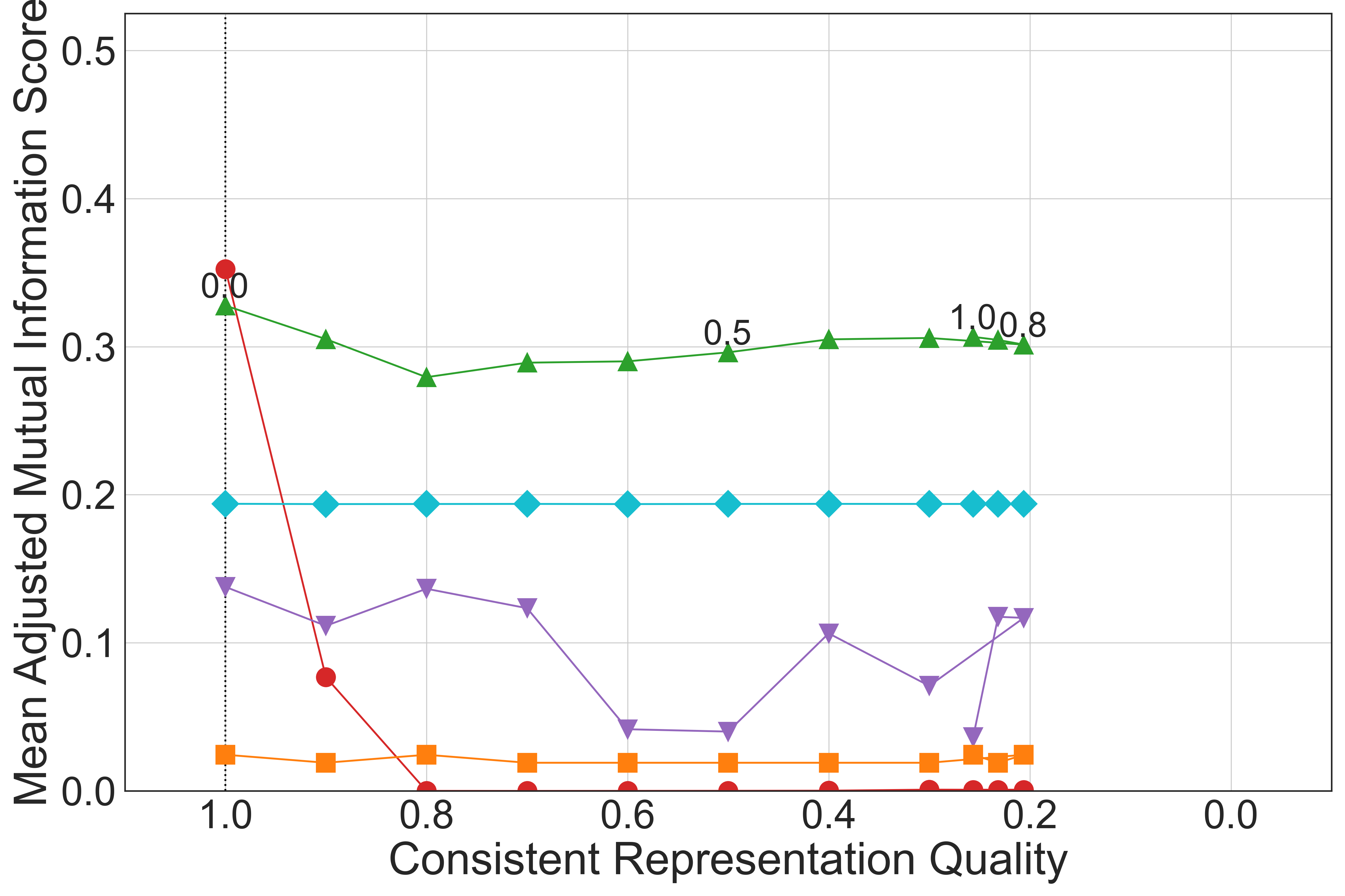
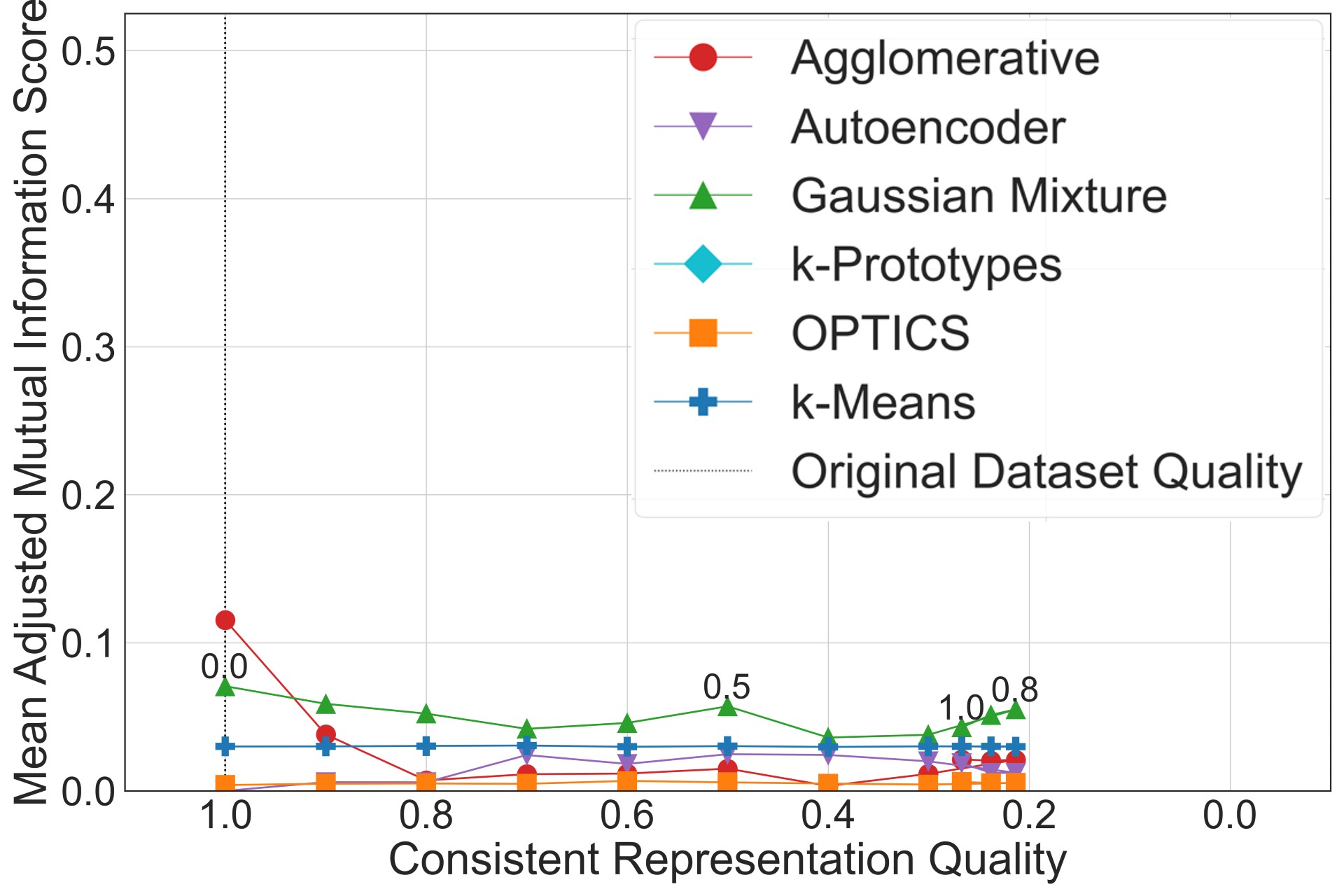
As previously mentioned in Section 5.4, Letter is the only dataset that the consistent representation polluter cannot be applied to, as it does not contain categorical features. This is why we only show two plots in Figure 17 (Figure 26(b) for focused version of Bank). For the interpretation of these two plots, it must be noted (as mentioned at the beginning of Section 6) that the percentage of polluted samples is indicated by extra numbers on the plot line of the Gaussian Mixture clustering. Each of the plot lines can make a kind of “backward step”, since they are oriented towards this percentage. We also only consider those consistent representation pollution results that generated four additional representations per categorical value, not those adding only one new representation per value. Figures 16(b) and 16(a) indicate that the performance of the k-Means / k-Prototypes and OPTICS algorithms is not affected by the degrading consistency of Covertype as well as Bank. In contrast, the Agglomerative algorithm is strongly impaired even with only a small pollution degree. This susceptibility arises because the algorithm uses a Boolean distance matrix to represent differences between values for categorical features rather than a distance matrix with actual distances like for numerical features. This make it easy to disturb the bottom-up combination process by altering the representation of the values. I.e., with a quality measure of , the Agglomerative clustering algorithm encounters enough distant samples which are far enough removed from the original samples of their clusters, that they form their subtrees which may not be merged into the main cluster trees during the bottom-up combination process before we cut off the tree structure at our desired number of output clusters. Additionally, this can also cause clusters which were initially separated to now be merged before these outlier subtrees are merged, therefore also degrading the quality of clusters which used to be correctly identified.
For the Autoencoder approach, we suspect that its observed random behavior is due to the randomness of the neural network training and its dependence on the sampled data for each of the five runs, which is amplified in datasets with many features like Covertype. The Gaussian Mixture algorithm’s performance slightly decreases on average with decreasing dataset quality. This general reduction is in a similar range for both Bank and Covertype, with a performance difference of about 0.02 between the unpolluted (baseline) and fully polluted variants of the datasets. We attribute the unexpected results (initial decrease, then increase in AMI) to the observation made at the beginning of this section.
Completeness.
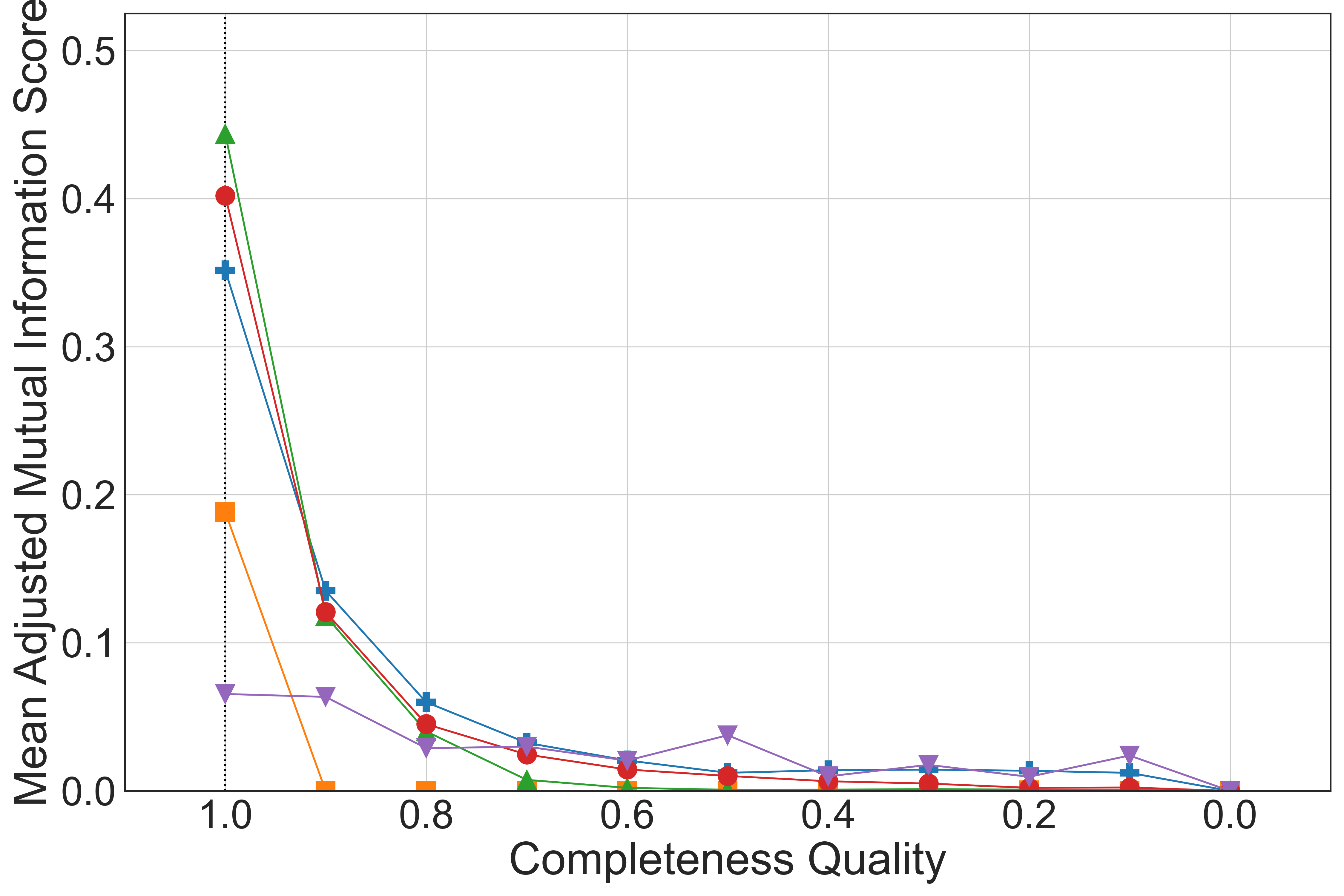
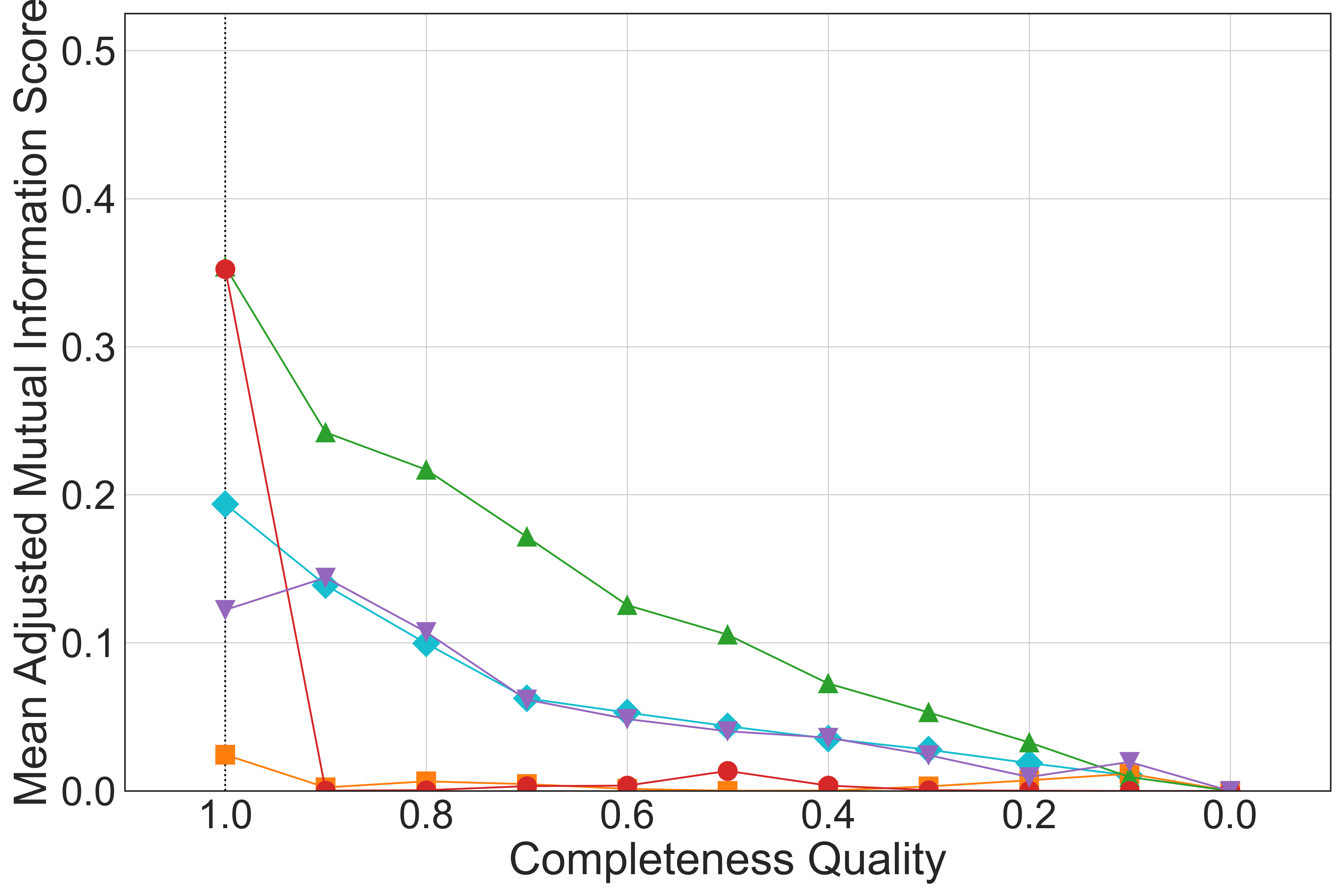
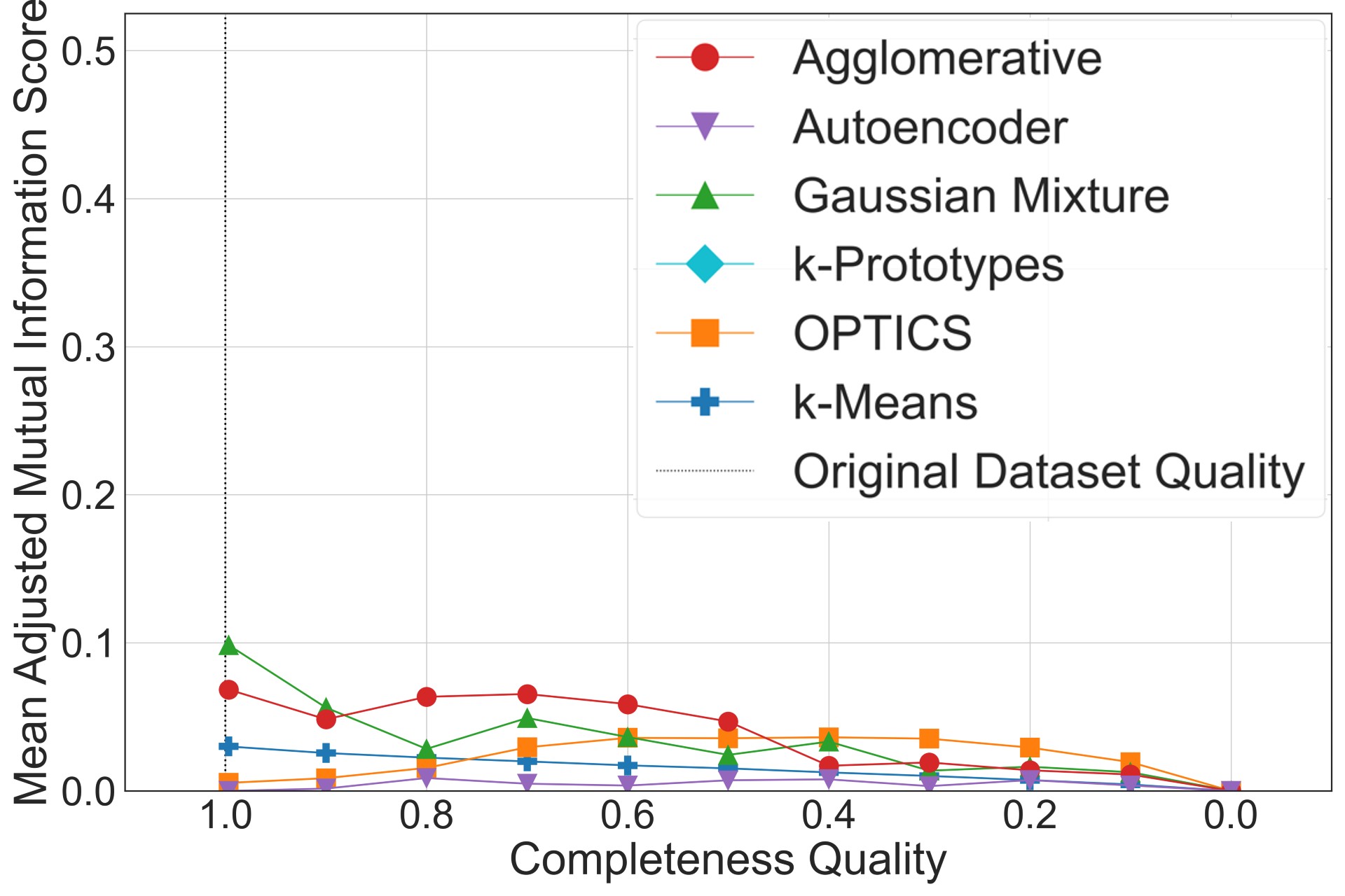
For all datasets, we notice in Figure 18 a decline in average AMI for all algorithms as the completeness decreases. While the different datasets show differing behavior, this general trend stays true among all of them. In Figure 17(a), depicting the results on Letter, we can see that this decline is rapid and approaching zero in a negative exponential fashion. Nevertheless, the Autoencoder seems more robust against the insertion of default values. The OPTICS algorithm is most affected by a degradation of the dataset completeness, only identifying one cluster at a completeness quality of already (Figure 25(a) in Appendix). We believe this to be due to the shifting of data points from their original clusters to outlier clusters, where data points group due to their equality in the inserted default values. This both decreases the density of existing clusters and creates a new, potentially high-density cluster, which may skew the OPTICS algorithm’s perception of the expected density of clusters in the dataset. Yet, for Covertype (Figure 17(b)), the Gaussian Mixture, Autoencoder and k-Prototypes algorithms performance degrades almost linearly and in a slightly slower fashion compared to other datasets. This is because of the high number of categorical features that are more resilient against the insertion of default values. This hypothesis is strengthened by our findings on the low dimensional Bank (Figure 17(c)), which also contains categorical features and is more resilient against clustering performance degradation than Letter for the completeness quality dimension. For the OPTICS algorithm we observe an almost identical behavior to Letter, however, it does recover some performance on low-quality datasets. This does line up with the peak of clusters identified by the algorithm (Figure25(b) in Appendix), leading us to believe that this small increase in clustering quality is simply a coincidence with the algorithm having identified smaller clusters that, by chance, match up with parts of the original clusters in the data. As shown in Figure 17(b), the Agglomerative algorithm drops almost to zero at a completeness of . We attribute this behavior to the default values added to represent missing values in the dataset. The added placeholders are not values found in Covertype for either the numerical or categorical features, as there are no defaults for empty or unknown given in the original data. This can create small clusters of outliers far away from the rest of the data points. This effect is exacerbated by the one-hot encoding, where new dimensions are created for the placeholders introduced into the data, aligning all datasets with inserted defaults along these dimensions. The outliers may be so far away from the original data points, that the Agglomerative clustering method does not merge them into an existing cluster with original data points in it before it is forced to return the clusters found. This has two effects. First, there are now clusters of outliers that likely do not share any resemblance to the original clusters in the algorithm’s output. Secondly, clusters previously correctly identified in the original data are now merged as the number of clusters returned is fixed and are therefore no longer correct. For Bank, we can observe the overall decline in performance for all but the Autoencoder and OPTICS clustering approaches (Figure 17(c) or Figure 26(a) in Appendix), generally matching our expectations derived from the previous two datasets. The OPTICS and Autoencoder algorithms’ clustering performance generally matches the shape of the curve produced by the average number of clusters identified by the approaches (Figure 25(b) in Appendix). The behavior of the Gaussian Mixtures as well as Agglomerative algorithms is justified by the issues with Bank in general and the Gaussian Mixtures algorithm’s particular restrictions regarding the data distribution mentioned at the beginning of Section 6.3.
Feature Accuracy.
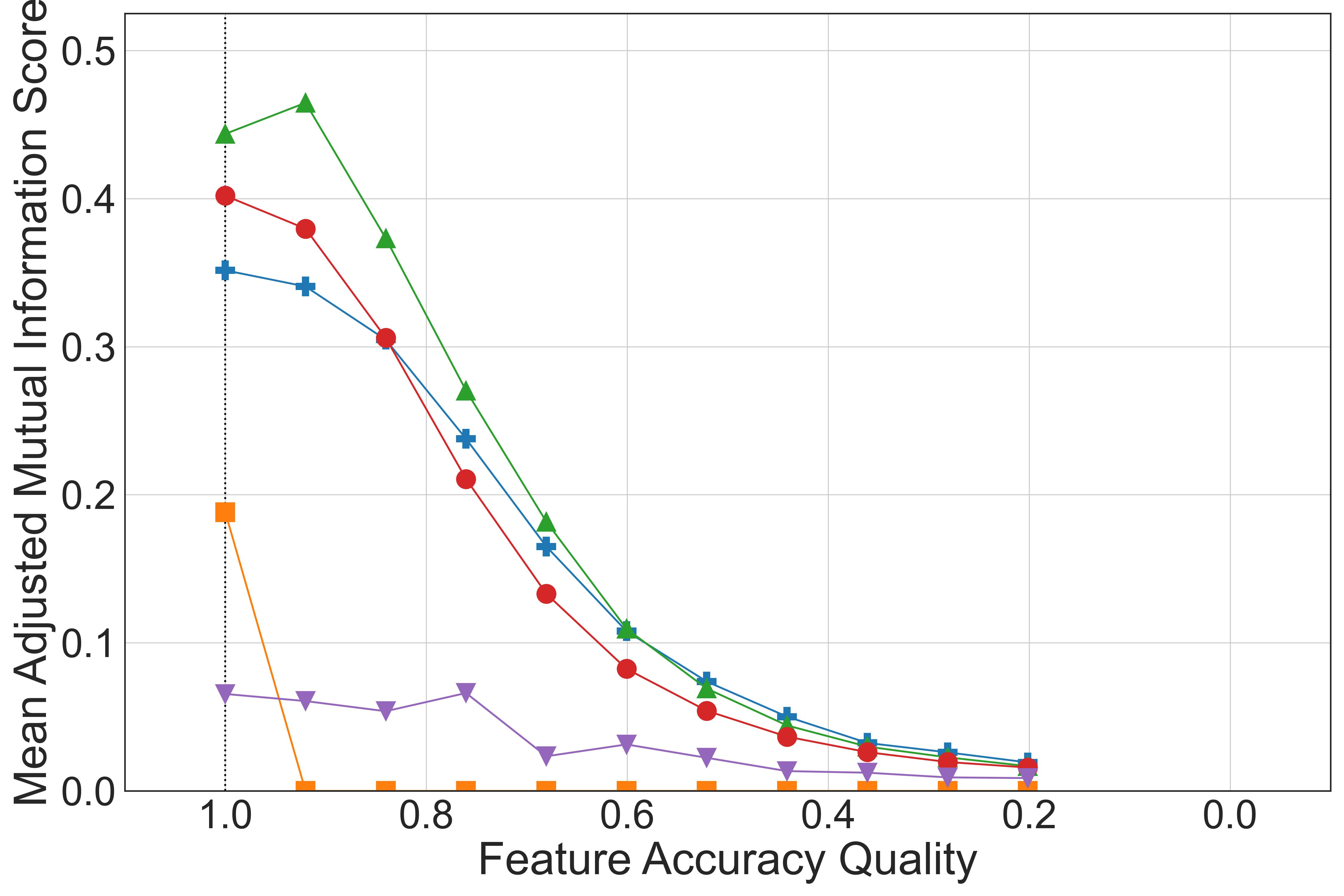
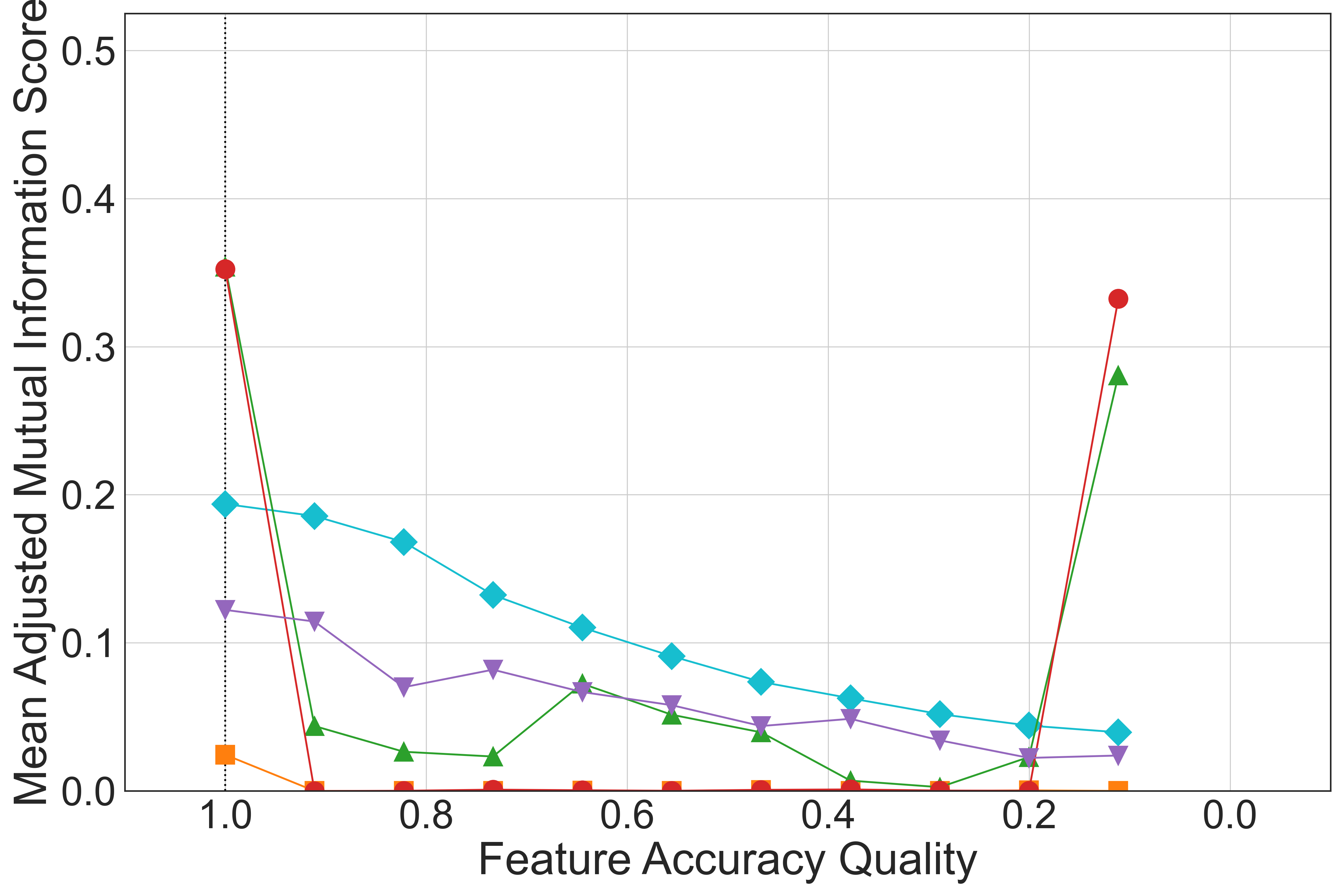
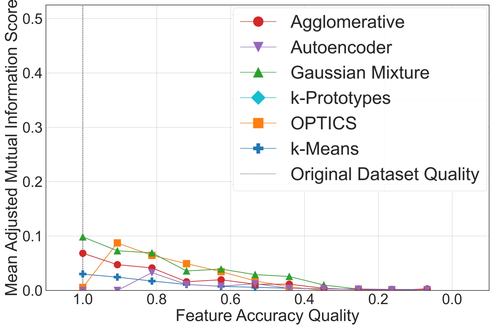
For Letter, consisting of only numerical features, we observe a very uniform decrease in the AMI score when decreasing the dataset feature accuracy for almost all algorithms (Figure 18(a)). This is due to the normally distributed noise we apply to numerical features degrading their accuracy in a gradually increasing fashion, continuously decreasing the distinguishability of individual clusters by spreading out their points more and more. In addition, we can observe a slight improvement in performance for the Gaussian Mixture algorithm in the first step of the pollution (i.e., for an aggregated feature accuracy quality of ). We suspect this to be caused by the addition of noise, bringing the data closer to the assumed underlying mixture of Gaussian distributions. Moreover, we assume that the performance of OPTICS decreases at the first step of the pollution as the noise causes the density to approach a uniform level rapidly, reducing the cluster distinguishability and unifying them to a single cluster when viewed from only a density perspective (Figure 25(g) in Appendix).
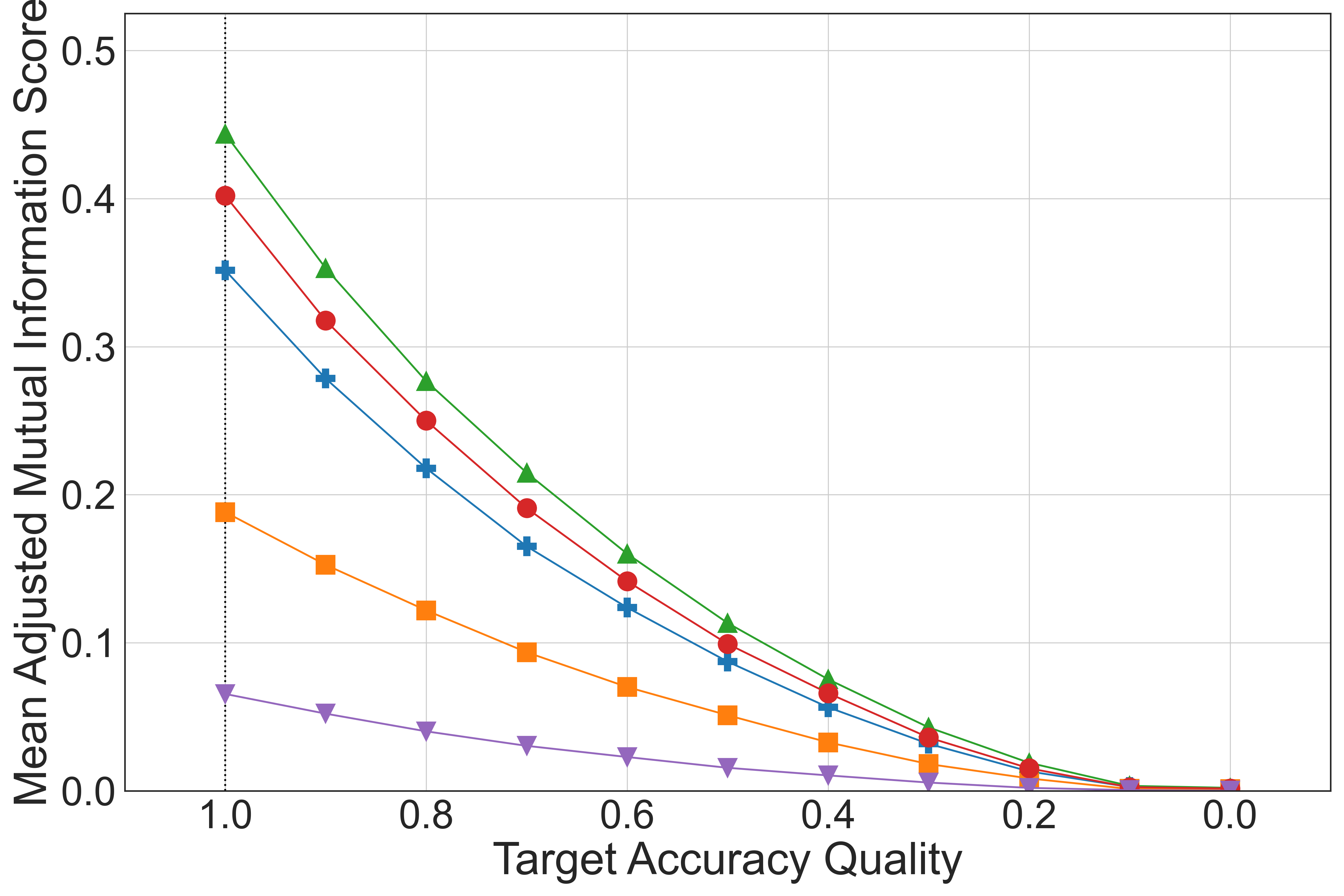
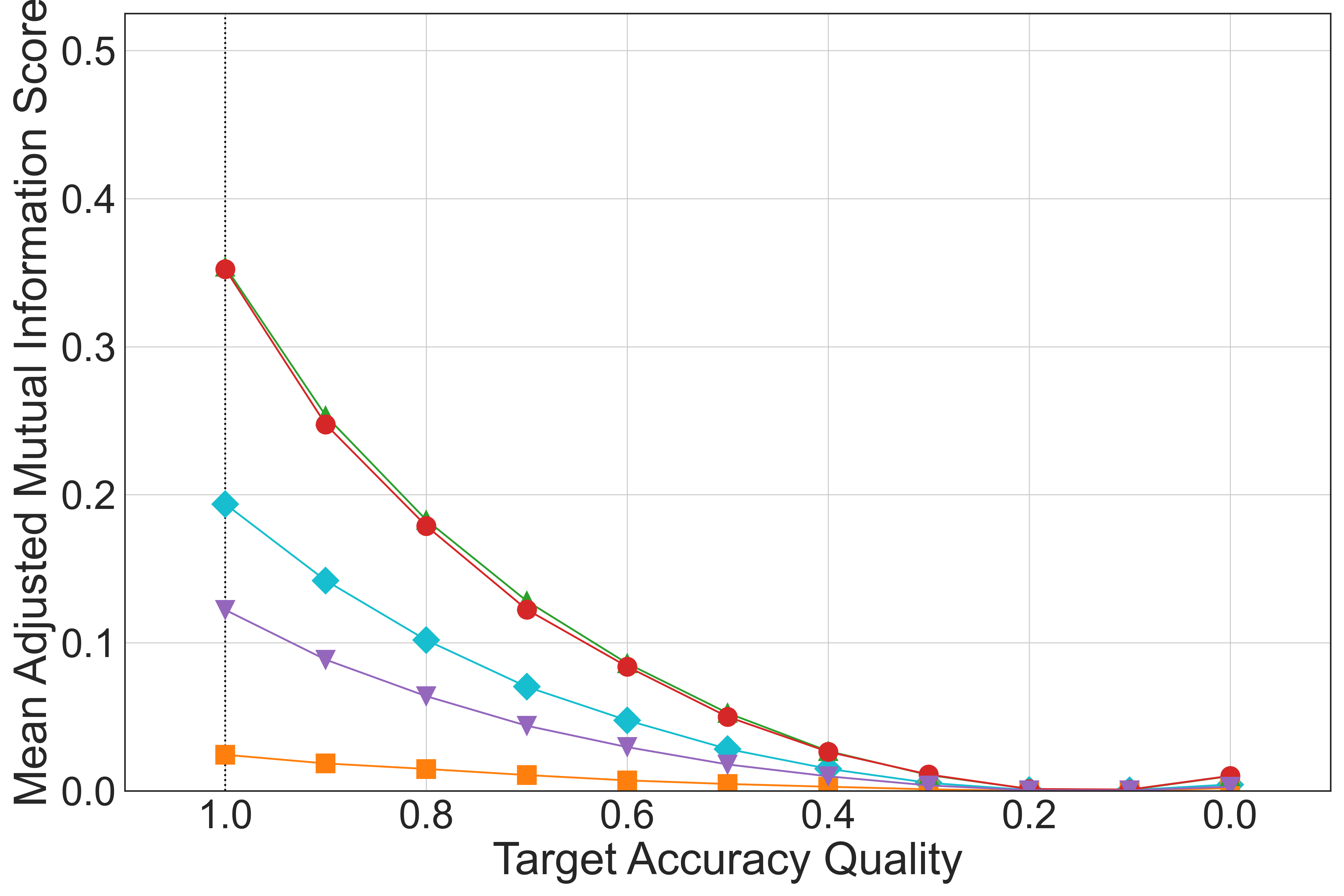
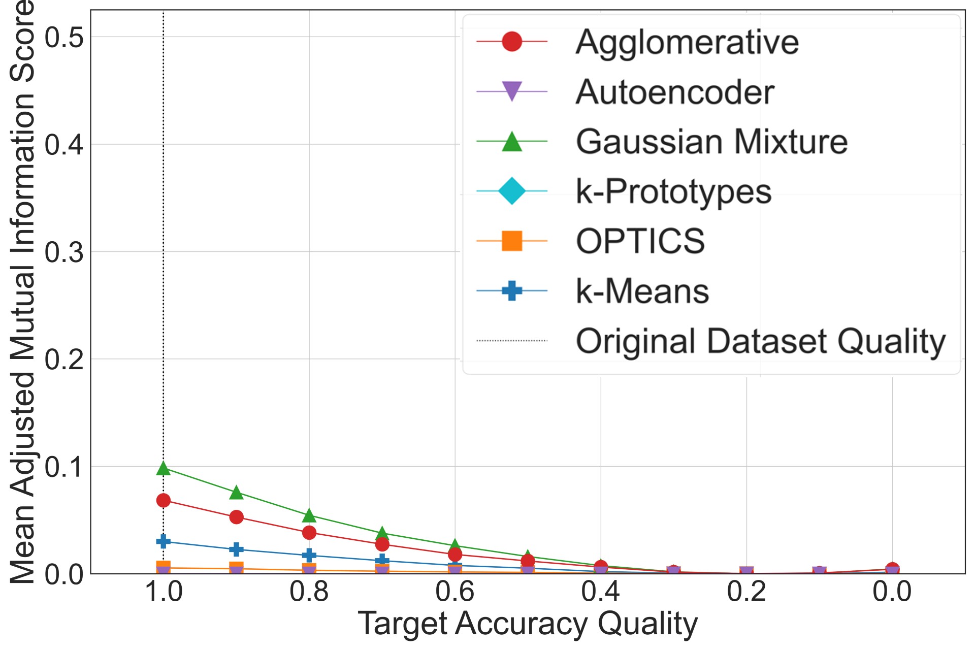
In Figure 18(b), the Gaussian Mixture algorithm exhibits a special behavior at the maximum pollution : it almost reaches the AMI score achieved on the clean dataset: Covertype consists mainly of binary features that have been completely inverted in its fully polluted version. Therefore, the dataset contains mainly the same information as before the pollution. The slight difference in performance comes from the ten remaining numerical features, which do not share the same information at any two points of the pollution. To investigate why the performance of Gaussian Mixture clustering on Covertype improves slightly around a feature accuracy quality of about requires further research. Here, we expected a behavior more similar to that of the Agglomerative clustering approach. The Agglomerative algorithm behaves similarly, dropping heavily in performance as the pollution starts and spiking again at full pollution, but here the drop is again justified by the approach’s sensibility to outliers created in the high-dimensional space. However, unlike Gaussian Mixture, it shows a near-constant performance while it does not produce usable results on the polluted datasets, which is in line with our expectations. Consequently, both the Gaussian Mixture and the Agglomerative algorithms cannot meaningfully interpret datasets that have mainly binary features and has low feature accuracy. OPTICS behaves similarly on Covertype and Letter. In contrast to the explanation of OPTICS’ behaviour with Letter, here we assume that OPTICS forms small clusters of very high density in a few dimensions, causing the majority of samples to become outliers (Figure 25(h) in Appendix). The Autoencoder and k-Prototypes show an almost linear decrease in AMI score, which is not as rapid as the quality degradation for Letter when its feature accuracy is attenuated. In Figure 18(c) (or focused Figure 26(c) in Appendix), we can see the effect of the feature accuracy polluter on Bank. The performance increases for the OPTICS and the Autoencoder approaches in the first and second step of the pollution are striking. Looking more closely at the number of clusters OPTICS finds at a quality of (Figure 25(i) in Appendix), we see that OPTICS found two clusters in the original dataset and 24 clusters now. Therefore, we assume that OPTICS profits from very dense clusters, created by the high number of duplicates in this dataset, being broken up in this first step of the pollution. This is due to the added noise and the higher variance of the data introduced by removing duplicates through pollution of some of their values. With the Autoencoder, on the other hand, you can see that it achieves an increasing AMI score as long as not all the searched six clusters have been found. From the point where the Autoencoder has identified the desired six clusters, its performance decreases similarly to that of the k-Means algorithm. This descent is probably due to producing false clusters or more outliers. Like the k-Means algorithm just mentioned, the Agglomerative clustering and Gaussian Mixture algorithms also experience a consistent degradation of their results when the feature accuracy is increasingly lowered. This decrease is less rapid for Bank than for Letter.
Target Accuracy.
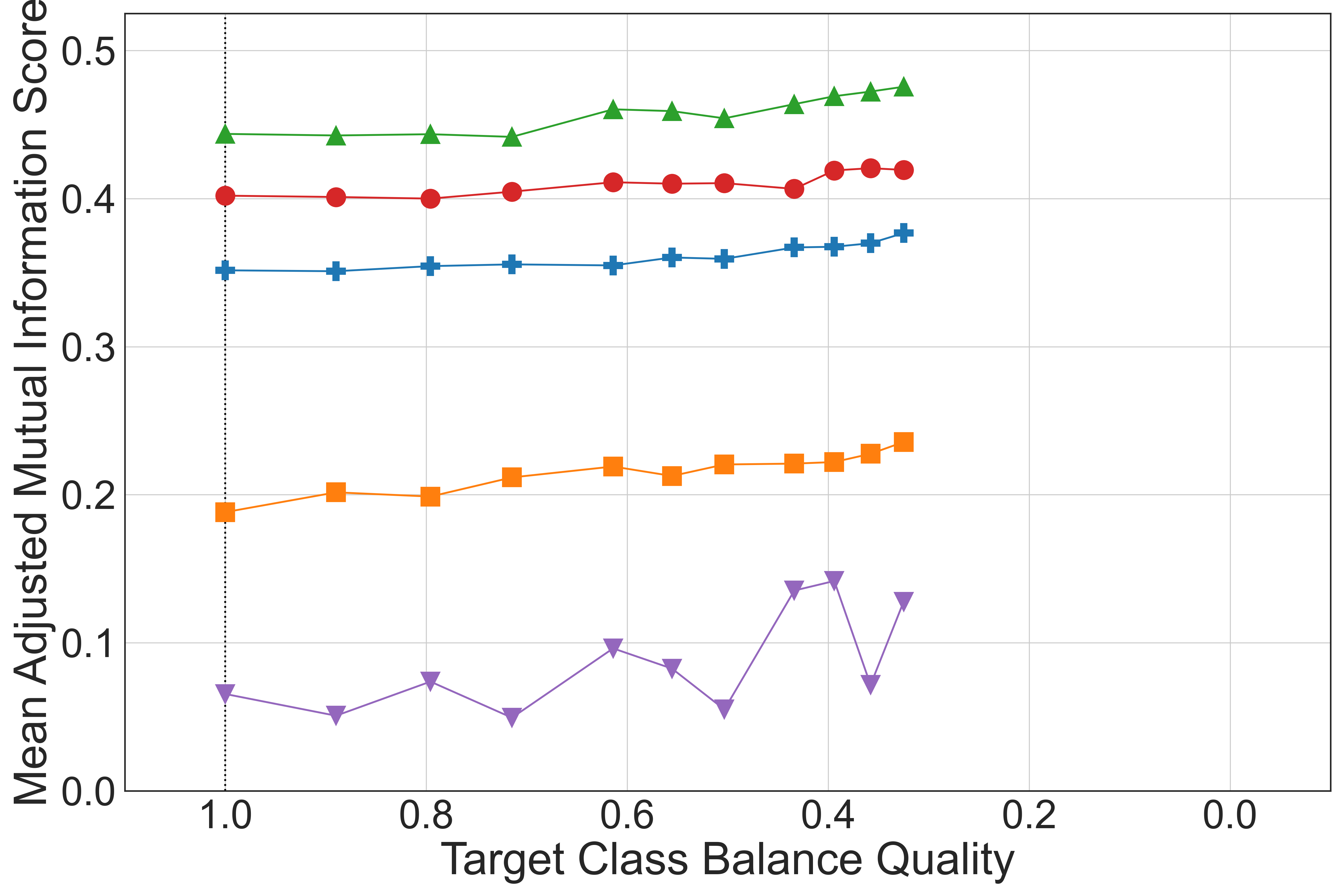
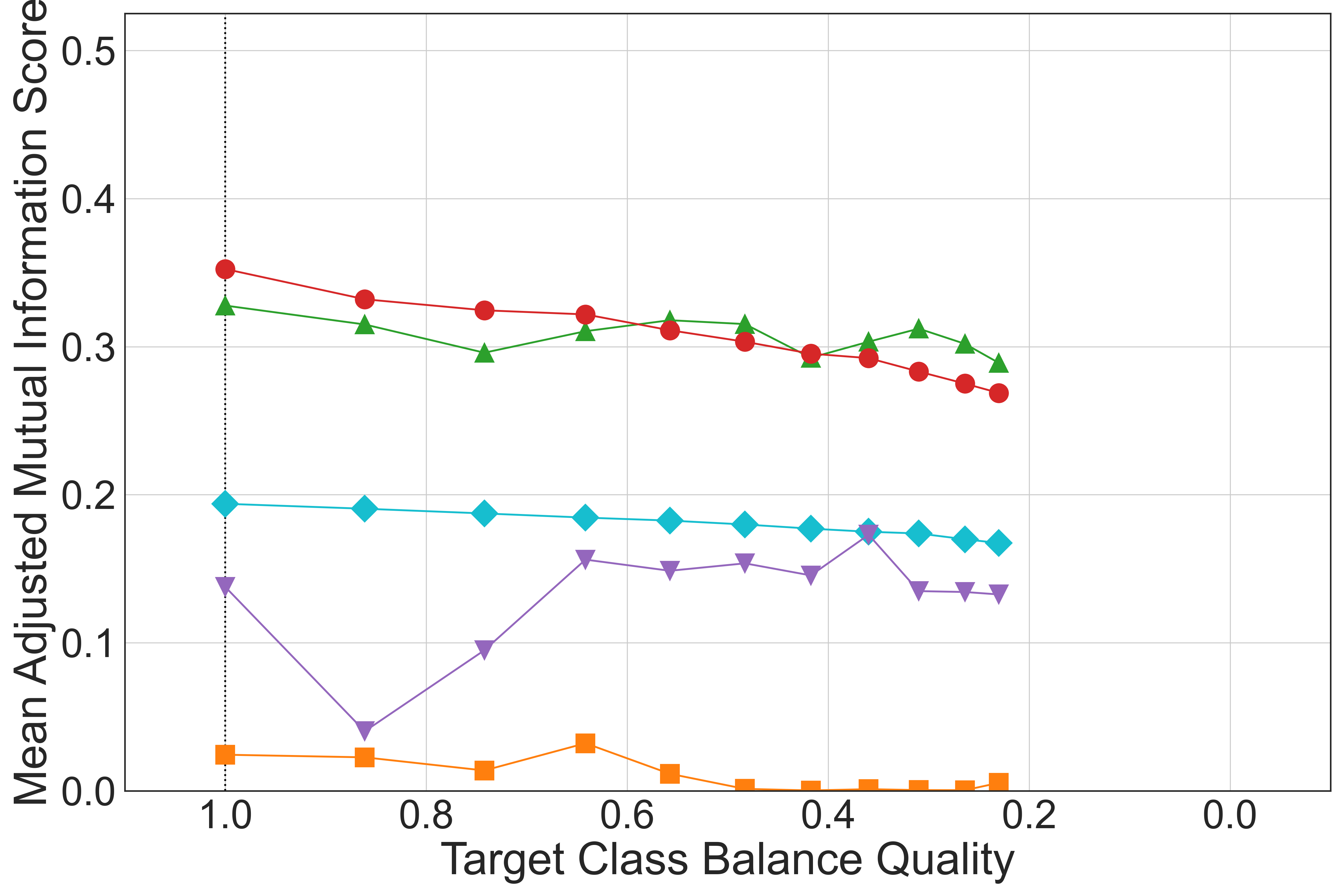

The pollution of the target accuracy should have no influence on any clustering algorithm, as they are unsupervised: a changed target class does not affect the clustering itself. However, the fact that we can still see a degrading curve in Figures 19(a), 19(c), and 19(b) is due to us comparing the clustering result with the polluted target classes and not with the original target classes when calculating AMI. An interesting observation is the slight but always existing increase in each algorithms’ performance for all three datasets at very low dataset qualities. We assume that a high pollution level changes enough target labels that, by chance, enough of the same labels are again changed to the same label, recreating parts of their original clusters. This effect is more noticeable with datasets that have fewer classes (i.e., Bank and Covertype) in their ground truth dataset, which strengthens our assumption.
Uniqueness.
We used the polluter that inserts duplicates based on a normal distribution. The Gaussian Mixture, k-Means / k-Prototypes and Agglomerative clustering algorithms are not affected by the pollution on Letter and Covertype as shown in Figures 21(a) and 21(b). Furthermore, the increase in duplicates helps the OPTICS approach to improve its performance: as a density-based clustering algorithm, it can benefit from somewhat evenly inserted duplicates as they increase the overall density of clusters and especially their cores without creating very dense cores consisting of only the same data point many times. The Autoencoder approach also enhances its performance above a certain number of duplicates for Letter. We assume that it is easier for the Autoencoder to learn the encoding if there are more duplicates in Letter. In contrast, we cannot see a clear behavior of the Autoencoder on Covertype, which is probably due to the additional time it would have needed to converge as well as the generally random and sample-dependent nature of neural network training. In Figure 21(c), we can see the clustering results of Bank with uniqueness pollution (see focused version in Appendix, Figure 26(f)). An important difference to all other polluters is that this one cleans the dataset before the actual pollution to create a baseline dataset with quality , removing all duplicates and thus strongly reducing Bank size, as it has many duplicated entries in its original state. On the one hand, we can see an improvement in performance for the k-Means and the Gaussian Mixture algorithms and a slight degradation in performance for the OPTICS algorithm with decreasing dataset quality. On the other hand, due to the strong dataset size reduction and the particularities of Bank mentioned at the beginning of Section 6.3, we should not put a lot of weight in these results, which lie in a much smaller AMI range than the other results, as a basis for conclusions and therefore refrain from further interpreting them.
Target Class Balance.
We observe a difference in behavior between Letter with numeric-only features and high-class count and Bank and Covertype with fewer classes and features. In Letter shown in Figure 20(a), the imbalance in cluster sizes actually slightly improved the AMI score. This behavior is approximately linear for all algorithms except for the Autoencoder-based clustering, which still improves over time but exhibits an irregular behavior while doing so. We believe that this irregularity is simply due to the neural network training step being highly dependent on the data given to it, which is changed as the class balance changes. We provide two causes for the slight increase in clustering quality as the target class balance degrades. For OPTICS, we found that the number of clusters being identified on average increased as the dataset grew more imbalanced (Figure 25(d) in Appendix), likely since clusters became denser for those classes which grew due to the imbalancing process. This is also the reason behind the improvement of other algorithms’ performance. As algorithms were never able to correctly identify all clusters, as evident by the AMI score being far from , the loss of information for some clusters may have been outweighed by the gain of information in other areas of the dataset, allowing algorithms to pick up on some clusters so much better, that it improved the overall clustering quality score. Additionally, we have to consider that smaller clusters also have less of an impact on the overall clustering quality, so their loss may not be reflected heavily in the overall adjusted mutual information score.
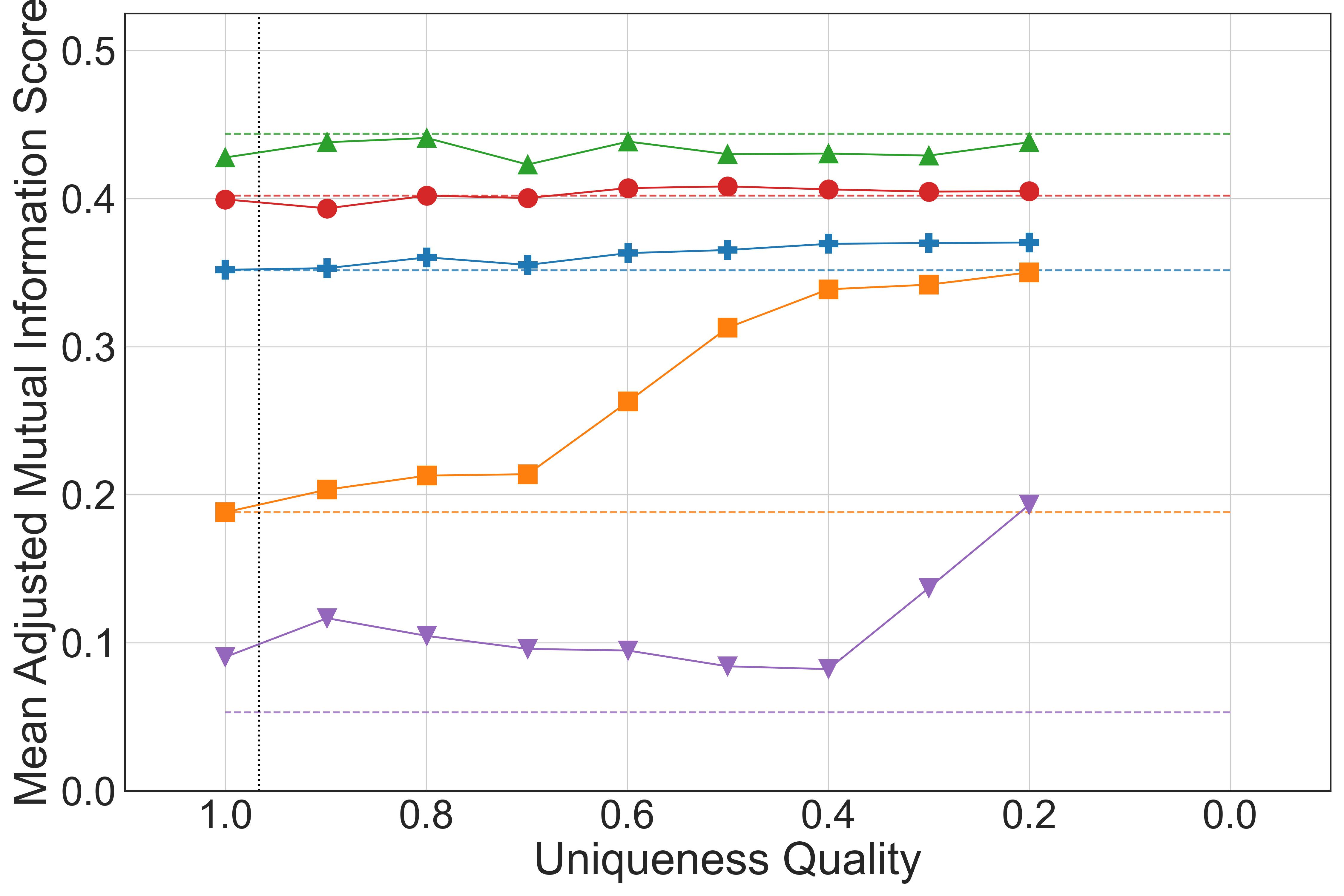
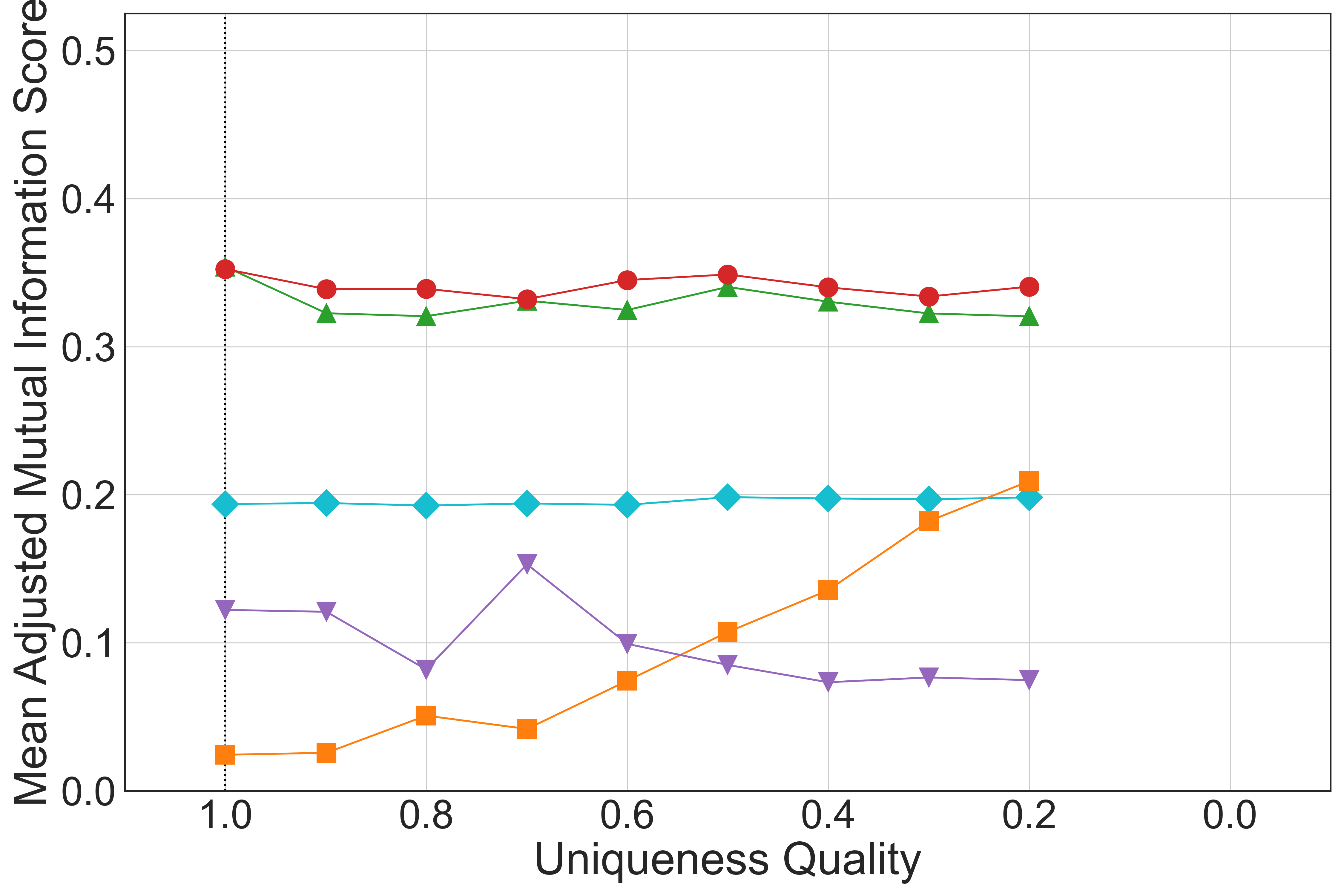
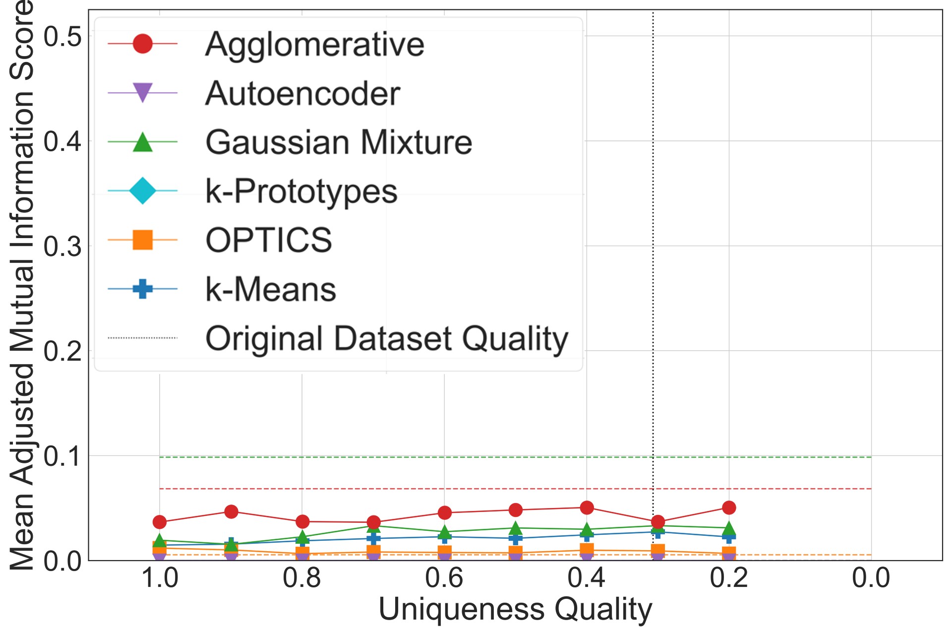
For Bank and Covertype (Figures 20(c) and 20(b)), we split the results analysis into three parts. First, we look at the k-Means / k-Prototypes and Agglomerative clustering algorithms. The k-Means / k-Prototypes algorithms’ AMI declines slightly and linearly, which can also be observed for the Agglomerative clustering on Covertype. This decline is caused by the inability of these algorithms to identify the shrunken clusters reliably, while they are also not majorly improving their recognition of the growing clusters. This may be the case in these datasets but not in Letter, as Covertype and Bank are harder to handle for the clustering algorithms in general, resulting in less improvement for the growing clusters. Additionally, there are fewer clusters overall to balance out or overtake the loss of quality coming with the difficulty to identify smaller clusters. The irregular behavior of the Agglomerative clustering on Bank hints at this algorithm’s instability on this particular dataset. We can see similar behavior when comparing it to the clustering results achieved when polluting the uniqueness quality dimension (Figure 21(c)), which strengthens our assumption of the Agglomerative clustering algorithm’s issues with this relatively small dataset with many repeating entries. Secondly, we analyze the OPTICS and Autoencoder clustering methods’ results. Here, we can see very differing behavior between the two datasets, with OPTICS and Autoencoder-based clustering performance being relatively constant in Bank (the Autoencoder has a score of 0 here), while they are experiencing drastic changes in quality for Covertype. However, we still group these together because for both datasets, the behavior of these algorithms matches the general behavior of the average number of clusters they were able to identify at each stage of pollution (Figures 25(f) and 25(e) in Appendix). We can observe that the AMI score decreases if the number of clusters identified by the Autoencoder or OPTICS algorithm decreases, with the AMI score being zero if only one cluster was identified. If the average number of clusters identified stays relatively constant, so does the algorithm performance, except a spike at a quality of about in Covertype for the Autoencoder clustering approach. The two algorithms can identify any number of clusters, however, the closer they get to identify the true number of clusters, the more likely they are to also truly identify groupings of data points in the dataset, even if these are only the cores of existing clusters. Just as hypothesized for the OPTICS algorithm on Letter, we believe that the change in number of clusters identified by these algorithms is rooted in the more or less dense regions in the polluted dataset when compared to the original data.
OPTICS struggles with improving in contrast to the Autoencoder, as it is more susceptible to the high dimensionality and presence of categorical features in Bank and Covertype after one-hot Encoding. The Gaussian Mixture clustering shows a different behavior in Bank and Covertype, however, in both cases it does not behave in a clear way due to the assumption of a specific distribution, as mentioned at the beginning of Section 6.3. Therefore, we believe that altering the samples in the dataset provided to the Gaussian Mixture clustering can have positive or negative effects, depending on whether this new sampling more or less resembles the assumed distribution of data.
7 Conclusion and future work
In this work, we experimentally studied the impact of six data quality dimensions on 15 algorithms from three ML tasks: classification, regression and clustering. We ran a vast number of experiments using quality degraded versions of nine real-world datasets. In addition, we distinguished between three scenarios that a data scientist could face while developing ML-pipelines: (1) polluted training set; (2) polluted test set; (3) polluted training and test sets. Table 2 shows a high-level view of our findings that we summarize along with recommendations in the following paragraphs.
|
Consistency |
Completeness |
F.-Accuracy |
T.-Accuracy |
Uniqueness |
Class Balance |
|
|---|---|---|---|---|---|---|
| Classification | ✓ | ✕ | ✕ | ✕ | ✓ | |
| Regression | ✓ | ✕ | ✕ | ✕ | ||
| Clustering | ✓ | ✕ | ✕ | ✓ | ✓ | ✓ |
Classification.
We found that the quality dimensions with the least impact are uniqueness, consistent representation and target class balance as long as the balance is not shifted towards a very extreme case. This suggests that with only a very low loss in classifier performance on tabular data, data scientists can skip pre-processing steps like exact de-duplication, unifying inconsistent representations, and carefully balancing the target variable.
For completeness, our findings suggest that missing values influence the performance of the classifiers the most if the classifier was not trained on data with missing values. The results also show that having less than 40% missing values in the training phase does not significantly decrease the model’s performance, which could be needed to increase robustness if no information is provided on how to impute the serving data once the model reaches production. Reducing the target accuracy of the training data results in degradation of model performance to below a majority classifier performance with target accuracy lower than . However, the results suggest that if 80% or more of data are labeled correctly, one can train classification models on that noisy data without significant loss in performance. Our insights also reinforce the importance of labeling test data carefully, as labeling errors could then lead to a significant underestimation of the model’s performance (e.g., with 40% label errors in Telco test data, the perceived performance of the classifier is below a baseline model).
A very low feature accuracy in the training data can also lead to a strong degradation of model performance, but similar to the target accuracy, there is a certain robustness to that, especially for linear models. Yet, the extent of this robustness is dataset-dependent. Reduced feature accuracy during serving time is also problematic but behaves more smoothly and in a linear trend, which makes performance estimation much easier if one can estimate the quality of the serving data. And even though the performance degrades constantly, it stays above baseline levels most of the time.
Regression.
We found that the quality dimensions with the largest impact are completeness, feature accuracy and target accuracy. A decrease of quality in one of those dimensions leads to a worse than linear decrease in algorithm performance. Furthermore, the presence of missing values or inaccurate features in the test data without training the ML algorithm on such kind of data leads to even worse performance. The dimensions uniqueness and target class balance show little impact. Still, we observed some degradation with small datasets and datasets with many features. We recommend not to focus on these two dimensions, when using large training datasets with a few features. Consistent representation has impact as soon as the new representations outweigh the old one.
For linear regression-based algorithms, ridge regression performs better or equal to linear regression because the regularization helps to cope better with polluted data. For tree-based algorithms, random forest always outperforms decision trees. The multi-layer perceptron’s performance highly depends on both the quality dimension and the dataset characteristics. Among all, random forest performs best across most cases, and thus seems to be the most robust algorithm. One exception is the target accuracy dimension. This insight coincides with the findings by aleryani2020multiple (2) investigating imputation methods for classification. They found ensemble learning the best performing approach for imputation when dealing with missing data.
Clustering.
We found the quality dimensions of completeness and feature accuracy to be the most impactful. In both cases, a degradation of the dataset quality led to a decrease in clustering performance, which was linear for datasets with categorical features and seemingly exponential concerning Letter containing only numerical features. The density-based OPTICS algorithm was most affected by changes in completeness and feature accuracy. The k-Means/k-Prototypes, Agglomerative clustering, and Gaussian Mixture clustering generally behaved similarly to one another. The Autoencoder approach was least affected by changes in these two quality dimensions.
An interesting observation is that Gaussian Mixture benefited from the slight noise added to numerical features in the first step of feature accuracy pollution. Therefore, we recommend using this approach when dealing with datasets containing exclusively numerical features if one suspects inaccuracies in their feature values. In case of mixed-type datasets, we can recommend only the k-Prototypes algorithm, as its degradation to initial performance trade-off performs the best in our experiments.
Surprisingly, the consistent representation, target accuracy, target class balance and uniqueness dimensions had very low impact on the performance of the majority of the examined algorithms. In contrast, adding some duplicate values into a completely duplicate-free dataset, decreasing its uniqueness, improved the performance of OPTICS significantly. We recommend refraining from using Agglomerative clustering when dealing with a dataset with inconsistent representations for its categorical features, as it was unable to deal with this kind of pollution. Overall, the k-Means/k-Prototypes algorithms, i.e., the centroid-based family, showed the most robustness regarding the six data quality dimensions. Nevertheless, the Agglomerative and Gaussian Mixture clustering algorithms outperformed the k-Means/k-Prototypes approaches on clean data. If you are aware that you are not dealing with a dataset containing both categorical and numerical features, where the features may take on erroneous values, we can also safely recommend the usage of the Gaussian Mixture clustering approach. While it does restrict usage to datasets that are approximately drawn from a mixture of Gaussian distributions, this approach generally performed better than most of the other clustering algorithms while being more resilient against data quality issues than the similarly well performing Agglomerative clustering algorithm.
Limitations and Future Work.
The lack of hyperparameter optimization in our work is intentional, as we are mainly interested in the impact of data quality on the algorithms’ performance; however, it also means that it is possible that the performance we reported is not the best for any algorithm. Another “hyperparameter” for the implementation of the completeness polluter is our choice of placeholder values. For each feature, a placeholder value is manually set, as described in Section 3.2. One downside of choosing one specific placeholder for each feature is the value set as placeholder, which could negatively influence the model performance. Comparing different values is a potential area for future work. This work could expand into the field of data imputation to evaluate which placeholder values reach the best model performance. In the clustering algorithms’ evaluation, we implemented the Autoencoder using a basic neural network, not yet optimized for its particular task. Improvements could include the usage of network components other than linear layers, or the incorporation of the clustering performance on the code space into the loss function. Additionally, we did not account for the information loss caused by encoding high-dimensional data into a two-dimensional embedded space.
In future work, it is important to use not only AMI to evaluate the clustering algorithm, but to also consider metrics such as absolute size of overlap of the original and generated data clustering and average and variance of the cluster sizes in the algorithm output. We also plan to expand our evaluation in two directions: adding more data quality dimensions and conducting a deeper evaluation per ML-model.
Acknowledgements.
This research was performed in the context of the KITQAR project, supported by Denkfabrik Digitale Arbeitsgemeinschaft im Bundesministerium für Arbeit und Soziales (BMAS).References
- (1) Aditya “100,000 UK Used Car Data Set” https://www.kaggle.com/adityadesai13/used-car-dataset-ford-and-mercedes/version/3, visited 2022-03-11
- (2) Aleryani, Wenjia Wang and Beatriz Iglesia “Multiple Imputation Ensembles (MIE) for Dealing with Missing Data” In SN Computer Science 1.3 Springer, 2020, pp. 1–20
- (3) Naomi S Altman “An introduction to kernel and nearest-neighbor nonparametric regression” In The American Statistician 46.3 Taylor & Francis Group, 1992, pp. 175–185
- (4) M. Ankerst, M. M. Breunig, H.-P. Kriegel and J. Sander “OPTICS: Ordering Points to Identify the Clustering Structure” In SIGMOD Record 28.2, 1999, pp. 49–60
- (5) Carlo Batini and Monica Scannapieco “Data Quality: Concepts, Methods and Techniques” Berlin – Heidelberg – New York: Springer Verlag, 2006
- (6) Felix Biessmann et al. “Automated Data Validation in Machine Learning Systems” In IEEE Data Engineering Bulletin 44.1, 2021, pp. 51–65
- (7) J. A. Blackard “Covertype Data Set” https://archive.ics.uci.edu/ml/datasets/Covertype, visited 2022-03-11
- (8) J. A. Blackard and D. J. Dean “Comparative Accuracies of Artificial Neural Networks and Discriminant Analysis in Predicting Forest Cover Types from Cartographic Variables” In Computers and Electronics in Agriculture 24.3 Elsevier, 1999, pp. 131–151
- (9) Eric Breck et al. “Data Validation for Machine Learning” In Proceedings of Machine Learning and Systems 2019, MLSys 2019 Stanford, CA, USA: mlsys.org, 2019
- (10) L. Breiman “Random forests” In Machine Learning 45.1 Springer, 2001, pp. 5–32
- (11) Leo Breiman, J. H. Friedman, R. A. Olshen and C. J. Stone “Classification and Regression Trees” Wadsworth, 1984
- (12) G. Chen, J. Vandenbulcke and E. E. Kerre “A General Treatment of Data Redundancy in a Fuzzy Relational Data Model” In Journal of the American Society for Information Science 43.4, 1992, pp. 304–311 URL: https://asistdl.onlinelibrary.wiley.com/doi/abs/10.1002/%28SICI%291097-4571%28199205%2943%3A4%3C304%3A%3AAID-ASI6%3E3.0.CO%3B2-X
- (13) P. Christen and K. Goiser “Quality and Complexity Measures for Data Linkage and Deduplication” In Quality Measures in Data Mining Springer, 2007, pp. 127–151
- (14) D. De Cock “Ames, Iowa: Alternative to the Boston Housing Data as an End of Semester Regression Project” In Journal of Statistics Education 19.3 Taylor & Francis, 2011, pp. null DOI: 10.1080/10691898.2011.11889627
- (15) NVIDIA Corporation “CUDA Toolkit” https://developer.nvidia.com/cuda-toolkit, visited 2022-03-11
- (16) Corinna Cortes and Vladimir Vapnik “Support-vector networks” In Machine learning 20.3 Springer, 1995, pp. 273–297
- (17) W. H. E. Day and H. Edelsbrunner “Efficient Algorithms for Agglomerative Hierarchical Clustering Methods” In Journal of Classification 1.1 Springer, 1984, pp. 7–24
- (18) Developers “OPTICS” https://scikit-learn.org/stable/modules/generated/sklearn.cluster.OPTICS.html, visited 2022-03-11
- (19) D. Dua and C. Graff “UCI Machine Learning Repository” http://archive.ics.uci.edu/ml, visited 2022-03-11, 2017
- (20) Martin Ester, Hans-Peter Kriegel, Jörg Sander and Xiaowei Xu “A Density-Based Algorithm for Discovering Clusters in Large Spatial Databases with Noise” In Proceedings of the International Conference on Knowledge discovery and data mining (SIGKDD) AAAI Press, 1996, pp. 226–231
- (21) Inc. Facebook “PyTorch: From Research to Production”, https://pytorch.org/
- (22) Matthias Feurer et al. “Efficient and Robust Automated Machine Learning” In Advances in Neural Information Processing Systems (NeurIPS), 2015, pp. 2962–2970
- (23) Daniele Foroni, Matteo Lissandrini and Yannis Velegrakis “Estimating the extent of the effects of Data Quality through Observations” In Proceedings of the International Conference on Data Engineering (ICDE), 2021, pp. 1913–1918 DOI: 10.1109/ICDE51399.2021.00176
- (24) Benoît Frénay and Michel Verleysen “Classification in the Presence of Label Noise: A Survey” In IEEE Trans. Neural Networks Learn. Syst. 25.5, 2014, pp. 845–869 DOI: 10.1109/TNNLS.2013.2292894
- (25) Timnit Gebru et al. “Datasheets for datasets” In Communications of the ACM 64.12, 2021, pp. 86–92 DOI: 10.1145/3458723
- (26) J. C. Gower “A General Coefficient of Similarity and Some of its Properties” In Biometrics 27.04 JSTOR, 1971, pp. 857–871
- (27) Christoph Gröger “There is No AI without Data” In Communications of the ACM 64.11 New York, NY, USA: Association for Computing Machinery, 2021, pp. 98–108 DOI: 10.1145/3448247
- (28) U. Grömping “South German Credit Data: Correcting a Widely Used Data Set”, 2019 URL: http://www1.beuth-hochschule.de/FB_II/reports/Report-2019-004.pdf
- (29) Venkat Gudivada, Amy Apon and Junhua Ding “Data quality considerations for big data and machine learning: Going beyond data cleaning and transformations” In International Journal on Advances in Software 10.1, 2017, pp. 1–20
- (30) Nitin Gupta et al. “Data Quality Toolkit: Automatic assessment of data quality and remediation for machine learning datasets” In CoRR abs/2108.05935, 2021 arXiv: https://arxiv.org/abs/2108.05935
- (31) D. Harrison and D. L. Rubinfeld “Hedonic Housing Prices and the Demand for Clean Air” In Journal of Environmental Economics and Management 5.1, 1978, pp. 81–102 DOI: https://doi.org/10.1016/0095-0696(78)90006-2
- (32) A. E. Hoerl and R. W. Kennard “Ridge Regression: Biased Estimation for Nonorthogonal Problems” In Technometrics 12.1 Taylor & Francis, 1970, pp. 55–67
- (33) Prof. H. Hofmann “Creditworthiness Dataset” https://archive.ics.uci.edu/ml/datasets/statlog+(german+credit+data), visited 2022-03-11
- (34) IBM “Telco Customer Churn Dataset” https://www.kaggle.com/blastchar/telco-customer-churn, visited 2022-03-11
- (35) I. F. Ilyas and X. Chu “Trends in Cleaning Relational Data: Consistency and Deduplication” In Foundations and Trends in Databases 5.4 Now Publishers Inc. Hanover, MA, USA, 2015, pp. 281–393
- (36) J. Ji et al. “An Improved k-Prototypes Clustering Algorithm for Mixed Numeric and Categorical Data” In Neurocomputing 120 Elsevier, 2013, pp. 590–596
- (37) Kaggle “House Prices - Advanced Regression Techniques” https://www.kaggle.com/c/house-prices-advanced-regression-techniques, visited 2022-03-11
- (38) Diederik P. Kingma and Jimmy Ba “Adam: A Method for Stochastic Optimization” In International Conference on Learning Representations (ICLR), 2015
- (39) Ch. N. S. Kumar, K. N. Rao, A. Govardhan and N. Sandhya “Subset k-Means Approach for Handling Imbalanced-distributed Data” In Emerging ICT for Bridging the Future-Proceedings of the Annual Convention of the Computer Society of India CSI Volume 2 Springer, 2015, pp. 497–508
- (40) M. Last, O. Maimon and E. Minkov “Improving Stability of Decision Trees” In International Journal of Pattern Recognition and Artificial Intelligence 16.02 World Scientific, 2002, pp. 145–159
- (41) Colin Lewis-Beck and Michael Lewis-Beck “Applied regression: An introduction” Sage publications, 2015
- (42) Peng Li et al. “CleanML: A Study for Evaluating the Impact of Data Cleaning on ML Classification Tasks” In Proceedings of the International Conference on Data Engineering (ICDE), 2021, pp. 13–24 URL: https://doi.org/10.1109/ICDE51399.2021.00009
- (43) T.-S. Lim “Contraceptive Method Choice Data Set”, 1987
- (44) R. J. A. Little and D. B. Rubin “Statistical Analysis with Missing Data” Wiley, 2014 DOI: 10.1002/9781119013563
- (45) S. Lu and R. Li “DAC–Deep Autoencoder-Based Clustering: A General Deep Learning Framework of Representation Learning” In Proceedings of SAI Intelligent Systems Conference Virtual Event: Springer, 2021, pp. 205–216
- (46) Peter McCullagh and John A. Nelder “Generalized Linear Models” Springer, 1989 DOI: 10.1007/978-1-4899-3242-6
- (47) D. C. Montgomery, E. A. Peck and G. G. Vining “Introduction to Linear Regression Analysis” John Wiley & Sons, 2021
- (48) S. Moro, P. Cortez and P. Rita “A Data-driven Approach to Predict the Success of Bank Telemarketing” In Decision Support Systems 62 Elsevier, 2014, pp. 22–31
- (49) Felix Neutatz et al. “Data Cleaning and AutoML: Would an Optimizer Choose to Clean?” In Datenbank Spektrum 22.2, 2022, pp. 121–130 DOI: 10.1007/s13222-022-00413-2
- (50) Felix Neutatz, Binger Chen, Ziawasch Abedjan and Eugene Wu “From Cleaning before ML to Cleaning for ML” In IEEE Data Eng. Bull. 44.1, 2021, pp. 24–41 URL: http://sites.computer.org/debull/A21mar/p24.pdf
- (51) Xuan Vinh Nguyen, Julien Epps and James Bailey “Information theoretic measures for clusterings comparison: is a correction for chance necessary?” In Proceedings of the International Conference on Machine Learning (ICML) 382, ACM International Conference Proceeding Series ACM, 2009, pp. 1073–1080 DOI: 10.1145/1553374.1553511
- (52) Curtis G. Northcutt, Anish Athalye and Jonas Mueller “Pervasive Label Errors in Test Sets Destabilize Machine Learning Benchmarks” In Proceedings of the Neural Information Processing Systems Track on Datasets and Benchmarks 1, NeurIPS Datasets and Benchmarks, 2021 URL: https://datasets-benchmarks-proceedings.neurips.cc/paper/2021/hash/f2217062e9a397a1dca429e7d70bc6ca-Abstract-round1.html
- (53) F. Pedregosa et al. “Scikit-learn: Machine Learning in Python” In Journal of Machine Learning Research 12, 2011, pp. 2825–2830
- (54) Neoklis Polyzotis, Sudip Roy, Steven Euijong Whang and Martin Zinkevich “Data Lifecycle Challenges in Production Machine Learning: A Survey” In SIGMOD Record 47.2, 2018, pp. 17–28 DOI: 10.1145/3299887.3299891
- (55) M. Ramadan “IMDb Most Popular Films and Series” https://www.kaggle.com/mazenramadan/imdb-most-popular-films-and-series/version/3, visited 2022-03-11
- (56) Cédric Renggli et al. “A Data Quality-Driven View of MLOps” In IEEE Data Engineering Bulletin 44.1, 2021, pp. 11–23 URL: http://sites.computer.org/debull/A21mar/p11.pdf
- (57) D. A. Reynolds “Gaussian Mixture Models” In Encyclopedia of Biometrics 741 Berlin, Springer, 2009, pp. 827–832
- (58) Lior Rokach and Oded Maimon “Clustering Methods” In The Data Mining and Knowledge Discovery Handbook Springer, 2005, pp. 321–352
- (59) Chris Ré “The Road to Software 2.0 or Data‑Centric AI”, 2021 URL: https://hazyresearch.stanford.edu/data-centric-ai
- (60) P. Cortez S. Moro and P. Rita “Bank Marketing Data Set” https://archive.ics.uci.edu/ml/datasets/bank+marketing, visited 2022-03-11
- (61) Sebastian Schelter, Tammo Rukat and Felix Biessmann “JENGA - A Framework to Study the Impact of Data Errors on the Predictions of Machine Learning Models” In Proceedings of the International Conference on Extending Database Technology (EDBT) OpenProceedings.org, 2021, pp. 529–534 DOI: 10.5441/002/edbt.2021.63
- (62) Sebastian Schelter, Tammo Rukat and Felix Bießmann “Learning to Validate the Predictions of Black Box Classifiers on Unseen Data” In Proceedings of the International Conference on Management of Data (SIGMOD) ACM, 2020, pp. 1289–1299 DOI: 10.1145/3318464.3380604
- (63) Sebastian Schelter et al. “Automating Large-Scale Data Quality Verification” In PVLDB 11.12, 2018, pp. 1781–1794 DOI: 10.14778/3229863.3229867
- (64) Sebastian Schelter et al. “On Challenges in Machine Learning Model Management” In IEEE Data Engineering Bulletin 41.4, 2018, pp. 5–15 URL: http://sites.computer.org/debull/A18dec/p5.pdf
- (65) K. P. Sinaga and M.-S. Yang “Unsupervised k-Means Clustering Algorithm” In IEEE access 8, 2020, pp. 80716–80727
- (66) D. J. Slate “Letter Recognition Dataset” https://archive.ics.uci.edu/ml/datasets/letter+recognition, visited 2022-03-11, 1991
- (67) C. Song et al. “Auto-encoder Based Data Clustering” In Iberoamerican Congress on Pattern Recognition Berlin, Heidelberg: Springer Berlin Heidelberg, 2013, pp. 117–124
- (68) D. Specht “A General Regression Neural Network” In IEEE Transactions on Neural Networks 2, 1991, pp. 568–578 DOI: 10.1109/72.97934
- (69) Julia Stoyanovich and Bill Howe “Nutritional Labels for Data and Models” In IEEE Data Engineering Bulletin 42.3, 2019, pp. 13–23 URL: http://sites.computer.org/debull/A19sept/p13.pdf
- (70) Jacopo Tagliabue, Ville Tuulos, Ciro Greco and Valay Dave “DAG Card is the new Model Card” In CoRR abs/2110.13601, 2021, pp. 1–6 arXiv: https://arxiv.org/abs/2110.13601
- (71) N. X. Vinh, J. Epps and J. Bailey “Information Theoretic Measures for Clusterings Comparison: Variants, Properties, Normalization and Correction for Chance” In The Journal of Machine Learning Research 11 JMLR. org, 2010, pp. 2837–2854
- (72) R. Y. Wang and D. M. Strong “Beyond Accuracy: What Data Quality Means to Data Consumers” In J. Manag. Inf. Syst. 12.4, 1996, pp. 5–33 URL: http://www.jmis-web.org/articles/1002
The Appendix provides some additional plots from the conducted experiments that were discussed in the report, but moved to the appendix to improve the readability of the report.
We show in Figure 23, the performance of the classification algorithms when we decrease the data consistency with . The same for clustering algorithm is shown in Figure 24. We also included in Figure 25 the plots from the regression experiments where the uniqueness polluter added duplicates following a normal distribution.
For better understanding some clustering results, it is beneficial to see the correlation between the number of clusters identified by the OPTICS and Autoencoder clustering approaches to their performance. Please note that the Agglomerative and k-Means / k-Prototypes algorithms are always returning the expected number of clusters as this is one of their input parameters. The Gaussian Mixtures algorithm is also coerced to do this; however, it is not guaranteed to return the correct number of clusters. Therefore, these three lines commonly overlap and only one of them is visible in the plots. The number of clusters shown in Figure 26 is averaged over the 5 different runs of each algorithm on a given dataset, and can therefore also take on floating-point values.
Finally, as the line plots shown in the clustering result chapter (see Section 6.3) for the Bank dataset are difficult to read because of the shared y-axis among the different datasets, we decided to also add a focused version of these plots in Figure 27.