Two-dimensional spectroscopic diagnosis of quantum coherence in Fermi polarons

Abstract

We present a full microscopic many-body calculation of a recently-proposed nonlinear two-dimensional spectroscopy for Fermi polarons, and show that the quantum coherence between the attractive and repulsive polarons, which has never been experimentally examined, can be unambiguously revealed via quantum beats at the two off-diagonal crosspeaks in the two-dimensional spectrum. We predict that particle-hole excitations make the two crosspeaks asymmetric and lead to an additional side peak near the diagonal repulsive polaron peak. Our simulated spectra can be readily examined in future cold-atom experiments, where the two-dimensional spectroscopy is to be implemented by using a Ramsey interference sequence of rf pulses in the time domain. Our results also provide a first-principle understanding of the recent two-dimensional coherent spectroscopy of interacting excitons and trions in doped monolayer transition metal dichalcogenides.

The polaron physics that describes the dynamics of a single impurity interacting with a many-body environment is a long-standing problem in modern physics Alexandrov2010 . The early study in 1933 by Lev Landua Landau1933 led to the cornerstone concept of quasiparticles, which vividly characterizes the ability of the impurity operating in its own, free-particle-like way in terms of a residue $0<Z<1$. Over the next 70 years, sequent studies of the polaron problem generated a number of celebrated ideas in many-body physics and condensed matter physics, such as Kondo screening Hewson1993 , Anderson’s orthogonality catastrophe Anderson1967 , the x-ray Fermi edge singularity Mahan1967 ; Roulet1969 ; Nozieres1969 , Nagaoka ferromagnetism Nagaoka1966 ; Shastry1990 ; Basile1990 and the phase string effect Sheng1996 .

Over the past two decades, the polaron physics has received much more intense interests, owing to the unprecedented controllability achieved in ultracold atomic gases Bloch2008 ; Chin2010 . The dynamics of an impurity atom immersed in a Fermi sea (Fermi polaron) Schirotzek2009 ; Zhang2012 ; Kohstall2012 ; Koschorreck2012 ; Cetina2016 ; Scazza2017 or in a weakly interacting Bose condensate (Bose polaron) Hu2016 ; Jorgensen2016 has now been systematically investigated in a quantitative manner Massignan2014 ; Lan2014 ; Schmidt2018 , with precisely tunable masses and interactions. 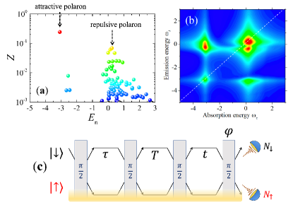A remarkable discovery in this context is the observation of repulsive polaron Kohstall2012 ; Koschorreck2012 ; Scazza2017 ; Cui2010 ; Massignan2011 , which is a collection of excited many-body states with non-negligible residues close to a characteristic energy (i.e., repulsive polaron energy), as illustrated in Fig. 1(a). The repulsive polaron separates from the ground-state attractive polaron by a spectral gap (i.e., dark continuum Goulko2016 ; Wang2022PRL ; Wang2022PRA ) and can be quantitatively characterized in experiments by using injected radio-frequency (rf) spectroscopy Scazza2017 . As an excited quasiparticle, repulsive polaron is naturally anticipated to coherently couple to attractive polaron, in the same way as an effective two-level quantum system. Unfortunately, such a quantum coherence has never been experimentally verified in cold-atom laboratories, by using either Rabi-type or Ramsey-type interferometry Cetina2016 ; Schmidt2018 ; Knap2012 .

Figure 1: (a) An example of the residues at different many-body polaron states. The ground-state attractive polaron and the excited repulsive polaron at the energy $E_{A}$ and $E_{R}$ have been explicitly indicated. (b) A typical 2DS spectrum of Fermi polarons at the mixing time $T=0$, where the absorption energy ($\omega_{\tau}$) and emission energy ($\omega_{t}$) are obtained by Fourier transforming the time delays $\tau$ and $t$, respectively. Two asymmetric crosspeaks at $(\omega_{\tau},\omega_{t})=(E_{A},E_{R})$ and $(E_{R},E_{A})$, off the diagonal direction (i.e., the dotted line), reveal the coherence between the attractive and repulsive polarons. (c) The 2DS pulse sequence in the time domain, defined by the time delays ($\tau,T,t$). The impurity in the spin-up state interacts with a background Fermi sea, as indicated by the shaded area.

The purpose of this Letter is to present quantitative, experimentally testable predictions on a novel nonlinear two-dimensional spectroscopy (2DS) of Fermi polarons, which can provide an unambiguous spectroscopic diagnosis of the quantum coherence between attractive and repulsive polarons via quantum beats at two off-diagonal crosspeaks in the 2DS spectrum, as shown in Fig. 1(b). This 2DS - implemented by a sequence of Ramsey-type $\pi/2$ rf pulses as given in Fig. 1(c) - was recently proposed by one of us in Ref. Wang2022PRX , where exact quantum dynamics in the presence of an infinitely heavy impurity has been considered. However, the immobile, heavy polaron limit suffers from Anderson’s orthogonality catastrophe that renders Fermi polaron quasiparticles into power-law singularities Anderson1967 ; Knap2012 . Thus, strictly speaking, it can only provide a qualitative understanding for the 2DS of Ferm polarons. Here, such a difficulty is overcome by a microscopic many-body calculation for a mobile impurity with finite mass. As a consequence, we are able to analytically clarify that the Fermi sea shaking Schmidt2018 ; Knap2012 , in the form of particle-hole excitations, makes the 2DS highly asymmetric. We find that the Fermi sea shaking also introduces an interesting side peak in the 2DS, slightly below the diagonal peak at the repulsive polaron energy.

It is worth noting that the 2DS is a cold-atom analogue of the well-known two-dimensional coherent spectroscopy (2DCS) in condensed matter physics Jonas2003 ; Li2006 ; Cho2008 ; Davis2008 ; Nardin2015 . The latter has been widely used to reveal the many-body dynamics in semiconductors Li2006 ; Nardin2015 ; Dey2016 ; Hao2016NatPhys ; Hao2016NanoLett , although its full potential is severely limited by the lack of theoretical interpretation at the microscopic level Li2006 ; Tempelaar2019 ; Reichman2002 . Interacting excitons and trions in doped monolayer transition metal dichalcogenides (TMD) are intriguing examples Hao2016NanoLett ; Tempelaar2019 ; Muir2022 ; Reichman2002 . Remarkably, such systems have recently been understood as Fermi polarons Sidler2017 ; Efimkin2017 , where excitons and trions can be precisely re-interpreted as repulsive and attractive polarons, respectively. Despite the different excitation schemes (i.e., the spin flip by rf pulses in 2DS versus the exciton creation and annihilation by lasers in 2DCS), we find that our simulated spectra provide an excellent explanation to the experimental 2DCS of excitons and trions Hao2016NanoLett . Our results therefore present an exciting representative case, towards a full ab initio understanding of the 2DCS in condensed matter.

Model. The system under consideration consists of a single spin-1/2 impurity (with creation operator $d_{\mathbf{k}\sigma}^{\dagger}$ for two hyperfine states $\sigma=\uparrow,\downarrow$) immersed in a non-interacting Fermi bath (with creation operator $c_{\mathbf{k}}^{\dagger}$), as described by the model Hamiltonian ($\hbar=1$),

$$\mathcal{H}_{\sigma}=\sum_{\mathbf{k}}\left[\epsilon_{\mathbf{k}}c_{\mathbf{k}}^{\dagger}c_{\mathbf{k}}+\left(\epsilon_{\mathbf{k}}^{I}+\omega_{s}\delta_{\sigma\uparrow}\right)d_{\mathbf{k}\sigma}^{\dagger}d_{\mathbf{k}\sigma}\right]+\mathcal{H}_{U}\delta_{\sigma\uparrow},$$ (1)

when the impurity is the spin-$\sigma$ state. Here, $\epsilon_{\mathbf{k}}$ and $\epsilon_{\mathbf{k}}^{I}$ are respectively the kinetic energies of the bath and impurity, $\omega_{s}$ denotes the energy difference between the two spin states and is typically much larger than all other energy scales in the problem, and $\delta_{\sigma\sigma^{\prime}}$ is the usual Kronecker delta. The spin-up state of the impurity is tuned by Feshbach resonance Chin2010 to be strongly interacting with the Fermi bath, as described by the contact interaction Hamiltonian $\mathcal{H}_{U}=U\sum_{\mathbf{qkp}}d_{\mathbf{k\uparrow}}^{\dagger}c_{\mathbf{q-k}}^{\dagger}c_{\mathbf{q}-\mathbf{p}}d_{\mathbf{p}\uparrow}$. This gives rise to the many-body polaron states, as sketched in Fig. 1(a). In contrast, the spin-down impurity state has negligible interaction with the bath.

Theory of 2DS. In the standard Ramsey interferometry Cetina2016 ; Knap2012 , which involves only the first and the final $\pi/2$ rf pulses in Fig. 1(c), the spin-down impurity state acts a reference for phase evolution. The first pulse turns the initially prepared spin-down state $\left|\downarrow\right\rangle$ into a superposition $(\left|\uparrow\right\rangle+\left|\downarrow\right\rangle)/\sqrt{2}$, in which during the later evolution the spin-up state $\left|\uparrow\right\rangle$ acquires an additional phase due to the interaction with the Fermi bath. This phase difference can be read out by applying the final detection $\pi/2$ rf pulse and measuring the two occupation numbers $N_{\uparrow}$ and $N_{\downarrow}$ Cetina2016 ; Knap2012 . The resulting Ramsey response, given by the quantum average of the Pauli matrix $\left\langle\sigma_{x}\right\rangle$, can reveal the existence of both attractive and repulsive polarons Wang2022PRL ; Wang2022PRA ; Knap2012 . In our 2DS measurement Wang2022PRX , two more $\pi/2$ rf pulses are utilized to explore the many-body evolution in the multidimensional time domain and hence unfold quantum correlations between the two polaron branches.

To show this, let us express the $\pi/2$ rf pulse in terms of the operators $\hat{n}=\sum_{\mathbf{k}\sigma}d_{\mathbf{k}\sigma}^{\dagger}d_{\mathbf{k}\sigma}$ and $\hat{s}_{+}=\sum_{\mathbf{k}}d_{\mathbf{k}\uparrow}^{\dagger}d_{\mathbf{k}\downarrow}$, i.e., $R_{\pi/2}=(\hat{n}+\hat{s}_{+}-\hat{s}_{-})/\sqrt{2}$, where $\hat{s}_{-}\equiv\hat{s}_{+}^{\dagger}$. The time evolution between two pulses is given by $\mathcal{U}(t^{\prime})=e^{-i\mathcal{H}t^{\prime}}$ for $t^{\prime}=\tau,T,t$ and $\mathcal{H}$ can be either $\mathcal{H}_{\uparrow}$ or $\mathcal{H}_{\downarrow}$ depending on the impurity state during time evolution. Denoting the initial many-body state as $\left|\psi_{i}\right\rangle=d_{\mathbf{K}\downarrow}^{\dagger}\left|\textrm{FS}\right\rangle$, where $\left|\textrm{FS}\right\rangle$ describes the Fermi sea at zero temperature filled by particles with momentum $\left|\mathbf{k}\right|<k_{F}$ and the impurity is assumed to have a definite initial momentum $\mathbf{K}$, the final state $\left|\psi_{f}\right\rangle$ before the last detection pulse can be written as,

$$\left|\psi_{f}\right\rangle=\mathcal{U}\left(t\right)R_{\pi/2}\mathcal{U}\left(T\right)R_{\pi/2}\mathcal{U}\left(\tau\right)\frac{d_{\mathbf{K}\uparrow}^{\dagger}+d_{\mathbf{K}\downarrow}^{\dagger}}{\sqrt{2}}\otimes\left|\textrm{FS}\right\rangle.$$

The measurement of the Pauli matrix $\sigma_{+}=\sigma_{x}+i\sigma_{y}=2\hat{s}_{+}$ at the detection stage then yields the 2DS response Wang2022PRX , $\tilde{S}(\tau,T,t)=-2\left\langle\psi_{f}\left|\hat{s}_{+}\right|\psi_{f}\right\rangle$.

By inserting the expression of $R_{\pi/2}$ into $\left|\psi_{f}\right\rangle$, it is straightforward to check that $\tilde{S}(\tau,T,t)$ has sixteen different combinations Wang2022PRX , each of which corresponds to a pathway connecting the six unitary evolution operators $\mathcal{U}$ and has a different phase associated with the largest energy scale $\omega_{s}$. As the rf pulse is in principle tuned in resonant with $\omega_{s}$, we can take the rotating wave approximation and consider only two dominant pathways Wang2022PRX , $I_{i}(\tau,T,t)=\left\langle\textrm{FS}\right|d_{\mathbf{K}\downarrow}\hat{I}_{i}d_{\mathbf{K}\uparrow}^{\dagger}\left|\textrm{FS}\right\rangle$, where

$$\hat{I}_{1} \equiv e^{i\mathcal{H}_{\downarrow}\tau}\hat{s}_{-}e^{i\mathcal{H}_{\uparrow}T}\hat{n}e^{i\mathcal{H}_{\uparrow}t}\hat{s}_{+}e^{-i\mathcal{H}_{\downarrow}t}\hat{s}_{-}e^{-i\mathcal{H}_{\uparrow}T}\hat{n}e^{-i\mathcal{H}_{\uparrow}\tau},$$

$$\hat{I}_{2} \equiv e^{i\mathcal{H}_{\downarrow}\tau}\hat{n}e^{i\mathcal{H}_{\downarrow}T}\hat{s}_{-}e^{i\mathcal{H}_{\uparrow}t}\hat{s}_{+}e^{-i\mathcal{H}_{\downarrow}t}\hat{n}e^{-i\mathcal{H}_{\downarrow}T}\hat{s}_{-}e^{-i\mathcal{H}_{\uparrow}\tau}.$$

There are also two pathways $I_{3}$ and $I_{4}$ that are of marginal importance due to their fast-oscillating phase factor $e^{\pm i\omega_{s}T}$ at nonzero mixing time $T$ Wang2022PRX . However, they can easily be eliminated by a phase cycling procedure Wang2022PRX , i.e., by considering another Ramsey sequence, in which after the $\tau$-delay we take a $-\pi/2$ rf pulse instead of a $+\pi/2$ pulse. By denoting the corresponding response as $\tilde{S}_{-}(\tau,T,t)$, we define the phase cycling 2DS response that is of central interest Wang2022PRX ,

$$\mathcal{S}\left(\tau,T,t\right)=\tilde{S}-\tilde{S}_{-}=\frac{I_{1}\left(\tau,T,t\right)+I_{2}\left(\tau,T,t\right)}{2}.$$ (2)

In general, $I_{i}(\tau,T,t)$ ($i=1,2$) are extremely difficult to calculate for an interacting many-body system. Nevertheless, for Fermi polarons we can obtain the analytic expressions of $I_{i}(\tau,T,t)$, by taking the advantage that any ($n$-th) polaron state can be exactly expressed through multiple-particle-hole excitations of the Fermi sea Shastry1990 ; Basile1990 ; Chevy2006 ,

$$\left|n;\mathbf{k}\right\rangle =\sum_{\vec{\kappa}_{\nu}}\phi_{\vec{\kappa}_{\nu}}^{(n)}\left(\mathbf{k}\right)d_{\mathbf{k}-\mathbf{k}_{\vec{\kappa}_{\nu}}\uparrow}^{\dagger}\left|\vec{\kappa}_{\nu}\right\rangle,$$

where $\left|\vec{\kappa}_{\nu}\right\rangle=\prod_{i=1}^{\nu}c_{\mathbf{k}_{p}^{(i)}}^{\dagger}\prod_{i=1}^{\nu}c_{\mathbf{k}_{h}^{(i)}}\left|\textrm{FS}\right\rangle$ denotes $\nu$ particle-hole pairs excitations on top of a Fermi sea, $\vec{\kappa}_{\nu}\equiv\{\mathbf{k}_{p}^{(1)},\mathbf{k}_{p}^{(2)},\cdots,\mathbf{k}_{p}^{(\nu)};\mathbf{k}_{h}^{(1)},\mathbf{k}_{h}^{(2)},\cdots,\mathbf{k}_{h}^{(\nu)}\}$ is a collective notation for the $\nu$ particle momenta ($\mathbf{k}_{p}^{(i)}>k_{F}$) and hole momenta ($\mathbf{k}_{h}^{(i)}<k_{F}$), and therefore the total momentum and energy of the particle-hole excitations are given by $\mathbf{k}_{\vec{\kappa}_{\nu}}\equiv\sum_{i=1}^{\nu}[\mathbf{k}_{p}^{(i)}-\mathbf{k}_{h}^{(i)}]$ and $\epsilon_{\vec{\kappa}_{\nu}}=\sum_{i=1}^{\nu}[\epsilon_{\mathbf{k}_{p}^{(i)}}-\epsilon_{\mathbf{k}_{h}^{(i)}}]$, respectively. At the leading order without particle-hole excitations, we simply have $\left|\vec{\kappa}_{\nu=0}\right\rangle=\left|\textrm{FS}\right\rangle$ and $\phi_{\vec{\kappa}_{\nu=0}}^{(n)}(\mathbf{k})=\phi_{0}^{(n)}(\mathbf{k}).$ The energy of the ($n$-th) polaron state can be denoted as, $\mathcal{E}_{n}(\mathbf{k})=E_{\uparrow}^{(n)}(\mathbf{k})-(\epsilon_{\mathbf{k}}^{I}+\omega_{s}+E_{\textrm{FS}})$, after the subtraction of the impurity energy ($\epsilon_{\mathbf{k}}^{I}+\omega_{s}$) and the energy of the background Fermi sea ($E_{\text{FS}}$). On the other hand, the many-body eigenstates in the case of the spin-down impurity are much simpler and can be directly characterized by $\vec{\kappa}_{\nu}$, i.e., $\left|\vec{\kappa}_{\nu};\mathbf{k}\right\rangle=d_{\mathbf{k}-\mathbf{k}_{\vec{\kappa}_{\nu}}\downarrow}^{\dagger}\left|\vec{\kappa}_{\nu}\right\rangle$. The corresponding energy is given by, $\delta\mathcal{E}_{\vec{\kappa}_{\nu}}(\mathbf{k})=E_{\downarrow}^{(\vec{\kappa}_{\nu})}(\mathbf{k})-(\epsilon_{\mathbf{k}}^{I}+E_{\textrm{FS}})=\epsilon_{\vec{\kappa}_{\nu}}+\epsilon_{\mathbf{\mathbf{k}-\mathbf{k}_{\vec{\kappa}_{\nu}}}}^{I}-\epsilon_{\mathbf{k}}^{I}$, which is a summation of recoil energy of the impurity and the Fermi sea.

Let us now formally expand the time evolution operators as ($t^{\prime}=\tau,T,t$),

$$e^{\pm i\mathcal{H}_{\uparrow}t^{\prime}} = \sum_{n\mathbf{k}}e^{\pm iE_{\uparrow}^{(n)}(\mathbf{k})t^{\prime}}\left|n;\mathbf{k}\right\rangle\left\langle n;\mathbf{k}\right|,$$

$$e^{\pm i\mathcal{H}_{\downarrow}t^{\prime}} = \sum_{\vec{\kappa}_{\nu}\mathbf{k}}e^{\pm iE_{\downarrow}^{(\vec{\kappa}_{\nu})}(\mathbf{k})t^{\prime}}\left|\vec{\kappa}_{\nu};\mathbf{k}\right\rangle\left\langle\vec{\kappa}_{\nu};\mathbf{k}\right|,$$

and insert them into the expression of $I_{i}(\tau,T,t)$ ($i=1,2$). By using the identities, such as $\left\langle n;\mathbf{q}\right|d_{\mathbf{k}\uparrow}^{\dagger}\left|\textrm{FS}\right\rangle=\phi_{0}^{(n)*}(\mathbf{k})\delta_{\mathbf{kq}}$ and $\left\langle\vec{\kappa}_{\nu};\mathbf{k}\right|\hat{s}_{-}\left|n;\mathbf{q}\right\rangle=\phi_{\vec{\kappa}_{\nu}}^{(n)}(\mathbf{k})\delta_{\mathbf{kq}}$, after some straightforward algebra we find that,

$$I_{1} = \sum_{nm\vec{\kappa}_{\nu}}\Phi_{\vec{\kappa}_{\nu}}^{(nm)}e^{-i\mathcal{E}_{n}\tau}e^{-i\left(\mathcal{E}_{n}-\mathcal{E}_{m}\right)T}e^{i\left(\mathcal{E}_{m}-\delta\mathcal{E}_{\vec{\kappa}_{\nu}}\right)t},$$

$$I_{2} = \sum_{nm\vec{\kappa}_{\nu}}\Phi_{\vec{\kappa}_{\nu}}^{(nm)}e^{-i\mathcal{E}_{n}\tau}e^{-i\delta\mathcal{E}_{\vec{\kappa}_{\nu}}T}e^{i\left(\mathcal{E}_{m}-\delta\mathcal{E}_{\vec{\kappa}_{\nu}}\right)t},$$

where $\Phi_{\vec{\kappa}_{\nu}}^{(nm)}\equiv\phi_{0}^{(n)*}\phi_{0}^{(m)}\phi_{\vec{\kappa}_{\nu}}^{(n)}\phi_{\vec{\kappa}_{\nu}}^{(m)*}$ and we have omitted the dependence on the polaron momentum $\mathbf{K}$, i.e., $\phi_{\vec{\kappa}_{\nu}}^{(n)}(\mathbf{K})\equiv\phi_{\vec{\kappa}_{\nu}}^{(n)}$, $\mathcal{E}_{n}\left(\mathbf{K}\right)\equiv\mathcal{E}_{n}$ and $\delta\mathcal{E}_{\vec{\kappa}_{\nu}}(\mathbf{K})\equiv\delta\mathcal{E}_{\vec{\kappa}_{\nu}}$. By further taking a double Fourier transformation Wang2022PRX ; Jonas2003 ; Nardin2015 $\mathcal{A}(\omega_{\tau},T,\omega_{t})=\iintop_{0}^{\infty}d\tau dte^{i(\omega_{\tau}+\omega_{s})\tau}\tilde{S}(\tau,T,t)e^{-i(\omega_{t}+\omega_{s})t}/\pi^{2}$, we eventually arrive at,

$$\mathcal{A}=\frac{1}{2\pi^{2}}\sum_{nm\vec{\kappa}_{\nu}}\frac{\Phi_{\vec{\kappa}_{\nu}}^{(nm)}}{\omega_{\tau}^{+}-\mathcal{E}_{n}}\frac{\left[e^{-i\left(\mathcal{E}_{n}-\mathcal{E}_{m}\right)T}+e^{-i\delta\mathcal{E}_{\vec{\kappa}_{\nu}}T}\right]}{\omega_{t}^{-}-\mathcal{E}_{m}+\delta\mathcal{E}_{\vec{\kappa}_{\nu}}},$$ (3)

where $\omega_{\tau}^{+}\equiv\omega_{\tau}+i0^{+}$ and $\omega_{t}^{-}\equiv\omega_{t}-i0^{+}$, due to their absorption and emission characteristic, respectively. This exact analytic expression of the 2DS of Fermi polaron is the main result of this Letter. We aslo emphasize that our expression of MDS can be easily generalized to Bose polaron by replacing the multiple particle-hole excitations with Bogoliubov excitations accordingly. A derivation of the 1DS using the same approach is given in the Supplemental Material SM .

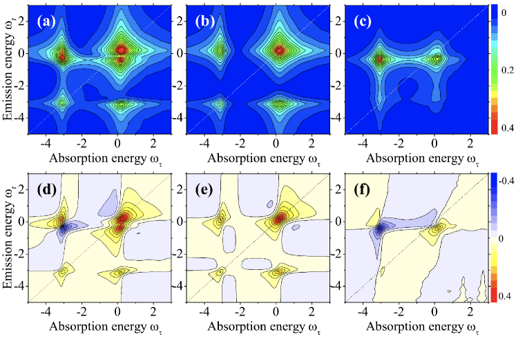
Figure 2: Upper panel: The amplitude of the 2DS spectrum, $\left|\mathcal{A}(\omega_{\tau},T=0,\omega_{t})\right|$ (a), and its symmetric and asymmetric components, $\left|\mathcal{A}_{s}(\omega_{\tau},T=0,\omega_{t})\right|$ (b) and $\left|\mathcal{A}_{a}(\omega_{\tau},T=0,\omega_{t})\right|$ (c). Lower panel: The corresponding real part of the 2DS spectrum, $\textrm{Re}\mathcal{A}(\omega_{\tau},T=0,\omega_{t})$ (d), $\textrm{Re}\mathcal{A}_{s}(\omega_{\tau},T=0,\omega_{t})$ (e) and $\textrm{Re}\mathcal{A}_{a}(\omega_{\tau},T=0,\omega_{t})$ (f). $\omega_{\tau}$ and $\omega_{t}$ are in units of the hopping strength $t_{c}$, and $A(\omega_{\tau},T,\omega_{t})$ is in units of $t_{c}^{-2}$.

To analyze the 2D Ramsey response, it is illustrative to truncate to one-particle-hole excitations (i.e., the so-called Chevy ansatz Chevy2006 ; Cetina2016 ; Parish2016 ), which is known to yield quantitatively accurate attractive polaron energy Massignan2014 . By explicitly listing the particle momentum ($\mathbf{k}_{p}$) and hole momentum ($\mathbf{k}_{h}$) in $\vec{\kappa}_{\nu=1}$ and denoting $\mathcal{\delta E}_{\vec{\kappa}_{\nu=1}}=\delta\mathcal{E}_{\mathbf{k}_{p}\mathbf{k}_{h}}=\epsilon_{\mathbf{k}_{p}}-\epsilon_{\mathbf{k}_{h}}+\epsilon_{\mathbf{K-}\mathbf{k}_{p}+\mathbf{k}_{h}}^{I}-\epsilon_{\mathbf{K}}^{I}$, the leading order ($\mathcal{A}_{s}$) and one-particle-hole ($\mathcal{A}_{a}$) contributions to $\mathcal{A}(\omega_{\tau},T,\omega_{t})$ can be rewritten as,

$$\mathcal{A}_{s} = \frac{1}{2\pi^{2}}\sum_{nm}\frac{Z^{(n)}Z^{(m)}}{\omega_{\tau}^{+}-\mathcal{E}_{n}}\frac{\left[e^{-i\left(\mathcal{E}_{n}-\mathcal{E}_{m}\right)T}+1\right]}{\omega_{t}^{-}-\mathcal{E}_{m}},$$

$$\mathcal{A}_{a} = \frac{1}{2\pi^{2}}\sum_{nm\mathbf{k}_{p}\mathbf{k}_{h}}\frac{\Phi_{\mathbf{k}_{p}\mathbf{k}_{h}}^{(nm)}}{\omega_{\tau}^{+}-\mathcal{E}_{n}}\frac{\left[e^{-i\left(\mathcal{E}_{n}-\mathcal{E}_{m}\right)T}+e^{-i\delta\mathcal{E}_{\mathbf{k}_{p}\mathbf{k}_{h}}T}\right]}{\omega_{t}^{-}-\mathcal{E}_{m}+\mathcal{\delta E}_{\mathbf{k}_{p}\mathbf{k}_{h}}},$$

where $Z^{(n)}\equiv\phi_{0}^{(n)*}\phi_{0}^{(n)}$ is the residue of the $n$-th polaron state and $\Phi_{\mathbf{k}_{p}\mathbf{k}_{h}}^{(nm)}\equiv\phi_{0}^{(n)*}\phi_{0}^{(m)}\phi_{\vec{\kappa}_{\nu=1}}^{(n)}\phi_{\vec{\kappa}_{\nu=1}}^{(m)*}$. It is readily seen that $\mathcal{A}_{s}(\omega_{\tau},T,\omega_{t})=\mathcal{A}_{s}^{*}(\omega_{t},T,\omega_{\tau})$ and hence the amplitude and the real part of $\mathcal{A}_{s}$ is symmetric upon the exchange of $\omega_{\tau}$ and $\omega_{t}$. In contrast, the one-particle-hole part $\mathcal{A}_{a}$ is not symmetric, as a result of $\mathcal{\delta E}_{\mathbf{k}_{p}\mathbf{k}_{h}}\neq 0$.

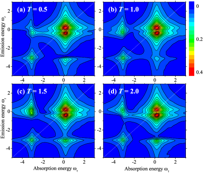
Figure 3: Time evolution of the amplitude of the 2DS spectrum, $\left|\mathcal{A}(\omega_{\tau},T,\omega_{t})\right|$, under the same conditions as in Fig. 2.

As a concrete example, we consider the 2DS spectrum of Fermi polarons at the momentum $\mathbf{K}=0$ in two-dimensions, in line with the relevant experiment on monolayer TMD materials Dey2016 ; Hao2016NatPhys ; Hao2016NanoLett . For the convenience of numerical calculations, we distribute $N$ fermionic atoms on a discrete square lattice ($L\times L$) with a hopping strength $t_{c}$. We assume the impurity has the same hopping strength or mass as the fermionic atoms (i.e., $t_{c}=t_{d})$, so both of them have the same dispersion relation $\epsilon_{\mathbf{k}}=-2t_{c}[\cos(k_{x})+\cos(k_{y})]=\epsilon_{\mathbf{k}}^{I}$. We also take a relatively strong interaction $U=-8t_{c}$, which within Chevy ansatz leads to an attractive polaron energy $E_{A}\simeq-3.08t_{c}$ with residue $Z_{A}\simeq 0.24$ and repulsive polaron energy $E_{R}\simeq+0.15t_{c}$ with residue $Z_{R}\simeq 1-Z_{A}$ at $N=20$ and $L=20$, as illustrated in Fig. 1(a). By varying $N$ and $L$ at a filling factor $N/L^{2}\sim 0.05$, we have checked that the finite size effect is insignificant. Throughout the work, we have used a spectral broadening of $0.2t_{c}$, to better illustrate the 2DS spectrum.

2DS at T=0. Figure 2 presents the amplitude and real part of $\mathcal{A}(\omega_{\tau},T=0,\omega_{t})$ and its symmetric ($\mathcal{A}_{s}$) and asymmetric ($\mathcal{A}_{a}$) components. At zero mixing time $T=0$, $\mathcal{A}_{s}$ can be rewritten as $\mathcal{A}_{s}(\omega_{\tau},T=0,\omega_{t})=G(\omega_{\tau})G^{*}(\omega_{t})/\pi^{2}$, where $G(\omega)=\sum_{n}Z^{(n)}/(\omega+i0^{+}-\mathcal{E}_{n})$ is the retarded impurity Green function Massignan2014 . Therefore, it naturally leads to the two off-diagonal crosspeaks at $(\omega_{\tau},\omega_{t})=(E_{A},E_{R})$ and $(E_{R},E_{A})$ with weight $Z_{A}Z_{R}$, in addition to the two diagonal peaks at $(\omega_{\tau},\omega_{t})=(E_{A},E_{A})$ and $(E_{R},E_{R})$. The two crosspeaks are strongly affected by the asymmetric one-particle-hole contribution $\mathcal{A}_{a}$, which peaks at the upper crosspeak $(E_{R},E_{A})$ in amplitude (see Fig. 2(c)). As a result, the two crosspeak become highly asymmetric, as shown in Fig. 2(a). $\mathcal{A}_{a}$ is also significant near the diagonal peak at the repulsive energy $(E_{R},E_{R})$, forming a side peak slightly below it.

Quantum oscillations. The existence of the two highly asymmetric crosspeaks in 2DS spectrum is a strong evidence of the quantum coherence between attractive and repulsive polarons. Further smoking-gun confirmation can be provided by quantum beats between the crosspeaks at different mixing time $T$, as reported in Fig. 3. From the expression of $\mathcal{A}(\omega_{\tau},T,\omega_{t})$ in Eq. (3), it is readily understood that these beats are caused by the term $e^{-i\left(\mathcal{E}_{n}-\mathcal{E}_{m}\right)T}$, which leads to an oscillation with periodicity $2\pi/\left|E_{A}-E_{R}\right|$ and decay rate $\Gamma_{R}$, where $\Gamma_{R}$ is the decay rate of the repulsive polaron Massignan2014 ; Massignan2011 . This term does not affect the two diagonal peaks, so the 2D spectrum near them is essentially independent on the mixing time $T$, as can be seen from Fig. 3.

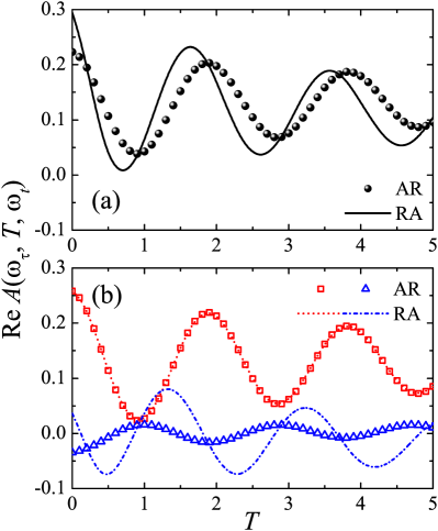
To better characterize the quantum oscillations, we study $\textrm{Re}\mathcal{A}(\omega_{\tau},T,\omega_{t})$ at the two crosspeaks, respectively labelled as AR (lower crosspeak) and RA (higher crosspeak). As shown in Fig. S1 of Supplemental Material SM , despite the same periodicity, interestingly, the two oscillations at AR and RA crosspeaks are not synchronized. The different phases of the two oscillations could be due to the term $e^{-i\delta\mathcal{E}_{\mathbf{k}_{p}\mathbf{k}_{h}}T}$ in the asymmetric one-particle-hole component $\mathcal{A}_{a}$. Indeed, we find $\textrm{Re}\mathcal{A}_{a}$ behaves very different at AR and RA, in sharp contrast to $\textrm{Re}\mathcal{A}_{s}$, which gives the exactly same value at the two crosspeaks.

Relevance to 2DCS. We now compare our theoretical results to the recent 2DCS experiment on Fermi polarons consisting of excitons and trions in monolayer TMD materials Hao2016NanoLett . Although the ways for implementing 2D spectroscopy are different, our simulated 2DS spectrum for Fermi polarons reproduce the key experimental observations Hao2016NanoLett , such as the appearance of the two off-diagonal crosspeaks and their quantum beats as a function of the mixing time $T$. Thereby, in principle our microscopic many-body calculation presents an exciting full ab initio account of the 2DCS spectroscopy of mobile polaron, which has never been achieved, to the best of our knowledge.

Conclusions. We have predicted that quantum beats between the two off-diagonal crosspeaks in the recently proposed two-dimensional Ramsey spectroscopy Wang2022PRX for Fermi polarons are ideally suited to unveil the quantum coherence between the attractive and repulsive polaron branches. Our theoretical results are able to capture the key features of a recent experiment on Fermi polaron-excitons in atomically thin transition metal dichalcogenides Hao2016NanoLett and could be quantitatively verified in highly controllable cold-atom experiments in the near future.

I Supplemental Materials

I.1 Derivation of 1D spectroscopy

In this Supplemental Material, we give a derivation of the conventional 1D Ramsey response and spectral function. In 1D Ramsey scheme, only one $\pi/2$ rf pulse is applied before the last detection pulse at time $\tau$, which gives the final state

$$\left|\psi_{f}\right\rangle=\mathcal{U}\left(\tau\right)\frac{d_{\mathbf{K}\uparrow}^{\dagger}+d_{\mathbf{K}\downarrow}^{\dagger}}{\sqrt{2}}\otimes\left|\textrm{FS}\right\rangle.$$

The Ramsey response can be obtained by measuring $\sigma_{-}=\sigma_{x}-i\sigma_{y}=2\hat{s}_{-}$,

$$\tilde{S}_{a}(\tau)=2\left\langle\psi_{f}\left|\hat{s}_{-}\right|\psi_{f}\right\rangle=\left\langle\textrm{FS}\right|d_{\mathbf{K}\downarrow}\hat{I}_{a}d_{\mathbf{K}\uparrow}^{\dagger}\left|\textrm{FS}\right\rangle,$$ (S1)

where the pathway is given by

$$\hat{I}_{a}\equiv e^{i\mathcal{H}_{\downarrow}\tau}\hat{s}_{-}e^{-i\mathcal{H}_{\uparrow}\tau}.$$ (S2)

Measurement of $\sigma_{-}$ is in consistent with the 2DS measurement of $-\sigma_{+}$ with three $\pi/2$ pulses and $t=T=0$. The additional two instantaneous $\pi/2$ pulses can be recognized as a unitary transformation $U_{\pi}=i\sigma_{y}$, which gives $-U_{\pi}^{\dagger}\sigma_{+}U_{\pi}=\sigma_{-}$.

We expand the time evolution operators as ($t^{\prime}=\tau,T,t$),

$$e^{\pm i\mathcal{H}_{\uparrow}t^{\prime}} = \sum_{n\mathbf{k}}e^{\pm iE_{\uparrow}^{(n)}(\mathbf{k})t^{\prime}}\left|n;\mathbf{k}\right\rangle\left\langle n;\mathbf{k}\right|,$$

$$e^{\pm i\mathcal{H}_{\downarrow}t^{\prime}} = \sum_{\vec{\kappa}_{\nu}\mathbf{k}}e^{\pm iE_{\downarrow}^{(\vec{\kappa}_{\nu})}(\mathbf{k})t^{\prime}}\left|\vec{\kappa}_{\nu};\mathbf{k}\right\rangle\left\langle\vec{\kappa}_{\nu};\mathbf{k}\right|,$$

with polaron states (with index $n$)

$$\left|n;\mathbf{k}\right\rangle =\sum_{\vec{\kappa}_{\nu}}\phi_{\vec{\kappa}_{\nu}}^{(n)}\left(\mathbf{k}\right)d_{\mathbf{k}-\mathbf{k}_{\vec{\kappa}_{\nu}}\uparrow}^{\dagger}\left|\vec{\kappa}_{\nu}\right\rangle,$$

where $\left|\vec{\kappa}_{\nu}\right\rangle=\prod_{i=1}^{\nu}c_{\mathbf{k}_{p}^{(i)}}^{\dagger}\prod_{i=1}^{\nu}c_{\mathbf{k}_{h}^{(i)}}\left|\textrm{FS}\right\rangle$ denotes $\nu$ particle-hole pairs excitations on top of a Fermi sea, $\vec{\kappa}_{\nu}\equiv\{\mathbf{k}_{p}^{(1)},\mathbf{k}_{p}^{(2)},\cdots,\mathbf{k}_{p}^{(\nu)};\mathbf{k}_{h}^{(1)},\mathbf{k}_{h}^{(2)},\cdots,\mathbf{k}_{h}^{(\nu)}\}$ is a collective notation for the $\nu$ particle momenta ($\mathbf{k}_{p}^{(i)}>k_{F}$) and hole momenta ($\mathbf{k}_{h}^{(i)}<k_{F}$), and therefore the total momentum and energy of the particle-hole excitations are given by $\mathbf{k}_{\vec{\kappa}_{\nu}}\equiv\sum_{i=1}^{\nu}[\mathbf{k}_{p}^{(i)}-\mathbf{k}_{h}^{(i)}]$ and $\epsilon_{\vec{\kappa}_{\nu}}=\sum_{i=1}^{\nu}[\epsilon_{\mathbf{k}_{p}^{(i)}}-\epsilon_{\mathbf{k}_{h}^{(i)}}]$, respectively. The energy of the ($n$-th) polaron state can be denoted as, $\mathcal{E}_{n}(\mathbf{k})=E_{\uparrow}^{(n)}(\mathbf{k})-(\epsilon_{\mathbf{k}}^{I}+\omega_{s}+E_{\textrm{FS}})$, after the subtraction of the impurity energy ($\epsilon_{\mathbf{k}}^{I}+\omega_{s}$) and the energy of the background Fermi sea ($E_{\text{FS}}$). On the other hand, the many-body eigenstates in the case of the spin-down impurity are much simpler and can be directly characterized by $\vec{\kappa}_{\nu}$, i.e., $\left|\vec{\kappa}_{\nu};\mathbf{k}\right\rangle=d_{\mathbf{k}-\mathbf{k}_{\vec{\kappa}_{\nu}}\downarrow}^{\dagger}\left|\vec{\kappa}_{\nu}\right\rangle$. The corresponding energy is given by, $\delta\mathcal{E}_{\vec{\kappa}_{\nu}}(\mathbf{k})=E_{\downarrow}^{(\vec{\kappa}_{\nu})}(\mathbf{k})-(\epsilon_{\mathbf{k}}^{I}+E_{\textrm{FS}})=\epsilon_{\vec{\kappa}_{\nu}}+\epsilon_{\mathbf{\mathbf{k}-\mathbf{k}_{\vec{\kappa}_{\nu}}}}^{I}-\epsilon_{\mathbf{k}}^{I}$, which is a summation of the recoil energy of the impurity and the Fermi sea.

Inserting the expansion of time evolution operators into $\tilde{S}_{A}(\tau)$ gives the 1D Ramsey response

$$\tilde{S}_{A}(\tau)=\sum_{n}e^{-i\mathcal{E}_{n}(\mathbf{k})t}\phi_{0}^{(n)*}\phi_{0}^{(n)}\equiv\sum_{n}e^{-i\mathcal{E}_{n}(\mathbf{k})t}Z^{(n)},$$ (S3)

which is related with the spectral function $\mathcal{A}_{A}(\omega_{\tau})$ by a Fourie transformation

$$\mathcal{A}_{A}(\omega_{\tau})=\frac{1}{\pi}\int_{0}^{\infty}d\tau e^{i(\omega_{\tau}+\omega_{s})\tau}\tilde{S}_{A}(\tau)=\frac{1}{\pi}\sum_{n}\frac{Z^{(n)}}{\omega_{\tau}^{+}-\mathcal{E}_{n}},$$ (S4)

where we omit the dependence of $\mathbf{K}$ in $Z^{(n)}(\mathbf{K})$ and $\mathcal{E}_{n}(\mathbf{K})$ for simplicity of notation. These expressions is in consistent with previous studies (Massignan2014, ; Schmidt2018, ).

I.2 Quantum oscillations at the crosspeaks

Fig. S1: (a) Time-dependent real part of the 2DS $\textrm{Re}\mathcal{A}(\omega_{\tau},T,\omega_{t})$ at the lower crosspeak (AR, black circles) and the higher crosspeaks (RA, black solid line). (b) $\textrm{Re}\mathcal{A}_{s}(\omega_{\tau},T,\omega_{t})$ (red dashed line and squares) and $\textrm{Re}\mathcal{A}_{a}(\omega_{\tau},T,\omega_{t})$ (blue dot-dashed line and triangles) at the lower crosspeak (AR, symbols) and the higher crosspeaks (RA, lines). Other parameters are the same as in Fig. 2 in the main text.

To illustrate the quantum oscillations at the crosspeaks in details, we show $\textrm{Re}\mathcal{A}(\omega_{\tau},T,\omega_{t})$ at the two crosspeaks, respectively labelled as AR (lower crosspeak) and RA (higher crosspeak) as a function of $T$ in Fig. (S1). As shown in Fig. S1(b) $\textrm{Re}\mathcal{A}_{a}$ behave very different at AR and RA (see the blue triangles and dot-dashed line). This is in sharp contrast to $\textrm{Re}\mathcal{A}_{s}$, which gives the exactly same value at the two crosspeaks (see the overlapping red squares and dotted line).

References

(1)A. S. Alexandrov and J. T. Devreese, Advances
in Polaron Physics (Springer, New York, 2010), Vol. 159.
(2)L. D. Landau, Electron Motion in Crystal Lattices,
Phys. Z. Sowjetunion 3, 664 (1933).
(3)A. C. Hewson, The Kondo Problem to Heavy
Fermions (Cambridge University Press, Cambridge, 1993).
(4)P. W. Anderson, Infrared Catastrophe in Fermi
Gases with Local Scattering Potentials, Phys. Rev. Lett. 18,
1049 (1967).
(5)G. D. Mahan, Excitons in Metals: Infinite Hole
Mass, Phys. Rev. 163, 612 (1967).
(6)B. Roulet, J. Gavoret, and P. Nozières, Singularities
in the X-Ray Absorption and Emission of Metals. I. First-Order Parquet
Calculation, Phys. Rev. 178, 1072 (1969).
(7)P. Nozières and C. T. De Dominicis, Singularities
in the X-Ray Absorption and Emission of Metals. III. One- Body Theory
Exact Solution, Phys. Rev. 178, 1097 (1969).
(8)Y. Nagaoka, Ferromagnetism in a Narrow, Almost
Half-Filled Band, Phys. Rev. 147, 392 (1966).
(9)B. S. Shastry, H. R. Krishnamurthy, and P. W.
Anderson, Instability of the Nagaoka ferromagnetic state of the
Hubbard model, Phys. Rev. B 41, 2375 (1990).
(10)A. G. Basile and V. Elser, Stability of the ferromagnetic
state with respect to a single spin flip: Variational calculations
for the Hubbard model on the square lattice, Phys. Rev.
B 41, 4842(R) (1990).
(11)D. N. Sheng, Y. C. Chen, and Z. Y. Weng, Phase
String Effect in a Doped Antiferromagnet, Phys. Rev. Lett. 77,
5102 (1996).
(12)I. Bloch, J. Dalibard, and W. Zwerger, Many-body
physics with ultracold gases, Rev. Mod. Phys. 80, 885 (2008).
(13)C. Chin, R. Grimm, P. Julienne, and E. Tiesinga,
Feshbach resonances in ultracold gases, Rev. Mod. Phys. 82,
1225 (2010).
(14)A. Schirotzek, C.-H. Wu, A. Sommer, and M.W.
Zwierlein, Observation of Fermi Polarons in a Tunable Fermi Liquid
of Ultracold Atoms, Phys. Rev. Lett. 102, 230402 (2009).
(15)Y. Zhang, W. Ong, I. Arakelyan, and J. E. Thomas,
Polaron-to-Polaron Transitions in the Radio-Frequency Spectrum of
a Quasi-Two-Dimensional Fermi Gas, Phys. Rev. Lett. 108,
235302 (2012).
(16)C. Kohstall, M. Zaccanti, M. Jag, A. Trenkwalder,
P. Massignan, G.M. Bruun, F. Schreck, and R. Grimm, Metastability
and coherence of repulsive polarons in a strongly interacting Fermi
mixture, Nature (London) 485, 615 (2012).
(17)M. Koschorreck, D. Pertot, E. Vogt, B. Fröhlich,
M. Feld, and M. Köhl, Attractive and repulsive Fermi polarons in two
dimensions, Nature (London) 485, 619 (2012).
(18)M. Cetina, M. Jag, R. S. Lous, I. Fritsche, J.
T. M.Walraven, R. Grimm, J. Levinsen, M. M. Parish, R. Schmidt, M.
Knap, and E. Demler, Ultrafast many-body interferometry of impurities
coupled to a Fermi sea, Science 354, 96 (2016).
(19)F. Scazza, G. Valtolina, P. Massignan, A. Recati,
A. Amico, A. Burchianti, C. Fort, M. Inguscio, M. Zaccanti, and G.
Roati, Repulsive Fermi Polarons in a Resonant Mixture of Ultracold
6Li Atoms, Phys. Rev. Lett. 118, 083602 (2017).
(20)M.-G. Hu, M. J. Van de Graaff, D. Kedar, J. P. Corson,
E. A. Cornell, and D. S. Jin, Bose Polarons in the Strongly Interacting
Regime, Phys. Rev. Lett. 117, 055301 (2016).
(21)N. B. Jørgensen, L. Wacker, K. T. Skalmstang,
M. M. Parish, J. Levinsen, R. S. Christensen, G. M. Bruun, and J.
J. Arlt, Observation of Attractive and Repulsive Polarons in a Bose-Einstein
Condensate, Phys. Rev. Lett. 117, 055302 (2016).
(22)P. Massignan, M. Zaccanti, and G. M. Bruun,
Polarons, dressed molecules and itinerant ferromagnetism in ultracold
Fermi gases, Rep. Prog. Phys. 77, 034401 (2014).
(23)Z. Lan and C. Lobo, A single impurity in an ideal
atomic Fermi gas: current understanding and some open problems, J.
Indian Inst. Sci. 94, 179 (2014).
(24)R. Schmidt, M. Knap, D. A. Ivanov, J.-S. You,
M. Cetina, and E. Demler, Universal many-body response of heavy impurities
coupled to a Fermi sea: a review of recent progress, Rep. Prog. Phys.
81, 024401 (2018).
(25)X. Cui and H. Zhai, Stability of a fully magnetized
ferromagnetic state in repulsively interacting ultracold Fermi gases,
Phys. Rev. A 81, 041602(R) (2010).
(26)P. Massignan and G. M. Bruun, Repulsive polarons
and itinerant ferromagnetism in strongly polarized Fermi gases, Eur.
Phys. J. D 65, 83 (2011).
(27)O. Goulko, A. S. Mishchenko, N. Prokof’ev, and
B. Svistunov, Dark continuum in the spectral function of the resonant
Fermi polaron, Phys. Rev. A 94, 051605(R) (2016).
(28)J. Wang, X.-J. Liu, and H. Hu, Exact Quasiparticle
Properties of a Heavy Polaron in BCS Fermi Superfluids, Phys. Rev.
Lett. 128, 175301 (2022).
(29)J. Wang, X.-J. Liu, and H. Hu, Heavy polarons
in ultracold atomic Fermi superfluids at the BEC-BCS crossover: Formalism
and applications, Phys. Rev. A 105, 043320 (2022).
(30)M. Knap, A. Shashi, Y. Nishida, A. Imambekov, D.
A. Abanin, and E. Demler, Time-Dependent Impurity in Ultracold Fermions:
Orthogonality Catastrophe and Beyond, Phys. Rev. X 2, 041020
(2012).
(31)J. Wang, Multidimensional Spectroscopy of Time-Dependent
Impurities in Ultracold Fermions, arXiv:2207.10501 (2022).
(33)X. Li, T. Zhang, C. N. Borca, and S. T. Cundiff,
Many-Body Interactions in Semiconductors Probed by Optical Two-Dimensional
Fourier Transform Spectroscopy, Phys. Rev. Lett. 96, 057406
(2006).
(35)J. A. Davis, L. V. Dao, M. T. Do, P. Hannaford,
K. A. Nugent, and H. M. Quiney, Noninterferometric Two-Dimensional
Fourier-Transform Spectroscopy of Multilevel Systems, Phys. Rev. Lett.
100, 227401 (2008).
(36)G. Nardin, T. M. Autry, G. Moody, R. Singh, H.
Li, and S. T. Cundi, Multidimensional coherent optical spectroscopy
of semiconductor nanostructures: Collinear and non-collinear approaches,
J. Appl. Phys. 177, 112804 (2015).
(37)P. Dey, J. Paul, Z. Wang, C. E. Stevens, C. Liu,
A. H. Romero, J. Shan, D. J. Hilton, and D. Karaiskaj, Optical Coherence
in Atomic-Monolayer Transition-Metal Dichalcogenides Limited by Electron-Phonon
Interactions, Phys. Rev. Lett. 116, 127402 (2016).
(38)K. Hao, G. Moody, F. Wu, C. K. Dass, L. Xu,
C.-H. Chen, L. Sun, M.-Y. Li, L.-J. Li, A. H. MacDonald, and X. Li,
Direct measurement of exciton valley coherence in monolayer WSe2,
Nat. Phys. 12, 677 (2016).
(39)K. Hao, L. Xu, P. Nagler, A. Singh, K. Tran,
C. K. Dass, C. Schuller, T. Korn, X. Li, and G. Moody, Coherent and
incoherent coupling dynamics between neutral and charged excitons
in monolayer MoSe2, Nano Lett. 16, 5109 (2016).
(40)R. Tempelaar and T. C. Berkelbach, Many-body
simulation of two-dimensional electronic spectroscopy of excitons
and trions in monolayer transition metal dichalcogenides, Nat. Commun.
10, 3419 (2019).
(41)J. B. Muir, J. Levinsen, S. K. Earl, M. A. Conway,
J. H. Cole, M. Wurdack, R. Mishra, D. J. Ing, E. Estrecho, Y. Lu,
D. K. Efimkin, J. O. Tollerud, E. A. Ostrovskaya, M. M. Parish, and
J. A. Davis, Exciton-polaron interactions in monolayer WS2,
arXiv:2206.12007 (2022).
(42)Lachlan P Lindoy, Yao-Wen Chang and David R
Reichman, Two-Dimensional Spectroscopy of Two-Dimensional Materials,
arXiv:2206.01799 (2022).
(43)M. Sidler, P. Back, O. Cotlet, A. Srivastava,
T. Fink, M. Kroner, E. Demler, and A. Imamoglu, Fermi polaron-polaritons
in chargetunable atomically thin semiconductors, Nat. Phys. 13,
255 (2017).
(44)D. K. Efimkin and A. H. MacDonald, Many-body
theory of trion absorption features in two-dimensional semiconductors,
Phys. Rev. B 95, 035417 (2017).
(45) In the Supplemental Materials, we show (1) a derivation of the 1DS
that agrees with previous studies and (2) some details of the quantum oscillations
at two crosspeaks.
(46)F. Chevy, Universal phase diagram of a strongly
interacting Fermi gas with unbalanced spin populations, Phys. Rev.
A 74, 063628 (2006).
(47)M. M. Parish and J. Levinsen, Quantum dynamics
of impurities coupled to a Fermi sea, Phys. Rev. B 94, 184303