Quantum Vulnerability Analysis to Accurate Estimate the Quantum Algorithm Success Rate

Abstract

Quantum technology is still in its infancy, but superconducting circuits have made great progress toward pushing forward the computing power of the quantum state of the art. Due to limited error characterization methods and temporally varying error behavior, quantum operations can only be quantified to a rough percentage of successful execution, which fails to provide an accurate description of real quantum execution in the current noisy intermediate-scale quantum (NISQ) era. State-of-the-art success rate estimation methods either suffer from significant prediction errors or unacceptable computation complexity. Therefore, there is an urgent need for a fast and accurate quantum program estimation method that provides stable estimation with the growth of the program size. Inspired by the classical architectural vulnerability factor (AVF) study, we propose and design Quantum Vulnerability Factor (QVF) to locate any manifested error which generates Cumulative Quantum Vulnerability (CQV) to perform SR prediction. By evaluating it with well-known benchmarks on three 27-qubit and one 65-qubit quantum machines, CQV outperforms the state-of-the-art prediction technique ESP by achieving on average 6 times less relative prediction error, with best cases at 20 times, for benchmarks with a real SR rate above 0.1%.

1 Introduction

Superconducting quantum computing [1, 3, 31] is one of the major technologies of quantum computing that aims to solve problems that are intractable on a classical computer by leveraging mature silicon technology. Compared to other quantum computing hardware technologies, it has advantages in scalability, microwave operation control, and nanosecond-level gate operation [9, 8, 5].

Figure 1: One complete cycle of validating new quantum ideas with proposed CQV as SR estimator, bypassing the real quantum machine. Original image from [29]

However, superconducting quantum computers suffer from a great variety of noise channels, which can be classified into retention errors or operational errors [34].

Although quantum error correction (QEC) can be performed to fix the errors, this requires an enormous number of physical qubits that cannot be realized in current noisy intermediate-scale quantum (NISQ) era machines which contain at most a few hundred noisy qubits [25]. Therefore, in NISQ, quantum computing performs noisy operations and accepts the fact that errors can happen on any physical qubit at any time during the execution. To combat the high error rate, correct output is captured by repeating the same computations for a sufficient number of trials, and the number of correct trials out of the total number of trials is called Success Rate (SR).

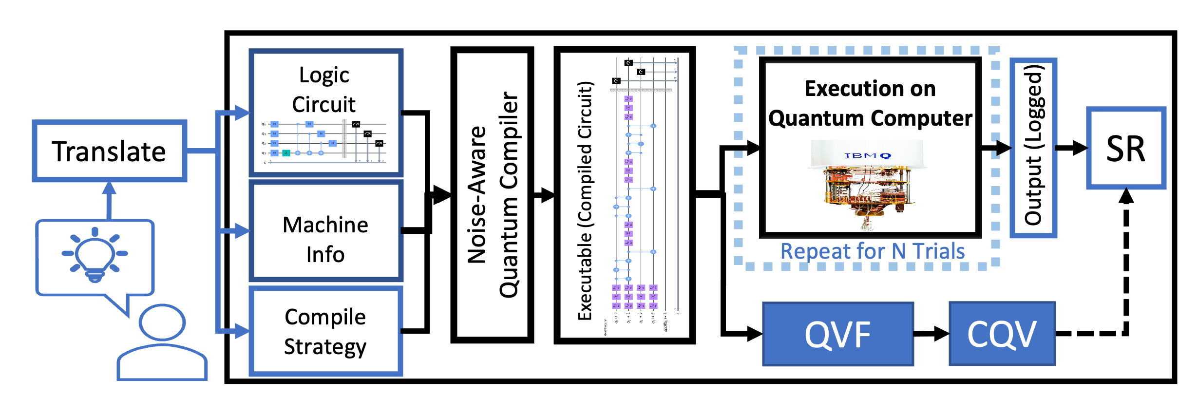
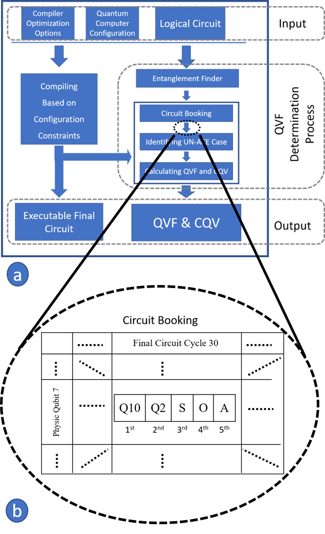
Figure 1 shows one complete validation round of a researcher testing a new idea, and the idea needs to be transferred to a compiled circuit before executing on a real machine. Repeatedly waiting for results executed by noisy, crowded, and privileged quantum computers to validate designs is becoming an unavoidable bottleneck for researchers in many quantum computing fields, revealing the demand for an alternative way to easily and quickly get the final SR.

Surprisingly, compared with the popular research on improving the success rate, fewer studies are trying to understand how a given compiled circuit results in a certain experimental success rate after executing on a target quantum computer. The reason behind that is the lack of an accurate method to model the error and simulate the cumulative success rate based on that. Knowing the error behavior is one of the unavoidable prerequisites for improving the success rate and knowing how much and where to reduce the errors.

Currently, there are two ways to predict the success rate: the estimated probability of success (ESP) [32] and statistical fault injection [14]. Both suffer from low accuracy and increasing prediction errors when algorithm size is increased. Inspired by the famous classical chip vulnerability study AVF [35, 6], we have proposed and designed a quantum vulnerability factor (QVF) that locates error matter qubits and applies an accurate error modeling scheme to generate a cumulative quantum vulnerability (CQV). As shown in Fig. 1, the CQV would simulate the error behaviors for the target quantum chip and estimate the SR.

To predict the SR, we first redesign the compiled circuits to enable cycle view, promising each physical qubit will be involved with at most one operation within a cycle, which isolates errors to cycles. Next, based on the observation that some errors do not impact the output, we define such qubits to be in an un-architecturally correct execution required (un-ACE) state for the given cycle and exhausted all possible cases of un-ACE state. Then, based on the ACE states, we calculated the QVF and applied it to help the calculation of CQV. In addition, by presenting the un-ACE states for every gate at the compiled time, researchers will have a clear and direct view of gate error behaviors straight from the compiled circuit. Ultimately, the CQV is calculated by accumulating the gate success rate, which is calculated from calibrated gate errors including the crosstalk error, through all the ACE states within the QVF model. The error modeling scheme of CQV also presents a novel and accurate way to quantify the error impact across the CNOT gates and produce the 1-CQV in the end for predicting actual SR for a given system.

We validate our design on four of the state-of-the-art quantum machines with 27 and 65 qubits hosted by IBM written with the Qiskit open-source quantum platform [14]. As a quantum system SR estimator, with the pre-calibrated system on a different day, the CQV outperforms the state-of-the-art SR estimator ESP by reducing on average 6 times in relative prediction error, with best cases at 20 times. We also verify that the CQV can achieve good accuracy for unseen benchmarks and unseen machines.

The contributions of our paper can be listed as follows:

• To our best knowledge, we are the first to bring the classical vulnerability study analysis to the quantum computing analyses, which changes the way of viewing errors and compiled circuits.

• We define and propose a systematic methodology to demonstrate all possible different un-ACE state cases.

• We design and build an accurate and simple error modeling scheme in which the first work quantifies error impact flowing across the CNOT gate.

• The proposed CQV outperforms the current state-of-the-art success rate estimation model and achieves 6 times less relative prediction error on average.

• When the size of the algorithm reaches and surpasses the quantum volume of a device, the CQV has a 10x improvement in relative prediction error rate compared with the state-of-the-art estimates.

2 Background

2.1 Quantum Circuit

The qubit is the quantum counterpart of the classical bit, capable of taking state $|0\rangle$, state $|1\rangle$, and all the other linear combinations of the $|0\rangle$ and $|1\rangle$ states. A $CNOT$ gate is the two-qubit gate that reverses the magnitude of the target qubit if the input state of the control qubit’s magnitude is at state one. During the CNOT operation, the phase information on the target qubit’s state will transfer through the $CNOT$ gate and apply to the control qubit’s state at the output, which is known as phase-kickback. The SWAP gate is used when performing state exchange of two qubits, which is equivalent to three $CNOT$ gates in series.

The processes of generating a quantum executable from a given algorithm and executing it on a quantum chip have been shown in Figure 1. The logical circuits are generated assuming an all-to-all connection between qubits, which can be applied on a superconducting quantum computer, which supports only adjacent connections, after a series of compiling steps. As shown, the quantum compiler will be given information about the target quantum chip and compiler strategy, such as optimization levels, initial layout method, mapping method, etc. Based on that, the compiler will follow all the intermediate compiling steps to generate a compiled circuit for executing on the quantum computer. For more details on quantum computing, please refer to [23].

2.2 NISQ Era Quantum Error

Superconducting quantum computers are currently one of the most promising technologies for quantum computation, with advantages in scalability, operation control, operating on nanosecond scale, microwave control, etc. However, noise is the biggest challenge that impedes the growth of superconducting quantum computing toward solving large-size algorithms. The noise that a superconducting quantum computer suffers can be classified as operational errors and retention errors [34].

Operational Errors: When operating a superconducting quantum computer, the control pulses for gate operations may introduce errors into the target qubits’ quantum state or the nearby qubits. For instance, on 4/21/2022 the ibmq_montreal quantum chip had an average single-qubit operation error rate at $5.04\times 10^{-4}$, average measurement error rate at $3.05\times 10^{-2}$, and average CNOT error rate at $2.11\times 10^{-2}$ [13], which varies over time. More complex forms of operational errors exist, such as the recently observed crosstalk errors [22].

Retention Errors: The lifetime of a qubit is determined by its relaxation time (T1) and decoherence time (T2). The decoherence and relaxation time represent the qubit’s average time to retain its energized and superpositioned states, respectively. These times act as an upper limit for the current quantum computing execution time.

Figure 2: Current success rate estimator performance

Success Rate: While performing computation on current quantum computers, errors can occur at almost every qubit and every cycle with a frequency as high as once in every few hundred cycles. The solution to such noisy computation is Quantum Error Correction (QEC), correcting the noise and achieving fault-tolerant quantum computing. However, QEC cannot be applied in the current Noise-Intermediate Scale Quantum Computers (NISQ) machines, defined as machines with noisy qubits ranging from a few tens to a few hundred [25]. Quantum computers in the NISQ class do not have enough qubits to perform QEC. Therefore, the current quantum computers use repetition methods to increase the chance of getting correct output results against the noise as shown in Figure 1. The current number of repetitions can range from a few hundred to a few thousand. We compute the Success Rate (SR) by dividing the number of correct outputs by the total number of executions, which is shown in equation 1. The Failure Rate (FR) is the counterpart driven by one minus the SR.

$$Success\ Rate=\frac{Number\ of\ trials\ with\ correct\ output}{Number\ of\ N\ repeated\ trails\ }\$$ (1)

Figure 3: ESP for different circuits

3 Motivation

3.1 Limitations of Success Rate Metric

Currently, quantum algorithms are evaluated mainly based on the success rate metric, or metrics derived from success rate, such as PST or MIBF[34]. However, the success rate has a few inherent drawbacks at both hardware and software levels, which prevents it to be used directly to study the error behavior.

The first problem is that the correct result must be known in advance, either through mathematical predictions or simulated executions on a classical computer[14]. Superconducting quantum computers are currently one of the most promising technologies for quantum computation, with advantages in scalability, operation control, operating on nanosecond scale, microwave control, etc. However, noise is the biggest challenge that impedes the growth of superconducting quantum computing toward solving large-size algorithms.

3.2 Limitations of Current Error Analyzing Methods

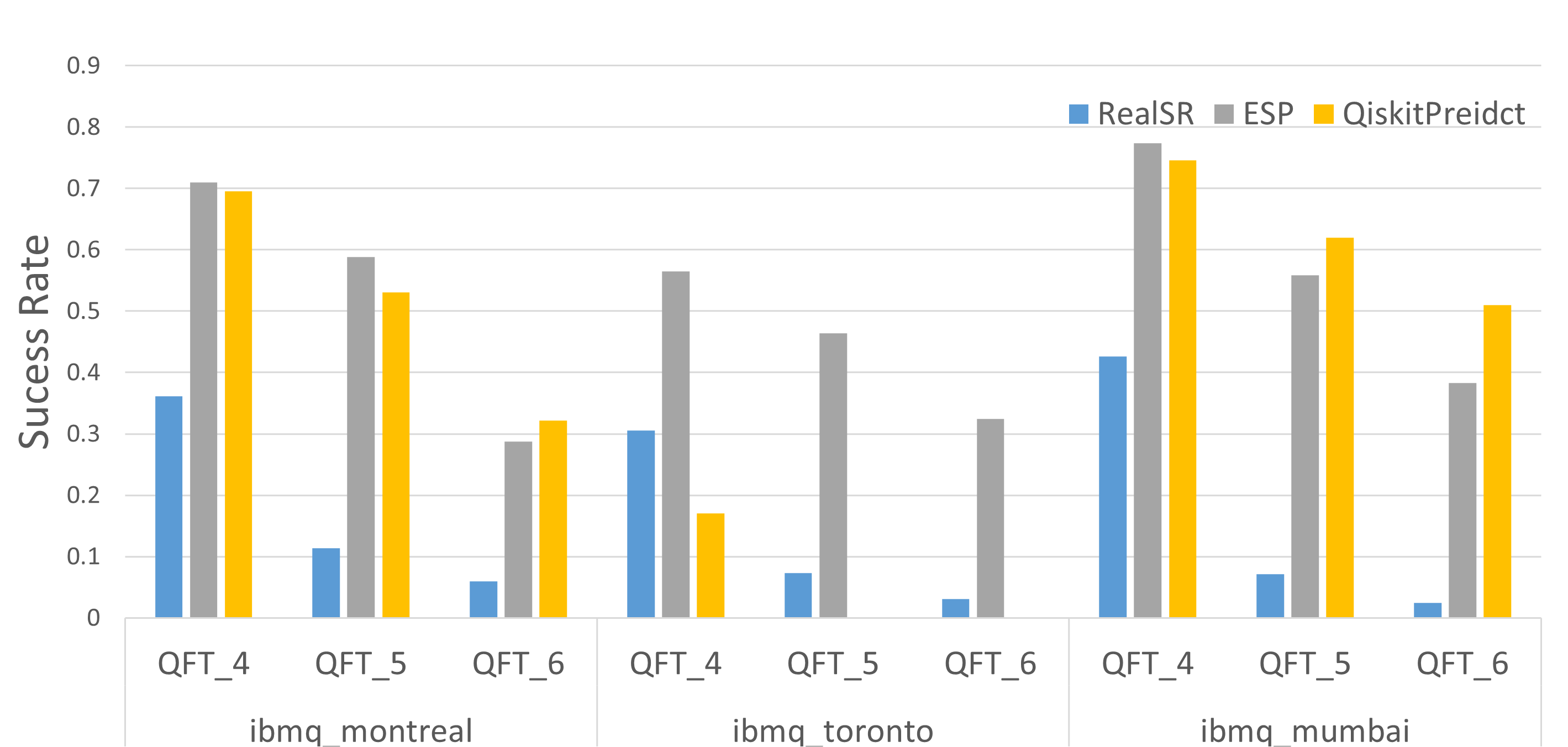
Currently, compared with error modeling studies, research on improving the success rate by optimizing the compiler strategy has been receiving more focus, which is presented in detail in section 11. Among the existing methods of predicting SR, the major two are statistical fault injection [13] and estimated success probability (ESP) [32]. Statistical Fault Injection utilizes the classical computer to simulate the quantum computation with errors injected to each basis gate with certain triggering probabilities and log the output[14]. Such a method has an inherent problem of scale-up. The estimated success probability (ESP), shown in equation 3, predicts the correct output trial probability by multiplying the success rate of each gate, generated by one minus the error rate in equation 2, for the full circuit. As shown in Fig. 2, we have applied both methods to estimate the SR of the QFT algorithm with various algorithm sizes and quantum chips. The predicted results of both methods fail to capture the real SR with a range of 25% to 60% offset and their relative error rates range from 70% to 470%. Meanwhile, both models have decreased prediction accuracy when the algorithm size gets large, which fails to support scaled-up computing.

$$g_{i}^{s}=(1-g_{i}^{e}),\ m_{i}^{s}=(1-m_{i}^{e})$$ (2)

$$ESP=\displaystyle\prod_{i=1}^{N_{gates}}g_{i}^{s}*\displaystyle\prod_{i=1}^{N_{Measurement}}m_{i}^{s}$$ (3)

3.3 Some Error Matter and Some Do Not

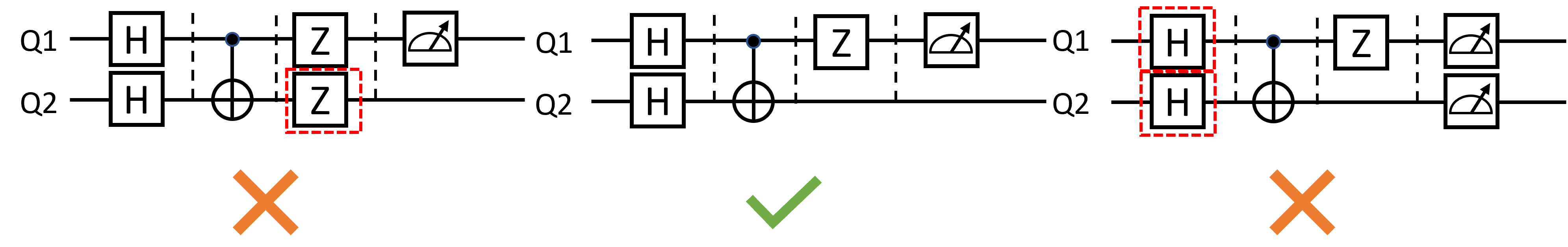
By inspecting compiled circuits based on cycles, we can examine the ESP model to identify why it fails to predict the success rate accurately. As shown in Fig. 3, the ESP model could make a correct prediction of the SR only for the second circuit. It will overestimate the error for cases similar to the first circuit since the error of the red-boxed $Z$ gate cannot impact the final result.

It will also underestimate the error for cases like the third circuit since the error that happened on the two red-boxed $H$ gates will influence both cumulative SRs of the two measurements. However, based on the gate error rate to gate success rate transformation presented in equation 2 from ESP, the impact of such error had been calculated only once. The error effect could be addressed as error propagation and is completely ignored in this model. From such analysis, it is clear that some errors in the compiled circuit are not going to impact the output result no matter what the error states are, and some are making more impact.

Figure 4: Cycle view maps operation and virtual qubit onto quantum chip, with Cumulative SR of the qubit and gate success rate appear for each physical qubit at every cycles

4 Quantum Vulnerability Factor

4.1 Cycle View

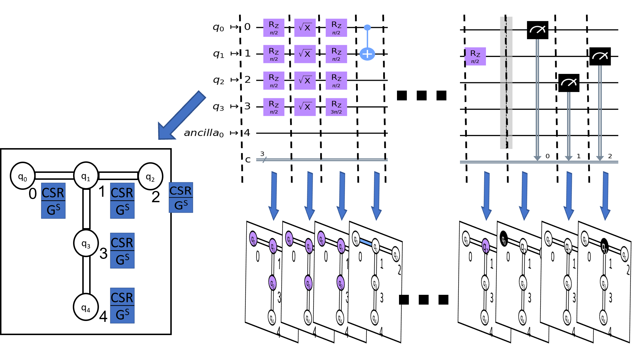
For understanding the error behavior while executing on a quantum chip, a clear view of where and when the error occurs and how much it affects the compiled circuit has to be established first. Therefore, this paper quantifies the compiled circuit to a finer degree, the cycle level, analogous to the classical electrical circuit diagram, as defined in Figure 4, to replace the previous analysis at the level of the entire compiled circuit. Based on the compiled circuit with cycle restrictions, a snapshot of the operating quantum chip at a given cycle can be linked with the corresponding cycle in the compiled circuit. By using the cycle view, at most one type of error will happen to the physical qubit during the cycle time since at most one gate will happen to any physical qubit within a cycle. If we insert identity gates into cycles where physical qubits are idle with corresponding identity operation error rates, the error and gate count of the cycle-view-enabled compiled circuit could be simplified as the production of cycle count and physical qubit count. In addition, each physical qubit at any cycle could display two numbers associated with it identifying its cumulative success rate and current gate success rate. Such error isolation provides a direct view of computation by viewing complicated compiled circuits as clear quantum chip snapshots and assigning time attributes to all the errors.

4.2 Quantum ACE State and QVF

Inspired by the classical architecturally correct execution (ACE) and architectural vulnerability factor (AVF) [35, 6] and error matter example seen in the last section, we develop the Quantum Vulnerability factor (QVF) and Cumulative Quantum Vulnerability (CQV), to locate the overestimate errors and perform error modeling include the error flowing across a CNOT gate, respectfully. The CQV is present in Sec. 6.

The QVF uses the ACE state to represent the cases where the error does not matter. The definition of the un-ACE state: If an error happens to a physical qubit at any given cycle, the infected quantum states will not affect the output bits. In contrast, if an error on a physical qubit at a given cycle might impact the output, the qubit is considered to be in the ACE state. To be conservative, we only change qubits from the ACE to un-ACE state when any incident error that can occur on it at a given cycle cannot change the output. To determine the ACE state, instead of giving a wrong state to a target qubit and simulating the output state like the fault injection method used in Qiskit and other work [26], we focus on determining whether there exists a path between the error and any measurement gate. We have given a detailed description of determining all the cases of the un-ACE state in Sec. 5

After using the cycle view to present errors and identify all un-ACE states out of the circuit, all the left are ACE states. The factor of ACE states over the sum of ACE and un-ACE states for a given time can be used to quantify the vulnerability of the quantum chip, which we name Quantum Vulnerability Factor (QVF). The definition of QVF: For a given compiled circuit arranged in cycle view, the QVF is equal to the average failure rate, which uses the calibrated error rate of the target physical qubit and its operation, of all ACE states over total physical qubits for all the cycles. It can be rewritten as the failure rate of all ACE states across the quantum chip at any given cycle. Identifying more un-ACE states will result in achieving a lower QVF and a better approximation of the real error effect during execution. More un-ACE states mean fewer ACE states and therefore a less vulnerable circuit. Additionally, understanding the ACE states distribution across the chip can guide architects to make trade-offs between cost and reliability when designing future quantum computers. One of the core advantages of QVF is that it can be known at compile time. We summarize acronyms used throughout this work in Table 1.

Table 1: Table of acronyms

Term	Explanation
NOISE	Error rate for Operations or States
ACE	Architecturally Correction Execution
Un-ACE	Unnecessary for Architecturally
	Correction Execution
QVF	Quantum Vulnerability Factor
CQV	Cumulative Quantum Vulnerability
ESP	Estimated Probability of Success
SR	Success Rate of correct result
FR	Failure rate: one minus Success Rate

5 Determining Un-ACE States

5.1 Virtual Qubit Terminology

When identifying un-ACE states, we find that the two different categories, logical and ancilla qubits form the set of virtual qubits which equals the number of physical qubits. Logical qubits are initially defined by a logical circuit and can be divided into outputting logical qubits and assisting logical qubits based on whether the qubit is measured in the end. The virtual qubits added to fill the gap between logical and physical qubits are named ancilla qubits, based on the wildly used concept in the quantum compiling community [13]. Ancilla qubits are further classified as used ancilla qubits and unused ancilla qubits based on whether they participate in computation. In this way, discussing all the un-ACE cases belonging to each type of virtual qubit will cover all the un-ACE cases.

5.2 Ancilla Qubits in the Un-ACE States

The compiler performs expands the number of virtual qubits by adding ancilla qubits as placeholders. For such reason, the ancilla qubits can stay idle for the entire circuit or be used to perform swaps to transfer logical qubits when there are connection limitations among targeted physical qubit pairs. However, when necessary, the compiler can use ancilla qubits to perform operations and later pass the prepared quantum states to the logical qubits. Therefore, ancilla qubits tend to have a smaller chance to meet a two-qubit gate, except for three CNOT gates grouped into a swap gate. Therefore, errors that happen to them have a lower chance to propagate toward output bits. Below are the two cases of ancilla qubit usage and the corresponding ACE analysis.

Case 1: Unused Ancilla Qubits. To determine whether an ancilla qubit can be classified in this case, we must examine its entire lifetime. First, the ancilla qubit should stay in the same physical qubit for the entire circuit, which means that it is not involved in any swap operations. Next, the ancilla qubit must not encounter any operations except for barriers and idle (identity) operations as these do not affect the qubit state. The ancilla qubit in question stays in the un-ACE state in all cycles if meeting these requirements. It is simple to verify as no paths are available to such virtual qubits to spread any error to other virtual qubits.

Figure 5: Un-ACE state cases. 1 and 2): Non-entangled un-ACE states cases. 3-5): Entangled qubits determination cases

Case 2: Used Ancilla Qubits. Ancilla qubits involved in operations other than identity or barrier operations are classified as used ancilla qubits. We choose to consider the used ancilla qubits the same as assisting logical qubits for un-ACE qubit state determination. Since they are both used to prepare quantum states for outputting logical qubits, their primary job is to assist final output. Therefore, errors on the used ancilla qubits can impact the output, and detailed ACE determination steps are presented in section 5.3.

5.3 Logical Qubits in the Un-ACE States

Here we introduce cases and methods to identify un-ACE states for the two categories of logical qubits. The first group are logical qubits that are measured and directly written to at least one of the output bits, which we name as outputting logical qubits. On the contrary, the second group contains the logical qubit that does not have a measurement gate, which is named as assisting logical qubits. Most logical qubits belong to the first group. They tend to stay in the ACE state for most of their cycles, except for the cycles before being initialized and after measurement, where the states are not being used or transferred. The second group is used to prepare the desired quantum state and transfer it to other logical qubits to assist the final output. Therefore, for the qubits in the second group, they become un-ACE after the last time they transfer states. The previously discussed used ancilla qubits overlap with this second group.

However, there are cases where assisting logical qubits can stay in the ACE state even after passing the state. Such cases happen when the virtual qubits are entangled. The entangled correlation between virtual qubits will maintain until either one of the entangled qubits is measured or the entanglement is terminated. Therefore, we will first introduce the process of determining the un-ACE state in non-entangled cases. Then we will present a similar procedure for qubits in entangled cases.

5.3.1 Non-Entangled Logical Qubit in Un-ACE State

In this subsection, the targeted logical qubit will stay non-entangled with any other qubits for the entire circuit time. Here we will introduce how to identify the un-ACE state for both outputting and assisting logical qubits. We choose to inspect the logical qubits’ cycles from end to start (right to left), starting from the last cycle of the circuit. This way, a segment of un-ACE qubit states can be determined in one search until the condition changes.

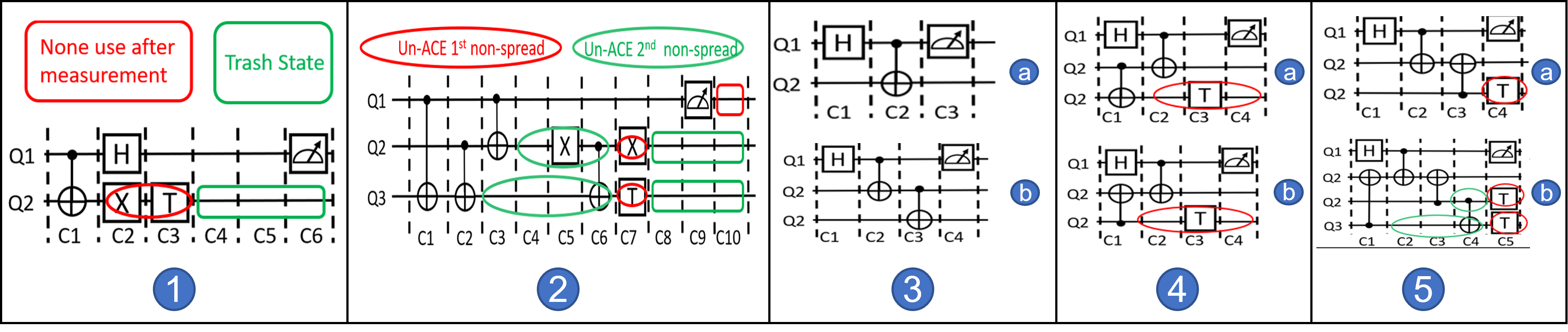
Case 1: Measurement logical qubit. This case contains outputting logical qubits that will be written to at least one of the output bits after measurement. The current examples shown in the paper will only have one measurement gate at the end of the circuit for a virtual qubit, and each of the measurements will be saved to one classical register. All the classical registers together form an output bit string. However, measuring on a specific virtual qubit multiple times is allowed as some algorithms require an intermediate result to control a controlled gate. Therefore, only the result will be used as a metric to determine the un-ACE status. Thus, some of the intermediate measurements will not act as an indicator. Being conservative, logical qubits in this case will largely remain in an ACE state. This is because the qubit is being measured, and an error in any earlier cycle can change the measured result. Therefore, it stays in the ACE state during the cycles between its initialization and measurement. There is still an opportunity to define un-ACE cycles for these logical measurement qubits, specifically where the quantum state it contains will not be needed. For example, the cycles before initialization and after the measurement with no remaining operation gates, which can be seen in Fig. 5.2 labeled as none used after measurement.

Case 2: Trashed state. If a logical qubit enters the trashed state, then that logical qubit enters the un-ACE state for all cycles until the end of the circuit. The prerequisite for being in the trashed state is that the logical qubit does not entangle with other qubits and stays idle without any computational operations for the rest of the circuit. Such a case can happen on assisting logical qubits and used ancilla qubits, with an example shown in Fig. 5.1-2. It is easy to prove the un-ACE property for the target qubit since any error that occurs in the trashed state cannot influence other qubits and its information is not measured, therefore errors will not affect the output.

Case 3: First-level non-spread logical qubit. When a logical qubit does not write its state to the output bits and there is still some single-qubit gate operating on it after the last CNOT gate, then the logical qubit enters the un-ACE state after the last CNOT gate. A simple example is shown in Fig. 5.1, which leaves $Q_{2}$ to become an un-ACE qubit starting from cycle 2. This can be verified by quantum states after the CNOT gate is no longer needed and transferred to others.

Case 4: Second-level non-spread logical qubit. After determining the first-level non-spread logical qubits and marking their cycles into un-ACE states, there is a unique situation where both operands of a CNOT gate are followed by an un-ACE state. Therefore, the CNOT operation for both logical qubits can also be in an un-ACE state. Then a second-level non-spread logical qubit can start to search the path for both logical qubits until reaching its next CNOT, a simple example shown in Fig 5.2. The second-level non-spread determination process can be performed multiple times to reach out to all the possible non-spread states with the upper limit for the number of searched cycles equal to the total cycle count.

5.3.2 Entangled Logical Qubit

When qubits become entangled, if one of the qubits is measured, then the other qubit will also instantaneously collapse to a predefined state based on the structure of the entanglement. Therefore, before the entanglement is terminated either by measurement or inserting specific gates, an error in one logical qubit does not require a CNOT gate to propagate. Consequently, when determining the un-ACE qubit states, entanglement and CNOT gate paths should be considered simultaneously.

Entangled logical qubits. In the circuit shown above in Fig. 5.3.a-b, the two logical qubits form a Bell state, which is one way to create entanglement [23]. Since $Q_{1}$ has a measurement that belongs to outputting logical qubit group, both $Q_{1}$ and $Q_{2}$ will stay in ACE states for the entire circuit. Errors that occur at any cycle could be transferred to the output. In Fig. 5.3.b, we demonstrate one way to create an entanglement qubit group with more than two qubits, which also remains ACE for all cycles.

Logical qubit operating with entanglement qubits. As shown in Figs. 5.4.a-b and 5.5.a, we have demonstrated cases where an assisting logical qubit could have un-ACE states when involved in CNOT operations with entangled qubits. Those three cases plus the case in 5.3.b illustrate all the possible CNOT gate interactions between an assisting logical qubit and entangled qubit pairs involving at least one outputting logical qubit. We can entangle the third qubit only after successfully creating a Bell state and targeting the third qubit with a CNOT operation. The entanglement created from more than two qubits forms the GHZ states [12] which follows the same relation as discussed.

In those sub-figures that fail to entangle the third qubit, we can identify un-ACE states for the third logical qubit. For Fig 5.4.a, even if $Q_{3}$ serves as the target for the CNOT operation, its phase state will pass to $Q_{2}$, known as the phase-kickback phenomenon [2]. That is the reason we cannot list $Q_{3}$’s cycles before the CNOT gate as the un-ACE state.

As illustrated in Fig. 5.5.b, assisting logical qubits can also be classified into the secondary non-spread state. However, a careful examination of the additional logical qubit’s entanglement status should be considered.

6 Computing QVF and CQV

When computing the AVF for classical computers, Little’s Law and Performances Model [18] are the primary candidates to make a low-cost estimation of the ACE bits for a given hardware structure based on un-ACE instructions. However, we cannot perform such analysis when computing QVF because we do not have instructions (such as no-ops or mask instructions) where we can determine specific un-ACE bits. From the last section’s analysis, we have not found any distinct instruction from which we can identify the un-ACE qubit states.

For computing the QVF for a given circuit on a specific chip, information on the entire final circuit is required since any missing cycles could lead to possible error propagation paths. Moreover, even though the compiler can merge subcircuits to generate a new total circuit for solving sophisticated quantum algorithms, the QVF for the subcircuits may not be used to compute the total QVF. There are cases where a logical qubit identified as an un-ACE qubit state in one subcircuit might be used again when combined with other subcircuits, changing the ACE status of that qubit. These later-used states will conflict with the prior defined un-ACE states. Therefore, it is recommended to perform the QVF determination procedure every time after creating a new final circuit.

The equation for computing the QVF of a given chip running a specific benchmark is simply the average QVF for all the ACE states on the chip for a given cycle. Such QVF at cycle $C_{t}$ can be written as:

$$QVF\_C_{t}=\frac{\sum_{ACE\ States\ at\ C_{t}}\ Calibrated\ Error\ Rate}{Device\ physical\ qubit\ count\ }\$$ (4)

Based on this, the QVF for a quantum chip shows the average QVF for the entire circuit, which can be written as:

$$QVF=\frac{\sum_{cycles}\sum_{ACE\ States}\ Calibrated\ Error\ Rate}{Number\ of\ physical\ qubits\times total\ cycles}\$$ (5)

It is common for small algorithms to use many ancilla qubits that stay in the unused case as the algorithm does not require many qubits. For these cases, we propose the Used QVF (UQVF) which only considers the virtual qubits used.

Since QVF is designed to present the average FR of quantum execution at the cycle level, we also propose the Cumulative Quantum Vulnerability (CQV) to present the final circuit’s vulnerability by predicting the FR for the compiled circuit. To be clear, the CQV will not predict the correct result but the possibility of not receiving a correct result when repeating execution. In contrast, $1-CQV$ represents the estimated success rate driven by using the CQV model. To compute the CQV, we build a Monte Carlo simulator based on the QVF model to predict the value of $1-CQV$.

The simulator iterates through the compiled circuit for each physical qubit in every cycle. If the physical qubit in question is in the ACE state, the cumulative success rate of the corresponding virtual qubit will be updated by multiplying the running success rate with the gate success rate calculated in equation 2. We perform a crosstalk error calibration based on [22] and update the gate success rate of the victim by multiplying it with the calibrated crosstalk gate success rate. If the targeting operation is a CNOT gate, then the error from its paired qubit will also be affecting the target qubit. For all such cases in a given compiled circuit, we propose a weight, ranging from 0 to 1, to represent the portion of cumulative errors, one minus the corresponding accumulative success rate, which could flow across the CNOT gate. Then the accumulating success rate of such testing qubit will multiply with both the CNOT gate success rate and the Success Rate from its paired virtual qubit determined by only using the weight portion of the cumulative error. A heuristic method to provide a proper weight selection for a given compiled circuit is discussed in detail in Section 7. In the end, the value of $1-CQV$ is determined by multiplying the final cumulative success rates of all the outputting logical qubits.

7 Determining Weight

Now that we have designed the error model, we will analyze the weight, one of the major coefficients in the CQV calculation. We ultimately identify a method to choose a proper weight for CQV to provide an accurate prediction for the real success rate at compile time.

7.1 Is the Weight Trivial?

Before identifying the value of the weight, we first demonstrate the prediction performance when the weight is set equal to zero or one representing no error or full error crossover the CNOT gate, respectively. The compiled circuits of the experiments are generated from different combinations of compiler settings for all four benchmarks at both algorithm sizes. The CQV calculation is performed using the calibration error and execution results from IBMQ_Montreal on Apr. 1st 2022. As shown in Fig. 6, though the $1-CQV\_0$ results are closer to the real success rate than ESP, there are still noticeable differences between $1-CQV\_0$ and the real SR which means some errors are not being well represented. Meanwhile, $1-CQV\_1$ makes predictions close to zero all the time and loses track of the real SR, meaning the errors are being overestimated. The experiment results show that, for those benchmarks, using zero or one as the weight will lead to inaccurate predictions.

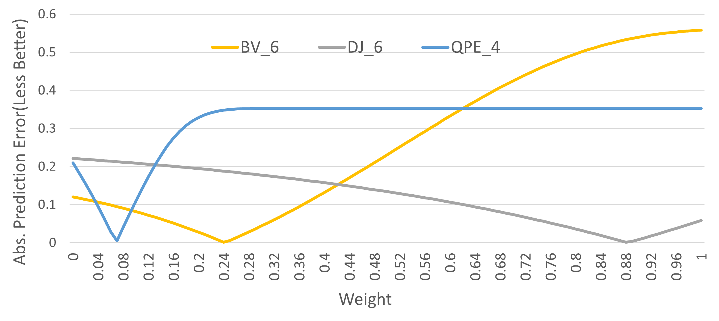
Since assigning the weight as zero or one for those benchmarks is not accurate, we would want to know the relationship between weight and prediction accuracy. As shown in Fig. 7, by plotting the absolute prediction error with all the weights with 1% granularity, we can identify which weight achieves the lowest prediction error compared to all the other weights. We also calculated the correlation between the weight value and its corresponding 1-CQV prediction, and all three correlations are approximate to -1, which is consistent with the relationship in Fig. 7.

Figure 6: Average Success Rate Prediction Comparison Between Weight as 0 and 1 for benchmarks on IBMQ_Montreal

7.2 Determine a Proper Weight

After knowing that the best weight should be a number between zero and one, how can we approximate it at compile time to assist the CQV calculation in predicting the real success rate? To answer that question, we propose a heuristic method that first calibrates the best weights among different compiled circuits on a target machine and then uses a heuristic function generated from the calibration data to locate a proper weight.

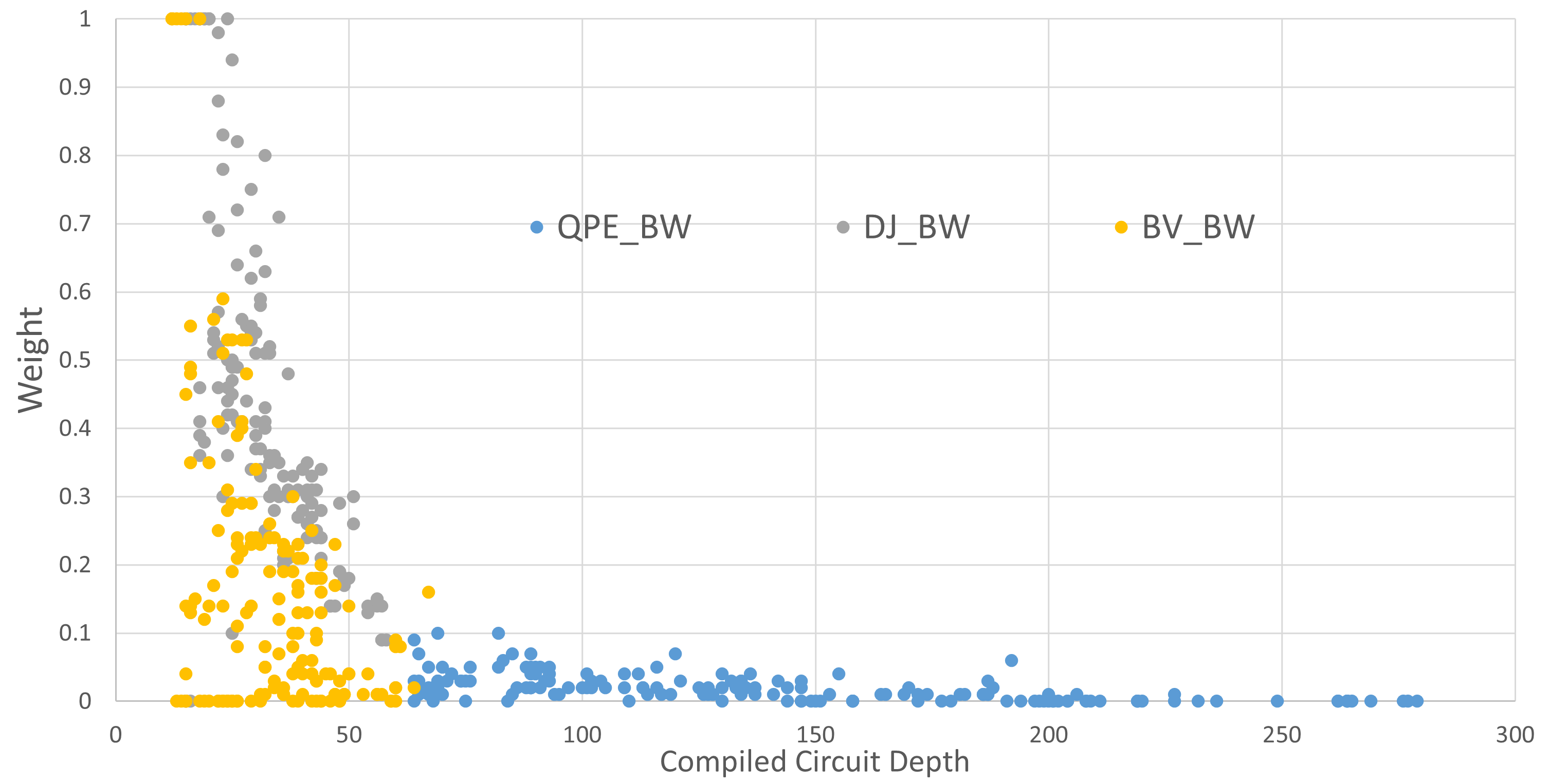
The first step of the calibration process is to execute many compiled circuits generated from target benchmarks with various compile strategies on the target quantum machine. The two prerequisites for choosing a target benchmark are that the benchmark has only one correct output and that the correct output can be determined to calculate the real SR. After getting the real SRs, the second step of the calibration process will provide the full spectrum of weights for the CQV calculation and determine the best weight for each compiled circuit using the same method as in Fig. 7. As shown in Fig. 8, we have plotted the best weight against the depth of the compiled circuit. The result is consistent with our expectation – the best weight will be very arbitrary when the depth is short, but as the depth of the compiled circuit increases, the best weight begins to converge and shows an overall decreasing trend.

Here, we give a short analysis of the best weight distribution. By checking the experiment data, we find out that, the SR of these benchmarks will drop to less than 10% when their depth is greater than 100 and less than one percent when the depth is greater than 150 cycles, accordingly. Furthermore, if the depth is greater than 150 cycles, the best weight tends to approach zero. A possible explanation behind this would be that, as the depth increases, the quantum states tend to mix more, which possibly decreases on average the effect of errors. Another possibility might be that errors may cancel to some degree. Since the vulnerability model we use treats any operation error on an ACE qubit as a sign that will lead to incorrect output. However, in the real operating environment, later errors could adjust the previous error in the dynamic noise system, causing the original wrong quantum state to return closer to the correct state. At the same time, since noise would cause almost every possible output result to appear for certain trials, certain correct trials may be caused by noise as well. These two low-probability cases will stand out as the SR of a benchmark decrease, especially when the SR stays between 10% and 0.1%. Ultimately, with a very deep circuit, the best weight will decrease even more to accommodate for such small probability cases due to fewer correct trials.

The second step of the heuristic method is to use a heuristic function to determine the proper weight for a given compiled circuit. The heuristic function used in this paper is the logarithmic average of all the best weights within the target depth section according to the data in Fig. 8.

To predict a compiled circuit on a target machine, one can calculate the CQV based on the weight captured by either repeating our full heuristic process or using the heuristic function to choose weight based on our calibrated data in Fig. 8. Starting from now, our heuristic method will be the default way to find the weight used in CQV calculations. Please notice that our heuristic method of choosing the weight is designed to accommodate any hardware upgrades.

Figure 7: Capture the best weight for benchmarks with 1% steps

Figure 8: Comparing the Best Weight among all experiments

8 Implementation

We use Qiskit [14], an open-source framework for quantum computing, to evaluate our QVF determination process. We augment Qiskit version 0.34.2, which performs the QVF and CQV calculations based on the executable final circuit called the transpiled circuit or compiled circuit. We implement four functions to perform the simplified QVF calculation workflow as shown in Fig. 9.a.

Figure 9: Complete QVF and CQV process and circuit booking example

Table 2: Benchmarks and Quantum Chips Description

Item	Description
Bernstein-Vazirani (BV)	contain assisting logical
	qubit
Deutsch-Jozsa (DJ)	contain assisting logical
	qubit
Quantum Fourier Transform	no assisting logical qubit
(QFT)
Quantum Phase Estimation	no assisting logical qubit
(QPE)
ibmq_montreal	27-qubits with Hexagon
ibmq_toronto	27-qubits with Hexagon
ibmq_mumbai	27-qubits with Hexagon
ibmq_brooklyn	65-qubits with Hexagon

Entanglement Finder. Determining the entanglement relationships among the qubits in the circuit is critical for performing an accurate un-ACE state analysis and thus the later QVF calculation, though detecting entanglement in a quantum system is one of the active research fields with no simple solutions [4, 27]. For our design, there are two ways to identify the entangled qubits and their entangled cycles. The first method requires the software engineer who builds the logical qubits to input the designated entangled qubits and their entanglement durations. The second method will do a brute-force search to locate all Bell states and GHZ states from the logical circuit. For now, Bell states and GHZ states are the only two entangled states our entanglement finder can identify.

Circuit Booking. At this step, the circuit booking function will receive a list of entangled qubits with the information of their entangled virtual qubit names and the start cycles and end cycles of their entanglement. The final compiled circuit is also sent to the circuit booking function, which builds a table based on this final circuit. The rows are the physical qubits, and the columns are the cycle index. Each cell contains some variables of the circuit. An example of the output table generated by the circuit booking function is shown in Fig. 9b, which presents all the variables for the cell with indices below them. The first variable is the name of the virtual qubit the current physical qubit holds at this cycle. The next variable contains the entanglement information of the virtual qubits. If not empty, the second variable presents the name of the virtual qubit it entangled with. If entangled among more than 2 qubits, to reduce conflict, all the others in the entanglement will write the first entanglement qubit in the second index. The third variable holds S if it belongs to an intermediate process of a swap gate. The fourth index represents O if the virtual qubit is an outputting logical qubit. The last variable represents the ACE status of the virtual qubit at such a cycle.

Identifying Un-ACE Cases. This function takes the table generated by the circuit booking function and determines the un-ACE status from the final circuit which changes the table’s ACE status variable. The determination will run over all the physical qubits starting from the last cycle to the first cycle. The first iteration will determine the virtual qubit’s ACE status variable based on the status of the outputting logical qubit variable and entanglement information variable in this cycle. The inspection will go over all the cases listed in section 4 and perform the search until it exhausts all the second-level non-spread cases.

Calculating QVF and CQV. This function will calculate the QVF and CQV based on the table’s ACE variable modified by the last function. The equations and processes for generating those numbers are listed in section 6.

Table 2 is the description of the backend and benchmark used in our evaluation. We run our experiments on state-of-the-art quantum machines with 27 and 65 qubits. The description column lists the information of the quantum chip, with qubit size and its connecting shape.

9 Results

9.1 CQV Accuracy

Algorithm size within Quantum Volume In this section, we will present the CQV prediction performance for BV, DJ, and QPE benchmarks on the three 27-qubit machines IBMQ_Montreal, IBMQ_Toronto, and IBMQ_Mumbai with weights calculated from the Apr. 1st error calibrations. As shown in Figure 10, we present the 1-CQV prediction accuracy compared with ESP for QPE with varying compiled circuits on IBMQ_Montreal on Apr. 5th. The different configurations are guidelines for the compiler to generate the final compiled circuit based on the given logical circuit and target device. The configurations used in Figure 10 are generated for all the three algorithm sizes (4, 5, and 6 qubits) of the QPE benchmark. The first integer of the configuration lists the size of the algorithm. The second integer ranging from 0 to 2 indicates the optimization level used in the configuration, which implements different optimization steps. The next variable illustrates the layout method used, which corresponds to different qubit allocation strategies. The last variable describes the routing method used, which directs qubit movement. By following different configurations, Qiskit will generate different compiled circuits based on the same QPE logical circuit with the same number of qubits, which is used to generate many different inputs for our experiments showing the accuracy of the quantum SR estimators. The blue bar indicates the real success rate after executing each configuration. The grey and blue bar indicate our success rate prediction driven from $1-CQV$ and the ESP prediction, respectively. The closer to the blue bar, the more accurate the prediction. It is clear that $1-CQV$ is much closer to the real SR compared to the ESP. After shown to the right of Fig. 10, the average absolute error rate for ESP over all the configurations compared to ground truth SR is 37%, while $1-CQV$ achieves an average error of 4%. Such an error rate difference means that $1-CQV$ achieves a 94% error reduction compared to the ESP, which also means the CQV calculation is adaptable to the variation errors in different calibration periods and provides excellent predictions.

By inspecting Fig. 10, SR drops clearly when the algorithm size increases, which follows the nature of the benchmark by employing significantly more two-qubit gates. When increasing algorithm size, not only does the number of two-qubit gates increase, but the number of swapping operations also increases.

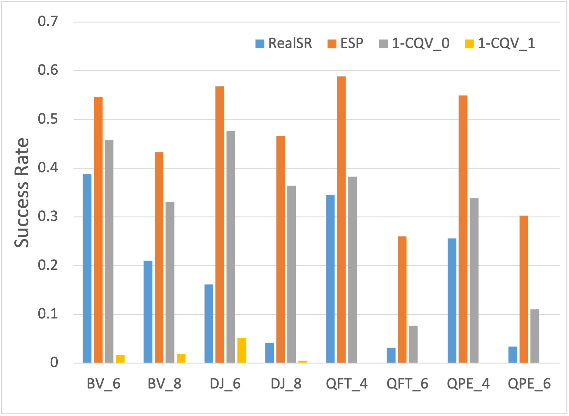
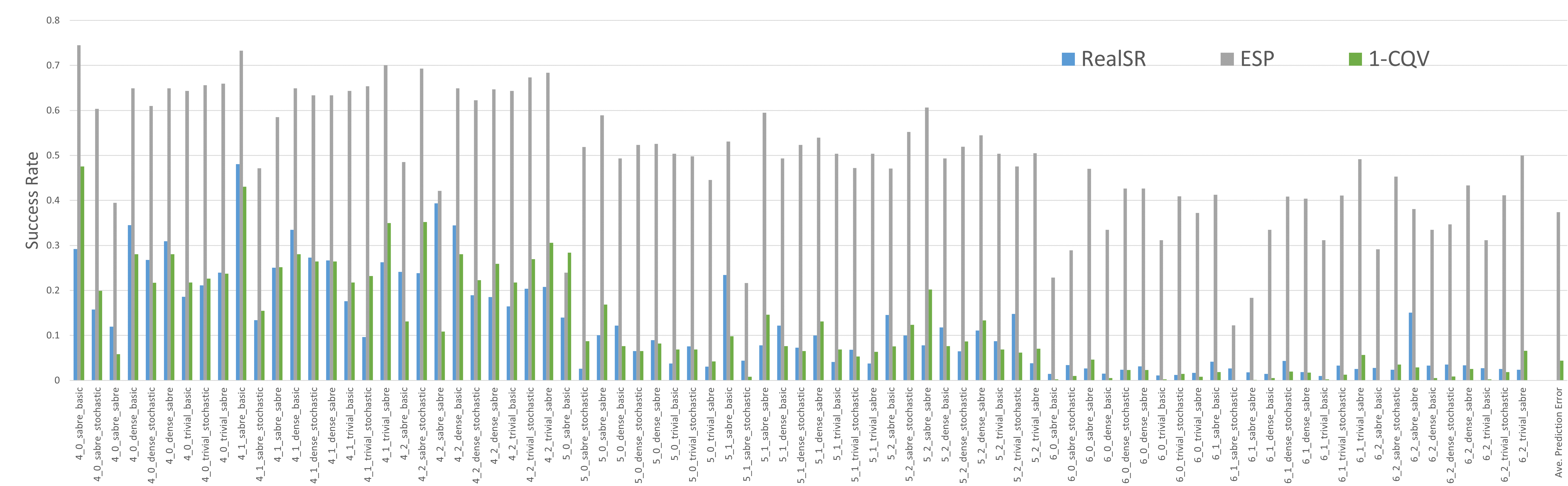
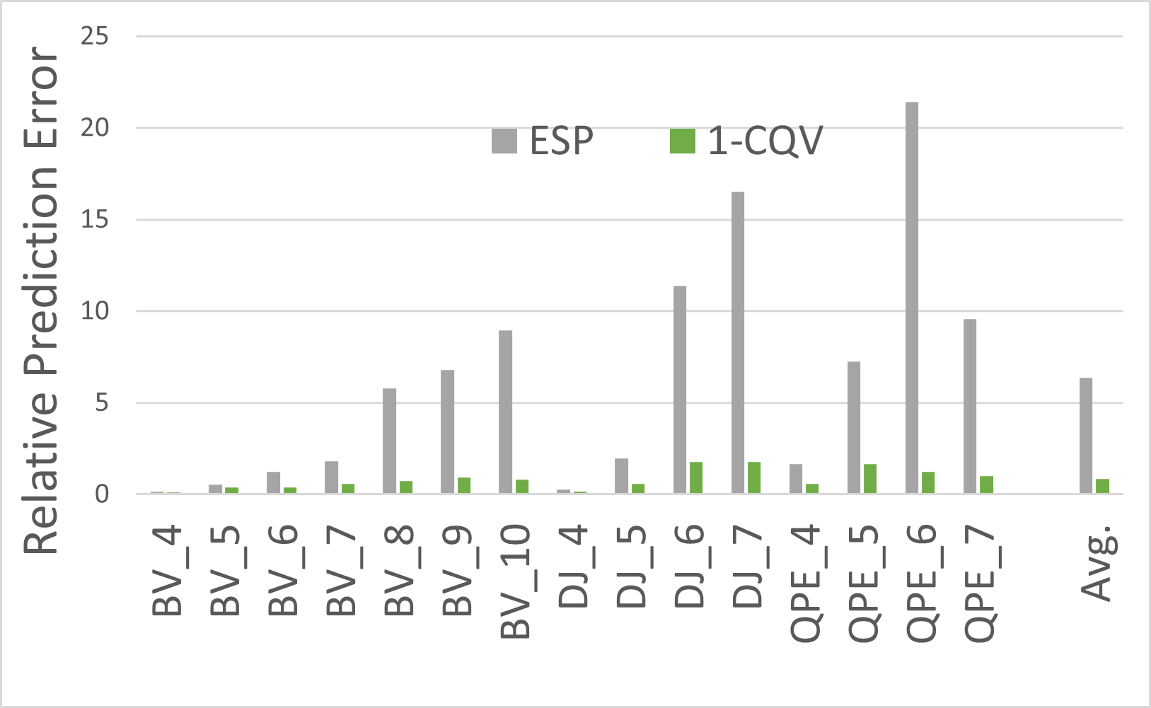
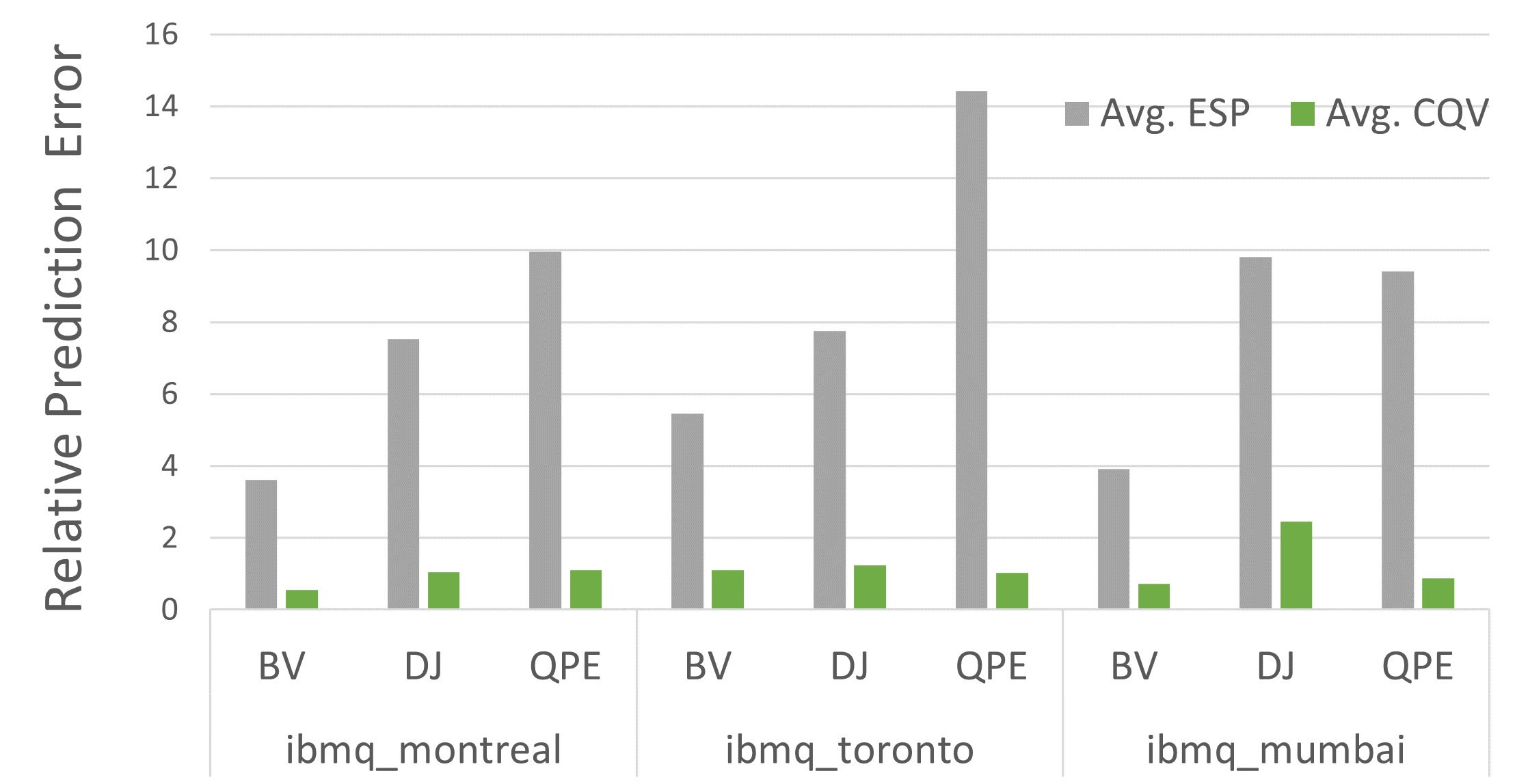
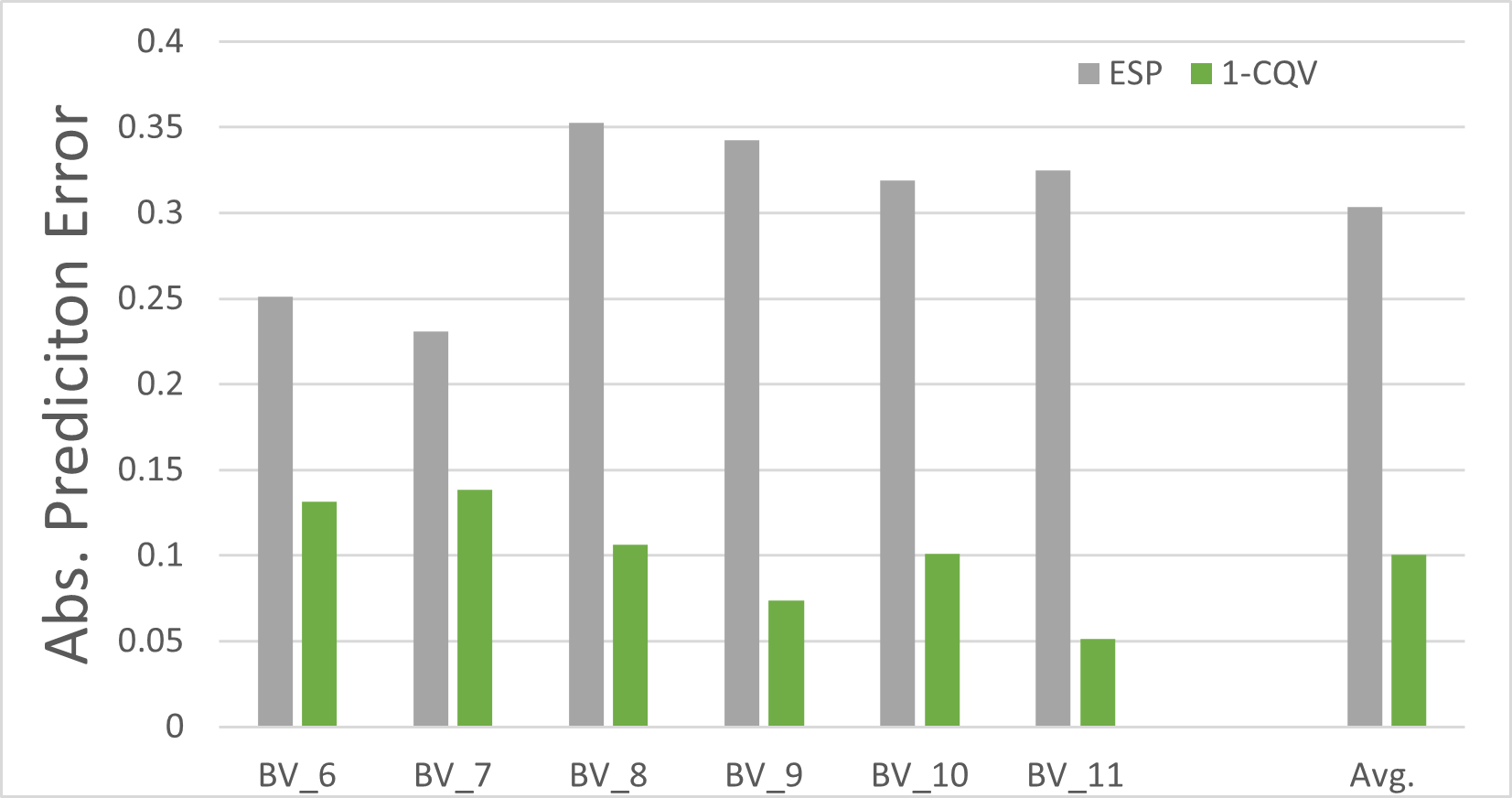
As shown in Fig. 11, we present the 1-CQV prediction for all the benchmarks on the single machine IBMQ_Montreal at Apr. 8th. In the figure, we include experiments with an SR higher than 0.1%. The relative prediction error is a metric produced by dividing the absolute prediction error by the SR. From the figure, it is easy to find that the 1-CQV prediction outperforms the ESP by achieving an average of 6 times and best at 20 times less relative prediction error rate. As shown in Fig. 12, 1-CQV presents a stable and accurate average relative prediction error across all machines and benchmarks with data collected on Apr. 9th.

When calculating CQV, our simulator takes the two-qubit gates into account and considers the influence of both qubits’ accumulated success rates. From these observations, we can say that the CQV has better error modeling than the ESP noise model.

Figure 10: Predicted and real success rates of QPE with IBMQ$\_$Montreal Quantum machine 4/5/22

Algorithm size beyond Quantum Volume

From the results shown in Fig. 10, 11, 12, it is surprising that the $1-CQV$ has an accurate and stable prediction of the real success rate even when it falls in the 10% to 0.1% range, which was ignored in previous research. The major reason for the low success rate is that the size of the compiled circuits equals or exceeds the desired quantum volume of the target quantum machine. The simple explanation of quantum volume could be the product of virtual qubits and circuit depth. Such observation leads to a conclusion that the $1-CQV$ prediction is accurate across the full spectrum of algorithm sizes and success rates.

After making a full spectrum comparison among all the backends and benchmarks, from the observations of the results, we can say that the CQV has better error modeling than the ESP noise model.

Figure 11: Average relative predict error for all the benchmarks on single Quantum machine IBMQ_Montreal

Figure 12: Average relative predict error across all benchmarks and backends

As shown in Fig. 11, we have demonstrated the CQV prediction is stable across different algorithms on single machines, and the result shows that CQV has an overall stable and less relative error rate and performs much better when the algorithm reaching and passing the quantum volume.

9.2 Scalability Analysis of CQV

We performed the scalability analysis of the CQV in this section by reporting the execution time. We chose to test QFT with input sizes varying from 5 to 120 using the fake backend of IMBQ_Washington with 127-qubits. Instead of focusing on the predicted result which should be close to zero when getting too large, we are interested in the execution time of different prediction methods. As shown in Table 3, it is clear that the execution time of CQV scales linearly with the CX gate count, which would provide reliable scalability to help future quantum research.

Table 3: Quantum Estimator Scalability Comparison(Second)

Algorithm	CX count	ESP	Qiskit	CQV
QFT_5	59	0.00299	1.31142	0.00700
QFT_10	408	0.02004	1.86264	0.03100
QFT_15	1383	0.06101	N/A	0.15903
QFT_20	2657	0.09802	N/A	0.22605
QFT_50	26408	0.71115	N/A	5.97225
QFT_100	157428	1.83842	N/A	7.76095
QFT_120	208260	3.10630	N/A	20.3832

9.3 Weight Sensitivity Study

Figure 13: Weight stable Study for different weight settings for a week on IBMQ_Montreal

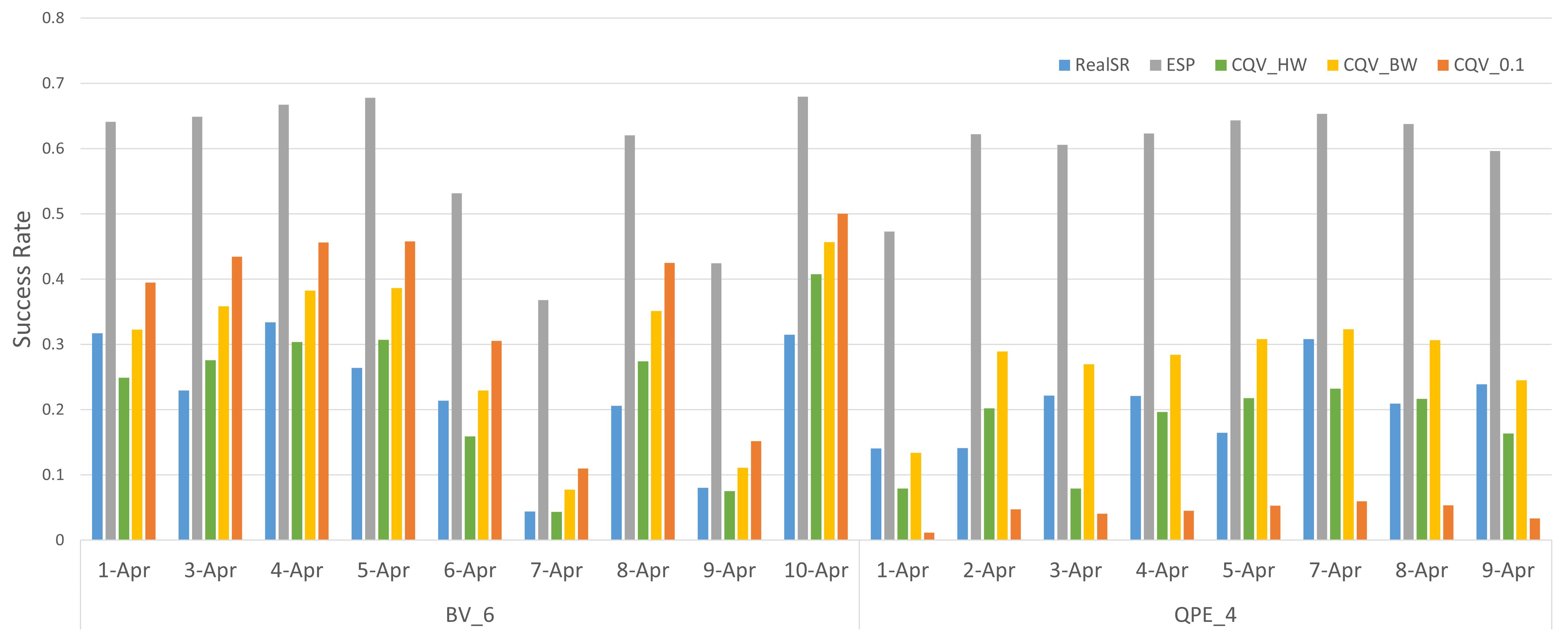
The goal of this subsection is to understand whether the prediction accuracy of CQV will be subject to the volatile nature of current NISQ quantum machines’ error rates and whether the best weight predictions for a certain day will remain optimal for the same experiment in the future. We performed two repeated experiments for more than a week and presented the CQV with various weight settings in Fig. 13. Both experiments are chosen because the best weights of the experiments found on April 1st are not equal to the weights determined by the heuristic method. For CQV_HW and CQV_BW, the experiments on different dates used the same weight determined on the Apr. 1st, respectively. As shown in Fig. 13, starting from Apr. 3rd, the CQV_HW presents less prediction error for seven out of eight times compared to the CQV_BW using the best weight of Apr. 1st. For QPE_4, the CQV_HW is more accurate than CQV_BW four out of seven times when predicting the SR. The CQV_0.1 is representing the weight as 10% which is a simple and quick way to perform prediction without the need to make the weight calibration in advance. It is clear that the heuristic weight is stable enough to provide accurate prediction against noise variations over days and the best weight for one compile configuration might change over days. After inspecting those experimental results, we found out that the machine was later reporting partially disabled functionality, such as certain CX gates having a 100% error rate. Those dates’ results were ignored and left gaps in the date axis.

10 Case Study

10.1 Case 1: Unseen Benchmark

In the previous section, we demonstrated that - at compile-time, CQV could make an accurate prediction for algorithms on machines that have been previously used to determine the weight. In this section, we will explore the predictive power of CQV to estimate real SR for unseen algorithms and then unseen machines.

We choose the QFT algorithm as the unseen algorithm. The QFT has been widely used as a building block for other algorithms and is also used to form part of the QPE algorithm. To decrease the association between the QPE and QFT, we generate the QFT benchmarks inversely compared to its counterpart in QPE. The weight for each machine was chosen based on the heuristic method illustrated in Sec. 7.2 using the other three algorithms, accordingly. As shown in Table 4, we have presented the detailed CQV prediction performance of QFT on all three machines. The CQV result is surprisingly accurate with an average of 3% absolute prediction error across all machines and algorithm sizes. The algorithm also achieves at least 6 times less average relative prediction error for CQV compared to the ESP. The 0.41 average relative prediction error of 1-CQV across all the machines and algorithm size supports that the CQV could be used as a stable and accurate SR estimator for unseen algorithms.

10.2 Case 2: Unseen Machine

Figure 14: Average abs. predict error of BV on unseen IBMQ_Brooklyn

Table 4: CQV Prediction for Unseen Algorithm QFT

2022_04_12			Avg. Prediciotn		Avg. Abs. Prediciotn Error		Avg. Relative Prediction Error
Machine	Benchmark	RealSR	ESP	1-CQV	ESP	1-CQV	ESP	1-CQV
ibmq_montreal	QFT_4	0.340843	0.643122	0.298255	0.302279	0.04258817	0.886858	0.124949565
	QFT_5	0.129277	0.522711	0.122285	0.393434	0.00699177	3.043343	0.054083654
	QFT_6	0.028583	0.289672	0.006614	0.261089	0.0219689	9.134565	0.768612629
ibmq_mumbai	QFT_4	0.173173	0.585265	0.241069	0.412092	0.06789655	2.379662	0.392074505
	QFT_5	0.056254	0.437791	0.081249	0.381537	0.02499528	6.782389	0.444328395
	QFT_6	0.032936	0.272236	0.009243	0.2393	0.02369366	7.265511	0.719376703
ibmq_toronto	QFT_4	0.212094	0.571954	0.254039	0.359861	0.04194556	1.696706	0.197769098
	QFT_5	0.070116	0.426818	0.084775	0.356702	0.01465873	5.087331	0.209064487
	QFT_6	0.032585	0.250512	0.006355	0.217926	0.02622974	6.687909	0.804960147

One of the challenges the current quantum researchers face is lack of the access to physical machines, which impacts the validation of their design. Therefore, performing the full heuristic method to determine the corresponding weight could not be done on a machine without access. In such a scenario, one can use the weight calibrations from other machines to perform the CQV prediction with a seen benchmark on the unseen machine at compile time. We have performed such an experiment and validated the CQV by comparing it with the real SR. As shown in 14, we used the machine IBMQ_Brooklyn to represent the unseen machine with weight calibrated from IBMQ_Montreal. Due to the limited QV of IBMQ_Brooklyn, BV is the only benchmark that is completed without reporting errors. The 1-CQV achieves an average 10% absolute prediction across all the algorithm sizes. Though such prediction error is two times higher than the corresponding prediction of BV on IBMQ_Montreal, it still outperforms the ESP by three times. The IBMQ_Montreal has 27 qubits and IBMQ_Brooklyn has 65 qubits, which could be the reason for less accurate prediction. If 10% average prediction accuracy is suitable for the validation, then CQV would help to make predictions on the unseen machines.

11 Related Work

The early research on quantum computing was focused on designing quantum instruction set architecture [7] and quantum computer microarchitecture [9, 8, 20, 21] for solving the constraints to apply logical circuits to machines. After that, the temporal and spatial noise variation problems of superconducting quantum computers have been discovered and studied in [34, 19], which also provide mapping and allocation-enhanced compilations based on such variations. Currently, the focus of quantum computing is on optimizing the success rate by applying different compiler strategies, such as mitigating the effect of errors by enhancing the quantum instructions [28, 11], decreasing measurement errors [33, 10], mitigating crosstalk errors [22, 5], combining the mappings to reduce dissimilar mistakes [32], and compiling with specific constraints [16, 5]. Although fault paths within quantum circuits have been studied to trace error propagation[15], such a method requires the Clifford-gate error rates which are not available in the current quantum computers. Quantum fault injection [26] is also being studied but fails to scale up due to the exponential growth requirement on computation power. Though ESP mode created in [24] is widely used as a lightweight success rate predictor, such method sufferers from low prediction accuracy and high relative error rate while increasing algorithm size. To the best of our knowledge, there is no prior work that provides a systematic approach to determining all ACE cases and adding such information to each gate on whether the error will result in fault output. In addition, based on the QVF model, this work provides a CQV metric to provide accurate FR.

ACE analysis [17, 18], architectural vulnerability factor (AVF) prediction [35, 6], and program vulnerability factor (PVF) [30] estimation have been well studied for conventional computer systems. This work is inspired by the prior research in conventional computers but performs a different ACE analysis procedure for quantum computers during the compilation stage instead of at runtime.

12 Conclusion

In conclusion, inspired by AVF our paper proposes QVF to quantify the average ACE states of a chip at any given cycle, which can present the circuit and noise behavior. Based on the QVF, we propose the CQV metrics to predict the failure rate of a given compiled circuit. By validating our design on state-of-the-art quantum machines with well-known benchmarks, in both seen and partially unseen systems, we have achieved an average of 6 times less relative prediction error rate compared to the state-of-the-art SR estimator ESP, which can assist and speed up the quantum computing research at both the hardware and software levels.

References

- [1] J. Clarke and F. K. Wilhelm, “Superconducting quantum bits,” Nature, vol. 453, no. 7198, pp. 1031–1042, 2008.
- [2] R. Cleve, A. Ekert, C. Macchiavello, and M. Mosca, “Quantum algorithms revisited,” Proceedings of the Royal Society of London. Series A: Mathematical, Physical and Engineering Sciences, vol. 454, no. 1969, pp. 339–354, 1998.
- [3] L. DiCarlo, J. M. Chow, J. M. Gambetta, L. S. Bishop, B. R. Johnson, D. Schuster, J. Majer, A. Blais, L. Frunzio, S. Girvin et al., “Demonstration of two-qubit algorithms with a superconducting quantum processor,” Nature, vol. 460, no. 7252, pp. 240–244, 2009.
- [4] A. Dimić and B. Dakić, “Single-copy entanglement detection,” npj Quantum Information, vol. 4, no. 1, pp. 1–8, 2018.
- [5] Y. Ding, P. Gokhale, S. F. Lin, R. Rines, T. Propson, and F. T. Chong, “Systematic crosstalk mitigation for superconducting qubits via frequency-aware compilation,” in 2020 53rd Annual IEEE/ACM International Symposium on Microarchitecture (MICRO). IEEE, 2020, pp. 201–214.
- [6] L. Duan, B. Li, and L. Peng, “Versatile prediction and fast estimation of architectural vulnerability factor from processor performance metrics,” in 2009 IEEE 15th International Symposium on High Performance Computer Architecture. IEEE, 2009, pp. 129–140.
- [7] X. Fu, L. Riesebos, M. Rol, J. van Straten, J. Van Someren, N. Khammassi, I. Ashraf, R. Vermeulen, V. Newsum, K. Loh, J. C. de Sterke, W. J. Vlothuizen, R. N. Schouten, C. G. Almudever, L. DiCarlo, and K. Bertels, “eqasm: An executable quantum instruction set architecture,” in 2019 IEEE International Symposium on High Performance Computer Architecture (HPCA). IEEE, 2019, pp. 224–237.
- [8] X. Fu, M. Rol, C. Bultink, J. van Someren, N. Khammassi, I. Ashraf, R. Vermeulen, J. de Sterke, W. Vlothuizen, R. Schouten, L. DiCarlo, and K. Bertels, “A microarchitecture for a superconducting quantum processor,” IEEE Micro, vol. 38, no. 3, pp. 40–47, 2018.
- [9] X. Fu, M. A. Rol, C. C. Bultink, J. Van Someren, N. Khammassi, I. Ashraf, R. Vermeulen, J. De Sterke, W. Vlothuizen, R. Schouten, C. G. Almudever, L. DiCarlo, and K. Bertels, “An experimental microarchitecture for a superconducting quantum processor,” in Proceedings of the 50th Annual IEEE/ACM International Symposium on Microarchitecture, 2017, pp. 813–825.
- [10] P. Gokhale, O. Angiuli, Y. Ding, K. Gui, T. Tomesh, M. Suchara, M. Martonosi, and F. T. Chong, “Optimization of simultaneous measurement for variational quantum eigensolver applications,” in 2020 IEEE International Conference on Quantum Computing and Engineering (QCE). IEEE, 2020, pp. 379–390.
- [11] P. Gokhale, A. Javadi-Abhari, N. Earnest, Y. Shi, and F. T. Chong, “Optimized quantum compilation for near-term algorithms with openpulse,” in 2020 53rd Annual IEEE/ACM International Symposium on Microarchitecture (MICRO). IEEE, 2020, pp. 186–200.
- [12] D. M. Greenberger, M. A. Horne, and A. Zeilinger, “Bell’s theorem, quantum theory, and conceptions of the universe,” 1989.
- [13] IBM, “Ibm quantum,” https://quantum-computing.ibm.com/, retrieved on 04-16-2021.
- [14] IBM, “Open-source quantum development,” https://qiskit.org/, retrieved on 04-16-2021.
- [15] S. Janardan, Y. Tomita, M. Gutiérrez, and K. R. Brown, “Analytical error analysis of clifford gates by the fault-path tracer method,” Quantum Information Processing, vol. 15, no. 8, pp. 3065–3079, 2016.
- [16] G. Li, Y. Ding, and Y. Xie, “Tackling the qubit mapping problem for nisq-era quantum devices,” in Proceedings of the Twenty-Fourth International Conference on Architectural Support for Programming Languages and Operating Systems, 2019, pp. 1001–1014.
- [17] S. Mukherjee, C. Weaver, J. Emer, S. Reinhardt, and T. Austin, “A systematic methodology to compute the architectural vulnerability factors for a high-performance microprocessor,” in Proceedings. 36th, 2003.
- [18] S. S. Mukherjee, J. Emer, and S. K. Reinhardt, “The soft error problem: An architectural perspective,” in 11th International Symposium on High-Performance Computer Architecture. IEEE, 2005, pp. 243–247.
- [19] P. Murali, J. M. Baker, A. Javadi-Abhari, F. T. Chong, and M. Martonosi, “Noise-adaptive compiler mappings for noisy intermediate-scale quantum computers,” in Proceedings of the Twenty-Fourth International Conference on Architectural Support for Programming Languages and Operating Systems, 2019, pp. 1015–1029.
- [20] P. Murali, N. M. Linke, M. Martonosi, A. J. Abhari, N. H. Nguyen, and C. H. Alderete, “Architecting noisy intermediate-scale quantum computers: A real-system study,” IEEE Micro, vol. 40, no. 3, pp. 73–80, 2020.
- [21] P. Murali, N. M. Linke, M. Martonosi, A. J. Abhari, N. H. Nguyen, and C. H. Alderete, “Full-stack, real-system quantum computer studies: Architectural comparisons and design insights,” in 2019 ACM/IEEE 46th Annual International Symposium on Computer Architecture (ISCA). IEEE, 2019, pp. 527–540.
- [22] P. Murali, D. C. McKay, M. Martonosi, and A. Javadi-Abhari, “Software mitigation of crosstalk on noisy intermediate-scale quantum computers,” in Proceedings of the Twenty-Fifth International Conference on Architectural Support for Programming Languages and Operating Systems, 2020, pp. 1001–1016.
- [23] M. A. Nielsen and I. Chuang, “Quantum computation and quantum information,” 2002.
- [24] S. Nishio, Y. Pan, T. Satoh, H. Amano, and R. V. Meter, “Extracting success from ibm’s 20-qubit machines using error-aware compilation,” ACM Journal on Emerging Technologies in Computing Systems (JETC), vol. 16, no. 3, pp. 1–25, 2020.
- [25] J. Preskill, “Quantum computing in the nisq era and beyond,” Quantum, vol. 2, p. 79, 2018.
- [26] S. Resch, S. Tannu, U. R. Karpuzcu, and M. Qureshi, “A day in the life of a quantum error,” IEEE Computer Architecture Letters, vol. 20, no. 1, pp. 13–16, 2020.
- [27] V. Saggio, A. Dimić, C. Greganti, L. A. Rozema, P. Walther, and B. Dakić, “Experimental few-copy multipartite entanglement detection,” Nature physics, vol. 15, no. 9, pp. 935–940, 2019.
- [28] Y. Shi, N. Leung, P. Gokhale, Z. Rossi, D. I. Schuster, H. Hoffmann, and F. T. Chong, “Optimized compilation of aggregated instructions for realistic quantum computers,” in Proceedings of the Twenty-Fourth International Conference on Architectural Support for Programming Languages and Operating Systems, 2019, pp. 1031–1044.
- [29] D. Solenov, J. Brieler, and J. F. Scherrer, “The potential of quantum computing and machine learning to advance clinical research and change the practice of medicine,” Missouri medicine, vol. 115, no. 5, p. 463, 2018.
- [30] V. Sridharan and D. R. Kaeli, “Eliminating microarchitectural dependency from architectural vulnerability,” in 2009 IEEE 15th International Symposium on High Performance Computer Architecture. IEEE, 2009, pp. 117–128.
- [31] R. Stassi, M. Cirio, and F. Nori, “Scalable quantum computer with superconducting circuits in the ultrastrong coupling regime,” npj Quantum Information, vol. 6, no. 1, pp. 1–6, 2020.
- [32] S. S. Tannu and M. Qureshi, “Ensemble of diverse mappings: Improving reliability of quantum computers by orchestrating dissimilar mistakes,” in Proceedings of the 52nd Annual IEEE/ACM International Symposium on Microarchitecture, 2019, pp. 253–265.
- [33] S. S. Tannu and M. K. Qureshi, “Mitigating measurement errors in quantum computers by exploiting state-dependent bias,” in Proceedings of the 52nd Annual IEEE/ACM International Symposium on Microarchitecture, 2019, pp. 279–290.
- [34] S. S. Tannu and M. K. Qureshi, “Not all qubits are created equal: a case for variability-aware policies for nisq-era quantum computers,” in Proceedings of the Twenty-Fourth International Conference on Architectural Support for Programming Languages and Operating Systems, 2019, pp. 987–999.
- [35] K. R. Walcott, G. Humphreys, and S. Gurumurthi, “Dynamic prediction of architectural vulnerability from microarchitectural state,” in Proceedings of the 34th Annual International Symposium on Computer Architecture, 2007, pp. 516–527.