Instantons and transseries of the Mathieu potential deformed by a $\mathcal{PT}$-symmetry parameter

Abstract

We investigate the non-perturbative effects of a deformation of the Mathieu differential equation consistent with $\mathcal{PT}$-symmetry. First, we develop a connection between the non-Hermitian and Hermitian scenarios by a reparameterization in the complex plane, followed by a restriction of the $\mathcal{PT}$-deformation parameter. The latter is responsible for preserving the information about $\mathcal{PT}$-symmetry when we choose to work in the Hermitian scenario. We note that this factor is present in all non-perturbative results and in the transseries representation of the deformed Mathieu partition function that we have obtained. In quantum mechanics, we found that the deformation parameter of $\mathcal{PT}$-symmetry has an effect on the real instanton solution for the Mathieu deformed potential in the Hermitian scenario. As its value increases, the non-Hermiticity factor makes it smoother for the instanton to pass from one minimum to another, that is, it modifies the instanton width. The explanation for this lies in the fact that the height of the potential barrier decreases as we increase the value of the deformation parameter. Its effect extends to the multi-instanton level and to the bounce limit of an instanton-anti-instanton pair whose equation of motion compares to the resistively shunted junction (RSJ) model.

I Introduction

The Mathieu equation is a special case of a linear second-order homogeneous differential equation, which occurs in many applications in physics and engineering. Historically, it is related to the investigations of the French mathematician É. L. Mathieu on free oscillations of an elliptical membrane [1]. Over time, many other applications have been developed and a large amount of results on this subject have been collected [2]. The Mathieu equation appears in several different situations in physics [3]. A few examples are: electromagnetic and elastic wave equations with elliptical boundary conditions (as in waveguides or resonators) [4]; motion of particles in alternated-gradient focusing [5] or electromagnetic traps [6]; inverted pendulum; parametric oscillators; motion of a quantum particle in a periodic potential [7]; and eigenfunctions of quantum pendulum [8]. About ten years ago, the Mathieu equation with a complex driven parameter was used to describe charge carriers moving in a sinusoidally curved graphene [9]. Interesting resurgent features of the Mathieu potential have been explored in the literature [10, 11, 12] from the analysis of divergent asymptotic series that arise when expanding the Mathieu partition function, both perturbatively and non-perturbatively.

Locating a point in space-time involves using a four-dimensional vector $(x,y,z,t)$. The parity operator $\mathcal{P}$ affects the sign of the spatial part of this four-vector, while the time-reversal operator $\mathcal{T}$ changes only the sign of its time component. Together, the total effect of parity and time ($\mathcal{PT}$) reflection is to change the sign of all its components, namely, $(x,y,z,t)\rightarrow(-x,-y,-z,-t)$. Furthermore, there is another interesting effect when it comes to quantum mechanics, due to the fact that both the position and momentum operators obey the Heisenberg algebra ($xp-px=i$). Although $\mathcal{P}$ keeps the Heisenberg algebra unchanged, the application of $\mathcal{T}$ leads to a change in the momentum $p$ sign, forcing the imaginary unit $i$ to change its sign to preserve the Heisenberg algebra under $\mathcal{PT}$. From this, we can assert that a Hamiltonian is $\mathcal{PT}$-symmetric when the condition $V(\mathbf{x})=V^{*}(-\mathbf{x})$ is satisfied [14].

In textbook quantum mechanics, one requires the Hamiltonian operator to be Hermitian in order to guarantee real eigenvalues. However, the space-time reflection symmetry ($\mathcal{PT}$ symmetry) enables to obtain non-Hermitian Hamiltonians that develop real eigenvalues [15]. This means that $\mathcal{PT}$-symmetric systems can describe a physical model. There are many experimental applications [16]. Furthermore, $\mathcal{PT}$-symmetric Hamiltonians are suitable for investigating the boundary between open and closed systems [17]. This is indicated by looking at the spectrum, in which we can have a $\mathcal{PT}$-symmetric phase (where all energy levels are real) and a $\mathcal{PT}$-broken phase (where some of the energy levels become complex), which is controlled by some strain parameter in the Hamiltonian. This change occurs because the $\mathcal{PT}$ operator is non-linear. Therefore, although it commutes with the Hamiltonian, there is no guarantee that they will share the same eigenstates. This richness has motivated a multitude of physical applications in optics, superconductivity, microwave cavity, lasers, electronic circuits, chaos, graphene, metamaterials etc., and the research on the subject has experienced an overwhelming growth in recent years [16].

In this paper, we explore non-perturbative effects of a deformation of the Mathieu differential equation consistent with $\mathcal{PT}$-symmetry. The aspects related to its spectrum and the transition from $\mathcal{PT}$-unbroken to $\mathcal{PT}$-broken phases are studied in Ref. [18].

The path to solve the Mathieu differential equation is to employ a perturbation theory and obtain a perturbative series. However, as usual in physics, the perturbative series are divergent [19, 20, 21]. When the series is asymptotic, it is common to employ Borel summation to extract non-perturbative information. However, a more difficult task is the reconstruction of functions from divergent perturbative expansions, as it generates incomplete information. This signals the need to include non-perturbative instantons effects. Such divergence is related to the existence of singularities in the Borel complex plane, usually also associated with instantons [10, 21]. These are crucial part in the construction of transseries, which are important manipulations of formal series that can cancel out ambiguities [10, 11, 21, 12, 22, 23].

We start with the usual Hermitian case, in Sec. II, then move on to the connection between Hermitian and non-Hermitian scenarios in Sec. III. In Sec. IV we obtain the resurgent Mathieu partition fuction, and we construct the instanton solution of the deformed Mathieu equation in Sec. V. In Sec. VI and Sec. VII, we show applications of this formalism to the problems of a dilute gas of deformed instantons.

II Usual Hermitian case

We start with the known Mathieu equation [24]

$$\left\{-\frac{d^{2}}{dz^{2}}+2q\cos(2z)\right\}\psi(z)=a\psi(z),$$ (1)

whose potential can be written as

$$V_{U}(z)=\sin^{2}(z)$$ (2)

by trivial trigonometric identities, for convenience. The following ordinary integral

$$Z_{U}(g)=\frac{1}{g\sqrt{\pi}}\int_{-\pi/2}^{\pi/2}dz\;\exp\left(-\frac{1}{g^{2}}\sin^{2}(z)\right)$$ (3)

formally can be considered as a zero dimensional prototype of the semi-classical partition function approach in path integrals. The purpose of this section is to illustrate the methodology that one can use in order to write the related transseries. This characterizes a zero dimensional prototype for resurgence [25, 12, 10, 11]. Briefly, the saddle points and their associated actions are calculated. The former are easily obtained by taking the derivative of the potential and bringing the result to zero. Two values are found, $z_{p}=0$ and $z_{np}=\pi/2$, which we call respectively perturbative and non-perturbative saddles. In this zero dimensional prototype, we simply substitute each saddle point in the expression of the potential (2) in order to calculate their associated actions, resulting in $S_{p}=0$ and $S_{np}=1$. Then comes the main task, which is the perturbative expansion around each saddle of the partition function

$$Z_{U}(g)=\frac{2}{g\sqrt{\pi}}\int_{0}^{\pi/2}dz\;\exp\left(-\frac{1}{g^{2}}\sin^{2}(z)\right).$$ (4)

These elements can be inserted into the general structure of a transseries [12, 11]. In this specific case, we notice that there are two saddles, so we can write the transseries

$$Z_{U}(g^{2})=\sigma_{p}\,e^{-S_{p}/g^{2}}\Phi_{p}(g^{2})+\sigma_{np}\,e^{-S_{np}/g^{2}}\Phi_{np}(g^{2}),$$ (5)

where $\sigma_{p,np}$ are Stokes constants and $S_{p,np}$ are the actions on different perturbative (p) and non-perturbative (np) saddles. The formal series obtained through the perturbative expansion around each saddle are represented by $\Phi_{p,np}$. These can be calculated from the partition function in different ways. In a recent work [25], the first author explores both Mathieu and modified Mathieu (Sinh-Gordon) potentials, showing that it is possible to perform computations from the perturbative saddle by writing the partition function in terms of Bessel functions, whose expansions have already been widely explored in the literature. We also offered as alternatives the binomial theorem followed by the Watson lemma or the integral definition of Gamma functions and the direct expansion of the potential in Taylor series. Otherwise, the perturbative expansion around the non-perturbative saddle involves Lefschetz thimbles [10, 12, 26, 27], which are a generalization of the steepest descent method [28].

After such procedures, the transseries assumes the form

$$Z_{U}(g^{2})=\sigma_{0}\,\sum_{k=0}^{\infty}a_{0}(k)g^{2k}+\sigma_{1}\,e^{-1/g^{2}}\sum_{k=0}^{\infty}(-1)^{k}a_{0}(k)g^{2k},$$ (6)

where

$$a_{0}=\frac{\left[\Gamma(k+\frac{1}{2})\right]^{2}}{\Gamma(k+1)\left[\Gamma(\frac{1}{2})\right]^{2}}.$$ (7)

In one-dimensional quantum mechanics, the partition function is a path integral,

$$\mathcal{Z_{U}}(g^{2})=\int\mathcal{D}x_{U}\exp\left\{-\int dt\left(\frac{1}{2}m\dot{x}_{U}^{2}+\frac{1}{g^{2}}V_{U}(x_{U})\right)\right\}.$$ (8)

The associated instanton equation $\dot{x}_{U}(t)=\sqrt{2V_{U}(x_{U}(t))}$, where $m=1$, has a real solution

$$x_{U,\mathcal{I}}=2\arctan(\exp(\sqrt{2}t)).$$ (9)

The correpondent instanton action is

$$S_{U,\mathcal{I}}=\int_{0}^{\pi}\sin(x_{U})dx_{U}=2.$$ (10)

In the next sections, we will extend the formalism to the case of Mathieu deformed by a non-Hermiticity factor.

III Connecting Hermitian and non-Hermitian scenarios

Let us consider a $\mathcal{PT}$-symmetric version of Eq.(1) in complex domain,

$$\left\{-\frac{d^{2}}{dz^{2}}+2q\left[\cos(2z)+i\delta\sin(2z)\right]\right\}\psi(z)=a\psi(z),$$ (11)

where the parameters $q,\delta,a\in\mathbb{R}$. The case $\delta=0$ leads to the original Mathieu equation (1). The potential $V(z,\delta)=\cos(2z)+i\delta\sin(2z)$ is non-Hermitian and it preserves $\mathcal{PT}$-symmetry for each $\delta$. The equation (11) is known as generalized $\mathcal{PT}$-symmetric Mathieu equation. In quantum mechanics, we cannot find an analytical solution to the instanton equation in the non-Hermitian scenario, but such solution in the usual Hermitian case is known in the literature. Hence arises the importance of finding a way to rewrite the Mathieu $\mathcal{PT}$-symmetric potential in cosine or some equivalent form.

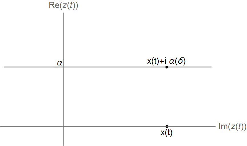
Figure 1: In the restriction $z=x+i\alpha(\delta)$, the imaginary part of $z(t)$ is fixed.

If we consider the restriction $z=x+i\alpha(\delta)$ for (11), which is nothing more than a reparametrization of a line in the complex plane (Fig. 1), the potential becomes

$$V(x+i\alpha) = \cos(2x)\,[\text{cosh}(2\alpha)-\text{sinh}(2\alpha)]$$

$$+i\sin(2x)\,[-\text{sinh}(2\alpha)+\delta\,\text{arccosh}(2\alpha)],$$

where we use basic trigonometric identities. We can take the imaginary part of (LABEL:eq:vxialpha) as null, allowing us to determine $\alpha:\;\left]-1,1\right[\;\to\mathbb{R}$,

$$\alpha(\delta)=\frac{1}{2}\text{arccosh}\left(\sqrt{\frac{1}{1-\delta^{2}}}\right).$$ (13)

Therefore, the map $\mathcal{V}:\mathbb{R}\times\;\left]-1,1\right[\;\to\mathbb{R}$, given by

$$\mathcal{V}(x,\delta)=\sqrt{1-\delta^{2}}\,\sin^{2}(x),$$ (14)

for each $\delta\in\;\left]-1,1\right[\;$, give us a well-defined Hermitian potential. Furthermore, for each fixed $|\delta|<1$, we can rewrite (11) as

$$\left[-\frac{d^{2}}{dx^{2}}-4Q\sin^{2}(x)\right]\psi(x+i\alpha)=(a-2Q)\,\psi(x+i\alpha),$$ (15)

where $Q\equiv q\sqrt{1-\delta^{2}}$ and $\alpha$ is given by (13). These steps allow us to connect both Hermitian and non-Hermitian scenarios. In appendix A, one will note that there is an alternative way to rewrite the generalized $\mathcal{PT}$-symmetric Mathieu potential in a cosineoidal form. It shows that there is no obligation to switch to an axis parallel to the real line. The key point of both methods is the restriction on the values of the $\delta$ deformation parameter. We just have chose to use this first method for convenience.

One may think about another perspective, where the choice is not to nullify the imaginary part of the potential $V(x+i\alpha,\delta)$ in (LABEL:eq:vxialpha), but its real part. In this situation, the equation that establishes the relation between $\alpha$ and $\delta$ parameters is $2\alpha(\delta)=\arctan(i/\delta)$. This corresponds to the complex deformed potential $\mathcal{V}_{Im}(x,\delta)=i\sin(2x)\sqrt{\delta^{2}-1}$ with $|\delta|>1$. It is possible to move the complex number $i$ into the square root, so that it becomes comparable to that with $|\delta|<1$. Briefly,

$$\mathcal{V}(x,\delta) =\cos(2x)\sqrt{1-\delta^{2}},\quad|\delta|<1,$$ (16a)

$$\mathcal{V}_{Im}(x,\delta) =\sin(2x)\sqrt{1-\delta^{2}},\quad|\delta|>1.$$ (16b)

Is is known that the sine and cosine trigonometric functions are equivalent by a ($\pi/2$) phase, then we can write $\sin(2x+\pi/2)=\cos(2x)$. So, if one discovers some applicability of the $\mathcal{V}_{Im}$ imaginary potential, it is possible to summarize both constraints for delta in a single condition, $|\delta|\neq 1$.

IV Resurgent Mathieu partition function with $\delta$-deformation

From (14) we can compute the saddles depending on $\delta$. That is, $S_{p}=\mathcal{V}(0,\delta)=0$ and $S_{np}=\mathcal{V}(\frac{\pi}{2},\delta)=\sqrt{1-\delta^{2}}$. Therefore,

$$Z(\delta,g)=2\int_{0}^{\pi/2}\exp\left(g^{-2}\,\sqrt{1-\delta^{2}}\sin^{2}(x)\right)dx.$$ (17)

Making the change $\sin(x)=s^{2}$ and writing

$$(1-s)^{-1/2}=\sum_{k=0}^{\infty}\frac{\Gamma\left(k+\frac{1}{2}\right)}{\Gamma(k+1)\Gamma\left(\frac{1}{2}\right)},$$ (18)

we have

$$Z(\delta,g^{2})=\frac{1}{g\sqrt{\pi}}\sum_{k=0}^{\infty}\frac{\Gamma(k+\frac{1}{2})}{\Gamma(k+1)\Gamma(\frac{1}{2})}\int_{0}^{1}s^{k-1/2}e^{1/g^{2}\sqrt{1-\delta^{2}}s^{2}}.$$ (19)

Then we apply the Watson’s Lemma to obtain

$$Z(\delta,g^{2})\sim\sum_{k=0}^{\infty}\frac{\left[\Gamma(k+\frac{1}{2})\right]^{2}}{\Gamma(k+1)\Gamma(\frac{1}{2})^{2}}\left(1/g^{2}\sqrt{1-\delta^{2}}\right)^{-k}.$$ (20)

Finally, we have the transseries representation for the $\delta$-deformed Mathieu partition function,

$$Z(\delta,g^{2})= \sigma_{0}\,e^{-S_{p}/g^{2}}\sum_{k=0}^{\infty}a_{0}(k)A^{-k}(\delta,g^{2})$$

$$+\sigma_{1}\,e^{-A(\delta,g^{2})}\sum_{k=0}^{\infty}(-1)^{k}a_{0}(k)A^{-k}(\delta,g^{2}),$$ (21)

where

$$A(\delta,g^{2})=\frac{1}{g^{2}}\sqrt{1-\delta^{2}}.$$ (22)

Furthermore, observe that $\sigma_{0}$ and $\sigma_{1}$ Stokes constants are the same as those appearing in the transseries representation for the usual Hermitian case (6). As expected, this transseries becomes identical to (6) when $\delta$ vanishes. From (22), we can assert that the $g^{2}$ coupling coefficient is subject to a perturbation due to the delta deformation coefficient.

V $\delta$-deformed instanton solution

We now turn to one-dimensional quantum mechanics, in which the partition function is a path integral,

$$\mathcal{Z}(g^{2})=\int\mathcal{D}x\exp\left\{-\int dt\left(\frac{1}{2}m\dot{x}^{2}+\frac{1}{g^{2}}\mathcal{V}(x)\right)\right\}.$$ (23)

Setting $m=1$, the associated instanton equation $\dot{x}(t)=\sqrt{2\mathcal{V}(x(t),\delta)}$ has a solution whose real part is

$$x_{\mathcal{I}}(t)=2\mathrm{arccot}\left(\exp\left(-t\sqrt{2\sqrt{1-\delta^{2}}}\right)\right),$$ (24)

which tends to $\pi$ when $t\rightarrow+\infty$, as shown in Fig. 2(b). The instanton action is also influenced by the $\delta$ parameter,

$$S=\int_{0}^{\pi}\sqrt{2}(1-\delta^{2})^{1/4}\sin(x)dx=2\sqrt{2}\,(1-\delta^{2})^{1/4}.$$ (25)

Since the instanton action is related to singularities in the Borel plane, this amazing result denotes that one could manipulate the position of the singularities in the Borel plane by modifying the value of the non-Hermiticity factor, which characterizes the subject to be explored in a forthcoming paper.

(a) The deformed Mathieu potential in the Hermitian scenario, Eq.(14). As expected, the higher the deformation parameter value, the lower the potential amplitude.

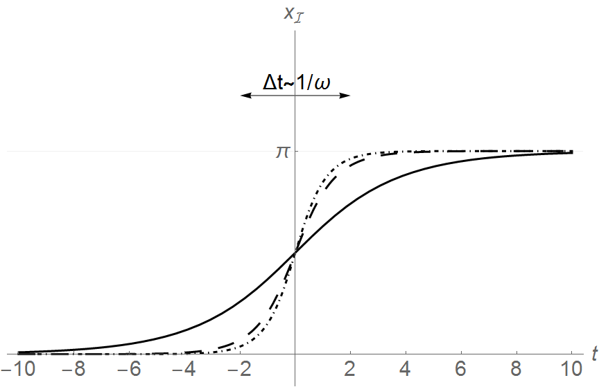
(b) Real instantons in the Hermitian scenario, Eq.(24). We have just observed that the height of the potential barrier decreases as we increase the value of $\delta$ (Fig. 2(a)). This fact does make it smoother for the instanton to pass from one minimum to another. As $\delta\rightarrow 1$, the respective curve resembles a line whose slope is given by $\sqrt{2}(1-\delta^{2})^{1/4}$. The instanton width $\Delta t$ varies with the value of $\delta$, being proportional to $1/\omega=2^{-1/2}(1-\delta)^{-1/4}$

Figure 2: Effects of $\delta$ deformation parameter on (a) $\mathcal{V}(x,\delta)$ potential and (b) $x_{\mathcal{I}}(t)$ instanton solution. The different curves refer to different values of the non-Hermitian parameter: $\delta=0$ (dotted line), $\delta=0.8$ (dashed line) and $\delta=0.996$ (solid line).

Furthermore, in the region permeated by the instanton, there is a guarantee that the $\mathcal{PT}$-symmetry is not broken, because this is a closed scenario and there are still turning points [29].

We’ve already discussed the reason for the restriction $\delta\neq 1$. But what would happen if this was allowed? The potential in (11) with $\delta=1$ is written $V(z,1)=\exp(iz)$. The solution of the instanton equation $\dot{z}=\sqrt{2\,V(z,1)}$ exists, being written as $z_{\mathcal{I}}=2i\ln(-it\sqrt{2}/2)$, although it does not describe a typical instanton curve (Fig. 2(b)). First, we observe that it has a discontinuity in $t=0$. Furthermore, we can assert that the case in which $\delta=1$ does not produce instanton because there are no saddle points.

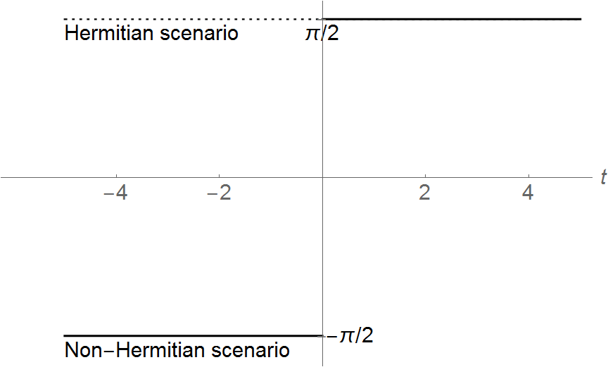
Figure 3: Solid line: Solution of $\dot{z}=\sqrt{2\,V(z,1)}$ for the non-Hermitian scenario of the potential in Eq. (11), with $\delta=1$. Dashed line: Instanton solution for the Hermitian scenario, Eq. (24) with $\delta=1$, which appears as a constant line at $\pi/2$ for all $t$.

We see that the two curves in Fig. 3 do not agree. This is expected, because the non-Hermitian scenario starts with the assumption $\delta=1$. On the other hand, the Hermitian scenario is obtained from the transformation (LABEL:eq:vxialpha) which is valid in the interval $\delta\in\left]-1,1\right[$ (see Eq.(13)). The limit $\delta\rightarrow 1$ is an extrapolation of the latter case and it does not need to be in agreement with the first scenario, as we observe in Fig. 3. It does not bring the complete information. Then, one could naively think that the curves do not need to totally agree with each other, but at least they do in $t>0$.

For the non-Hermitian case, the only analytic solution for the instanton equation is for $\delta=1$, but this is not a true instanton. Recall that, in this scenario, there are no saddle points. Notwithstanding, we have shown that it is possible to investigate the effects of varying the $\delta\in\left]-1,1\right[$ deformation parameter — we finally got true instantons solutions (see Fig. 2(b)). This is done using the connection between non-Hermitian and Hermitian scenarios in section III.

In the following sections, we will see how the behavior of several instantons is affected by the $\delta$ non-Hermiticity factor.

VI Dilute gas of deformed instantons

It is known that instantons are objects that appear in a short time interval [30], having a width on order of $1/\omega$ (see Fig.2(b)). It means that, for large $t=T$, the approximate solutions of the equation of motion are not just instantons and anti-instantons, but also strings of widely separated instantons and anti-instantons. In the case of periodic potentials, in which the Mathieu potential is understood, there are degenerate minima that allow us to sprinkle instantons and anti-instantons freely on the real axis [31, 32]. Thus, we write

$$\braket{j_{+}}{e^{-HT/\hbar}}{j_{-}} = \left(\frac{\omega}{\pi\hbar}\right)^{1/2}\,\exp\left(-\frac{\omega T}{2}\right)$$

$$\times\sum_{n,\bar{n}=0}^{\infty}\frac{(Ke^{-S/\hbar}T)^{n+\bar{n}}}{n!\;\bar{n}!}\delta_{n-\bar{n}+j_{+}+j_{-}},$$

where $n$ is the number of instantons, $\bar{n}$ is the number of anti-instantons. If it were not for the small intervals containing instanton and anti-instanton, $\mathcal{V}^{\prime\prime}(x,\delta)$ would be equal to $\omega^{2}$ on the entire time axis. This characterizes the barrier penetration and that is where the factors before the sum come from. The correction of the formula that includes the influence of multi-instantons is in the summation. The expression $(T^{n+\bar{n}}/(n!\;\bar{n}!))$ is consequence of the integration over the locations of the centers and $K$ is written as

$$K=\left(\frac{S}{2\pi\hbar}\right)^{1/2}\left|\frac{\det(-\partial_{t}^{2}+\omega^{2})}{\det^{\prime}(-\partial_{t}^{2}+\mathcal{V}^{\prime\prime}(\bar{x}))}\right|^{1/2},$$ (27)

where $\bar{x}$ is a single instanton and $\det^{\prime}$ means that the zero eigenvalue is omitted when computing the determinant.

The terms of an exponential series $\sum_{k=0}^{\infty}y^{k}/k!$ grow with $k$, for any fixed $y$, just until $k$ is on the order of $y$. Then, they begin to decrease fast. We can apply this to the sum in Eq. (27) to conclude that the important terms are those for which the number of (anti-)instantons is less or approximately $(Ke^{-S/\hbar}\,T)$. For small $\hbar$, it means that the density of (anti-)instantons is exponentially small when considering this important terms. Thus, the average separation is huge. This is why this approach is called the dilute gas approximation of instantons. The conditions of the validity of average separation do not depend on $T$, as long as $T$ is sufficiently large.

From the instanton solution, Eq. (24), we identify $\omega$, see Fig. 2(b). The expression that describes the instanton action is in Eq. (25). By comparison, we have $S=2\omega=2\sqrt{2}(1-\delta)^{1/4}$. Then, we can already note that the deformation parameter is strongly present even at the multi-instantons level.

The following section goes beyond the dilute instanton gas approximation and shows a case where there is an interaction between coupled instanton–anti-instanton.

VII Josephson junctions described by tilted $\delta$-deformed washboard potential

The Josephson effect is a phenomenon that occurs when two or more superconductors are placed next to each other, with some potential barrier or restriction between them. This arrangement generates a supercurrent that flows through this device known as the Josephson junction. There are ways to build superconducting circuits based on the Josephson junction. They are candidates for developing quantum computing devices. As an example of this type, we have the superconducting quantum interference device (SQUID) [33].

In this context, the role of tunneling coordinate across the Josephson junction is played by the phase difference of the Cooper pair wave function. The standard model for describing this coupling is the resistively shunted junction (RSJ) model,

$$C\left(\frac{\phi_{0}}{2\pi}\right)^{2}\frac{d^{2}\psi}{dt^{2}}+\frac{1}{R}\left(\frac{\phi_{0}}{2\pi}\right)^{2}\frac{d\psi}{dt}+E_{J}\sin\psi-I_{\textrm{ext}}\frac{\phi_{0}}{2\pi}=0,$$ (28)

where $C$ and $R$ are respectively the capacitance and the effective shunt resistance of the junction, $\phi_{0}=h/2e$ is the flux quantum, $I_{\textrm{ext}}$ is the external bias current, and $E_{J}=I_{c}\phi_{0}/2\pi$ is the Josephson coupling energy, which is related with the $I_{c}$ maximum supercurrent suported by the junction.

There is a parallel between the equation of motion of this model, Eq. (28), and the one corresponding to the motion of a Brownian particle of mass $M$ and position $X$ in the absence of fluctuations [33], given by

$$M\ddot{X}+M\gamma X(t)+\frac{\partial V(X)}{\partial X}=0,$$ (29)

where the potential is known as the tilted washboard, which is nothing more than trigonometric shape potential with a tilt. Note that we can insert the potential (14) of the Hermitian scenario in this context if we include a term for the tilt and make $x=\pi X/X_{0}$. Thus, we write

$$V(X)=-\frac{\sqrt{1-\delta^{2}}}{2}V_{0}\left[\cos\left(\frac{2\pi X}{X_{0}}\right)-\frac{1}{2}\right]-V_{\textrm{tilt}}\left(\frac{2\pi X}{X_{0}}\right),$$ (30)

where and $\delta\in\left]-1,1\right[$. Comparing the equations (28), (29) and (30), we see that there is a equivalence relation $(V_{0}/2)\sqrt{1-\delta^{2}}\;\hat{=}\;E_{J}$. A simple algebraic manipulation generates

$$|\delta|\;\hat{=}\;\sqrt{1-\frac{I^{2}_{c}h^{2}}{4V_{0}^{2}\pi^{2}e^{2}}}.$$ (31)

Therefore, the insertion of the tilted deformed Mathieu potential (30) in the Brownian motion equation (29) allows relating the non-Hermiticity factor $\delta$ with the $I_{c}$ Josephson supercurrent.

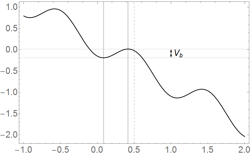
(a) The tilted $\delta$-deformed washboard potential (30) with $\delta=0.8$, $X_{0}=1$, $V_{\textrm{tilt}}=0.15J$, $V_{0}=1.0J$. This exemplifies the case $|\delta|<\sqrt{1-4V_{\textrm{tilt}}^{2}/V_{0}^{2}}$. The critical points in the interval $0<X<X_{0}/2$ are the minimum $X_{1}=(X_{0}/2\pi)\arcsin\left(V_{\textrm{tilt}}/(V_{0}\sqrt{1-\delta^{2}}/2)\right)$ and the maximum $X_{2}=(X_{0}/2)-X_{1}$. The height of the barrier is $V_{b}=V(X_{2})-V(X_{1})$, explicitly written in the Eq. (32). Thick gridlines: minimum and maximum positions. Dashed gridline: $X_{0}/2$.

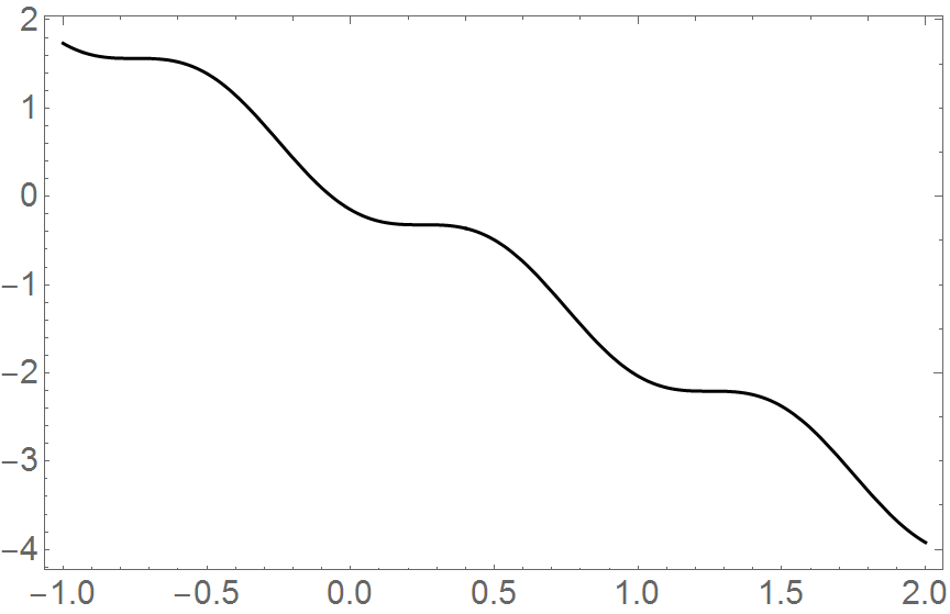
(b) An example of the case $|\delta|=\sqrt{1-4V_{\textrm{tilt}}^{2}/V_{0}^{2}}$, where we choose $\delta=0.8$, $V_{\textrm{tilt}}=0.3J$, $V_{0}=1.0J$, $X_{0}=1$. There are no cascade barriers.

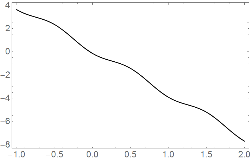
(c) An example of the case $|\delta|>\sqrt{1-4V_{\textrm{tilt}}^{2}/V_{0}^{2}}$, where we choose $\delta=0.8$, $V_{\textrm{tilt}}=0.6J$, $V_{0}=1.0J$, $X_{0}=1$. The slope of the potential is negative for all $X$.

Figure 4: The tilted $\delta$-deformed washboard potential (30) for (a) $|\delta|<\sqrt{1-4V_{\textrm{tilt}}^{2}/V_{0}^{2}}$, (b) $|\delta|=\sqrt{1-4V_{\textrm{tilt}}^{2}/V_{0}^{2}}$ and (c) $|\delta|>\sqrt{1-4V_{\textrm{tilt}}^{2}/V_{0}^{2}}$.

There are two distinct states in this current-biased Josephson junction: the zero-voltage state, which corresponds to the particle being trapped in a well, and the voltage state, that represents the particle sliding down the cascade of wells. Figure 4(a) makes it easy to see that the height of the barrier $V_{b}$ can be calculated by the difference between the value of the potential (30) at a maximum and its value at the previous minimum, such that

$$V_{b}=2\sqrt{\left(\frac{1-\delta^{2}}{4}\right)V_{0}^{2}-V_{\textrm{tilt}}^{2}}-2V_{\textrm{tilt}}\arccos\left(\frac{V_{\textrm{tilt}}/V_{0}}{\sqrt{1-\delta^{2}}/2}\right).$$ (32)

From this result, we can see three different events. There are no cascade barriers for $|\delta|=\sqrt{1-4V^{2}_{\textrm{tilt}}/V_{0}^{2}}$. The particle slides all the way down for $|\delta|>\sqrt{1-4V^{2}_{\textrm{tilt}}/V_{0}^{2}}$. Finally, the proper condition for tunneling is $|\delta|<\sqrt{1-4V^{2}_{\textrm{tilt}}/V_{0}^{2}}$. An interesting case within this last regime occurs when $|\delta|\ll\sqrt{1-4V^{2}_{\textrm{tilt}}/V_{0}^{2}}$. In this limit, the bounce is described by a weakly bound instanton–anti-instanton pair. The distance between them is large compared to the width of an instanton. Thus, the action of the bounce is written

$$S(T)/\hbar=2S_{\mathcal{I}}/\hbar+W(T)-\epsilon T,$$ (33)

where the action of a single instanton is

$$S_{\mathcal{I}}=\frac{M\gamma X_{0}^{2}}{2\pi\hbar}\left[1+\ln\left(\pi^{2}V_{0}\sqrt{1-\delta^{2}}/(M\gamma X_{0}^{2}\omega_{c})\right)\right],$$ (34)

the interaction term between the instantons at a distance $T$ is

$$W(T)=\frac{M\gamma X_{0}^{2}}{\pi\hbar}\ln[(\hbar\beta\omega_{c}/\pi)\sin(\pi T/\hbar\beta)],$$ (35)

with $\omega_{c}$ taking the role of a reference frequency, and the last term $\epsilon T$ comes from the potential drop $\hbar\epsilon=2\pi V_{\textrm{tilt}}$ on the distance $X_{0}$.

VIII Conclusion

In this work, we studied the implications of a $\mathcal{PT}$-symmetry deformation parameter $\delta$ in the transseries representation of the Mathieu partition function and in the instanton solution of the $\delta$-dependent Mathieu potential. First, we sought to establish a connection between the Hermitian and non-Hermitian scenarios. In order to do this, we worked with a non-Hermiticity factor restricted to the interval $\left]-1,1\right[$. We found that the deformation parameter is explicitly present in the non-perturbative saddle action and in the two formal series, perturbing the coupling coefficient. Therefore, the value of $\delta$ affects the transseries representation. Furthermore, we showed that the width of the real instanton solution increases as the value of $\delta$ grows (tending to 1). Such a fact makes it smoother for the instanton to pass from one minimum to another. Our third observation was that the deformation parameter is present even at the multi-instanton scenario, characterizing a dilute gas of deformed instantons. We also studied the interesting case in which we make a parallel with the Josephson junction through a tilted deformed washboard potential. In the regime in which the bounce corresponds to a widely spaced instanton-anti-instanton pair, the $\mathcal{PT}$-deformation factor is present in the action of the bounce and affects the height of the potential barrier. We found that we can relate the non-Hermiticity factor with the Josephson supercurrent, indicating that the deformation might have a physical meaning.

Appendix A Working at the original axis

In Sec. III, we have used the reparameterization $z=x+i\alpha(\delta)$ on the generalized $\mathcal{PT}$-symmetric Mathieu equation (11). It has allowed us to connect Hermitian and non-Hermitian scenarios and to perform calculations in the referential given by this line parallel to the real axis, in the complex plane (see Fig.1). We choose this method by convenience, but this is not the only way to rewrite the $\mathcal{PT}$-symmetric Mathieu potential. We show in this appendix that we can keep the complex variable $z$ unchanged in this process.

Consider multiplying the potential in Eq.(11) by a factor $\cos(i\epsilon)$,

$$\cos(i\epsilon)V(z,\delta)=\cos(i\epsilon)\cos(2z)+i\delta\cos(i\epsilon)\sin(2z).$$ (36)

If we define $\delta$ such that $\delta\cos(i\epsilon)=-\sinh(\epsilon)$, or equivalently,

$$\delta=-\tanh(\epsilon).$$ (37)

This causes the same restriction on $\delta$ values that we have found in the section III, that is, $\delta\in\;\left]-1,1\right[\;$. We can write the deformed potential as

$$\mathcal{V}(z,\delta)=\frac{\cos(2z+i\epsilon)}{\cos(i\epsilon)}.$$ (38)

Thus, we can conclude that it is enough to restrict the values of the non-Hermiticity factor to the interval $\delta\in\;\left]-1,1\right[\;$ in order to achieve the trigonometric form of the potential (Eq. 38). To conveniently calculate the instanton solution of this potential, $\dot{z}(t)=\sqrt{2\mathcal{V}(z(t),\delta)}$, we can rewrite it as

$$\mathcal{V}(z,\delta)=\frac{2\sin^{2}(z+i\epsilon)}{\cos(i\epsilon)}.$$ (39)

Thus, we find

$$z_{\mathcal{I}}(t)=-i\epsilon+2\left\{\mathrm{arctan}\left[\exp\left(2t\sqrt{\mathrm{sech}(\epsilon)}\right)\right]\right\}.$$ (40)

We can find the $\epsilon$ values corresponding to the $\delta$ values used in Fig. 2(b) through Eq. 37. The $\mathrm{Re}\,z_{\mathcal{I}}(t)$ curves in Fig. 5 are identical to the $x_{\mathcal{I}}(t)$ curves plotted in Fig. 2(b)).

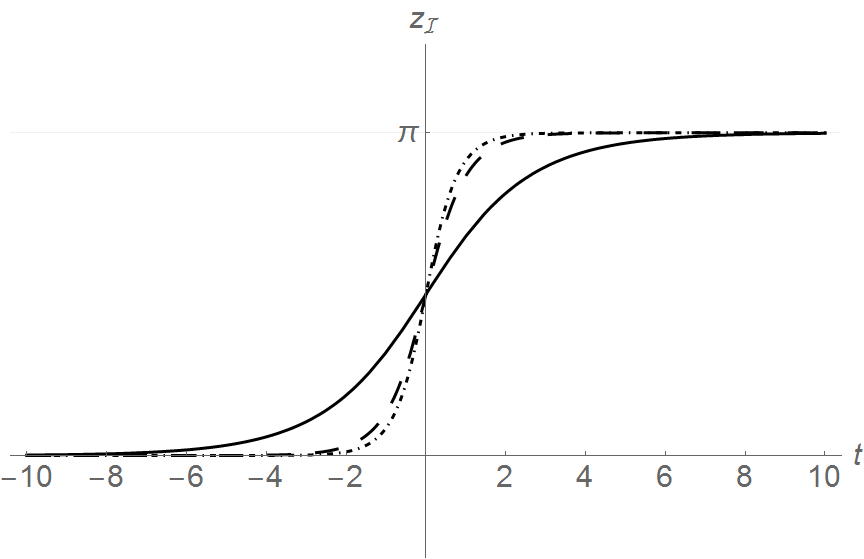
Figure 5: Real part of instanton solution $z_{\mathcal{I}}(t)$ (40) for $\epsilon=0$ (dotted line), $\epsilon=1.099$ (dashed line) and $\epsilon=3.106$ (solid line).

References

- Mathieu [1868] É. Mathieu, Mémoire sur le mouvement vibratoire d’une membrane de forme elliptique, J. Math. Pures Appl. 13, 137 (1868).
- McLachlan [1947] N. W. McLachlan, Theory and Application of Mathieu Functions (Clarendon Press, London, 1947).
- Coïsson et al. [2009] R. Coïsson, G. Vernizzi, and X. Yang, Mathieu functions and numerical solutions of the Mathieu equation, in 2009 IEEE International Workshop on Open-source Software for Scientific Computation (OSSC) (2009) pp. 3–10.
- Li and Wang [2000] S. Li and B. S. Wang, Field expressions and patterns in elliptical waveguide, IEEE Transactions on Microwave Theory and Techniques 48, 864 (2000).
- Stanley Humphries [1956] J. Stanley Humphries, Principles of Charged Particle Acceleration (Wiley, New York, 1956).
- Winter and Ortjohann [1991] H. Winter and H. W. Ortjohann, Simple demonstration of storing macroscopic particles in a “Paul trap”, Am. J. Phys. 59, 807 (1991).
- Carver [1971] T. R. Carver, Mathieu’s functions and electrons in a periodic lattice, Am. J. Phys. 39, 1225 (1971).
- Aldrovandi and Ferreira [1980] R. Aldrovandi and P. L. Ferreira, Quantum pendulum, Am. J. Phys. 48, 660 (1980).
- Kerner et al. [2012] R. Kerner, G. Naumis, and W. A. Gómez-Arias, Bending and flexural phonon scattering: Generalized Dirac equation for an electron moving in curved graphene, Physica B: Condensed Matter 407, 2002 (2012).
- Cherman et al. [2015a] A. Cherman, D. Dorigoni, and M. Ünsal, Decoding perturbation theory using resurgence: Stokes phenomena, new saddle points and Lefschetz thimbles, JHEP 10, 056, arXiv:1403.1277 [hep-th] .
- Cherman et al. [2015b] A. Cherman, P. Koroteev, and M. Ünsal, Resurgence and holomorphy: from weak to strong coupling, J. Math. Phys. 56, 053505 (2015b), arXiv:1410.0388 [hep-th] .
- Başar et al. [2013] G. Başar, G. Dunne, and M. Ünsal, Resurgence theory, ghost-instantons, and analytic continuation of path integrals, JHEP 10, 041, arXiv:1308.1108 [hep-th] .
- Wigner [1932] E. Wigner, The operation of time reversal in quantum mechanics, Nachr. Ges. Wiss. Göttingen Math.-Physik. Kl. 1, 546 (1932).
- Makris et al. [2008] K. G. Makris, R. El-Ganainy, D. N. Christodoulides, and Z. H. Musslimani, Beam dynamics in symmetric optical lattices, Phys. Rev. Lett. 100, 103904 (2008).
- Bender and Boettcher [1998] C. M. Bender and S. Boettcher, Real spectra in non-hermitian hamiltonians having symmetry, Phys. Rev. Lett. 80, 5243 (1998).
- Bender [2016] C. M. Bender, symmetry in quantum physics: From a mathematical curiosity to optical experiments, Europhysics News 47, 17 (2016).
- Bender [2018] C. M. Bender, Symmetry in Quantum and Classical Physics (World Scientific, Singapore, 2018).
- Cavalcanti et al. [2022] E. Cavalcanti, N. M. Alvarenga, F. Reis, J. R. Mahon, C. A. Linhares, and J. A. Lourenço, Energy levels for -symmetric deformation of the Mathieu equation, (2022), arXiv:2204.13350 [quant-ph] .
- Zinn-Justin and Jentschura [2004] J. Zinn-Justin and U. D. Jentschura, Multi-instantons and exact results I: conjectures, WKB expansions, and instanton interactions, Annals of Physics 313, 197 (2004).
- Mariño [2015] M. Mariño, Instantons and Large N: An Introduction to Non-Perturbative Methods in Quantum Field Theory (Cambridge University Press, 2015).
- Mariño [2014] M. Mariño, Lectures on non-perturbative effects in large n gauge theories, matrix models and strings, Fortschr. Phys. 62, 455 (2014).
- Aniceto et al. [2019] I. Aniceto, G. Başar, and R. Schiappa, A primer on resurgent transseries and their asymptotics, Phys. Rep. 809, 1 (2019).
- Aniceto and Schiappa [2015] I. Aniceto and R. Schiappa, Nonperturbative ambiguities and the reality of resurgent transseries, Commun. Math. Phys. 335, 183 (2015).
- [24] DLMF, NIST Digital Library of Mathematical Functions, http://dlmf.nist.gov/28, Release 1.1.6 of 2022-06-30, f. W. J. Olver, A. B. Olde Daalhuis, D. W. Lozier, B. I. Schneider, R. F. Boisvert, C. W. Clark, B. R. Miller, B. V. Saunders, H. S. Cohl, and M. A. McClain, eds.
- Alvarenga [2020] N. M. Alvarenga, Resurgence Theory Applied to Quantum Mechanics, Ph.D. thesis, Universidade do Estado do Rio de Janeiro (2020), in Portuguese.
- Tanizaki [2015] Y. Tanizaki, Study on Sign Problem via Lefschetz-Thimble Path Integral, Ph.D. thesis, University of Tokyo (2015).
- Serone et al. [2017] M. Serone, G. Spada, and G. Villadoro, The power of perturbation theory, JHEP 56, 1029, arXiv:1702.04148 [hep-th] .
- Bender and Orszag [1999] C. M. Bender and S. A. Orszag, Advanced Mathematical Methods for Scientists and Engineers I: Asymptotic Methods and Perturbation Theory (Springer, 1999).
- Bender and Hook [2021] C. M. Bender and D. W. Hook, -symmetric classical mechanics, (2021), arXiv:2103.04214 [math-ph] .
- Das [2006] A. Das, Field Theory: A Path Integral Approach, 2nd ed. (World Scientific, Singapore, 2006) https://www.worldscientific.com/doi/pdf/10.1142/6145 .
- Coleman [1985] S. Coleman, Aspects of Symmetry (Cambridge University Press, 1985).
- Zinn-Justin [1982] J. Zinn-Justin, The principles of instanton calculus: a few applications, in Les Houches Summer School on Theoretical Physics: New Trends in Atomic Physics (1982).
- Weiss [2008] U. Weiss, Quantum Dissipative Systems, 3rd ed. (World Scientific, 2008).