Tensor Decompositions for Count Data that Leverage Stochastic and Deterministic Optimization

Abstract

There is growing interest to extend low-rank matrix decompositions to multi-way arrays, or tensors. One fundamental low-rank tensor decomposition is the canonical polyadic decomposition (CPD). The challenge of fitting a low-rank, nonnegative CPD model to Poisson-distributed count data is of particular interest. Several popular algorithms use local search methods to approximate the global maximum likelihood estimator from local minima. Simultaneously, a recent trend in theoretical computer science and numerical linear algebra leverages randomization to solve very large, hard problems. The typical approach is to use randomization for a fast approximation and determinism for refinement to yield effective algorithms with theoretical guarantees. Two popular algorithms for Poisson CPD reflect that emergent dichotomy: CP Alternating Poisson Regression is a deterministic algorithm and Generalized Canonical Polyadic decomposition makes use of stochastic algorithms in several variants. This work extends recent work to develop two new methods that leverage randomized and deterministic algorithms for improved accuracy and performance.

15A69, 65F55

1 Introduction

Low-rank tensor decompositions in general, and the canonical polyadic decomposition (CPD) specifically, are becoming increasingly important for multi-way data analysis. The challenge of fitting a low-rank, nonnegative CPD model to count data is often formulated as a nonlinear, nonconvex global optimization problem. When the data is assumed to be Poisson-distributed, one approach is to determine the optimal Poisson parameters that maximize the likelihood of the data via tensor maximum likelihood estimation. The global optimizer to the optimization problem is the maximum likelihood estimator (MLE). Since global optimization algorithms are often prohibitively expensive for tensor data, great emphasis has been placed on developing efficient local methods for finding the Poisson CPD parameters. In practice, local methods for solving global optimization problems are often orchestrated in a multi-start strategy–—i.e., computing a set of approximations from many random starting points—–to increase the probability that the model best approximating the MLE has been found. However, this approach demands significant computational resources when high-confidence solutions are required and may lead to excessive computations even for small problems. To mitigate this issue, we examine the role of randomization and determinism in Poisson CPD solvers.

Our contributions are:

• two Poisson CPD methods that compute the MLE with higher probability than current effective local search methods, and

• validation of our methods with open-source software on synthetic data.

Our first method is HybridGC, which uses a two-stage hybrid strategy built from effective local methods. Generalized CP decomposition (GCP) [37, 47] incorporates general loss functions, including Poisson loss, and stochastic optimization methods. The first stage of HybridGC uses GCP with stochastic optimization to form a quick approximation and helps the method avoid local minima that are not the MLE. CP Alternating Poisson Regression (CPAPR) [18] is a deterministic Poisson CPD method that alternates over a sequence of convex Poisson loss subproblems iteratively. Previously, in [56], we showed that CPAPR is performant and can compute accurate approximations to the MLE with higher probability than GCP. The second stage uses CPAPR to refine the approximation from GCP to higher accuracy.

Our second method is Restarted CPAPR with SVDrop, which is a variant of an effective local method that computes a heuristic called SVDrop to detect convergence to a rank-deficient solution. Rank-deficiency violates the assumptions of the Poisson CPD model and is therefore unacceptable. Our experiments demonstrate empirically that there is a strong connection between rank-deficiency and local minimizers that are not the MLE. When SVDrop identifies such a solution, the local method is restarted from a random point in the feasible domain.

In Section 2, we introduce notation, provide the necessary background, and discuss related work. In Section 3, we formalize several metrics to compare CPD methods, some of which we used previously in [56]. In Section 4, we describe the data used in numerical experiments. In Section 5, we introduce Hybrid GCP-CPAPR (HybridGC). In Section 6, we introduce Restarted CPAPR with SVDrop. In our experiments, we demonstrate that both methods often improve the likelihood of convergence to the MLE, thereby reducing excessive computations when compared to multi-start where the local methods are standalone solvers. In Section 7, we propose future work.

2 Background and related work

2.1 Notation and conventions

The set of real numbers and integers are denoted as $\mathbb{R}$ and $\mathbb{Z}$, respectively. The real numbers and integers restricted to nonnegative values are denoted as $\mathbb{R}_{+}$ and $\mathbb{Z}_{+}$, respectively. The order of a tensor is the number of dimensions or ways. Each tensor dimension is called a mode. A scalar (tensor of order zero) is represented by a lowercase letter, e.g., $x$. A bold lowercase letter denotes a vector (tensor of order one), e.g., $\bm{\mathbf{v}}$. A matrix (tensor of order two) is denoted by a bold capital letter, e.g., $\bm{\mathbf{A}}\in\mathbb{R}^{m\times n}$. Tensors of order three and higher are expressed with a bold capital script letter, e.g., $\bm{\mathscr{X}}\in\mathbb{R}^{m\times n\times p}$. Values computed, approximated, or estimated are typically written with a hat—e.g., $\bm{\mathscr{\widehat{M}}}\in\mathbb{R}^{m\times n\times p}$ may be a tensor model of parameters approximating the data tensor $\bm{\mathscr{X}}$.

The $i$-th entry of a vector $\bm{\mathbf{v}}$ is denoted $v_{i}$, the $(i,j)$ entry of a matrix $\bm{\mathbf{M}}$ is denoted $m_{ij}$, and the $(i,j,k)$ entry of a three-way tensor $\bm{\mathscr{X}}$ is denoted $x_{ijk}$. Fibers are the higher-order analogue of matrix rows and columns. Indices are integer values that range from 1 to a value denoted by the capitalized version of the index variable, e.g., $i=1,\ldots,I$. We use MATLAB-style notation for subarrays formed from a subset of indices of a vector, matrix, or tensor mode. We use the shorthand $i_{j}\colon i_{k}$ when the subset of indices forming a subarray is the range $i_{j},\ldots,i_{k}$. The special case of a colon $\colon$ by itself indicates all elements of a mode, e.g., the $j$-th column or mode-1 fiber of the matrix $\bm{\mathbf{A}}$ is $\bm{\mathbf{A}}(\colon,j)=\bm{\mathbf{A}}(i_{1}\colon i_{I},j)$. We use the multi-index

(1) $$\bm{\mathbf{i}}\coloneqq(i_{1},i_{2},\ldots,i_{d})\quad\text{with}\quad i_{j}\in\{1,2,\ldots,I_{j}\}\quad\text{for}\quad j=1,\ldots,d,$$

as a convenient shorthand for the $(i_{1},i_{2},\ldots,i_{d})$ entry of a $d$-way tensor.

Superscript $T$ denotes non-conjugate matrix transpose. We assume vectors $\bm{\mathbf{u}}$ and $\bm{\mathbf{v}}$ are column vectors so that $\bm{\mathbf{u}}^{T}\bm{\mathbf{v}}$ is an inner product of vectors and $\bm{\mathbf{u}}\bm{\mathbf{v}}^{T}$ is an outer product of vectors. We also denote outer products of vectors as $\bm{\mathbf{u}}\circ\bm{\mathbf{v}}=\bm{\mathbf{u}}\bm{\mathbf{v}}^{T}$, which is especially useful when describing the $d$-way outer products of $d$ vectors for $d\geq 2$. The number of matrix or tensor non-zero elements is denoted $\operatorname{nnz}(\cdot)$; conversely, the number of zeros in a matrix or tensor is denoted $\operatorname{nz}(\cdot)$.

2.2 Matricization: transforming a tensor into a matrix

Matricization, as defined in [46], also known as unfolding or flattening, is the process of reordering the elements of a $d$-way array into a matrix. The mode-$n$ matricization of a tensor $\bm{\mathscr{X}}\in\mathbb{R}^{I_{1}\times I_{2}\times\dots\times I_{d}}$, denoted $\bm{\mathbf{X}}_{(n)}$, arranges the mode-$n$ fibers to be the columns of the resulting matrix.

2.3 Canonical polyadic decomposition

The canonical polyadic decomposition (CPD) represents a tensor as a finite sum of rank-one outer products, a generalization of the matrix singular value decomposition (SVD) to tensors. One major distinction is that there are no orthogonality constraints on the vectors of the CPD model. Thus we treat the matrix SVD as a special case of the CPD. Nonetheless, low-rank CP decompositions are appealing for reasons similar to those of the low-rank SVD, including dimensionality reduction, compression, de-noising, and more. Interpretability of CP decompositions on real problems is well-documented, with applications including exploratory temporal data analysis and link prediction [20], chemometrics [55], neuroscience [4], and social network and web link analysis [45, 46].

One particular application of interest is when the tensor data are counts. In this case, a common modeling choice is to assume that the data follow a Poisson distribution so that statistical methods, like maximum likelihood estimation, can be applied to the analysis. One key challenge for computing the Poisson CPD is that a low-rank CP tensor model of Poisson parameters must satisfy certain nonnegativity and stochasticity constraints. In the next few sections we cover the details of the low-rank CP tensor models of Poisson parameters and decompositions which are the focus of this work.

2.4 Low-rank CP tensor model

Assume $\bm{\mathscr{X}}$ is a $d$-way tensor of size $I_{1}\times\dots\times I_{d}$. The tensor $\bm{\mathscr{X}}$ is rank-one if it can be expressed as the outer product of $d$ vectors, each corresponding to a mode in $\bm{\mathscr{X}}$, i.e.,

(2) $$\bm{\mathscr{X}}=\bm{\mathbf{a}}_{1}\circ\bm{\mathbf{a}}_{2}\circ\dots\circ\bm{\mathbf{a}}_{d}.$$

More broadly, the rank of a tensor $\bm{\mathscr{X}}$ is the smallest number of rank-one tensors that generate $\bm{\mathscr{X}}$ as their sum [46]. We concentrate on the problem of approximating a tensor of data with a low-rank CP tensor model, i.e., the sum of relatively few rank-one tensors.

Let $\bm{\lambda}=[\lambda_{1},\lambda_{2},\ldots,\lambda_{d}]\in\mathbb{R}^{d}$ be a vector of scalars and let $\bm{\mathbf{A}}_{1}\in\mathbb{R}^{I_{1}\times R}$, $\bm{\mathbf{A}}_{2}\in\mathbb{R}^{I_{2}\times R}$, $\ldots,$ $\bm{\mathbf{A}}_{d}\in\mathbb{R}^{I_{d}\times R}$ be matrices. The rank-$R$ canonical polyadic (CP) tensor model of $\bm{\mathscr{X}}$ [30, 16] is:

(3) $$\bm{\mathscr{X}}\approx\bm{\mathscr{M}}=\llbracket\bm{\lambda};\bm{\mathbf{A}}_{1},\ldots,\bm{\mathbf{A}}_{d}\rrbracket\coloneqq\sum_{r=1}^{R}\lambda_{r}\bm{\mathbf{A}}_{1}(\colon,r)\circ\dots\circ\bm{\mathbf{A}}_{d}(\colon,r).$$

Each $\bm{\mathbf{A}}_{k}\in\mathbb{R}^{I_{k}\times R}$ is a factor matrix with $I_{k}$ rows and $R$ columns. The $j$-th component of the mode-$k$ factor matrix is the column vector $\bm{\mathbf{A}}_{k}(\colon,j)$. We refer to the form $\bm{\mathscr{M}}=\llbracket\bm{\lambda};\,\bm{\mathbf{A}}_{1},\ldots,\bm{\mathbf{A}}_{d}\rrbracket$ as a Kruskal tensor.

2.5 Computing the Poisson CPD for count data

We focus on an application where all of the entries in a data tensor are counts. For the remainder of this work, let $\bm{\mathscr{X}}\in\mathbb{Z}_{+}^{I_{1}\times\dots\times I_{d}}$ be a $d$-way tensor of nonnegative integers, let $\bm{\mathscr{M}}$ be a CP tensor model of the form Eq. 3, and assume the following about $\bm{\mathscr{X}}$:

1. each $x_{\bm{\mathbf{i}}}\in\bm{\mathscr{X}}$ is sampled from a Poisson distribution with parameter $m_{\bm{\mathbf{i}}}$,

2. the tensor $\bm{\mathscr{X}}$ has low-rank structure,

3. the relationships between the entries in $\bm{\mathscr{X}}$ can be modeled well using a multilinear form, and

4. the rank of $\bm{\mathscr{X}}$ is known a priori.

Chi and Kolda showed in [18] that under these assumptions a Poisson CP tensor model is an effective low-rank approximation of $\bm{\mathscr{X}}$. The Poisson CP tensor model has shown to be valuable in analyzing latent patterns and relationships in count data across many application areas, including food production [15], network analysis [21, 12], term-document analysis [17, 34], email analysis [14], link prediction [20], geospatial analysis [23, 33], web page analysis [44], and phenotyping from electronic health records [35, 36, 32]

One numerical approach to fit a low-rank Poisson CP tensor model to data is tensor maximum likelihood estimation, which has proven to be successful. Computing the Poisson CPD via tensor maximum likelihood estimation involves minimizing the following nonlinear, nonconvex optimization problem:

(4) $$\min_{\bm{\mathscr{M}}}f\left(\bm{\mathscr{X}},\bm{\mathscr{M}}\right)=\min\sum_{\bm{\mathbf{i}}}m_{\bm{\mathbf{i}}}-x_{\bm{\mathbf{i}}}\log m_{\bm{\mathbf{i}}},$$

where $\bm{\mathbf{i}}$ is the multi-index Eq. 1, $x_{\bm{\mathbf{i}}}\geq 0$ is an entry in $\bm{\mathscr{X}}$, and $m_{\bm{\mathbf{i}}}>0$ is a parameter in the Poisson CP tensor model $\bm{\mathscr{M}}$. The function $f(\bm{\mathscr{X}},\bm{\mathscr{M}})$ in Eq. 4 is the negative of the log-likelihood of the Poisson distribution (omitting the constant $\sum_{\bm{\mathbf{i}}}\log\left(x_{\bm{\mathbf{i}}}!\right)$ term) [63]. We will refer to it simply as Poisson loss.

In contrast to linear maximum likelihood estimation [58], where a single parameter is estimated using multiple data instances, tensor maximum likelihood estimation fits a single parameter in an approximate low-rank model to a single data instance. Within the tensor context, low-rank structure means that multiple instances in the data are linked to a single model parameter, a type of multilinear maximum likelihood estimation. This distinction is not made anywhere else in the literature, to the best of our knowledge.

Much of the research associated with computing the low-rank Poisson CPD via tensor maximum likelihood estimation has focused on local methods [18, 29, 37, 47], particularly with respect to computational performance [65, 57, 60, 8, 51, 9, 11]. Many of the current local methods for Poisson CPD can be classified as either an alternating [16, 30] or an all-at-once [1, 2, 59] optimization method.

Alternating local methods iteratively solve a series of subproblems by fitting each factor matrix sequentially while the remaining factor matrices are held fixed. These methods are a form of coordinate descent (CD) [68], where each factor matrix is a block of components that is fit while the remaining component blocks (i.e., factor matrices) are left unchanged. Since each block corresponds to a lower-dimensional problem, alternating tensor methods employ block CD iteratively to solve a series of easier problems. CP Alternating Poisson Regression (CPAPR) was introduced by Chi and Kolda in [18] as a nonlinear Gauss-Seidel approach to block CD that uses a fixed-point majorization-minimization algorithm called Multiplicative Updates (CPAPR-MU). At the highest level, the CPAPR algorithm performs an outer iteration where optimizations are applied on each mode in an alternating fashion. An inner iteration is an optimization using multiplicative updates applied to a subset of variables corresponding to an individual mode. Inner iterations are performed until the convergence criterion is satisfied for a mode or up to the maximum allowable number, $l_{max}$. Outer iterations are performed until the convergence criterion is satisfied for the whole model or up to the maximum allowable number, $k_{max}$. The convergence criterion is based on the Karush-Kuhn-Tucker (KKT) conditions, necessary conditions for convergence to a local minimum in nonlinear optimization. A local minimizer that satisfies the KKT conditions is called a KKT point.

Hansen et al. in [29] presented two Newton-based, active set gradient projection methods using up to second-order information, Projected Damped Newton (CPAPR-PDN) and Projected Quasi-Newton (CPAPR-PQN). Moreover, they provided extensions to these methods where each component block of the CPAPR minimization can be further separated into independent, highly-parallelizable row-wise subproblems; these methods are Projected Damped Newton for the Row subproblem (CPAPR-PDNR) and Projected Quasi-Newton for the Row subproblem (CPAPR-PQNR).

One outer iteration of all-at-once optimization methods updates all optimization variables simultaneously. The Generalized Canonical Polyadic decomposition algorithm (GCP) [37] is a gradient descent method based on a generic formulation of first derivative information for arbitrary loss functions to compute the CPD via tensor maximum likelihood estimation. The original GCP method has two variants: 1) deterministic, which uses limited-memory quasi-Newton optimization (L-BFGS) and 2) stochastic, which supports gradient descent (SGD), AdaGrad [19], and Adam [42] optimizations. The stochastic variants perform loss function and gradient computations on samples of the input data tensor so that the search path is computed from estimates of these values. We focus here on GCP-Adam [47], which applies Adam for scalability.

More generally, we focus on the GCP and CPAPR families of tensor maximum likelihood-based local methods for Poisson CPD for the following reasons:

1. Existing Theory: Method convergence, computational costs, and memory demands are well-understood.

2. Available Software: High-level MATLAB implementing both families is available in MATLAB Tensor Toolbox (TTB) [7, 6]. A Python version is available in pyttb. High performance C++ code that leverages the Kokkos hardware abstraction library [22] to provide parallel computation on diverse computer architectures (e.g., x86-multicore, GPU, etc.) is available with SparTen for CPAPR [65] and Genten for GCP [60]. Additional open-source software for MATLAB includes N-Way Toolbox [3] and Tensorlab [67]. Commercial software includes ENSIGN Tensor Toolbox [10].

2.6 Related work

There are other approaches in the literature that seek to fit models with other distributions in the exponential family or that use other algorithms to estimate parameters. Alternating least squares methods are relatively easy to implement and effective when used with LASSO-type regularization [24, 13]. The method of Ranadive et al. [62], CP-POPT-DGN, is an all-at-once active set trust-region gradient-projection method. CP-POPT-DGN is functionally very similar to CPAPR-PDN. Whereas CP-POPT-DGN computes the search direction via preconditioned conjugate gradient (PCG), CPAPR-PDNR computes the search direction via Cholesky factorization. The most significant differences are: 1) CP-POPT-DGN is all-at-once whereas all CPAPR methods are alternating and 2) CPAPR can take advantage of the separable row subproblem formulation to achieve more fine-grained parallelism. The Generalized Gauss-Newton method of Vandecapelle et al. [66] follows the GCP framework to fit arbitrary non-least squares loss via an all-at-once optimization and trust-region-based Gauss-Newton approach. Hu et al. [39, 38] re-parameterized the Poisson regression problem to leverage Gibbs sampling and variational Bayesian inference to account for the inability of CPAPR to handle missing data. Other problem transformations include probabilistic likelihood extensions via Expectation Maximization [61, 40] and a Legendre decomposition [64] instead of a CP decomposition.

2.7 Hyperparameter tuning

In prior work [57, 56], we showed that both GCP and CPAPR are sensitive to hyperparameters. The parameter space for GCP-Adam is especially large and tuning is difficult. In preliminary experiments on real data, we noted dismal performance of GCP compared to CPAPR, which we attribute to the use of default software parameters. In private correspondence, the authors of GCP discouraged using default parameters. In these experiments and other preliminary work, we observed the number of nonzero and zero entries sampled for function evaluations and gradient computations to be especially impactful. For the experimental results presented in this work, we typically sample at least 90% of nonzero and zero entries. The reason for this is two-fold. Firstly, we want to understand the expected behavior of GCP as a standalone solver and as a subroutine of HybridGC. By sampling a large number of nonzero and zero entries, we establish a heuristic upper bound on algorithm effectiveness. Lastly, we are only concerned with the proof of concept of HybridGC at present. We leave performance studies and optimizations to future work.

One common approach to parameter tuning is exhaustive search through a discretized grid of parameter values. This approach is reasonable for CPAPR since it has relatively few tunable parameters. However, exhaustive search is infeasible for GCP. One practical option for hyperparameter tuning is Latin hypercube sampling [31], which has not gained much attention in the machine learning community. Since a proper investigation is beyond the scope of this work, we leave this direction to future research.

3 Error in computing the CPD using multi-start

Local methods seek local minima. We apply them to global optimization problems by using a multi-start strategy [27, 53] where a set of approximations are computed from many random starting points in the feasible domain of the problem. Our methodology is to generate $N$ random Poisson CP tensor models as initial guesses and compute $N$ rank-$R$ Poisson CP tensor approximations starting from each initial guess, which we refer to as multi-start. From this set, we choose the “best” local minimizer—i.e., the approximation that minimizes Eq. 4—as the approximation to the global optimizer. In turn, the effectiveness of a given method is determined in part by the probability it will converge to a solution approximating the global optimizer over all $N$ starting points.

We define several tools that we will use to compare the effectiveness of a given method in computing a model that minimizes Eq. 4. Let $\bm{\mathscr{X}}$ be a $d$-way data tensor with dimensions $I_{1},\ldots,I_{d}$. Let $\mathcal{S}=\{\bm{\mathscr{\widehat{M}}}^{(1)},\ldots,\bm{\mathscr{\widehat{M}}}^{(N)}\}$ be a set of rank-$R$ Poisson CP tensor approximations such that $\lvert\mathcal{S}\rvert=N$. Let $\bm{\mathscr{M}}^{*}$ denote the maximum likelihood estimator (MLE), i.e., the global minimizer of Eq. 4. In general, it is unknown. As a result, we aim to recover the empirical MLE, $\bm{\mathscr{\widehat{M}}}^{*}$: the rank-$R$ Poisson CP tensor model that is the best approximation to $\bm{\mathscr{M}}^{*}$. We specify the empirical MLE restricted to $\mathcal{S}$, i.e., $\bm{\mathscr{\widehat{M}}}_{\mathcal{S}}^{*}\equiv\bm{\mathscr{\widehat{M}}}^{*}\in\mathcal{S}$, as the best approximation to the MLE from $\mathcal{S}$:

(5) $$\bm{\mathscr{\widehat{M}}}_{\mathcal{S}}^{*}=\{\bm{\mathscr{\widehat{M}}}^{(j)}\in\mathcal{S}\mid f(\bm{\mathscr{X}},\bm{\mathscr{\widehat{M}}}^{(j)})\leq f(\bm{\mathscr{X}},\bm{\mathscr{\widehat{M}}}^{(k)}),\,k=1,\ldots,|\mathcal{S}|,\,j<k\}.$$

The condition that $j<k$ guarantees that the set is nonempty in the case of a tie. We write $\mathcal{S}_{A}$ when every element in $\mathcal{S}$ was computed by algorithm $A$. This notation will be useful later on when analyzing results from different algorithms.

3.1 An error estimator on the loss function

The probability that algorithm $A$ converges from any starting point in the feasible region of Eq. 4 to some $\bm{\mathscr{\widehat{M}}}^{(n)}\in\mathcal{S}_{A}$ such that $f(\bm{\mathscr{X}},\bm{\mathscr{\widehat{M}}}^{(n)})$ is within a ball of radius $\epsilon>0$ of $f(\bm{\mathscr{X}},\bm{\mathscr{\widehat{M}}}^{*})$ is defined as

$$P_{A}\left(\lvert f(\bm{\mathscr{X}},\bm{\mathscr{\widehat{M}}}^{(n)})-f(\bm{\mathscr{X}},\bm{\mathscr{\widehat{M}}}^{*})\rvert<\epsilon\right),\quad n=1,\ldots,|\mathcal{S}_{A}|.$$

We estimate $P_{A}$ as

(6) $$\widehat{P}\left(\mathcal{S}_{A},\epsilon\right)=\frac{\#\bm{\mathscr{\widehat{M}}}^{(n)}\in\mathcal{S}_{A}\text{ for which }\rho_{n}<\epsilon}{\lvert\mathcal{S}_{A}\rvert},$$

where

(7) $$\rho_{n}\coloneqq\frac{\lvert f(\bm{\mathscr{X}},\bm{\mathscr{\widehat{M}}}^{(n)})-f(\bm{\mathscr{X}},\bm{\mathscr{\widehat{M}}}^{*})\rvert}{\lvert f(\bm{\mathscr{X}},\bm{\mathscr{\widehat{M}}}^{*})\rvert}$$

is the relative error in Poisson loss. Equation 6 is a conservative estimator since it does not account for solutions which may be closer to $\bm{\mathscr{M}}^{*}$ but are more than $\epsilon$-distance from $\bm{\mathscr{\widehat{M}}}^{*}$. We omit $\mathcal{S}_{A}$ and write only $\widehat{P}(\epsilon)$ when the method is clear from the context.

3.2 An error estimator on the algebraic structures

We define two measures of approximation error quantifying the structural similarity between two Kruskal tensors based on their algebraic properties called factor match score [48, 49, 18, 47].

3.2.1 Factor match score (FMS)

FMS is the maximum sum of cosine similarities over all permutations of the column vectors of all the factor matrices between two Kruskal tensors, $\bm{\mathscr{M}}_{1}=\llbracket\bm{\mathbf{\lambda}}^{\bm{\mathbf{A}}};\,\bm{\mathbf{A}}_{1},\ldots,\bm{\mathbf{A}}_{d}\rrbracket$ and $\bm{\mathscr{M}}_{2}=\llbracket\bm{\mathbf{\lambda}}^{\bm{\mathbf{B}}};\,\bm{\mathbf{B}}_{1},\ldots,\bm{\mathbf{B}}_{d}\rrbracket$:

(8) $$\begin{gathered}\operatorname{FMS}(\bm{\mathscr{M}}_{1},\bm{\mathscr{M}}_{2})=\max_{\pi(\cdot),\,\rho(\cdot)}\frac{1}{R}\sum_{r=1}^{R}\left(1-\frac{\delta_{r}\left\lvert\xi_{r}-\zeta_{r}\right\rvert}{\max\{\xi_{r},\zeta_{r}\}}\right)\prod_{n=1}^{d}\frac{\bm{\mathbf{A}}_{n}(\colon,\pi(j))^{T}\bm{\mathbf{B}}_{n}(\colon,\rho(j))}{\left\lVert\bm{\mathbf{A}}_{n}(\colon,\pi(j))\right\rVert\left\lVert\bm{\mathbf{B}}_{n}(\colon,\rho(j))\right\rVert},\\ \quad\text{where}\quad\xi_{r}=\lambda_{r}^{\bm{\mathbf{A}}}\prod_{n=1}^{d}\left\lVert\bm{\mathbf{A}}_{n}(\colon,r)\right\rVert,\quad\zeta_{r}=\lambda_{r}^{\bm{\mathbf{B}}}\prod_{n=1}^{d}\left\lVert\bm{\mathbf{B}}_{n}(\colon,r)\right\rVert,\quad\text{and}\quad\delta_{r}\in\{0,1\}.\end{gathered}$$

The permutations $\pi(\cdot)$ and $\rho(\cdot)$ reorder the columns of the factor matrices to maximize the number of columns that are correctly identified. The boolean $\delta_{r}$ is an activation function specifying whether to use the $\bm{\mathbf{\lambda}}$ values in the calculation. When we are interested in quantifying the similarity of the low-rank bases between $\bm{\mathscr{M}}_{1}$ and $\bm{\mathscr{M}}_{2}$, i.e., the column vectors of the factor matrices only, the $\bm{\mathbf{\lambda}}$ values are ignored. In all of our experiments, we set $\delta_{r}=0$ for all $r=1,\ldots,R$.

An FMS of $1$ indicates collinearity among the columns of all factor matrices and thus a perfect match between the two Kruskal tensors. As in [52], we say $\bm{\mathscr{M}}_{1}$ and $\bm{\mathscr{M}}_{2}$ are similar if $\operatorname{FMS}(\bm{\mathscr{M}}_{1},\bm{\mathscr{M}}_{2})\geq 0.85$ and equal if $\operatorname{FMS}(\bm{\mathscr{M}}_{1},\bm{\mathscr{M}}_{2})\geq 0.95$, which are common values used to define acceptable matches in recent work [18, 29, 47]. FMS is a particularly useful measure of the effectiveness of a method in relating the low-rank structure of an approximation to that of a known model. Using FMS, we estimate the probability that a method computes models with the same algebraic structure as the empirical MLE. We formalize this now.

3.2.2 Probability of similarity

For each computed solution $\bm{\mathscr{\widehat{M}}}^{(n)}\in\mathcal{S}$, $n=1,\ldots,|\mathcal{S}|$, define an indicator function $\psi_{n}(\bm{\mathscr{M}},\bm{\mathscr{\widehat{M}}}^{(n)},t)$ that is 1 when the $n$-th model has $\operatorname{FMS}(\bm{\mathscr{M}},\bm{\mathscr{\widehat{M}}}^{(n)})\geq t$ and 0 otherwise; i.e.,

(9) $$\psi_{n}(\bm{\mathscr{M}},\bm{\mathscr{\widehat{M}}}^{(n)},t)=\begin{cases*}1,\quad\text{if }\operatorname{FMS}(\bm{\mathscr{M}},\bm{\mathscr{\widehat{M}}}^{(n)})\geq t\\ 0,\quad\text{otherwise}.\end{cases*}$$

We use Eq. 9 in our discussions below to quantify the fraction over $N$ solves with FMS greater than $t$,

(10) $$\begin{gathered}\Psi(\bm{\mathscr{M}},\mathcal{S},t)=\frac{1}{N}\sum_{n=1}^{|\mathcal{S}|}\psi_{n}(\bm{\mathscr{M}},\bm{\mathscr{\widehat{M}}}^{(n)},t),\\ \quad\text{where}\quad\bm{\mathscr{\widehat{M}}}^{(n)}\in\mathcal{S},\,\forall n\in\{1,\ldots,|\mathcal{S}|\}.\end{gathered}$$

4 Data examples

4.1 LowRankSmall

$4\times 6\times 8$ synthetic count tensor, generated rank $r=3$, 17 nonzeros (8.85% dense). This tensor was designed to permit a large number of experiments where each method had a nonzero chance of converging to a local minimizer other than the MLE. Experiments with the LowRankSmall dataset involved 110,622 trials. Both the sparse tensor and the empirical MLE from all trials are fully provided in Appendix A as LABEL:data:hybrid-gc:low-rank-small-sptensor and LABEL:data:hybrid-gc:low-rank-small-mle, respectively.

4.2 MedRankLarge

$1,000\times 1,000\times 1,000$ synthetic count tensor, generated rank $r=20$, $98,026$ nonzeros (0.009% dense). This tensor is sufficiently challenging for our methods—in terms of size, sparsity, and low-rank structure—yet small enough to support reasonable solution times. Experiments with the MedRankLarge dataset involved 10,100 trials.

5 Hybrid GCP-CPAPR

We present Hybrid GCP-CPAPR (HybridGC), an algorithm for Poisson CPD that estimates the solution of a nonlinear, nonconvex optimization problem by approximating a global optimization algorithm through the composition of local methods. HybridGC first uses stochasticity to compute a coarse-grained estimate of the model and then refines the model with a deterministic method. Our numerical experiments demonstrate the synergy of this hybrid approach: HybridGC yields an effective algorithm that computes an approximation to the MLE for Poisson CPD with higher accuracy than the methods it leverages. The stochastic stage makes HybridGC scalable to very large problems and the deterministic stage allows the method to exploit convergence results in [18]. To the best of our knowledge, this is the first work that extends similar approaches in the matrix case (for example, [28]) to low-rank tensor decompositions in this way.

5.1 Intuition

Local methods are typically chosen to compute the Poisson CPD because it can be shown that Eq. 4 has convex subproblems when restricted to individual factor matrices. Thus computing an approximation to the global optimizer is amenable to a host of local methods with well-understood convergence theory and computational costs. These algorithms range from inexpensive—yet slowly converging—gradient-free methods to costly second-order methods with asymptotic quadratic convergence. However, the convergence theory only applies to local minima, which motivates the use of multi-start.

Global methods are typically avoided for CPD due to their high, often prohibitive, cost resulting from slow convergence. Nonetheless, they have proven to be effective for many other global optimization problems. Simulated Annealing (SA) [43, 41] is one such technique that can handle high-dimensional, nonlinear cost functions with arbitrary boundary conditions and constraints, where controlled, iterative improvements to the cost function are used in the search for a better model. SA was inspired by a deep connection between statistical mechanics and global optimization. The term annealing refers to the process of repeatedly heating a system and allowing it to cool slowly toward its ground energy state. The analogy relates heating a system to random perturbation and cooling the system to deterministic refinement. The qualifier simulated is computational. It refers to a temperature schedule for the annealing process that controls the use of stochastic and deterministic optimization in the search for a global optimum. What makes SA successful is that there exist annealing schedules such that 1) all points in the feasible domain can be sampled in the limit and 2) it is possible to escape from a local minimum. For these reasons, we propose HybridGC, which is inspired by SA.

5.2 HybridGC method

Like SA, HybridGC leverages both stochastic and deterministic optimizations to start from an initial guess, iterate according to a schedule, and converge to solution approximating the global optimizer. Specifically, HybridGC iterates from an initial guess $\bm{\mathscr{M}}_{0}$ via a two-stage optimization between stochastic and deterministic search to return a Poisson CP tensor model $\bm{\mathscr{\widehat{M}}}$ that is an estimate to $\bm{\mathscr{M}}^{*}$. In the first stage, the stochastic search method starts from $\bm{\mathscr{M}}_{0}$ and iterates for $j$ iterations to return an intermediate solution, $\bm{\mathscr{M}}_{1}$. In contrast to SA, which uses random perturbation for the “heating” step, we use GCP-Adam for structured stochastic optimization. In the second stage, deterministic search refines $\bm{\mathscr{M}}_{1}$ for $k$ iterations to return $\bm{\mathscr{M}}_{2}$. We use CPAPR with Multiplicative Updates as our “cooling” step. HybridGC returns $\bm{\mathscr{\widehat{M}}}=\bm{\mathscr{M}}_{2}$ as an estimate to the global optimizer, $\bm{\mathscr{M}}^{*}$. The details of HybridGC are given below in Algorithm 1.

Presently, our analogue of the temperature schedule are the number of GCP outer iterations (also called epochs) and CPAPR outer iterations. In further contrast to SA, we do not include a notion of acceptance-rejection with respect to newly obtained states; we leave this to future work. We only consider stochastic search followed by deterministic search and not the opposite. This is because stochastic search directions are found using estimates of the objective function from sample points. Thus it would be possible for the algorithm to converge to a minimum yet remain marked as not converged if the objective function value were only coarsely estimated. Thus it is likely that stochastic search would move away from the optimum.

Algorithm 1 Hybrid GCP-CPAPR

function HybridGC(tensor $\bm{\mathscr{X}}$, rank $r$, initial guess $\bm{\mathscr{M}}_{0}$)

     $\bm{\mathscr{M}}_{1}\leftarrow\textsc{GCP}(\bm{\mathscr{X}},\,r,\,\bm{\mathscr{M}}_{0})$

     $\bm{\mathscr{M}}_{2}\leftarrow\textsc{CPAPR}(\bm{\mathscr{X}},\,r,\,\bm{\mathscr{M}}_{1})$

     return model tensor $\bm{\mathscr{\widehat{M}}}=\bm{\mathscr{M}}_{2}$ as estimate to $\bm{\mathscr{M}}^{*}$

5.3 Numerical experiments

This section presents experiments that were designed to evaluate the algorithm effectiveness of HybridGC over a large number of trials and to contrast it with GCP-Adam and CPAPR-MU as standalone solvers. We demonstrate this using two synthetic low-rank Poisson multilinear datasets. In all experiments, GCP was run with the Adam stochastic optimization and CPAPR was run with the Multiplicative Updates (MU) deterministic solver. For the remainder of this work, we refer to GCP and CPAPR without further specifying the optimization routine. We use $\mathcal{S}_{G}$, $\mathcal{S}_{C}$, and $\mathcal{S}_{H}$ to refer to the sets of approximations computed with GCP, CPAPR, and HybridGC, respectively.

We treat HybridGC decompositions as those computed with $j\geq 0$ outer iterations of GCP followed by $k\geq 0$ outer iterations of CPAPR. Using the notation set above, we denote the solutions that were computed with GCP, CPAPR, and HybridGC as

$$\mathcal{S}_{G} =\{\bm{\mathscr{\widehat{M}}}_{j}\mid\bm{\mathscr{\widehat{M}}}_{j}\text{ computed by GCP}\};$$

$$\mathcal{S}_{C} =\{\bm{\mathscr{\widehat{M}}}_{j}\mid\bm{\mathscr{\widehat{M}}}_{j}\text{ computed by CPAPR}\};\text{ and,}$$

$$\mathcal{S}_{H} =\{\bm{\mathscr{\widehat{M}}}_{j}\mid\bm{\mathscr{\widehat{M}}}_{j}\text{ computed by {HybridGC}}\}.$$

5.3.1 Procedure

Fix an input tensor $\bm{\mathscr{X}}\in\mathbb{R}^{I_{1}\times\dots\times I_{d}}$ and a rank $R$. Specify a maximum work budget $W=J_{max}+K_{max}$ for all methods where $J_{max}\geq 0$ and $K_{max}\geq 0$ are the maximum allowable number of outer iterations for GCP and CPAPR, respectively. If $J_{max}=0$ and $K_{max}=W$, then HybridGC is equivalent to CPAPR. Conversely, if $J_{max}=W$ and $K_{max}=0$, then HybridGC is equivalent to GCP. In this way, HybridGC generalizes both methods by “interpolating” GCP and CPAPR when both $J_{max}>0$ and $K_{max}>0$.

Starting from the same random initial guess, we computed $j\in(0,\ldots,W)$ rank-$R$ decompositions with GCP iterating for at most $j$ outer iterations. GCP is considered converged when the stochastic gradient learning rate $\alpha$ is decayed from $10^{-3}$ (the default) to $10^{-15}$. Next, starting from each of the $W+1$ iterates computed with GCP, we computed $k\in(W,W-1,\ldots,0)$ rank-$R$ decompositions with CPAPR iterating for at most $k$ outer iterations. CPAPR is considered converged when the KKT-based criterion is less than or equal to $10^{-15}$. Since each HybridGC trial produced $W+1$ decompositions, only the empirical MLE restricted to that trial was chosen for comparison.

5.4 Comparison on the loss function

We now compare the effectiveness of HybridGC as an algorithm for solving a nonlinear, nonconvex optimization problem by considering the Poisson loss Eq. 4 and the MLE-probability estimator based on it Eq. 6. The empirical MLE is denoted $\bm{\mathscr{M}}_{\mathcal{S}}^{*}$, with $\mathcal{S}=\mathcal{S}_{G}\cup\mathcal{S}_{C}\cup\mathcal{S}_{H}$.

Figure 1(a) presents the traces in Poisson loss function value from one trial (among $N=110,266$) where all methods computed approximations close to the empirical MLE when started from the same initial guess for LowRankSmall. Figure 1(b) presents similar traces except when only HybridGC converged to the MLE and the standalone solvers, GCP and CPAPR, converged to a different local minimum. Of all $N=110,266$ trials, the empirical MLE was computed by HybridGC.

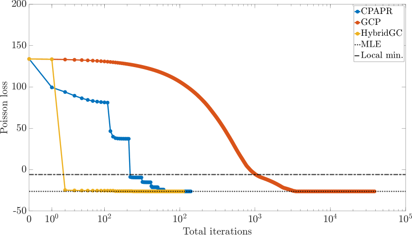
(a) Trial where all methods converged to the MLE.

(b) Trial where only HybridGC converged to the MLE.

Figure 1: Examples of two types of behaviors of traces of loss function values for GCP, CPAPR, and HybridGC on LowRankSmall.

A few remarks:

• Our results demonstrate the benefit of performing some amount of stochastic search followed by deterministic search. Owing to performing one outer iteration of stochastic search, HybridGC quickly identified the basin of attraction of the MLE and converged before GCP and CPAPR in both trials, even in the case where the standalone method converges to a local minimizer that is different from the MLE. The iteration histories of GCP and CPAPR are consistent with results from prior work on small tensors [56]. A further research direction may study the effect of looser convergence tolerances on the amount of computation or accuracy.

• The shared behavior among all methods of making only incremental progress before finally converging is a feature of the theoretical convergence properties of each method. Mathematically, CPAPR (in the case of MU) and the deterministic stage of HybridGC converge sublinearly in the basin of attraction to the MLE; GCP (in the case of Adam) converges only linearly at best. See [56, Table 1] for details. However, the stagnation of HybridGC in Fig. 1(b) near the local minimizer is indicative of a swamp [54]. We leave it to future work to compare HybridGC with methods designed to avoid swamps.

Table 1 presents average behavior about algorithm effectiveness as estimates of the probability that each method computed the empirical MLE with relative error Eq. 6 less than $\epsilon$ for LowRankSmall and MedRankLarge. Viewing the average behavior, we conclude the following:

• For the small dataset with low rank (LowRankSmall), HybridGC and CPAPR had comparable precision at all levels of accuracy. Additional work may be conducted to determine if the differences are statistically significant.

• HybridGC was never worse than GCP or CPAPR, since it interpolates the two methods. At high accuracy on the large dataset with medium rank (MedRankLarge), HybridGC had a higher probability of getting close to the empirical MLE.

• Even for small input tensors with low rank, GCP was virtually incapable of resolving the MLE beyond a coarse-grain approximation. The situation was worse for larger tensors with more components.

Table 1: Estimate of probability each method computes a solution within $\epsilon$-radius of approximate global optimizer.

(a) LowRankSmall dataset (110K trials).

$\epsilon$	CPAPR	GCP	HybridGC
$10^{-1}$	0.963	0.963	0.967
$10^{-2}$	0.963	0.963	0.967
$10^{-3}$	0.963	0.879	0.967
$10^{-4}$	0.963	0.003	0.967

(b) MedRankLarge dataset (100 trials).

$\epsilon$	CPAPR	GCP	HybridGC
$10^{-1}$	1.00	1.00	1.00
$10^{-2}$	0.46	0.04	0.46
$10^{-3}$	0.03	0.00	0.17
$10^{-4}$	0.00	0.00	0.01

5.5 Comparison as algebraic structures

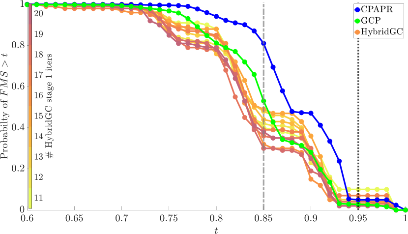
(a) 11 to 20.

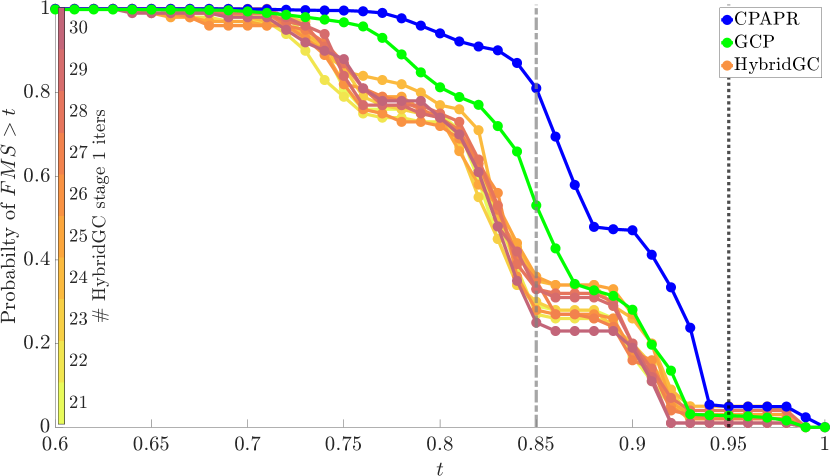
(b) 21 to 30.

(c) 31 to 40.

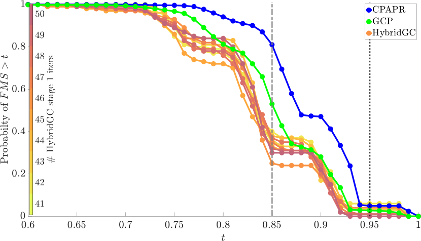
(d) 41 to 50.

(e) 51 to 60.

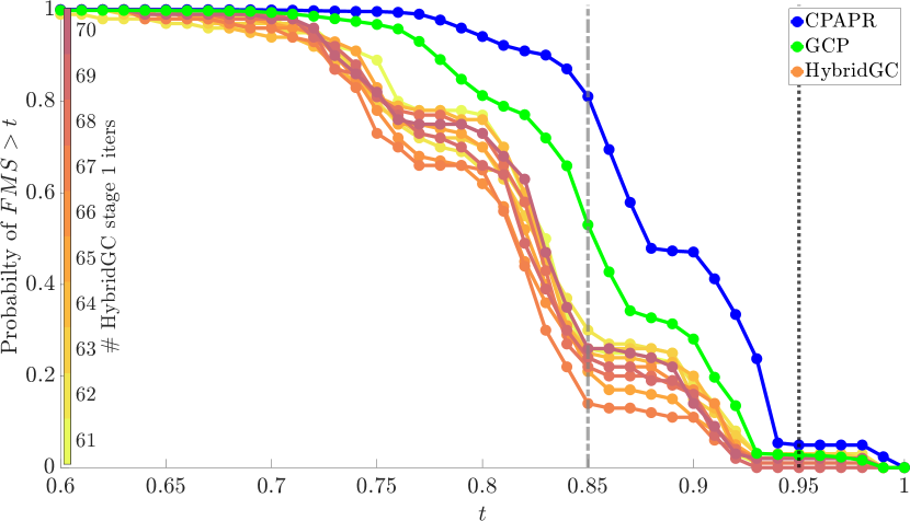
(f) 61 to 70.

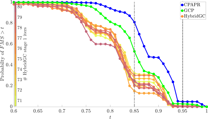
(g) 71 to 80.

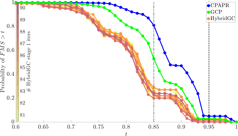
(h) 81 to 90.

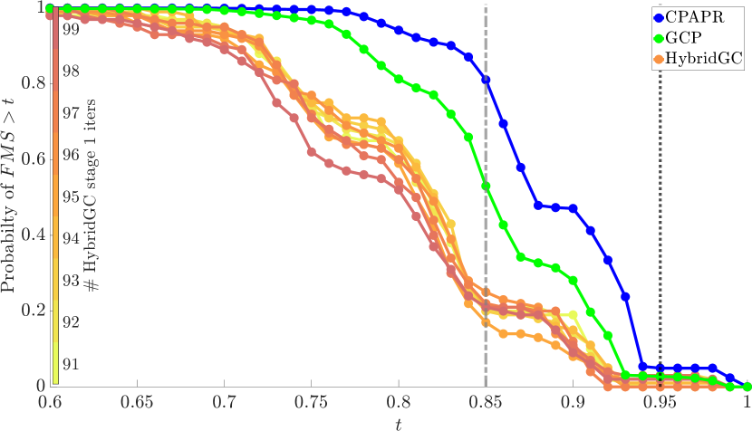
(i) 91 to 99.

Figure 8: Factor match scores between CP models computed with HybridGC, CPAPR-MU, and GCP-Adam and the approximate global optimizer, $\bm{\mathscr{\widehat{M}}}_{\mathcal{S}}^{*}$. The dash-dot gray vertical lines and dotted black vertical lines denote the levels of “similar” and “equal” described in [52]. Colormaps scaled for clarity.

Next, we evaluate HybridGC as a method for computing an approximate low-rank basis to the global optimizer. We calculated the fraction of trials with $\operatorname{FMS}$ greater than $t$ Eq. 10 for GCP and CPAPR, i.e., $\Psi(\bm{\mathscr{\widehat{M}}}_{\mathcal{S}}^{*},\mathcal{S}_{G},t)$ and $\Psi(\bm{\mathscr{\widehat{M}}}_{\mathcal{S}}^{*},\mathcal{S}_{C},t)$, with $t\in[0,1]$. We repeated this calculation for HybridGC, i.e., $\Psi(\bm{\mathscr{\widehat{M}}}_{\mathcal{S}}^{*},\mathcal{S}_{H},t)$, and grouped the results by the number of outer iterations taken by the first stage of HybridGC. Figure 2 presents these results for GCP, CPAPR, and HybridGC (up to 10 outer iterations of GCP). See Fig. 8 in Appendix D for supplementary results. Since all curves showed the same behavior for $t<0.6$, we report values for $t\in[0.6,1]$.

HybridGC tended to have a higher likelihood than GCP or CPAPR in finding a low-rank basis equal to the empirical MLE when FMS $>0.95$, which is considered high accuracy. This figure provides numerical evidence that HybridGC—parameterized as a small amount of stochastic search ($\sim 10$ outer iterations) followed by deterministic search—was superior to GCP and CPAPR by themselves in computing high accuracy models (solutions with FMS greater than 0.95).

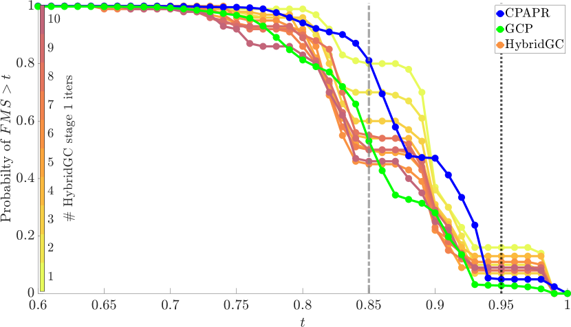
Figure 2: Factor match scores between CP models computed with HybridGC, CPAPR-MU, and GCP-Adam and the approximate global optimizer, $\bm{\mathscr{\widehat{M}}}_{\mathcal{S}}^{*}$. The dash-dot gray vertical lines and dotted black vertical lines denote the levels of “similar” and “equal” described in [52].

6 Restarted CPAPR with SVDrop

We observed in Section 5.3 that there are situations where HybridGC converges to the MLE but a standalone method like CPAPR does not, and vice versa. The standalone method may converge to a minimizer far from the MLE despite having started from the same point. The standalone method may also converge to the MLE whereas HybridGC converges to some other minimizer. Thus it is necessary to characterize the situations that end in algorithm failure so that we may explain these seemingly conflicted outcomes. Since it is easier to reason about a deterministic search path, we focus on sources of failure in CPAPR and leave a similar study of GCP for future work. CPAPR is also interesting because of its high success rate, meaning it is sometimes feasible to examine all failed trials exhaustively. Furthermore only a small number of parameters affect the search path of CPAPR in [18, Alg. 3]. Another motivator for the work presented here is that CPAPR is used to refine the solution in HybridGC, thus understanding convergence properties is important. Taking these factors into account, CPAPR is a good candidate to analyze in order to understand why and when local methods fail for Poisson CPD.

The starting point for our analysis is the use of standard linear algebra tools that are well-understood to identify patterns that explain distinct convergence behaviors. We are motivated by the following reasoning. Tensor decompositions are multilinear objects but the algebraic operators and computational kernels that factorize tensors in popular CP algorithms are linear, e.g., matricizations of tensor modes, objective function evaluation, gradient computations, and so on. Examining the mode unfoldings of the model between inner iterations could reveal latent patterns so that we may witness the action of the linear operators on the entire multilinear object. In fact, Golub and Van Loan, in their seminal work Matrix Computations [26], inadvertently foreshadowed this research direction when they wrote: “Hidden structures within a tensor dataset can sometimes be revealed by discovering patterns within its unfoldings”.

This work uncovers an unexplored connection between the convergence behavior of CPAPR and the spectral properties of the mode unfoldings as the variables of the model change along the search path. We demonstrate the utility of our analysis by showing empirically that spectral information contained in mode unfoldings may reveal otherwise hidden patterns about convergence to local minimizers that we observe to be rank-deficient. Specifically we define a rank-deficient CPD solution to be one that is comprised of one or more factor matrices with column rank less than the requested rank $R$.

6.1 Related work

Early work by Kruskal et al. [50] studied two-factor degeneracies (2FD), where two components of a CPD model are highly correlated in all three modes. Mitchell and Burdick introduced a test for 2FD in [54], which uses an early definition of FMS to identify 2FD between successive iterates. More recent work [25] add constraints (e.g., orthogonality constraints, ridge regression, SVD penalty) to the problem to avoid 2FD. To the best of our knowledge, the connection between rank-deficient solutions (rather than 2FD) and the spectra of mode unfoldings has never been studied with the goal of understanding the convergence behavior of Poisson CPD algorithms specifically nor any CPD algorithms in general.

6.2 Road map

We first motivate our analysis by observing a previously unreported problem and reasoning as to its implications in Section 6.3. In Section 6.4, we characterize this problem and demonstrate empirically that: 1) the problem occurs frequently when computing the Poisson CPD for a small synthetic dataset and 2) it can be identified using spectral information of the mode unfoldings. In Section 6.5, we develop a heuristic called SVDrop that leverages spectral information to identify this problem. We then present a novel variant of the CPAPR algorithm called Restarted CPAPR with SVDrop (Algorithm 2) that automatically restarts when a rank-deficient solution is detected. In Section 6.6, we present experimental evidence that Restarted CPAPR with SVDrop improves the probability of convergence to the MLE with an acceptable increase in computational cost.

6.3 The drawback of extra (or too few) inner iterations

Chi and Kolda’s CPAPR paper [18] included a section titled “the benefit of extra inner iterations”. Their conclusion was that although the maximum allowable number of inner iterations $l_{max}$ “does not significantly impact accuracy… increasing $l_{max}$ can decrease the overall work and runtime”. They drew their conclusion from the mean and median factor match score (FMS) between the model and the “true solution”. However, this definition of accuracy is incomplete since it ignores error estimators on the loss function. Instead, our definition of accuracy includes both the objective function value and expected convergence behavior over many trials. Ultimately, we reach the opposite conclusion: the maximum allowable number of inner iterations can significantly impact algorithm accuracy. Subsequently, overall work and runtime are also affected. For instance, we observed situations where, from one fixed starting point, CPAPR would converge to different minima for increasing values of $l_{max}$ in an alternating fashion: to the MLE for some value of $l_{max}$, then to a different minimizer for a larger value, and again to the MLE for an even larger value of $l_{max}$. In some cases, this alternating pattern repeated multiple times. This behavior was not rare. In one trial from 3,677 starting points, we observed some type of alternating convergence pattern in 3,180 instances (86.4%). In general, characterizing the sensitivity of CPAPR to $l_{max}$ is complicated.

Figure 3 demonstrates one example empirically where the effect of extra inner iterations counters Chi and Kolda’s claim. The upper plot shows the trace of the objective function value over the total iteration history when $l_{max}=4$. CPAPR converges to the MLE (black dash-dot line) in 116 iterations. The lower plot is taken from the same initial point except $l_{max}=5$. Surprisingly, CPAPR converges to a KKT point far from the MLE (black dotted line) in 887 iterations. We will return to this case throughout the rest of this section, so we will refer to it as the exemplar trial.

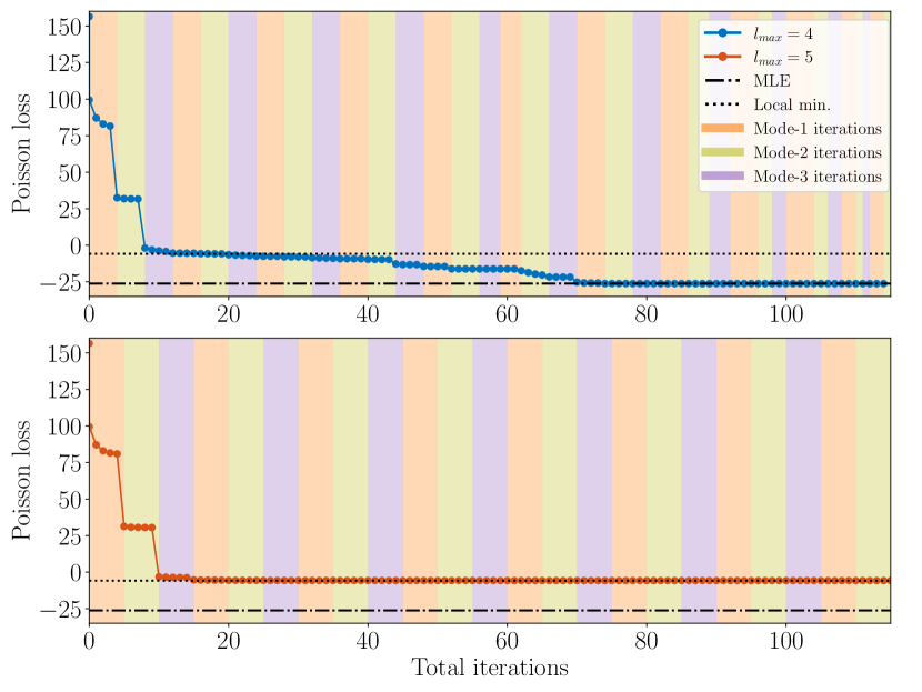
Figure 3: Traces of objective function values for the exemplar trial: two decompositions computed by CPAPR starting from the same initial guess but with different numbers of maximum allowable inner iterations per mode. With $l_{max}=4$ maximum inner iterations (top), CPAPR converges to the MLE, versus $l_{max}=5$ (bottom), which converges to a different minimizer. The $x$-axis is given in terms of the total number of iterations, so optimizations by mode are differentiated by vertical blocks of color. For clarity, the $x$-axes in both plots are sized to the total number of iterations of the top case (116). The bottom case continues up to 887 total iterations and does not improve.

Incremental changes to this parameter can result in drastically different outcomes. In experimentation, we frequently observe that, for the first several outer iterations, CPAPR tends to max out the number of inner iterations in each mode without converging. This led to the conclusion that early iterations are especially critical and sensitive to $l_{max}$. Figure 4 presents a conceptual model explaining the situation. The contour plot reflects the minima (in blue) and maxima (in brown) of a $d=2$ problem. Darker shades reflect more extreme values. The $x$- and $y$-axes represents search paths in the directions of the second and first modes, respectively. The green, magenta, and red lines represent the search paths of CPAPR from the same initial starting point (yellow circle) but with different values for $l_{max}$. The magenta and red paths allow too many or too few inner iterations and converge to local minimizers. The green path allows the “Goldilocks” amount—this choice leads to the MLE. We will show that our novel analysis can differentiate between the green path and the magenta and red paths at runtime.

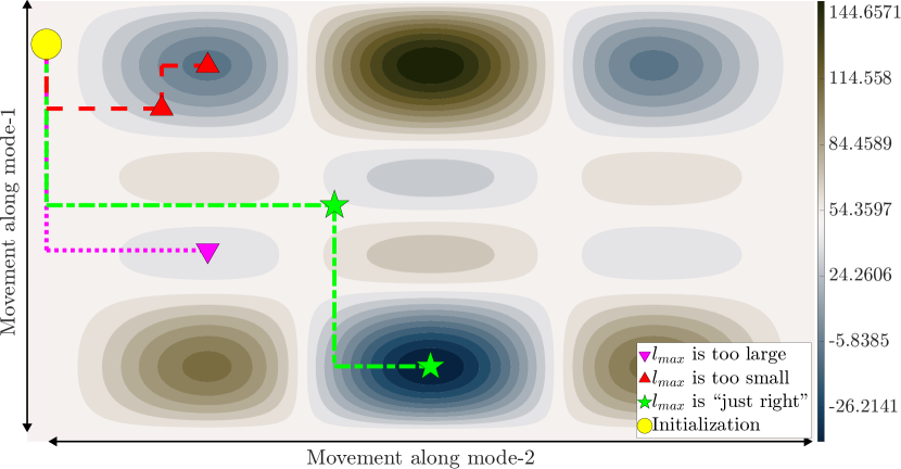
Figure 4: The contour plot illustrates how convergence depends on the number of inner iterations in the search direction for a 2D problem. Blue represents minima and brown represents maxima; darker shades are more extreme values than lighter shades. From the same starting initialization, CPAPR is run with three different values for inner iterations $l_{max}$: 1) the “Goldilocks” amount that leads to the MLE; 2) too few or 3) too many inner iterations, which both lead to different minimizers.

6.4 Spectral properties identify rank-deficient solutions

By analyzing the singular values of each mode unfolding, we can see critical changes to the model tensor that are otherwise hidden. In particular, we consider the $R$-th largest singular value when the requested decomposition rank is $R$. Figure 5(a) shows the values of the third largest singular value (since $R=3$) of each of the mode unfoldings over the iteration history. The solid lines are when $l_{max}=4$; they correspond to the case when CPAPR converges to the MLE. The dotted lines are when $l_{max}=5$; they correspond to the case when CPAPR converges to a different local minimizer. Both trials iterated from the same initial guess. The critical observation is that the $R$-th singular value in mode-1 when $l_{max}=5$ inner iterations are taken per outer iteration (blue dotted line) is driven below machine precision, resulting in a rank-deficient solution. The rank-deficient solution is a KKT point, but it is not the MLE. Ceteris paribus, the search path that leads to it is determined by $l_{max}$.

At present this analysis of success versus failure is only possible by examining the singular values of the mode unfoldings. By contrast, the values of the tensor model factor weights $\lambda$ in Eq. 3 show no obvious link between the search path and convergence behavior. Figure 5(b) displays the $\lambda$ values of the CP model at each iteration for both values of $l_{max}$ in the exemplar trial. The $\lambda_{1}$ and $\lambda_{3}$ values (blue and yellow, respectively) became nearly identical when the number of inner iterations taken per outer iteration was $l_{max}=5$. This occurred at nearly the same time the mode-1 $R$-th singular value started to drop drastically. It remains unclear whether this behavior may indicate convergence to a rank-deficient solution or if it is just a coincidence. We did not observe a similar pattern in the $\lambda$ weights in a sample of other trials with similar behaviors in the singular values. The behavior also is not explained by standard techniques in optimization, e.g., unsatisfied convergence criteria, or machine learning, e.g., large gradient norms. The $R$-th largest singular value of the mode-1 unfolding is a pronounced indicator of convergence to a rank-deficient solution.

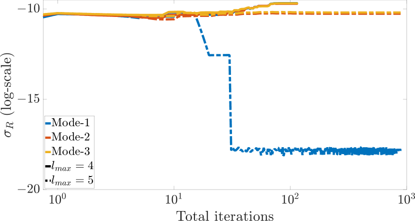
(a) Analyzing the $R$-th largest singular value of each mode yields an explicit signal indicating convergence to a rank-deficient solution.

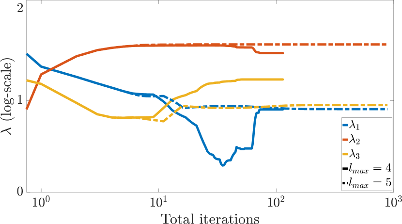
(b) It is unclear whether the $\lambda$-weights provide a useful heuristic for determining convergence to the MLE versus a rank-deficient solution.

Figure 5: Traces of singular values and $\lambda$ weights for the exemplar trial on LowRankSmall. Figure 5(a): $R=3$-rd largest singular value of each mode unfolding after each update. Figure 5(b): the $R$ $\lambda$-values maintained by CPAPR in each iteration.

We observed this behavior in most cases. Recall from Table 1(a) that CPAPR converged to the MLE in 106,215 of 110,266 trials ($\widehat{P}(\epsilon=10^{-4})=0.963$). For a random sample of 10,000 of these trials, the Poisson CP models were not rank-deficient: the $R$-th largest singular value when CPAPR terminated was typically far from machine precision ($4.449$ on average). By contrast, in 4,020 of the 4,051 trials (99.235%) where CPAPR converged to a different KKT point, we found that the $R$-th largest singular value in mode-1 when CPAPR terminated was on the order of double precision machine epsilon (i.e., $\approx 2.2204\times 10^{-16}$). Thus we describe these models as rank-deficient: when the $R$-th largest singular value in one or more modes is numerically close to 0 (i.e., near or below machine precision) so that the column rank of these mode unfoldings is less than $R$. We can reasonably conclude that there is a strong connection between rank-deficient solutions and KKT pointers that are not the MLE.

6.5 Restarted CPAPR with the SVDrop heuristic

Upon closer examination of the traces from the rank-deficient search path in Fig. 5(a), we notice that the $R$-th largest singular value in mode-1 drops dramatically between the 29th and 30th iteration. (In this case, $l_{max}=5$, so the 30th total iteration is the first inner iteration on mode-1 of the 3rd outer iteration.) To be precise, the gap ratio of the $R$-th largest singular value from the mode-1 unfolding between iterations 29 and 30 is $\sigma_{(1)}[R]^{(29)}/\sigma_{(1)}[R]^{(30)}\approx 3.6\times 10^{10}$. Considering all of the failed trials, the maximum gap ratio was $1.55\times 10^{12}$ on average, the median of the maximum gap ratios was $2.95\times 10^{6}$, and the median iterate where it was observed was the 30th iteration. Analogous to the indication of numerical instability by large condition number, we interpret a large gap ratio between successive iterates as indicative of a search path that will converge to a rank-deficient solution. Therefore, large gap ratio may serve as a reliable heuristic to determine whether the current search path should be accepted or rejected. This observation informs our solution in Algorithm 2. Before we present the method in full, two core concepts remain to be discussed: 1) the SVDrop heuristic and 2) Restarted CPAPR.

Regardless of the method chosen to compute the spectral properties of the tensor mode unfoldings, calculating the gap ratio between successive iterates will add non-trivial costs due to the SVD computation. Additionally, it is not even clear whether the gap ratio needs to be computed after every update. To mitigate incurring excessive computational cost, we propose the SVDrop heuristic in a new subproblem for an extended CPAPR algorithm.

6.5.1 Procedure

The inputs to the subproblem algorithm are:

1. the maximum number of inner iterations, $l_{max}\in\mathbb{N}_{>0}$;

2. the number of SVDrop inner iterations between successive models for computation of their spectral properties, $\tau\in\mathbb{Z}_{+}$; and,

3. a maximum threshold for the gap ratio indicating an acceptable search path, $\gamma\in\mathbb{R}_{+}$.

While the model is not converged, we compute a rank-$R$ decomposition with CPAPR and improve the model fit with multiplicative updates. Every $\tau$ inner iterations, we compute the spectral properties of the current model (i.e., the singular values of the mode unfoldings). If the gap ratio between the current model and the checkpointed model, computed from their spectral properties, is smaller than $\gamma$, then we accept the search path, checkpoint the model, and continue iterating. When the gap ratio is greater than $\gamma$, the SVDrop heuristic indicates that the search path will converge to a rank-deficient solution and we reject it, since to otherwise continue likely will waste a great deal of computation, as seen in Fig. 1 and Fig. 5. A simple option is to restart: discard the work done up to now, randomly choose a new starting point in the feasible domain of the optimization problem, and recompute. Restarting, taken together with the SVDrop heuristic, is the idea behind our new method, Restarted CPAPR with SVDrop, presented in Algorithm 2 and Algorithm 3. The exposition follows the template of the ideal version of CPAPR [18, Algs. 1–2].

6.5.2 Additional considerations

First, we reset the counter of SVDrop inner iterations before the first inner iteration of a mode, since we observed that the singular values of the unfoldings of the modes that are held fixed change very little between iterations. A consequence is that the number of SVDrop inner iterations should always be less than or equal to the maximum number of inner iterations, i.e., $\tau\leq l_{max}$. Second, the gap ratio tolerance $\gamma$ should be sufficiently large. We used $\gamma=10^{6}$ in our numerical experiments but it is unknown if this value generalizes to other problems. Third, the update step Line 10 in Algorithm 3 is for exposition; it can be performed implicitly on $\bm{\mathscr{M}}$ efficiently in software.

Algorithm 2 Restarted CPAPR algorithm with SVDropSubproblem).

1:Let $\bm{\mathscr{X}}$ be a tensor of size $I_{1}\times\dots\times I_{d}$.

2:User input:

• $R$: Number of components in low-rank approximation

• $l_{max}$: Maximum number of inner iterations per outer iteration

• $\tau$: Number of SVDrop inner iterations to perform

• $\gamma$: Tolerance for identifying rank-deficiencies (e.g., $10^{6}$)

3:$\texttt{restart}\leftarrow\text{true}$

4:repeat  {SVDrop}

5:     if $(\texttt{restart})$ then

6:         $\bm{\mathscr{M}}\leftarrow\textsc{GenerateRandomGuess}([I_{1},\ldots,I_{d}],R)$      

7:     repeat  {OuterIteration}

8:         for $n=1,\ldots,d$ do

9:              $\bm{\mathbf{\Pi}}\leftarrow\left(\bm{\mathbf{A}}^{(d)}\odot\dots\odot\bm{\mathbf{A}}^{(n+1)}\odot\bm{\mathbf{A}}^{(n-1)}\odot\dots\odot\bm{\mathbf{A}}^{(1)}\right)^{T}$

10:              $\left[\bm{\mathbf{B}},\texttt{restart}\right]\leftarrow\textsc{SVDropSubproblem}(\bm{\mathscr{M}},\bm{\mathbf{\Pi}},R,n,l_{max},\tau,\gamma)$

11:              if $(\texttt{restart})$ then

12:                  break $\triangleright$ Break out of {OuterIteration}.               

13:              $\bm{\mathbf{\lambda}}\leftarrow\bm{\mathbf{e}}^{T}\bm{\mathbf{B}}$

14:              $\bm{\mathbf{A}}^{(n)}\leftarrow\bm{\mathbf{B}}\bm{\mathbf{\Lambda}}^{-1}$          

15:     until convergence {OuterIteration}

16:until convergence {SVDrop}

Algorithm 3 Subproblem solver for Algorithm 2 with SVDrop heuristic.

1:function SVDropSubproblem($\bm{\mathscr{M}},\bm{\mathbf{\Pi}},r,k,l_{max},\tau,\gamma$)

2:     $t\leftarrow 0$

3:     $\sigma_{r}\leftarrow\text{svd}(\bm{\mathbf{M}}_{(k)})[r]$ $\triangleright$ $r$-th largest singular value of $\bm{\mathbf{M}}_{(k)}$.

4:     $\bm{\mathbf{B}}\leftarrow\bm{\mathbf{A}}^{(k)}\bm{\mathbf{\Lambda}}$

5:     for $l=1,\ldots,l_{max}$ do

6:         $t\leftarrow t+1$

7:         $\bm{\mathbf{\Phi}}\leftarrow\left(\bm{\mathbf{X}}_{(k)}\oslash\left(\bm{\mathbf{B}}\bm{\mathbf{\Pi}}\right)\right)\bm{\mathbf{\Pi}}^{T}$

8:         $\bm{\mathbf{B}}\leftarrow\bm{\mathbf{B}}\ast\bm{\mathbf{\Phi}}$

9:         if $(t=\tau)$ then

10:              $\bm{\mathbf{\lambda}}\leftarrow\bm{\mathbf{e}}^{T}\bm{\mathbf{B}},\,\bm{\mathbf{A}}^{(k)}\leftarrow\bm{\mathbf{B}}\bm{\mathbf{\Lambda}}^{-1}$ $\triangleright$ Update $\bm{\mathscr{M}}$ with $\bm{\mathbf{B}}$.

11:              $\sigma_{r}^{(l)}\leftarrow\text{svd}(\bm{\mathbf{M}}_{(k)})[r]$

12:              if $(\sigma_{r}/\sigma_{r}^{(l)}>\gamma)$ then

13:                  return $[\bm{\mathbf{B}},\texttt{true}]$ $\triangleright$ $\operatorname{rank}(\bm{\mathscr{M}})<r$; forces a restart in Algorithm 2.               

14:              $\sigma_{r}\leftarrow\sigma_{r}^{(l)}$

15:              $t\leftarrow 0$               

16:     return $[\bm{\mathbf{B}},\texttt{false}]$ $\triangleright$ $\operatorname{rank}(\bm{\mathscr{M}})=r$; does not force a restart in Algorithm 2.

6.6 Numerical experiments

To evaluate Restarted CPAPR with SVDrop, we selected 14,051 random initializations for LowRankSmall from the experiments in Section 5.3: the random sample of 10,000 starts where CPAPR converged to the MLE that we mentioned previously plus the 4,051 starts where CPAPR converged to a different KKT point. We computed rank $R=3$ CP decompositions using CPAPR with Multiplicative Updates starting from each point. We increased the number of SVDrop inner iterations as $\tau\in\{0,\ldots,10\}$ but kept all other parameters identical to the experiments in Section 5.3. A value $\tau=0$ indicates that SVDrop was not used and that CPAPR was not restarted at any iteration.

6.6.1 Probability of convergence

In the previous experiments using CPAPR without any restarts, the total number of trials that did not converge to the MLE at the level of $\epsilon=10^{-4}$ was 4,051 of 110,266 ($1-\widehat{P}_{MLE}(10^{-4})=0.037$; see Table 1(a)). Table 2 reports the total number of trials that: 1) converged to the MLE, 2) converged to some other KKT point, or 3) did not converge to any KKT point using this set of 4,051 initial starts. Convergence was calculated as in Eq. 6 at the level of $\epsilon=10^{-4}$ for each value of $\tau$. Of these, 3,905 converged to some other KKT point and 146 did not converge to any KKT point when $\tau=0$. Our method improved on this in all cases. It is interesting to note that the probabilities of convergence to a different KKT point and failure to converge to any KKT point were higher when $\tau\geq 6$. We defer further discussion on this point to Section 6.7 since we will provide additional results that will help us reason about this behavior and allow us to make suggestions with more context.

In the best case, when the number of SVDrop inner iterations was $\tau=2$, Restarted CPAPR with SVDrop recovered the MLE in all but two trials ($\widehat{P}_{MLE}(10^{-4})=0.9995$). In these cases, SVDrop did not converge to a KKT point. Instead CPAPR oscillated near some other local minimizer—perhaps a saddle point. Figure 6 demonstrates that the failure of SVDrop in these two instances was due to setting the gap ratio tolerance $\gamma$ too large (red curves). In both plots, the gap ratio was always less than the choice of the tolerance in our experiments ($\gamma=10^{6}$). When set appropriately, e.g., $\gamma=8\times 10^{3}$ (blue curves), Restarted CPAPR with SVDrop converged. Note that the traces for the red and blue curves were identical until the gap tolerance has been exceeded in the blue case. This triggered a restart, so that the iteration histories diverged. Observe that the trial on the right restarted twice when $\gamma=8\times 10^{3}$. Algorithm 2 will always restart until convergence to a KKT point that is not rank-deficient.

Table 2: Convergence results of Restarted CPAPR with SVDrop: the number of trials that converged to the MLE, converged to some other KKT point, or did not converge to a KKT point. The initial guesses were the set of starts from previous experiments where CPAPR without restarting (i.e., $\tau=0$) did not converge to the MLE (number of starts $N=4051$). Converged means the solution satisfied the KKT-based CPAPR convergence criterion to tolerance $10^{-15}$.

		SVDrop inner iterations $\tau$
Converged	Minimizer	0	1	2	3	4	5	6	7	8	9	10
Yes	MLE	0	4024	4049	4035	4028	4029	3906	3970	3983	3990	3998
Yes	Other KKT point	3905	0	0	0	0	0	102	43	31	24	20
No	-	146	27	2	16	23	22	43	38	37	37	33

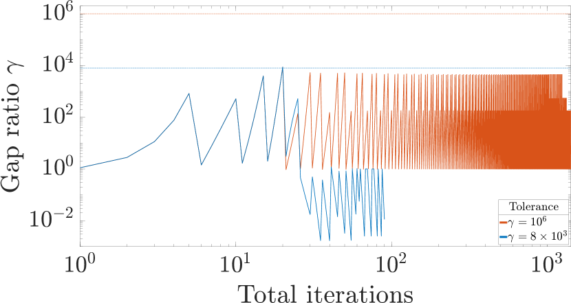
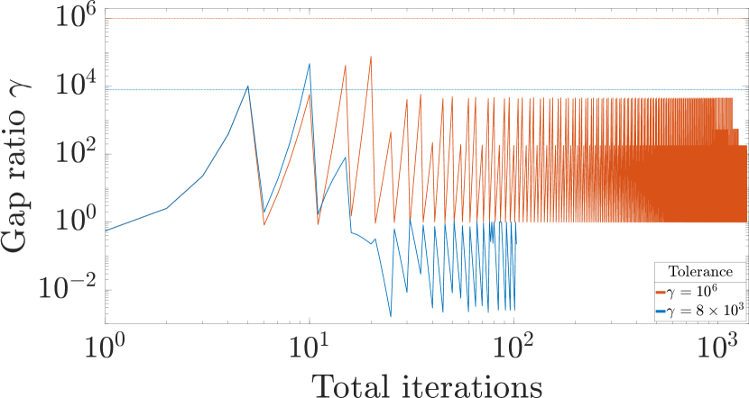
Figure 6: Two trials demonstrating the sensitivity of SVDrop to $\gamma$. Starting from points where CPAPR without restarting (i.e., $\tau=0$) was known to converge to the MLE, SVDrop failed to converge to any KKT point when $\gamma$ was set too large (red). When $\gamma$ is too large, SVDrop may fail to recognize rank deficiency and CPAPR may stagnate near a local minimizer that is not a KKT point. When set appropriately (blue), SVDrop converged to the MLE.

6.6.2 Computational cost

The formulae to compute computational costs in FLOPS are provided in Appendix B. In the best case ($\tau=2$), the cost of Restarted CPAPR with SVDrop was 7.04$\times$ higher than CPAPR without restarting ($\tau=0$). Although the cost of converging to the MLE using Restarted CPAPR with SVDrop was more expensive than CPAPR without restarting, it may be possible to converge to the MLE with higher probability—$\widehat{P}_{MLE}(10^{-4})=0.9995$ versus $\widehat{P}_{MLE}(10^{-4})=0.963$—with the extra work.

6.6.3 Caveats

Although our results were promising, we caution that our approach may not always improve on CPAPR without restarting. There appears to be a “Goldilocks” range for the gap ratio: too large $\gamma$ may decrease the probability that rank-deficient solutions are identified and too small $\gamma$ may trigger unwanted restarts.

Choosing $\gamma$ too large

Starting from the random sample of 10,000 points where CPAPR without restarting converged to the MLE in previous experiments, SVDrop occasionally performed worse. When the number of SVDrop inner iterations was $\tau=1$, 34 trials did not converge to a KKT point. When the number of SVDrop inner iterations was $\tau=8$, one trial converged to a KKT point that was not the MLE. In that trial, a restart was triggered when the gap ratio was greater than $10^{6}$. However, two gap ratios, which were large ($>2\times 10^{4}$) but below the threshold, were missed due to the tolerance having been set too large.

Choosing $\gamma$ too small

When starting from points known to converge to the MLE without restarting (i.e., $\tau=0$), it is possible that SVDrop could misclassify a solution as rank-deficient and restart from a new initial guess, which might needlessly increase the work expended. We consider this unwanted behavior since minimal computational cost, in addition to accuracy, is a desired characteristic of our algorithm. Figure 7 shows estimated probabilities that SVDrop would trigger an unwanted restart for a range of gap ratios $\gamma$. The implication is that choosing $\gamma$ to be too small may hurt performance.

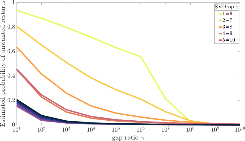
Figure 7: For trials that were known to converge to the MLE without using SVDrop, this figure reflects the estimated probabilities that SVDrop would trigger an unwanted restart for a range of gap ratios $\gamma$.

6.7 Discussion

The results for SVDrop presented here are limited to a small exemplar. We discuss below several questions that should be addressed before conclusions about the general efficacy of SVDrop can be considered.

6.7.1 Connections between $\tau$, $\gamma$, and $l_{max}$

It is possible that the number of SVDrop steps should be bounded by half the number of inner iterations, $\tau\leq\lfloor l_{max}/2\rfloor$. The reason being that there is a correspondence between $\tau$, $l_{max}$, and the number of times the gap ratio is computed per set of inner iterations. To see this, suppose $l_{max}=10$ and $\tau=6$. If not converged when $l=6$, then the gap ratio would be computed only once for that mode; any additional changes to the model variables beyond that inner iteration would not be captured by SVDrop. Since rank-deficiency might only be indicated by the singular values of only one mode, as we observed in Figure 5(a), it may not be apparent that the model had been driven even closer to a rank-deficient solution while the remaining modes were being optimized. If $\tau=5$, then the gap ratio would be computed twice: first when $l=5$ and again when $l=10$. In this case, we would not miss critical changes. Thus it is possible that the gap ratio should be computed at least twice per set of inner iterations. Two possible options are to set $\tau=\lfloor l_{max}/2\rfloor$ or to compute $\gamma$ when $l=l_{max}$. On the other hand, Fig. 7 shows that the estimated probability of unwanted restarts is less when $\tau\geq 6$ than when $\tau\leq 5$. We speculate that choices of $\tau$ and $\gamma$ are highly-coupled when considering both the probability of convergence to the MLE and the probability of unwanted restarting. We leave this investigation to future work.

6.7.2 Swamps

In future work, we will explore rank-deficiency more systematically for local minimizers of Poisson CPD problems to better understand the general applicability of our SVDrop approach. For example, in Fig. 3, the CP model appears to be in a swamp close to some local minimizer before emerging to converge to the MLE. One direction open to future work is to compare SVDrop with methods for avoiding 2FD such as those in [25].

6.7.3 Efficient computation of gap ratios

Black-box solvers, e.g., those built on LAPACK xGES*D[5], compute all of the singular values of the matrix. Iterative methods, such as subspace iteration or Krylov methods, may be a more practical choice for computing the gap ratio due to the (relatively) small number of nonzero entries in each unfolding (This is a consequence of the CPAPR algorithm design that drives elements toward zero.) Iterative methods are also useful when only a small number of singular values are needed and are amenable to sparse data structures. While it is less straightforward to characterize the computational costs and other trade-offs of iterative methods, it is worth investigating their role in future work.

7 Conclusions

We presented two new methods for Poisson canonical polyadic decomposition: HybridGC and Restarted CPAPR with SVDrop.

7.1 HybridGC

Our method can minimize low-rank approximation error with high accuracy relative to GCP-Adam and CPAPR-MU while reducing computational costs. Since HybridGC was run in our experiments with a far stricter computational budget than GCP-Adam and CPAPR-MU, we argue that HybridGC can be more computationally efficient. The implication is that the performance gain allows even more multi-starts, and subsequently, a greater number of high accuracy approximations. Furthermore, our contribution is a new method that interpolates two very different algorithms.

7.2 Restarted CPAPR with SVDrop

Our method identifies rank-deficient solutions with near-perfect accuracy and has the highest likelihood of finding the MLE in our experiments. A corollary is that our algorithm almost always avoids an entire class of minimizers that are different from the MLE. Our experimental results demonstrate this empirically with conservative budgets for both restarting and total iteration, alongside other untuned parameters. Provided more generous allotments and proper tuning, we expect SVDrop to always identify rank-deficient solutions in the limit of multi-starts.

7.3 Parameter tuning

Unlike SVDrop, HybridGC lacks a mechanism for changing its search path. Assuming a pattern behavior exists, it is essential that further algorithm development uncovers a diagnostic to identify it. Otherwise, HybridGC will remain reliant on costly ad hoc parameter tuning by the user. Convergence and the computational cost of Restarted CPAPR with SVDrop both depend on the complex interplay of search parameters, which is not well-understood. Although we provided sensible values and rationalized upper bounds on some parameters, it remains an open question as to how sensitive SVDrop is to parameter variability. It is essential to better understand this interplay since SVDrop can be prohibitively expensive when it does fail. Fortunately, this is rare.

Appendix A LowRankSmall synthetic data tensor and empirical maximum likelihood estimator from numerical experiments

Sparse Tensor 1: Synthetic data tensor LowRankSmall used in experiments in Section 5.3.

⬇

sptensor %% tensor type

3 % number of dimensions

4 6 8 % sizes of dimensions

17 % number of nonzeros

1 4 1 1 % start of sparse tensor data: <mode-1-index> <mode-2-index> <mode-3-index> <value>

1 4 6 5

1 4 7 9

1 6 6 1

1 6 7 1

2 1 2 6

2 1 4 5

2 1 8 3

2 4 4 1

2 5 2 1

2 6 2 6

2 6 4 8

2 6 8 3

4 1 8 4

4 2 1 1

4 2 8 2

4 5 8 1

MLE Kruskal Tensor 2: Kruskal tensor empirical maximum likelihood estimator (MLE) of LABEL:data:hybrid-gc:low-rank-small-sptensor computed in experiments in Section 5.3. The empirical MLE is the solution with the smallest Poisson loss from among 110,226 random starts.

⬇

ktensor %% tensor type

3 % number of dimensions

4 6 8 % sizes of dimensions

3 % number of components

3.2999999999999986e+001 1.7000000000000004e+001 8.0000000000000000e+000 % lambda values

matrix %% 1st factor matrix

2 % number of dimensions

4 3 % sizes of dimensions

0.0000000000000000e+000 1.0000000000000000e+000 0.0000000000000000e+000 % start of data

1.0000000000000000e+000 0.0000000000000000e+000 7.7243827424339032e-017

0.0000000000000000e+000 0.0000000000000000e+000 0.0000000000000000e+000

9.1691651618349857e-046 0.0000000000000000e+000 1.0000000000000000e+000

matrix %% 2nd factor matrix

2 % number of dimensions

6 3 % sizes of dimensions

4.2424242424242420e-001 0.0000000000000000e+000 5.0000000000000033e-001 % start of data

9.8952534188649872e-233 0.0000000000000000e+000 3.7499999999999983e-001

0.0000000000000000e+000 0.0000000000000000e+000 0.0000000000000000e+000

3.0303030303030307e-002 8.8235294117647056e-001 0.0000000000000000e+000

3.0303030303030307e-002 0.0000000000000000e+000 1.2499999999999993e-001

5.1515151515151525e-001 1.1764705882352941e-001 8.6248456937576744e-133

matrix %% 3rd factor matrix

2 % number of dimensions

8 3 % sizes of dimensions

0.0000000000000000e+000 5.8823529411764705e-002 1.2499999999999992e-001 % start of data

3.9393939393939398e-001 0.0000000000000000e+000 3.8294555981328405e-118

0.0000000000000000e+000 0.0000000000000000e+000 0.0000000000000000e+000

4.2424242424242437e-001 0.0000000000000000e+000 1.2073880062159344e-131

0.0000000000000000e+000 0.0000000000000000e+000 0.0000000000000000e+000

0.0000000000000000e+000 3.5294117647058826e-001 0.0000000000000000e+000

0.0000000000000000e+000 5.8823529411764708e-001 0.0000000000000000e+000

1.8181818181818168e-001 0.0000000000000000e+000 8.7500000000000011e-001

Appendix B Computational cost derivations

B.1 CPAPR-MU operation count

CPAPR-MU was the first algorithm developed for Poisson CPD and it is important to assess its cost in terms of the number of floating point operations (FLOPS) required. We are only interested in sparse tensor computations, so we do not consider the costs of operations for dense tensors.

The work in an iteration of CPAPR-MU is dominated by the following operations:

1. Sequence of Khatri-Rao products: $\bm{\mathbf{\Pi}}\leftarrow(\bm{\mathbf{A}}^{(d)}\odot\dots\odot\bm{\mathbf{A}}^{(n+1)}\odot\bm{\mathbf{A}}^{(n-1)}\odot\dots\odot\bm{\mathbf{A}}^{(1)})^{T}$

2. Implicit MTTKRP: $\bm{\mathbf{\Phi}}\leftarrow\left(\bm{\mathbf{X}}_{(k)}\oslash\left(\bm{\mathbf{B}}\bm{\mathbf{\Pi}}\right)\right)\bm{\mathbf{\Pi}}^{T}$

3. Multiplicative update: $\bm{\mathbf{B}}\leftarrow\bm{\mathbf{B}}\ast\bm{\mathbf{\Phi}}$

The first line is a sequence of Khatri-Rao products, where the binary operator $\odot$ denotes the Khatri-Rao product between matrices. The Khatri-Rao product is a primary component of the matricized tensor times Khatri-Rao product (MTTKRP), a key computational kernel in many tensor algorithms, not just CPD. Improving performance of the MTTKRP is a very active research area. For our purposes, we treat Khatri-Rao product as a black box and do not count its costs.

The second line computes the $\bm{\mathbf{\Phi}}$ matrix used in the multiplicative update. Note that $\bm{\mathbf{B}}$ is simply the $n$-th factor matrix $\bm{\mathbf{A}}^{(n)}$ scaled by the $\lambda$ weights, i.e., $\bm{\mathbf{B}}=\bm{\mathbf{A}}^{(n)}\operatorname{diag}(\bm{\mathbf{\lambda}})$. We write that it is an implicit MTTKRP since 1) and 2) together are mathematically equivalent to MTTKRP. The MTTKRP is efficient because it can be done without forming dense arrays and the implicit MTTKRP can be performed even more efficiently due to the special structure of the matricized tensor in minimizing the Poisson loss for sparse tensors. The matrix multiplication $\bm{\mathbf{B}}\bm{\mathbf{\Pi}}$ requires $\mathcal{O}(R\prod_{k=1}^{d}I_{k})$ arithmetic. The elementwise division $\bm{\mathbf{X}}_{(k)}\oslash\left(\bm{\mathbf{B}}\bm{\mathbf{\Pi}}\right)$ depends on the number of nonzeros in $\bm{\mathscr{X}}$; thus it requires $\operatorname{nnz}(\bm{\mathscr{X}})$ operations. Lastly, the product $\left(\bm{\mathbf{X}}_{(k)}\oslash\left(\bm{\mathbf{B}}\bm{\mathbf{\Pi}}\right)\right)\bm{\mathbf{\Pi}}^{T}$ requires $\mathcal{O}(R\prod_{k=1}^{d}I_{k})$ arithmetic.

The elementwise multiplication in the third line, $\bm{\mathbf{B}}\ast\bm{\mathbf{\Phi}}$, requires $RI_{n}$ multiplications in the $n$-th mode. All together, the number of FLOPS required per inner iteration for the $n$-th mode is

(11) $$\sim\operatorname{nnz}(\bm{\mathscr{X}})+rI_{n}+2R\prod_{k=1}^{d}I_{k}\text{ FLOPS}.$$

Note: we ignored the following computations with negligible costs (with corresponding line numbers from [18, Alg. 3]):

1. inadmissible zero avoidance (Line 4);

2. the shift of weights from $\bm{\mathbf{\Lambda}}$ to mode-$n$ and vice versa (Lines 5, 15, 16); and,

3. the check for convergence (Line 9).

Appendix C Cyclic GCP-CPAPR

We develop Cyclic GCP-CPAPR (CyclicGC), a generalized form of HybridGC that cycles between a stochastic method to compute a model approximation and a deterministic method to resolve the model to the best accuracy possible at scale. In our formulation, HybridGC is CyclicGC with a single cycle. We define parameterizations and cycle strategies, which prescribe how CyclicGC iterates in each cycle.

Let $L\in\mathbb{N}$ be a number of cycles. Define strategy to be the $L$-length array of structures, strat, specifying the following for each cycle $l\in\{1,\ldots,L\}$:

• S_opts: stochastic search parameterization, including solver and search budget, $j$, measured in outer iterations.

• D_opts: deterministic search parameterization, including solver and search budget, $k$, measured in outer iterations.

CyclicGC iterates from an initial guess $\bm{\mathscr{M}}^{(0)}$ via a two-stage alternation between stochastic and deterministic search for $L$ cycles to return a Poisson CP tensor approximation $\bm{\mathscr{\widehat{M}}}$ as an estimate to $\bm{\mathscr{M}}^{*}$. In the first stage of the $l$-th cycle, the stochastic solver iterates from $\bm{\mathscr{M}}^{(l-1)}$ for $j$ outer iterations, parameterized by strat(l).S_opts to return an intermediate solution, $\bm{\mathscr{M}}^{(l)}$. In the second stage, the deterministic solver refines $\bm{\mathscr{M}}^{(l)}$ for $k$ outer iterations, parameterized by strat(l).D_opts, to return the $l$-th iterate, $\bm{\mathscr{M}}^{(l)}$, overwriting the output from the previous stage.

Algorithm 4 Cyclic GCP-CPAPR

1:function CyclicGC(tensor $\bm{\mathscr{X}}$, rank $r$, initial guess $\bm{\mathscr{M}}^{(0)}$, number of cycles $L$, $L$-array of structures strat defining $L$ strategies.)

2:     for $l=1,\ldots,L$ do

3:         $\bm{\mathscr{M}}^{(l)}\leftarrow\textsc{GCP}(\bm{\mathscr{X}},\,r,\,\bm{\mathscr{M}}^{(l-1)}\,\texttt{strat(l).S\_opts})$

4:         $\bm{\mathscr{M}}^{(l)}\leftarrow\textsc{CPAPR}(\bm{\mathscr{X}},\,r,\,\bm{\mathscr{M}}^{(l)},\,\texttt{strat(l).D\_opts})$      

5:     return model tensor $\bm{\mathscr{\widehat{M}}}=\bm{\mathscr{M}}^{(L)}$ as estimate to $\bm{\mathscr{M}}^{*}$

Appendix D Supplemental numerical results

This section presents additional numerical results that are supplementary to those in Section 5.3.

References

- [1] E. Acar, D. M. Dunlavy, and T. G. Kolda, A scalable optimization approach for fitting canonical tensor decompositions, Journal of Chemometrics, 25 (2011), pp. 67–86.
- [2] E. Acar, T. G. Kolda, and D. M. Dunlavy, All-at-once Optimization for Coupled Matrix and Tensor Factorizations, May 2011, https://arxiv.org/abs/1105.3422v1.
- [3] C. Andersen and R. Bro, The N-way Toolbox for Matlab, Chemometrics and Intelligent Laboratory Systems, 52 (2000), pp. 1–4, https://doi.org/10.1016/S0169-7439(00)00071-X.
- [4] C. Andersen and R. Bro, Practical aspects of PARAFAC modeling of fluorescence excitation-emission data, Journal of Chemometrics, 17 (2003), pp. 200–215, https://doi.org/10.1002/cem.790.
- [5] E. Anderson, LAPACK Users’ Guide, Society for Industrial and Applied Mathematics, Philadelphia, 1999.
- [6] B. Bader and T. Kolda, Efficient MATLAB Computations with Sparse and Factored Tensors, SIAM Journal on Scientific Computing, 30 (2008), pp. 205–231.
- [7] B. W. Bader, T. G. Kolda, et al., MATLAB Tensor Toolbox Version 3.0-Dev, Aug. 2017.
- [8] M. Baskaran, T. Henretty, and J. Ezick, Fast and Scalable Distributed Tensor Decompositions, in 2019 IEEE High Performance Extreme Computing Conference (HPEC), Waltham, MA, USA, Sept. 2019, IEEE, pp. 1–7, https://doi.org/10.1109/HPEC.2019.8916319.
- [9] M. Baskaran, T. Henretty, B. Pradelle, M. H. Langston, D. Bruns-Smith, J. Ezick, and R. Lethin, Memory-efficient parallel tensor decompositions, in 2017 IEEE High Performance Extreme Computing Conference (HPEC), 2017, pp. 1–7.
- [10] M. Baskaran, D. Leggas, B. von Hofe, M. H. Langston, J. Ezick, and P.-D. Letourneau, ENSIGN. [Computer Software] https://doi.org/10.11578/dc.20220120.1, Jan. 2022, https://doi.org/10.11578/dc.20220120.1.
- [11] M. Baskaran, B. Meister, and R. Lethin, Low-overhead load-balanced scheduling for sparse tensor computations, in 2014 IEEE High Performance Extreme Computing Conference (HPEC), Waltham, MA, USA, Sept. 2014, IEEE, pp. 1–6, https://doi.org/10.1109/HPEC.2014.7041006.
- [12] M. M. Baskaran, T. Henretty, J. Ezick, R. Lethin, and D. Bruns-Smith, Enhancing Network Visibility and Security through Tensor Analysis, Future Generation Computer Systems, 96 (2019), pp. 207–215.
- [13] J. A. Bazerque, G. Mateos, and G. B. Giannakis, Inference of Poisson count processes using low-rank tensor data, in 2013 IEEE International Conference on Acoustics, Speech and Signal Processing, 2013, pp. 5989–5993, https://doi.org/10.1109/ICASSP.2013.6638814.
- [14] M. W. Berry, M. Browne, and B. W. Bader, Discussion Tracking in Enron Email Using PARAFAC, in Survey of Text Mining II, Springer, London, 2008, ch. Discussion Tracking in Enron Email Using PARAFAC, pp. 147–163.
- [15] R. Bro, Multiway Analysis in the Food Industry. Models, Algorithms and Applications, PhD thesis, University of Amsterdam, 1998.
- [16] J. D. Carroll and J.-J. Chang, Analysis of individual differences in multidimensional scaling via an N-way generalization of “Eckart-Young” decomposition, Psychometrika, 35 (1970), pp. 283–319.
- [17] P. A. Chew, B. W. Bader, T. G. Kolda, and A. Abdelali, Cross-language Information Retrieval using PARAFAC2, in KDD ’07: Proceedings of the 13th ACM SIGKDD International Conference on Knowledge Discovery and Data Mining, ACM, 2007, pp. 143–152.
- [18] E. C. Chi and T. G. Kolda, On Tensors, Sparsity, and Nonnegative Factorizations, SIAM Journal on Matrix Analysis and Applications, 33 (2012), pp. 1272–1299.
- [19] J. Duchi, E. Hazan, and Y. Singer, Adaptive subgradient methods for online learning and stochastic optimization, Journal of Machine Learning Research, 12 (2011), pp. 2121–2159.
- [20] D. M. Dunlavy, T. G. Kolda, and E. Acar, Temporal Link Prediction using Matrix and Tensor Factorizations, ACM Transactions on Knowledge Discovery from Data, 5 (2011), p. 10 (27 pages).
- [21] D. M. Dunlavy, T. G. Kolda, and W. P. Kegelmeyer, Multilinear Algebra for Analyzing Data with Multiple Linkages, in Graph Algorithms in the Language of Linear Algebra, J. Kepner and J. Gilbert, eds., Fundamentals of Algorithms, SIAM, 2011, pp. 85–114.
- [22] H. C. Edwards, C. R. Trott, and D. Sunderland, Kokkos: Enabling manycore performance portability through polymorphic memory access patterns, Journal of Parallel and Distributed Computing, 74 (2014), pp. 3202–3216.
- [23] J. Ezick, T. Henretty, M. Baskaran, R. Lethin, J. Feo, T.-C. Tuan, C. Coley, L. Leonard, R. Agrawal, B. Parsons, and W. Glodek, Combining Tensor Decompositions and Graph Analytics to Provide Cyber Situational Awareness at HPC Scale, in 2019 IEEE High Performance Extreme Computing Conference (HPEC), 2019, pp. 1–7.
- [24] M. P. Friedlander and K. Hatz, Computing non-negative tensor factorizations, Optimization Methods and Software, 23 (2008), pp. 631–647, https://doi.org/10.1080/10556780801996244.
- [25] P. Giordani and R. Rocci, Remedies for degeneracy in Candecomp/Parafac, in Quantitative Psychology Research, L. A. van der Ark, D. M. Bolt, W.-C. Wang, J. A. Douglas, and M. Wiberg, eds., Cham, 2016, Springer International Publishing, pp. 213–227.
- [26] G. H. Golub and C. F. Van Loan, Matrix Computations, Johns Hopkins Studies in the Mathematical Sciences, The Johns Hopkins University Press, Baltimore, fourth edition ed., 2013.
- [27] A. Gyorgy and L. Kocsis, Efficient Multi-Start Strategies for Local Search Algorithms, Journal of Artificial Intelligence Research, 41 (2011), pp. 705–720.
- [28] N. Halko, P. G. Martinsson, and J. A. Tropp, Finding Structure with Randomness: Probabilistic Algorithms for Constructing Approximate Matrix Decompositions, Siam Review, 53 (2011), pp. 217–288, https://doi.org/10.1137/090771806.
- [29] S. Hansen, T. Plantenga, and T. G. Kolda, Newton-based optimization for Kullback–Leibler nonnegative tensor factorizations, Optimization Methods and Software, 30 (2015), pp. 1002–1029.
- [30] R. A. Harshman, Foundations of the PARAFAC procedure: Models and conditions for an “explanatory” multi-modal factor analysis, UCLA Working Papers in Phonetics, 16 (1970), pp. 1–84.
- [31] J. Helton and F. Davis, Latin hypercube sampling and the propagation of uncertainty in analyses of complex systems, Reliability Engineering & System Safety, 81 (2003), pp. 23–69, https://doi.org/10.1016/S0951-8320(03)00058-9.
- [32] J. Henderson, J. C. Ho, A. N. Kho, J. C. Denny, B. A. Malin, J. Sun, and J. Ghosh, Granite: Diversified, Sparse Tensor Factorization for Electronic Health Record-Based Phenotyping, in 2017 IEEE International Conference on Healthcare Informatics (ICHI), 2017, pp. 214–223, https://doi.org/10.1109/ICHI.2017.61.
- [33] T. Henretty, M. Baskaran, J. Ezick, D. Bruns-Smith, and T. A. Simon, A quantitative and qualitative analysis of tensor decompositions on spatiotemporal data, in 2017 IEEE High Performance Extreme Computing Conference (HPEC), 2017, pp. 1–7.
- [34] T. S. Henretty, M. H. Langston, M. Baskaran, J. Ezick, and R. Lethin, Topic modeling for analysis of big data tensor decompositions, in Disruptive Technologies in Information Sciences, vol. 10652, 2018, pp. 52–64.
- [35] J. C. Ho, J. Ghosh, S. R. Steinhubl, W. F. Stewart, J. C. Denny, B. A. Malin, and J. Sun, Limestone: High-throughput candidate phenotype generation via tensor factorization, Special Section: Methods in Clinical Research Informatics, 52 (2014), pp. 199–211, https://doi.org/10.1016/j.jbi.2014.07.001.
- [36] J. C. Ho, J. Ghosh, and J. Sun, Marble: High-Throughput Phenotyping from Electronic Health Records via Sparse Nonnegative Tensor Factorization, in Proceedings of the 20th ACM SIGKDD International Conference on Knowledge Discovery and Data Mining, KDD ’14, New York, NY, USA, 2014, Association for Computing Machinery, pp. 115–124, https://doi.org/10.1145/2623330.2623658.
- [37] D. Hong, T. G. Kolda, and J. A. Duersch, Generalized Canonical Polyadic Tensor Decomposition, SIAM Review, 62 (2020), pp. 133–163.
- [38] C. Hu, P. Rai, and L. Carin, Zero-truncated poisson tensor factorization for massive binary tensors, in Proceedings of the Thirty-First Conference on Uncertainty in Artificial Intelligence, UAI’15, Arlington, Virginia, USA, 2015, AUAI Press, pp. 375–384.
- [39] C. Hu, P. Rai, C. Chen, M. Harding, and L. Carin, Scalable Bayesian Non-negative Tensor Factorization for Massive Count Data, in Machine Learning and Knowledge Discovery in Databases, A. Appice, P. P. Rodrigues, V. Santos Costa, J. Gama, A. Jorge, and C. Soares, eds., Cham, 2015, Springer International Publishing, pp. 53–70.
- [40] K. Huang and N. D. Sidiropoulos, Kullback-Leibler principal component for tensors is not NP-hard, in 2017 51st Asilomar Conference on Signals, Systems, and Computers, 2017, pp. 693–697, https://doi.org/10.1109/ACSSC.2017.8335432.
- [41] L. Ingber, Very fast simulated re-annealing, Mathematical and Computer Modelling, 12 (1989), pp. 967–973, https://doi.org/10.1016/0895-7177(89)90202-1.
- [42] D. P. Kingma and J. Ba, Adam: A Method for Stochastic Optimization, in 3rd International Conference on Learning Representations, ICLR 2015, San Diego, CA, USA, May 7-9, 2015, Conference Track Proceedings, Y. Bengio and Y. LeCun, eds., 2015.
- [43] S. Kirkpatrick, C. D. Gelatt, and M. P. Vecchi, Optimization by simulated annealing, Science (New York, N.Y.), 220 (1983), pp. 671–680.
- [44] T. Kolda and B. Bader, The TOPHITS Model for Higher-order Web Link Analysis, in Proceedings of Link Analysis, Counterterrorism and Security 2006, 2006.
- [45] T. Kolda, B. Bader, and J. Kenny, Higher-order Web link analysis using multilinear algebra, in Fifth IEEE International Conference on Data Mining (ICDM’05), 2005, pp. 8 pp.–, https://doi.org/10.1109/ICDM.2005.77.
- [46] T. G. Kolda and B. W. Bader, Tensor Decompositions and Applications, SIAM Review, 51 (2009), pp. 455–500.
- [47] T. G. Kolda and D. Hong, Stochastic Gradients for Large-Scale Tensor Decomposition, SIAM Journal on Mathematics of Data Science, 2 (2020), pp. 1066–1095.
- [48] B. Korth and L. R. Tucker, The distribution of chance congruence coefficients from simulated data, Psychometrika, 40 (1975), pp. 361–372.
- [49] B. Korth and L. R. Tucker, Procrustes matching by congruence coefficients, Psychometrika, 41 (1976), pp. 531–535.
- [50] J. B. Kruskal, R. A. Harshman, and M. E. Lundy, How 3-MFA data can cause degenerate parafac solutions, among other relationships, in Multiway Data Analysis, North-Holland Publishing Co., NLD, 1989, pp. 115–122.
- [51] P.-D. Letourneau, M. Baskaran, T. Henretty, J. Ezick, and R. Lethin, Computationally Efficient CP Tensor Decomposition Update Framework for Emerging Component Discovery in Streaming Data, in 2018 IEEE High Performance Extreme Computing Conference (HPEC), 2018, pp. 1–8.
- [52] U. Lorenzo-Seva and J. Ten Berge, Tucker’s Congruence Coefficient as a Meaningful Index of Factor Similarity, Methodology, 2 (2006), pp. 57–64, https://doi.org/10.1027/1614-2241.2.2.57.
- [53] R. Martí, P. Pardalos, and M. Resende, Handbook of Heuristics, Springer International Publishing, Aug. 2018, https://doi.org/10.1007/978-3-319-07124-4.
- [54] B. C. Mitchell and D. S. Burdick, Slowly converging parafac sequences: Swamps and two-factor degeneracies, Journal of Chemometrics, 8 (1994), pp. 155–168.
- [55] J. Mocks, Topographic components model for event-related potentials and some biophysical considerations, IEEE Transactions on Biomedical Engineering, 35 (1988), pp. 482–484, https://doi.org/10.1109/10.2119.
- [56] J. M. Myers and D. M. Dunlavy, Using Computation Effectively for Scalable Poisson Tensor Factorization: Comparing Methods Beyond Computational Efficiency, in 2021 IEEE High Performance Extreme Computing Conference, HPEC 2020, Waltham, MA, USA, September 21-25, 2020, IEEE, 2021, pp. 1–7, https://doi.org/10.1109/HPEC49654.2021.9622795.
- [57] J. M. Myers, D. M. Dunlavy, K. Teranishi, and D. S. Hollman, Parameter Sensitivity Analysis of the SparTen High Performance Sparse Tensor Decomposition Software, in 2020 IEEE High Performance Extreme Computing Conference, HPEC 2020, Waltham, MA, USA, September 21-25, 2020, IEEE, 2020, pp. 1–7, https://doi.org/10.1109/HPEC43674.2020.9286210.
- [58] I. J. Myung, Tutorial on maximum likelihood estimation, Journal of Mathematical Psychology, 47 (2003), pp. 90–100, https://doi.org/10.1016/S0022-2496(02)00028-7.
- [59] A.-H. Phan, P. Tichavský, and A. Cichocki, Low Complexity Damped Gauss–Newton Algorithms for CANDECOMP/PARAFAC, SIAM Journal on Matrix Analysis and Applications, 34 (2013), pp. 126–147, https://doi.org/10.1137/100808034.
- [60] E. T. Phipps and T. G. Kolda, Software for Sparse Tensor Decomposition on Emerging Computing Architectures, SIAM Journal on Scientific Computing, 41 (2019), pp. C269–C290.
- [61] P. Rai, C. Hu, M. Harding, and L. Carin, Scalable Probabilistic Tensor Factorization for Binary and Count Data, in Proceedings of the 24th International Conference on Artificial Intelligence, IJCAI’15, AAAI Press, 2015, pp. 3770–3776.
- [62] T. M. Ranadive and M. M. Baskaran, An All–at–Once CP decomposition method for count tensors, 2021 IEEE High Performance Extreme Computing Conference (HPEC), (2021), pp. 1–8.
- [63] G. Rodríguez, Poisson Models for Count Data, 2007.
- [64] M. Sugiyama, H. Nakahara, and K. Tsuda, Legendre Decomposition for Tensors, in Advances in Neural Information Processing Systems, S. Bengio, H. Wallach, H. Larochelle, K. Grauman, N. Cesa-Bianchi, and R. Garnett, eds., vol. 31, Curran Associates, Inc., 2018.
- [65] K. Teranishi, D. M. Dunlavy, J. M. Myers, and R. F. Barrett, SparTen: Leveraging Kokkos for On-node Parallelism in a Second-Order Method for Fitting Canonical Polyadic Tensor Models to Poisson Data, in 2020 IEEE High Performance Extreme Computing Conference (HPEC), 2020, pp. 1–7, https://doi.org/10.1109/HPEC43674.2020.9286251.
- [66] M. Vandecappelle, N. Vervliet, and L. D. Lathauwer, A second-order method for fitting the canonical polyadic decomposition with non-least-squares cost, IEEE Transactions on Signal Processing, 68 (2020), pp. 4454–4465, https://doi.org/10.1109/TSP.2020.3010719.
- [67] N. Vervliet, O. Debals, and L. De Lathauwer, Tensorlab 3.0 — Numerical optimization strategies for large-scale constrained and coupled Matrix/Tensor factorization, in 2016 50th Asilomar Conference on Signals, Systems and Computers, 2016, pp. 1733–1738, https://doi.org/10.1109/ACSSC.2016.7869679.
- [68] S. J. Wright, Coordinate descent algorithms, Mathematical Programming, 151 (2015), pp. 3–34, https://doi.org/10.1007/s10107-015-0892-3.