Estimating Ambient Air Pollution Using Structural Properties of Road Networks

Abstract

In recent years, the world has become increasingly concerned with air pollution. Particularly in the global north, countries are implementing systems to monitor air pollution on a large scale to aid decision-making. Such efforts are essential but they have at least three shortcomings: (1) they are costly and are difficult to implement expediently; (2) they focus on urban areas, which is where most people live, but this choice is prone to inequalities; and (3) the process of estimating air pollution lacks transparency. In this paper, we demonstrate that we can estimate air pollution using open-source information about the structural properties of roads; we focus on England and Wales in the United Kingdom (UK) in this paper although the methods here described are not dependent on specific datasets. Our approach makes it possible to implement an inexpensive method of estimating air pollution concentrations to an accuracy level that can underpin policymakers’ decisions while providing an estimate in all districts, not just urban areas, and in a process that is transparent and explainable.

Impact Statement. We show that a linear regression model using a single structural property—length of the track and unclassified road network within 0.36% of districts within England and Wales (in the UK)—can accurately estimate which districts are the most polluted. The model presents a transparent and low-cost, yet effective, alternative to more expensive models such as the one currently used by DEFRA in the UK. The model has apparent practical uses for policymakers who want to pursue clean-air initiatives but lack the capital to invest in comprehensive monitoring networks. Its low implementation cost, accessible model design, and worldwide coverage of the dataset provide a basis for implementing systems to estimate air pollution concentrations in low-income countries.

1 Introduction

The world is becoming increasingly urbanised. Urban environments bring efficiencies and opportunities unavailable in rural settings, such as job opportunities, education and healthcare access. However, urbanisation comes with several problems, such as air pollution (Qing,, 2018). However, air pollution affects not only those who live within the urban setting themselves, but those in surrounding rural areas. Although the urban-rural gap has increased since 1970s (33% decrease in rural population and a 100% increase in urban population) and the air pollution has affected more urban areas (by a factor of more than 5) (Deng and Mendelsohn,, 2021), there is plenty of evidence of rural areas continuing to suffer consequences of air pollution mostly generated in the large urban concentrations (Agrawal,, 2005; Du et al.,, 2018; Aunan et al.,, 2019).

Wealthy nations, particularly in the global north, have the resources to install monitoring stations and sensors to monitor the situation and aid decision-makers in minimising the threat posed by air pollution. However, these monitoring stations are predominately placed within urban settings; as such, there is an evident lack of information available in some of the rural or even outskirts of central urban areas. Clearly this leads to possible inequalities in exposure monitoring which, coupled with the cost of stations and estimations, further disadvantage rural dwellers. The urban-rural inequalities in the global north are akin to the inequalities between the global north and global south, where resources are scarce. Hence, a simple and inexpensive mechanism for estimating air pollution, as the one proposed in this paper, is highly desirable.

Given the potential impact air pollution can have on human health and well-being (Kelly and Fussell,, 2015; Mannucci and Franchini,, 2017; Landrigan,, 2017), it is vital to have a complete spatial picture of air pollution across an area of interest. Therefore, it is crucial to look at alternative ways of estimating air pollution without monitoring stations to help augment real-world measurements of air pollution concentrations. Hence, the purpose of this work is to determine how well ambient air pollution concentrations can be estimated in a district by the structural properties of its road transport infrastructure. We have selected road structural properties due to the abundance of data related to roads across the United Kingdom (UK) and worldwide. In this work we focus on England and Wales within the UK. This choice is based on the fact that we use MSOA (Middle Layer Super Output Areas) as the district of aggregation within the study for the benefit of having sociodemographic data attached as part of its use within the England and Wales census. For a full discussion of the choice, see Section 2.1 and Section LABEL:S-sec:MAUP. Henceforth, references prefixed with S refer to elements in the supplementary material.

Our contributions therefore are 3-fold: (1) our approach is inexpensive to produce and hence accessible to a wider range of districts; (2) our process is transparent, and the model proposed can be easily explained and hence be more useful to numerous stakeholders; and, indirectly, (3) we demonstrate that lack of data about air pollution may not be a problem if the information about air pollution can be extracted from datasets that have not been primarily proposed to be used as air pollution estimators (in our case, road networks).

This work is organised as follows. In Section 2 related work to this study is discussed. In Section 2.1 we motivate and formulate the problem this work tackles and justify the study area of choice. Section 3 discusses the data used in this work. The three model variants (4.1), feature selection process (4.2) and policymaker focused missing districts model (4.3) are detailed in Section 4. We then discuss in Section 5 the use cases in which the proposed approach excels. Finally, the work ends with a discussion in Section 6, setting apart this work’s approach and use from existing studies.

2 Related Work

As the effect of climate change becomes more prevalent, pressure mounts on governments and policymakers to act to counter the detrimental effect on society. Amongst the many issues, air pollution is quite prevalent for many reasons including its effect on health, its incriminatory effects (it affects everyone regardless of possible differences), and its global effect (no location in the world is immune to its effects despite their own contribution to the issue) (Shaddick et al.,, 2020). In fact, the issue is so globalised that certain nations are asking for restitution (loss and damage) from polluting countries (Johnson,, 2017).

In order to have a global view of the issues, we need estimators because of the lack of real-time monitoring infrastructures. Recent works have attempted to estimate air pollution caused by road traffic in a transport network (Gualtieri and Tartaglia,, 1998; Karppinen et al.,, 2000). These works have taken the approach of estimating the use of the road infrastructure by vehicles alongside a dispersion model for the pollution that results in a fine-grained pollution map for the study period over the study area. However, the issue present with this approach is the data and computation needed to underpin the model. The constraints presented by the model have recently improved with modern techniques such as Artificial Neural Networks (ANNs) (Catalano et al.,, 2016). However, the task of collecting road traffic data is still prohibitively expensive and time-consuming to collect, resulting in spatially sparse datasets. The prospect of using road traffic data for air pollution estimation over a sizeable spatial extent is further compounded due to the changing traffic dynamics on roads over small distances. These constraints make it challenging to expand the method to a national level. While there are models to assess air pollution at a national level, such as the UK DEFRA Modelling of Ambient Air Quality (MAAQ) contract model, they are not open source, convoluted and expensive (Brookes et al.,, 2021), with the 2021 renewal contract valued at £3,800,000 (DEFRA Network eTendering Portal,, 2021).

In the scientific literature, one will encounter works that are based on deep learning and others that are not. The non-deep-learning methods are further separated into deterministic and statistical methods (Liu et al.,, 2021). Deterministic models are argued to have limited predictive performance due to various factors including parameter estimation (Stern et al.,, 2008; Pak et al.,, 2020). Statistical methods are further subdivided into works using classical statistics and ones based on machine learning (ML). Although statistical methods can capture interesting features such as non-linearity in the data, they are expensive to run and not able to extract complex features such as spatial correlations in historic data (Yan et al.,, 2021).

This work explores the possibility of estimating ambient air pollution at a coarse but adequate level to inform policy-makers decisions using open source, low cost and non-invasive data extracted from the structural properties of road networks. Our work’s final output helps free resources for direct investment into clean air initiatives rather than monitoring infrastructure.

2.1 Literature Gap

A 2019 review by Public Health England outlined air pollution as the most significant environmental threat to health in the UK, with 28,000-36,000 deaths attributable yearly to long-term exposure (Jim Stewart-Evans,, 2019); unfortunately, this is also true worldwide (Shaddick et al.,, 2020).

The first step to tackling air pollution is knowing where it is polluted; mapping the levels of pollution around the country. The most robust method of determining air pollution within an area is to perform ground measurements with specialised equipment. However, the cost of this equipment can be prohibitive, especially if there is a need for covering large areas. Costly equipment limits the scope of the air pollution monitoring networks. Even in wealthier countries such as the UK, which has reduced air pollution as a core policy goal (Eustice and of Richmond Park,, 2021), the scope of its air pollution monitoring network is limited. Figure 1 shows the scope of the England and Wales automatic air pollution monitoring network a part of the UK Automatic Urban and Rural Network (AURN). Note that despite the name of the network, the majority of the stations are in urban environments, which leads to poor performance in rural settings and inequalities between urban and rural residents.

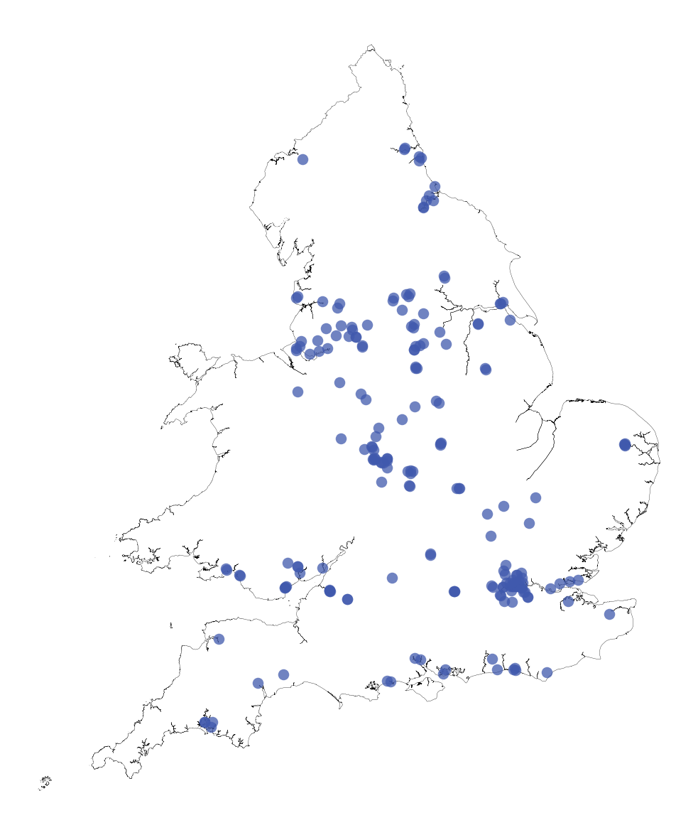
(a) 202 Urban Stations

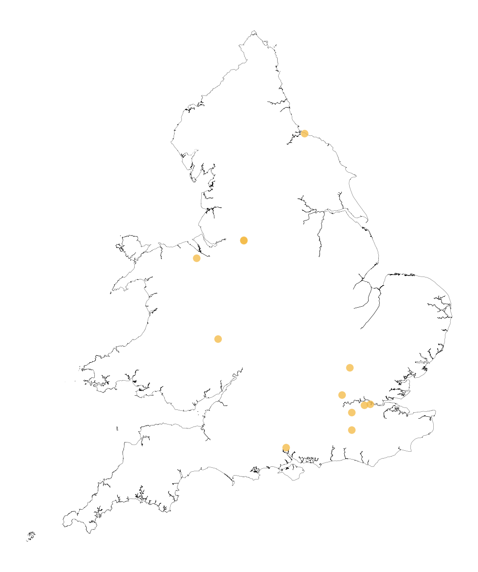
(b) 12 Suburban Stations

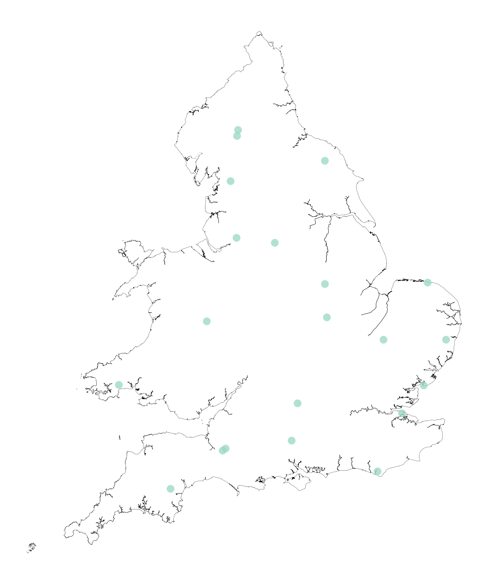
(c) 21 Rural Stations

Figure 1: Spatial distribution and classification of monitoring stations within England and Wales. The Automatic Urban and Rural Network (AURN) stations are divided into 3 classes: urban (202), suburban (12), and rural (21). Note the inequality of station numbers; most of the stations are in urban settings. The AURN has 274 stations total out of which 235 are in England and Wales

Given the gaps that exist in ground monitoring, model estimates for air pollution can supplement the ground observation network to ensure compliance with policy targets across the whole of the UK (Department of Environment, Food and Rural Affairs, 2019a, ). The UK’s air pollution datasets are augmented with outputs from the UK DEFRA Modelling of Ambient Air Quality (MAAQ) model, which like other aforementioned models suffer from shortcomings such as lack of transparency; we do not actually know the details of how this model works.

The goal of this work is threefold: (i) we want to estimate pollution concentrations based on datasets that are already available in most countries (road infrastructure properties); (ii) we aim to achieve the same or better results of current models using open source input data while also making the model itself open source, ensuring no barrier to implementing the approach based on cost alongside making the approach accessible; (iii) the process is made as streamlined as possible using minimal data to inform data acquisition for policymakers constrained by a lack of data availability, which is becoming an increasing divide between countries (Karlsson,, 2002).

The amount of data collected around the world and the fact that information about a phenomenon can be embedded in datasets collected for other purposes, mean that lack of data to be used in air pollution models may not necessarily be an excuse for not having a model. This work shows that we can effectively use secondary datasets containing information about the phenomenon we want to model; this can be important in locations where data is collected by institutions such as non-profits, foundations, the United Nations, etc. but no curated pollution datasets exist.

We chose the UK (England and Wales) as the study area to build a proof of concept model, as its air pollution monitoring data are open source and freely available. However, we see no reason for not being able to use a similar approach in other locations around the world, as long as we have similar data used here.

When dealing with spatial data, we often have to choose the aggregation level for the model. We chose Middle Layer Super Output Areas (MSOA) as the districts under which we would aggregate the road and air pollution data. The three district designs considered can be seen in Section LABEL:S-sec:MAUP. The OS National Grid district design was ruled out because many districts had no roads, which created districts where we could not create a feature vector. A feature vector is an ordered list of features about an observed phenomenon. Each feature describes a measurable property of the observed phenomena, in this case, the road network within a given district. A corresponding target vector is then created, in which the goal is for the model to learn the relationship between the corresponding features and targets. This study’s target vector is related to observed ambient air pollution concentrations within a district. The Local Authority District (LAD) design was a viable option but had very inconsistent geographical sizes for the different districts across the study area, ranging from 2.8km² area in the City of London LAD to 26,159.6km² area in the Highland LAD, alongside only 381 districts. The MSOA design offered a higher number of districts (at 7,201) while also providing a measure of population density with the population for each MSOA readily available; the population density then allowed for an estimation of how urbanised an area was in a continuous spectrum from least to most urbanised.

3 Data and Methods

In this work, we used OpenStreetMaps (OSM) data from 2014-2019. We selected 2014-2017 for training the models, 2018 for the test set, and 2019 for data exploration and parameter searching. Data prior to 2014 is quite sparse and post 2019 was avoided in this first instance because of the COVID-19 pandemic, which have resulted in changes in the way people behave spatially (Santana et al.,, 2022) and also because the COVID-19 pandemic had significant implications on air pollution across the world (Brown et al.,, 2021).

The OpenAir package (Carslaw and Ropkins,, 2012) provides access to data from the UK Automatic Urban and Rural Network (AURN) (Stevenson et al.,, 2009) with measurements taken every 15 minutes. Data starts from early 1973. Our study focused on 12 pollutants: Carbon Monoxide (CO), Nitrogen Oxide (NO), Nitrogen Dioxide (NO${}_{\text{2}}$) Nitrogen Oxides (NO_x), Particles < 10$\mu$m (PM₁₀), Particles < 2.5$\mu$m (PM₂₅), Non-volatile PM₁₀ (NV₁₀), Non-volatile PM₂₅ (NV₂₅), Volatile PM₁₀ (V₁₀), Volatile PM₂₅ (V₂₅), Ozone (O${}_{\text{3}}$), and Sulphur Dioxide (SO${}_{\text{2}}$). The number of active AURN stations per pollutant by year is shown in Figure LABEL:S-fig:ActiveAURNStations

Inverse Distance Weighting (IDW) Interpolation (Shepard,, 1968) was used to achieve full spatial coverage of the study area from the AURN ground observations by creating a raster from which air pollution values at specific locations could be sampled; IDW interpolation uses a power parameter to determine the effect of neighbouring sample points on a location’s value which can be tuned for specific air pollutants that are more or less susceptible to neighbouring pollution. We experimented with a range of possible values from 0 to 3.5 to determine the power parameter value for each pollutant, with the value that minimised the root-mean-square error (RMSE) (Daintith,, 2009) from leave-one-out-validation process used; Figure LABEL:S-fig:RMSEInterpolationPowerScatterPlots shows the plots for various power parameter values which were used for the choice of the power parameter. Figure LABEL:S-fig:InterpolationIDWSurfaces shows the raster produced by the IDW process with the best performing power parameter for each of the 12 pollutants.

We compared the resulting raster to the UK Government DEFRA air pollution model output for the same year, 2019 (Department of Environment, Food and Rural Affairs, 2019b, ), to verify the suitability of using interpolation to create a raster from ground observations. The dataset from the DEFRA model gives point estimates with a 1km resolution. We sampled the raster produced at the exact location of the 1km point, which we then aggregated to the district level, giving a value for the pollution in a given area.

We conducted a Pearson correlation coefficient (Benesty et al.,, 2009) analysis was calculated between the DEFRA and interpolated output shown for various road length per district to ensure that the relationship between datasets was similar. We achieved a correlation value of 0.95 and 0.94 indicating that the datasets describe the same phenomena and the IDW process is able to replicate the point sample annual observation on a complete spatial scale. The spearman rank-order correlation coefficient (Spearman,, 1961) was also calculated between the DEFRA and interpolated districts to ensure they had a similar ordering of the most / least polluted districts. The correlation value was high at 0.98 indicating that there is also agreement between the two datasets as to which districts are the most and least polluted across the study area. Figure 2 shows the pearson correlation plot between the DEFRA and interpolated output and the road length within a given district.

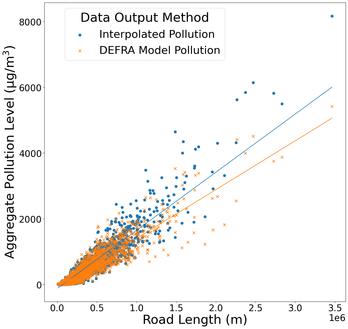
Figure 2: AURN ground observations interpolation vs. DEFRA air pollution model. Comparison between the two approaches. The blue points and line of the best fit depict the relationship between total air pollution in an MSOA (acquired via interpolating ground observations). In contrast, the orange points and line of the best fit represent air pollution data acquired via the UK DEFRA Ambient Air Quality Contract Model. The chart shows the two measurements of pollution, ordered by road length (x-asis). A similar relationship between the two lines of best fit indicates that the methods for generating the air pollution data are similar

OpenStreetMaps is an open-source collaborative project that contains road data for most parts of the world, and it is quite comprehensive for the UK (OpenStreetMap contributors,, 2021). The method used to create historical road infrastructure datasets was to use the OpenStreetMaps history files (.osh.pbf) to revert an OpenStreetMaps file (.osm.pbf) to its state at a given point in time. We could then use the historical OpenStreetMaps file to extract the network’s structural properties at that time, such as the total road length per district.

The feature vector within our study is based on the length of the road network within a given area, determined by summing the length of the roads within the district under the WGS 84 / World Mercator EPSG: 3395 coordinate reference system (CRS), giving the length of the line segments of roads in meters. This process is then repeated for each of the MSOA districts. Each MSOA district then gives one element to the final feature vector for a given time.

The target vector is created by summing point estimates across a uniform point grid with 250m intervals. We chose the 250m interval to ensure that every MSOA had a point estimate. Details of the uniform point grid used can be seen in Table LABEL:S-tab:Table_2_Target_Vector_Example, alongside a visualisation for a single MSOA in Figure LABEL:S-fig:ToyExampleOfRasterSampleWithUniformPointGrid.

We observed a positive linear correlation between the total road network length and the annual aggregate air pollution within a district. This correlation is shown in Figure 3 for the pollutant PM2.5 in 2019. This observation led us to use a linear model to predict the annual level of air pollution. The Pearson correlation coefficient between the aggregated interpolation pollution and road length was 0.943.

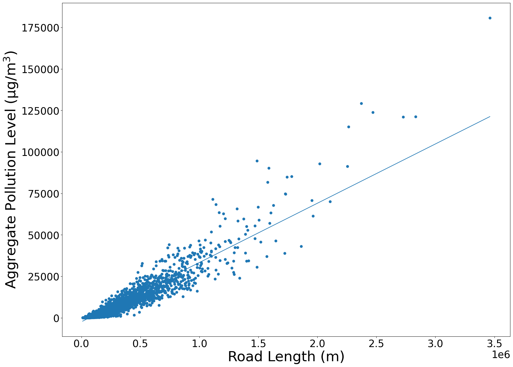
Figure 3: MSOA district road network total length vs aggregate PM2.5 pollution in 2019. Line of best fit for a set of points depicting the relationship between the aggregate PM2.5 pollution within an MSOA and the total road length within the corresponding MSOA. The linear relationship led to our decision to use a linear regression model

4 Methodology

4.1 Models

We used three variations of the model using different feature vectors. Example feature vectors and predicted pollution values for the models can be seen in Section LABEL:S-sec:modelDetails.

The first developed model aimed to predict a district’s pollution from the total road network length; a simple linear regression (Freedman,, 2009) was used. The results from this model can be seen in Table 1, detailing the mean absolute error, mean squared error, and the R² (coefficient of determination) (Draper and Smith,, 1998). This table should be seen in conjunction to the other tables described later to allow a fair comparison between the models. An example feature vector for the length model can be seen in Table LABEL:S-tab:Table_4_Curated_Example_Length_Feature_Vector, with predictions made by the model shown in Table LABEL:S-tab:Lenght_Model_Example_Outputs. In relation to Figure 4 the model only considers the total length of the blue road network.

Pollutant Name	Mean Absolute Error (µg/m3)	Mean Squared Error (µg/m3)	$R^{2}$ Coefficient of Determination
CO	$57.808$	$11,254.374$	$0.544$
NO	$3596.192$	$42,036,395.288$	$0.711$
NO2	$4748.005$	$71,646,196.869$	$0.819$
NOx	$10,277.881$	$337,089,243.351$	$0.773$
NV10	$2458.049$	$19,646,741.387$	$0.861$
NV25	$1484.307$	$7,014,357.411$	$0.842$
O3	$7956.092$	$221,380,110.422$	$0.871$
PM10	$3005.557$	$29,519,093.175$	$0.859$
PM25	$1942.964$	$12,019,157.647$	$0.842$
SO2	$546.223$	$1,006,964.606$	$0.533$
V10	$559.122$	$1,027,117.426$	$0.858$
V25	$477.524$	$733,041.363$	$0.86$

Table 1: Results from the length feature vector model using all road types. The results show that model performance achieves a high of 0.87 in $R^{2}$ score across the 12 pollutants. Of note is that CO and SO₂ have a lower score of around 0.535. As shown in Figure LABEL:S-fig:RMSEInterpolationPowerScatterPlots the interpolation process was unable to estimate a power parameter for the sample locations for CO, SO₂, V₁₀, indicating that there are not enough stations within the UK to pick up the variability over the distances separating the stations at the annual temporal level. However, V₁₀ achieved a 0.86 R2 score. The reason for this discrepancy between the three pollutants is the change in air pollution between the training (2014-2017) and test year (2018). For the V₁₀interpolated raster, a change of concentrations from 3.03 (µg/m³) in 2017 to 3.16 (µg/m³) in 2018 (4.3% increase) was observed. The change in V₁₀ was considerably smaller than in CO, decreasing from 0.22 (µg/m³) in 2017 to 0.18 (µg/m³) in 2018 (18.2% decrease). Similarly, SO₂ decreased from 1.99 (µg/m³) in 2017 to 1.73 (µg/m³) in 2018 (13.1% decrease). The Mean Absolute Error is included to give a context of the model performance between pollutants with considerably different maximum values, as seen in Figure LABEL:S-fig:RMSEInterpolationPowerScatterPlots. The Mean Squared Error is also included to highlight the model’s performance concerning the more extreme values seen within the dataset, which are experienced due to the varying geographical sizes of the districts being estimated.

The second variation of the model splits the road network into the different types of highways (roads) detailed in the OpenStreetMaps database (OpenStreetMap contributors,, 2021), and created a length element per road type in the feature vector. In relation to Figure 4 the feature vector still only considers the blue road network but now creates a separate feature for each road type, such as the solid black lines denoting the residential roads within the blue road network. An example feature vector for the composition model can be seen in Table LABEL:S-tab:Table_7_Curated_Example_Highway_Composition_Feature_Vector, with predictions made by the model shown in Table LABEL:S-tab:Curated_Highway_Composition_Model_Results. A multiple linear regression (Freedman,, 2009) implemented this model. The results from this model can be seen in Table 2, detailing the mean absolute error, mean squared error and the R² (coefficient of determination) (Draper and Smith,, 1998). When contrasting this with Table 1 which uses the total length of roads, it becomes clear that this model in which lengths are separated per type of road performs better.

Pollutant Name	Mean Absolute Error (µg/m3)	Mean Squared Error (µg/m3)	$R^{2}$ Coefficient of Determination
CO	$37.885$	$7105.308$	$0.712$
NO	$2275.254$	$24,531,005.517$	$0.832$
NO2	$2787.602$	$33,815,646.291$	$0.915$
NOx	$6244.618$	$176,639,841.556$	$0.881$
NV10	$1358.646$	$7,912,333.282$	$0.944$
NV25	$840.539$	$2,965,264.271$	$0.933$
O3	$4429.423$	$90,029,016.993$	$0.948$
PM10	$1672.108$	$12,032,403.918$	$0.942$
PM25	$1104.896$	$5,172,685.475$	$0.932$
SO2	$357.653$	$632,527.654$	$0.707$
V10	$313.205$	$423,503.083$	$0.941$
V25	$265.856$	$297,593.321$	$0.943$

Table 2: Results from the composition feature vector model using all road types. The $R^{2}$ for all air pollutants has improved over the length model detailed in Table 1, alongside reducing both the Mean Absolute Error and Mean Squared Error, indicating an improved model framework for estimating air pollutants, with the same relative performance between air pollutants. Note that this model is also based on road lengths, but the lengths here are not the total but based on road type.

The third model created was a spatial variant of the second model, using the same multiple linear regression technique as the composition model. We created the spatial model to capture whether the district was in the centre of an urbanised zone, on the outskirts or wholly removed, as the primary sources of a district’s air pollution might be outside the district’s boundaries. The feature vector for the spatial model comprised the same features as the composition model; however, the process conducted for the blue road network within Figure 4 was repeated for the yellow road network, providing a total length of the adjacent district’s road networks, thereby doubling the number of features present with the feature vector over the composition model, as seen in Table LABEL:S-tab:Table_10_Curated_Example_Spatial_Feature_Vector. Predictions made by the spatial model are shown in Table LABEL:S-tab:Table_11_Curated_Spatial_Predicition. The use of an additional set of elements that give values for the sum of the road network length by road type in adjacent MSOAs to the estimated district has the effect of something akin to a network in which the neighbours influence the values of the current location, causing the values used in the composition model feature vector to be more contextualised. The results from this model can be seen in Table 3, detailing the mean absolute error, mean squared error and the R² (coefficient of determination) (Draper and Smith,, 1998).

While the improvements in the $R^{2}$ score are minimal, there is no overhead cost in creating the additional features for the vector as data collection concerning the roads has already taken place. Similar computational costs between the models also arguably make the time investment worthwhile, as there are minimal barriers to implementing the spatial variant of the composition model.

Overall the three different variations of the model help alleviate a specific situation that could be encountered and have varying benefits. The length model has the benefit of being conceptually simple, allowing multiple datasets to be integrated due to the universal property of road length between datasets. The composition model offers improvements over the length model but restricts the datasets that can be used where the classification schema is consistent across the study period. Finally, the spatial model offers some further performance improvements but requires considerably more data than the composition model, alongside adding further complexity to the model itself.

Pollutant Name	Mean Absolute Error (µg/m3)	Mean Squared Error (µg/m3)	$R^{2}$ Coefficient of Determination
CO	$38.35$	$6698.946$	$0.729$
NO	$2320.79$	$23,905,675.199$	$0.836$
NO2	$2845.108$	$31,823,322.218$	$0.92$
NOx	$6363.865$	$169,035,020.271$	$0.886$
NV10	$1398.695$	$7,467,525.593$	$0.947$
NV25	$863.295$	$2,779,375.839$	$0.937$
O3	$4582.988$	$86,357,497.527$	$0.95$
PM10	$1721.591$	$11,341,938.593$	$0.946$
PM25	$1133.152$	$4,837,131.307$	$0.936$
SO2	$361.93$	$592,487.886$	$0.725$
V10	$323.345$	$399,460.291$	$0.945$
V25	$273.781$	$280,215.091$	$0.946$

Table 3: Results from the spatial composition feature vector model using all road types. The $R^{2}$ has improved for some of the pollutants included within the study over the composition model detailed in Table 2 other than NO${}_{\text{2}}$, O${}_{\text{3}}$, however not all the metrics have improved in the same manner as the transition from the length to composition model, for example with the Mean Absolute Error and Mean Squared Error increasing, potentially indicating a less robust model framework for estimating air pollutants that requires additional data over the other model’s details in Table 1 and Table 2.

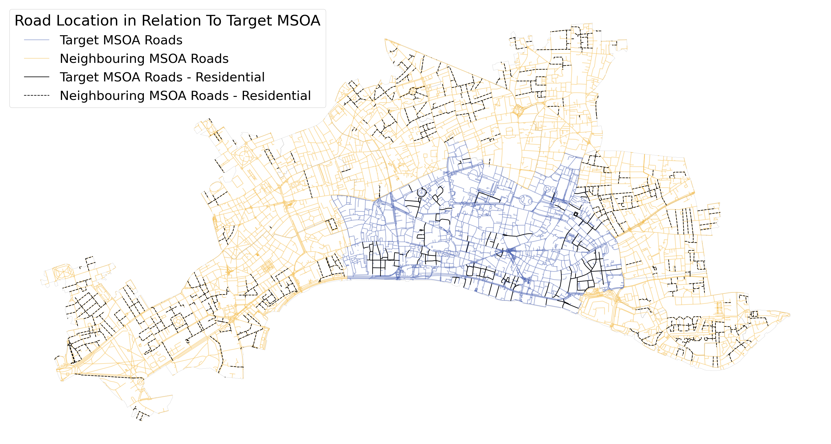
Figure 4: Road network structure within MSOA City of London 001 (blue) and surrounding MSOAs (yellow). The solid black line represents the residential roads within MSOA City of London 001 and the dashed black line the residential roads within the neighbouring MSOAs. The road network will contribute differently to the feature vector values depending on the framework used. In the case of the length model, the simple overall length of the road network is used, which for MSOA City of London 001 is 223,092m (in meters), visualised with the blue and black solid lines. In the case of the composition model, each road type contributes to a different single feature vector element, with the black solid residential road contributing a single element of the feature vector with the value 23,235m. The spatial variant of the model takes into account the total road length for different road types in adjacent MSOAs alongside the considerations of the composition model, meaning the total for the dashed black line compromises a single element of the feature vector used, in this case, 82,500m

4.2 Feature Selection

The OpenStreetMaps dataset is exceptionally comprehensive with regards to road information. The feature vector in the previously described models included all road types within the OpenStreetMaps dataset. There are 99 different road types but some are misclassified (shown in tables in Section LABEL:S-sec:featureSelectionDetails). This section describes the work conducted to reduce the input dataset’s size to only what was needed to achieve the goal of estimating air pollution within a district.

Given the number of variables (road types) that exist in the OpenStreetMaps dataset, we relied on information theory Shannon, (1948) and in particular mutual information between the road types and the different air pollutants to determine which road types have the highest relation with each air pollutant. As mentioned above, the initial number of road types in the dataset was 99. Removing road types that had no relevance to the air pollutants being studied, represented by a mutual information summation value of 0, kept 88 road types. The types removed were mostly misclassifications by a user inputting a road type, such as "fence" or "residential;footway". Our next step was incrementing the threshold for removal for a road types summation value and comparing the resulting model’s performance by its $R^{2}$ score. Figure 5(a) shows a plot of the resulting $R^{2}$ score for both the length and composition models against differing numbers of road types subset by the value of the threshold for inclusion of the mutual information summation. Table LABEL:S-tab:Every5thMutualInformationPerPollutant shows mutual information values for the pollutants across a range of road types, and Table LABEL:S-tab:R2ValuesAll99HighwaysFeatureSelection shows the model’s performance with reduced input datasets.

(a) Starting with all 99 road types.

(b) 25 road types relevant to all air pollutants.

Figure 5: Model performance vs $R^{2}$ score, with road type inclusion based upon road type mutual information with air pollution. Shown is the performance of the length and composition model when removing certain roads from being included as part of the feature vector. Inclusion in the feature vector depends on the sum of mutual information of the road type with pollutants considered in the study. A threshold is incremented to remove the road types with less mutual information than others. The requirement for a non-zero mutual information sum removes 11 road types with no relation to pollution, such as the OpenStreetMaps classification of turning circles, leaving 88 road types. Many road types have a minimal sum for mutual information, so incrementing the threshold to 0.1 removes 65 road types, with classifications such as living street removed. This process is then repeated until a single road type remains, in this case, the track road classification, which can be seen at which point the length and composition model reduces to the same model. Figure 5(b) details the same experiment detailed in Figure 5(a) however only road types that have a non zero value for mutual information with all pollutants were considered, leaving 25 road types, removing road types such as lane that only have a non zero mutual information values with SO${}_{\text{2}}$

We then repeated the experiments; however, we included only road types relevant to all 12 pollutants in the test. 25 out of 99 pollutants had relevance to all 12 pollutants to be estimated; relevance is measured by ensuring that the road type had non-zero mutual information for all 12 pollutants. The results of this experiment are shown Figure 5(b). Table LABEL:S-tab:Table_14_R2_Values_Highway_Types_22_relevant_highway_types shows the results from the previous three models with road types with zero mutual information with at least one of the pollutants.

In Figure 5, the best model uses two road types, track and unclassified, to predict the pollution within a district, seen distinctly with an increase in the $R^{2}$ score for the length model to 0.83, up from 0.78. We can see that some road types cause the length model to perform worse, but even when the result improves, it never performs as well as the composition model. Eventually, with only one road type remaining, the length and composition model are reduced to the same linear regression model, producing an $R^{2}$ score of 0.65.

We performed pairwise mutual information between the road types to further reduce the dataset. The goal was to determine the road network types that contained the most information about other road types within the dataset. The road types we performed the mutual information on were the 25 road types with some mutual information with every pollutant covered in the study.

Figure 6 shows a heatmap of the mutual information values between the 25 road types. The values in the heatmap have been normalised row-wise. In the heatmap, there are 625 data points. 457 points have a value of mutual information greater than zero. Some data points have a value of 0 for mutual information; for example, living street and raceway have zero pairwise mutual information.

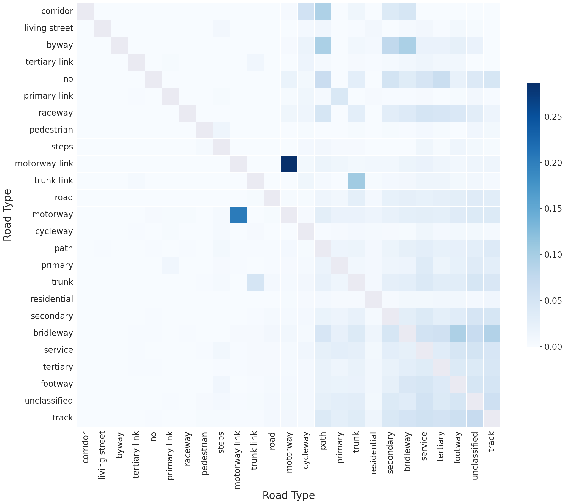
Figure 6: Mutual information between road types. The heatmap shows the mutual information between all 25 road types with a non-zero mutual information value with all the pollutants in the study. The heatmap values are normalised by row with the diagonal removed (which has value 1), allowing for an understanding of which road type has the highest mutual information to the other road types in the dataset. Motorway link has the highest mutual information with the motorway road type. While the motorway type has strong mutual information with the motorway link type, there are also strong mutual information scores with other road types, such as track and path. This difference in the strength of mutual information indicates that the motorway link dataset contains information mainly about the motorway road type, but the motorway dataset contains information about motorway link and other road types such as track, path etc., giving it a more desirable use in retaining information about all datasets (values are normalized by row and the diagonal removed)

The heatmap was modelled as a network of the 25 road types to determine the road types that contain the most mutual information about other road types, as shown in Figure LABEL:S-fig:NetorkModelMutualInformation. Each node in the network represents a road type, and the edge weight between the two nodes is the mutual information between the two road types. The degree of each node is equal to the sum of the weights of the edges adjacent to the given node, giving a value for the amount of mutual information a given road type contains about other road types in the network.

The node with the highest degree was chosen for inclusion in the model feature vector and then removed from the network as the mutual information of the edges no longer needed to be included in the dataset. This process was repeated, with the next highest node based on degree weight chosen, until no nodes remained. The results of this process on the network representation can be seen in Figure LABEL:S-fig:NetworkModelRemoveTimesteps.

The test results in Figure 7 show that a model underpinned by the “track” and “unclassified road” road type produce a model with an $R^{2}$ score of 0.83 while only making use of 25.9% of the total road network length in the study area. Indicating that these two types of roads are sufficient to provide a good estimation of air pollution.

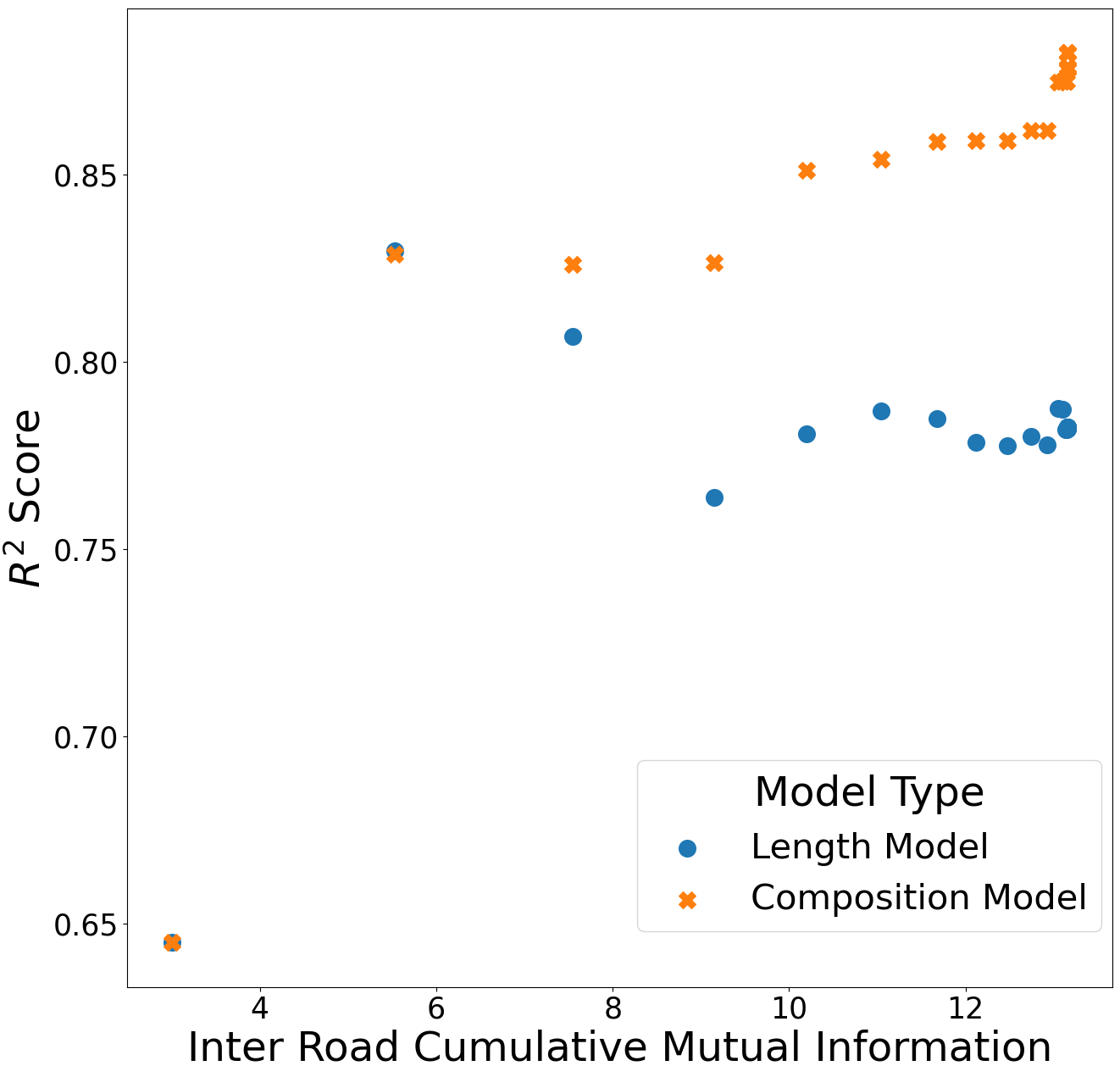
Figure 7: Total inter road cumulative mutual information in input feature vector vs $R^{2}$ score. Shown is the performance of the length and composition model when removing road types from being included as part of the feature vector based on the road type’s mutual information with other roads, aiming to reduce the data required while maintaining performance by including road types containing information about other road types. A single road type was removed at each step, with the x-axis detailing the total remaining mutual information about other road types within the datasets used for the feature vector. Eventually, the model reduces into the same model when only a single road type remains. The performance improvement of the length model as some road types are removed indicates that some of the datasets included are noisy and affect model performance; this issue is not present with the composition model that can differentiate different road types, seen with a gradual reduction in model performance. The full experiment results can be seen in Table LABEL:S-tab:Inter_road_mutual_information_tests

4.3 Missing Districts Tests

We also conducted experiments to explore whether some districts within the study area could be used for training, having the remaining districts estimated from the model created. The idea was to reduce the input dataset further by removing similar districts from the training set, retaining only a subset of urban, suburban or rural districts. The population density was used as a proxy metric for how urbanised a district is, with example districts shown in Table LABEL:S-tab:Table_17_Population_Density. The goal was to understand the minimal number of roads that need to be measured across different districts to predict pollution across all districts accurately. We did not include the spatial variant in these tests, as it would require additional data acquisition over the minimal amount of measuring needed for just the district itself. We used the data from 2018 for the tests. For a set of 16 random states, different MSOAs were randomly sampled from the 7201 total MSOA districts. When selecting the additional districts to be included in the test, we ensured that the districts used in the previous iterations were still present. For example, the districts used in one random state in the 100 training size set were also used in the 500 training size set, as visualised in Figure LABEL:S-fig:InterYearExperimentTrainingSetsVisualisation.

Table LABEL:S-tab:Table_18_Inter_year_tests shows the results for the mean $R^{2}$ score for both the length and the composition model for reducing training set size across 16 random state tests. We chose to explore test set sizes ranging from 100 MSOAs to 7200 MSOAs, with the training set being made up of the remaining MSOAs, for example, 100 MSOAs in the test set and 7101 MSOAs in the training set.

Figure 8 shows the scatter plots for the data detailed in Table LABEL:S-tab:Table_18_Inter_year_tests. The random tests show that the length model is more robust than the composition model, indicating that the composition of the road network between different districts can vary greatly, resulting in poor performance in some random training sets. The length model maintains performance as the training size is reduced from the initial 7101 MSOAs to 26 MSOAs, with an $R^{2}$ score of 0.85. After this, the performance of the model begins to decrease. Across a range of different random states, around 26 MSOAs need to be used to train the model to successfully predict all MSOAs pollution, representing 0.36% of the total number of MSOAs.

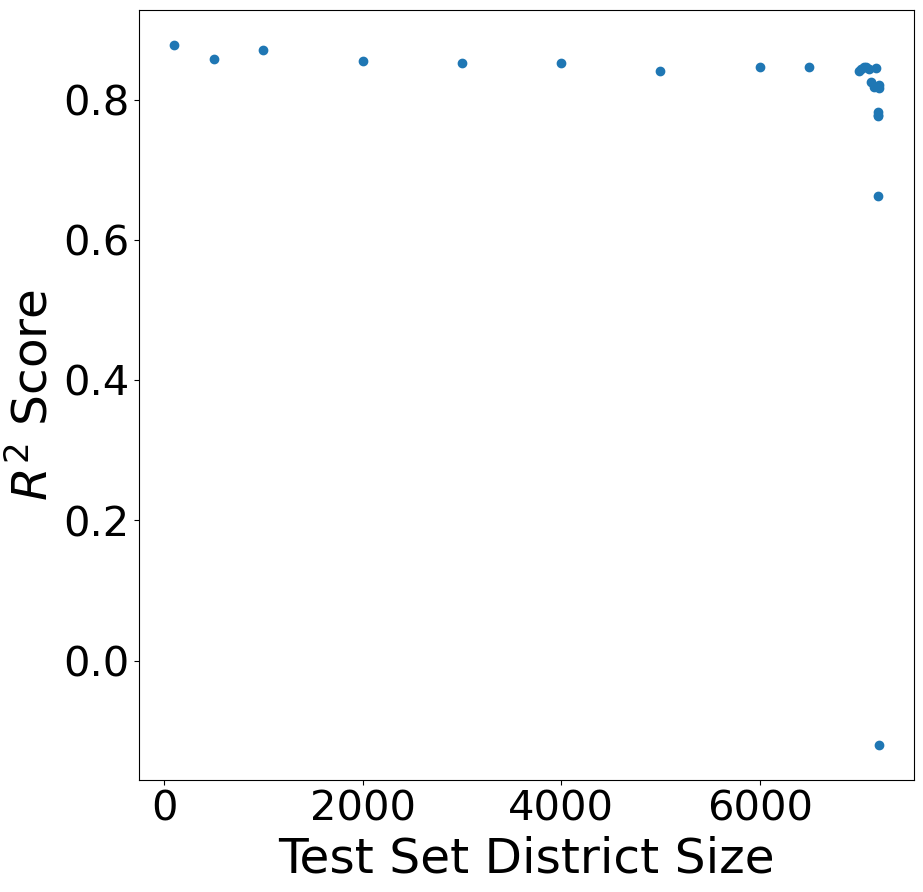
(a) Length Model

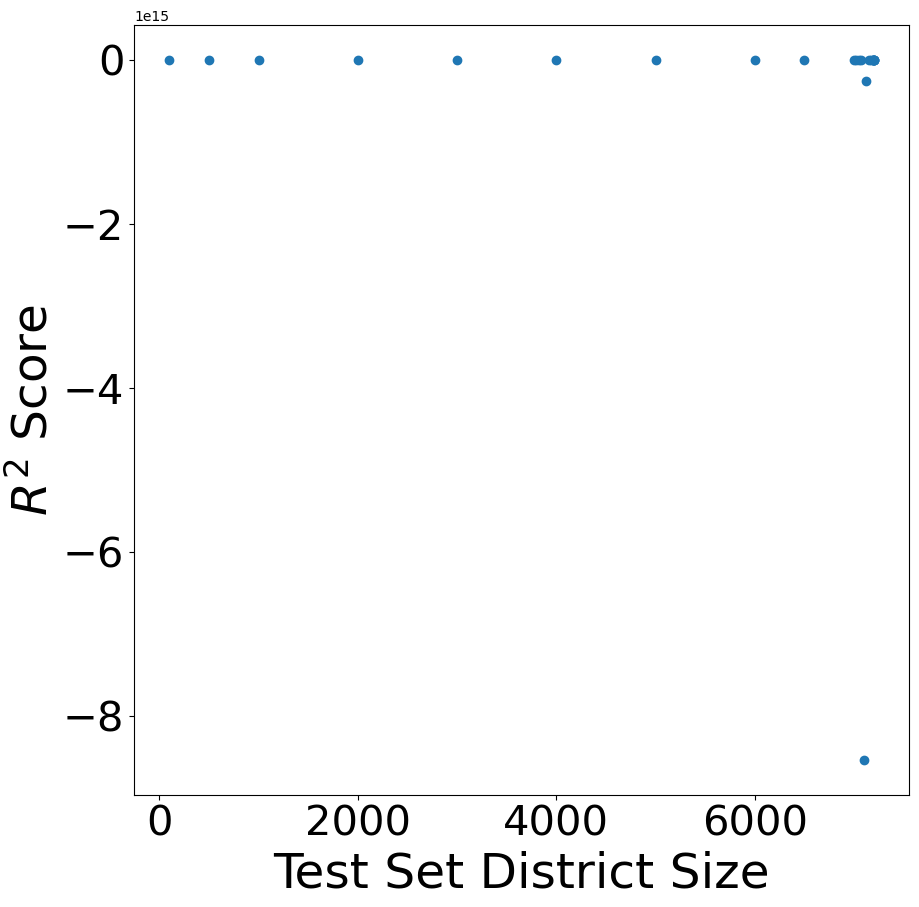
(b) Composition Model

Figure 8: Test set size districts vs $R^{2}$ score. Shown is the performance of the length and composition model as the input districts for the training set are reduced from 7101 to 1. Of note is the difference in the scale of the y-axis between the figures. As the test set size increases (and so the training set size decreases), the performance of both models remains stable until the test set comprises 7,175 out of 7,201 (0.36%) districts. At that point, both models begin to reduce in performance. The length model maintains its performance at around 0.8 $R^{2}$ score for longer, with the composition model degrading to an average $R^{2}$ score of 0.65. When the test set size is 7,200, meaning only a single district is used as the training set, both models break down worse than just estimating the average air pollution value; however, the composition performs significantly worse than the length model. Thereby indicating that while the composition model performs better than the length model initially, it does require more input data to perform well

As seen in Figure 8, the $R^{2}$ score for the length model averaged 0.83, providing a baseline performance for the next experiment. We trained a set of models with 1500 districts with similar population densities to explore the effect of changing population density distribution in the training set on model performance. Starting from the least urbanised MSOAs, to the most urbanised MSOAs, with increments of 125, a model was trained and the $R^{2}$ score computed. The results from this experiment are shown in Figure 9, where the average $R^{2}$ score across the 46 tests was 0.83. The $R^{2}$ score remained similar to the expected 0.83 from the random tests as the training set changed from least to most urbanised. Thus, pointing toward the idea that the $R^{2}$ score of the length model is not related to the population density distribution of the MSOAs included in the subset of training districts.

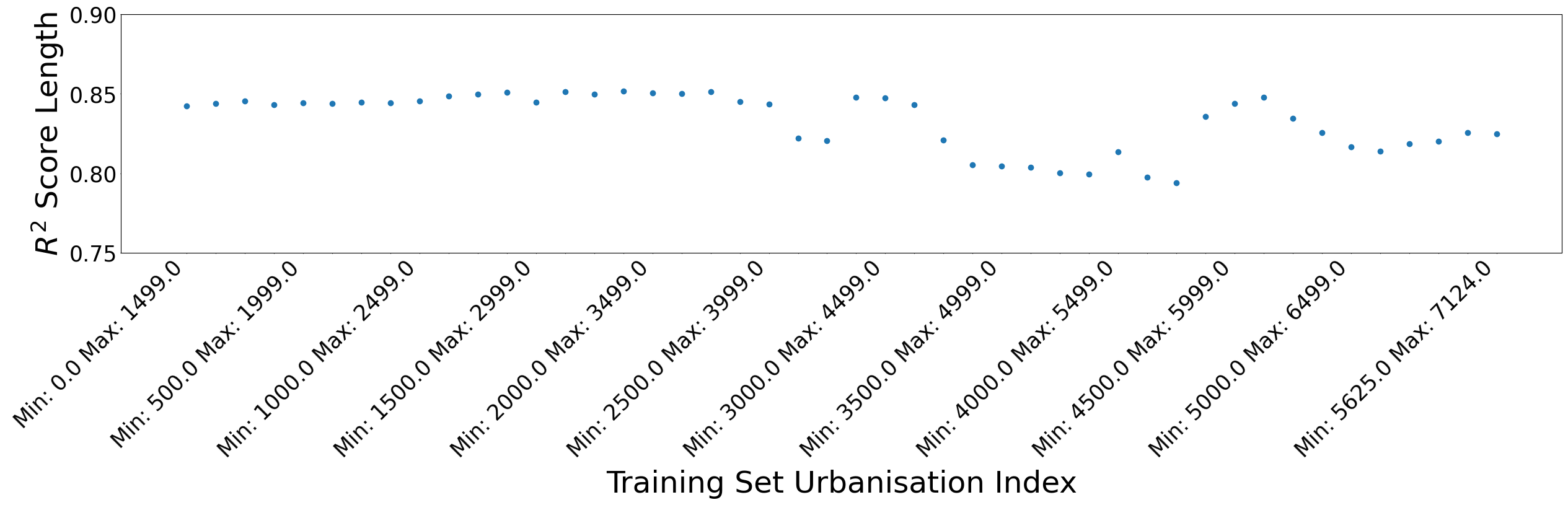
Figure 9: Test sizes vs $R^{2}$ score for length model for changing population density within the training set. Shown is the length model’s performance across a range of training sets chosen based on the MSOAs population density. The population density for an MSOA is used as a proxy for how urbanised an MSOA is; the higher the population density, the more urbanised an MSOA is. 1,500 MSOAs were chosen to be part of each training set, with the variation being in the average population density of the training set MSOAs. The first point (Min 0 Max 1,499) is where the least urbanised MSOAs are the training set. The last point (Min 5,625 Max 7,124) is where the most urbanised MSOAs are the training set. The consistent performance of the length model as the average urbanisation of the training set MSOAs increases indicates how urbanised an MSOA does not affect the model performance. Table LABEL:S-tab:trainingSetSizePopulationDensity shows the full experiment results

5 Use Cases

From the tests conducted as part of this work, the critical road types to predict the pollution in an area are the “minor roads”; the road types “track” and “unclassified” within the OpenStreetMaps classification schema. Not only do the road types “track” and “unclassified” have the most mutual information about the 12 pollutants analysed within this study, with a normalised summation value of 12 and 10.12 respectively, but they also contain the most mutual information about the other road types with a total value of 2.97 and 3.00 respectively. The “track” and “unclassified” road type input data produce a model with an $R^{2}$ score of 0.83 for both the Length and Composition model. The model then degrades to an $R^{2}$ score of 0.65 when only the “track” road type is included, where the length and composition model is the same. While the $R^{2}$ score of the complete composition model, with all 25 road types, improves to 0.89 compared to the length models $R^{2}$ score of 0.78, an argument is that the increased amount of data needed to attain the increase of 0.11 on the $R^{2}$ is not worthwhile. The entire length of the road network within the MSOA boundaries in 2018 is 1,140,835,548m, out of which 295,948,514m, represents the “track” and “unclassified” road network, representing a 74.1% reduction in input data for minimal performance loss. However, it is also vital to consider the context in which the model is intended for use. The model was never designed to accurately predict the pollution in an area to a specific value, but rather to give an idea of where it is most polluted within an area to help identify areas for intervention. Within this context, the loss of 0.11 $R^{2}$ score is meaningless in the model’s practical use.

The missing districts tests have clear implications on the approach of deploying monitoring stations to create a target vector. The experiments show that a distribution of urban, suburban and rural districts across the training set is unnecessary. In the UK case, only about 0.36% of districts, or 26/7201 districts, were required to accurately predict pollution across all districts at the annual level. Using the model proposed would allow policymakers to have full spatial coverage of air pollution while only deploying monitoring stations in 0.36% of districts, representing significant monetary savings over deploying a comprehensive air pollution monitoring network like the UK’s AURN.

The findings of this study show that a linear regression model underpinned by a single structural property, length, of the track and unclassified road network within 0.36% of districts within England and Wales was enough data to identify an ordering for which districts are the most polluted. Furthermore, the model discussed presents a low-cost method of achieving similar results to more expensive models such as the one currently used by DEFRA. The model has apparent practical uses for policymakers that want to pursue clean air initiatives but lack the capital to invest in comprehensive dedicated monitoring networks.

6 Discussion

In this work, we presented a solution for the estimation of annual air pollution using a dataset related to the structure of roads, we have focused on a model based on length of roads and also on a composition model which consider other factors associated to road classifications.

Our contributions can be split into 3 categories. (1) We have shown that one can get to good annual estimations on a very low budget. This contrasts with current approaches in the UK which costs millions of pounds (£). Making an approach that is cheaper and accessible to multiple stakeholders is more inclusive, allowing society to use the estimations in secondary applications (health exposure, traffic, city planning, etc.) (2) Our model is quite transparent, and the characteristics used as well as the estimator based on simple regressions is quite explainable. This leads to a better reusability and generality of the approach. (3) In a more general sense, we believe this work has an impact on showing that in data science and in particular, environmental data science, lack of data about a particular phenomenon can be overcome by using the information embedded in other datasets which may not have been collected with that intent. This happens due to mutual information, in which aspects of one phenomenon may be present in other pieces of information.

While the use of road length is inferior at estimating air pollution to approaches that use dynamic data, the method presented has the benefit of a nominal implementation cost due to the data’s open source nature, minimal training computation, and accessible model design. The missing districts experiments give a framework for using a minimal amount of monitoring stations across an area, in the case of the UK, 0.36% of MSOAs, and use the model presented to fill in missing districts, producing a full spatial map of air pollution at the annual temporal level. The full spatial map ensures that all districts, urban, suburban and rural alike, have an estimate for ambient air pollution, helping to address inequality related to a current focus on urban areas with monitoring station placement.

While the composition model surpassed the length model in performance, there is a trade-off in operationalising the composition model over the length model due to the data used. The length model has the benefit of using a universal structural property of roads, its length, which is present across datasets such as OpenStreetMaps used in our study or other datasets concerning road networks such as Ordnance Survey Opens Roads . However, when using the composition model, there is an immediate limitation of being tied to a single dataset and the classification schema used for road types. For example, in the OS Opens Roads, there are only 6 classifications of roads, but as seen in Section 4.2, there were 99 different classifications in OpenStreetMaps. The road classification used also exposes the model to potential system shocks. One of them is the potential for OpenStreetMaps to change their classification schema, which could make it challenging to have a complete dataset that spanned multiple years. This issue is simple to solve with the length model, with the ability to combine datasets depending on their availability to extend the temporal coverage of the data used.

While the UK and many other global north countries can invest in comprehensive monitoring-station networks, this is not always the case for lower-income counties, particularly those in the global south. Data concerning annual air pollution globally would help to inform policymakers’ decisions and help to combat some of the 4.2 million death/year attributed to ambient air pollution (Public Health, Social and Environmental Determinants of Health Department,, 2018). The framework presented, paired with the global availability of road structural properties’ data through OpenStreetMaps, provides a basis for future work to design a global annual air pollution model from similar secondary datasets to those used in this study.

Future work could explore the possibility of using the same framework to estimate air pollution at a higher temporal level, such as the daily or hourly level. However, there are likely limits to the approach presented in this paper at a finer temporal level due to the static nature of road transport infrastructure. Future work would highlight the need to transition from data concerning the static elements of the road, such as its length, to more dynamic aspects of the road, such as the traffic counts of different types of vehicles. However, this data is more expensive to acquire and more invasive to privacy. Therefore, critical evaluations are needed whether the benefits derived from the model underpinned by more invasive dynamic data are worth the additional benefits of more accurate air pollution environmental intelligence.

Funding Statement

This research was supported by an EPSRC studentship awarded to LJ. Berrisford as part of the UKRI Centre for Doctoral Training in Environmental Intelligence.

Competing Interests

None.

Data Availability Statement

The road network data can be accessed via [https://download.geofabrik.de/europe/great-britain.html]. The boundaries for the MSOA used can be accessed via [https://statistics.ukdataservice.ac.uk/dataset/2011-census-geography-boundaries-middle-layer-super-output-areas-and-intermediate-zones].

Ethical Standards

The research meets all ethical guidelines, including adherence to the legal requirements of the study country.

Author Contributions

Conceptualization: L.B; R.M. Methodology: L.B; R.M; E.R. Data curation: L.B. Data visualisation: L.B. Writing original draft: L.B. Writing - Review and Editing L.B; E.R; R.M. Software L.B. All authors approved the final submitted draft.

References

- Agrawal, (2005) Agrawal, M. (2005). Effects of air pollution on agriculture: an issue of national concern. Natl Acad Sci Lett, 28(3/4):93–106.
- Aunan et al., (2019) Aunan, K., Hansen, M. H., Liu, Z., and Wang, S. (2019). The hidden hazard of household air pollution in rural china. Environmental Science & Policy, 93:27–33.
- Benesty et al., (2009) Benesty, J., Chen, J., Huang, Y., and Cohen, I. (2009). Pearson correlation coefficient. In Noise reduction in speech processing, pages 37–40. Springer.
- Brookes et al., (2021) Brookes, D. M., Stedman, J. R., Kent, A. J., Whiting, S. L., Rose, R. A., Williams, C. J., Pugsley, K. L., Wareham, J. V., and Pepler, A. (2021). Technical report on UK supplementary assessment under The Air Quality Directive (2008/50/EC), The Air Quality Framework Directive (96/62/EC) and Fourth Daughter Directive (2004/107/EC) for 2017. Technical report, Ricardo Energy and Enviroment.
- Brown et al., (2021) Brown, L., Barnes, J., and Hayes, E. (2021). Traffic-related air pollution reduction at UK schools during the Covid-19 lockdown. Science of The Total Environment, 780:146651.
- Carslaw and Ropkins, (2012) Carslaw, D. C. and Ropkins, K. (2012). openair — An R package for air quality data analysis. Environmental Modelling and Software, 27–28(0):52–61.
- Catalano et al., (2016) Catalano, M., Galatioto, F., Bell, M., Namdeo, A., and Bergantino, A. S. (2016). Improving the prediction of air pollution peak episodes generated by urban transport networks. Environmental science and policy, 60:69–83.
- Daintith, (2009) Daintith, J. (2009). A Dictionary of Physics (6 ed.) Root Mean Square Value (RMS value). Oxford University Press.
- DEFRA Network eTendering Portal, (2021) DEFRA Network eTendering Portal (2021). Modelling of ambient air quality contract. Technical report, Department for Environment, Food and Rural Affairs. https://www.find-tender.service.gov.uk/Notice/007858-2021?origin=SearchResults&p=1 "[Online; accessed August-2021]".
- Deng and Mendelsohn, (2021) Deng, H. and Mendelsohn, R. (2021). The effect of urbanization on air pollution damage. Journal of the Association of Environmental and Resource Economists, 8(5):955–973.
- (11) Department of Environment, Food and Rural Affairs (2019a). Air Pollution in the UK 2019 - Chapter 3 The Evidence Base. Technical report, Uk Government.
- (12) Department of Environment, Food and Rural Affairs (2019b). Modelled Background Pollution Data - PM25. https://uk-air.defra.gov.uk/data/pcm-data "[Online; accessed August-2021]".
- Draper and Smith, (1998) Draper, N. R. and Smith, H. (1998). Applied regression analysis, volume 326. John Wiley and Sons.
- Du et al., (2018) Du, W., Li, X., Chen, Y., and Shen, G. (2018). Household air pollution and personal exposure to air pollutants in rural china–a review. Environmental pollution, 237:625–638.
- Eustice and of Richmond Park, (2021) Eustice, G. and of Richmond Park, L. G. (2021). Environment Bill. https://bills.parliament.uk/bills/2593 "[Online; accessed August-2021]".
- Freedman, (2009) Freedman, D. A. (2009). Statistical models: theory and practice. cambridge university press.
- Gualtieri and Tartaglia, (1998) Gualtieri, G. and Tartaglia, M. (1998). Predicting urban traffic air pollution: a GIS framework. Transportation Research Part D: Transport and Environment, 3(5):329–336.
- Jim Stewart-Evans, (2019) Jim Stewart-Evans (2019). Review of interventions to improve outdoor air quality and public health. Technical report, Public Health England, Public Health England Wellington House 133-155 Waterloo Road London SE1 8UG. https://www.gov.uk/government/publications/improving-outdoor-air-quality-and-health-review-of-interventions "[Online; accessed September-2022]".
- Johnson, (2017) Johnson, C. A. (2017). Holding polluting countries to account for climate change: Is “loss and damage” up to the task? Review of Policy Research, 34(1):50–67.
- Karlsson, (2002) Karlsson, S. (2002). The North-South knowledge divide: Consequences for global environmental governance. Global environmental governance: options and opportunities, pages 1–24.
- Karppinen et al., (2000) Karppinen, A., Kukkonen, J., Elolähde, T., Konttinen, M., Koskentalo, T., and Rantakrans, E. (2000). A modelling system for predicting urban air pollution: model description and applications in the helsinki metropolitan area. Atmospheric Environment, 34(22):3723–3733.
- Kelly and Fussell, (2015) Kelly, F. J. and Fussell, J. C. (2015). Air pollution and public health: emerging hazards and improved understanding of risk. Environmental geochemistry and health, 37(4):631–649.
- Landrigan, (2017) Landrigan, P. J. (2017). Air pollution and health. The Lancet Public Health, 2(1):e4–e5.
- Liu et al., (2021) Liu, H., Yan, G., Duan, Z., and Chen, C. (2021). Intelligent modeling strategies for forecasting air quality time series: A review. Applied Soft Computing, 102:106957.
- Mannucci and Franchini, (2017) Mannucci, P. M. and Franchini, M. (2017). Health effects of ambient air pollution in developing countries. International journal of environmental research and public health, 14(9):1048.
- OpenStreetMap contributors, (2021) OpenStreetMap contributors (2021). Key:highway openstreetmap wiki.
- OpenStreetMap contributors, (2021) OpenStreetMap contributors (2021). OpenStreetMap. https://www.openstreetmap.org "[Online; accessed August-2021]".
- Pak et al., (2020) Pak, U., Ma, J., Ryu, U., Ryom, K., Juhyok, U., Pak, K., and Pak, C. (2020). Deep learning-based pm2. 5 prediction considering the spatiotemporal correlations: A case study of beijing, china. Science of The Total Environment, 699:133561.
- Public Health, Social and Environmental Determinants of Health Department, (2018) Public Health, Social and Environmental Determinants of Health Department (2018). Burden of disease from ambient air pollution for 2016. Technical report, World Health Organisation WHO, World Health Organiization 1211 geneva 27 Switzerland.
- Qing, (2018) Qing, W. (2018). Urbanization and global health: the role of air pollution. Iranian journal of public health, 47(11):1644.
- Santana et al., (2022) Santana, C., Botta, F., Barbosa, H., Privitera, F., Menezes, R., and Di Clemente, R. (2022). Changes in the time-space dimension of human mobility during the covid-19 pandemic. arXiv preprint arXiv:2201.06527.
- Shaddick et al., (2020) Shaddick, G., Thomas, M., Mudu, P., Ruggeri, G., and Gumy, S. (2020). Half the world’s population are exposed to increasing air pollution. NPJ Climate and Atmospheric Science, 3(1):1–5.
- Shannon, (1948) Shannon, C. E. (1948). A mathematical theory of communication. The Bell system technical journal, 27(3):379–423.
- Shepard, (1968) Shepard, D. (1968). A two-dimensional interpolation function for irregularly-spaced data. In Proceedings of the 1968 23rd ACM national conference, pages 517–524.
- Spearman, (1961) Spearman, C. (1961). The proof and measurement of association between two things.
- Stern et al., (2008) Stern, R., Builtjes, P., Schaap, M., Timmermans, R., Vautard, R., Hodzic, A., Memmesheimer, M., Feldmann, H., Renner, E., Wolke, R., et al. (2008). A model inter-comparison study focussing on episodes with elevated pm10 concentrations. Atmospheric Environment, 42(19):4567–4588.
- Stevenson et al., (2009) Stevenson, K., Yardley, R., Stacey, B., Maggs, R., and Veritas, B. (2009). QA QC Procedures for the UK Automatic Urban and Rural Air Quality Monitoring Network (AURN). Technical report, Department of Environment, Food and Rural Affairs.
- Yan et al., (2021) Yan, R., Liao, J., Yang, J., Sun, W., Nong, M., and Li, F. (2021). Multi-hour and multi-site air quality index forecasting in beijing using cnn, lstm, cnn-lstm, and spatiotemporal clustering. Expert Systems with Applications, 169:114513.