Gauge symmetry breaking with fluxes and natural Standard Model structure from exceptional GUTs in F-theory

Abstract

We give a general description of gauge symmetry breaking using vertical and remainder fluxes in 4D F-theory models. The fluxes can break a geometric gauge group to a smaller group and induce chiral matter, even when the larger group admits no chiral matter representations. We focus specifically on applications to realizations of the Standard Model gauge group and chiral matter spectrum through breaking of rigid exceptional gauge groups $E_{7},E_{6}$, which are ubiquitous in the 4D F-theory landscape. Supplemented by an intermediate $\mathrm{SU}(5)$ group, these large classes of models give natural constructions of Standard Model-like theories with small numbers of generations of matter in F-theory.

1 Introduction

String theory provides a consistent framework for a unified theory that combines gravity with the other fundamental forces described by quantum field theory. To describe the real world, however, ten-dimensional string theory must be compactified on a real six-dimensional manifold, and various further objects like branes, flux, and orientifolds must be incorporated. Such constructions give an enormous number (perhaps on the order of something like $10^{272000}$ TaylorWangVacua ) of string theory vacua, known as the string landscape. Despite this large number, so far it has not been clear which low-energy theories can be UV-completed and realized in the string landscape. The investigation of this question, known as the Swampland program VafaSwamp ; OoguriVafaSwamp , has been a rapidly evolving research area.

Here we focus on another related main challenge in string phenomenology. Despite decades of work, it is not yet clear whether the well-established Standard Model of particle physics (SM) can be realized in the string landscape, including all details of observed phenomenology; for a recent review of work in this direction, see Cvetic:2022fnv . Beyond the simple existence of such a solution, it is perhaps even more important to understand the extent to which the Standard Model can arise as a natural solution in string theory. In other words, we would like to understand the extent to which solutions like the Standard Model are widespread in the string landscape or require extensive fine-tuning. Constructing the detailed Standard Model requires many elements such as the gauge group, the matter content including both chiral matter and the Higgs, the Yukawa couplings, a supersymmetry (SUSY)-breaking mechanism, values of the 19 free parameters, and possibly some room to address beyond-SM problems as well as cosmological aspects such as the density of dark energy. Unfortunately, the current available string theory techniques are far from enough to compute all these features precisely. Although there is some recent development on finding the exact matter spectrum Bies:2014sra ; Bies:2021nje ; Bies:2021xfh ; Bies:2022wvj in F-theory, in this paper we only focus on the gauge group and chiral matter content, where the techniques have been well developed. The general philosophy is that if we can identify a natural class of models that realize the Standard Model gauge group and chiral matter fields, these structures may naturally correlate with certain other features of SM or beyond SM physics.

These aspects have been long-standing and primary goals in string phenomenology, and there has been a great amount of work on them in the last two decades, starting from heterotic string compactifications, which naturally carry $E_{8}$ gauge groups that can be broken down to the standard model gauge group. Recently, F-theory VafaF-theory ; MorrisonVafaI ; MorrisonVafaII has become the most promising framework for studying string compactifications and phenomenology, as it provides a global description of a large connected class of supersymmetric string vacua. (See WeigandTASI for a review.) In particular, F-theory gives 4D $\mathcal{N}=1$ supergravity models when compactified on elliptically fibered Calabi-Yau (CY) fourfolds, corresponding to non-perturbative compactifications of type IIB string theory on general (non-Ricci flat) complex Kähler threefold base manifolds $B$. The number of such threefold geometries $B$ alone seems to be on the order of $10^{3000}$ TaylorWangMC ; HalversonLongSungAlg ; TaylorWangLandscape , without even considering the exponential multiplicity of fluxes possible for each geometry. F-theory is also known to be dual to many other types of string compactifications such as heterotic models. Briefly, F-theory is a strongly coupled version of type IIB string theory with non-perturbative configurations of 7-branes balancing the curvature of the compactification space. The non-perturbative brane physics is encoded geometrically into the elliptically fibered manifold, which can be analyzed using powerful tools from algebraic geometry. The gauge groups and matter content supported on these branes can then be easily determined when combined with flux data. Applying these techniques, here we construct a novel class of F-theory models that naturally give the SM gauge group and chiral matter content. Note that in this paper we focus exclusively on 4D models with ${\cal N}=1$ supersymmetry (4 supercharges). While low-scale supersymmetry has not been observed in nature, supersymmetry provides additional symmetry structure that enables systematic analytic study of a broad class of vacua; since some structure such as typical rigid gauge groups are similar between 6D theories with 8 supercharges and 4D theories with 4 supercharges, we have some optimism that some of the structure of typical geometric gauge groups and chiral matter content may persist from 4D ${\cal N}=1$ theories to theories with broken supersymmetry.

There have been many attempts in the literature to construct supersymmetric models of compactified string theory with the SM gauge group $G_{\rm SM}=\mathrm{SU}(3)\times\mathrm{SU}(2)\times\mathrm{U}(1)/\mathbb{Z}_{6}$. (As noted in TaylorTurnerGeneric ; TaylorTurner321 , for the gauge group $\mathrm{SU}(3)\times\mathrm{SU}(2)\times\mathrm{U}(1)$ without the quotient by the $\mathbb{Z}_{6}$ center, the SM chiral matter content is highly non-generic and involves a great deal of fine tuning; we proceed under the assumption that the gauge group of the Standard Model is really $G_{\rm SM}$.) The results of these efforts suggest that the (supersymmetric) landscape may contain a wide variety of SM-like models. The constructions of such models in F-theory can be loosely classified in the following ways: As in field theory approaches, one can directly build models with $G_{\rm SM}$, or start with grand unified theories (GUTs) and break the larger gauge group down to $G_{\rm SM}$ in various ways. There are also two essentially distinct types of geometric gauge groups in F-theory. On the one hand, one can tune a desired gauge group by fine-tuning many complex structure moduli. In contrast, most F-theory compactification bases contain divisors with very negative normal bundle. The strong curvature of these geometries forces singularities in the elliptic curve over these divisors, giving rigid (a.k.a geometrically non-Higgsable MorrisonTaylor4DClusters ) gauge symmetries, which are present throughout the whole branch of moduli space and ubiquitous in the F-theory landscape TaylorWangMC ; HalversonLongSungAlg ; TaylorWangLandscape . Below we comment on each type of approach:

• Directly tuned $G_{\rm SM}$: These models do not require any symmetry breaking mechanisms except the usual Higgs. Recently significant progress on these has been gained. In CveticEtAlQuadrillion , $10^{15}$ explicit solutions of directly tuned $G_{\rm SM}$ with three generations of SM chiral matter (a “quadrillion Standard Models”), have been constructed, based on the “$F_{11}$” fiber of KleversEtAlToric ;. It has also been shown that the SM matter representations generically appear when $G_{\rm SM}$ is directly tuned, in the sense that these matter representations are included among those that require the least amount of moduli fine-tuning given the gauge group TaylorTurnerGeneric , and a universal Weierstrass model for such tunings has been constructed Raghuram:2019efb , which includes those of CveticEtAlQuadrillion in one particular subclass. All these constructions include the presence of the $\mathbb{Z}_{6}$ quotient in $G_{\rm SM}$.

• Directly tuned GUT: These models have been studied for over a decade, starting from Donagi:2008ca ; BeasleyHeckmanVafaI ; BeasleyHeckmanVafaII ; DonagiWijnholtGUTs . Most of the work on these models has focused on the GUT group of $\mathrm{SU}(5)$ and its $\mathrm{U}(1)$ extensions Blumenhagen:2009yv ; Marsano:2009wr ; Grimm:2009yu ; KRAUSE20121 ; Braun:2013nqa , while there has also been some study of $\mathrm{SO}(10)$ GUTs Chen:2010ts . (See HeckmanReview for a review) Most of these constructions break the GUT group using the so-called hypercharge flux further discussed in Mayrhofer:2013ara ; Braun:2014pva , which is a kind of “remainder” flux Braun:2014xka breaking the gauge group into the commutant of broken directions, including the $\mathrm{U}(1)$’s of these directions Buican:2006sn .

• Rigid $G_{\rm SM}$: Despite the success of the above models, they cannot be the most generic or natural SMs in the landscape, as extensive fine-tuning is generally required to get the directly tuned $G_{\rm SM}$ or a non-rigid (tuned) GUT group such as $\mathrm{SU}(5)$ (see e.g. BraunWatariGenerations ). Moreover, the presence of rigid gauge groups forbids tuning additional gauge factors like $G_{\rm SM}$ on most bases. Finding a rigid $G_{\rm SM}$ seems to be a more natural way. Nevertheless, while the non-abelian $\mathrm{SU}(3)\times\mathrm{SU}(2)$ parts of $G_{\rm SM}$ can easily be realized as a rigid structure GrassiHalversonShanesonTaylor , constructing the $\mathrm{U}(1)$ is much more subtle, and bases that support non-Higgsable $\mathrm{U}(1)$ factors are rather rare MartiniTaylorSemitoric ; WangU1s .

• Rigid GUT: The rigid gauge groups that contain $G_{\rm SM}$ as a subgroup are $E_{8},E_{7},E_{6}$ MorrisonTaylor4DClusters , and these rigid groups are ubiquitous in the F-theory landscape. Of these, it seems that in 4D (as well as in 6D), $E_{8}$ appears most frequently in the landscape, while $E_{7}$ and $E_{6}$ are also quite abundant TaylorWangMC ; HalversonLongSungAlg ; TaylorWangLandscape . Starting with one of these rigid exceptional groups and breaking down to $G_{\rm SM}$ is in principle the most natural way to construct SM-like models, from the point of view of prevalence in the F-theory landscape, and this is the approach taken in this paper. On the other hand, SM-like models using these groups bring other challenges. Undesired exotic matter can be easily induced by such large gauge groups. While $E_{6}$ has been one of the traditional GUT groups (see, e.g., Gursey:1975ki ; Achiman:1978vg ; Barbieri:1980vc , and Chen:2010tg ; Callaghan:2012rv ; Callaghan:2013kaa for realizations in F-theory and further references) , $E_{7}$ and $E_{8}$ do not themselves support chiral matter and have not received as much attention as GUT groups. These groups, especially $E_{8}$, are often associated with high degrees of singularity in the elliptic fibration (i.e., codimension two (4, 6) loci), that involve strongly coupled sectors that are poorly understood HeckmanMorrisonVafa ; Apruzzi:2018oge ; the constructions we consider here avoid these issues.

Recently in Li:2021eyn , we have proposed a general class of SM-like models using a rigid (or even tuned) $E_{7}$ GUT group in F-theory, with an intermediate $\mathrm{SU}(5)$ group. These models enjoy the advantages of being natural and requiring little fine-tuning, and address some of the above challenges. Specifically, fluxes can be used to break the geometric $E_{7}$ group in an F-theory construction in a way that is not transparent in the low-energy field theory, but gives the correct SM gauge group and some chiral matter. Although in many cases the breaking leads to exotic chiral matter, there are large families of models in which the correct SM chiral matter representations are obtained through an intermediate $\mathrm{SU}(5)$. The number of generations can easily be small and we have demonstrated that three generations can naturally arise in many of these models. In this longer followup, we present the general formalism and various technical subtleties, describe the $E_{7}$ models in much more detail, and generalize the construction to other groups such as $E_{6}$. In particular, we give a fully explicit example of our SM-like models, incorporating both vertical and remainder fluxes. These constructions open large new regions of the landscape for string phenomenology. Note that for various reasons explained below, we do not include $E_{8}$ GUTs, although it is the most frequent exceptional gauge factor in the landscape.

The central tool we use to construct these models is gauge symmetry breaking by flux living in vertical and remainder cohomologies (we use the name “flux breaking” from now on; vertical and remainder cohomologies are reviewed in §2.3). This is an economic way to deal with some of the above challenges. By imposing simple linear constraints, we can break the larger GUT group down to $G_{\rm SM}$ without extra $\mathrm{U}(1)$’s. At the same time, the vertical flux induces chiral matter regardless of whether the original group supports chiral matter. The resulting chiral index has a linear Diophantine structure related to the geometry of the F-theory base that generically allows any small number of generations; sometimes three is the most preferred number of generations. Remarkably, no highly tuned geometry or nontrivial quantization condition on the manifold is needed to achieve this structure. Certainly the idea of vertical flux breaking is not new, but below we develop it to some depth so that only a relatively simple calculation is needed to find the chiral index. The calculation is based on the techniques in Jefferson:2021bid , which provide a conjecturally resolution-independent description of the mathematical structure needed to compute chiral indices for a fixed gauge group structure on a general base.

This paper is organized as follows: In Section 2, we review the elements from F-theory that are essential for constructing our SM-like models. We start by describing the elliptic fibration of a general F-theory model as a Weierstrass model. We write down the methods to determine the gauge groups and matter representations from singularities in the fibration. We also discuss the difference between tuned and rigid gauge groups. Then we review the notion of vertical and remainder fluxes, discuss various constraints for consistent flux compactifications, and summarize how the framework of intersection theory can be used as the main tool to organize and solve the flux constraints.

After these preparations, we are ready to describe the formalism of flux breaking in Section 3. There we write down the flux constraints for gauge breaking and the formula for chiral indices. We also describe various technical points such as determining matter surfaces, primitivity and Kähler moduli stabilization. To demonstrate how the formalism works, we work out several simple $\mathrm{SU}(N)$ examples focusing on anomaly cancellation.

In Section 4 we present the construction of natural SM-like models from $E_{7}$ flux breaking. These models are also described in Li:2021eyn , but we provide more details here. We first discuss different embeddings of $G_{\rm SM}$ into $E_{7}$, which induce SM chiral matter or various exotic matter. Then we write down the class of SM-like models in general, without assuming a specific base.

The same method can be straightforwardly generalized to other large gauge groups such as $E_{6}$. We discuss these applications in Section 5. There we also discuss some obstructions to applying the same formalism to $E_{8}$. As a useful example, in Section 6 we work out an explicit construction on a particular base that can give three generations of SM chiral matter as the minimal and preferred chiral spectrum. This construction is the simplest example that we are aware of where all the ingredients in our class of SM-like models can be realized. Note that as mentioned above, these SM-like models are far from complete to really describe our Universe. In Section 7 we finally conclude and discuss further questions in these directions. We address several technical points in Appendix A, B, and C.

2 Review of F-theory

In this section, we briefly review some general aspects of 4D F-theory compactifications. These include the geometry of elliptic fibrations and the associated $G_{4}$ flux. We only discuss these issues to an extent that allows us to explain the construction of our class of SM-like models. For more details of F-theory in general, we refer readers to the excellent review by Weigand WeigandTASI . The methods we use for working with fluxes and chiral indices follow the approach and notations of Jefferson:2021bid .

2.1 Basics of F-theory

A 4D F-theory model VafaF-theory ; MorrisonVafaI ; MorrisonVafaII is associated with an elliptically fibered CY fourfold $Y$ over a threefold base $B$. Such a model can be considered as a non-perturbative type IIB string compactification on $B$, where the shape of the elliptic fiber at each point $x\in B$ is encoded by the IIB axio-dilaton $\tau(x)=\chi(x)+ie^{-\phi(x)}$. There is also a dual M-theory picture on the resolved fourfold $\hat{Y}$; the 4D F-theory limit of the 3D M-theory compactification on $\hat{Y}$ is taken when the elliptic fiber shrinks to zero volume on the M-theory side. While much of the physics of F-theory models is currently best understood using the dual M-theory picture, the resolution of the geometry is not physical in 4D, and all this physics should in principle have a complete description in the non-perturbative type IIB theory. Note that $B$ is in general a compact Kähler manifold, but is not required to be CY. So the anticanonical class $-K_{B}$ need not vanish, but must be effective for a good F-theory compactification to be possible.

The elliptic fibration in a general F-theory model can be described by treating the elliptic curve parameterized by $\tau(x)$ as a (1D) CY hypersurface in the ambient projective space $\mathbb{P}^{2,3,1}$ with homogeneous coordinates $[x:y:z]$. The fourfold $Y$ is then given by the locus of

$$y^{2}=x^{3}+fxz^{4}+gz^{6}\,,$$ (1)

where $f,g$ are sections of line bundles $\mathcal{O}(-4K_{B}),\mathcal{O}(-6K_{B})$ respectively. This is known as a Weierstrass model. The elliptic fiber becomes singular when the discriminant

$$\Delta=4f^{3}+27g^{2}\,,$$ (2)

vanishes. In type IIB language, these vanishing loci represent the positions of 7-branes, which are the sources for the singular axio-dilaton background.

Consider a base divisor (algebraic subspace at codimension one in the base) given by an irreducible codimension-one locus $\Sigma=\{s=0\}$ contained within the vanishing locus of $\Delta$. The degree of the fiber singularity at generic points on the divisor $\Sigma$ is determined by the orders of vanishing of $f,g,\Delta$. When the orders are sufficiently high, the fourfold $Y$ itself becomes singular, and a non-abelian gauge group $G$ is supported on the divisor. We call such a divisor a gauge divisor. In general we abuse notation and use $\Sigma$ to denote both the divisor and its homology class. The “geometric” gauge group, up to monodromies, can be determined by the vanishing orders according to the classification by Kodaira and Néron Kodaira ; Neron ; BershadskyEtAlSingularities (see Table 1). This geometry, however, does not fully determine the physical gauge group since, as described below, it may be broken by a flux background. In this paper, we only consider models with a single geometric non-abelian gauge factor. The same kind of analysis directly generalizes to the case of multiple geometric non-abelian gauge factors, as the gauge divisors are just local features in the geometry of $B$, although there can be further complications when geometric non-abelian gauge factors intersect. In principle, we expect that there may be a similar flux breaking story in the presence of (Mordell-Weil) $\mathrm{U}(1)$ factors, although it may be technically more involved and we leave exploration of such constructions as a problem for the future.

Type	ord($f$)	ord($g$)	ord($\Delta$)	Singularity	Symmetry algebra
$I_{0}$	$\geq 0$	$\geq 0$	0	/	/
$I_{1}$	0	0	1	/	/
$II$	$\geq 1$	1	2	/	/
$III$	1	$\geq 2$	3	$A_{1}$	$\mathfrak{su}(2)$
$IV$	$\geq 2$	2	4	$A_{2}$	$\mathfrak{sp}(1)$ or $\mathfrak{su}(3)$
$I_{n}$	0	0	$n\geq 2$	$A_{n-1}$	$\mathfrak{sp}([n/2])$ or $\mathfrak{su}(n)$
$I^{*}_{0}$	$\geq 2$	$\geq 3$	6	$D_{4}$	$\mathfrak{g}_{2}$ or $\mathfrak{so}(7)$ or $\mathfrak{so}(8)$
$I^{*}_{n}$	2	3	$n\geq 7$	$D_{n-2}$	$\mathfrak{so}(2n-5)$ or $\mathfrak{so}(2n-4)$
$IV^{*}$	$\geq 3$	4	8	$E_{6}$	$\mathfrak{f}_{4}$ or $\mathfrak{e}_{6}$
$III^{*}$	3	$\geq 5$	9	$E_{7}$	$\mathfrak{e}_{7}$
$II^{*}$	$\geq 4$	5	10	$E_{8}$	$\mathfrak{e}_{8}$
non-min	$\geq 4$	$\geq 6$	$\geq 12$	incompatible with CY condition

Table 1: Kodaira classification of singular elliptic fibers, mapping vanishing orders to non-abelian gauge groups up to monodromies.

As the geometry of $Y$ becomes singular in the presence of a non-abelian gauge divisor $\Sigma$, to have well-defined geometric quantities such as intersection numbers for the geometry, the usual procedure is to follow the M-theory approach and to blow up the singular locus by $\mathbb{P}^{1}$’s, resulting in a smooth resolved CY fourfold $\hat{Y}$. The resolution introduces a set of exceptional divisors $D_{i}$ ($i=1,2,...,\mathrm{rank}(G)$) in the fourfold, which are the $\mathbb{P}^{1}$-fibers over $\Sigma$. These new divisors correspond to the Dynkin nodes of the group supported on $\Sigma$, and their intersections match with the structure of the Dynkin diagram. In accord with the Shioda-Tate-Wazir theorem shioda1972 ; Wazir , the divisors $D_{I}$ on $\hat{Y}$ are spanned by the zero section ($[x:y:z]=[1:1:0]$) $D_{0}$, the pullbacks of base divisors $\pi^{*}D_{\alpha}$ (which we also call $D_{\alpha}$ depending on context), and exceptional divisors $D_{i}$. Notice that there is no unique choice of the resolution and $D_{i}$’s, although consistency of the theory requires that the physics is independent of such a choice. The resolution independence of the physics and of certain relevant aspects of the intersection form on CY fourfolds (as found in Jefferson:2021bid and reviewed in §2.4) suggests that these quantities should have a natural geometric interpretation directly in the context of the singular geometry; although this is not yet well understood from a pure mathematics perspective.

We now turn to the matter content in 4D F-theory models. Matter fields in the low-energy theory can arise from both localized and global features in the gauge divisor $\Sigma$. When a gauge divisor intersects another component of the discriminant locus over a curve $C$, in general the fiber singularity is enhanced over $C$, resulting in matter multiplets in the 4D theory. In the resolved geometry these enhancements result in additional $\mathbb{P}^{1}$ components in the fibers over $C$ (giving “matter surfaces”). In the M-theory picture, the matter multiplets are associated with M2-branes wrapping these fibral curves. When a non-abelian gauge divisor intersects another non-abelian gauge divisor the resulting matter is charged under both gauge groups, while intersections with the residual discriminant locus over components not carrying a gauge group (like the $I_{1}$ locus where $f,g\neq 0,\Delta=0$) give matter that is only charged under the single gauge factor. There is also “bulk” matter in the adjoint representation supported over the full divisor $\Sigma$. In general, chiral matter is associated with flux through the matter surfaces associated with the $\mathbb{P}^{1}$ fibers over matter curves $C$. This story is now well understood in the F-theory literature and is reviewed in WeigandTASI ; we briefly summarize some aspects here and return to this subject in §2.4 and §3.2.

In many situations the matter representations $R$ over a matter curve $C$ can be determined in a relatively simple way directly from the singular geometry KatzVafa . First, one determines the vanishing orders on $C$ and associates them with a (naive) Kodaira type, hence a larger non-abelian group $\tilde{G}$. The adjoint representation of $\tilde{G}$ can then be decomposed into representations of the original gauge group $G$. Apart from the adjoint of $G$ supported on the bulk of $\Sigma$, this also includes some new representations and some singlets. These are the matter representations supported on $C$. We denote $C_{R}$ as the matter curve supporting representation $R$. In this paper we generally avoid situations where the degrees of a codimension-2 singularity reach $(4,6)$ or higher, where the above picture breaks down, signaling the presence of strongly coupled sectors HeckmanMorrisonVafa ; Apruzzi:2018oge .

While determining the representations is straightforward, in 4D it is much harder to calculate the multiplicities. In particular, they depend on both the geometry and flux data, which are still not fully understood. Fortunately, the calculation of chiral indices (i.e., the difference between the numbers of chiral and anti-chiral multiplets) has been well established (and is reviewed in §3.2). The computation of the number of vector-like chiral/anti-chiral pairs is much more subtle Bies:2014sra ; Bies:2021nje ; Bies:2021xfh . When the geometric gauge group $G$ itself is broken by flux to a smaller group $G^{\prime}\subset G$, matter can appear in various representations of $G^{\prime}$ that are contained within the representations of $G$ that may arise geometrically in the unbroken theory. One of the main subjects of this work is the systematic analysis of chiral matter multiplicities for the representations of $G^{\prime}$ in such situations. Remarkably, chiral matter can arise for $G^{\prime}$ even when there are no allowed chiral representations of $G$ (such as for $G=E_{7}$).

2.2 Tuned and rigid gauge groups

While the associated (non-abelian) gauge group factor can be easily determined when given a singular gauge divisor, it is interesting to consider the possible different origins of these singularities and associated groups. In particular, there are two main classes of gauge group factors, namely tuned and rigid groups, which have qualitatively different origins.

Tuned gauge groups are easily understood using the general description of a Weierstrass model given in the previous section. Such gauge groups are obtained on a divisor in any base by fine-tuning (many) complex structure moduli. Roughly speaking, we can do a local expansion of the Weierstrass model around the divisor $\Sigma$:

$$f =f_{0}+f_{1}s+f_{2}s^{2}+...\,,$$

$$g =g_{0}+g_{1}s+g_{2}s^{2}+...\,,$$ (3)

where the coefficient functions live in various line bundles. By fine-tuning these Weierstrass coefficients $f_{i},g_{i}$, over a divisor whose normal bundle is not strongly negative, we can get various orders of vanishing up to $(4,6)$. In this way, any gauge group factor in Table 1 can be tuned over many divisors, such as the plane $H$ in the simple base $\mathbb{P}^{3}$.

On the other hand, many F-theory bases contain rigid gauge groups, which do not require any fine-tuning like that described above, and are therefore present throughout the whole set of moduli space branches associated with elliptic fibrations over that base MorrisonTaylorClusters ; MorrisonTaylor4DClusters . Such rigid gauge groups arise when a divisor $\Sigma$ has a sufficiently negative normal bundle $N_{\Sigma}$; the associated strong curvature forces sufficiently high degrees of singularity on the Weierstrass model that a non-abelian gauge factor automatically arises on $\Sigma$. Since the gauge group does not depend on any moduli, there is no geometric deformation that can break the gauge group. From the low-energy perspective such a deformation corresponds to Higgsing, so these groups are also called (geometrically) non-Higgsable gauge groups. They can, however, be broken by certain types of flux background, which we demonstrate below. And, when supersymmetry is broken, these groups can also be broken by the standard Higgs mechanism by a massive charged scalar Higgs field in the usual way. Therefore, to avoid confusion we refer to these gauge factors that are forced by geometry as “rigid” gauge groups in this paper. Exploration of the landscape of allowed bases for elliptic CY threefolds and fourfolds, giving 6D and 4D F-theory models respectively, has given strong evidence that the vast majority of F-theory bases support multiple disjoint clusters of rigid gauge factors TaylorWangMC ; HalversonLongSungAlg ; TaylorWangLandscape . Indeed, the only bases that do not support rigid gauge factors are essentially the weak Fano bases, which form a tiny subset of the full set of allowed bases (for example, for surfaces for 6D F-theory models the only bases without rigid gauge factors are the generalized del Pezzo surfaces, which contain no curves of self-intersection below $-2$; among toric bases these represent only a handful of the roughly 60,000 possible base surfaces, and for threefold bases the weak Fano bases are an even smaller fraction of the full set of possibilities).

The possible rigid gauge groups in 4D F-theory models have been completely classified MorrisonTaylor4DClusters , in terms of single factors and intersecting pairs of gauge factors that may arise. Unlike gauge groups that can be realized through tuned Weierstrass models, not all gauge groups in Table 1 can be rigid. For a single gauge factor, the possible rigid gauge algebras are

$$\mathfrak{su}(2),\mathfrak{su}(3),\mathfrak{g}_{2},\mathfrak{so}(7),\mathfrak{so}(8),\mathfrak{f}_{4},\mathfrak{e}_{6},\mathfrak{e}_{7},\mathfrak{e}_{8}\,.$$ (4)

Of these single factors, the only ones that contain $G_{\rm SM}$ as a subgroup are $E_{8},E_{7}$, and $E_{6}$. For a product of two gauge factors, the possible algebras are

$$\mathfrak{su}(2)\oplus\mathfrak{su}(2),\hskip 7.22743pt\mathfrak{su}(3)\oplus\mathfrak{su}(2),\hskip 7.22743pt\mathfrak{su}(3)\oplus\mathfrak{su}(3),\hskip 7.22743pt\mathfrak{g}_{2}\oplus\mathfrak{su}(2),\hskip 7.22743pt\mathfrak{so}(7)\oplus\mathfrak{su}(2)\,.$$ (5)

In particular, this includes the non-abelian part of $G_{\rm SM}$ but, as mentioned in Section 1, it is hard to incorporate the remaining $\mathrm{U}(1)$ in a rigid way. In this paper, we focus on the case of a single gauge factor that contains $G_{\rm SM}$. Formalizing the heuristic picture of (3), the presence of a given rigid gauge factor can be easily determined by the following analysis MorrisonTaylor4DClusters : we define the following divisors on $\Sigma$ (not the base $B$)

$$F_{k} =-4K_{\Sigma}+(4-k)N_{\Sigma}\,,$$

$$G_{l} =-6K_{\Sigma}+(6-l)N_{\Sigma}\,.$$ (6)

We then determine the minimum values of $(k,l)$ such that $F_{k},G_{l}$ are effective. Any Weierstrass model is then forced to have vanishing orders of at least $(k,l)$ on $\Sigma$. When $\Sigma$ is near or intersecting other divisors with sufficiently negative normal bundles, this can cause a further enhancement of the gauge group factor over $\Sigma$; for example, this effect arises in the 6D case where an isolated curve of self-intersection $-3$ supports a rigid $SU(3)$ gauge factor, but a pair of intersecting curves with self-intersections $(-3,-2)$ support a rigid $G_{2}\times SU(2)$ group with a minimum amount of jointly charged matter (which is insufficient to Higgs the group down to a smaller subgroup) MorrisonTaylorClusters .

Rigid gauge groups are much more generic than the tuned ones in the landscape for various reasons. First, tuned gauge factors require fine-tuning of moduli over any given base, while we get rigid gauge groups automatically when the base contains divisors with reasonably negative normal bundles. Second, as mentioned above, most bases contain many rigid gauge factors, so such factors are clearly ubiquitous in the landscape. Third, since many divisors already support rigid gauge groups, on a generic base few (or even no) divisors are available for tuning additional gauge factors; this effect becomes increasingly strong as $h^{1,1}(B)$ increases and the number of complex structure moduli $h^{3,1}(\hat{Y})$ (for a threefold base) decreases. Therefore, from a statistical point of view (such as in e.g. AshokDouglas ; DenefDouglas ), in the absence of other considerations not yet understood, we may expect that it is much more likely for $G_{\rm SM}$ to arise from rigid gauge groups than from simply fine tuning over a set of divisors that do not support rigid gauge groups, over a base such as a weak Fano threefold.

It is natural then to consider classes of models in which the SM gauge group $G_{\rm SM}$ arises from a rigid gauge factor $E_{6},E_{7}$, or $E_{8}$. While the precise abundance of these three gauge groups in the landscape is not fully understood, it is clear that each of them arises as a rigid gauge factor over a vast set of bases, both for 6D and 4D F-theory models. This abundance is most clearly understood for 6D F-theory models, where the toric bases for such models have been completely classified MorrisonTaylorToric and there is also some understanding of the full set of allowed non-toric bases, particularly at large $h^{2,1}(\hat{Y})$ MartiniTaylorSemitoric ; TaylorWangNon-toric . In particular, among the 61539 toric base twofolds (including toric bases with $-9,-10$ and $-11$ curves, which support rigid $E_{8}$ gauge factors and contain (4, 6) points that must be blown up for a smooth base), 26958, 36698, 37056 bases have rigid $E_{6},E_{7},E_{8}$ factors respectively, so more than half of all bases support each of $E_{7}$ and $E_{8}$ groups, and 55332 ($\sim$ 90%) contain a divisor that supports either an $E_{7}$ or $E_{8}$ factor. At least for large Hodge numbers, the structure of non-toric bases is similar, and toric bases form a good representative sample TaylorWangNon-toric , although it is plausible that at small Hodge numbers non-toric bases with fewer large exceptional groups dominate. On the other hand, the total number of toric bases alone for 4D F-theory models is $\mathcal{O}(10^{3000})$ TaylorWangMC ; HalversonLongSungAlg ; TaylorWangLandscape , which is much too large for explicit analysis. It is expected that $E_{8}$ is (much) more generic than the other exceptional group factors for elliptic CY fourfolds with toric bases, but there is no good measure of the relative abundance between $E_{7}$ and $E_{6}$. One estimate of these abundances from a partial statistical analysis of toric bases comes from a Monte Carlo analysis on blowups of $\mathbb{P}^{3}$, without rigid $E_{8}$ factors or codimension-two $(4,6)$ singularities TaylorWangMC . It is estimated that 18% of the bases in this study contain rigid $E_{7}$ factors and 26% of them contain rigid $E_{6}$ factors, but the errors in these estimates may be large. In general we expect that the two gauge groups have similar relative abundance, while the overall fractions may get smaller when $E_{8}$’s are included. This is the case for 6D F-theory models: there are 24483 toric bases without rigid $E_{8}$’s, of which 18276 (75%) contain rigid $E_{7}$ factors and 13843 (57%) contain rigid $E_{6}$ factors.

The above estimates are focused on toric bases; since the construction presented here gives the clearest Standard Model spectrum without exotics for classes of non-toric bases, it is clearly desirable to have some better estimates of how common rigid exceptional groups are in the broader landscape of elliptic Calabi-Yau fourfolds with non-toric bases. For CY fourfolds with threefold bases there are also questions of how to statistically weight the sets of possible fluxes and different triangulations of the base, each of which can give exponentially large factors Wang:2020gmi (see also Demirtas:2020dbm on related issues). We leave a more detailed analysis of these statistical questions for future work but it is clear in any case that the rigid $E_{6},E_{7},$ and $E_{8}$ factors arise on a vast class of F-theory bases $B$, which motivates our consideration of SM-like constructions using these rigid gauge factors.

2.3 $G_{4}$ fluxes

Apart from the geometry of the elliptic fibration, further data is needed to fully define a 4D F-theory model and determine its gauge group and matter content. The structure of this extra data is most easily understood in the dual M-theory picture, where the 3-form potential $C_{3}$ and its field strength $G_{4}=dC_{3}$ provide extra parameters associated with a compactification. The degrees of freedom of $C_{3}$ contain continuous degrees of freedom when $h^{2,1}(\hat{Y})$ is nontrivial; completely incorporating the effects of these degrees of freedom is necessary to determine the exact matter spectrum, which is a complex task with the current technologies, as reviewed in WeigandTASI . Fortunately for our purposes, $G_{4}$ flux is sufficient to determine the gauge group and chiral indices, and the tools for analyzing these aspects of the theory are well developed.

In general, $G_{4}$ is a discrete flux that takes values in the fourth cohomology $H^{4}(\hat{Y},\mathbb{R})$. The quantization condition on $G_{4}$ is slightly subtle and is given by Witten:1996md

$$G_{4}+\frac{1}{2}c_{2}(\hat{Y})\in H^{4}(\hat{Y},\mathbb{Z})\,,$$ (7)

where $c_{2}(\hat{Y})$ is the second Chern class of $\hat{Y}$. In general, $c_{2}(\hat{Y})$ can be odd (i.e., non-even), in which case the discrete quantization of $G_{4}$ contains a half-integer shift. In particular, this implies that in some cases we are forced to turn on some flux that may cause flux breaking. This phenomenon will be investigated further in a future publication. In the analysis here, we focus on cases where $\hat{Y}$ has an even $c_{2}$, so this additional subtlety is irrelevant, whenever it is possible.

Next, to preserve the minimal amount of SUSY in 4D, $G_{4}$ must live in the middle cohomology i.e. $G_{4}\in H^{2,2}(\hat{Y},\mathbb{R})\cap H^{4}(\hat{Y},\mathbb{Z}/2)$. Supersymmetry also imposes the condition of primitivity Becker:1996gj ; Gukov:1999ya :

$$J\wedge G_{4}=0\,,$$ (8)

where $J$ is the Kähler form of $\hat{Y}$. This is automatically satisfied when the geometric gauge group is not broken, but not obviously satisfied when the gauge group is broken by (vertical) flux. The interpretation of this condition is that it stabilizes some (but not all) Kähler moduli; stabilizing these moduli within the Kähler cone imposes additional flux constraints. This will be explained further in Section 3.3.

We also have the D3-tadpole condition Sethi:1996es that must be satisfied for a consistent vacuum solution:

$$\frac{\chi(\hat{Y})}{24}-\frac{1}{2}\int_{\hat{Y}}G_{4}\wedge G_{4}=N_{D3}\in\mathbb{Z}_{\geq 0}\,,$$ (9)

where $\chi(\hat{Y})$ is the Euler characteristic of $\hat{Y}$, and $N_{D3}$ is the number of D3-branes, or M2-branes in the dual M-theory. To preserve SUSY and stability, we forbid the presence of anti-D3-branes i.e. $N_{D3}\geq 0$. The integrality of $N_{D3}$ is guaranteed by Eq. (7). This condition has an immediate consequence on the sizes of fluxes. Recall the topological formulae for CY fourfolds (see e.g. Klemm_1998 ):

$$\chi =6(8+h^{1,1}-h^{2,1}+h^{3,1})\,,$$

$$h^{2,2} =44+4h^{1,1}-2h^{2,1}+4h^{3,1}\,,$$ (10)

where $h^{i,j}$ are the Hodge numbers. It is then clear that $h^{2,2}>2\chi/3\gg\chi/24$. Therefore, if we randomly turn on flux in the whole middle cohomology such that the tadpole constraint is satisfied, a generic flux configuration vanishes or has small magnitude in most of the $h^{2,2}$ independent directions. As explained below, this is crucial to figure out the preferred matter content, although we leave a more precise and detailed analysis of these considerations to future work.

There are more flux constraints on the vertical part of $G_{4}$, such that $G_{4}$ dualizes to a consistent F-theory background that preserves Poincaré invariance, which we return to below. To analyze flux breaking and chiral matter it is helpful to consider the orthogonal decomposition of the middle cohomology Braun:2014xka :

$$H^{4}(\hat{Y},\mathbb{C})=H^{4}_{\mathrm{hor}}(\hat{Y},\mathbb{C})\oplus H^{2,2}_{\mathrm{vert}}(\hat{Y},\mathbb{C})\oplus H^{2,2}_{\mathrm{rem}}(\hat{Y},\mathbb{C})\,.$$ (11)

The horizontal subspace comes from the complex structure variation of the holomorphic 4-form $\Omega$ associated with the CY fourfold. Flux in these directions has the effect of inducing a superpotential and stabilizing complex structure moduli Gukov:1999ya . The vertical subspace is spanned by products of harmonic $(1,1)$-forms (which are Poincaré dual to divisors, denoted by $[D_{I}]$)

$$H^{2,2}_{\mathrm{vert}}(\hat{Y},\mathbb{C})=\mathrm{span}\left(H^{1,1}(\hat{Y},\mathbb{C})\wedge H^{1,1}(\hat{Y},\mathbb{C})\right)\,.$$ (12)

Finally, there may be components that do not belong to the horizontal or vertical subspaces; these are referred to as remainder flux. While there are various types of remainder flux, we will need the following type in the analysis below. Consider a curve $C_{\mathrm{rem}}\in H_{1,1}(\Sigma,\mathbb{Z})$ in $\Sigma$, such that its pushforward $\iota_{*}C_{\mathrm{rem}}\in H_{1,1}(B,\mathbb{Z})$ is trivial, where $\iota:\Sigma\rightarrow B$ is the inclusion map. While such a curve cannot be realized on toric divisors on toric bases, it has been suggested that such curves do exist on “typical” bases Braun:2014xka , so that toric geometry may be insufficiently generic for this class of constructions; understanding this question of typicality is an important problem for further study. In any case, we now restrict each $D_{i}$ onto $C_{\mathrm{rem}}$. Its Poincaré dual $[D_{i}|_{C_{\mathrm{rem}}}]$ is a $(2,2)$-form, but since $C_{\mathrm{rem}}$ cannot be obtained by intersections of base divisors, we must have

$$\left[D_{i}|_{C_{\mathrm{rem}}}\right]\in H^{2,2}_{\mathrm{rem}}(\hat{Y},\mathbb{C})\,.$$ (13)

Here we explain more about vertical flux. Combining (12) with (7) gives the integral vertical subspace $H^{2,2}_{\mathrm{vert}}(\hat{Y},\mathbb{R})\cap H^{4}(\hat{Y},\mathbb{Z})$. We focus primarily here on the vertical subspace spanned by integer multiples of forms $[D_{I}]\wedge[D_{J}]$

$$H^{2,2}_{\mathrm{vert}}(\hat{Y},\mathbb{Z}):=\mathrm{span}_{\mathbb{Z}}\left(H^{1,1}(\hat{Y},\mathbb{Z})\wedge H^{1,1}(\hat{Y},\mathbb{Z})\right)\,.$$ (14)

While this subspace does not necessarily include all lattice points in the full vertical cohomology $H^{2,2}_{\mathrm{vert}}(\hat{Y},\mathbb{C})\cap H^{4}(\hat{Y},\mathbb{Z})$ of the same dimension, this subspace provides access to much of the interesting physics, including the production of chiral matter and the flux breaking mechanism we study in this paper. The full intersection pairing on $H^{4}(\hat{Y},\mathbb{Z})$ is unimodular, and in many cases there are elements of this lattice that have components in the full vertical subspace (12) that do not lie in (14). Some of these quantization issues have recently been discussed in, e.g., CveticEtAlQuadrillion ; Jefferson:2021bid , but various questions remain outstanding regarding the full characterization of this quantization, which is complicated further in connection with the possibility of non-even values of $c_{2}(\hat{Y})$. We leave further analysis of these issues aside and focus here primarily on the space (14) and, when possible, on even $c_{2}(\hat{Y})$. This will suffice for the examples that we explore explicitly here.

Now we set up some notations for vertical fluxes. We expand

$$G_{4}^{\mathrm{vert}}=\phi_{IJ}[D_{I}]\wedge[D_{J}]\,,$$ (15)

and work with integer (or possibly half-integer if $c_{2}$ is odd) flux parameters $\phi_{IJ}$. Note that the expansion depends on the choice of basis of base divisors, which we will specify depending on context. We denote the integrated flux as Grimm:2011fx

$$\Theta_{\Lambda\Gamma}=\int_{\hat{Y}}G_{4}\wedge[\Lambda]\wedge[\Gamma]\,,$$ (16)

where $\Lambda,\Gamma$ are arbitrary linear combinations of $D_{I}$; subscripts $0,i,\alpha,\ldots$ refer to the basis divisors $D_{0},D_{i},D_{\alpha},\ldots$. Using the intersection numbers on $\hat{Y}$, studying these objects is turned into simple linear algebra problems. This will be reviewed in more detail in the next subsection.

Now we are ready to write down the remaining flux constraints. To preserve Poincaré symmetry after dualizing, we require Dasgupta:1999ss

$$\Theta_{0\alpha}=\Theta_{\alpha\beta}=0\,.$$ (17)

(Recall that Greek indices $\alpha,\ldots$ correspond to divisors that are pullbacks from the base, while Roman indices $i$ correspond to Cartan divisors, and the index 0 refers to the global zero section of the elliptic fibration.) Next, if the whole geometric gauge symmetry is preserved, a necessary condition is that

$$\Theta_{i\alpha}=0\,,$$ (18)

for all $i,\alpha$, otherwise flux breaking occurs. This condition is not sufficient when there is nontrivial remainder flux, which will be discussed more in §3.1. This is the starting point of our main results. Note that, as we discuss further below, the condition (17) for Poincaré symmetry is unchanged when flux breaking occurs, while (18) is violated.

2.4 Intersection theory on fourfolds

In Jefferson:2021bid , a unified approach was developed for organizing the relevant components of the intersection numbers on $\hat{Y}$ into a resolution-independent structure that conceptually simplifies the analysis of symmetry constraints, flux breaking, and chiral matter. The basic idea is that the intersection numbers

$$M_{IJKL}=\int_{\hat{Y}}[D_{I}]\wedge[D_{J}]\wedge[D_{K}]\wedge[D_{L}]$$ (19)

can be organized into a matrix

$$M_{(IJ)(KL)}=M_{IJKL}=S_{IJ}\cdot S_{KL}\,,$$ (20)

where the formal surface $S_{IJ}=D_{I}\cap D_{J}$ is equivalent to an element of vertical homology $H_{2,2}(\hat{Y},\mathbb{Z})$, and “dots” denote the intersection product. In terms of this matrix, the equations (16-18), as well as the expressions for chiral matter multiplicities in terms of $G_{4}$ can be expressed simply in terms of linear algebra.

A key aspect of this perspective is that the basis of formal surfaces $S_{IJ}$ is redundant LinWeigandG4 ; Bies_2017 . There are various equivalences between these surfaces in homology; for example the set of such formal surfaces $S_{\alpha\beta}$ associated with pullbacks of intersections of divisors on the base naively has $h_{1,1}(B)(h_{1,1}(B)+1)/2$ elements, whereas by Poincaré duality the number of homologically independent curves on the base is $h_{2,2}(B)=h_{1,1}(B)$, so there are at least $h_{1,1}(B)(h_{1,1}(B)-1)/2$ redundant formal surfaces $S_{\alpha\beta}$. Such homological equivalences between the $S_{IJ}$ correspond to null vectors of the matrix $M$. Removing all such homological equivalences $\sim$ gives a reduced matrix $M_{\rm red}$, which encodes the intersection product on middle vertical homology/cohomology. One of the key observations of Jefferson:2021bid is that this intersection matrix seems to always be resolution invariant even though the quadruple intersection numbers $M_{IJKL}$ are resolution dependent.

For an elliptic CY fourfold with a single non-abelian gauge factor, in many cases where there is no chiral matter the matrix $M_{\rm red}$ takes the simple form

$$M_{\text{red}}=\begin{pmatrix}D_{\alpha^{\prime}}\cdot K\cdot D_{\alpha}&D_{\alpha^{\prime}}\cdot D_{\alpha}\cdot D_{\beta}&0\\ D_{\alpha^{\prime}}\cdot D_{\beta^{\prime}}\cdot D_{\alpha}&0&0\\ 0&0&-\kappa^{ij}\Sigma\cdot D_{\alpha}\cdot D_{\alpha^{\prime}}\end{pmatrix}\,$$ (21)

in a basis of independent vertical homology classes $S_{0\alpha},S_{\alpha\beta},S_{i\alpha}$. Here $\kappa^{ij}$ is the inverse Killing metric of the gauge algebra, which is also the Cartan matrix $C^{ij}$ for ADE groups. Note that the products here are taken in the base; for convenience, in general we will not mention explicitly the space where the products are taken, as the space ($\hat{Y}$ or $B$) is already clear from context. This is clearly resolution independent; indeed, the quadruple intersection numbers involved in this matrix have long been known in these cases for general bases and gauge factors (see, e.g., Grimm:2011sk ).

Perhaps more remarkably, this resolution invariance of $M_{\rm red}$ up to a choice of basis appears to hold even when there are homologically nontrivial surfaces $S_{ij}$, which usually (with the exceptions of the cases mentioned in the preceding footnote) correspond to “matter surfaces” that can support chiral matter. In this case, the general form of $M_{\rm red}$ in a basis of independent classes $S_{0\alpha},S_{\alpha\beta},S_{i\alpha},S_{ij}$ is

$$M_{\text{red}}=\begin{pmatrix}D_{\alpha^{\prime}}\cdot K\cdot D_{\alpha}&D_{\alpha^{\prime}}\cdot D_{\alpha}\cdot D_{\beta}&0&0\\ D_{\alpha^{\prime}}\cdot D_{\beta^{\prime}}\cdot D_{\alpha}&0&0&*\\ 0&0&-\kappa^{ij}\Sigma\cdot D_{\alpha}\cdot D_{\alpha^{\prime}}&*\\ 0&*&*&*\end{pmatrix}\,.$$ (22)

While naively the elements marked with $*$ are resolution-dependent, it was observed in Jefferson:2021bid that up to an integer change of basis, the matrices $M_{\rm red}$ given by (22) for distinct resolutions $\hat{Y},\hat{Y}^{\prime}$ of a singular geometry $Y$ are equivalent in many classes of examples, and it was conjectured that this resolution-independence always holds. Furthermore, given the form (22) there is a rational change of basis under which $M_{\rm red}$ can be put in a canonical form

$$U^{\rm t}M_{\text{red}}U=\begin{pmatrix}D_{\alpha^{\prime}}\cdot K\cdot D_{\alpha}&D_{\alpha^{\prime}}\cdot D_{\alpha}\cdot D_{\beta}&0&0\\ D_{\alpha^{\prime}}\cdot D_{\beta^{\prime}}\cdot D_{\alpha}&0&0&0\\ 0&0&-\kappa^{ij}\Sigma\cdot D_{\alpha}\cdot D_{\alpha^{\prime}}&0\\ 0&0&0&\frac{M_{\rm phys}}{(\det\kappa)^{2}}\end{pmatrix}\,.$$ (23)

Here, $M_{\rm phys}$ is a matrix that in general encodes the relations between fluxes and chiral matter; for any particular choice of gauge group $G$, $M_{\rm phys}$ can be expressed in terms of characteristic data of the gauge divisor and canonical class of the base. Note that because the transformation matrix $U$ is generally rational, the appropriate lattice on which this canonical form acts for physical flux configurations is generally a finite index sublattice of $\mathbb{Z}^{N}$, where $N=h^{2,2}_{\rm vert}(\hat{Y})$.

One application of this framework is that we can very easily analyze the constraint equations (17), (18) and chiral matter from $G$-flux in a simple linear algebraic framework using $M_{\rm red}$. In this matrix notation we can write (16) in the form

$$\Theta_{IJ}=M_{(IJ)(KL)}\phi_{KL}\,,$$ (24)

where $\phi_{KL}$ is a vector of integers parameterizing the $G$-flux as in (15). Restricting to an independent basis of (co-)homology cycles, for example (17) and (18) become simple linear constraints on the flux $\phi$. In particular, because of the block-diagonal form of the matrix $M_{\rm red}$, (17) simply imposes the condition $\phi_{0\alpha}=\phi_{\alpha\beta}=0$, and (18) imposes the condition that $\phi_{i\alpha}=0$ for all $i,\alpha$ when $M_{\rm red}$ is given by (21) and/or there are no nonzero flux parameters $\phi_{ij}$. We will use this same framework here to give a simple and unified analysis of flux breaking on general bases. In fact, in the process we find an elegant correspondence between the structure of fluxes in the presence of flux breaking and the canonical form of $M_{\rm red}$ given in (23) for the geometric group $E_{6}$; we expect a similar correspondence to hold for other groups with nontrivial matter surfaces. Note that while the conjectured resolution-independence of (22) has not been generally proven, we do not rely in any significant way here on the validity of this conjecture; the flux-breaking analysis for the group $E_{7}$ relies only on the form (21), which is manifestly resolution-independent, and for the $E_{6}$ analysis we use a specific resolution and associated forms (22) and (23).

3 Formalism of flux breaking

With the above tools, we can now present a general formalism for describing flux breaking in F-theory. While the basic ideas underlying this process have been understood previously in the literature WeigandTASI , explicit examples of this phenomenon in F-theory have to date not been studied in detail. We describe here flux breaking in a general way that makes possible a simple analysis of a wide range of flux breaking scenarios over general bases. We discuss various technical points that are worth extra attention, and give some simple examples. We will then apply the results of this section in §4 to build our SM-like models.

3.1 Flux breaking

The mechanism of gauge breaking using fluxes is certainly not a new idea. In general, both vertical and remainder fluxes are involved in flux breaking, giving qualitatively different breaking patterns. The vertical flux, at the same time, can also induce chiral matter.

Let us first study vertical flux. Consider a non-abelian group $G$ with its Cartan directions labelled by $i=1,2,...,\mathrm{rank}(G)$, corresponding to the exceptional divisors $D_{i}$. It is well known WeigandTASI that if we turn on nonzero flux

$$G_{4}^{\mathrm{vert}}=\sum_{i}\phi_{i\alpha}[D_{i}]\wedge[D_{\alpha}]\,,$$ (25)

for a single $\alpha$ (in an arbitrary basis), $G$ is broken into the commutant of $T=\phi_{i\alpha}T_{i}$ within $G$, where the Cartan generators $T_{i}$ are associated with the simple roots $\alpha_{i}$ i.e. in the co-root basis. The commutant can be factorized into $G^{\prime}=H\times\mathrm{U}(1)^{\mathrm{rank}(G)-\mathrm{rank}(H)}$, where $H$ does not contain any $\mathrm{U}(1)$ factors. The remaining $\mathrm{U}(1)$’s, however, are also generically broken since the flux induces masses to the corresponding gauge bosons through the Stückelberg mechanism Grimm:2010ks ; Grimm:2011tb (see Appendix A). Below we rephrase this procedure in a more efficient language.

Recall that preserving the whole geometric gauge symmetry requires $\Theta_{i\alpha}=0$ for all $i,\alpha$. Now we violate some of these conditions by turning on some nonzero parameters $\phi_{i\alpha}$. Consider a generator $e_{\beta}$ corresponding to the root $\beta=-b_{i}\alpha_{i}$. We then compute

$$[T,e_{\beta}]=-\phi_{i\alpha}C^{ij}b_{j}e_{\beta}\propto-\sum_{j}b_{j}\left<\alpha_{j},\alpha_{j}\right>\kappa^{ij}\phi_{i\alpha}e_{\beta}\,,$$ (26)

where $\left<.,.\right>$ is the inner product of root vectors. The commutator vanishes, hence the generator is preserved, only when

$$\sum_{i}b_{i}\left<\alpha_{i},\alpha_{i}\right>\Theta_{i\alpha}=0\,,$$ (27)

for all $\alpha$. By Appendix A, the corresponding linear combination of Cartan generators

$$\sum_{i}b_{i}\left<\alpha_{i},\alpha_{i}\right>T_{i}\,,$$ (28)

is also preserved. These generators form the non-abelian group $H$ after breaking. Below we will focus on ADE groups, so $\left<\alpha_{i},\alpha_{i}\right>$ are the same for all $i$ and Eq. (27) simply becomes $b_{i}\Theta_{i\alpha}=0$ for all $\alpha$.

The simplest example of vertical flux breaking is that we turn on $\Theta_{i^{\prime}\alpha}\neq 0$ for some set of Dynkin indices $i^{\prime}\in I^{\prime}$ and some $\alpha$, in a generic way such that Eq. (27) is satisfied only when $b_{i^{\prime}}=0$ for all $i^{\prime}\in I^{\prime}$. Then $H$ is given by removing the corresponding nodes in the Dynkin diagram of $G$. The simple roots of $H$ are directly descended from $G$ and are given by $\alpha_{i\notin I^{\prime}}$. We will focus on this kind of breaking below.

The statements for remainder flux are similar. If we turn on

$$G_{4}^{\mathrm{rem}}=[c_{i}D_{i}|_{C_{\mathrm{rem}}}]\,,$$ (29)

for some $C_{\mathrm{rem}}$ satisfying the property mentioned in §2.3, $G$ is broken into the commutant of $T=c_{i}T_{i}$ within $G$. The difference is that the remainder flux does not turn on any $\Theta_{i\alpha}$, so there is no Stückelberg mechanism and all the $\mathrm{U}(1)$ factors in the commutant are preserved. In other words, breaking using remainder flux never decreases the rank of the gauge group, while breaking using vertical flux always decreases the rank. In general, when both types of fluxes are turned on, only the intersection of the two commutants are preserved. As a result, a wide variety of breaking patterns can be constructed using combinations of these fluxes. Note that when $G$ is a rigid gauge group, $\Sigma$ is a rigid divisor and supports remainder flux breaking only when embedded into a non-toric base. This follows because for a toric base $B$, toric divisors span the cone of effective divisors, so any rigid effective divisor $\Sigma$ is toric, and toric curves in a toric $\Sigma$ span $h^{1,1}(\Sigma)$.

So far we have focused on the non-abelian part of the broken gauge group, while there can also be $\mathrm{U}(1)$ factors remaining. There are two ways to get $\mathrm{U}(1)$’s in our formalism. The first way is, obviously, breaking $G$ with remainder flux in which all the $\mathrm{U}(1)$’s in the commutant are preserved. It is also possible to get $\mathrm{U}(1)$’s with vertical flux. By imposing $p_{i}\Theta_{i\alpha}=0$ for all $\alpha$ and some $p_{i}$, the linear combination of Cartan generators $T_{p}=p_{i}T_{i}$ is preserved. By choosing $p_{i}$ such that $p_{i}\alpha_{i}$ (modulo the preserved roots) is not along a root of $G$, there is no additional root to be preserved, so $T_{p}$ corresponds to an extra $\mathrm{U}(1)$ factor instead of a part of $H$. Note that the $\mathrm{U}(1)$’s induced by vertical flux are always “exotic”: a $\mathrm{U}(1)$ that coincides with a root of $G$ must be obtained through remainder instead of vertical flux, otherwise the $\mathrm{U}(1)$ enhances to a part of $H$.

There is an additional subtlety from vertical flux breaking. Let the $\alpha$’s giving homologically independent $S_{i\alpha}$ be $\alpha_{1},\alpha_{2},\ldots,\alpha_{r}$. From the above breaking rules, we see that the difference $\mathrm{rank}(G)-\mathrm{rank}(G^{\prime})$ is given by the rank of the ($r$ $\times$ $\mathrm{rank}(G)$) matrix $\Theta_{(\alpha_{a})(i)}$ (where $a$ and $i$ are the indices for rows and columns respectively). As we will show in Section 3.3, to satisfy primitivity the rank of the matrix is constrained to be at most $r-1$. Therefore, we get a lower bound on $r$ for given $G$ and $G^{\prime}$:

$$r\geq\mathrm{rank}(G)-\mathrm{rank}(G^{\prime})+1\,.$$ (30)

In particular, we must have a sufficiently large number $r$ of $\alpha$’s giving independent cycles $S_{i\alpha}$ (associated with independent curves in $\Sigma$ that are also independent in $B$) in order to get a desired $G^{\prime}$. This condition imposes constraints on the possible geometries that support a given vertical flux breaking.

3.2 Chiral matter and matter surfaces

Apart from breaking the gauge group, the vertical flux can also induce chiral matter. The famous index formula states that for a weight $\beta$ in representation $R$, its chiral index $\chi_{\beta}$ is Braun_2012 ; Marsano_2011 ; KRAUSE20121 ; Grimm:2011fx

$$\chi_{\beta}=\int_{S(\beta)}G_{4}^{\mathrm{vert}}\,,$$ (31)

where $S(\beta)$ is called the matter surface of $\beta$. When $R$ is localized on a matter curve $C_{R}$, $S(\beta)$ is the fibration of the blowup $\mathbb{P}^{1}$ corresponding to $\beta$ over $C_{R}$. When $G$ is not broken, the vanishing of all $\Theta_{i\alpha}$ guarantees that all $\beta$ in $R$ give the same $\chi_{R}$. When $G$ is broken to $G^{\prime}$, $R$ decomposes into different irreducible representations $R^{\prime}$ in $G^{\prime}$ and the above is no longer true. Instead, we need that all $\beta^{\prime}$ in $R^{\prime}$ give the same $\chi_{R^{\prime}}$.

This can be seen as follows. Since weights differ by roots, given a weight $\beta$ in $R$ of $G$, it is useful to expand $\beta=-b_{i}\alpha_{i}$. Hence we can decompose its matter surface $S(\beta)$ as WeigandTASI

$$S(\beta)=S_{0}(R)+b_{i}\left.D_{i}\right|_{C_{R}}\,,$$ (32)

where $S_{0}$ only depends on $R$ but not $\beta$. We will prove this decomposition below. When $G$ is not broken, $\chi_{R}$ is calculated using $S_{0}$. The Poincare dual $[S_{0}(R)]$ is the corresponding flux that gives chiral matter without breaking $G$ when $G$ supports chiral matter. As we will see more explicitly below, $S_{0}(R)$ and its Poincaré dual correspond to the last row/column of (23). We will now focus on the second term of (32) and determine $S_{0}$ later. Matter curves in general can be written as

$$C_{R}=\Sigma\cdot(p_{R}K_{B}+q_{R}\Sigma)\,,$$ (33)

where $p_{R},q_{R}$ are some (integer) coefficients. Then,

$$\int_{S(\beta)}G_{4}^{\mathrm{vert}}=\int_{S_{0}(R)}G_{4}^{\mathrm{vert}}+b_{i}\int_{\hat{Y}}G_{4}^{\mathrm{vert}}\wedge[D_{i}]\wedge\pi^{*}[p_{R}K_{B}+q_{R}\Sigma]\,.$$ (34)

The second term is a linear combination of $\Theta_{i\alpha}$ and we can replace the $i$ summation with $i^{\prime}\in I^{\prime}$ since the other terms vanish. Since the weights of $R^{\prime}$ differ by combinations of $\alpha_{i\notin I^{\prime}}$ only, each set of $b_{i^{\prime}}$ gives a representation $R^{\prime}$, and Eq. (34) is the same for all weights of $R^{\prime}$. In general, different $b_{i^{\prime}}$ and different $R$ can give rise to the same irreducible representation $R^{\prime}$. We must sum over these contributions to get the complete $\chi_{R^{\prime}}$. Applying Eq. (31), we get

$$\chi_{R^{\prime}}=\sum_{R}\sum_{b_{i^{\prime}}}\left(\int_{S_{0}(R)}G_{4}^{\mathrm{vert}}+b_{i^{\prime}}\left(p_{R}\Theta_{i^{\prime}K_{B}}+q_{R}\Theta_{i^{\prime}\Sigma}\right)\right)\,.$$ (35)

This is our main tool to calculate chiral indices in models with flux breaking. An important feature that can be seen here is that $\chi_{R^{\prime}}$ for complex $R^{\prime}$ can be nontrivial even if $R$ is non-complex. In other words, there can be chiral matter after flux breaking even if $G$ does not support chiral matter. This formula passes several consistency checks, such as $\chi_{\bar{R}^{\prime}}=-\chi_{R^{\prime}}$, since taking the conjugate representation flips all contributions in Eq. (35) to opposite signs. Moreover, in all examples we will see, anomaly cancellation is preserved after the breaking as long as the flux constraints are satisfied.

So far, we have been focusing on matter localized on curves. On the other hand, adjoint matter lives on the bulk of $\Sigma$ and matter curves or surfaces for this representation are not well-defined. Nevertheless, it has been shown that adjoint matter can also become chiral after flux breaking, and the chiral indices are given by setting $S_{0}(\mathrm{Adj})=0$ and replacing $C_{R}$ by $K_{\Sigma}$ Bies:2017fam . By the adjunction formula, $K_{\Sigma}=\Sigma\cdot(K_{B}+\Sigma)$ and we should set $p_{\mathrm{Adj}}=q_{\mathrm{Adj}}=1$.

It may sound strange that $K_{\Sigma}$ directly appears in $\chi$, while in 6D F-theory models it is well-known that the number of adjoint hypermultiplets is the genus $g=\left(K_{\Sigma}+2\right)/2$ Witten:1996qb . Should there also be such a shift in the 4D formula? In fact, we should compare the formula with the Dirac index of adjoint matter in 6D instead. In 6D $\mathcal{N}=1$ SUSY, each vector multiplet contains two $(0,1/2)$ spinors, while each hypermultiplet (two half-hypermultiplets) contains two $(1/2,0)$ spinors. Since there is one vector multiplet and there are $g$ hypermultiplets, the Dirac index in 6D is indeed $2g-2=K_{\Sigma}$.

Now we return to the determination of $S_{0}$. Since the nontrivial $\Theta$ are $\Theta_{ij}$ and $\Theta_{i\alpha}$, we only need the $S_{ij}$ and $S_{i\alpha}$ components in $S_{0}$. The $S_{ij}$ components, if they exist, give chiral matter even when $G$ is not broken. A useful indirect procedure to determine such components has been established, through the matching of Chern-Simons (CS) terms in M/F-theory duality Grimm:2011sk ; Grimm:2011fx ; Cvetic:2012xn . To be precise, in the 3D M-theory dual, $\Theta_{ij}$ are the classical CS couplings appearing in the 3D effective action. These match with the one-loop corrected CS couplings in the 4D F-theory when compactified (additionally) on a circle. The charged fermions running through the loop relate the couplings to chiral indices. As a result, we can establish relations in the form of $\chi_{R}=x_{R}^{ij}\Theta_{ij}$, where $x_{R}^{ij}$ are some coefficients. We refer to Jefferson:2021bid for more details. Note that this determines the $S_{ij}$ components in $S_{0}$, which are sufficient when $G$ is not broken. To include the $S_{i\alpha}$ components for the broken case, we make the following ansatz:

$$S_{0}(R)=x_{R}^{ij}D_{i}\cdot D_{j}+D_{i}\cdot D_{R}^{i}\,,$$ (36)

where $D_{R}^{i}$ is some linear combination of $D_{\alpha}$. Now we determine $D^{i}_{R}$. First, we choose a base divisor $D^{\prime}$ such that it intersects $C_{R}$ only once i.e. $C_{R}\cdot D^{\prime}=1$. Then by definition, the fibral curve $C_{\beta}$ corresponding to weight $\beta$ is

$$C_{\beta}=S(\beta)\cdot D^{\prime}=S_{0}(R)\cdot D^{\prime}+b_{i}\mathbb{P}^{1}_{i}\,,$$ (37)

where $\mathbb{P}^{1}_{i}$ is the fibral curve in $D_{i}$. Now we must have

$$D_{i}\cdot C_{\beta}=\beta_{i}\,,$$ (38)

where $\beta_{i}=-C_{ij}b_{j}$ are the components of $\beta$ in a basis of fundamental weights. By $D_{i}\cdot\mathbb{P}^{1}_{j}=-C_{ij}$, we see that the second term in Eq. (32) gives all the weights, and the condition reduces to simply

$$S_{0}(R)\cdot D_{i}\cdot D^{\prime}=0\,.$$ (39)

All intersection numbers in the above involve triple intersections of $\Sigma,D^{\prime}$, and some other classes on the base. Since we have the freedom to choose $D^{\prime}$ as long as it is properly normalized, the $\mathrm{rank}(G)$ constraints determine $\Sigma\cdot D^{i}_{R}$ in terms of other known classes, namely $\Sigma^{2},\Sigma\cdot K_{B}$. This is equivalent to determining $D_{i}\cdot D^{i}_{R}$ since only $\Sigma\cdot D^{i}_{R}$ appears in its intersection numbers. Therefore, $S_{0}(R)$ has been fixed. Notice that these constraints also mean that $S_{0}(R)$ must live in the directions of $M_{\mathrm{phys}}$, confirming that this surface and the associated Poincaré dual flux correspond to the final row/column of (23) as asserted above; in fact this conclusion can also be arrived at directly from the observation that the Poincaré dual $[S_{0}(R)]$ is the only flux direction that preserves Poincaré and gauge symmetry. The block-diagonal form of $M_{\mathrm{red}}$ then implies that we can always separate the chiral indices into contributions preserving $G$, and those induced by flux breaking. These correspond to the two terms in Eq. (32), hence give a resolution-independent description of matter surfaces. This also recovers the statement that chiral matter in $G$ is induced by flux along the Poincaré dual $[S_{0}(R)]$ Marsano_2011 . We will explicitly demonstrate these relations in Section 5.1.

It is useful to have a simple result from the above procedure. For non-complex $R$, it is clear that the procedure gives trivial $S_{0}(R)$. In particular, for $G$ not supporting chiral matter, $S_{0}(R)$ is always absent.

3.3 Primitivity

The gauge-breaking flux must also satisfy various flux constraints discussed in Section 2.3. Interestingly, the vertical flux we turn on does not automatically satisfy primitivity ($J\wedge G_{4}=0$). Extra attention must be paid and we will see that primitivity leads to additional flux constraints.

It is useful to first review the basics of the Kähler form $J$. The volume of a complex $d$-dimensional submanifold $\mathcal{M}^{d}$ in $\hat{Y}$ is given by

$$\mathrm{vol}(\mathcal{M}^{d})=\int_{\mathcal{M}^{d}}J^{d}\,.$$ (40)

The Kähler cone is then the cone of $J$ giving positive volumes. We can expand $J$ of $\hat{Y}$ in the Kähler cone as

$$J=t^{0}[D_{0}]+t^{\alpha}[D_{\alpha}]+t^{i}[D_{i}]\,,$$ (41)

where the Kähler moduli $t$ are restricted to the positive Kähler cone. So far we have focused on the resolved manifold $\hat{Y}$, which is on the M-theory Coulomb branch where $G$ is broken into $\mathrm{U}(1)^{\mathrm{rank}(G)}$. To take the F-theory limit and restore the whole $G$, we need to shrink the fibers to zero volume, while keeping the (pullbacks of the) base divisors at finite volumes. Note that $t^{0}$ and $t^{i}$ measure the elliptic and exceptional fiber volumes respectively. Therefore, we need to send $t^{0}$ and $t^{i}$ to zero and scale up $t^{\alpha}$. To be precise, the limit can be done by the following rescaling Grimm:2010ks ; Bonetti:2011mw :

$$t^{0}\rightarrow\epsilon t^{0}\,,\quad t^{\alpha}\rightarrow\epsilon^{-1/2}t^{\alpha}\,,\quad t^{i}\rightarrow\epsilon^{3/2}t^{i}\,,$$ (42)

where the limit is now $\epsilon\rightarrow 0$. Therefore, we only need to consider $J\rightarrow\pi^{*}J_{B}=t^{\alpha}[D_{\alpha}]$ when studying primitivity.

First we recall how primitivity is satisfied when $G$ is not broken. By Eq. (17) and (18), we have $\Theta_{I\alpha}=0$ for all $\alpha$. This already guarantees $J\wedge G_{4}=0$ and primitivity is automatically satisfied. It is also clear that nonzero $\Theta_{i\alpha}$ breaks the above argument and primitivity is not always satisfied. In particular, generically we have

$$\int_{\hat{Y}}[D_{i}]\wedge J\wedge G_{4}=t^{\alpha}\Theta_{i\alpha}\neq 0\,.$$ (43)

The above vanishes only for specific values of $t^{\alpha}$. The interpretation is that by turning on gauge-breaking flux, some Kähler moduli are stabilized (but not all, as an overall rescaling of $t^{\alpha}$ also satisfies the constraint).

On the other hand, not all choices of nonzero $\Theta_{i\alpha}$ can stabilize the Kähler moduli within the Kähler cone. As a first step, one necessary condition for consistent stabilization is that the flux should give a positive tadpole $\int_{\hat{Y}}G_{4}\wedge G_{4}>0$, which is already not always true for gauge-breaking vertical flux. From the form of $M_{\mathrm{red}}$, the sign of the tadpole is determined by the triple intersection form $\Sigma\cdot D_{\alpha}\cdot D_{\beta}$ on the base. If this is positive semidefinite, the flux always gives a nonpositive tadpole, hence is not ever consistent. Although the intersection forms for most geometries of $\Sigma$ have both positive and negative directions, $\Sigma$ cannot be as simple as $\mathbb{P}^{2}$. When the tadpole can be positive, during vertical flux breaking we must turn on some gauge-breaking flux along negative directions in the intersection form of $\Sigma$.

We must stress again that having a positive tadpole is not a sufficient condition for primitivity. Here we show how primitivity leads to additional flux and geometric constraints. We consider

$$t^{\alpha}\Theta_{i\alpha}=0\Rightarrow t^{\alpha}\Sigma\cdot D_{\alpha}\cdot D_{\beta}\phi_{i\beta}=0\,,$$ (44)

for all $i$. Notice that the solutions of $t^{\alpha}$ live in the left null space of the matrix $\Theta_{(\alpha_{a})(i)}$. Therefore to have nontrivial solutions of $t^{\alpha}$, the rank of the matrix must be less than $r$, i.e., at most $r-1$, where we recall that $r$ is the number of $\alpha$’s giving homologically independent cycles $S_{i\alpha}$. This leads to Eq. (30). The positivity of $t^{\alpha}$ is more subtle. In the simplest cases where the Mori cone (dual to the Kähler cone) is generated by $h^{1,1}(B)$ basis curves $l_{\alpha}$, we can decompose the above into this basis. That is, for any $i$ we have $\phi_{i\beta}\Sigma\cdot D_{\beta}=m_{i\alpha}l_{\alpha}$ for some coefficients $m_{i\alpha}$. Then the primitivity constraint is simply

$$t^{\alpha}m_{i\alpha}=0\,.$$ (45)

Therefore to have positive $t^{\alpha}$, we must have at least a pair of $m_{i\alpha}$ with opposite signs. This imposes some sign constraints on $\phi_{i\alpha}$ as demonstrated below in some specific cases.

3.4 Simple $\mathrm{SU}(N)$ models

So far we have presented the general formalism of flux breaking. To see how it works, it is useful to illustrate with some simple examples involving vertical flux breaking of $G=\mathrm{SU}(N)$ to $G^{\prime}=\mathrm{SU}(N-1)$ with no extra $\mathrm{U}(1)$. We focus on checking the formalism using anomaly cancellation, which is automatically achieved in all examples below as a consequence of (35). Interestingly, this is a result from nontrivial cancellation between the matter representations in $G$. To focus on the effect of flux breaking, we do not include any chiral matter in the unbroken models. In other words, we focus on the second term in Eq. (35), which should satisfy anomaly cancellation on its own as discussed. In each case, we turn on $\Theta_{i^{\prime}\alpha}$ for $i^{\prime}=N-1$, to break the Dynkin diagram $A_{N-1}$ to $A_{N-2}$.

• $\mathrm{SU}(3)\rightarrow\mathrm{SU}(2)$

Since $\mathrm{SU}(2)$ does not support any chiral matter, all chiral indices should vanish. Indeed, all $\mathrm{SU}(2)$ representations come from pairs of opposite $b_{i^{\prime}}$. For example, the $\mathrm{SU}(3)$ adjoint $\mathbf{8}$ gives two copies of the $\mathrm{SU}(2)$ fundamental representation $\mathbf{2}$ with $b_{2}=\pm 1$. The $\mathrm{SU}(3)$ fundamental $\mathbf{3}$ gives a $\mathbf{2}$ with $b_{2}=1/3$ which is nonzero, but we also have the $\mathrm{SU}(3)$ antifundamental $\bar{\mathbf{3}}$ giving another $\mathbf{2}$ with $b_{2}=-1/3$. Eq. (35) then implies that $\chi_{\mathbf{2}}=0$. In general, such a cancellation holds for any non-complex $R^{\prime}$. Note that a single $R$ may have nonzero contribution to $\chi_{R^{\prime}}$, although it must get cancelled. This shows that only the total $\chi_{R^{\prime}}$ is a physical quantity.

• $\mathrm{SU}(4)\rightarrow\mathrm{SU}(3)$

$\mathrm{SU}(3)$ has complex representations such as $\mathbf{3}$, but a generic $\mathrm{SU}(3)$ F-theory model only contains $\mathbf{8},\mathbf{3},\bar{\mathbf{3}}$, and $\chi_{\mathbf{3}}=0$ is required by anomaly cancellation. Interestingly, this is more nontrivial from the $\mathrm{SU}(4)$ perspective. Consider a generic $\mathrm{SU}(4)$ model, which contains the representations $\mathbf{15},\mathbf{6},\mathbf{4}$ and the conjugates. For the latter two, the matter curves are $C_{\mathbf{6}}=-\Sigma\cdot K_{B}$ and $C_{\mathbf{4}}=-\Sigma\cdot\left(8K_{B}+4\Sigma\right)$. The three representations all break to $\mathbf{3}$ with $b_{3}=1,-1/2,1/4$ respectively. Be careful here to recall that $C_{\mathbf{6}}$ actually contains two copies of $\mathbf{6}$. Now we have

$$\sum_{R}b_{3}^{R}C_{R}=\Sigma\cdot\left(1\cdot\left(K_{B}+\Sigma\right)+2\cdot\left(-\frac{1}{2}\right)\cdot\left(-K_{B}\right)+\frac{1}{4}\cdot\left(-8K_{B}-4\Sigma\right)\right)=0\,.$$ (46)

Eq. (35) then implies that $\chi_{\mathbf{3}}=0$. We see that anomaly cancellation has become a cancellation that involves both weights and classes of matter curves.

• $\mathrm{SU}(5)\rightarrow\mathrm{SU}(4)$

The calculation is similar. A generic $\mathrm{SU}(5)$ model contains $\mathbf{24},\mathbf{10},\mathbf{5}$ and the conjugates. The matter curves are $C_{\mathbf{10}}=-\Sigma\cdot K_{B}$ and $C_{\mathbf{5}}=-\Sigma\cdot\left(8K_{B}+5\Sigma\right)$. The three representations all break to $\mathbf{4}$ with $b_{4}=1,-3/5,1/5$ respectively. Then,

$$\sum_{R}b_{4}^{R}C_{R}=\Sigma\cdot\left(1\cdot\left(K_{B}+\Sigma\right)+\left(-\frac{3}{5}\right)\cdot\left(-K_{B}\right)+\frac{1}{5}\cdot\left(-8K_{B}-5\Sigma\right)\right)=0\,.$$ (47)

Therefore, $\chi_{\mathbf{4}}=0$ as required by anomaly cancellation.

• $\mathrm{SU}(6)\rightarrow\mathrm{SU}(5)$

This is a more interesting example since $G^{\prime}$ now supports chiral matter. We show that flux breaking can induce chiral matter satisfying anomaly cancellation, even if there is no chiral matter in the unbroken phase. A generic $\mathrm{SU}(6)$ model contains $\mathbf{35},\mathbf{15},\mathbf{6}$. The matter curves are $C_{\mathbf{15}}=-\Sigma\cdot K_{B}$ and $C_{\mathbf{6}}=-\Sigma\cdot\left(8K_{B}+6\Sigma\right)$. All three representations break to $\mathbf{5}$ with $b_{5}=1,-2/3,1/6$ respectively, while $\mathbf{15}$ also breaks to $\mathbf{10}$ with $b_{5}=1/3$. Using Eq. (35), we get

$$\chi_{\mathbf{5}}=-\chi_{\mathbf{10}}=\frac{1}{3}\Theta_{iK_{B}}\,.$$ (48)

Therefore, the chiral indices become nontrivial, and the anomaly cancellation condition $\chi_{\mathbf{5}}=-\chi_{\mathbf{10}}$ is satisfied. Note that despite the presence of the factor of $1/3$, the flux constraints must guarantee integer chiral indices.

4 Standard Model structure from $E_{7}$ flux breaking

We are now ready to discuss the breaking $E_{7}\rightarrow G_{\rm SM}$, which leads to the SM gauge group and exact chiral spectrum from a gauge group ubiquitous in the landscape. This is the main result of Li:2021eyn , but here we provide more details. In particular, we discuss more about different embeddings of $G_{\rm SM}$ into $E_{7}$ and solve the flux constraints more generally. As shown in Section 5, all these results can be easily generalized to $E_{6}$ flux breaking.

4.1 Embeddings of the gauge group $G_{\rm SM}$

As a first step, here is a general picture of $E_{7}$ flux breaking. A generic $E_{7}$ model contains the adjoint $\mathbf{133}$ and the fundamental $\mathbf{56}$, with matter curve $C_{\mathbf{56}}=-\Sigma\cdot(4K_{B}+3\Sigma)$. In particular, there are models with only $\mathbf{133}$ but no $\mathbf{56}$, so the two representations should satisfy anomaly cancellation separately under flux breaking, unlike the $\mathrm{SU}(N)$ models. The number of independent sets of chiral matter induced by vertical flux breaking depends on the embedding of $G_{\rm SM}$ into $E_{7}$. Usually, the number allowed by anomaly cancellation is (much) less than the number of independent flux parameters we turn on. Therefore, many flux parameters contribute to a single chiral index, naturally leading to a small number of generations as demonstrated below. More surprisingly, the chiral matter induced may not realize all the independent sets allowed by anomaly cancellation, unlike the situation for generic chiral matter representations in universal tuned $G_{\rm SM}$ models without flux breaking Jefferson:2021bid .

Below we see two examples of $G_{\rm SM}$ embeddings into $E_{7}$. The first one gives SM chiral matter as the only allowed matter spectrum. The second one gives exotic chiral matter (defined below) which is only part of the spectrum allowed by anomaly cancellation.

4.1.1 Standard Model chiral matter

Here we consider embeddings of $G_{\rm SM}$ that lead to SM chiral matter. First, the embedding of the non-abelian part i.e. $\mathrm{SU}(3)\times\mathrm{SU}(2)$ is unique up to $E_{7}$ automorphisms, when we restrict to root embeddings, see Appendix B. Without loss of generality, we put the non-abelian part in nodes $1,2,7$ in the Dynkin diagram, see Figure 1. Then, there are 4 choices of $\mathrm{U}(1)$ (with generator $T_{Y}=Y_{i}T_{i}$) in $G_{\rm SM}$ that play the role of hypercharge and give only SM chiral matter (see Appendix B):

$$Y_{i}= -(1/3,2/3,1,0,0,0,1/2)\,,\quad-(1/3,2/3,1,1,0,0,1/2)$$

$$-(1/3,2/3,1,1,1,0,1/2)\,,\quad-(1/3,2/3,1,1,1,1,1/2)\,.$$ (49)

In fact, however, these are also equivalent under automorphisms, and for all choices $Y_{i=3,4,5,6}$ coincides with a root of $E_{7}$ that expands the group to $SU(5)$, so the hypercharge must be obtained through remainder flux. Moreover, vertical flux is also necessary for chiral matter. For simplicity, we will focus on the first choice of $Y_{i}$, while other choices give similar results. Therefore, the proposal is that we first break $E_{7}$ down to an intermediate $\mathrm{SU}(5)$ with vertical flux, then obtain $G_{\rm SM}$ using hypercharge flux, in parallel with earlier work on tuned SU(5) GUT models Donagi:2008ca ; BeasleyHeckmanVafaI ; BeasleyHeckmanVafaII ; DonagiWijnholtGUTs ; Blumenhagen:2009yv ; Marsano:2009wr ; Grimm:2009yu ; KRAUSE20121 ; Braun:2013nqa . As mentioned in §3.1, the construction can be done on typical but non-toric bases supporting rigid $E_{7}$ factors.

Following this approach, we first break $E_{7}$ down to $\mathrm{SU}(5)$ by turning on nonzero $\Theta_{i^{\prime}\alpha}$ for $i^{\prime}=4,5,6$ and some $\alpha$, see Figure 1. Then we further break $\mathrm{SU}(5)$ down to $G_{\rm SM}$ by turning on the hypercharge flux:

$$G_{4}^{\mathrm{rem}}=\left[D_{Y}|_{C_{\mathrm{rem}}}\right]\,,$$ (50)

for some $C_{\mathrm{rem}}$, where $D_{Y}=2D_{1}+4D_{2}+6D_{3}+3D_{7}$ is the exceptional divisor corresponding to the hypercharge generator from the first choice of $Y_{i}$. This remainder flux further breaks node 3 in Figure 1 and gives $G_{\rm SM}$.

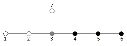
Figure 1: The Dynkin diagram of $E_{7}$. The Dynkin node labelled $i$ corresponds to the exceptional divisor $D_{i}$. The solid nodes are the ones we break to get the Standard Model gauge group and chiral matter. Node 3 (in gray) is broken by remainder flux while the others are broken by vertical flux.

Since only the vertical flux induces chiral matter, we can analyze the matter content by breaking $E_{7}\rightarrow SU(5)$, where the $\mathbf{56}$ breaks into a combination of $\mathbf{5},\mathbf{10}$, uncharged singlets and conjugate representations, and $\mathbf{133}$ includes these as well as the adjoint $\mathbf{24}$. Since the adjoint is non-chiral, the only chiral representations we expect for $G_{\rm SM}$ after the final breaking by remainder flux are the Standard Model representations

$$\left(\mathbf{3},\mathbf{2}\right)_{1/6}\,,\quad\left(\mathbf{3},\mathbf{1}\right)_{2/3}\,,\quad\left(\mathbf{3},\mathbf{1}\right)_{-1/3}\,,\quad\left(\mathbf{1},\mathbf{2}\right)_{1/2}\,,\quad\left(\mathbf{1},\mathbf{1}\right)_{1}\,.$$ (51)

As mentioned above, we expect anomaly cancellation separately from the matter arising from the $\mathbf{56},\mathbf{133}$ of $E_{7}$. Using Eq. (35), we indeed get SM chiral matter from vertical flux and the $\mathbf{56}$ with

$$\chi_{\left(\mathbf{3},\mathbf{2}\right)_{1/6}}^{\mathbf{56}}=\frac{1}{2}\left(3\Theta^{\mathbf{56}}_{4}+2\Theta^{\mathbf{56}}_{5}+\Theta^{\mathbf{56}}_{6}\right)\,,$$ (52)

where $\Theta^{\mathbf{56}}_{i}=-4\Theta_{iK_{B}}-3\Theta_{i\Sigma}$. Similarly, $\mathbf{133}$ also gives SM chiral matter with

$$\chi_{\left(\mathbf{3},\mathbf{2}\right)_{1/6}}^{\mathbf{133}}=-\left(3\Theta^{\mathbf{133}}_{4}+2\Theta^{\mathbf{133}}_{5}+\Theta^{\mathbf{133}}_{6}\right)\,,$$ (53)

where $\Theta^{\mathbf{133}}_{i}=\Theta_{iK_{B}}+\Theta_{i\Sigma}$. We see that only certain linear combinations of $\Theta_{i^{\prime}\alpha}$ appear in the chiral indices.

4.1.2 Exotic matter

To get SM chiral matter but not other representations $R^{\prime}$ of $G_{\rm SM}$, in the above procedure, it is important to choose the right embedding. For directly tuned $G_{\rm SM}$, it has been argued in TaylorTurnerGeneric that the model generically contains the SM matter fields and the representations $\left(\mathbf{3},\mathbf{1}\right)_{-4/3},\left(\mathbf{1},\mathbf{2}\right)_{3/2},\left(\mathbf{1},\mathbf{1}\right)_{2}$, while constructing representations $R^{\prime}$ other than these (defined as exotic matter representations) requires extensive amounts of fine-tuning. Here we will see that this is no longer the situation in the case of vertical flux breaking. As described in §3.1, we can get exotic $\mathrm{U}(1)$’s from simple vertical flux constraints, leading to many possible exotic representations $R^{\prime}$. Below we give such an example. Note that when $R^{\prime}$ other than SM matter representations are involved, the flux breaking may not realize all independent sets of chiral matter allowed by anomaly cancellation.

The directly tuned $G_{\rm SM}$ models containing generic matter, which includes the Standard Model representations, can be naturally unHiggsed into $\mathrm{SU}(4)\times\mathrm{SU}(3)\times\mathrm{SU}(2)$ models Raghuram:2019efb . It is interesting that the converse cannot be achieved from the perspective of $E_{7}$ flux breaking. As an example, we consider a flux breaking pattern from vertical flux that can be associated with the breaking route $E_{7}\rightarrow\mathrm{SU}\left(4\right)\times\mathrm{SU}\left(3\right)\times\mathrm{SU}\left(2\right)\rightarrow\mathrm{SU}\left(3\right)^{2}\times U\left(1\right)/\mathbb{Z}_{3}\rightarrow G_{\rm SM}$. Note that in this example we do not use remainder flux; all the breaking comes from vertical fluxes. This time we put the non-abelian part in nodes $1,4,5$, so we turn on nonzero $\Theta_{i^{\prime}\alpha}$ for $i^{\prime}=2,3,6,7$. Then we find that the $\mathrm{U}(1)$ charge is given by the generator

$$T=\frac{1}{2}T_{1}+T_{2}-\frac{1}{3}T_{4}-\frac{2}{3}T_{5}-T_{6}-T_{7}\,.$$ (54)

Therefore, we further impose $\Theta_{2\alpha}=\Theta_{6\alpha}+\Theta_{7\alpha}$ for all $\alpha$. This condition does not coincide with any root of $E_{7}$, so it really induces an exotic $\mathrm{U}(1)$.

As above, we analyze the breaking of $\mathbf{56}$ and $\mathbf{133}$ separately. The first observation is that $\mathbf{56}$ does not break into the generic matter representations that appear in directly tuned $G_{\rm SM}$ models. Instead, it breaks into the representations

$$\left(\mathbf{3},\mathbf{2}\right)_{1/6},\left(\mathbf{3},\mathbf{1}\right)_{5/3},\left(\mathbf{3},\mathbf{1}\right)_{-1/3},\left(\mathbf{1},\mathbf{2}\right)_{1/2},\left(\mathbf{1},\mathbf{1}\right)_{1},\left(\mathbf{3},\mathbf{1}\right)_{-4/3},\left(\mathbf{1},\mathbf{2}\right)_{3/2},\left(\mathbf{1},\mathbf{1}\right)_{2}\,.$$ (55)

That is, the right-handed up quark is replaced by the exotic $\left(\mathbf{3},\mathbf{1}\right)_{5/3}$, and there are various exotic representations that appear. There are three independent sets of chiral matter from anomaly cancellation. The chiral indices from flux breaking, however, only realize two of them:

$$\chi^{\mathbf{56}}=\Theta^{\mathbf{56}}_{3}\left(1,0,-3,2,-3,1,-1,2\right)+\frac{1}{2}\left(\Theta^{\mathbf{56}}_{6}+\Theta^{\mathbf{56}}_{7}\right)\left(3,-1,-6,3,-7,1,-2,5\right)\,.$$ (56)

Here the components of the vectors of fields correspond to the matter representations in Eq. (55) in the same order. The first set of of anomaly-canceling chiral matter fields only contains the generic matter representations that appear in directly tuned $G_{\rm SM}$ models, while the second set involves the exotic $\left(\mathbf{3},\mathbf{1}\right)_{5/3}$.

The analysis for $\mathbf{133}$ is similar. Under the prescribed breaking route it breaks into

$$\left(\mathbf{3},\mathbf{2}\right)_{1/6},\left(\mathbf{3},\mathbf{2}\right)_{7/6},\left(\mathbf{3},\mathbf{2}\right)_{-11/6},\left(\mathbf{3},\mathbf{1}\right)_{2/3},\left(\mathbf{3},\mathbf{1}\right)_{-1/3},\left(\mathbf{3},\mathbf{1}\right)_{-4/3},$$

$$\left(\mathbf{3},\mathbf{1}\right)_{5/3},\left(\mathbf{1},\mathbf{2}\right)_{1/2},\left(\mathbf{1},\mathbf{2}\right)_{3/2},\left(\mathbf{1},\mathbf{1}\right)_{1},\left(\mathbf{1},\mathbf{1}\right)_{2},\left(\mathbf{1},\mathbf{1}\right)_{3}\,.$$ (57)

This gives many more exotic matter representations than $\mathbf{56}$, which can have nontrivial chiral indices for generic fluxes. Again, only two of the allowed independent sets of chiral matter are realized. The chiral indices are

$$\chi^{\mathbf{133}}= \Theta^{\mathbf{133}}_{3}\left(-1,0,0,0,0,1,1,1,0,1,-1,0\right)$$

$$+\left(\Theta^{\mathbf{133}}_{3}+\Theta^{\mathbf{133}}_{6}+\Theta^{\mathbf{133}}_{7}\right)\left(0,2,1,-3,3,-4,2,-6,1,4,-2,1\right)\,,$$ (58)

following the above order. The first set contains only those $R^{\prime}$ from both $\mathbf{56}$ and $\mathbf{133}$. Note that while the $\mathbf{56}$ alone does not generate all states in the Standard Model spectrum, the missing states are supplied by the $\mathbf{133}$. On the other hand, there is no choice of fluxes that gives only SM matter and no exotics: the second set of representations from $\mathbf{133}$ is the only place that some exotic matter fields like $\left(\mathbf{1},\mathbf{1}\right)_{3}$ appear, so the fluxes generating this family must cancel in the absence of exotic matter. But this is the only combination that includes the field $\left(\mathbf{3},\mathbf{1}\right)_{2/3}$, so we cannot get the full Standard Model chiral matter spectrum from this construction without at least some exotics.

In conclusion, while the flux constraints are equally simple in many constructions, choosing the incorrect embedding of $G_{\rm SM}$ into $E_{7}$ can lead to a variety of exotic chiral matter fields. These matter representations are generically present since there are many more than 4 choices of $\mathrm{U}(1)$ in $G_{\rm SM}$ that can be embedded into $E_{7}$. For many of these choices, unlike the case just analyzed here, there may actually be no resulting fields in some of the Standard Model representations. In others, like this one, all of the SM representations may appear along with some exotics; while in this specific case we can show that no flux combination is possible that gives just SM matter without exotics, it is possible that for other U(1) choices, a judicious tuning of fluxes may cancel the chiral multiplicities of all exotic matter fields, still allowing for an SM construction with the expected matter fields and no exotics, but we leave a full consideration of this question for further research.

4.2 Solving the flux constraints

Now we turn back to the construction of the Standard Model gauge group and chiral matter from §4.1.1. Although we have obtained the chiral index in terms of $\Theta_{i^{\prime}\alpha}$, we still need to solve the flux constraints and express everything in terms of flux parameters $\phi$.

There is a subtlety before breaking $E_{7}$. Most $E_{7}$ models have codimension-3 singularities with degree $(4,6,12)$. Such singularities can no longer be simply interpreted as Yukawa couplings. The fiber becomes non-flat at these points and supports an extra vertical flux. It also seems to correspond to extra strongly coupled (chiral) degrees of freedom, possibly M5-branes wrapping non-flat fibers Candelas:2000nc ; Lawrie:2012gg ; Jefferson:2021bid . Although $E_{7}$ itself does not support any chiral matter, after flux breaking the extra flux may induce more chiral matter which is not covered by our formalism. This will be studied in 46 . For realistic SM-like models, we simply set such extra flux to vanish, so all the flux we consider is for flux breaking.

It is now straightforward to solve the flux constraints by considering independent $S_{i\alpha}$. Recall from (24) that $\Theta_{i\alpha}=-\Sigma\cdot D_{\alpha}\cdot D_{\beta}\kappa^{ij}\phi_{j\beta}$. For independent $S_{i\alpha}$, the triple intersection form $M^{B}_{\alpha\beta}=\Sigma\cdot D_{\alpha}\cdot D_{\beta}$ on $B$ is invertible. The solution to $\Theta_{1\alpha}=\Theta_{2\alpha}=\Theta_{3\alpha}=\Theta_{7\alpha}=0$ is simply

$$\phi_{1\alpha}=2n_{\alpha}\,,\quad\phi_{2\alpha}=4n_{\alpha}\,,\quad\phi_{3\alpha}=6n_{\alpha}\,,\quad\phi_{4\alpha}=5n_{\alpha}\,,\quad\phi_{7\alpha}=3n_{\alpha}\,,$$ (59)

with $\phi_{5\alpha},\phi_{6\alpha}$ arbitrary, but we pick sufficiently generic $\phi_{5\alpha},\phi_{6\alpha}$ such that the resulting gauge group does not get further enhanced. These fluxes give

$$\Theta_{4\alpha}=M^{B}_{\alpha\beta}(\phi_{5\beta}-4n_{\beta})\,,\quad\Theta_{5\alpha}=M^{B}_{\alpha\beta}(5n_{\beta}-2\phi_{5\beta}+\phi_{6\beta})\,,\quad\Theta_{6\alpha}=M^{B}_{\alpha\beta}(\phi_{5\beta}-2\phi_{6\beta})\,.$$ (60)

The flux quantization condition is satisfied by integer $\phi_{i\alpha}$, hence integer $n_{\alpha}$ when $c_{2}(\hat{Y})$ is even. The D3-tadpole condition is satisfied when $\phi_{i\alpha}$ are sufficiently small. Now Eq. (52) and (53) give

$$\chi_{(\mathbf{3},\mathbf{2})_{1/6}}=\Sigma\cdot(6K_{B}+5\Sigma)\cdot D_{\alpha}n_{\alpha}\,.$$ (61)

This is one of the main results in this paper. The independence of the chiral multiplicity from the parameters $\phi_{5\alpha},\phi_{6\alpha}$ can be understood from the fact that these fluxes do not hit the roots of the preserved part of the gauge group. Note that $-(6K_{B}+5\Sigma)$ is the class of the coefficient of $s^{5}z^{6}$ in the $E_{7}$ Tate model BershadskyEtAlSingularities ; KatzEtAlTate . Intersecting it with $C_{\mathbf{56}}$ gives the codimension-3 singularities.

We see that in a generic basis for the base divisors $D_{\alpha}$, there are $r$ (see §3.1) quantized flux parameters contributing to a single chiral index, and the chiral index has a linear Diophantine structure. This is unlike the case in directly tuned $G_{\rm SM}$ models, where the chiral index is controlled by a single flux parameter with a large constant factor, and either specific geometries must be chosen, or a better understanding of the quantization conditions discussed in §2.3 must be achieved, to make the chiral index as small as 3. In our case, generically the intersection numbers $\Sigma\cdot(6K_{B}+5\Sigma)\cdot D_{\alpha}$ have no common factors, and the chiral index can be any integer. A generic flux configuration has both positive and negative $n_{\alpha}$ with small magnitudes (due to the large number of flux directions that can contribute to the tadpole as discussed in §2.3), making the terms in Eq. (61) cancel and naturally leading to a small chiral index. Heuristically, if we sample $\chi_{(\mathbf{3},\mathbf{2})_{1/6}}$ throughout the landscape, we expect a distribution peaking at $\chi=0$ and decaying as $\chi$ becomes large Andriolo:2019gcb . Therefore, $\chi=3$ is a natural solution although it may not be the most preferred. In conclusion, Eq. (61) is favored by phenomenology.

There may be also some rare cases where the triple intersection numbers have a common factor. Most probably the common factor forbids the possibility of $\chi=3$, but if the common factor is 3, interestingly $\chi=3$ becomes both the minimal and natural nontrivial chiral spectrum.

The appearance of a nontrivial minimal multiplicity, and other aspects of multiplicity quantization, can be understood in terms of intersection theory on the base $B$, combined with the structure of the $E_{7}$ lattice. The intersection product $C=\Sigma\cdot(6K_{B}+5\Sigma)$ is a curve in integer homology of the base $B$. For generic choices of characteristic data, we expect that this curve will be primitive, in which case Poincaré duality asserts that there is a divisor $D^{\prime}=D_{\alpha}n^{\prime}_{\alpha}$ with $C\cdot D^{\prime}=1,n^{\prime}_{\alpha}\in\mathbb{Z}$. This is the generic case described above where there are no common factors and the chiral index can be any integer. Thus, in some sense the flux associated with the chiral index can be characterized by a single parameter $\lambda$, with $n_{\alpha}=\lambda n^{\prime}_{\alpha}$. On the other hand, a full treatment of the proper basis for fluxes would involve identifying flux directions with minimal tadpole contribution, which we do not investigate further here. When $C=mC^{\prime}$ is not primitive but is an integer multiple of a primitive curve $C^{\prime}$, this corresponds to the situation where there are common factors and there is a non-unit minimal multiplicity for $\chi$; the case where $\chi=3$ is minimal corresponds to the situation where $m=3$.

It is interesting that more generally we can consider fluxes in $H^{4}(\hat{Y},\mathbb{Z})$ that may lead to fractional values of $n_{\alpha}$. Since $H^{4}(\hat{Y},\mathbb{Z})$ has a unimodular intersection form, we expect that there may be fluxes in $H^{4}(\hat{Y},\mathbb{Z})$ with fractional vertical components $n_{\alpha}$, when the fluxes $\phi_{i\alpha}$ lie in the dual of the root lattice (i.e., the weight lattice) of $E_{7}$. From the form of the $E_{7}$ lattice, the only non-integer fluxes allowed have half-integer entries for $\phi_{4\alpha},\phi_{6\alpha},\phi_{7\alpha}$. This results in half-integer $n_{\alpha}$ in Eq. (59) and naively appears to lead to half-integer multiplicities in Eq. (61). The multiplicities should be, however, guaranteed to be integers from the structure of $H^{4}(\hat{Y},\mathbb{Z})$. The explicit form of $H^{4}(\hat{Y},\mathbb{Z})$ is not yet fully elucidated, as discussed in §2.3, which makes these issues a bit subtle, and we leave a more detailed investigation of such situations to further work.

There are still other flux constraints remaining such as primitivity. Solving these constraints will be demonstrated in Section 6.

5 Breaking other gauge groups

So far we have focused on the breaking $E_{7}\rightarrow G_{\rm SM}$, while among the rigid gauge groups, $E_{6}$ and $E_{8}$ can also be broken into $G_{\rm SM}$. $E_{6}$ has been one of the traditional GUT groups, so its breaking is less novel than $E_{7}$’s. Flux breaking of (non-rigid) $E_{6}$ F-theory models has been described in the dual heterotic framework in Chen:2010tg . On the other hand, $E_{6}$ also appears in a significant portion of the landscape, and we therefore generalize our construction to $E_{6}$ for completeness. $E_{8}$ is clearly the most abundant exceptional gauge group in the landscape, but unfortunately our formalism does not work for $E_{8}$ for several reasons. Below we discuss these two gauge groups separately.

5.1 $E_{6}$

It is clear that the above construction for $E_{7}$ also works for $E_{6}$, since we can first break $E_{7}$ down to $E_{6}$ in our breaking by vertical flux. The generalization to $E_{6}$, however, is more nontrivial since $E_{6}$ itself supports chiral matter without flux breaking. There are more flux parameters $\phi_{ij}$ to turn on, and both terms in Eq. (35) contribute to the chiral indices. Although as discussed before the two terms in Eq. (35) are independent contributions controlled by different flux parameters, the flux configuration itself becomes more nontrivial due to flux quantization. This will be explained below.

Although we expect the middle intersection form on vertical fluxes (22) as well as the physics to be resolution-independent, in practice it is useful to work with a certain resolution, and extract resolution-independent information from the results. Here we choose the resolution studied in Esole:2017kyr ; Bhardwaj_2019 ; Jefferson:2021bid , which for completeness we review in Appendix C. The exceptional divisors and the broken directions are described as in Figure 2.

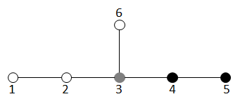
Figure 2: The Dynkin diagram of $E_{6}$. The Dynkin node labelled $i$ corresponds to the exceptional divisor $D_{i}$. The solid nodes are the ones we break to get the Standard Model gauge group and chiral matter. Node 3 (gray) is broken by remainder flux while the others are broken by vertical flux.

The result in Jefferson:2021bid shows that when the gauge group is unbroken, there is a chiral index for the $E_{6}$ fundamental $\mathbf{27}$, given by

$$\chi_{\mathbf{27}}=\Theta_{24}\,.$$ (62)

Following the procedure in Section 3.2, we find that the matter surface $S_{0}(\mathbf{27})$ is

$$S_{0}(\mathbf{27})=D_{2}\cdot D_{4}+\frac{1}{3}\pi^{*}(3K_{B}+2\Sigma)\cdot(-D_{1}+D_{2}+2D_{4}+D_{5})\,,$$ (63)

where the class $(3K_{B}+2\Sigma)$ appears in the matter curve $C_{\mathbf{27}}=-\Sigma\cdot(3K_{B}+2\Sigma)$.

Recall that both the flux configuration and chiral indices can be separated into parts that preserve or break the gauge group. We now decompose $G_{4}=G_{4}^{p}+G_{4}^{b}$, where $G_{4}^{p}$ lives in the directions in $M_{\mathrm{phys}}$ and preserves the gauge group, while $G_{4}^{b}$ is the gauge-breaking flux. Correspondingly we define the flux parameters $\phi^{p},\phi^{b}$ and chiral indices $\chi^{p},\chi^{b}$. By solving the flux constraints, $G_{4}^{p}$ is given by

$$G_{4}^{p}=\phi_{24}^{p}\left[S_{0}(\mathbf{27})\right]\,,$$ (64)

inducing

$$\chi^{p}_{(\mathbf{3},\mathbf{2})_{1/6}}=\chi_{\mathbf{27}}=\frac{1}{3}\Sigma\cdot(3K_{B}+2\Sigma)\cdot(6K_{B}+5\Sigma)\phi_{24}^{p}\,.$$ (65)

As expected, this chiral index is controlled by a single flux parameter $\phi^{p}_{24}$. We discuss the detailed quantization condition on this parameter below, but note that $K_{B}\cdot\Sigma\cdot\Sigma$ is always even, by the Hirzebruch-Riemann-Roch theorem for surfaces, so the chiral multiplicity is always an integer when $\phi_{24}^{p}$ is a multiple of 3/2.

Now we turn to $G_{4}^{b}$. Here we follow the breaking route used in Section 4.2. In principle, we can apply the same procedure as in Section 4 to obtain $G_{4}^{b}$ and $\chi^{b}$, but there is a faster way using the result for $E_{7}$. We can first break $E_{7}$ down to $E_{6}$ by removing node 6 in Figure 1. Note that $\phi_{6\alpha}$ in the $E_{7}$ model are completely independent of other flux parameters and do not contribute to the chiral indices. Therefore, $G_{4}^{b}$ for $E_{6}$ is the same as that for $E_{7}$ by ignoring node 6 in $E_{7}$. That is

$$\phi^{b}_{1\alpha}=2n_{\alpha}\,,\quad\phi^{b}_{2\alpha}=4n_{\alpha}\,,\quad\phi^{b}_{3\alpha}=6n_{\alpha}\,,$$

$$\phi^{b}_{4\alpha}=5n_{\alpha}\,,\quad\phi^{b}_{6\alpha}=3n_{\alpha}\,,$$ (66)

where $\phi^{b}_{5\alpha}$ is arbitrary. Therefore, the chiral index from flux breaking is

$$\chi^{b}_{(\mathbf{3},\mathbf{2})_{1/6}}=\Sigma\cdot(6K_{B}+5\Sigma)\cdot D_{\alpha}n_{\alpha}\,,$$ (67)

which is exactly the same as Eq. (61). The total chiral index is then $\chi=\chi^{p}+\chi^{b}$. Despite the extra $\chi^{p}$, with the inclusion of $\chi^{b}$ it is qualitatively the same as that in $E_{7}$ models.

So far $\phi^{p}$ and $\phi^{b}$ are totally separated, but it becomes more interesting when flux quantization is considered. First, in $E_{6}$ models it is unavoidable to have a non-even $c_{2}(\hat{Y})$. Using the techniques in Jefferson:2021bid , we find that for our choice of resolution (in terms of independent surfaces)

$$\left[c_{2}(\hat{Y})\right]= \left[c_{2}(B)\right]+11\pi^{*}K_{B}^{2}+\left(-12D_{0}+17D_{1}+27D_{2}+30D_{3}+24D_{4}+11D_{5}+14D_{6}\right)\cdot\pi^{*}K_{B}$$

$$+\left(6D_{1}+8D_{2}+6D_{3}+6D_{4}+2D_{5}+2D_{6}\right)\cdot\pi^{*}\Sigma+D_{2}\cdot D_{4}\,.$$ (68)

Note that $\left[c_{2}(B)\right]+\pi^{*}K_{B}^{2}$ is always even Collinucci:2010gz . Note also from the form of Eq. (63) that the part of $c_{2}$ that is odd precisely contributes to a half-integer contribution to $G_{4}^{p}$ and does not necessitate breaking of the $E_{6}$. If the gauge group is unbroken i.e. $G_{4}^{b}=0$, we see that flux quantization generically requires $\phi_{24}^{p}=3(2k+1)/2$ for some integer $k$. (As noted above, this always gives integer chiral multiplicity since $K_{B}\cdot\Sigma\cdot\Sigma$ is always even.) The situation, however, is different if both $G_{4}^{p}$ and $G_{4}^{b}$ are present. The crucial point is that flux quantization only applies to the total flux $G_{4}$, allowing more flux configurations if we look at one of the sectors only. In particular, now $\phi_{24}^{p}$ can be any half-integer, as long as appropriate fractional $\phi_{i\alpha}$ are turned on such that the total flux is correctly quantized. Therefore, the presence of gauge-breaking flux enlarges the possibilities of matter surface flux, although they contribute to chiral indices independently.

5.2 $E_{8}$

It is tempting to apply our formalism to $E_{8}$ models. Nevertheless, these models have very different physics from $E_{7},E_{6}$ models, and the direct construction of Standard Model-like vacua from flux breaking of rigid $E_{8}$ factors fails for various reasons.

The first reason is that an $E_{8}$ model generically contains codimension-2 $(4,6)$ singularities. While this type of singularity in 4D has not been completely understood, it is believed to be parallel to the story in 6D F-theory models. There, a simple physical interpretation of these singularities is obtained by blowing up the locus into the tensor branch till the singularities are within the minimality bound i.e. degree $<(4,6,12)$. The origin of the tensor branch corresponds to shrinking the resulting exceptional divisors to zero volume, giving a strongly coupled limit of the model. D3-branes wrapping these exceptional divisors also become tensionless strings in the low-energy theory. All these signal the presence of strongly coupled superconformal sectors HeckmanMorrisonVafa ; DelZotto:2014hpa ; Apruzzi:2018oge . These extra degrees of freedom, called conformal matter, are not covered by our formalism for analyzing flux breaking.

Still, there are $E_{8}$ models without these kinds of singularities and naively our formalism should work in such cases. The second reason, however, that these geometries are problematic is that the condition for the absence of conformal matter is that the codimension-2 singularity has trivial homology class i.e. $\Sigma\cdot(6K_{B}+5\Sigma)=0$. Surprisingly, using Eq. (61) this immediately implies that no chiral matter can be induced, even if we break $E_{8}\rightarrow G_{\rm SM}$. It remains interesting to find a reason behind this apart from direct computations.

All this seem to suggest that the class of SM-like models we have constructed may still not be the largest class in the landscape. In particular, the F-theory geometry with the most flux vacua contains many factors of $E_{8}$, but no factors of $E_{7},E_{6}$ and does not support our formalism TaylorWangVacua . In principle, the most generic SM matter should come from the strongly coupled matter in $E_{8}$. Some initial investigation into studying the 4D spectrum from strongly coupled $E_{8}$ matter in the context of E-string theory is described in TianWangEString .

6 An explicit example

The above construction of SM gauge group and chiral matter can be done on a large class of bases containing rigid or tuned $E_{7},E_{6}$ factors. For the rigid case, we need a non-toric base such that there can be a rigid divisor supporting hypercharge flux. In this section, we provide an explicit example of such a construction, with three generations of SM chiral matter as the minimal and preferred chiral matter content. Since the $E_{7}$ models require a more involved construction with $r\geq 4$, below we construct rigid $E_{6}$ with $r=3$. As shown below, the gauge divisor is a del Pezzo surface $dP_{4}$, so the model has a limit where gravity is fully decoupled BeasleyHeckmanVafaII .

We choose a base $B$ through the following procedure: first consider $A=\mathbb{P}^{1}\times\mathbb{F}_{1}$ where $\mathbb{F}_{1}$ is the Hirzebruch surface. Then $B$ is a certain hypersurface in an ambient space $X$ that is a $\mathbb{P}^{1}$-bundle over $A$ with a certain normal bundle. This example is a generalization of an example of a geometry supporting remainder flux in Braun:2014pva ; more generally we can similarly analyze any hypersurface $B$ in a toric fourfold $X$ as long as $B$ is ample. In the explicit example we consider here, both vertical and remainder fluxes are incorporated, and all flux constraints can be explicitly solved.

Let us first construct the ambient space $X$. To construct a model with $r\geq 3$ (see §3.1), we need to start with a threefold $A$ with $h^{1,1}\geq 3$. As an example with $h^{1,1}(A)=3$, we choose $A$ to be $\mathbb{P}^{1}\times\mathbb{F}_{1}$. Within $\mathbb{F}_{1}$, we denote $s$ as the $\mathbb{P}^{1}$ section and $f$ as the $\mathbb{P}^{1}$ fiber. Then the intersection numbers are $f^{2}=0,f\cdot s=1,s^{2}=-1$. Now on $A$, we denote $\sigma$ as the $\mathbb{F}_{1}$ section and $S,F$ as the $\mathbb{P}^{1}$ product with $s$ and $f$ respectively. Then the anticanonical class of $A$ is $-K_{A}=2\sigma+2S+3F$. The nonzero intersection numbers are:

$$\sigma\cdot S\cdot F=1\,,\;\sigma\cdot S^{2}=-1\,.$$ (69)

Finally we can describe $X$ as a $\mathbb{P}^{1}$-bundle over $A$. We denote $\sigma_{A}$ as the section and $F_{\sigma},F_{S},F_{F}$ as the fibers along $\sigma,S,F$ respectively. Let the normal bundle be $N_{A}=-a\sigma-bS-cF$ where $a,b,c\in\mathbb{Z}_{\geq 0}$. Then its anticanonical class is $-K_{X}=2\sigma_{A}+(a+2)F_{\sigma}+(b+2)F_{S}+(c+3)F_{F}$. The intersection numbers can be calculated using Eq. (69) and the relations $\sigma_{A}\cdot(\sigma_{A}+aF_{\sigma}+bF_{S}+cF_{F})=0$. Note that with the below choice of $N_{A}$, $X$ is a smooth, projective toric variety with a unique triangulation.

We then choose the base as a hypersurface in $X$ with irreducible class $B=\sigma_{A}+(a+1)F_{\sigma}+(b+1)F_{S}+(c+2)F_{F}$. By abuse of notation, we use $B$ to denote both the base and its divisor class in $X$. By adjunction we have $-K_{B}=B\cdot(\sigma_{A}+F_{\sigma}+F_{S}+F_{F})$. As shown below, $B$ is strictly inside the Kähler cone of $X$, so $B$ is ample in $X$. By Lefschetz’s hyperplane theorem, we then have the isomorphism $H^{1,1}\left(B,\mathbb{Z}\right)\cong H^{1,1}\left(X,\mathbb{Z}\right)$. In other words, divisors on $B$ are spanned by the intersections $B\cdot\sigma_{A},B\cdot F_{\sigma},B\cdot F_{S},B\cdot F_{F}$. The intersection numbers relevant to our purpose are

$$B\cdot\sigma_{A}\cdot F_{\sigma}^{2}=0\,,\;B\cdot\sigma_{A}\cdot F_{\sigma}\cdot F_{S}=1\,,\;B\cdot\sigma_{A}\cdot F_{\sigma}\cdot F_{F}=1$$

$$B\cdot\sigma_{A}\cdot F_{S}\cdot F_{F}=1\,,\;B\cdot\sigma_{A}\cdot F_{S}^{2}=-1\,,\;B\cdot\sigma_{A}\cdot F_{F}^{2}=0\,.$$ (70)

Now consider the gauge divisor $\Sigma=B\cdot\sigma_{A}=\sigma_{A}\cdot(F_{\sigma}+F_{S}+2F_{F})$. To determine the rigid gauge group on $\Sigma$, we calculate

$$-K_{\Sigma}=B\cdot\sigma_{A}\cdot\left(F_{\sigma}+F_{S}+F_{F}\right)=\sigma_{A}\cdot\left(2F_{\sigma}\cdot F_{S}+3F_{\sigma}\cdot F_{F}+2F_{S}\cdot F_{F}\right)\,,$$ (71)

$$N_{\Sigma}=B\cdot\sigma_{A}^{2}=-\sigma_{A}\cdot\left((a+b)F_{\sigma}\cdot F_{S}+(2a+c)F_{\sigma}\cdot F_{F}+(b+c)F_{S}\cdot F_{F}\right)\,.$$ (72)

By the conditions in §2.2, we choose $(a,b,c)=(3,3,3)$ such that $\Sigma$ is a rigid divisor supporting a rigid $E_{6}$. Note that with this choice of $N_{A}$, $C_{\mathbf{27}}$ is trivial and all the matter is in the $E_{6}$ adjoint $\mathbf{78}$ before flux breaking. Note also that with this choice $N_{\Sigma}=3K_{\Sigma}$ is divisible by 3, so the curve $C=\Sigma\cdot(6K_{B}+5\Sigma)$ appearing in Eq. (67) is not primitive but takes the form $C=3C^{\prime}$ as discussed in §4.2, and we expect chiral multiplicities that are multiples of 3. Note further that we have not ruled out fully the possibility of increased enhancement over curves in the base, which might in principle give rise to additional surfaces. Even if this occurs, however, it should not be relevant for our construction as we can simply keep any associated additional fluxes that may arise to vanish. For future work and more general constructions, however, it would be useful to develop more completely the methodology for analyzing the structure of hypersurface bases of this general kind.

We can solve the flux constraints after determining the geometry. First we focus on vertical flux. Let us analyze the constraint from primitivity. The independent $S_{i\alpha}$ are $S_{i(B\cdot F_{\sigma})},S_{i(B\cdot F_{S})},S_{i(B\cdot F_{F})}$, while $S_{i\Sigma}$ is a linear combination of the former three. Using the intersection numbers, we see that the triple intersection form $M^{B}_{\alpha\beta}$ has one positive and two negative directions, so primitivity can be satisfied. As explained in Section 3.3, we focus on the Kähler form of the base $J_{B}$, which can be expanded using a basis of base divisors (recall that in this case as noted above, $H^{1,1}\left(B,\mathbb{Z}\right)\cong H^{1,1}\left(X,\mathbb{Z}\right)$):

$$\left[J_{B}\right]=B\cdot\left(t_{1}F_{F}+t_{2}\left(F_{S}+F_{F}\right)+t_{3}F_{\sigma}+t_{4}\left(\sigma_{A}+3F_{\sigma}+3F_{S}+3F_{F}\right)\right)\,,$$ (73)

where $t_{1},t_{2},t_{3},t_{4}$ are linear combinations of Kähler moduli, and may be negative inside the Kähler cone of $B$ in general. While determining the exact Kähler cone of a hypersurface in a toric variety can be subtle, the Kähler cone of $B$ must contain that of $X$ Demirtas:2018akl . For simplicity, we look for a solution of the primitivity constraints in the Kähler cone of $X$ only. First, the Kähler cone of $X$ can be obtained from the Mori cone, which is spanned by $F_{\sigma}\cdot F_{S}\cdot F_{F},\sigma_{A}\cdot F_{\sigma}\cdot F_{S},\sigma_{A}\cdot F_{\sigma}\cdot F_{F},\sigma_{A}\cdot F_{S}\cdot F_{F}$. By computing the dual cone, we see that the interior of the Kähler cone of $X$ corresponds to $t_{1},t_{2},t_{3},t_{4}>0$. Now primitivity implies that for all $i$

$$t_{1}(\phi_{i\sigma}+\phi_{iS})+t_{2}(2\phi_{i\sigma}+\phi_{iF})+t_{3}(\phi_{iS}+\phi_{iF})=0\,.$$ (74)

To determine the chiral matter spectrum, we first focus on $n_{\alpha}$. There must be a pair of coefficients of $t_{a}$ with opposite signs, which places constraints on the possible $n_{\alpha}$.

Now we consider the chiral index. First, $\phi^{p}$ and Eq. (65) vanish since $C_{\mathbf{27}}$ is trivial. Eq. (67) then gives

$$\chi_{\left(\mathbf{3},\mathbf{2}\right)_{1/6}}=-3(2n_{\sigma}+n_{S}+2n_{F})\,,$$ (75)

where $n_{I}=n_{(B\cdot F_{I})}$. As discussed before, it is natural to consider small $\phi_{i\alpha}$. To fulfill flux quantization as in Section 5.1, we turn on integer $n_{\alpha}$. One of the minimal flux configurations satisfying the flux constraints has $(n_{\sigma},n_{S},n_{F})=(-1,1,0)$, hence gives $\chi=3$ as the minimal and preferred chiral spectrum.

We now turn to remainder flux. It can be shown that $\Sigma$ is a del Pezzo surface $dP_{4}$ and supports remainder flux. First notice that $\Sigma$ is a hypersurface in $A$ with class $\sigma+S+2F$. In other words, $\Sigma$ is the vanishing locus

$$xP+yP^{\prime}=0\,,$$ (76)

in $A$, where $P,P^{\prime}$ are sections of $\mathcal{O}_{A}(S+2F)$, and $x,y$ are the homogeneous coordinates of the $\mathbb{P}^{1}$ in $A$. For generic points in the $\mathbb{F}_{1}$, Eq. (76) has a unique solution, representing a single point in $\mathbb{P}^{1}$. On the other hand, there are $(s+2f)^{2}=3$ points in $\mathbb{F}_{1}$ such that $P=P^{\prime}=0$, and Eq. (76) represents the whole $\mathbb{P}^{1}$. Therefore, the geometry of $\Sigma$ is $\mathbb{F}_{1}$ blown up in 3 generic points i.e. a $dP_{4}$, where the projection $A\rightarrow\mathbb{F}_{1}$ gives the blow-down map $\Sigma\rightarrow\mathbb{F}_{1}$.

To construct the remainder flux, notice that the three exceptional curves on $\Sigma$ from blowing up $\mathbb{F}_{1}$ (denoted by $e_{1},e_{2},e_{3}$) are all $\mathbb{P}^{1}$ fibers in $A$, which have class $S\cdot F$. Under the inclusion map $\iota:\Sigma\rightarrow B$, we then have $\iota_{*}e_{i}=\sigma_{A}\cdot F_{S}\cdot F_{F}$ for all $i=1,2,3$. Therefore, we can choose e.g. $C_{\mathrm{rem}}=e_{1}-e_{2}$ and turn on the remainder flux

$$G_{4}^{\mathrm{rem}}=\left[\left(D_{Y}+\phi_{4r}D_{4}+\phi_{5r}D_{5}\right)|_{C_{\mathrm{rem}}}\right]\,,$$ (77)

where the first term is the hypercharge flux in Eq. (50) and the other two terms with free flux parameters $\phi_{4r},\phi_{5r}$ do not affect the gauge group. Notice that when $\phi_{4r}=4$, it is known that this flux removes the exotic vector-like $(\mathbf{3},\mathbf{2})_{-5/6}$ BeasleyHeckmanVafaII , avoiding a number of phenomenological inconsistencies such as part of proton decay. Importantly, this removal can be achieved without the complication of using fractional line bundles, which must be used in traditional $\mathrm{SU}(5)$ models, due to more flux parameters. This is parallel to how the Diophantine structure in vertical flux enables much more possibilities for chiral indices. These further phenomenological features of our models will be studied in a future publication. In the analysis below, we keep this choice of $\phi_{4r}$.

For consistency, we still need to study the tadpole condition, see Eq. (9). First we specify the remaining flux parameters $\phi_{5\alpha},\phi_{5r}$. As an example with small tadpole, we choose $(\phi_{5F_{\sigma}},\phi_{5F_{S}},\phi_{5F_{F}},\phi_{5r})=(-3,2,1,2)$. The total flux is then given by these four parameters, the vertical flux in Eq. (66), and the remainder flux in Eq. (77) with $\phi_{4r}=4$. The vertical flux consistently stabilizes the Kähler moduli at $2t_{1}=2t_{2}=t_{3}$. The total tadpole is

$$\frac{1}{2}\int_{\hat{Y}}G_{4}^{\mathrm{vert}}\wedge G_{4}^{\mathrm{vert}}+\frac{1}{2}\int_{\hat{Y}}G_{4}^{\mathrm{rem}}\wedge G_{4}^{\mathrm{rem}}=13+6=19\,.$$ (78)

Here we have naturally extended Eq. (21) to remainder flux, since the intersections are all localized on $\Sigma$. Using the technique in Esole:2017kyr , we find that $\chi(\hat{Y})=2088$. Since $\chi(\hat{Y})/24=87>19$, the tadpole condition is satisfied.

We would like to emphasize that although we have chosen an explicit global example here, the analysis is purely local. The same breaking pattern and matter spectrum are expected whenever there is a $\Sigma$ in $B$ with the same geometry and normal bundle. This is analogous to 6D F-theory models, in which any curve of self-intersection $-6$ supports a rigid $E_{6}$ MorrisonTaylorClusters . We expect that many of the F-theory threefold bases contain the above local structure. Moreover, there are lots of local structures throughout the landscape that support the same flux breaking. Therefore, our construction provides a large class of models with SM gauge group and chiral matter, with much less fine-tuning that is needed for other known constructions.

7 Conclusion and further questions

7.1 Summary of results

In this paper, we have described a large class of Standard Model-like models with the right gauge group and chiral matter spectrum, using the framework of F-theory compactifications. These models originate from rigid $E_{7}$ (covered briefly in Li:2021eyn ) or $E_{6}$ gauge symmetries, which are ubiquitous in the string landscape and do not require any fine-tuning of moduli. In particular, the UV physics of string theory allows us to use $E_{7}$, in addition to the traditional $E_{6}$, as a GUT group. The same construction can be carried out on many (but non-toric) F-theory threefold bases that contain rigid $E_{7}$ or $E_{6}$ local structures. Due to such genericity, we expect that this is a natural way for the Standard Model to arise in the landscape. Although we do not have an exact quantification, we believe these models should be more generic than tuned SM-like models in the landscape.

Remarkably, these models also enjoy the advantage of typically having small chiral indices. While the chiral indices in tuned SM-like models are usually too large unless very specific geometries are considered, or the subtle flux quantization issues discussed in §2.3 are managed, the chiral indices in our models have a linear Diophantine structure that naturally leads to small integers for typical geometries. As a result, three generations of SM chiral matter can be easily realized in our models. In particular, a subset of them have $\chi=3$ as the minimal or preferred matter content. This is favored by phenomenology. We hope that this large class of SM-like constructions can shed some light on where our Universe sits in the string landscape, and whether it is a natural solution in the landscape.

The main tool we have used to achieve the above results is gauge symmetry breaking with both vertical and remainder fluxes. This is an efficient way to build models, as it breaks the gauge group and induces chiral matter at the same time. While this idea is not new, we have developed it here in depth to give a systematic procedure to describe the flux breaking from any $G$ to any $G^{\prime}$ on almost any base, and calculate the chiral spectrum induced by the vertical flux. All these calculations can be done using simple formulas and give results that are manifestly resolution-independent, with the base geometry and group theory data as the only input. A remarkable fact from this procedure is that even if $G$ does not support any chiral matter, generically a chiral spectrum is still induced if $G^{\prime}$ supports chiral matter. This is why we can use $G=E_{7}$ in our SM-like models. The only exception we find is $G=E_{8}$. The procedure developed here is a byproduct of our study of SM-like models, and should be useful for other types of F-theory model building in the future.

7.2 Further questions

As mentioned at the beginning of the paper, although the models we have constructed here have the right gauge group and chiral matter spectrum, they are far from complete in realizing the full details of the Standard Model in string theory. More work is needed to understand the full matter spectrum including vector-like fields, Yukawa couplings, questions related to proton decay, etc. Many other more general questions can also be asked, regarding both theoretical and phenomenological aspects of these models. Examples include:

• One interesting feature of our formalism of flux breaking is that it intrinsically relies on the non-perturbative physics of F-theory. The gauge-breaking flux we turn on does not have any immediately obvious description in the low-energy theory. In particular, the approach of inducing chiral matter with the flux cannot be realized in the framework of field theory in any known way. Although the broken gauge group and chiral matter spectrum are certainly low-energy observables, they do not give full information on the flux configuration, and the original $E_{7}$ or $E_{6}$ gauge group does not seem to be apparent in any clear way in the low-energy theory. To gain a more complete picture, it would be interesting to understand the structure of these models better from the low-energy perspective and/or in the dual heterotic framework.

• In a string compactification compatible with observations, the moduli must be stabilized. In F-theory, the stabilization of complex structure moduli is done by turning on horizontal flux, inducing a superpotential for the moduli. This flux is orthogonal to vertical flux and does not affect the matter spectrum. In models with tuned gauge groups, however, some complex structure moduli must be fixed and this complicates the problem of computing the period vectors, hence superpotential, when combined with these tunings. On the other hand, our models rely on rigid gauge groups and there is no constraint on complex structure moduli. Therefore, the stabilization can be done independently without affecting the gauge sectors. This promises, in principle, to make the calculation of moduli stabilization easier, and opens up an interesting possibility of finding SM-like models with moduli stabilized, along the lines of Demirtas:2021nlu ; Demirtas:2021ote and related work.

• Our construction of SM-like models is base-independent. It is thus possible to apply our construction to a large number of explicit F-theory threefold bases and perform statistical analysis. There are several distinct such statistical problems of interest. On the one hand, for a given local geometry that supports this construction, it will be useful to know what portion of flux configurations can break the rigid gauge group down to $G_{\rm SM}$, and/or give three generations of SM chiral matter. At the same time it would be desirable to have a better understanding of the global space of threefold bases that support 4D elliptic Calabi-Yau spaces, and how ubiquitous the presence of rigid $E_{6}$ or $E_{7}$ gauge factors is in this space. In particular, while the current list of F-theory threefold bases is far from complete, the large ensembles of toric bases considered in TaylorWangMC ; HalversonLongSungAlg ; TaylorWangLandscape suggest that $E_{6}$ and $E_{7}$ factors occur frequently. The naive expectation would be that this is similarly true for non-toric bases, although it would be important to initiate some systematic survey of non-toric bases (perhaps, e.g., general hypersurfaces in toric fourfolds), to confirm or contradict that hypothesis. Such a survey would also give insight into whether the cycles needed for remainder fluxes are indeed typical, as suggested in Braun:2014xka . For a given fourfold geometry, with multiple rigid gauge factors, we can apply our construction to any rigid $E_{7}$ or $E_{6}$ factor (while other gauge factors can serve as hidden sectors such as dark matter MorrisonTaylor4DClusters ; Halverson:2016nfq ). We can then count the configurations of gauge-breaking flux explicitly, while estimating the number of horizontal flux configurations using statistical methods DenefLesHouches . This can give a sense of the statistical likelihood of realizing the Standard Model using the construction presented here for a given geometry. Combining these global and local analyses of large classes of models in a systematic way could give a more precise framework for characterizing the extent to which the construction presented here is “natural” in the string landscape.

• We have focused here on the chiral part of the matter spectrum only, while the full matter spectrum also includes vector-like matter like the Higgs. Analyzing the vector-like spectrum requires explicit cohomology data from topologically nontrivial $C_{3}$ potential backgrounds. These are usually much harder to compute than $G_{4}$ flux, although recently analytical tools have been developed for some special cases of these Bies:2014sra ; Bies:2021nje ; Bies:2021xfh ; such analysis goes beyond the scope of this paper. On the other hand, we have a qualitative picture of the vector-like spectrum. Since we have started with a gauge group $G$ much larger than $G_{\rm SM}$, generically there would be a large amount of vector-like matter, coming from the adjoint of $G$. It has been shown in BeasleyHeckmanVafaII that it is impossible to remove all the vector-like exotics when the GUT group is $\mathrm{SO}(10)$ or higher, but it may be possible to remove the overly dangerous ones completely from the spectrum, such as $(\mathbf{3},\mathbf{2})_{-5/6}$ as demonstrated in §6. We also expect the remaining vector-like matter to get large masses and lift from the low-energy theory. From this point of view, it has not been clear how the Higgs sector can be obtained with the right mass within F-theory or any other approach for supersymmetric compactification of string theory. It is important to address this question if we want to fully realize the Standard Model in string theory.

• It is natural to consider $\mathrm{U}(1)$ extensions to our SM-like models, as extra $\mathrm{U}(1)$ factors can be easily constructed using the formalism of flux breaking. First, recall that some Cartan gauge bosons become massive due to vertical flux. In fact, they are still associated with global $\mathrm{U}(1)$ symmetries, although we expect that these symmetries are further (slightly) broken by other effects such as instantons Banks:2010zn . Moreover, while $\mathrm{U}(1)$ gauge factors usually originate from a nontrivial Mordell-Weil group of rational sections in the global elliptic geometry AspinwallMorrisonNonsimply ; MorrisonVafaII , the $\mathrm{U}(1)$ factors from fluxes only depend on the local geometry on $\Sigma$, hence do not constrain the global geometry much. The resulting charges can easily be large, as shown in §4.1.2. Including these $\mathrm{U}(1)$’s in the models presented here can lead to extra selection rules and help resolve the puzzles in GUTs such as proton decay Marsano:2009wr ; Grimm:2010ez , and is important in further studies of these SM-like models. In addition, it is interesting to explore the possibilities of large $\mathrm{U}(1)$ charges in 4D F-theory models from (vertical) flux breaking. (See e.g. Raghuram:2018hjn for such an analysis in 6D F-theory models)

• Comparing with other tuned SM-like or GUT models, the origin of Yukawa couplings in our models is less clear. In the tuned models, only matter localized on curves $C$ is chiral and the Yukawa couplings are between three fields on $C$ ($CCC$), which are well understood by studying codimension-3 singularities (see, e.g., WeigandTASI for a review and further references). In contrast, chiral matter in our models may live on both the bulk of $\Sigma$ and on matter curves. Hence there are three possible types of Yukawa couplings: couplings between three fields on the bulk of $\Sigma$ ($\Sigma\Sigma\Sigma$), couplings between two fields on the matter curve $C$ and one field on $\Sigma$ ($CC\Sigma$), and the above $CCC$ couplings BeasleyHeckmanVafaI . It is natural to realize the Higgs on the bulk of $\Sigma$ since $\Sigma$ supports much vector-like matter, while a generic matter curve only supports chiral matter Bies:2020gvf . The SM Yukawa couplings, which are between two chiral fields and the Higgs, thus should correspond to $\Sigma\Sigma\Sigma$ and $CC\Sigma$ couplings. Nevertheless, rigid gauge groups can be realized on $\Sigma$ with effective $-K_{\Sigma}$ (and therefore also $h^{2,0}(\Sigma)=0$), as in the explicit example of §6, where $\Sigma\Sigma\Sigma$ couplings are absent by the logic of BeasleyHeckmanVafaI . Therefore to have the correct Yukawa couplings in this situation, extra tuning on fluxes must be done such that the chiral matter is localized on $C$ only. While the tuning can be easily done in general, it is not possible in the example in §6 since $C_{\mathbf{27}}$ is trivial. Excluding this issue, we see no obstruction to having the Standard Model Yukawa couplings, but a rigorous construction is still lacking. There is a second issue specifically for $E_{7}$ models: as mentioned before, codimension-3 singularities can arise in $E_{7}$ models with degrees $(4,6,12)$, which cannot be simply interpreted as $CCC$ couplings. This fact can also be seen from group theory, since $\mathbf{56}^{3}$ does not contain any singlets. For a complete understanding of rigid $E_{7}$ flux breaking, the role of fluxes through extra cycles associated with these singularities should be better understood.

We hope to address some of these issues in future studies.

Appendix A Flux-induced Stückelberg mechanism

In this appendix, we review Donagi:2008ca ; Grimm:2010ks how vertical gauge-breaking flux induces Stückelberg masses for the gauge bosons in broken $\mathrm{U}(1)$ directions. As we will see, the masses are indeed given by nonzero $\Theta_{i\alpha}$. For simplicity, here we ignore all numerical factors and signs, which are not important to the results.

This effect is perhaps most easily understood in the dual M-theory picture. Consider M-theory compactified on $\hat{Y}$. We need the parts of the supergravity action $S_{11D}$ involving $G_{4}$:

$$S_{11D}\supset\int_{\mathbb{R}^{2,1}\times\hat{Y}}\left(G_{4}\wedge*G_{4}+C_{3}\wedge G_{4}\wedge G_{4}\right)\,.$$ (79)

Here the first term is the kinetic term for $G_{4}$ and the second term is the Chern-Simons coupling. We now expand $C_{3}$ and $G_{4}$ with the following relevant terms:

$$C_{3}\supset A^{\alpha}\wedge\left[D_{\alpha}\right]+A^{i}\wedge\left[D_{i}\right]\,,\quad G_{4}\supset F^{\alpha}\wedge\left[D_{\alpha}\right]+F^{i}\wedge\left[D_{i}\right]+G_{\rm int}\,,$$ (80)

where $A$ are the $\mathrm{U}(1)$ gauge fields in 3D, $F=dA$, and $G_{\rm int}$ is the flux in compactified or internal directions i.e. the $G_{4}$ in the main text. We can then integrate over $\hat{Y}$ and get the 3D effective action. Recall that in the F-theory limit, $A^{\alpha}$ lives in chiral multiplets and can be dualized into axions, while $A^{i}$ lives in vector multiplets giving the gauge bosons in 4D. In particular, $A^{\alpha}$ and $A^{i}$ decouple in the kinetic term. The terms involving $A^{\alpha}$ and its derivative are therefore

$$S_{3D}\supset\int_{\mathbb{R}^{2,1}}\left(K_{\alpha\beta}F^{\alpha}\wedge*F^{\beta}+\Theta_{i\alpha}A^{i}\wedge F^{\alpha}\right)\,,$$ (81)

where

$$K_{IJ}=\int_{\hat{Y}}\left[D_{I}\right]\wedge*\left[D_{J}\right]\,,$$ (82)

is the metric. There are also terms proportional to $A^{\alpha}\wedge F^{i}$, but they are the same as $A^{i}\wedge F^{\alpha}$ by integration by parts.

We then construct the axion dual. First notice that since $dF^{\alpha}=0$, we can add a Lagrange multiplier $a_{\alpha}$ to the action i.e. a term $a_{\alpha}dF^{\alpha}$. Performing integration by parts, we have

$$S_{3D}\supset\int_{\mathbb{R}^{2,1}}\left(K_{\alpha\beta}F^{\alpha}\wedge*F^{\beta}+\left(da_{\alpha}+\Theta_{i\alpha}A^{i}\right)\wedge F^{\alpha}\right)\,.$$ (83)

The equation of motion gives

$$*F^{\beta}=K^{\alpha\beta}\left(da_{\alpha}+\Theta_{i\alpha}A^{i}\right)\,.$$ (84)

We finally integrate out $F^{\alpha}$ and get

$$S_{3D}\supset\int_{\mathbb{R}^{2,1}}\left(K^{\alpha\beta}\left(da_{\alpha}+\Theta_{i\alpha}A^{i}\right)\wedge*\left(da_{\beta}+\Theta_{j\beta}A^{j}\right)\right)\,.$$ (85)

By gauge transformations, the gauge fields $A^{i}$ can “eat” the axions $a_{\alpha}$ and become massive as long as there are enough axion fields. The masses are determined by the eigenvalues of the mass matrix $K^{\alpha\beta}\Theta_{i\alpha}\Theta_{j\beta}$. Its null space, hence massless $\mathrm{U}(1)$ directions, corresponds to linear relations between $\Theta_{i\alpha}$ i.e. $c_{i}\Theta_{i\alpha}=0$ for all $\alpha$. This justifies the flux constraints imposed in the main text for gauge breaking.

Appendix B Embeddings of Standard Model gauge group into $E_{7}$

In this Appendix, we count different embeddings of $G_{\rm SM}$ into $E_{7}$ giving SM matter representations. It is stated in §4.1.1 that the root embedding of $\mathrm{SU}(3)\times\mathrm{SU}(2)$ is unique up to automorphisms, and there are 4 distinct choices of hypercharge $\mathrm{U}(1)$. Here we prove these claims.

To prove the uniqueness of the root embedding up to automorphisms we proceed in a somewhat explicit constructive fashion. We can describe $E_{8}$ explicitly as a lattice consisting of all points

$$(x_{1},x_{2},\ldots,x_{8})\in\{(\mathbb{Z})^{8}\cup(\mathbb{Z}+1/2)^{8}:\sum_{i}x_{i}\equiv 0\;({\rm mod}\ 2)\}\,.$$ (86)

The roots of $E_{8}$ are the 240 elements of this lattice satisfying $r\cdot r=2$. $E_{7}$ can be realized as the orthogonal complement of any root $r_{8}$ of $E_{8}$, so without loss of generality we pick $r_{8}=(1,-1,1,-1,1,-1,1,-1)/2$. There are 126 roots $r$ of $E_{8}$ satisfying $r\cdot r_{8}=0$, corresponding to the roots of $E_{7}$. To embed $SU(3)\subset E_{7}$ as a root embedding, we wish to choose roots $r_{1},r_{2}\in E_{7}$ such that $r_{1}\cdot r_{2}=-1$. Choosing arbitrarily $r_{1}=(1,1,0,0,0,0,0,0)$ from the 126 equivalent roots of $E_{7}$, there are 32 roots satisfying the condition on $r_{2}$, from which we pick arbitrarily $r_{2}=(0,-1,-1,0,0,0,0,0)$. There are 30 roots of $E_{7}$ that are perpendicular to $r_{1},r_{2}$, so we embed the $SU(2)$ with the arbitrary choice $r_{7}=(0,0,0,1,1,0,0,0)$. Assuming momentarily that all 32 choices of $r_{2}$ give 30 choices of $r_{7}$ (which we will prove below shortly) this gives $126*32*30=120,960$ root embeddings of $SU(3)\times SU(2)$ into $E_{7}$.

We now show that our given choice is equivalent to the one illustrated in Figure 1. To identify the root associated with node 3 in that diagram, we need a root $r_{3}\in E_{7}$ such that $r_{3}\cdot r_{1}=0,r_{3}\cdot r_{2}=-1,r_{3}\cdot r_{7}=-1$. There are 4 such roots, among them we pick $r_{3}=(0,0,1,-1,0,0,0,0)$. Continuing in this fashion, there are 3 choices for $r_{4}$, and 2 choices for $r_{5}$, after which $r_{6}$ is uniquely determined. Multiplying out $120,960*24*240=696,729,600$, which is exactly the size of the automorphism group of $E_{8}$. Given one choice of embedding given by the sequence of roots described above, each automorphism of $E_{8}$ will give a distinct embedding. Thus, we must have at least this many independent sequences of choices based on the equivalent embeddings. If there were any inequivalent root embeddings, they would have given rise to a larger number of choices at some step in the process. This proves that indeed all of the root embeddings are equivalent at each stage. Note that there are also exotic non-root embeddings of $SU(3)\times SU(2)$ into $E_{7}$, but these cannot be realized by flux breaking and are not relevant to the discussion here.

We can now relate this analysis to the choices of hypercharge. Without loss of generality, we can now put the non-abelian part of $G_{\rm SM}$ in nodes $1,2,7$ in Figure 1. Let the hypercharge of $R^{\prime}$ with given $b_{i^{\prime}}$ be $q_{Y}=a_{i^{\prime}}b_{i^{\prime}}$, where $i^{\prime}=3,4,5,6$ and $a_{i^{\prime}}$ are numbers to be solved. We then break the $\mathbf{56}$ into representations of $G_{\rm SM}$ and require them to be the SM representations. There is only one $(\mathbf{3},\mathbf{2})$, which has $b_{i^{\prime}}=(2,3/2,1,1/2)$. Therefore,

$$2a_{3}+3a_{4}/2+a_{5}+a_{6}/2=1/6\,.$$ (87)

Similarly, by looking at $(\bar{\mathbf{3}},\mathbf{1})$ and $(\mathbf{1},\mathbf{2})$, we get

$$a_{3}+3a_{4}/2+a_{5}+a_{6}/2 =-2/3\;\mathrm{or}\;1/3\,,$$ (88)

$$a_{3}+a_{4}/2+a_{5}+a_{6}/2 =-2/3\;\mathrm{or}\;1/3\,,$$ (89)

$$a_{4}/2+a_{5}+a_{6}/2 =\pm 1/2\,,$$ (90)

$$a_{4}/2+a_{6}/2 =\pm 1/2\,,$$ (91)

$$a_{4}/2-a_{6}/2 =\pm 1/2\,.$$ (92)

It is then straightforward to deduce that the only possibilities of $a_{i^{\prime}}$ are

$$a_{i^{\prime}}=(5/6,-1,0,0),(-1/6,1,-1,0),(-1/6,0,1,-1),(-1/6,0,0,1)\,.$$ (93)

These four $a_{i^{\prime}}$ correspond to the four choices in Eq. (4.1.1), and the four roots that enhance $\mathrm{SU}(3)\times\mathrm{SU}(2)$ to $\mathrm{SU}(5)$, which are equivalent under automorphisms as described above. This finishes our proof.

Note that we have assumed here that the U(1) hypercharge assignment for the states coming from the $\mathbf{56}$ gives the SM values, with no exotics. This does not rule out a choice of U(1) where the states coming from the $\mathbf{56}$ include some exotics and omit some SM states, while the states coming from the $\mathbf{133}$ can complete the SM states and contain other exotics, as we found explicitly for the breaking pattern described in §4.1.2. While in that case, there was no flux choice that gives just the SM chiral matter content with no exotics, we have not ruled out the possibility that some other U(1) hypercharge assignment may allow in principle for a similar situation, where fine tuning of the fluxes may reduce to only SM chiral matter. We leave a more detailed investigation of this question for further work.

Appendix C Resolution of $E_{6}$ model

In this appendix, we describe more about the resolution of $E_{6}$ model used in the main text. As a starting point, a generic $E_{6}$ model can be described by a Tate model BershadskyEtAlSingularities ; KatzEtAlTate , where $Y$ is given by the locus of

$$y^{2}+a_{1,1}sxyz+a_{3,2}s^{2}yz^{3}=x^{3}+a_{2,2}s^{2}x^{2}z^{2}+a_{4,3}s^{3}xz^{4}+a_{6,5}s^{5}z^{6}\,,$$ (94)

where the class of $a_{i,j}$ is $-(iK_{B}+j\Sigma)$. We now resolve this model by performing blowups. We denote

$$Y_{1}\stackrel{{\scriptstyle(x,y,s|e_{1})}}{{\longrightarrow}}Y\,,$$ (95)

as the blowup from $Y$ to $Y_{1}$ by the redefinition

$$x\rightarrow xe_{1}\,,\quad y\rightarrow ye_{1}\,,\quad s\rightarrow se_{1}\,.$$ (96)

The resulting locus $e_{1}=0$ is a divisor in the ambient space, denoted by $E_{1}$. Using the same notation, we can then write down the resolution as the following steps Esole:2017kyr ; Bhardwaj_2019 ; Jefferson:2021bid :

$$\hat{Y}\stackrel{{\scriptstyle(y,e_{4}|e_{6})}}{{\longrightarrow}}Y_{5}\stackrel{{\scriptstyle(y,e_{3}|e_{5})}}{{\longrightarrow}}Y_{4}\stackrel{{\scriptstyle(e_{2},e_{3}|e_{4})}}{{\longrightarrow}}Y_{3}\stackrel{{\scriptstyle(x,e_{2}|e_{3})}}{{\longrightarrow}}Y_{2}\stackrel{{\scriptstyle(y,e_{1}|e_{2})}}{{\longrightarrow}}Y_{1}\stackrel{{\scriptstyle(x,y,s|e_{1})}}{{\longrightarrow}}Y\,.$$ (97)

This resolution smooths out all singularities on $Y$ up to codimension-3. The exceptional divisors on $\hat{Y}$ are given by

$$D_{1} =E_{5}\cap\hat{Y}\,,$$

$$D_{2} =E_{6}\cap\hat{Y}\,,$$

$$D_{3} =(-E_{1}+2E_{2}-E_{3}-E_{4})\cap\hat{Y}\,,$$

$$D_{4} =(E_{1}-2E_{2}+E_{3}+2E_{4}-E_{6})\cap\hat{Y}\,,$$

$$D_{5} =(E_{3}-E_{4}-E_{5})\cap\hat{Y}\,,$$

$$D_{6} =(E_{1}-E_{2})\cap\hat{Y}\,.$$ (98)

Using the above information, the intersection numbers between divisors on $\hat{Y}$ can then be computed using the techniques in Esole:2017kyr .

References

- (1) W. Taylor and Y.-N. Wang, The F-theory geometry with most flux vacua, JHEP 12 (2015) 164 [1511.03209].
- (2) C. Vafa, The String landscape and the swampland, [hep-th/0509212].
- (3) H. Ooguri and C. Vafa, On the Geometry of the String Landscape and the Swampland, Nucl. Phys. B766 (2007) 21 [hep-th/0605264].
- (4) M. Cvetic, J. Halverson, G. Shiu and W. Taylor, Snowmass White Paper: String Theory and Particle Physics, 2204.01742.
- (5) M. Bies, C. Mayrhofer, C. Pehle and T. Weigand, Chow groups, Deligne cohomology and massless matter in F-theory, 1402.5144.
- (6) M. Bies, M. Cvetič, R. Donagi, M. Liu and M. Ong, Root Bundles and Towards Exact Matter Spectra of F-theory MSSMs, 2102.10115.
- (7) M. Bies, M. Cvetič and M. Liu, Statistics of Limit Root Bundles Relevant for Exact Matter Spectra of F-Theory MSSMs, 2104.08297.
- (8) M. Bies, M. Cvetič, R. Donagi and M. Ong, Brill-Noether-general Limit Root Bundles: Absence of vector-like Exotics in F-theory Standard Models, 2205.00008.
- (9) C. Vafa, Evidence for F theory, Nucl. Phys. B469 (1996) 403 [hep-th/9602022].
- (10) D. R. Morrison and C. Vafa, Compactifications of F theory on Calabi–Yau threefolds — I, Nucl. Phys. B473 (1996) 74 [hep-th/9602114].
- (11) D. R. Morrison and C. Vafa, Compactifications of F theory on Calabi–Yau threefolds — II, Nucl. Phys. B476 (1996) 437 [hep-th/9603161].
- (12) T. Weigand, TASI Lectures on F-theory, [1806.01854].
- (13) W. Taylor and Y.-N. Wang, A Monte Carlo exploration of threefold base geometries for 4d F-theory vacua, JHEP 01 (2016) 137 [1510.04978].
- (14) J. Halverson, C. Long and B. Sung, Algorithmic universality in F-theory compactifications, Phys. Rev. D96 (2017) 126006 [1706.02299].
- (15) W. Taylor and Y.-N. Wang, Scanning the skeleton of the 4D F-theory landscape, JHEP 01 (2018) 111 [1710.11235].
- (16) W. Taylor and A. P. Turner, Generic matter representations in 6D supergravity theories, JHEP 05 (2019) 081 [1901.02012].
- (17) W. Taylor and A. P. Turner, Generic construction of the Standard Model gauge group and matter representations in F-theory, 1906.11092.
- (18) D. R. Morrison and W. Taylor, Non-Higgsable clusters for 4D F-theory models, JHEP 05 (2015) 080 [1412.6112].
- (19) M. Cvetič, J. Halverson, L. Lin, M. Liu and J. Tian, Quadrillion -Theory Compactifications with the Exact Chiral Spectrum of the Standard Model, Phys. Rev. Lett. 123 (2019) 101601 [1903.00009].
- (20) D. Klevers, D. K. Mayorga Pena, P.-K. Oehlmann, H. Piragua and J. Reuter, F-Theory on all Toric Hypersurface Fibrations and its Higgs Branches, JHEP 01 (2015) 142 [1408.4808].
- (21) N. Raghuram, W. Taylor and A. P. Turner, General F-theory models with tuned symmetry, JHEP 04 (2020) 008 [1912.10991].
- (22) R. Donagi and M. Wijnholt, Model Building with F-Theory, Adv. Theor. Math. Phys. 15 (2011) 1237 [0802.2969].
- (23) C. Beasley, J. J. Heckman and C. Vafa, GUTs and Exceptional Branes in F-theory - I, JHEP 01 (2009) 058 [0802.3391].
- (24) C. Beasley, J. J. Heckman and C. Vafa, GUTs and Exceptional Branes in F-theory - II: Experimental Predictions, JHEP 01 (2009) 059 [0806.0102].
- (25) R. Donagi and M. Wijnholt, Breaking GUT Groups in F-Theory, Adv. Theor. Math. Phys. 15 (2011) 1523 [0808.2223].
- (26) R. Blumenhagen, T. W. Grimm, B. Jurke and T. Weigand, Global F-theory GUTs, Nucl. Phys. B 829 (2010) 325 [0908.1784].
- (27) J. Marsano, N. Saulina and S. Schafer-Nameki, Compact F-theory GUTs with U(1) (PQ), JHEP 04 (2010) 095 [0912.0272].
- (28) T. W. Grimm, S. Krause and T. Weigand, F-Theory GUT Vacua on Compact Calabi-Yau Fourfolds, JHEP 07 (2010) 037 [0912.3524].
- (29) S. Krause, C. Mayrhofer and T. Weigand, G4-flux, chiral matter and singularity resolution in f-theory compactifications, Nuclear Physics B 858 (2012) 1 [1109.3454].
- (30) V. Braun, T. W. Grimm and J. Keitel, Geometric Engineering in Toric F-Theory and GUTs with U(1) Gauge Factors, JHEP 12 (2013) 069 [1306.0577].
- (31) C.-M. Chen, J. Knapp, M. Kreuzer and C. Mayrhofer, Global SO(10) F-theory GUTs, JHEP 10 (2010) 057 [1005.5735].
- (32) J. J. Heckman, Particle Physics Implications of F-theory, Ann. Rev. Nucl. Part. Sci. 60 (2010) 237 [1001.0577].
- (33) C. Mayrhofer, E. Palti and T. Weigand, Hypercharge Flux in IIB and F-theory: Anomalies and Gauge Coupling Unification, JHEP 09 (2013) 082 [1303.3589].
- (34) A. P. Braun, A. Collinucci and R. Valandro, Hypercharge flux in F-theory and the stable Sen limit, JHEP 07 (2014) 121 [1402.4096].
- (35) A. P. Braun and T. Watari, The Vertical, the Horizontal and the Rest: anatomy of the middle cohomology of Calabi-Yau fourfolds and F-theory applications, JHEP 01 (2015) 047 [1408.6167].
- (36) M. Buican, D. Malyshev, D. R. Morrison, H. Verlinde and M. Wijnholt, D-branes at Singularities, Compactification, and Hypercharge, JHEP 01 (2007) 107 [hep-th/0610007].
- (37) A. P. Braun and T. Watari, Distribution of the Number of Generations in Flux Compactifications, Phys. Rev. D90 (2014) 121901 [1408.6156].
- (38) A. Grassi, J. Halverson, J. Shaneson and W. Taylor, Non-Higgsable QCD and the Standard Model Spectrum in F-theory, JHEP 01 (2015) 086 [1409.8295].
- (39) G. Martini and W. Taylor, 6D F-theory models and elliptically fibered Calabi–Yau threefolds over semi-toric base surfaces, JHEP 06 (2015) 061 [1404.6300].
- (40) Y.-N. Wang, Tuned and Non-Higgsable s in F-theory, JHEP 03 (2017) 140 [1611.08665].
- (41) F. Gursey, P. Ramond and P. Sikivie, A Universal Gauge Theory Model Based on E6, Phys. Lett. B 60 (1976) 177.
- (42) Y. Achiman and B. Stech, Quark Lepton Symmetry and Mass Scales in an E6 Unified Gauge Model, Phys. Lett. B 77 (1978) 389.
- (43) R. Barbieri and D. V. Nanopoulos, An Exceptional Model for Grand Unification, Phys. Lett. B 91 (1980) 369.
- (44) C.-M. Chen and Y.-C. Chung, On F-theory GUTs, JHEP 03 (2011) 129 [1010.5536].
- (45) J. C. Callaghan and S. F. King, E6 Models from F-theory, JHEP 04 (2013) 034 [1210.6913].
- (46) J. C. Callaghan, S. F. King and G. K. Leontaris, Gauge coupling unification in F-theory GUTs with matter and bulk exotics from flux breaking, JHEP 12 (2013) 037 [1307.4593].
- (47) J. J. Heckman, D. R. Morrison and C. Vafa, On the Classification of 6D SCFTs and Generalized ADE Orbifolds, JHEP 05 (2014) 028 [1312.5746].
- (48) F. Apruzzi, J. J. Heckman, D. R. Morrison and L. Tizzano, 4D Gauge Theories with Conformal Matter, JHEP 09 (2018) 088 [1803.00582].
- (49) S. Y. Li and W. Taylor, Natural F-theory constructions of Standard Model structure from flux breaking, 2112.03947.
- (50) P. Jefferson, W. Taylor and A. P. Turner, Chiral matter multiplicities and resolution-independent structure in 4D F-theory models, 2108.07810.
- (51) K. Kodaira, On compact analytic surfaces: Ii, Annals of Mathematics 77 (1963) 563.
- (52) A. Néron, Modèles minimaux des variétés abéliennes sur les corps locaux et globaux, Publications Mathématiques de l’IHÉS 21 (1964) 5.
- (53) M. Bershadsky, K. A. Intriligator, S. Kachru, D. R. Morrison, V. Sadov and C. Vafa, Geometric singularities and enhanced gauge symmetries, Nucl. Phys. B481 (1996) 215 [hep-th/9605200].
- (54) T. Shioda, On elliptic modular surfaces, J. Math. Soc. Japan 24 (1972) 20.
- (55) R. Wazir, Arithmetic on elliptic threefolds, Compositio Mathematica 140 (2004) 567–580 [math/0112259].
- (56) S. H. Katz and C. Vafa, Matter from geometry, Nucl. Phys. B497 (1997) 146 [hep-th/9606086].
- (57) D. R. Morrison and W. Taylor, Classifying bases for 6D F-theory models, Central Eur. J. Phys. 10 (2012) 1072 [1201.1943].
- (58) S. Ashok and M. R. Douglas, Counting flux vacua, JHEP 01 (2004) 060 [hep-th/0307049].
- (59) F. Denef and M. R. Douglas, Distributions of flux vacua, JHEP 05 (2004) 072 [hep-th/0404116].
- (60) D. R. Morrison and W. Taylor, Toric bases for 6D F-theory models, Fortsch. Phys. 60 (2012) 1187 [1204.0283].
- (61) W. Taylor and Y.-N. Wang, Non-toric bases for elliptic Calabi–Yau threefolds and 6D F-theory vacua, Adv. Theor. Math. Phys. 21 (2017) 1063 [1504.07689].
- (62) Y.-N. Wang, On the Elliptic Calabi-Yau Fourfold with Maximal , JHEP 05 (2020) 043 [2001.07258].
- (63) M. Demirtas, L. McAllister and A. Rios-Tascon, Bounding the Kreuzer-Skarke Landscape, 2008.01730.
- (64) E. Witten, On flux quantization in M theory and the effective action, J. Geom. Phys. 22 (1997) 1 [hep-th/9609122].
- (65) K. Becker and M. Becker, M theory on eight manifolds, Nucl. Phys. B 477 (1996) 155 [hep-th/9605053].
- (66) S. Gukov, C. Vafa and E. Witten, CFT’s from Calabi-Yau four folds, Nucl. Phys. B 584 (2000) 69 [hep-th/9906070].
- (67) S. Sethi, C. Vafa and E. Witten, Constraints on low dimensional string compactifications, Nucl. Phys. B 480 (1996) 213 [hep-th/9606122].
- (68) A. Klemm, B. Lian, S.-S. Roan and S.-T. Yau, Calabi-yau four-folds for m- and f-theory compactifications, Nuclear Physics B 518 (1998) 515–574.
- (69) T. W. Grimm and H. Hayashi, F-theory fluxes, Chirality and Chern-Simons theories, JHEP 03 (2012) 027 [1111.1232].
- (70) K. Dasgupta, G. Rajesh and S. Sethi, M theory, orientifolds and G - flux, JHEP 08 (1999) 023 [hep-th/9908088].
- (71) L. Lin and T. Weigand, G4-flux and standard model vacua in F-theory, Nucl. Phys. B913 (2016) 209 [1604.04292].
- (72) M. Bies, C. Mayrhofer and T. Weigand, Algebraic cycles and local anomalies in f-theory, Journal of High Energy Physics 2017 (2017) [1706.08528].
- (73) T. W. Grimm and R. Savelli, Gravitational Instantons and Fluxes from M/F-theory on Calabi-Yau fourfolds, Phys. Rev. D 85 (2012) 026003 [1109.3191].
- (74) T. W. Grimm, The N=1 effective action of F-theory compactifications, Nucl. Phys. B 845 (2011) 48 [1008.4133].
- (75) T. W. Grimm, M. Kerstan, E. Palti and T. Weigand, Massive Abelian Gauge Symmetries and Fluxes in F-theory, JHEP 12 (2011) 004 [1107.3842].
- (76) A. Braun, A. Collinucci and R. Valandro, G-flux in f-theory and algebraic cycles, Nuclear Physics B 856 (2012) 129–179 [1107.5337].
- (77) J. Marsano and S. Schäfer-Nameki, Yukawas, g-flux, and spectral covers from resolved calabi-yau’s, Journal of High Energy Physics 2011 (2011) [1108.1794].
- (78) M. Bies, C. Mayrhofer and T. Weigand, Gauge Backgrounds and Zero-Mode Counting in F-Theory, JHEP 11 (2017) 081 [1706.04616].
- (79) E. Witten, Phase transitions in M theory and F theory, Nucl. Phys. B 471 (1996) 195 [hep-th/9603150].
- (80) M. Cvetic, T. W. Grimm and D. Klevers, Anomaly Cancellation And Abelian Gauge Symmetries In F-theory, JHEP 02 (2013) 101 [1210.6034].
- (81) F. Bonetti and T. W. Grimm, Six-dimensional (1,0) effective action of F-theory via M-theory on Calabi-Yau threefolds, JHEP 05 (2012) 019 [1112.1082].
- (82) P. Candelas, D.-E. Diaconescu, B. Florea, D. R. Morrison and G. Rajesh, Codimension three bundle singularities in F theory, JHEP 06 (2002) 014 [hep-th/0009228].
- (83) C. Lawrie and S. Schäfer-Nameki, The Tate Form on Steroids: Resolution and Higher Codimension Fibers, JHEP 04 (2013) 061 [1212.2949].
- (84) P. Jefferson, S. Y. Li and W. Taylor, to appear, .
- (85) S. Katz, D. R. Morrison, S. Schafer-Nameki and J. Sully, Tate’s algorithm and F-theory, JHEP 08 (2011) 094 [1106.3854].
- (86) S. Andriolo, S. Y. Li and S. H. H. Tye, String Landscape and Fermion Masses, Phys. Rev. D 101 (2020) 066005 [1902.06608].
- (87) M. Esole, P. Jefferson and M. J. Kang, Euler Characteristics of Crepant Resolutions of Weierstrass Models, Commun. Math. Phys. 371 (2019) 99 [1703.00905].
- (88) L. Bhardwaj and P. Jefferson, Classifying 5d scfts via 6d scfts: rank one, Journal of High Energy Physics 2019 (2019) .
- (89) A. Collinucci and R. Savelli, On Flux Quantization in F-Theory, JHEP 02 (2012) 015 [1011.6388].
- (90) M. Del Zotto, J. J. Heckman, A. Tomasiello and C. Vafa, 6d Conformal Matter, JHEP 02 (2015) 054 [1407.6359].
- (91) J. Tian and Y.-N. Wang, E-string and model building on a typical F-theory geometry, [1811.02837].
- (92) M. Demirtas, C. Long, L. McAllister and M. Stillman, The Kreuzer-Skarke Axiverse, JHEP 04 (2020) 138 [1808.01282].
- (93) M. Demirtas, M. Kim, L. McAllister, J. Moritz and A. Rios-Tascon, Small cosmological constants in string theory, JHEP 12 (2021) 136 [2107.09064].
- (94) M. Demirtas, M. Kim, L. McAllister, J. Moritz and A. Rios-Tascon, Exponentially Small Cosmological Constant in String Theory, Phys. Rev. Lett. 128 (2022) 011602 [2107.09065].
- (95) J. Halverson, B. D. Nelson and F. Ruehle, String Theory and the Dark Glueball Problem, Phys. Rev. D 95 (2017) 043527 [1609.02151].
- (96) F. Denef, Les Houches Lectures on Constructing String Vacua, Les Houches 87 (2008) 483 [0803.1194].
- (97) T. Banks and N. Seiberg, Symmetries and Strings in Field Theory and Gravity, Phys. Rev. D 83 (2011) 084019 [1011.5120].
- (98) P. S. Aspinwall and D. R. Morrison, Nonsimply connected gauge groups and rational points on elliptic curves, JHEP 07 (1998) 012 [hep-th/9805206].
- (99) T. W. Grimm and T. Weigand, On Abelian Gauge Symmetries and Proton Decay in Global F-theory GUTs, Phys. Rev. D 82 (2010) 086009 [1006.0226].
- (100) N. Raghuram and W. Taylor, Large U(1) charges in F-theory, JHEP 10 (2018) 182 [1809.01666].
- (101) M. Bies, M. Cvetič, R. Donagi, L. Lin, M. Liu and F. Ruehle, Machine Learning and Algebraic Approaches towards Complete Matter Spectra in 4d F-theory, JHEP 01 (2021) 196 [2007.00009].