Supplementing Recurrent Neural Network Wave Functions with Symmetry and Annealing to Improve Accuracy
Abstract
Recurrent neural networks (RNNs) are a class of neural networks that have emerged from the paradigm of artificial intelligence and has enabled lots of interesting advances in the field of natural language processing. Interestingly, these architectures were shown to be powerful ansatze to approximate the ground state of quantum systems [1]. Here, we build over the results of Ref. [1] and construct a more powerful RNN wave function ansatz in two dimensions. We use symmetry and annealing to obtain accurate estimates of ground state energies of the two-dimensional (2D) Heisenberg model, on the square lattice and on the triangular lattice. We show that our method is superior to Density Matrix Renormalisation Group (DMRG) for system sizes larger than or equal to on the triangular lattice.
1 Introduction
In recent years, deep learning has proven useful in quantum many-body physics [2, 3, 4, 5]. Namely in tasks such as quantum state tomography [6, 7] and finding ground states of quantum many-body Hamiltonians [8, 9, 10, 11, 12, 13, 1, 14]. Yet, up to now, the numerical study of frustrated quantum systems remains challenging due to the debilitating sign problem [15, 16].
Interestingly, recurrent neural networks (RNNs) [17, 18, 19] have shown a significant advantage in the study of quantum systems [7, 1, 14, 20]. In this paper, we aim to show the potential of RNNs in the study of frustrated quantum systems that suffer from the sign problem [15, 16]. To do this, we focus on the prototypical Heisenberg model and show that by applying symmetries and annealing leads to accurate representations of the ground state. In Sec. 2, we describe our improved RNN architecture and annealing scheme. In Sec. 3, we show results for the Heisenberg model on the square and the triangular lattice. We demonstrate that our method is superior compared to the Density Matrix Renomalization Group (DMRG) [21, 22] on system sizes larger than up to .
2 Methods
2.1 Recurrent neural network wave functions
To model a complex-valued wave function , we use the following decomposition
where denotes the variational parameters of the ansatz wave function , and is a spin configuration. In our paper, we use a complex RNN (cRNN) wave function to handle states that change sign in the computational basis [1]. A key feature of RNN wave functions is the ability to obtain uncorrelated samples to estimate observables through autoregressive sampling [1, 23]. More details about this sampling procedure in 1D and 2D can be found in Refs. [1, 24].
In order to efficiently encode 2D correlations, we use a two-dimensional recursion relation as follows [24]:
| (1) |
is a hidden state with two indices for each spin in the 2D lattice. The symbol denotes concatenation operation of two vectors, while is the one-hot encoding of the spin . The tuneable arrays and are a tensor and bias vector, respectively. Since can be considered a summary of the history of spins that were previously generated, it is used to compute the conditional probability and phase as follows:
| (2) | ||||
| (3) |
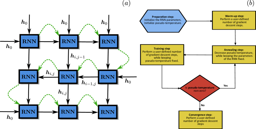
Here stands for the spins that were previously generated on the zigzag path as shown in Fig. 1(a). and are additional variational parameters. From the two previous relations, the probability and the phase can be computed respectively by taking the product (resp. sum) of (resp. ).
We note that to compute in the recursion relation (1), we use the neighbouring hidden states and spins, as demonstrated in Fig. 1(a). We also remark that a tensorized operation of the hidden states and the spins is chosen instead of a concatenation operation (see Eq. (1)) to improve the expressivity of the 2D RNN as shown in Ref. [24]. In this paper, we also use a gated version of the 2D RNN to further improve the accuracy of our 2D cRNN wave function ansatz. More details are shown in Appendix. A.
Furthermore, symmetries in a system of interest can be incorporated in RNN wave functions, namely symmetry and discrete lattice symmetries as it was shown in Ref. [1]. We highlight that adding symmetries significantly improves the accuracy of a variational calculation, as motivated in the literature with the example of RBM wave functions [25]. We finally emphasize that the variational parameters are optimized with the variational Monte Carlo (VMC) scheme to minimize where is the Hamiltonian describing a quantum system of interest. More details about this scheme can be found in the Appendix of Ref. [1].
2.2 Variational Annealing
Finding the ground state of a non-stoquastic Hamiltonian is limited by the sign problem [15, 16], and has shown to induce rugged landscapes during the VMC optimization [26]. The latter can make our ansatz stuck in a local minima, similarly to what is commonly observed in spin glass models at low temperatures. We take inspiration from the concept of annealing, where we supplement VMC with an artificial temperature to overcome local minima during a VMC optimization. This procedure has been already explored in Ref. [24] for the purpose of finding ground states of spin-glass models. Here, we explore this idea in the context of finding ground states of frustrated quantum systems.
In order to supplement the VMC scheme with annealing, we add a pseudo-entropy [14] on top of variational energy to obtain a variational free energy:
| (4) |
where is the von Neumann entropy, given by
| (5) |
Here the sum goes over all possible configurations . In this case is a pseudo-temperature. The latter is annealed starting from some initial temperature to zero temperature as follows: where and is the total number of annealing steps.
In our setup, we follow the same scheme in Ref. [24], where we first do training steps to prepare our RNN wave function close to the minimum of . In the second step, we keep the parameters of our ansatz fixed and we change to . In step 3, we perform gradient steps to bring the RNN ansatz closer to the minimum of . After iterating over steps 2 and 3, we arrive at . At this point, we perform a user-defined number of gradient steps to further improve our estimate of the ground state energy of . A flowchart detailing this procedure is provided in Fig. 1(b).
3 Results
We focus our attention on the task of finding the ground state of the two dimensional anti-ferromagnetic Heisenberg model on the square lattice and on the triangular lattice with open boundary conditions (OBC). The Hamiltonian is given as follows:
where the sum is over nearest neighbours and are Pauli matrices. In the square lattice case, has a symmetry111A point group with four rotations and four mirror reflections (vertical, horizontal and diagonal)., whereas for the case of the triangular lattice, has a symmetry222A point group with two rotations and two diagonal mirror reflections.. We also remark that in both cases, the ground state has zero magnetization [27], due to the symmetry of the Hamiltonian . We show that enforcing these symmetries in our ansatz allows to obtain a better accuracy without adding more parameters. More details about how to apply symmetries to the 2D cRNN ansatz can be found in the Appendix of Ref. [1].
3.1 Heisenberg model on the square lattice
Since the Hamiltonian can be made stoquastic on the sqaure lattice [28, 29], we set , i.e., we do not use annealing in this case. The latter choice is motivated by the observations shown in Appendix. B.
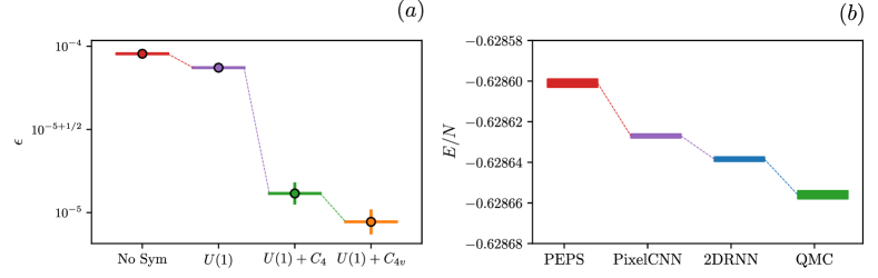
First, we train our 2D cRNN wave function to find the ground state of the square lattice with and without applying the symmetries of the Hamiltonian . We find in Fig. 2(a) that increasing the number of symmetries encoded in the cRNN leads to a more accurate estimation of the ground state energy.
We also use our 2D cRNN wave function to estimate the ground state of the square lattice after applying and symmetries. The results are shown in Fig. 2(b), where we compare our estimates with projected-pair entangled states (PEPS) [30], Pixel CNN wave functions [13], as well as Quantum Monte Carlo (QMC) [30]. These results show that our ansatz is more accurate compared to PEPS and PixelCNN. We also find that QMC is the best among all the three methods.
3.2 Heisenberg model on the triangular lattice
Due to the frustrated, non-bipartite nature of the triangular lattice, the Hamiltonian can no longer be made stoquastic with a simple unitary transformation. Such a Hamiltonian can make the VMC optimization landscape rough and filled with local minima [26]. Here, we use annealing to overcome local minima and to obtain accurate estimates of ground state energies.
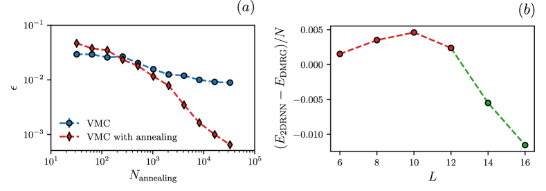
To demonstrate the idea of annealing, we target the ground state of the triangular lattice at different number of annealing steps . The results in Fig. 3(a) show that starting from a non-zero allows to obtain a lower value of the relative error as opposed to traditional VMC where the initial pseudo-temperature . We also remark that a higher accuracy is obtained by increasing the number of annealing steps, which underlines the importance of adiabaticity in our scheme.
We now focus our attention on larger system sizes. Here we train our 2D cRNN wave function using annealing for a system size . We then optimize our ansatz at larger system sizes after increasing the lattice side length by until we arrive at size . This step is done at zero pseudo-temperature and without reintializing the parameters of the RNN. This idea was already proposed in the literature in Ref. [14]. The latter takes advantage of the translation invariance property encoded in the weight-sharing of the parameters of the RNN (see Eqs. 1, 2 and 3). The results in Fig. 3(b) show that for system sizes larger than , the variational energy obtained by our RNN ansatz is more accurate compared to the energy obtained by DMRG. Interestingly, our RNN ansatz uses less than of the parameters of DMRG for system sizes larger than .
Conclusion
In this paper, we have applied a modified variant of the two dimensional RNN wave function [1, 24] for the task of finding the ground state of the 2D Heisenberg model on the square and the triangular lattice. We have shown that applying symmetry and annealing helps to obtain highly accurate ground states. We have also demonstrated the power of our ansatz compared to DMRG for large system size on the triangular lattice, where frustration makes the problem more challenging. We believe that more advanced versions of RNN wave functions along with the idea of applying symmetries and annealing can make our ansatz a highly competive tool for studying quantum many-body systems.
Note: the hyperparameters used to produce the results of this paper are detailed in Appendix. C.
Acknowledgments and Disclosure of Funding
Our RNN implementation is based on Tensorflow [31] and NumPy [32]. Computer simulations were made possible thanks to the Vector Institute computing cluster and the Compute Canada cluster. J.C. acknowledges support from Natural Sciences and Engineering Research Council of Canada (NSERC), the Shared Hierarchical Academic Research Computing Network (SHARCNET), Compute Canada, Google Quantum Research Award, and the Canadian Institute for Advanced Research (CIFAR) AI chair program. Research at Perimeter Institute is supported in part by the Government of Canada through the Department of Innovation, Science and Economic Development Canada and by the Province of Ontario through the Ministry of Economic Development, Job Creation and Trade.
Broader Impact
The scope of this paper is within quantum many-body physics, which aims to understand the behaviour of matter based on simple rules at the microscopic scale. In the best case, our method could enhance the state-of-the-art algorithms and enable a better understanding of unknown quantum systems.
Checklist
-
1.
For all authors…
-
(a)
Do the main claims made in the abstract and introduction accurately reflect the paper’s contributions and scope? [Yes]
-
(b)
Did you describe the limitations of your work? [Yes]
-
(c)
Did you discuss any potential negative societal impacts of your work? [N/A]
-
(d)
Have you read the ethics review guidelines and ensured that your paper conforms to them? [Yes]
-
(a)
-
2.
If you are including theoretical results…
-
(a)
Did you state the full set of assumptions of all theoretical results? [N/A]
-
(b)
Did you include complete proofs of all theoretical results? [N/A]
-
(a)
-
3.
If you ran experiments…
-
(a)
Did you include the code, data, and instructions needed to reproduce the main experimental results (either in the supplemental material or as a URL)? [Yes] Appendix. A provides more details about the 2DRNN cell we use in our study. We also provide more details in Appendix. C about the training process to facilitate the reproducibility of our results. Making our code publicly available is still a work in progress.
-
(b)
Did you specify all the training details (e.g., data splits, hyperparameters, how they were chosen)? [Yes] see Appendix. C.
-
(c)
Did you report error bars (e.g., with respect to the random seed after running experiments multiple times)? [Yes] the error bars correspond to a one standard deviation. They are computed after obtaining a large number of samples from the RNN using autoregressive sampling.
-
(d)
Did you include the total amount of compute and the type of resources used (e.g., type of GPUs, internal cluster, or cloud provider)? [Yes] We provide the type of GPUs we used to produce our results in Appendix. C. However, the total amount of compute was not included due to the lack of data.
-
(a)
-
4.
If you are using existing assets (e.g., code, data, models) or curating/releasing new assets…
-
(a)
If your work uses existing assets, did you cite the creators? [N/A]
-
(b)
Did you mention the license of the assets? [N/A]
-
(c)
Did you include any new assets either in the supplemental material or as a URL? [N/A]
-
(d)
Did you discuss whether and how consent was obtained from people whose data you’re using/curating? [N/A]
-
(e)
Did you discuss whether the data you are using/curating contains personally identifiable information or offensive content? [N/A]
-
(a)
-
5.
If you used crowdsourcing or conducted research with human subjects…
-
(a)
Did you include the full text of instructions given to participants and screenshots, if applicable? [N/A]
-
(b)
Did you describe any potential participant risks, with links to Institutional Review Board (IRB) approvals, if applicable? [N/A]
-
(c)
Did you include the estimated hourly wage paid to participants and the total amount spent on participant compensation? [N/A]
-
(a)
Appendix A Two dimensional gated recurrent neural networks
In this section, we show how we incorporate the gating mechanism in our 2D cRNN wave function ansatz. The 2D RNN cell we use is based on the following recursion relations:
| (6) | ||||
| (7) | ||||
| (8) |
Here we obtain the state through a combination of the neighbouring hidden states and the candidate hidden state . The update gate decides how much the candidate hidden state will be modified. The latter combination allows to circumvent some of the limitations related to the vanishing gradient problem [33, 34]. Note that the size of the hidden state that we denote as is a hyperparameter that we choose before optimizing the parameters of our ansatz. The tensors , the weight matrix and the biases are variational parameters of our RNN ansatz in addition to the parameters in Eqs. (2) and (3).
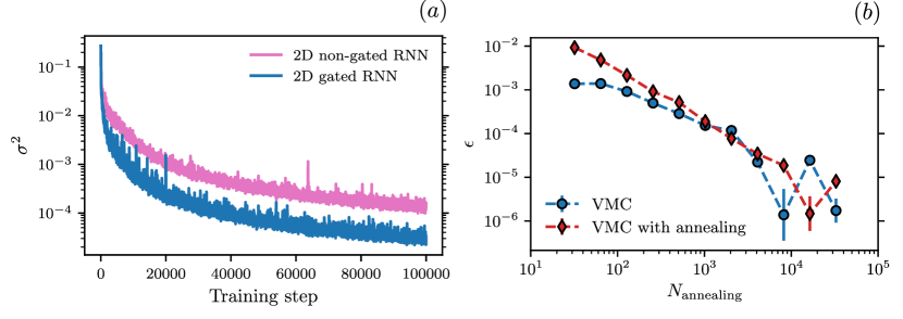
To show the advantage of a 2D gated RNN over the 2D non-gated RNN, we train them using the VMC scheme to find the ground state of the Heisenberg model on the square lattice with size . We find that the gated RNN allows to obtain a more accurate energy. More specifically, we plot the energy variance per spin in Fig. 4(a). This quantity is a good indicator for the proximity of the ansatz to the ground state provided that local minima are avoided [35, 36, 37]. We observe that the gated RNN can get about an order of magnitude lower compared to the non-gated RNN. The latter results demonstrate the advantage of adding the gating mechanism to our wave function ansatz.
Appendix B Annealing on the square lattice
In the results section, we have used on the square lattice which is equivalent to not doing annealing. This is motivated by the observation that the Heisenberg model on the square lattice is not frustrated and can made stoquastic using the Marshall sign rule [28, 29]. To further corroborate this observation, we compare VMC with and without annealing on the square lattice for a system size and report our results in Fig. 4(b). The latter illustrates that annealing does not show an advantage for large as opposed to the case of the triangular lattice demonstrated in Fig. 3(a). This result suggests that in the absence of frustration, there is no need to supplement VMC with annealing.
Appendix C Hyperparameters
| Figures | Parameter | Value |
| Fig. 2(a) | Architecture | 2D Tensorized Gated cRNN wave function |
| Number of memory units | ||
| Number of samples | ||
| Learning rate | ||
| Number of training steps | ||
| Fig. 2(b) | Architecture | 2D Tensorized Gated cRNN wave function |
| Number of memory units | ||
| Number of samples | ||
| Learning rate | ||
| Number of training steps | ||
| Applied symmetries | and | |
| Fig. 3(a) | Architecture | 2D Tensorized Gated cRNN wave function |
| Number of memory units | ||
| Number of samples | ||
| Learning rate | ||
| Number of warmup steps | ||
| Applied symmetries | and spin parity | |
| Fig. 4(a) | Number of memory units | |
| Number of samples | ||
| Learning rate | ||
| Applied symmetries | and | |
| Fig. 4(b) | Architecture | 2D Tensorized Gated cRNN wave function |
| Number of memory units | ||
| Number of samples | ||
| Learning rate | ||
| Number of warmup steps | ||
| Applied symmetries | and spin parity |
In this section, we summarize the hyperparameters used to produce the main results of this paper in Tab. 1. We note that the training of our ansatz was performed using P100 GPUs.
In order to produce the results of Fig. 3(b), we use and samples for training. We have first performed annealing on the system size with , , and an initial pseudo-temperature , while using a fixed learning rate . During each annealing step, we perform gradient descent steps. In this initial phase, we only apply the U(1) symmetry. In the next phase, we perform an additional gradients steps at zero pseudo-temperature and add an additional gradients steps after applying symmetry. During this convergence phase, the learning rate is decayed as , where corresponds to the current number of convergence steps. We then increase the system size to , while keeping our ansatz parameters fixed, applying symmetry and while using zero pseudo-temperature. In this phase, the learning rate is fixed to . After this step, we train our RNN ansatz until convergence. We repeat the same procedure for system sizes , , and . We note that for , we add gradient steps. For , we continue training with gradient steps. For , we converge using training steps. For , we continue training with gradient steps. Finally, for , we add convergence steps.
References
- Hibat-Allah et al. [2020] Mohamed Hibat-Allah, Martin Ganahl, Lauren E. Hayward, Roger G. Melko, and Juan Carrasquilla. Recurrent neural network wave functions. Physical Review Research, 2(2), Jun 2020. ISSN 2643-1564. doi: 10.1103/physrevresearch.2.023358. URL http://dx.doi.org/10.1103/PhysRevResearch.2.023358.
- Androsiuk et al. [1993] J. Androsiuk, L. Kulak, and K. Sienicki. Neural network solution of the Schrödinger equation for a two-dimensional harmonic oscillator. Chemical Physics, 173(3):377–383, 1993. ISSN 0301-0104. doi: 10.1016/0301-0104(93)80153-Z.
- LAG [1997] Artificial neural network methods in quantum mechanics. Computer Physics Communications, 104(1):1 – 14, 1997. ISSN 0010-4655. doi: https://doi.org/10.1016/S0010-4655(97)00054-4. URL http://www.sciencedirect.com/science/article/pii/S0010465597000544.
- Carrasquilla and Melko [2017] Juan Carrasquilla and Roger Melko. Machine learning phases of matter. Nature Physics, 14:431–434, 2017. doi: https://doi.org/10.1038/nphys4035.
- Carleo and Troyer [2017] Giuseppe Carleo and Matthias Troyer. Solving the quantum many-body problem with artificial neural networks. Science, 355(6325):602–606, Feb 2017. ISSN 1095-9203. doi: 10.1126/science.aag2302. URL http://dx.doi.org/10.1126/science.aag2302.
- Torlai et al. [2018] Giacomo Torlai, Guglielmo Mazzola, Juan Carrasquilla, Matthias Troyer, Roger Melko, and Giuseppe Carleo. Neural-network quantum state tomography. Nature Physics, 14:447–450, 2018. doi: https://doi.org/10.1038/s41567-018-0048-5.
- Carrasquilla et al. [2019] Juan Carrasquilla, Giacomo Torlai, Roger G. Melko, and Leandro Aolita. Reconstructing quantum states with generative models. Nature Machine Intelligence, 1(3):155–161, Mar 2019. ISSN 2522-5839. doi: 10.1038/s42256-019-0028-1. URL http://dx.doi.org/10.1038/s42256-019-0028-1.
- Cai and Liu [2018] Zi Cai and Jinguo Liu. Approximating quantum many-body wave functions using artificial neural networks. Phys. Rev. B, 97:035116, Jan 2018. doi: 10.1103/PhysRevB.97.035116. URL https://link.aps.org/doi/10.1103/PhysRevB.97.035116.
- Luo and Clark [2019] Di Luo and Bryan K. Clark. Backflow transformations via neural networks for quantum many-body wave functions. Phys. Rev. Lett., 122:226401, Jun 2019. doi: 10.1103/PhysRevLett.122.226401. URL https://link.aps.org/doi/10.1103/PhysRevLett.122.226401.
- Pfau et al. [2020] David Pfau, James S. Spencer, Alexander G. D. G. Matthews, and W. M. C. Foulkes. Ab initio solution of the many-electron schrödinger equation with deep neural networks. Physical Review Research, 2(3), Sep 2020. ISSN 2643-1564. doi: 10.1103/physrevresearch.2.033429. URL http://dx.doi.org/10.1103/PhysRevResearch.2.033429.
- Hermann et al. [2020] Jan Hermann, Zeno Schätzle, and Frank Noé. Deep-neural-network solution of the electronic schrödinger equation. Nature Chemistry, 12(10):891–897, Sep 2020. ISSN 1755-4349. doi: 10.1038/s41557-020-0544-y. URL http://dx.doi.org/10.1038/s41557-020-0544-y.
- Choo et al. [2020] Kenny Choo, Antonio Mezzacapo, and Giuseppe Carleo. Fermionic neural-network states for ab-initio electronic structure. Nature Communications, 11:2368, 2020. doi: https://doi.org/10.1038/s41467-020-15724-9.
- Sharir et al. [2020] Or Sharir, Yoav Levine, Noam Wies, Giuseppe Carleo, and Amnon Shashua. Deep autoregressive models for the efficient variational simulation of many-body quantum systems. Physical Review Letters, 124(2), Jan 2020. ISSN 1079-7114. doi: 10.1103/physrevlett.124.020503. URL http://dx.doi.org/10.1103/PhysRevLett.124.020503.
- Roth [2020] Christopher Roth. Iterative retraining of quantum spin models using recurrent neural networks, 2020.
- Troyer and Wiese [2005] Matthias Troyer and Uwe-Jens Wiese. Computational complexity and fundamental limitations to fermionic quantum monte carlo simulations. Physical Review Letters, 94(17), May 2005. ISSN 1079-7114. doi: 10.1103/physrevlett.94.170201. URL http://dx.doi.org/10.1103/PhysRevLett.94.170201.
- Westerhout et al. [2020] Tom Westerhout, Nikita Astrakhantsev, Konstantin S. Tikhonov, Mikhail I. Katsnelson, and Andrey A. Bagrov. Generalization properties of neural network approximations to frustrated magnet ground states. Nature Communications, 11(1):1593, March 2020. ISSN 2041-1723. doi: 10.1038/s41467-020-15402-w.
- Hochreiter and Schmidhuber [1997] Sepp Hochreiter and Jürgen Schmidhuber. Long short-term memory. Neural Comput., 9(8):1735–1780, November 1997. ISSN 0899-7667. doi: 10.1162/neco.1997.9.8.1735.
- Graves [2012] Alex Graves. Supervised sequence labelling. In Supervised sequence labelling with recurrent neural networks, pages 5–13. Springer, 2012. URL https://www.cs.toronto.edu/~graves/preprint.pdf.
- Lipton et al. [2015] Zachary C. Lipton, John Berkowitz, and Charles Elkan. A critical review of recurrent neural networks for sequence learning, 2015.
- Casert et al. [2020] Corneel Casert, Tom Vieijra, Stephen Whitelam, and Isaac Tamblyn. Dynamical large deviations of two-dimensional kinetically constrained models using a neural-network state ansatz, 2020.
- White [1992] Steven R. White. Density matrix formulation for quantum renormalization groups. Phys. Rev. Lett., 69:2863–2866, Nov 1992. doi: 10.1103/PhysRevLett.69.2863. URL https://link.aps.org/doi/10.1103/PhysRevLett.69.2863.
- Schollwöck [2005] U. Schollwöck. The density-matrix renormalization group. Reviews of Modern Physics, 77(1):259–315, Apr 2005. ISSN 1539-0756. doi: 10.1103/revmodphys.77.259. URL http://dx.doi.org/10.1103/RevModPhys.77.259.
- Bengio and Bengio [2000] S. Bengio and Y. Bengio. Taking on the curse of dimensionality in joint distributions using neural networks. IEEE Transactions on Neural Networks, 11(3):550–557, May 2000. ISSN 1045-9227. doi: 10.1109/72.846725.
- Hibat-Allah et al. [2021] Mohamed Hibat-Allah, Estelle M. Inack, Roeland Wiersema, Roger G. Melko, and Juan Carrasquilla. Variational neural annealing. Nature Machine Intelligence, October 2021. ISSN 2522-5839. doi: 10.1038/s42256-021-00401-3. URL https://doi.org/10.1038/s42256-021-00401-3.
- Nomura [2021] Yusuke Nomura. Helping restricted boltzmann machines with quantum-state representation by restoring symmetry. Journal of Physics: Condensed Matter, 33(17):174003, Apr 2021. ISSN 1361-648X. doi: 10.1088/1361-648x/abe268. URL http://dx.doi.org/10.1088/1361-648X/abe268.
- Bukov et al. [2021] Marin Bukov, Markus Schmitt, and Maxime Dupont. Learning the ground state of a non-stoquastic quantum hamiltonian in a rugged neural network landscape. SciPost Physics, 10(6), Jun 2021. ISSN 2542-4653. doi: 10.21468/scipostphys.10.6.147. URL http://dx.doi.org/10.21468/SciPostPhys.10.6.147.
- Lieb and Mattis [1962] Elliott Lieb and Daniel Mattis. Ordering energy levels of interacting spin systems. Journal of Mathematical Physics, 3(4):749–751, 1962. doi: 10.1063/1.1724276.
- Marshall [1955] W Marshall. Antiferromagnetism. Proceedings of the Royal Society of London. Series A. Mathematical and Physical Sciences, 232(1188):48–68, oct 1955. ISSN 2053-9169. doi: 10.1098/rspa.1955.0200. URL http://www.royalsocietypublishing.org/doi/10.1098/rspa.1955.0200.
- Capriotti [2001] Luca Capriotti. Quantum effects and broken symmetries in frustrated antiferromagnets. International Journal of Modern Physics B, 15(12):1799–1842, May 2001. ISSN 1793-6578. doi: 10.1142/s0217979201004605. URL http://dx.doi.org/10.1142/S0217979201004605.
- Liu et al. [2017] Wen-Yuan Liu, Shao-Jun Dong, Yong-Jian Han, Guang-Can Guo, and Lixin He. Gradient optimization of finite projected entangled pair states. Physical Review B, 95(19), May 2017. ISSN 2469-9969. doi: 10.1103/physrevb.95.195154. URL http://dx.doi.org/10.1103/PhysRevB.95.195154.
- Abadi et al. [2015] Martín Abadi, Ashish Agarwal, Paul Barham, Eugene Brevdo, Zhifeng Chen, Craig Citro, Greg S. Corrado, Andy Davis, Jeffrey Dean, Matthieu Devin, Sanjay Ghemawat, Ian Goodfellow, Andrew Harp, Geoffrey Irving, Michael Isard, Yangqing Jia, Rafal Jozefowicz, Lukasz Kaiser, Manjunath Kudlur, Josh Levenberg, Dandelion Mané, Rajat Monga, Sherry Moore, Derek Murray, Chris Olah, Mike Schuster, Jonathon Shlens, Benoit Steiner, Ilya Sutskever, Kunal Talwar, Paul Tucker, Vincent Vanhoucke, Vijay Vasudevan, Fernanda Viégas, Oriol Vinyals, Pete Warden, Martin Wattenberg, Martin Wicke, Yuan Yu, and Xiaoqiang Zheng. TensorFlow: Large-scale machine learning on heterogeneous systems, 2015. URL https://www.tensorflow.org/. Software available from tensorflow.org.
- Harris et al. [2020] Charles R. Harris, K. Jarrod Millman, Stéfan J. van der Walt, Ralf Gommers, Pauli Virtanen, David Cournapeau, Eric Wieser, Julian Taylor, Sebastian Berg, Nathaniel J. Smith, Robert Kern, Matti Picus, Stephan Hoyer, Marten H. van Kerkwijk, Matthew Brett, Allan Haldane, Jaime Fernández del Río, Mark Wiebe, Pearu Peterson, Pierre Gérard-Marchant, Kevin Sheppard, Tyler Reddy, Warren Weckesser, Hameer Abbasi, Christoph Gohlke, and Travis E. Oliphant. Array programming with numpy. Nature, 585(7825):357–362, Sep 2020. ISSN 1476-4687. doi: 10.1038/s41586-020-2649-2. URL https://doi.org/10.1038/s41586-020-2649-2.
- Zhou et al. [2016] Guo-Bing Zhou, Jianxin Wu, Chen-Lin Zhang, and Zhi-Hua Zhou. Minimal gated unit for recurrent neural networks, 2016.
- Shen [2019] Huitao Shen. Mutual information scaling and expressive power of sequence models, 2019.
- Gros [1990] Claudius Gros. Criterion for a good variational wave function. Phys. Rev. B, 42:6835–6838, Oct 1990. doi: 10.1103/PhysRevB.42.6835. URL https://link.aps.org/doi/10.1103/PhysRevB.42.6835.
- Assaraf and Caffarel [2003] Roland Assaraf and Michel Caffarel. Zero-variance zero-bias principle for observables in quantum monte carlo: Application to forces. The Journal of Chemical Physics, 119(20):10536–10552, 2003. doi: 10.1063/1.1621615. URL https://doi.org/10.1063/1.1621615.
- Becca and Sorella [2017] F. Becca and S. Sorella. Quantum Monte Carlo Approaches for Correlated Systems. Cambridge University Press, 2017. doi: 10.1017/9781316417041.
- Kingma and Ba [2017] Diederik P. Kingma and Jimmy Ba. Adam: A method for stochastic optimization, 2017.
- Fishman et al. [2020] Matthew Fishman, Steven R. White, and E. Miles Stoudenmire. The ITensor software library for tensor network calculations, 2020.