Searching for a Fifth Force with Atomic and Nuclear Clocks

Abstract

We consider the general class of theories in which there is a new ultralight scalar field that mediates an equivalence principle violating, long-range force. In such a framework, the sun and the earth act as sources of the scalar field, leading to potentially observable location dependent effects on atomic and nuclear spectra. We determine the sensitivity of current and next-generation atomic and nuclear clocks to these effects and compare the results against the existing laboratory and astrophysical constraints on equivalence principle violating fifth forces. We show that in the future, the annual modulation in the frequencies of atomic and nuclear clocks in the laboratory caused by the eccentricity of the earth’s orbit around the sun may offer the most sensitive probe of this general class of equivalence principle violating theories. Even greater sensitivity can be obtained by placing a precision clock in an eccentric orbit around the earth and searching for time variation in the frequency, as is done in anomalous redshift experiments. In particular, an anomalous redshift experiment based on current clock technology would already have a sensitivity to fifth forces that couple primarily to electrons at about the same level as the existing limits. Our study provides well-defined sensitivity targets to aim for when designing future versions of these experiments.

I Introduction

There are four known fundamental interactions in nature, namely gravity, electromagnetism, and the strong and weak nuclear forces. Taken together, these four forces provide an excellent fit to current experimental data. However, this need not be the complete picture and there may be additional interactions that have not yet been discovered, either because they are too weak or because their range is too short. The existence of such a fifth force constitutes one of the most intriguing possibilities for new physics beyond the Standard Model (SM) book ; Adelberger:2003zx .

String theory provides motivation for the existence of a long range fifth force. In this class of theories, the values of the fundamental constants are determined by the vacuum expectation values of scalar fields known as moduli. These scalar fields can have wildly varying masses, and some of them may be extremely light, see for example Damour:1994zq ; Damour:1994ya . In general, the couplings of moduli to matter need not respect the equivalence principle (EP). Therefore, such a field can serve as the mediator of a long range EP violating fifth force. Nonlinearly realized discrete symmetries can protect the mass of a modulus against radiative corrections even if it has sizable couplings to the SM fields Hook:2018jle ; Brzeminski:2020uhm . Apart from their contributions to fifth forces, moduli are a natural candidate for ultralight dark matter Turner:1983he ; Press:1989id ; Sin:1992bg . Many different types of searches have been proposed for this interesting class of dark matter candidates Khmelnitsky:2013lxt ; Stadnik:2014tta ; Arvanitaki:2015iga ; Graham:2015ouw ; Graham:2015ifn ; Stadnik:2015xbn ; Berlin:2016woy ; Geraci:2016fva ; Krnjaic:2017zlz ; Arvanitaki:2017nhi ; DeRocco:2018jwe ; Geraci:2018fax ; Irastorza:2018dyq ; Carney:2019cio ; Guo:2019ker ; Grote:2019uvn ; Dev:2020kgz .

There have been numerous experimental searches for new long range forces that violate the EP. Direct searches are based on comparing the motions of two bodies of different compositions in the gravitational field of a third. This class of searches includes experiments performed on suspended masses in the laboratory Braginskii:1971tn ; Schlamminger:2007ht ; Adelberger:2009zz ; Wagner:2012ui . It also includes observations of the motion of free-falling objects, such as test masses in the field of the earth Touboul:2017grn , the moon and earth in the gravitational field of the sun Dickey:1994zz ; Williams:2004qba , and gravitationally bound systems composed of three celestial bodies Ransom:2014xla ; Archibald:2018oxs . Searches have also been performed that use atom interferometry to compare the rates at which atoms of different materials fall in the earth’s gravitational field Fray:2004zs ; Zhou:2015pna ; Zhou:2019byc ; Schlippert:2014xla ; Tarallo:2014oaa . Although the limits from atom interferometry are not yet competitive with the results from experiments performed on macroscopic masses, major improvements are expected in the future Safronova:2017xyt ; MAGIS-100:2021etm . A broad review of precision tests of the EP, with many additional references, may be found in Ref. Tino:2020nla .

In this paper we explore a different approach to detecting long-range forces that violate the EP, based on the rapidly-improving sensitivity of atomic and nuclear clocks RevModPhys.87.637 ; McGrew:2018mqk ; PhysRevLett.120.103201 ; Bothwell_2019 . Using precision clock experiments to search for new physics is a rapidly growing field, see Ref. Safronova:2017xyt for a review. We limit our attention to the case when the fifth force is mediated by an ultralight scalar field. In general, the sun and the earth act as sources for any such scalar field. Then, since the values of fundamental parameters such as the fine structure constant $\alpha$ depend on the value of the scalar field, there are corrections to atomic and nuclear spectra that depend on the distance from these sources Flambaum:2007ar ; Shaw:2007ju ; Barrow:2008se . Atomic and nuclear clocks are sensitive to the frequencies of these transitions, and can therefore be used to search for position dependence of fundamental parameters. Since this effect is associated with EP violation Dent:2008gu ; Uzan:2010pm , this offers an alternative method of searching for EP violating fifth forces. Clock experiments also offer a new approach to detecting more exotic fifth forces such as chameleon models Khoury:2003aq ; Khoury:2003rn ; Feldman:2006wg ; Mota:2006ed that is distinct from the existing search methods Brax:2018iyo ; Sakstein:2018fwz ; Blinov:2018vgc .

Clock searches for EP violation are based on comparing two atomic or nuclear transition frequencies against each other. These frequencies could be those of two different clocks at the same physical location, or alternatively, two clocks at separate locations. In the case of two clocks at the same location, as long as their transition frequencies scale differently with fundamental parameters such as $\alpha$, the ratio of their frequencies will change as the distance from the source changes. For example, since the orbit of the earth around the sun is not a perfect circle, this results in an annual modulation in the frequencies of atomic and nuclear clocks Flambaum:2007ar ; Shaw:2007ju ; Barrow:2008se . We determine the sensitivities of current and next-generation atomic and nuclear clocks to this effect and compare the results against the existing laboratory and astrophysical constraints on EP violating fifth forces. We show that in the future, the annual modulation in the frequencies of atomic and nuclear clocks in the laboratory caused by the eccentricity of the earth’s orbit around the sun may offer the most sensitive probe of this general class of EP violating theories.

Even greater sensitivity can be obtained by comparing clocks at different locations. Comparing the frequency difference between a precision clock placed on a satellite in an eccentric orbit around the earth and a similar clock on earth would offer an extremely sensitive probe of this class of models. Experiments of this type have already been performed to test the general relativistic prediction for the gravitational redshift Gravity_Probe_A ; Delva:2018ilu , and new ones proposed Derevianko:2021kye ; Tsai:2021lly ; Schkolnik:2022utn . Importantly, we find that such an experiment that employs current clock technology would already have a sensitivity to fifth forces that couple primarily to electrons at the about the same level as the existing limits. The reason for this is that direct fifth force searches are inherently less sensitive to forces acting on electrons, since electrons comprise less than 0.1% of the mass of an atom. In contrast, atomic transition frequencies are extremely sensitive to the properties of the electron. Our analysis provides well-defined sensitivity targets to aim for when designing future versions of these experiments.

The outline of this paper is as follows. In the next section we consider the interactions of an ultralight scalar with the SM and discuss the current constraints on this framework from direct searches for EP violation and from recasting existing clock experiments. In Section III we study the sensitivity of next-generation atomic and nuclear clocks to this class of models, and show that they can explore new parameter space. We conclude in Section IV.

II Ultralight Scalar Fields and Equivalence Principle Violation

In this section, we present a general framework for studying the effects of an ultralight scalar coupled to the SM. We show how direct fifth force, gravitational redshift, and differential redshift measurements can be used to place bounds on the parameters in the Lagrangian. This allows a concrete comparison of the sensitivities of these different experiments.

Consider an ultralight light scalar field $\phi$ that couples to the particles in the SM. At energies well below the weak scale, the interactions of $\phi$ with the stable matter fields and the light force carriers of the SM can be conveniently parametrized as Damour2010_convention ; Damour:2010rm

$$\mathcal{L}\supset\kappa\phi\Big{[}\frac{d_{e}}{4e^{2}}F_{\mu\nu}F^{\mu\nu}-\frac{d_{g}\beta_{3}}{2g_{3}}G^{A}_{\mu\nu}G^{A\mu\nu}-d_{m_{e}}m_{e}\bar{\psi}_{e}\psi_{e}\\ -\sum_{i=u,d}{(d_{m_{i}}+\gamma_{m_{i}}d_{g})m_{i}\bar{\psi}_{i}\psi_{i}}\Big{]}\;.$$ (1)

Here the parameter $\kappa$ is defined as $\kappa=\sqrt{4\pi G}$, where $G$ is Newton’s constant. This parametrization allows a straightforward comparison between the force mediated by the ultralight scalar and gravitational effects. In this expression $e$ represents the charge of the electron, $g_{3}$ the coupling constant of quantum chromodynamics (QCD) and $\beta_{3}\equiv\partial g_{3}/\partial\log\mu$ its beta function. The parameters $m_{i}$ denote the masses of the fermions and $\gamma_{m}\equiv-\partial\log m/\partial\log\mu$. The parameters $d_{x}$ with $x\in\{e,g,m_{i}\}$ represent the couplings of the scalar to the corresponding gauge bosons and fermions. The couplings of the scalar have been parametrized such that the limit $d_{g}=d_{m_{e}}=d_{m_{i}}$ with $d_{e}=0$ corresponds to the interactions of a dilaton that respects the equivalence principle. At these energies the SM has an approximate parity symmetry under which $\phi$ has been taken to be even. This represents the most general form of the interaction consistent with the symmetries up to terms of dimension 5 and linear order in $\phi$. In order to isolate the EP violating effects, it is conventional to parameterize the Lagrangian in Eq. (1) in terms of the average light quark mass $\hat{m}\equiv(m_{u}+m_{d})/2$ and the mass difference $\delta m\equiv(m_{d}-m_{u})$ rather than the light quark masses $m_{u}$ and $m_{d}$. The corresponding couplings of the modulus take the form,

$$\mathcal{L}\supset-\kappa\phi\left[d_{\hat{m}}\hat{m}(\bar{d}d+\bar{u}u)+\frac{d_{\delta m}}{2}\delta m(\bar{d}d-\bar{u}u)\right],$$ (2)

where

$$d_{\hat{m}} =\frac{d_{m_{d}}m_{d}+d_{m_{u}}m_{u}}{m_{d}+m_{u}}$$

$$d_{\delta m} =\frac{d_{m_{d}}m_{d}-d_{m_{u}}m_{u}}{m_{d}-m_{u}}.$$ (3)

As a result of the interactions in Eq. (1), the scalar field gives rise to a force between any two macroscopic bodies Damour:2010rm . By convention, this new force is parametrized in terms of its strength relative to the gravitational force. Accordingly, the potential energy $V$, which includes the effects of both the gravitational force and the new force, now takes the form,

$$V=-G\frac{m_{\bf A}m_{\bf B}}{r_{\bf AB}}(1+\alpha_{\bf A}\alpha_{\bf B}e^{-\frac{r_{\bf AB}}{\lambda}})\;.$$ (4)

Here $m_{\bf A}$ and $m_{\bf B}$ are the masses of the two bodies A and B, $r_{\bf AB}$ is the distance between them, and $\lambda\equiv 1/m_{\phi}$ sets the range of the interaction. The parameters $\alpha_{\bf A}$ and $\alpha_{\bf B}$, which are functions of $d_{e}$, $d_{g}$, $d_{m_{e}}$ and $d_{m_{i}}$, depend on the compositions of A and B. Therefore, in general, the force mediated by $\phi$ violates the EP. The parameters $\alpha_{\bf A}$ and $\alpha_{\bf B}$ can be approximated as,

$$\alpha_{\bf X}\simeq d_{g}^{*}+ \left[(d_{\hat{m}}-d_{g})Q_{\hat{m}}+(d_{\delta m}-d_{g})Q_{\delta m}+(d_{m_{e}}-d_{g})Q_{m_{e}}\right.$$ (5)

$$+\left.d_{e}Q_{e}\right]_{\bf X}\;,$$

where the composition-independent part $d_{g}^{*}$ is given by

$$d_{g}^{*}\equiv d_{g}+0.093(d_{\hat{m}}-d_{g})+10^{-4}[2.7d_{e}+2.75(d_{m_{e}}-d_{g})].$$ (6)

The remaining composition-dependent part of $\alpha_{\mathbf{X}}$ in Eq. (5) is parameterized in terms of the variables $Q_{\hat{m}}$, $Q_{\delta m}$, $Q_{e}$ and $Q_{m_{e}}$ that depend on the mass number $A$ and atomic number $Z$ of the atomic nuclei of which the body is composed,

$$Q_{\hat{m}} \equiv-\frac{0.036}{A^{1/3}}-1.4\times 10^{-4}\frac{Z(Z-1)}{A^{4/3}}-0.02\frac{(A-2Z)^{2}}{A^{2}},$$ (7)

$$Q_{\delta m} \equiv 1.7\times 10^{-3}\frac{A-2Z}{A},$$

$$Q_{e} \equiv 7.7\times 10^{-4}\frac{Z(Z-1)}{A^{4/3}}+8.2\times 10^{-4}\left(\frac{Z}{A}-\frac{1}{2}\right),$$

$$Q_{m_{e}} \equiv 5.5\times 10^{-4}\left(\frac{Z}{A}-\frac{1}{2}\right).$$

We see from this that $\alpha_{\bf X}$ naturally splits up into a composition-independent term $d_{g}^{*}$ and a composition-dependent term that is contained in the square bracket in Eq. (5). For a general choice of modulus couplings the term in the square brackets does not vanish, so the contribution to the potential from the ultralight scalar depends on the compositions of the test bodies. Therefore the resulting force violates the weak EP. The existing limits on EP violating forces can be translated into bounds on the couplings of the scalar $\phi$.

We see from Eq. (7) that $|Q_{\delta m}|\ll|Q_{\hat{m}}|$. We therefore expect that, in general, experiments searching for EP violation will be much more sensitive to the coupling $d_{\hat{m}}$ than to $d_{\delta m}$. For simplicity, we will therefore neglect the coupling $d_{\delta m}$ in the discussion that follows.

Apart from generating an EP violating force, the interactions in Eq. (1) imply that the effective values of fundamental constants such as $\alpha$ and $m_{e}$ at any given location depend on the value of $\phi$ at that location. For example, for these two parameters we have,

$$\alpha(x)=\bar{\alpha}[1+d_{e}\kappa\phi(x)]\quad m_{e}(x)=\bar{m_{e}}[1+d_{m_{e}}\kappa\phi(x)]\;.$$ (8)

Here $\bar{\alpha}$ ($\bar{m_{e}}$) denotes the value of the fine structure constant (electron mass) in the absence of the terms in Eq. (1). Consequently the sourcing of $\phi$ by massive objects such as the sun and the earth causes the value of fundamental constants such as $\alpha$ and $m_{e}$ to depend on the distance from these sources. This offers an alternative method of probing this class of models using atomic and nuclear clocks, which is the focus of this paper.

II.1 Direct Fifth Force Measurements

In this subsection we review how to map the limits from direct fifth force searches onto bounds on the parameters in Eq. (1). The results are summarized in Eqs. (12), (13), (14) and (15).

At present, the most precise tests of EP violation are based on measurements of how two test bodies A and B composed of different materials accelerate towards a third body C, which is usually the earth or the sun. If the EP holds, the two accelerations should be identical. By convention, the experimental limits on EP violation are expressed in terms of the Eotvos parameter,

$$\eta\equiv 2\frac{|\vec{a}_{\bf A}-\vec{a}_{\bf B}|}{|\vec{a}_{\bf A}+\vec{a}_{\bf B}|}$$ (9)

where $a_{\bf A}$ and $a_{\bf B}$ represent the accelerations of the test bodies A and B. Since the interactions in Eq. (1) give rise to an EP violating force between any two macroscopic bodies, the experimental limits on $\eta$ can be translated into bounds on the couplings of the ultralight scalar to matter.

In the limit that the distances between the bodies A,B and C are all much smaller than $\lambda$, so that the mass of the modulus can be neglected, we can estimate the Eotvos parameter in this class of models from Eq. (4) as,

$$\eta \approx(\alpha_{\bf A}-\alpha_{\bf B})\alpha_{\bf C}$$ (10)

$$\approx\left[\Delta Q_{\hat{m}}(d_{\hat{m}}-d_{g})+\Delta Q_{e}d_{e}+\Delta Q_{m_{e}}(d_{m_{e}}-d_{g})\right]\alpha_{\bf C}\;.$$

In most simple models the composition independent part of $\alpha_{\bf C}$ will dominate over composition dependent part. In this case we can make the approximation $\alpha_{\bf C}\approx d_{g}^{*}$ so that

$$\eta \approx\left[\Delta Q_{\hat{m}}(d_{\hat{m}}-d_{g})+\Delta Q_{e}d_{e}+\Delta Q_{m_{e}}(d_{m_{e}}-d_{g})\right]d_{g}^{*}$$ (11)

$$\approx\Delta Q_{\hat{m}}D_{\hat{m}}+\Delta Q_{e}D_{e}+\Delta Q_{m_{e}}D_{m_{e}}\;.$$

Here we have defined $D_{e}\equiv d^{*}_{g}d_{e}$, $D_{\hat{m}}\equiv d^{*}_{g}(d_{\hat{m}}-d_{g})$ and $D_{m_{e}}\equiv d^{*}_{g}(d_{m_{e}}-d_{g})$. Since typically $\Delta Q_{m_{e}}\ll\Delta Q_{e}\,,\Delta Q_{\hat{m}}$, using the experimental bound on $\eta$ for two given test bodies of known compositions, the allowed $(D_{\hat{m}},D_{e})$ parameter space can be constrained to a band as shown in Fig. 1. The most accurate measurement of $\eta$, performed by the MICROSCOPE mission Touboul:2017grn ; Berge2017_MICROSCOPE , sets constraints at the $10^{-14}$ level and is represented by the black band in Fig. 1.

Figure 1: Current bounds on $D_{e}$ vs. $D_{\hat{m}}$ set by fifth force experiments Wagner:2012ui ; Touboul:2017grn ; Berge2017_MICROSCOPE ; Braginskii:1971tn . The black band represents the bound set by MICROSCOPE Berge2017_MICROSCOPE ; Touboul:2017grn , the blue and yellow bands are the constraints set by the EotWash group with Be-Ti and Be-Al masses Wagner:2012ui , and the green band is the Moscow group’s result obtained with Al-Pt masses Braginskii:1971tn .

In addition to constraining the $D_{\hat{m}}$ and $D_{e}$ parameters, we can translate the bounds on the Eotvos parameter $\eta$ into limits on the individual modulus couplings $d_{x}$. For example, using Eq. (10) we can set an upper bound on $d_{g}$ assuming that all the other couplings vanish,

$$\eta\approx\Delta Q_{\hat{m}}d_{g}^{2}\;\;\;\Rightarrow\;\;\;d_{g}=\sqrt{\frac{\eta}{\Delta Q_{\hat{m}}}}\;,d_{\hat{m}}=d_{m_{e}}=d_{e}=0.$$ (12)

The analogous bounds on $d_{e}$, $d_{\hat{m}}$ and $d_{m_{e}}$ are given by,

$$d_{e}=\sqrt{\frac{\eta}{\Delta Q_{e}(2.7\times 10^{-4}+Q_{e,\bf C})}}\;,\;d_{\hat{m}}=d_{m_{e}}=d_{g}=0,$$ (13)

$$d_{\hat{m}}=\sqrt{\frac{\eta}{\Delta Q_{\hat{m}}(9.3\times 10^{-2}+Q_{\hat{m},\bf C})}}\;,\;d_{m_{e}}=d_{e}=d_{g}=0,$$ (14)

$$d_{m_{e}}=\sqrt{\frac{\eta}{\Delta Q_{m_{e}}(2.75\times 10^{-4}+Q_{m_{e},\bf C})}}\;,\;d_{\hat{m}}=d_{e}=d_{g}=0.$$ (15)

By performing multiple measurements on bodies of different compositions, it is in principle possible to set independent constraints on all of the $D_{x}$ and $d_{x}$ parameters.

Although these bounds have been obtained under the assumption that the distances between the bodies A, B and C are all much smaller than $\lambda$, the extension of these limits to the more general case is straightforward Adelberger:2003zx ; Berge2017_MICROSCOPE ,

$$d_{x}=\frac{d_{x}^{\text{massless}}}{\sqrt{\Phi(\frac{R_{\bf C}}{\lambda})(1+\frac{r}{\lambda})e^{-\frac{r}{\lambda}}}}\;.$$ (16)

Here $\Phi(x)\equiv 3(x\cosh{x}-\sinh{x})/x^{3}$, $R_{\bf C}$ is the radius of the body C, and $d_{x}^{\text{massless}}$ represents the corresponding bound in the limit that $m_{\phi}=0$, given by Eqs. (12), (13), (14) and (15).

II.2 Clock Experiments

In this subsection, we show how to map the results of clock experiments onto the parameter space shown in Eq. (1). This allows for a direct comparison between clock experiments and direct fifth force measurements.

While direct measurement of the fifth force currently provides the most stringent constraints on the couplings $d_{x}$ of the ultralight scalar, there is an alternative method to constrain the new force. Recall that the couplings introduced in Eq. (1) modify the potential energy between two masses as shown in Eq. (4). The correction to the potential energy can be rewritten in the familiar form,

$$\delta V=-G\frac{m_{\bf A}m_{\bf B}}{r_{\bf AB}}\alpha_{\bf A}\alpha_{\bf B}e^{-\frac{r_{\bf AB}}{\lambda}}=-\frac{q_{\bf A}q_{\bf B}}{4\pi r_{\bf AB}}e^{-\frac{r_{\bf AB}}{\lambda}}\;,$$ (17)

where $q_{\bf X}=\kappa\alpha_{\bf X}m_{\bf X}$ represents the charge of the body under the new Yukawa force. From the above expression we see that each massive body X sources the scalar field $\phi$ as,

$$\phi_{\bf X}=-\frac{q_{\bf X}}{4\pi r}e^{-\frac{r}{\lambda}}.$$ (18)

As can be seen from Eq. (8), the scalar field $\phi$ affects the values of fundamental constants. This results in a spatial variation in the values of fundamental constants in the vicinity of a source body X. For example, in the case of the fine structure constant we have,

$$\frac{\Delta\alpha}{\alpha}=d_{e}\kappa\phi_{\bf X}=-\frac{d_{e}\alpha_{\bf X}Gm_{\bf X}}{r}e^{-\frac{r}{\lambda}}=d_{e}\alpha_{\bf X}U_{\bf X}e^{-\frac{r}{\lambda}}\;.$$ (19)

Here $U_{\bf X}$ represents the gravitational potential sourced by the body X. From the above equation, we see that measuring the variation of fundamental constants in the neighborhood of a massive body such as the earth or sun allows us to probe the same couplings that direct fifth force searches are sensitive to. We now discuss the sensitivity of atomic and nuclear clocks to this variation.

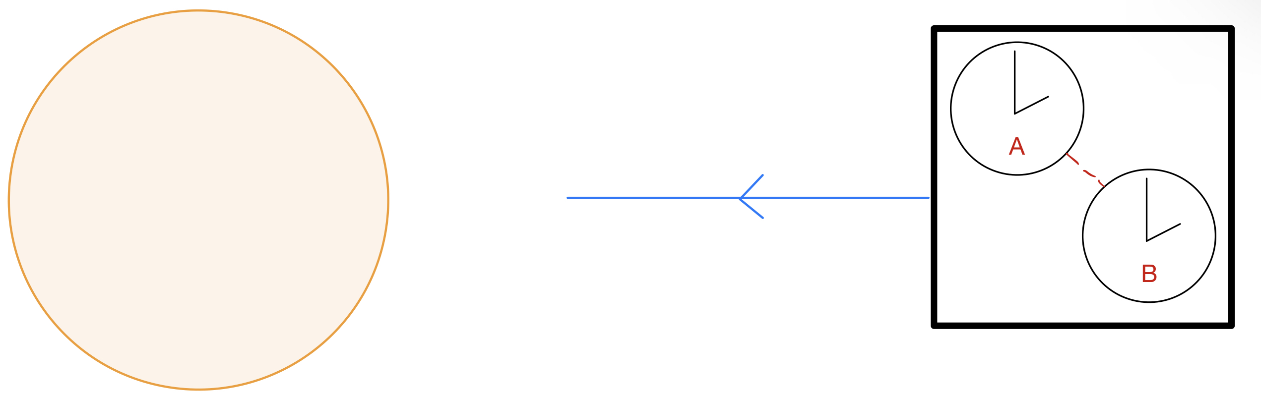
Figure 2: A schematic picture of an experiment involving two different clocks that travel together and experience the same change in the gravitational potential. The location dependence of the ratio of the two transition frequencies is a sensitive probe of EP violation.

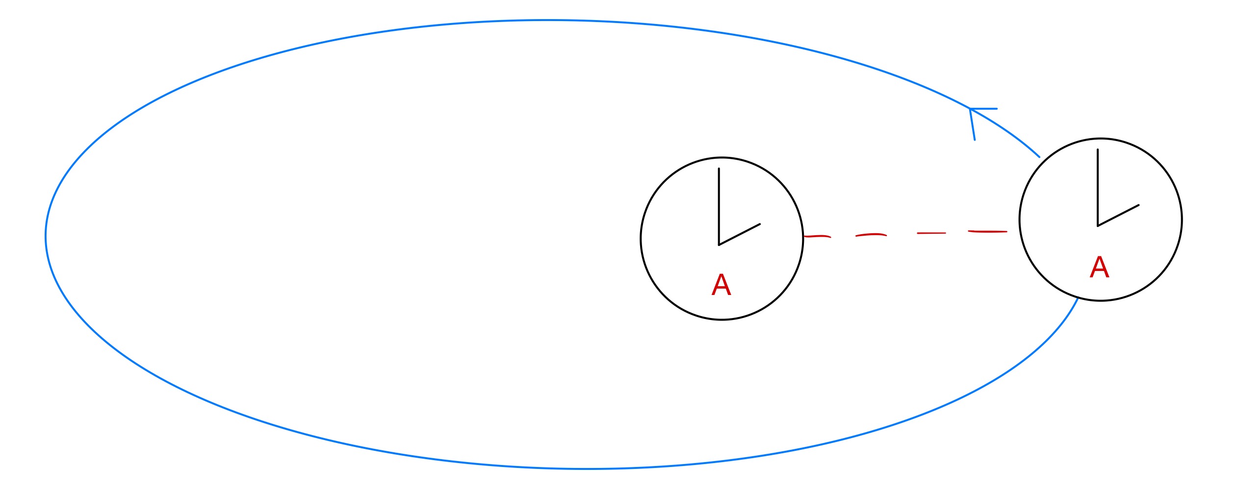
Figure 3: A schematic picture of an experiment involving two identical clocks that are spatially separated. The dependence of the difference in frequencies between the two clocks on the difference in the gravitational potential between their locations is a sensitive probe of EP violation.

The principle of Local Position Invariance (LPI) states that the frequency of any given clock in its local frame is independent of its position in space. This can be expressed as

$$f^{local}_{A}(x)=f^{local}_{A}(\infty),$$ (20)

where $f^{local}_{A}(\infty)$ denotes the frequency of the clock A at infinity, where the gravitational potential $U$ vanishes. It follows from Eq. (19) that in the class of theories we are considering the values of the fundamental constants are not the same at different points in space. Then the frequencies of clocks depend on their location in space and so the principle of LPI is no longer valid. Therefore Eq. (20) will receive corrections whose magnitude will, in general, depend on the type of the clock used in the experiment. This violation of LPI can be parametrized in terms of the anomalous redshift parameter $\beta_{A}$ as

$$\frac{f^{local}_{A}(x)-f^{local}_{A}(\infty)}{f^{local}_{A}(\infty)}=\beta_{A}U(x)\;,$$ (21)

where values of $\beta_{A}$ different from zero are the result of new physics. The subscript $A$ indicates the type of clock being employed. In practice, when comparing two clocks, one typically measures frequencies in the rest frame of one of the clocks, which we identify with the lab frame. This leads to the relation 

$$\frac{f^{\text{lab}}_{A}(x)-f^{\text{lab}}_{A}(x_{\text{lab}})}{f^{\text{lab}}_{A}(x_{\text{lab}})}=(1+\beta_{A})[U(x)-U(x_{\text{lab}})]\;.$$ (22)

Here the term $1$ in the bracket represents the standard prediction from general relativity and $x_{\text{lab}}$ denotes the position of the lab.

The dependence of a clock transition on fundamental parameters is conventionally expressed as

$$f_{A}\propto R\,\alpha^{K^{A}_{\alpha}}\mu^{K^{A}_{\mu}}X_{q}^{K^{A}_{q}}\propto m_{e}\,\alpha^{K^{A}_{\alpha}+2}\mu^{K^{A}_{\mu}}X_{q}^{K^{A}_{q}},$$ (23)

where $\alpha$ is the fine structure constant, $\mu\equiv{m_{p}}/{m_{e}}$ is the proton-to-electron mass ratio, $X_{q}\equiv{m_{q}}/{\Lambda_{QCD}}$ is the ratio of the average light quark mass to the QCD scale and $R\propto m_{e}\alpha^{2}$ denotes the Rydberg constant. The coefficients $K^{A}_{\alpha,\mu,q}$ characterize the sensitivity of a given transition to variations of the corresponding parameters. Typically, $K^{A}_{\mu}=-1$ for hyperfine transitions, $K^{A}_{\mu}=0$ for optical and $K^{A}_{\mu}=1$ for nuclear transitions. The $K^{A}_{\alpha,q}$ have to be determined numerically for each transition.

From Eqs. (21) and (23) we find

$$\beta_{A}U(x)=\frac{\Delta m_{e}}{m_{e}}+(K^{A}_{\alpha}+2)\frac{\Delta\alpha}{\alpha}+K^{A}_{\mu}\frac{\Delta\mu}{\mu}+K^{A}_{q}\frac{\Delta X_{q}}{X_{q}}\;,$$ (24)

where $\frac{\Delta X}{X}=\frac{X(x)-X(\infty)}{X(\infty)}$ with $X\in\{\alpha,\mu,X_{q},m_{e}\}$. Using this equation, constraints on $\beta_{A}$ can be turned into bounds on the variation of various fundamental constants.

In order to compare these bounds with those from fifth force experiments we need to express the variation of the fundamental parameters in terms of the couplings shown in Eq. (1). A brief calculation yields

$$\frac{\Delta\alpha}{\alpha} =d_{e}\alpha_{\bf X}U\simeq D_{e}U,$$ (25)

$$\frac{\Delta\mu}{\mu} =-(d_{m_{e}}-d_{g})\alpha_{\bf X}U\simeq-D_{m_{e}}U,$$

$$\frac{\Delta X_{q}}{X_{q}} =(d_{\hat{m}}-d_{g})\alpha_{\bf X}U\simeq D_{\hat{m}}U,$$

$$\frac{\Delta m_{e}}{m_{e}} =d_{m_{e}}\alpha_{\bf X}U\simeq(D_{m_{e}}+D_{g})U\;,$$

where in the second step we have approximated $\alpha_{\bf X}\approx d_{g}^{*}$ and defined $D_{g}\equiv d_{g}d_{g}^{*}$. These expressions are valid for $r\ll\lambda$. Experiments that constrain the variation of fundamental constants sometimes employ the alternative parameterization, ${\Delta X}/{X}=k_{X}U$. From Eq. (25), we see that $k_{\alpha}=D_{e}$, $k_{\mu}=-D_{m_{e}}$, and $k_{q}=D_{\hat{m}}$. The translation of bounds between the two different parametrizations is therefore straightforward.

From Eqs. (24) and (25) we can express $\beta_{A}$ in terms of the couplings of the modulus,

$$\beta_{A} =\left[(K^{A}_{\alpha}+2)d_{e}-K^{A}_{\mu}(d_{m_{e}}-d_{g})+K^{A}_{q}(d_{\hat{m}}-d_{g})+d_{m_{e}}\right]\alpha_{\bf X}$$ (26)

$$\approx(K^{A}_{\alpha}+2)D_{e}+(1-K^{A}_{\mu})D_{m_{e}}+K^{A}_{q}D_{\hat{m}}+D_{g}\;.$$

Since direct fifth force measurements are also sensitive to the $D_{x}$, the relation above allows for a direct comparison between these experiments and clock experiments.

We can translate the bounds on $\beta_{A}$ into bounds on the modulus couplings $d_{x}$ under the assumption that only one coupling has a non-zero value,

$$d_{g}=\sqrt{\frac{\beta_{A}}{|K_{\mu}^{A}-K_{q}^{A}|}}\;,\;d_{\hat{m}}=d_{e}=d_{m_{e}}=0,$$ (27)

$$d_{e}=\sqrt{\frac{\beta_{A}}{|K_{\alpha}^{A}+2|(2.7\times 10^{-4}+Q_{e,X})}}\;,\;d_{\hat{m}}=d_{g}=d_{m_{e}}=0,$$ (28)

$$d_{\hat{m}}=\sqrt{\frac{\beta_{A}}{|K_{q}^{A}|(9.3\times 10^{-2}+Q_{\hat{m},X})}}\;,\;d_{e}=d_{g}=d_{m_{e}}=0.$$ (29)

$$d_{m_{e}}=\sqrt{\frac{\beta_{A}}{|1-K_{\mu}^{A}|\,(2.75\times 10^{-4}+Q_{m_{e},X})}}\;,\;d_{e}=d_{g}=d_{\hat{m}}=0.$$ (30)

By employing multiple clocks, each of a different composition, it is in principle possible to set independent constraints on all of the $D_{x}$ and $d_{x}$ parameters.

Our results have been derived under the assumption that the experiments were performed at distances such that $r\ll\lambda$. When we relax this assumption, the above formulas generalize to Adelberger:2003zx

$$d_{x}=\frac{d_{x}^{\text{massless}}}{\sqrt{\Phi(\frac{R_{\bm{X}}}{\lambda})e^{-\frac{r}{\lambda}}}},$$ (31)

where $d_{x}^{\text{massless}}$ is the corresponding parameter given in Eqs. (27), (28), (29) and (30).

The clock experiments that search for fifth forces fall into two distinct classes, differential redshift measurements and gravitational redshift measurements, illustrated in Figs. 3 and 3 respectively. Differential redshift measurements involve comparing two clocks composed of different materials at the same location as they orbit another body. Gravitational redshift measurements involve comparing the frequencies of a clock in orbit around the earth with a clock on earth. This class of experiments is sensitive to the redshift predicted by general relativity and bounds are placed on any additional source of redshift. We now consider the existing limits from these two classes of experiments in turn.

We first consider differential redshift measurements. A comparison of two different clocks $A$ and $B$ that experience the same change in the potential allows a measurement of the difference $(\beta_{A}-\beta_{B})$. Then, using Eq. (26), we can easily recover information about the couplings of the modulus,

$$\beta_{AB} =[\Delta K^{AB}_{\alpha}d_{e}-\Delta K^{AB}_{\mu}(d_{m_{e}}-d_{g})+\Delta K^{AB}_{q}(d_{\hat{m}}-d_{g})]\alpha_{\bf X}$$ (32)

$$\approx\Delta K^{AB}_{\alpha}D_{e}-\Delta K^{AB}_{\mu}D_{m_{e}}+\Delta K^{AB}_{q}D_{\hat{m}}\;.$$

Here we have defined, $\beta_{AB}\equiv\beta_{A}-\beta_{B}$ and $\Delta K^{AB}_{X}\equiv K^{A}_{X}-K^{B}_{X}$.

A natural realization of the experiment involves comparing the frequencies of two different clocks in the laboratory over the course of a year PhysRevLett.111.060801 ; Leefer:2016xfu ; Lange:2020cul . As the distance between earth and the sun changes due to the eccentricity of the orbit, the frequencies of the clocks change accordingly. The ratio of the frequencies of the two clocks, $\tilde{f}(x)\equiv f^{local}_{A}(x)/f^{local}_{B}(x)$ changes as

$$\frac{\tilde{f}(x(t))-\tilde{f}(x(t_{0}))}{\tilde{f}(x(t_{0}))}=(\beta_{A}-\beta_{B})\left[U(x(t))-U(x(t_{0}))\right]\;.$$ (33)

Therefore, by comparing the frequencies of the clocks over the course of a year, we can obtain a measurement of $(\beta_{A}-\beta_{B})$. Currently, state-of-the-art experiments constrain this ratio at the $10^{-7}$ level Lange:2020cul , which results in the following limits,

$$D_{e}\lesssim 10^{-8},\quad D_{m_{e}}\lesssim 10^{-6},\quad D_{\hat{m}}\lesssim 10^{-6}\;.$$ (34)

From Fig. 1, we see that the limits from this class of atomic clock experiments are currently at least 3 orders of magnitude weaker than the direct limits from fifth force measurements in the $(D_{e},D_{\hat{m}})$ parameter space.

We now turn our attention to gravitational redshift measurements. As Eq. (22) suggests, $\beta_{A}$ can be determined by comparing two identical spatially separated clocks, as illustrated in Fig. 3. This approach is also not new. The first successful realization of this method was achieved by Gravity Probe - A Gravity_Probe_A , where the frequency of a microwave clock on a satellite was compared with the frequency of an identical clock on earth via microwave link as the satellite was changing altitude. After accounting for special and general relativistic effects, the measured frequency was transformed to the local frame of satellite leading to a constraint on the anomalous redshift via the relation,

$$\frac{f^{local}_{A}(x)-f^{local}_{A}(x_{\oplus})}{f^{local}_{A}(x_{\oplus})}=\beta_{A}\left[U(x)-U(x_{\oplus})\right],$$ (35)

where $x_{\oplus}$ denotes the position of the clock on earth.

This experiment constrained $\beta_{A}$ at the level of $10^{-4}$. Although this bound was later improved by an order of magnitude by the Galileo satellite Delva:2018ilu , it remains many orders of magnitude below the strongest limits from direct fifth force searches.

III Experimental prospects

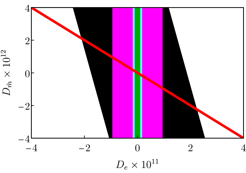
Figure 4: In the $D_{\hat{m}}$ vs. $D_{e}$ plane, we show how the projected limits from future earth and space based differential redshift experiments compare against the current bounds from direct fifth force searches. The black region represents the current bound set by MICROSCOPE Touboul:2017grn ; Berge2017_MICROSCOPE . The magenta and light cyan lines show the projected sensitivity of the SpaceQ experiment Tsai:2021lly while traveling towards the $r=0.39$ AU and $r=0.1$ AU orbits respectively, assuming that the satellite is equipped with two optical clocks with $\Delta K_{\alpha}=7$ and ${\Delta\tilde{f}}/{\tilde{f}}=10^{-18}$. The green band shows the projected sensitivity of an earth based experiment based on two optical clocks with $\Delta K_{\alpha}=7$, $\Delta K_{q}=0$ and ${\Delta\tilde{f}}/{\tilde{f}}=10^{-21}$. The red line shows the bound that could be set by an earth based nuclear clock - optical clock system, with $\Delta K_{\alpha}=10^{4}$, $\Delta K_{q}=10^{5}$ and ${\Delta\tilde{f}}/{\tilde{f}}=10^{-18}$.

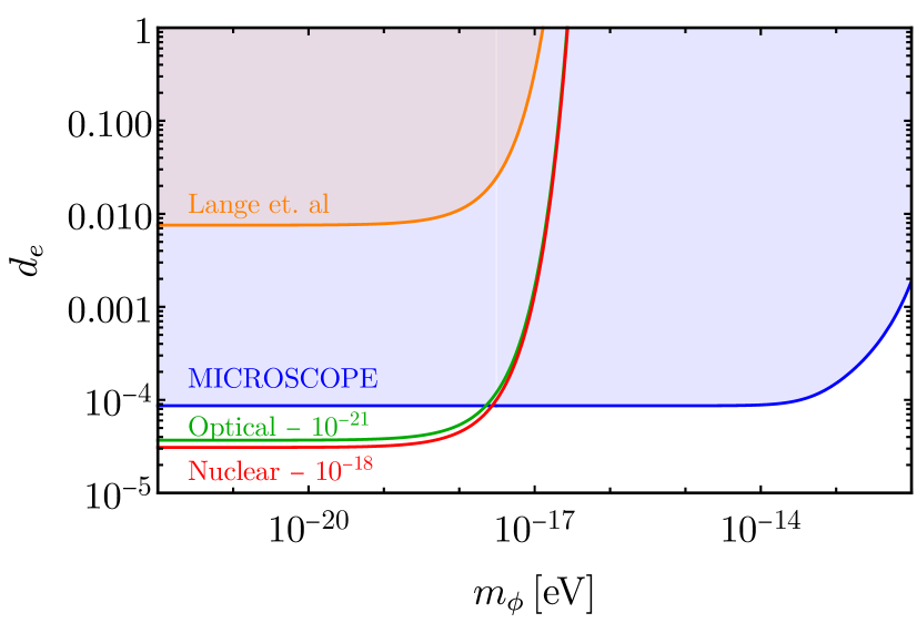
Figure 5: In the $d_{e}$ vs. $m_{\phi}$ plane, we show how the projected limits from future earth based two-clock experiments compare against the current bounds from direct fifth force searches. The orange region represents the current bounds from atomic clock experiments Lange:2020cul . The blue region shows the parameter space excluded by the MICROSCOPE experiment Touboul:2017grn ; Berge2017_MICROSCOPE . The green line depicts the projected limit from a future Earth based experiment involving two optical clocks with $\Delta K_{\alpha}=7$ and ${\Delta\tilde{f}}/{\tilde{f}}=10^{-21}$. The red line shows the projected sensitivity of an Earth based two-clock experiment involving a nuclear clock with $\Delta K_{\alpha}=10^{4}$ and ${\Delta\tilde{f}}/{\tilde{f}}=10^{-18}$.

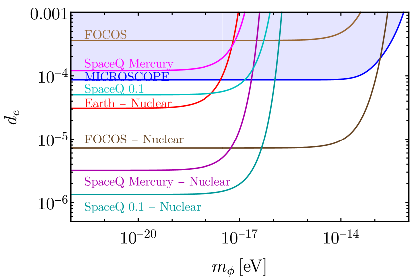
Figure 6: In the $d_{e}$ vs. $m_{\phi}$ plane we show how the projected limits from future experiments compare against the current bound from direct fifth force searches. The blue region shows the parameter space excluded by the MICROSCOPE experiment Touboul:2017grn ; Berge2017_MICROSCOPE . The red line shows the sensitivity of an Earth based two-clock experiment involving a nuclear clock with $\Delta K_{\alpha}=10^{4}$ and $\Delta\tilde{f}/\tilde{f}=10^{-18}$. The brown and dark brown lines show the potential reach of the FOCOS experiment Derevianko:2021kye , assuming that the satellite is equipped with an optical clock with $K_{\alpha}=-6$ or a nuclear clock with $K_{\alpha}=10^{4}$ respectively and measures the redshift with the accuracy of $\beta=10^{-9}$. The magenta and cyan lines depict the sensitivity of the SpaceQ mission Tsai:2021lly while traveling towards the $r=0.39$ AU and $r=0.1$ AU orbits respectively, assuming that the satellite is equipped with two optical clocks with $\Delta K_{\alpha}=7$ and $\Delta\tilde{f}/\tilde{f}=10^{-18}$. The dark magenta and dark cyan lines depict the ultimate sensitivities of the SpaceQ experiment while traveling towards the $r=0.39$ AU and $r=0.1$ AU orbits respectively, when the satellite is equipped with a nuclear-optical clock system with $\Delta K_{\alpha}=10^{4}$ and $\Delta\tilde{f}/\tilde{f}=10^{-18}$.

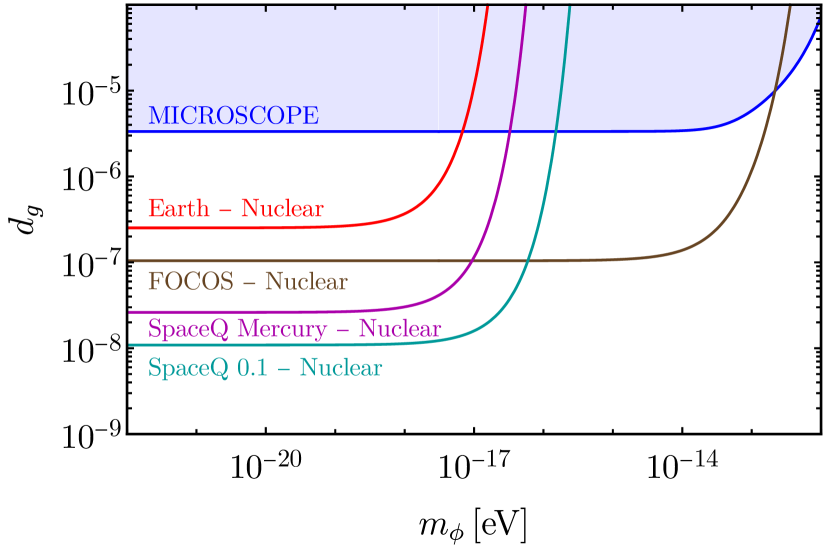
Figure 7: In the $d_{g}$ vs. $m_{\phi}$ plane we show how the projected limits from future clock based experiments compare against the current bounds on fifth forces. The blue region shows the parameter space excluded by the MICROSCOPE experiment Berge2017_MICROSCOPE ; Touboul:2017grn . The red line depicts the projected sensitivity of an Earth based two-clock experiment involving a nuclear clock, the dark brown line shows the projected reach of the space based FOCOS experiment equipped with a nuclear clock, while the dark magenta and dark cyan lines project the sensitivities of the SpaceQ experiment assuming that the satellite reaches $r=0.39$AU and $r=0.1$AU respectively and is equipped with nuclear clocks. We take $\Delta K_{q}=10^{5}$ and $\Delta\tilde{f}/\tilde{f}=10^{-18}$ for all clock pairs except for the FOCOS experiment where we assume $\beta=10^{-9}$.

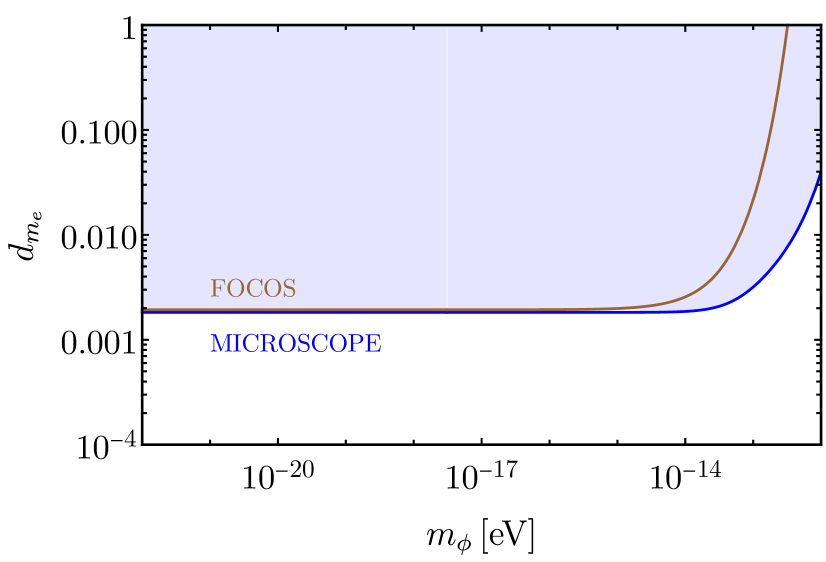
Figure 8: In the $d_{m_{e}}$ vs. $m_{\phi}$ plane we show how the projected limit from the future space based FOCOS experiment compares against the current bound. The blue region shows the parameter space excluded by the MICROSCOPE experiment Berge2017_MICROSCOPE ; Touboul:2017grn while the brown line shows the reach of the FOCOS experiment Derevianko:2021kye assuming that the satellite is equipped with an optical clock with $K_{\alpha}=-6$ and the redshift is measured with the accuracy of $\beta=10^{-9}$.

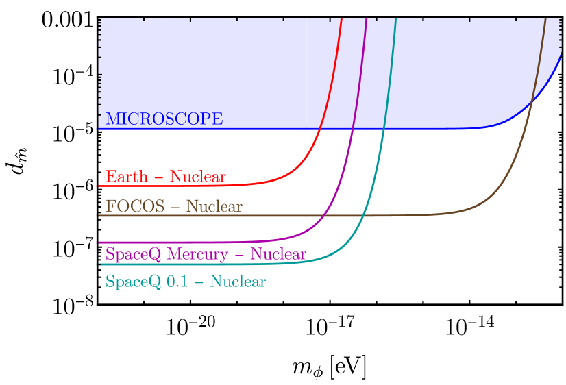
Figure 9: In the $d_{\hat{m}}$ vs. $m_{\phi}$ plane, we show how the projected limits from future clock based experiments compare against the current bounds from direct fifth force searches. The blue region shows the parameter space excluded by the MICROSCOPE experiment Berge2017_MICROSCOPE ; Touboul:2017grn . The red line gives the sensitivity of an Earth based two-clock experiment involving a nuclear clock, the dark brown line depicts the reach of the space based FOCOS experiment equipped with a nuclear clock while the dark magenta and dark cyan lines project the sensitivities of the space based SpaceQ experiment assuming that the satellite reaches $r=0.39$AU and $r=0.1$AU respectively and is equipped with a nuclear clock. We assume $\Delta K_{q}=10^{5}$ and $\Delta\tilde{f}/\tilde{f}=10^{-18}$ for all clock pairs except for the FOCOS experiment where we assume $\beta=10^{-9}$.

III.1 Two Different Clocks at the Same Location

In order to match the sensitivity of the direct fifth force searches by the MICROSCOPE experiment Berge2017_MICROSCOPE ; Touboul:2017grn , the uncertainty in the frequency of optical clocks located on earth needs to be of order ${\Delta\tilde{f}}/{\tilde{f}}\sim 10^{-21}$ for $\Delta K_{\alpha}=7$. This requires an improvement by about 3 orders of magnitude over the best precision available at this time, which is expected to occur within the next two decades Derevianko:2021kye .

However, improved precision is not the only option. Clocks based on nuclear transitions offer the exciting prospect of measuring the variation of fundamental constants with unprecedented sensitivity Peik:2020cwm . The nuclear clock based on the ²²⁹Th nucleus is expected to have sensitivity to the variation of the fine structure constant about 3 orders of magnitude better than the best optical clock, $K_{\alpha}\sim 10^{4}$, while the sensitivity to the masses of the quarks is expected to be even greater, $K_{q}\sim 10^{5}$ Flambaum:2008kr . Because of the large $K_{q}$, nuclear clocks of this type with an uncertainty of ${\Delta\tilde{f}}/{\tilde{f}}\sim 10^{-18}$ would be sufficient to improve on the current bounds set by the MICROSCOPE experiment. This is shown in Figs. 4, 8, 8 , and 8.

Another possibility is to conduct an experiment in space. By sending the two clocks closer to the sun we can take advantage of the larger gravitational potential to increase the sensitivity to $(\beta_{A}-\beta_{B})$. SpaceQ is a recent proposal based on this strategy Tsai:2021lly . The satellite would be equipped with a two-clock system, and the frequency ratio between the clocks as the satellite orbits the sun would be measured. The first stage of the experiment proposes to send a satellite to Mercury’s orbit, which is at $r=0.39$ AU. The second stage could reach down to $r=0.1$ AU. In both these stages the satellite’s orbit is designed to be circular, which means that during the main stage of the experiment EP violating effects would not be measurable. However, as pointed out in the proposal, data can also be taken as the satellite transits towards its final orbit, allowing us to measure EP violating effects. In reaching the $r=0.1$ AU orbit, the satellite would experience a change in the gravitational potential of the order of $\Delta U\sim 10^{-7}$, which is greater than the annual modulation of the gravitational potential on earth by a factor of nearly 300. In Fig. 8 we illustrate the sensitivity of this proposal to $d_{e}$ in four different scenarios. In the first case a satellite is sent out to Mercury’s orbit containing two optical clocks. In the second case, one of the optical clocks is replaced by a nuclear clock. In the third and fourth cases a satellite is sent to orbit the sun at $r=0.1$ AU with an optical-optical and a nuclear-optical clock system respectively. In all versions of the experiment we assume a fractional uncertainty of ${\Delta\tilde{f}}/{\tilde{f}}\sim 10^{-18}$. We see that the use of nuclear clocks leads to great improvements over the current sensitivity.

III.2 Identical Spatially Separated Clocks

The FOCOS experiment Derevianko:2021kye proposes to place a satellite carrying an optical clock in an elliptical orbit around the earth. The clock on the satellite will communicate with an identical clock on earth via optical links as the satellite approaches its apogee and perigee. Since the distance between the surface of the earth and the satellite will vary between 5000 km and 22500 km, the satellite will experience a large variation in the earth’s gravitational potential, allowing for an accurate determination of $\beta_{A}$. The optical clock offers more stability and precision than the microwave clocks that were used in earlier satellites. Instead of continuous monitoring of the frequency ratio, the experiment would monitor the phase difference between the clocks which can be translated into a frequency difference. This ultimately can be transformed into a limit on $\beta_{A}$ using Eq. (35). The experiment aims to measure $\beta_{A}$ with an accuracy of $10^{-9}$.

As explained in Sec. II.2, the bound on the anomalous redshift can be translated into bounds on the parameters $D_{x}$ and $d_{x}$ through Eq. (26). Since the proposal did not specify the clocks that would be used on the mission, we will consider two scenarios. In the first scenario, the satellite is equipped with an optical clock based on the electric octopole transition (E3) of ${}^{171}\text{Yb}^{+}$, which has the highest realized sensitivity to the variation of the fine structure constant, $K_{\alpha}=-6$ Flambaum:2008kr . In the second scenario, we consider a satellite with a nuclear clock that has a sensitivity of $K_{\alpha}\sim 10^{4}$. The expected experimental reach of these two versions of the FOCOS experiment for the couplings $d_{e}$, $d_{g}$, $d_{m_{e}}$ and $d_{\hat{m}}$ is presented in Figs. 8, 8, 8 and 9. Remarkably, we see from Fig. 8 that with even with existing clock technology the FOCOS experiment would be competitive with the currents bounds on $d_{m_{e}}$ from direct fifth force searches. However, to improve on the current limits on $d_{e}$, $d_{g}$ and $d_{\hat{m}}$ would require the use of nuclear clocks.

It follows from this discussion that, when it comes to fifth forces mediated by scalars that couple primarily to electrons, satellite-based clock experiments can already compete with direct fifth force searches. The reason why this particular coupling is where clocks first start to gain ground is because the frequencies associated with most atomic transitions are directly proportional to $m_{e}$, and so they are very sensitive to changes in the electron mass. In contrast, in direct fifth force searches, the electron only contributes a small amount to the mass of any given atom and so these experiments are inherently less sensitive to forces that act primarily on electrons.

IV Conclusions

In this article, we have explored how clock based experiments offer an alternative approach to probing EP violating fifth forces mediated by ultralight scalars. The same scalar field that mediates the fifth force will, in general, also give rise to position dependence in the fundamental parameters. Clocks on the earth as it orbits the sun or clocks on satellites orbiting the earth are sensitive to this effect, and therefore provide an excellent opportunity to test this class of models. The sensitivity of clock based experiments can be compared against the limits from direct fifth force searches, providing a benchmark to aim for when designing these experiments.

We have considered two classes of experiments utilizing clocks. The first class of experiments we studied were differential measurements where two different clock transitions were being compared at the same location. These experiments, performed on earth or in space, have the potential to probe beyond the current limits but require clocks more sensitive than currently available. The second class of experiments are anomalous redshift measurements where a clock in an elliptical orbit around the earth is compared to a clock on earth. Experiments along these lines utilizing current clock technology can place constraints on fifth forces that act primarily on electrons that are competitive with current constraints. Future nuclear clocks in elliptical orbits would offer a significant improvement in sensitivity to several different couplings.

The rapid experimental progress in clock technology has been quite remarkable. Their sensitivity has been consistently improving by an order of magnitude every few years for the past several decades. Our analysis shows that if this rate of improvement is maintained, clock experiments may soon offer the greatest sensitivity to EP violating fifth forces mediated by ultralight scalar fields.

Appendix A Effect of Uncertainty in the Earth’s Gravitational Potential on Anomalous Redshift Measurements

Fifth force searches based on anomalous redshift measurements require a knowledge of the general relativistic contribution to the redshift to the corresponding level of accuracy. Therefore uncertainties in our knowledge of the earth’s gravitational field can limit the precision of the determination of the anomalous redshift. In this respect anomalous redshift measurements differ from direct fifth force searches or differential redshift measurements, for which the effect of the uncertainties in the earth’s gravitational field is small because they compare the motion of two bodies of different compositions or two different clocks at the same physical location. In the neighborhood of the earth, the gravitational potential is determined from the precisely measured orbits of many different satellites under the assumption that they are acted on only by the gravitational force. However, as emphasized throughout this paper, models which give rise to position dependence of fundamental parameters also predict a fifth force. This fifth force will affect the orbit of satellites and will therefore affect the inferred value of the gravitational potential. In this appendix, we systematically take this effect into account and show that the corrections to our formulas are small.

Anomalous redshift experiments employ a clock placed on a satellite in orbit around the earth. The frequency of this clock is measured at different locations and compared against the frequency of an identical clock on earth. The anomalous redshift $\tilde{\beta}_{A}$ inferred from these experiments is related to the frequency change of the clock as,

$$\frac{\Delta f}{f}=(1+\tilde{\beta}_{A})\Delta\tilde{U}_{\rm infer}\;,$$ (36)

Here $\tilde{U}_{\rm infer}$ is the inferred value of the difference in the gravitational potential as opposed to its actual value $\Delta U_{\text{GR}}$. In the class of theories we are exploring, this observed change in frequency actually arises from two separate contributions, one from general relativity and the other from the location dependence of fundamental constants. Together, these read

$$\frac{\Delta f}{f}=\Delta U_{\text{GR}}+\beta_{A}\Delta U_{\text{GR}}\;,$$ (37)

where the first term is the difference predicted by general relativity while the second term is what was calculated in the text, see e.g. Eq. (24). To translate the experimental bound on $\tilde{\beta}_{A}$ to a constraint on $\beta_{A}$, we need to relate $\tilde{U}_{\rm infer}$ to $U_{\text{GR}}$.

The gravitational potential is inferred from the motion of satellites. The acceleration of a satellite in the earth’s gravitational field is given by,

$$a=\frac{GM}{r^{2}}\left(1+\alpha_{\text{\bf E}}\alpha_{\text{\bf S}}\right)=\frac{\Delta U_{\text{infer}}}{r},$$ (38)

where $\alpha_{\bf E}$ and $\alpha_{\bf S}$ represent the values of $\alpha_{\bf X}$ for the earth and satellite respectively, where $\alpha_{\bf X}$ is as defined in Eq. (5). For simplicity we have taken the mass of the ultralight scalar to be zero, since incorporating a non-zero mass for the modulus would require a detailed understanding of the orbits of the satellites employed.

Using the relationship $\Delta U_{\text{GR}}=GM/r$ and Eqs. (36), (37) and (38), we find that

$$\tilde{\beta}_{A}\approx\beta_{A}-\alpha_{\bf E}\alpha_{\bf S}.$$ (39)

From Eq. (26) we have

$$\frac{\beta_{A}}{\alpha_{\bf E}}=\left[(K^{A}_{\alpha}+2)d_{e}-K^{A}_{\mu}(d_{m_{e}}-d_{g})+K^{A}_{q}(d_{\hat{m}}-d_{g})+d_{m_{e}}\right]\;.$$ (40)

Then the inferred anomalous redshift $\tilde{\beta}_{A}$ is proportional to the difference

$$\tilde{\beta}_{A}\propto F(K_{X}^{A},d_{x})-\alpha_{\bf S}\;,$$ (41)

where $F(K_{X}^{A},d_{x})$ is the term on the right hand side of Eq. (40). From the expression for $\alpha_{\bf S}$ in Eqs. (5) and (7), we see that this difference is the sum of a term proportional to $d_{e}$, a term proportional to $(d_{m_{e}}-d_{g})$ and a term proportional to $(d_{\hat{m}}-d_{g})$. As we now explain, this is exactly as expected. Recall that experiments cannot distinguish an EP preserving dilaton from general relativity in the non-relativistic limit. Setting the couplings to their values in the dilaton limit, $d_{g}=d_{m_{e}}=d_{\hat{m}}$ and $d_{e}=0$, we find that $\tilde{\beta}_{A}=0$ as expected. This constitutes a powerful cross check of our results.

From Eq. (7) we see that the parameters $Q_{\hat{m}}$, $Q_{e}$ and $Q_{m_{e}}$ are all much less than one. This allows us to approximate

$$\frac{\tilde{\beta}_{A}}{\alpha_{\bf E}}\approx\left[(K^{A}_{\alpha}+2)d_{e}+(1-K^{A}_{\mu})(d_{m_{e}}-d_{g})+K^{A}_{q}(d_{\hat{m}}-d_{g})\right]\;.$$ (42)

Comparing the right hand sides of Eqs. (42) and (40), we see that the difference between the two is just $d_{g}$. While the actual anomalous redshift scales with $d_{g}$ as $\beta_{A}/\alpha_{\bf E}\sim(K^{A}_{\mu}-K^{A}_{q})d_{g}$, the inferred anomalous redshift scales as $\tilde{\beta}_{A}/\alpha_{\bf E}\sim(K^{A}_{\mu}-K^{A}_{q}-1)d_{g}$. Thus the errors arising from neglecting the effect of the fifth force on the motion of the satellite are small provided that either $d_{g}$ is negligible or $|K_{\mu}^{A}+K^{A}_{q}|\gg 1$. For the clocks used in the experiments we have considered, the second condition is satisfied.

References

- (1) E. Fischbach and C. Talmadge, The search for nonNewtonian gravity, .
- (2) E. G. Adelberger, B. R. Heckel, and A. E. Nelson, Tests of the gravitational inverse square law, Ann. Rev. Nucl. Part. Sci. 53 (2003) 77–121, [hep-ph/0307284].
- (3) T. Damour and A. M. Polyakov, The String dilaton and a least coupling principle, Nucl. Phys. B 423 (1994) 532–558, [hep-th/9401069].
- (4) T. Damour and A. M. Polyakov, String theory and gravity, Gen. Rel. Grav. 26 (1994) 1171–1176, [gr-qc/9411069].
- (5) A. Hook, Solving the Hierarchy Problem Discretely, Phys. Rev. Lett. 120 (2018), no. 26 261802, [arXiv:1802.10093].
- (6) D. Brzeminski, Z. Chacko, A. Dev, and A. Hook, Time-varying fine structure constant from naturally ultralight dark matter, Phys. Rev. D 104 (2021), no. 7 075019, [arXiv:2012.02787].
- (7) M. S. Turner, Coherent Scalar Field Oscillations in an Expanding Universe, Phys. Rev. D 28 (1983) 1243.
- (8) W. H. Press, B. S. Ryden, and D. N. Spergel, Single Mechanism for Generating Large Scale Structure and Providing Dark Missing Matter, Phys. Rev. Lett. 64 (1990) 1084.
- (9) S.-J. Sin, Late time cosmological phase transition and galactic halo as Bose liquid, Phys. Rev. D 50 (1994) 3650–3654, [hep-ph/9205208].
- (10) A. Khmelnitsky and V. Rubakov, Pulsar timing signal from ultralight scalar dark matter, JCAP 02 (2014) 019, [arXiv:1309.5888].
- (11) Y. Stadnik and V. Flambaum, Searching for dark matter and variation of fundamental constants with laser and maser interferometry, Phys. Rev. Lett. 114 (2015) 161301, [arXiv:1412.7801].
- (12) A. Arvanitaki, S. Dimopoulos, and K. Van Tilburg, Sound of Dark Matter: Searching for Light Scalars with Resonant-Mass Detectors, Phys. Rev. Lett. 116 (2016), no. 3 031102, [arXiv:1508.01798].
- (13) P. W. Graham, I. G. Irastorza, S. K. Lamoreaux, A. Lindner, and K. A. van Bibber, Experimental Searches for the Axion and Axion-Like Particles, Ann. Rev. Nucl. Part. Sci. 65 (2015) 485–514, [arXiv:1602.00039].
- (14) P. W. Graham, D. E. Kaplan, J. Mardon, S. Rajendran, and W. A. Terrano, Dark Matter Direct Detection with Accelerometers, Phys. Rev. D 93 (2016), no. 7 075029, [arXiv:1512.06165].
- (15) Y. Stadnik and V. Flambaum, Enhanced effects of variation of the fundamental constants in laser interferometers and application to dark matter detection, Phys. Rev. A 93 (2016), no. 6 063630, [arXiv:1511.00447].
- (16) A. Berlin, Neutrino Oscillations as a Probe of Light Scalar Dark Matter, Phys. Rev. Lett. 117 (2016), no. 23 231801, [arXiv:1608.01307].
- (17) A. A. Geraci and A. Derevianko, Sensitivity of atom interferometry to ultralight scalar field dark matter, Phys. Rev. Lett. 117 (2016), no. 26 261301, [arXiv:1605.04048].
- (18) G. Krnjaic, P. A. Machado, and L. Necib, Distorted neutrino oscillations from time varying cosmic fields, Phys. Rev. D 97 (2018), no. 7 075017, [arXiv:1705.06740].
- (19) A. Arvanitaki, S. Dimopoulos, and K. Van Tilburg, Resonant absorption of bosonic dark matter in molecules, Phys. Rev. X 8 (2018), no. 4 041001, [arXiv:1709.05354].
- (20) W. DeRocco and A. Hook, Axion interferometry, Phys. Rev. D 98 (2018), no. 3 035021, [arXiv:1802.07273].
- (21) A. A. Geraci, C. Bradley, D. Gao, J. Weinstein, and A. Derevianko, Searching for Ultralight Dark Matter with Optical Cavities, Phys. Rev. Lett. 123 (2019), no. 3 031304, [arXiv:1808.00540].
- (22) I. G. Irastorza and J. Redondo, New experimental approaches in the search for axion-like particles, Prog. Part. Nucl. Phys. 102 (2018) 89–159, [arXiv:1801.08127].
- (23) D. Carney, A. Hook, Z. Liu, J. M. Taylor, and Y. Zhao, Ultralight Dark Matter Detection with Mechanical Quantum Sensors, arXiv:1908.04797.
- (24) H.-K. Guo, K. Riles, F.-W. Yang, and Y. Zhao, Searching for Dark Photon Dark Matter in LIGO O1 Data, Commun. Phys. 2 (2019) 155, [arXiv:1905.04316].
- (25) H. Grote and Y. Stadnik, Novel signatures of dark matter in laser-interferometric gravitational-wave detectors, Phys. Rev. Res. 1 (2019), no. 3 033187, [arXiv:1906.06193].
- (26) A. Dev, P. A. Machado, and P. Martínez-Miravé, Signatures of Ultralight Dark Matter in Neutrino Oscillation Experiments, arXiv:2007.03590.
- (27) V. B. Braginskii and V. I. Panov, Verification of equivalence of inertial and gravitational masses, Zh. Eksp. Teor. Fiz. 61 (1971) 873–879.
- (28) S. Schlamminger, K. Y. Choi, T. A. Wagner, J. H. Gundlach, and E. G. Adelberger, Test of the equivalence principle using a rotating torsion balance, Phys. Rev. Lett. 100 (2008) 041101, [arXiv:0712.0607].
- (29) E. G. Adelberger, J. H. Gundlach, B. R. Heckel, S. Hoedl, and S. Schlamminger, Torsion balance experiments: A low-energy frontier of particle physics, Prog. Part. Nucl. Phys. 62 (2009) 102–134.
- (30) T. A. Wagner, S. Schlamminger, J. H. Gundlach, and E. G. Adelberger, Torsion-balance tests of the weak equivalence principle, Class. Quant. Grav. 29 (2012) 184002, [arXiv:1207.2442].
- (31) P. Touboul et al., MICROSCOPE Mission: First Results of a Space Test of the Equivalence Principle, Phys. Rev. Lett. 119 (2017), no. 23 231101, [arXiv:1712.01176].
- (32) J. O. Dickey et al., Lunar Laser Ranging: A Continuing Legacy of the Apollo Program, Science 265 (1994) 482–490.
- (33) J. G. Williams, S. G. Turyshev, and D. H. Boggs, Progress in lunar laser ranging tests of relativistic gravity, Phys. Rev. Lett. 93 (2004) 261101, [gr-qc/0411113].
- (34) S. M. Ransom et al., A millisecond pulsar in a stellar triple system, Nature 505 (2014) 520, [arXiv:1401.0535].
- (35) A. M. Archibald, N. V. Gusinskaia, J. W. T. Hessels, A. T. Deller, D. L. Kaplan, D. R. Lorimer, R. S. Lynch, S. M. Ransom, and I. H. Stairs, Universality of free fall from the orbital motion of a pulsar in a stellar triple system, Nature 559 (2018), no. 7712 73–76, [arXiv:1807.02059].
- (36) S. Fray, C. Alvarez Diez, T. W. Hansch, and M. Weitz, Atomic interferometer with amplitude gratings of light and its applications to atom based tests of the equivalence principle, Phys. Rev. Lett. 93 (2004) 240404, [physics/0411052].
- (37) L. Zhou et al., Test of Equivalence Principle at Level by a Dual-species Double-diffraction Raman Atom Interferometer, Phys. Rev. Lett. 115 (2015), no. 1 013004, [arXiv:1503.00401].
- (38) L. Zhou et al., Joint mass-and-energy test of the equivalence principle at the 10-10 level using atoms with specified mass and internal energy, Phys. Rev. A 104 (2021), no. 2 022822, [arXiv:1904.07096].
- (39) D. Schlippert, J. Hartwig, H. Albers, L. L. Richardson, C. Schubert, A. Roura, W. P. Schleich, W. Ertmer, and E. M. Rasel, Quantum Test of the Universality of Free Fall, Phys. Rev. Lett. 112 (2014) 203002, [arXiv:1406.4979].
- (40) M. G. Tarallo, T. Mazzoni, N. Poli, D. V. Sutyrin, X. Zhang, and G. M. Tino, Test of Einstein Equivalence Principle for 0-spin and half-integer-spin atoms: Search for spin-gravity coupling effects, Phys. Rev. Lett. 113 (2014) 023005, [arXiv:1403.1161].
- (41) M. S. Safronova, D. Budker, D. DeMille, D. F. J. Kimball, A. Derevianko, and C. W. Clark, Search for New Physics with Atoms and Molecules, Rev. Mod. Phys. 90 (2018), no. 2 025008, [arXiv:1710.01833].
- (42) MAGIS-100 Collaboration, M. Abe et al., Matter-wave Atomic Gradiometer Interferometric Sensor (MAGIS-100), Quantum Sci. Technol. 6 (2021), no. 4 044003, [arXiv:2104.02835].
- (43) G. M. Tino, L. Cacciapuoti, S. Capozziello, G. Lambiase, and F. Sorrentino, Precision Gravity Tests and the Einstein Equivalence Principle, Prog. Part. Nucl. Phys. 112 (2020) 103772, [arXiv:2002.02907].
- (44) A. D. Ludlow, M. M. Boyd, J. Ye, E. Peik, and P. O. Schmidt, Optical atomic clocks, Rev. Mod. Phys. 87 (Jun, 2015) 637–701, [arXiv:1407.3493].
- (45) W. F. McGrew et al., Atomic clock performance enabling geodesy below the centimetre level, Nature 564 (2018), no. 7734 87–90, [arXiv:1807.11282].
- (46) G. E. Marti, R. B. Hutson, A. Goban, S. L. Campbell, N. Poli, and J. Ye, Imaging optical frequencies with precision and resolution, Phys. Rev. Lett. 120 (Mar, 2018) 103201, [arXiv:1711.08540].
- (47) T. Bothwell, D. Kedar, E. Oelker, J. M. Robinson, S. L. Bromley, W. L. Tew, J. Ye, and C. J. Kennedy, JILA SrI optical lattice clock with uncertainty of , Metrologia 56 (oct, 2019) 065004, [arXiv:1906.06004].
- (48) V. V. Flambaum and E. V. Shuryak, How changing physical constants and violation of local position invariance may occur?, AIP Conf. Proc. 995 (2008), no. 1 1–11, [physics/0701220].
- (49) D. J. Shaw, Detecting seasonal changes in the fundamental constants, gr-qc/0702090.
- (50) J. D. Barrow and D. J. Shaw, Varying Alpha: New Constraints from Seasonal Variations, Phys. Rev. D 78 (2008) 067304, [arXiv:0806.4317].
- (51) T. Dent, Eotvos bounds on couplings of fundamental parameters to gravity, Phys. Rev. Lett. 101 (2008) 041102, [arXiv:0805.0318].
- (52) J.-P. Uzan, Varying Constants, Gravitation and Cosmology, Living Rev. Rel. 14 (2011) 2, [arXiv:1009.5514].
- (53) J. Khoury and A. Weltman, Chameleon fields: Awaiting surprises for tests of gravity in space, Phys. Rev. Lett. 93 (2004) 171104, [astro-ph/0309300].
- (54) J. Khoury and A. Weltman, Chameleon cosmology, Phys. Rev. D 69 (2004) 044026, [astro-ph/0309411].
- (55) B. Feldman and A. E. Nelson, New regions for a chameleon to hide, JHEP 08 (2006) 002, [hep-ph/0603057].
- (56) D. F. Mota and D. J. Shaw, Strongly coupled chameleon fields: New horizons in scalar field theory, Phys. Rev. Lett. 97 (2006) 151102, [hep-ph/0606204].
- (57) P. Brax, C. Burrage, and A.-C. Davis, Laboratory constraints, Int. J. Mod. Phys. D 27 (2018), no. 15 1848009.
- (58) J. Sakstein, Astrophysical tests of screened modified gravity, Int. J. Mod. Phys. D 27 (2018), no. 15 1848008, [arXiv:2002.04194].
- (59) N. Blinov, S. A. Ellis, and A. Hook, Consequences of Fine-Tuning for Fifth Force Searches, JHEP 11 (2018) 029, [arXiv:1807.11508].
- (60) R. F. C. Vessot and M. W. Levine, A test of the equivalence principle using a space-borne clock, General Relativity and Gravitation 10 (1979) 181204.
- (61) P. Delva et al., Gravitational Redshift Test Using Eccentric Galileo Satellites, Phys. Rev. Lett. 121 (2018), no. 23 231101, [arXiv:1812.03711].
- (62) A. Derevianko, K. Gibble, L. Hollberg, N. R. Newbury, C. Oates, M. S. Safronova, L. C. Sinclair, and N. Yu, Fundamental Physics with a State-of-the-Art Optical Clock in Space, arXiv:2112.10817.
- (63) Y.-D. Tsai, J. Eby, and M. S. Safronova, SpaceQ - Direct Detection of Ultralight Dark Matter with Space Quantum Sensors, arXiv:2112.07674.
- (64) V. Schkolnik et al., Optical Atomic Clock aboard an Earth-orbiting Space Station (OACESS): Enhancing searches for physics beyond the standard model in space, arXiv:2204.09611.
- (65) T. Damour and J. F. Donoghue, Equivalence Principle Violations and Couplings of a Light Dilaton, Phys. Rev. D 82 (2010) 084033, [arXiv:1007.2792].
- (66) T. Damour and J. F. Donoghue, Phenomenology of the Equivalence Principle with Light Scalars, Class. Quant. Grav. 27 (2010) 202001, [arXiv:1007.2790].
- (67) J. Bergé, P. Brax, G. Métris, M. Pernot-Borràs, P. Touboul, and J.-P. Uzan, MICROSCOPE Mission: First Constraints on the Violation of the Weak Equivalence Principle by a Light Scalar Dilaton, Phys. Rev. Lett. 120 (2018), no. 14 141101, [arXiv:1712.00483].
- (68) N. Leefer, C. T. M. Weber, A. Cingöz, J. R. Torgerson, and D. Budker, New limits on variation of the fine-structure constant using atomic dysprosium, Phys. Rev. Lett. 111 (Aug, 2013) 060801, [arXiv:1304.6940].
- (69) N. Leefer, A. Gerhardus, D. Budker, V. V. Flambaum, and Y. V. Stadnik, Search for the effect of massive bodies on atomic spectra and constraints on Yukawa-type interactions of scalar particles, Phys. Rev. Lett. 117 (2016), no. 27 271601, [arXiv:1607.04956].
- (70) R. Lange, N. Huntemann, J. M. Rahm, C. Sanner, H. Shao, B. Lipphardt, C. Tamm, S. Weyers, and E. Peik, Improved limits for violations of local position invariance from atomic clock comparisons, Phys. Rev. Lett. 126 (2021), no. 1 011102, [arXiv:2010.06620].
- (71) E. Peik, T. Schumm, M. S. Safronova, A. Pálffy, J. Weitenberg, and P. G. Thirolf, Nuclear clocks for testing fundamental physics, Quantum Sci. Technol. 6 (2021), no. 3 034002, [arXiv:2012.09304].
- (72) V. V. Flambaum and V. A. Dzuba, Search for variation of the fundamental constants in atomic, molecular and nuclear spectra, Can. J. Phys. 87 (2009) 25–33, [arXiv:0805.0462].